Scientific, Technical and Economic Committee for Fisheries ...18-01... · This publication is a Science for Policy report by the Joint Research Centre (JRC), the European Commission’s

Scientific, Technical and Economic

Committee for Fisheries (STECF)

-

Monitoring the performance of the

Common Fisheries Policy

(STECF-Adhoc-18-01)

Edited by Ernesto Jardim, Paris Vasilakopoulos, Alessandro Mannini, Iago

Mosqueira and John Casey

EUR 29223 EN

This publication is a Science for Policy report by the Joint Research Centre (JRC), the European

Commission’s science and knowledge service. It aims to provide evidence-based scientific support to

the European policy-making process. The scientific output expressed does not imply a policy position of

the European Commission. Neither the European Commission nor any person acting on behalf of the

Commission is responsible for the use which might be made of this publication.

Contact information

Name: STECF secretariat

Address: Unit D.02 Water and Marine Resources, Via Enrico Fermi 2749, 21027 Ispra VA, Italy

E-mail: [email protected]

Tel.: +39 0332 789343

JRC Science Hub

https://ec.europa.eu/jrc

JRC111761

EUR 29223 EN

PDF ISBN 978-92-79-85802-4 ISSN 1831-9424 doi:10.2760/329345

STECF ISSN 2467-0715

Luxembourg: Publications Office of the European Union, 2018

© European Union, 2018

Reuse is authorised provided the source is acknowledged. The reuse policy of European Commission

documents is regulated by Decision 2011/833/EU (OJ L 330, 14.12.2011, p. 39).

For any use or reproduction of photos or other material that is not under the EU copyright, permission

must be sought directly from the copyright holders.

How to cite: Scientific, Technical and Economic Committee for Fisheries (STECF) – Monitoring the

performance of the Common Fisheries Policy (STECF-Adhoc-18-01). Publications Office of the European

Union, Luxembourg, 2018, ISBN 978-92-79-85802-4, doi:10.2760/329345, JRC111761

All images © European Union 2018

Abstract

Commission Decision of 25 February 2016 setting up a Scientific, Technical and Economic Committee

for Fisheries, C(2016) 1084, OJ C 74, 26.2.2016, p. 4–10. The Commission may consult the group on

any matter relating to marine and fisheries biology, fishing gear technology, fisheries economics,

fisheries governance, ecosystem effects of fisheries, aquaculture or similar disciplines. This report deals

with monitoring the performance of the Common Fisheries Policy.

https://ec.europa.eu/jrc

3 3

Authors:

STECF advice:

Ulrich, C.., Abella, J. A., Andersen, J., Arrizabalaga, H., Bailey, N., Bertignac, M., Borges, L., Cardinale, M., Catchpole, T., Curtis, H., Daskalov, G., Döring, R., Gascuel, D., Knittweis, L.,

Malvarosa, L., Martin, P., Motova, A., Murua, H., Nord, J., Prellezo, R., Raid, T., Sabatella, E., Sala, A., Scarcella, G., Soldo, A., Somarakis, S., Stransky, C., van Hoof, L., Vanhee, W., Vrgoc,

Nedo.

Ad hoc Expert group report:

E. Jardim, P. Vasilakopoulos, A. Mannini, I. Mosqueira, J. Casey

4 4

TABLE OF CONTENTS

SCIENTIFIC, TECHNICAL AND ECONOMIC COMMITTEE FOR FISHERIES (STECF) -

Monitoring the performance of the Common Fisheries Policy (STECF-Adhoc-18-01) .......................................................................................................... 6

Background provided by the Commission ................................................................. 6

Request to the STECF ........................................................................................................ 6

STECF observations ............................................................................................................ 6

General principles for future analysis ........................................................................ 11

STECF conclusions ............................................................................................................. 12

Contact details of STECF members ............................................................................ 12

Expert Group Report ........................................................................................................ 17

1 Introduction ........................................................................................................... 18

1.1 Terms of Reference to the ad hoc Expert group ..................................... 18

2 Data and methods ............................................................................................... 19

2.1 Data sources .......................................................................................................... 19

2.1.1 Stock assessment information ....................................................................... 19

2.1.2 Management units information ...................................................................... 19

2.2 Methods ................................................................................................................... 19

2.3 Points to note ........................................................................................................ 19

2.4 Differences from the 2017 CFP monitoring report (STECF 17-04) .. 20

2.4.1 Northeast Atlantic ................................................................................................ 20

2.4.2 Mediterranean and Black Sea ......................................................................... 20

3 Northeast Atlantic and adjacent Seas (FAO region 27) ....................... 21

3.1 Number of stock assessments to compute CFP performance indicators .................................................................................................................................... 21

3.2 Indicators of management performance .................................................... 28

3.2.1 Number of stocks by year where fishing mortality exceeded FMSY .. 28

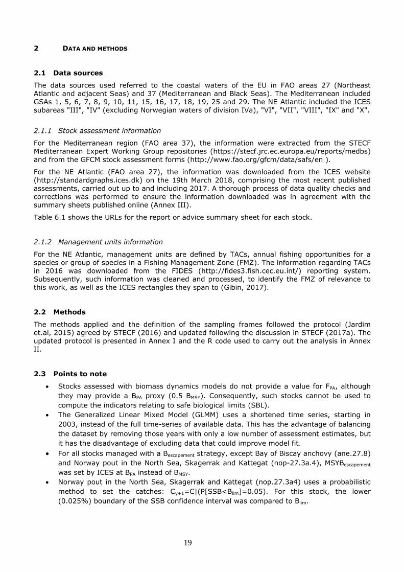
3.2.2 Number of stocks by year for which fishing mortality was equal to, or less than FMSY ................................................................................................................. 29

3.2.3 Number of stocks outside safe biological limits ....................................... 30

3.2.4 Number of stocks inside safe biological limits ......................................... 31

3.2.5 Trend in F/FMSY ...................................................................................................... 32

3.2.6 Trend in SSB (relative to 2003) ..................................................................... 34

3.3 Experimental indicators .................................................................................... 36

5 5

3.3.1 Number of stocks with F above Fmsy or SSB below MSYBtrigger ... 37

3.3.2 Number of stocks with F below or equal to Fmsy and SSB above or equal to MSYBtrigger ...................................................................................................... 38

3.3.3 Trend in F/FMSY for stocks outside the EU coastal waters .................... 39

3.3.4 Trend in SSB/Bpa .................................................................................................. 40

3.3.5 Trend in recruitment (relative to 2003) ..................................................... 41

3.3.6 Trend in SSB or biomass index for stocks of data category 1-3 (relative to 2003) ........................................................................................................................ 42

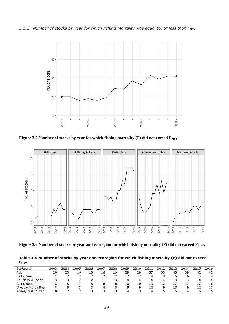
3.3.7 Trend in SSB or biomass index for stocks of data category 3 (relative to 2003) ........................................................................................................................ 43

3.4 Indicators of advice coverage ......................................................................... 44

4 Mediterranean and Black Seas (FAO region 37) ..................................... 45

4.1 Indicators of management performance .................................................... 48

4.1.1 Trend in F/FMSY ................................................................................................... 48

4.1.2 Trend in SSB (relative to 2003) ..................................................................... 49

4.2 Indicators of advice coverage ......................................................................... 50

5 Status across all stocks in 2016 .................................................................... 51

6 Reports by stock .................................................................................................. 55

7 References .............................................................................................................. 58

8 Contact details of ad hoc expert group participants .............................. 59

9 List of Annexes ..................................................................................................... 61

Annex I - Protocol .............................................................................................................. 62

Annex II - Code .................................................................................................................. 63

Annex III – Quality control of ICES dataset ........................................................... 64

6 6

SCIENTIFIC, TECHNICAL AND ECONOMIC COMMITTEE FOR FISHERIES (STECF) - Monitoring the performance of the Common Fisheries Policy (STECF-Adhoc-18-01)

Background provided by the Commission

Article 50 of the Common Fisheries Policy (CFP; Regulation (EU) No 1380/2013 of the European Parliament and of the Council of 11 December 2013) stipulates: “The Commission shall report

annually to the European Parliament and to the Council on the progress on achieving maximum sustainable yield and on the situation of fish stocks, as early as possible following the adoption of

the yearly Council Regulation fixing the fishing opportunities available in Union waters and, in

certain non-Union waters, to Union vessels.”

Request to the STECF

The STECF is requested to report on progress in achieving MSY objectives in line with the

Common Fisheries Policy.

STECF observations

STECF notes that to address the above Terms of Reference a JRC Expert Group (EG) was convened to compile available assessment outputs and conduct the extensive analysis. The EG

output was presented in a comprehensive report accompanied by several detailed annexes

providing: 1) CFP monitoring protocols as agreed by STECF (STECF, 2017); 2a) R code for computing NE Atlantic indicators; 2b) R code for computing Mediterranean indicators and 3) ICES

data quality issues corrected prior to the analysis. The report and Annexes are available at https://stecf.jrc.ec.europa.eu/plen18_01

STECF notes that the report is clear and well laid out, transparently describing the analysis undertaken, cataloguing changes made in approach since the previous report (2017) and

including URL links to the various reports and stock advice sheets underpinning the analysis. STECF commends the effort employed in updating nomenclature following various changes to the

ICES database and the careful attention paid to ensuring the correct figures were used.

The most significant changes in the 2018 approach were:

i) A revision of the Mediterranean sampling frame used for the analysis

ii) Where data were unavailable for the most recent year, the data from the previous year was rolled forward

iii) MSYBtrigger was used as a proxy for lower bound of BMSY

Details of these changes and other points to note can be found in section 2 of the EG report.

The EG report then sets out results of the analysis for the ICES area of the NE Atlantic and

Mediterranean & Black Sea separately in Sections 3 and 4 (respectively). Based on these results STECF provides an overview of what is currently known regarding the achievement of the MSY

objectives, drawing together the results from the different sea areas to provide a comparative picture. The overview focuses on a limited number of ‘core’ indicators earlier agreed by STECF

(2017). The EG report contains results for a number of ‘experimental’ indicators which STECF notes are still at the development stage. It is expected that these will be further developed as

part of another STECF EWG (EWG 18-15) to be held later in 2018 (see conclusions). In this report, “ICES Area” refers to all stocks in the FAO Area 27 in the Northeast Atlantic assessed by

ICES, while the denomination “NE Atlantic stocks” refers more specifically to the stocks

distributed widely, including outside EU Waters

https://stecf.jrc.ec.europa.eu/plen18_01

7 7

Trends towards the MSY objectives in the ICES area and Mediterranean& Black Seas

The overview below describes the trends observed in the ICES area and the Mediterranean for the periods 2003 to 2016 and 2003 to 2015 respectively and applies to the stocks included in the

reference list of stocks for these areas. The stocks are primarily those with a full analytical assessment (ICES Category 1).

Stock status in the ICES area

The indicators provided by the JRC EG show that stocks status has significantly improved (Figure 1) but also that many stocks are still overexploited in the ICES area, and that the rate of progress

has slowed in the last few years. In the ICES area, among the 65 to 71 stocks which are fully

assessed, the proportion of overexploited stocks (i.e. F>FMSY, blue line) decreased from more than 70% to close to 40%, over the last ten years and seems to have stabilised in the last three

years. The proportion of stocks outside the safe biological limits (F>Fpa or B<Bpa, orange line), computed for the 46 stocks for which both reference points are available, follows the same

decreasing trend, from 65% in 2003 to around 30% in 2016.

Figure 1. Trends in stocks status, 2003-2016. Three indicators are presented: Blue line: the proportion of overexploited stocks (F>FMSY) within the sampling frame (65 to 71 stocks fully

assessed in the ICES area, depending on year); Orange line: the proportion of stocks outside safe

biological limits (F>Fpa or B< Bpa) (46 stocks); Red line: F>FMSY or SSB <MSYBtrigger

It is important to note, however, that some stocks now managed according to FMSY may still be

outside safe biological limits, or conversely some stocks inside safe biological limits may still be overfished.

The red line illustrates changes in the proportion of stocks where F>FMSY or SSB <MSYBtrigger. Here the improvement in status has been slower with the indicator remaining above 75% of stocks

until 2007 before declining. The decline then appears to have stopped in 2013 and began to slowly increase again to about 60% of stocks in 2016 where F>FMSY or SSB <MSYBtrigger.

STECF notes that the number or proportion of stocks above/below BMSY is still unknown, because

an estimate of BMSY is only provided by ICES for very few stocks.

STECF observes that the recent slope of the indicators suggests that progress until 2016 has been

too slow to allow all stocks to be maintained or restored to at least the precautionary Bpa, and managed according to FMSY by 2020.

8 8

Stock Status in the Mediterranean & Black Sea

In the Mediterranean & Black Sea, the variable number of stocks contributing information in the early part of the time series renders the calculation of a robust indicator difficult and potentially

misleading. STECF suggests the possibility of investigating this in the future for a shorter time period (e.g. from 2008 to 2015 when the stock numbers appear to be more stable). For the

present STECF has utilised the summary Table 5.1 in the EG report to compute the F status for 2015 (last year in Mediterranean stock assessments). Out of 47 stocks, only around 13% (6

stocks) are not overfished, the majority are overfished.

Trends in the fishing pressure (Ratio of F/FMSY)

As agreed by STECF (2017) the Expert Group computed the trends in fishing pressure using a robust statistical model (Generalised Linear Mixed Effects Model, GLMM) accounting for the

variability of trends across stocks and including the computation of a confidence interval around the median. A large confidence interval means that different stocks have different trends.

Because this is a model-based indicator, and because the number of stocks is slightly different from last year, small differences in the resulting outcomes compared to last year’s report should

not be over interpreted.

This indicator can be used for regional comparison between the ICES area and Mediterranean &

Black Seas. In the ICES area, the model-based indicator of the fishing pressure (F/FMSY) shows an

overall downward trend over the period 2003-2015 (Figure 2). In the early 2000s, the median fishing mortality was more than 1.5 times larger than FMSY, but this has reduced and has now

stabilised around 1.0. Reaching FMSY for most stocks in the analysis would require the upper bound of the confidence interval in figure 3.1 in the EWG report to be around 1. STECF also notes

that this indicator of fishing pressure has not decreased since 2011.

The same model-based indicator was computed by the EG for an additional set of 9 stocks located

in the NE Atlantic, but outside EU waters. This indicator seems to confirm the positive overall trend observed in EU waters, with the median value of the F/FMSY indicator closely tracking that

produced for EU waters. STECF notes that the indicator for NE Atlantic stocks outside EU waters is

based on comparatively few stocks and thus should be considered with care.

Figure 2. Trends in the fishing pressure. Three model based indicators F/FMSY are presented (all

referring to the median value of the model): one for 48 EU stocks with appropriate information in the ICES area (red line); one for an additional set of 9 stocks also located in the NE Atlantic but

9 9

outside EU waters (green line), and one for the 47 assessed stocks from the Mediterranean and

Black Sea region (black line).

In contrast, the indicator computed for stocks from the Mediterranean Sea and Black Sea has remained at a very high level during the whole 2003-2015 period, with no decreasing trend. The

value of F/FMSY varies around 2.3 indicating that the stocks are being exploited on average at rates well above the FMSY CFP objective.

Trends in Biomass

The model-based indicator of the trend in biomass shows improvement in the ICES area, but not

in the Mediterranean and Black Sea (Figure 3). In the ICES area the biomass has been generally increasing since 2006, and was in 2016 on average around 39% higher than in 2003. This

represents a slight change from the reporting in 2016 reflecting the fact that the modelled trend incorporates new information. In the Mediterranean & Black Sea the uncertainty associated with

this indicator (see Figure 4.4 in the EWG report) makes it difficult to conclude anything about trend and the situation is essentially unchanged since the start of the series in 2003.

An improving trend is also observed for data poor stocks (Figure 3.23 in the EWG report), according to the indicator computed by the EG for 61 ICES Category 3 stocks. However, in view

of the fact that this indicator is still regarded as experimental, care in interpretation is required.

Figure 3. Trends in the indicators of stock biomass (median values of the model-based estimates

relative to 2003). Two indicators are presented: one for the ICES area (54 stocks considered, blue line); one for the Mediterranean region (47 stocks, black line). The EG noticed that a large

uncertainty is associated to these estimates, coming from the fact that the biomass estimates are quite variable from one year to the next.

Trends per Ecoregion

For the ICES area, the EG provides some information and figures broken down by Ecoregion. The main trends are summarised here.

10 10

The fishing pressure has decreased and the status of stocks has improved in all ICES Ecoregions.

In 2016, the proportion of overexploited stocks ranged between to 29 - 50% across the different

Ecoregions, while the modelled estimate of the F/FMSY ratio for 2016 was between 0.89 and 1.18.

Some variations between Ecoregions in modelled trends can be seen. According to the latest

indicator trends presented in the EG report, the fishing pressure decreased consistently over the whole period and the stock status improved most markedly in the Celtic Sea. Here the fishing

mortality was at a very high level at the beginning of the time series (F/FMSY

>1.9) and decreased

significantly to below 1.0. In the remaining areas, marked declines are also evident in the first part of the time series but the rate of decline of the indicator falls around 2010 and the indicator

tends to level out. In the Bay of Biscay and Iberian Ecoregion, and stocks present throughout the

wider Northeast Atlantic the indicator has fluctuated in the most recent years.

Coverage of the scientific advice

Coverage of biological stocks by the CFP monitoring

As stated previously (STECF PLEN 16-03), the analyses of the progress in achieving MSY

objectives in the ICES area should consider all stocks with advice provided by ICES, on the condition of being distributed in EU waters, at least partially. Based on the ICES database

accessed for the analysis, ICES provides a scientific advice for 257 biological stocks included in EU waters (at least in part). Of these, 159 stocks are data-poor, without an estimate of MSY

reference points (ICES category 3 and above). Details of the numbers of ICES assessments by Category and by area are shown in Table 1.

Table 1. Numbers of stocks assessed by ICES for different stock categories in different areas.

Note that not all of these stocks are managed by TACs and so the numbers are higher than those used in the CFP monitoring analysis.

The present CFP monitoring analysis is focused on stocks with a TAC and for which estimates of

fishing mortality, biomass and biological reference points are available. As detailed in the EGs technical reports, not all indicators can be calculated for all stocks in all years, and the EG was

able to compute indicators for 46 to 71 stocks of category 1 depending on indicators and years. These stocks represent the vast majority of catches but a large number of biological stocks

present in EU waters are still not included in the CFP monitoring.

STECF notes however that the EG computed some additional indicators of trends in abundance index for 61 data poor stocks of category 3. These indicators are still considered experimental by

11 11

the EG and are not presented in the current STECF overview. Once this indicator becomes part of

the ‘core’ list, the total number of stocks included in the CFP analysis will be up to 50% of the stocks assessed by ICES (ie 71 Category 1-2 plus 61 Category 3). STECF notes also that MSY

reference points are expected to be computed by ICES for an increasing number of data-poor stocks over the coming years, which will increase the coverage of the CFP monitoring.

In the Mediterranean region, the EG selected 230 stocks (Species/GSA) in the sampling frame

(Mannini et.al 2017), of which 47 have been covered by a stock assessment in recent years. In the Mediterranean region, stocks status and trends can be monitored only for a minority of

stocks.

Coverage of TAC regulation by scientific advice

According to the EG report, STECF notes that 156 TACs (combination of species and fishing

management zones) were in place in 2016 in the EU waters of the NE Atlantic.

STECF underlines that in many cases, the boundaries of the TAC management areas are not aligned with the biological limits of stocks used in ICES assessments. The EG therefore computed

an indicator of advice coverage, where a TAC is considered to be “covered” by a stock

assessment when at least one of its divisions matched the spatial distribution of a stock for which reference points have been estimated from an ICES full assessment. Based on this indicator, 56%

among the 156 TACs are covered, at least partially, by stock assessments that provide estimates

of FMSY (or a proxy) and 43% by stock assessments that have Bpa (or a proxy).

Additionally, STECF notes that, using this index, some TACs can be considered as “covered” even

if they relate to several assessments contributing to a single TAC (e.g. Nephrops functional units

in the North Sea) or to a scientific advice covering a different (but partially common) area (e.g. whiting in the Bay of Biscay). Thus, such an approach overestimates the spatial coverage of

advice (i.e. the proportion of TACs based on a single and aligned assessment). This means that a large number of TACs are still imperfectly covered by scientific advice based on F

MSY or Bpa

reference values.

General principles for future analysis

Based on the latest process of analysis and overview, STECF advises that the CFP monitoring

process should continue with the following principles:

The three indicators of stock status are useful and should be regularly computed in the

coming years (expressed in stock numbers in the detailed report and in proportion in the synthesis)

As soon as a representative number of BMSY estimates become available from ICES

assessments, the proportion (and number) of stocks below or above this reference point should become part of the ‘core’ indicator set, together with an indicator of trends in the

B/BMSY ratio.

Regarding trends in fishing mortality and biomass, all indicators should be computed in a consistent way. STECF considers that the model-based indicators should continue to be

used as the standard method for every time series (including indicators per Ecoregion and indicators for NE Atlantic stocks outside EU waters). These model-based indicators are

preferable to arithmetic mean estimates, which although easy to communicate, are

generally sensitive to outliers. To maintain ease of visual comparison, indicators of biomass trends should continue to be

rescaled to the value of the starting year.

12 12

As far as possible, according to data availability, the same indicators should be computed

in the ICES area and in the Mediterranean region.

Ongoing development

STECF notes that the EG Report again includes sections providing preliminary outputs from a

number of experimental indicators. STECF considers that these require further development to fully understand their performance and stability before adoption as ‘core’ indicators. STECF draws

attention to an STECF EWG planned for later in the year (STECF 18-15) which is dedicated to the development of CFP monitoring and suggests that further progress on the experimental indicators

relating to fish stocks could be made. During this meeting STECF encourages exploration of

indicators for other aggregations such as stock categories (eg pelagic fish versus demersal fish)

STECF conclusions

STECF acknowledges that monitoring the performance of the CFP requires significant effort in

order to provide a comprehensive picture. The process presents a number of methodological challenges due to the annual variability in the number and categories of stocks assessed

(especially in the Mediterranean) and due to the large variations in trends across stocks. As a result, the choice of indicators and their interpretation is being discussed, expanded and adjusted

over time, as duly documented in the suite of STECF plenary reports and in the JRC EG technical reports. In particular, STECF notes that the CFP monitoring has improved this year thanks to the

implementation of a revised protocol and ongoing improvements in the coverage of fish stock assessments and estimates of reference points. STECF is aware that minor differences in the

indicators can occur compared to previous years. However STECF always use the latest

assessment and best science available at the time of the report

Regarding the progress made in the achievement of FMSY in line with the CFP, STECF notes that

the latest results are generally in line with those reported in the 2017 CFP monitoring and confirm a reduction in the overall exploitation rate for the ICES area. On average the stock biomass is

increasing and stock status is improving. Nevertheless, based on the set of assessed stocks included in the analyses, STECF notes that many stocks remain overfished and/or outside safe

biological limits, and that progress achieved until 2016 seems too slow to ensure that all stocks will be rebuilt and managed according to FMSY by 2020.

STECF also concludes that stocks from the Mediterranean Sea and Black sea remain in a very

poor situation, with no change apparent in terms of fishing pressure or stock biomass.

STECF concludes that further progress has been made on the development of additional

indicators relating to fish stocks which would benefit from some additional testing before being adopted as core indicators. STECF also recognises the need to broaden the scope of the CFP

monitoring to cover additional aspects not so far dealt with. In particular, there is a need to develop the CFP monitoring process to cover wider ecosystem and socio-economic aspects in the

analysis. STECF notes that the scheduled STECF EWG on CFP monitoring later in the year (STECF 18-15) will provide an opportunity to progress these requirements.

Contact details of STECF members

1 - Information on STECF members’ affiliations is displayed for information only. In any case,

Members of the STECF shall act independently. In the context of the STECF work, the committee

members do not represent the institutions/bodies they are affiliated to in their daily jobs. STECF members also declare at each meeting of the STECF and of its Expert Working Groups any

specific interest which might be considered prejudicial to their independence in relation to specific items on the agenda. These declarations are displayed on the public meeting’s website if experts

13 13

explicitly authorized the JRC to do so in accordance with EU legislation on the protection of

personnel data. For more information: http://stecf.jrc.ec.europa.eu/adm-declarations

Name Address1 Tel. Email

STECF members

Abella, J.

Alvaro

Independent consultant Tel. 0039-

3384989821

[email protected]

om

Andersen,

Jesper Levring

Department of Food and

Resource Economics (IFRO)

Section for Environment and Natural Resources

University of Copenhagen

Rolighedsvej 25

1958 Frederiksberg

Denmark

Tel.dir.: +45 35

33 68 92

[email protected]

Arrizabalaga,

Haritz

AZTI / Unidad de

Investigación Marina, Herrera

kaia portualdea z/g 20110 Pasaia

(Gipuzkoa), Spain

Tel.:

+34667174477

[email protected]

Bailey, Nicholas

Independent consultant [email protected]

Bertignac, Michel

Laboratoire de Biologie Halieutique

IFREMER Centre de Brest

BP 70 - 29280 Plouzane, France

tel : +33 (0)2 98 22 45 25 - fax : +33 (0)2 98 22 46 53

[email protected]

Borges, Lisa

FishFix, Brussels, Belgium [email protected]

Cardinale, Massimilian

Föreningsgatan 45, 330 Lysekil, Sweden

Tel: +46 523 18750

[email protected]

Catchpole, Thomas

CEFAS Lowestoft Laboratory,

Pakefield Road,

Lowestoft

Suffolk, UK

NR33 0HT

[email protected]

Curtis, Hazel Sea Fish Industry Authority

18 Logie Mill

Logie Green Road

Edinburgh

EH7 4HS, U.K.

Tel: +44 (0)131

524 8664

Fax: +44 (0)131 558 1442

[email protected].

uk

Daskalov,

Georgi

Laboratory of Marine

Ecology,

Institute of Biodiversity and

Ecosystem Research, Bulgarian

Academy of Sciences

Tel.: +359 52

646892

Georgi.daskalov@gmail.

com

http://stecf.jrc.ec.europa.eu/adm-declarations

mailto:[email protected]











14 14


STECF members

Döring, Ralf (vice-chair)

Thünen Bundesforschungsinstitut, für Ländliche Räume, Wald und Fischerei, Institut für

Seefischerei - AG Fischereiökonomie, Palmaille 9, D-22767 Hamburg, Germany

Tel.: 040 38905-185

Fax.: 040 38905-

263

[email protected]

Gascuel, Didier AGROCAMPUS OUEST

65 Route de Saint Brieuc,

CS 84215,

F-35042 RENNES Cedex

France

Tel:+33(0)2.23.48.55.34

Fax: +33(0)2.23.48.55.

35

[email protected]

Knittweis, Leyla

Department of Biology

University of Malta

Msida, MSD 2080

Malta

[email protected]

Malvarosa,

Loretta

NISEA, Fishery and

Aquaculture Research, Via Irno, 11, 84135 Salerno, Italy

Tel: +39

089795775

[email protected]

Martin, Paloma CSIC Instituto de Ciencias del Mar

Passeig Marítim, 37-49

08003 Barcelona

Spain

Tel: 4.93.2309500

Fax: 34.93.2309555

[email protected]

Motova, Arina

Sea Fish Industry Authority

18 Logie Mill

Logie Green Road

Edinburgh

EH7 4HS, U.K

Tel.: +44 131 524 8662

[email protected]

Murua, Hilario AZTI / Unidad de

Investigación Marina, Herrera

kaia portualdea z/g 20110 Pasaia

(Gipuzkoa), Spain

Tel: 0034

667174433

Fax: 94 6572555

[email protected]

Nord, Jenny The Swedish Agency of Marine and Water Management (SwAM)

Tel. 0046 76 140 140 3

[email protected]

Prellezo, Raúl AZTI -Unidad de Investigación Marina

Txatxarramendi Ugartea z/g

48395 Sukarrieta (Bizkaia), Spain

Tel: +34 667174368

[email protected]

Raid, Tiit

Estonian Marine Institute,

University of Tartu, Mäealuse 14, Tallin, EE-126, Estonia

Tel.: +372

58339340

Fax: +372 6718900

[email protected]

Sabatella, Evelina Carmen

NISEA, Fishery and Aquaculture Research, Via Irno, 11, 84135 Salerno, Italy

TEL.: +39 089795775

[email protected]










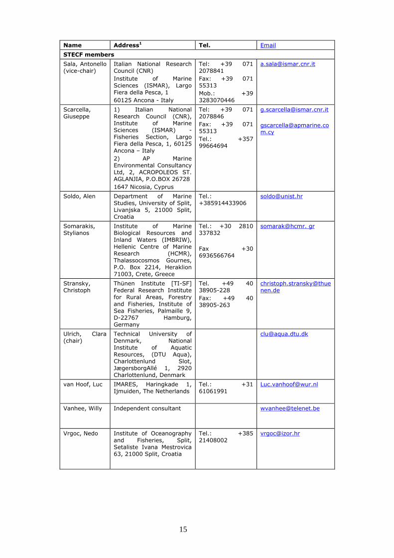
15 15


STECF members

Sala, Antonello (vice-chair)

Italian National Research Council (CNR)

Institute of Marine Sciences (ISMAR), Largo

Fiera della Pesca, 1

60125 Ancona - Italy

Tel: +39 071 2078841

Fax: +39 071 55313

Mob.: +39 3283070446

[email protected]

Scarcella,

Giuseppe

1) Italian National

Research Council (CNR), Institute of Marine Sciences (ISMAR) - Fisheries Section, Largo Fiera della Pesca, 1, 60125 Ancona – Italy

2) AP Marine Environmental Consultancy Ltd, 2, ACROPOLEOS ST. AGLANJIA, P.O.BOX 26728

1647 Nicosia, Cyprus

Tel: +39 071

2078846

Fax: +39 071 55313

Tel.: +357 99664694

[email protected]

[email protected]

Soldo, Alen

Department of Marine Studies, University of Split, Livanjska 5, 21000 Split, Croatia

Tel.: +385914433906

[email protected]

Somarakis, Stylianos

Institute of Marine Biological Resources and Inland Waters (IMBRIW),

Hellenic Centre of Marine Research (HCMR), Thalassocosmos Gournes, P.O. Box 2214, Heraklion 71003, Crete, Greece

Tel.: +30 2810 337832

Fax +30 6936566764

somarak@hcmr. gr

Stransky, Christoph

Thünen Institute [TI-SF] Federal Research Institute for Rural Areas, Forestry

and Fisheries, Institute of Sea Fisheries, Palmaille 9, D-22767 Hamburg, Germany

Tel. +49 40 38905-228

Fax: +49 40

38905-263

[email protected]

Ulrich, Clara (chair)

Technical University of Denmark, National Institute of Aquatic Resources, (DTU Aqua), Charlottenlund Slot,

JægersborgAllé 1, 2920 Charlottenlund, Denmark

[email protected]

van Hoof, Luc IMARES, Haringkade 1,

Ijmuiden, The Netherlands

Tel.: +31

61061991

[email protected]

Vanhee, Willy

Independent consultant [email protected]

Vrgoc, Nedo Institute of Oceanography

and Fisheries, Split, Setaliste Ivana Mestrovica 63, 21000 Split, Croatia

Tel.: +385

21408002

[email protected]








16 16

17 17

EXPERT GROUP REPORT

REPORT TO THE STECF

Report of the ad hoc Expert Group on monitoring the performance of the Common

Fisheries Policy

Ispra, Italy, March-April 2018

This report does not necessarily reflect the view of the STECF and the

European Commission and in no way anticipates the Commission’s future policy in this area

18 18

1 INTRODUCTION

Article 50 of the EU Common Fisheries Policy (REGULATION (EU) No 1380/2013) states:

“The Commission shall report annually to the European Parliament and to the Council on the

progress on achieving maximum sustainable yield and on the situation of fish stocks, as early as possible following the adoption of the yearly Council Regulation fixing the fishing opportunities

available in Union waters and, in certain non-Union waters, to Union vessels.”

To fulfil its obligations to report to the European Parliament and the Council, each year, the

European Commission requests the Scientific, Technical and Economic Committee for Fisheries (STECF) to compute a series of performance indicators and advise on the progress towards the

provisions of Article 50.

In an attempt to make the process of computing each of the indicators consistent and transparent and to take account of issues identified and documented in previous CFP monitoring reports, a

revised protocol was adopted by the STECF in 2017 (Annex I).

An ad hoc Expert Group comprising Experts from the European Commission’s Joint Research

Centre (JRC) was convened during March and April 2018 to compute the performance indicator values according to the agreed protocol (Annex I) and to report to the STECF plenary meeting

scheduled for 09-13 April 2018.

1.1 Terms of Reference to the ad hoc Expert group

The Expert group is requested to report on progress in achieving MSY objectives in line with CFP.

19 19

2 DATA AND METHODS

2.1 Data sources

The data sources used referred to the coastal waters of the EU in FAO areas 27 (Northeast

Atlantic and adjacent Seas) and 37 (Mediterranean and Black Seas). The Mediterranean included GSAs 1, 5, 6, 7, 8, 9, 10, 11, 15, 16, 17, 18, 19, 25 and 29. The NE Atlantic included the ICES

subareas "III", "IV" (excluding Norwegian waters of division IVa), "VI", "VII", "VIII", "IX" and "X".

2.1.1 Stock assessment information

For the Mediterranean region (FAO area 37), the information were extracted from the STECF Mediterranean Expert Working Group repositories (https://stecf.jrc.ec.europa.eu/reports/medbs)

and from the GFCM stock assessment forms (http://www.fao.org/gfcm/data/safs/en ).

For the NE Atlantic (FAO area 27), the information was downloaded from the ICES website

(http://standardgraphs.ices.dk) on the 19th March 2018, comprising the most recent published assessments, carried out up to and including 2017. A thorough process of data quality checks and

corrections was performed to ensure the information downloaded was in agreement with the

summary sheets published online (Annex III).

Table 6.1 shows the URLs for the report or advice summary sheet for each stock.

2.1.2 Management units information

For the NE Atlantic, management units are defined by TACs, annual fishing opportunities for a species or group of species in a Fishing Management Zone (FMZ). The information regarding TACs

in 2016 was downloaded from the FIDES (http://fides3.fish.cec.eu.int/) reporting system. Subsequently, such information was cleaned and processed, to identify the FMZ of relevance to

this work, as well as the ICES rectangles they span to (Gibin, 2017).

2.2 Methods

The methods applied and the definition of the sampling frames followed the protocol (Jardim et.al, 2015) agreed by STECF (2016) and updated following the discussion in STECF (2017a). The

updated protocol is presented in Annex I and the R code used to carry out the analysis in Annex II.

2.3 Points to note

Stocks assessed with biomass dynamics models do not provide a value for FPA, although

they may provide a BPA proxy (0.5 BMSY). Consequently, such stocks cannot be used to

compute the indicators relating to safe biological limits (SBL).

The Generalized Linear Mixed Model (GLMM) uses a shortened time series, starting in

2003, instead of the full time-series of available data. This has the advantage of balancing

the dataset by removing those years with only a low number of assessment estimates, but

it has the disadvantage of excluding data that could improve model fit.

For all stocks managed with a Bescapement strategy, except Bay of Biscay anchovy (ane.27.8)

and Norway pout in the North Sea, Skagerrak and Kattegat (nop-27.3a.4), MSYBescapement

was set by ICES at BPA instead of BMSY.

Norway pout in the North Sea, Skagerrak and Kattegat (nop.27.3a4) uses a probabilistic

method to set the catches: Cy+1=C|(P[SSB<Blim]=0.05). For this stock, the lower

(0.025%) boundary of the SSB confidence interval was compared to Blim.

https://stecf.jrc.ec.europa.eu/reports/medbs

http://www.fao.org/gfcm/data/safs/en

http://standardgraphs.ices.dk/

20 20

Bay of Biscay anchovy (ane.27.8) uses a HCR with Biomass triggers. ICES does not report

reference points other than Blim. The HCR’s upper biomass trigger was used as

MSYBescapement.

ICES is in the process of shifting MSYBtrigger settings to levels which increase the probability

of keeping F at FMSY, making it a good proxy for BMSY. Nevertheless, there are still 40 out of

69 stocks relevant for this exercise, with MSYBtrigger set at BPA.

The GLMM fit within the bootstrap procedure does not converge for all resamples, up to

20% of the fits fail, with the exception of the trend in SSB or biomass index for stocks of

data category 1-3 (relative to 2003) which had 223 over 500 resamples failing. Failed

resamples were excluded when computating model-based indicators.

The 2017 ICES update of eco regions’ definition removed the category ‘widely distributed’ stocks. For compatibility with previous versions of this report, the stocks previously

included in the category ‘widely distributed’ were kept, and renamed ‘Northeast Atlantic’.

2.4 Differences from the 2017 CFP monitoring report (STECF 17-04)

2.4.1 Northeast Atlantic

Stocks with less than five years of data were not included in the analysis.

The CFP requirements indicator was updated, replacing BPA by MSYBtrigger, making it more in line with the CFP regulation and renamed to avoid misleading the readers, to ‘Stocks

with F above/below Fmsy or SSB below/above MSYBtrigger’. Stocks without stock assessment estimates for 2015 and/or 2016 were assigned values

equivalent to 2014 and/or 2015 estimates respectively.

The Northern shrimp stock (pra.27.1-2) was removed from the computation of the indicator F/FMSY outside the EU coastal waters, because the indicator values were heavily

influenced by the outlier behaviour of this stock (STECF, 2017a).

2.4.2 Mediterranean and Black Sea

A new reference list of stocks was adopted in accordance with the revised protocol

adopted by STECF (2017a). The previous reference list (Mannini et al., 2017) was

complemented with stock assessment results for selected additional species established by

the STECF (2017a).

Stocks with less than five years of data were not included in the analysis.

Stocks without stock assessment estimates for 2015 and/or 2016 were assigned values

equivalent to 2014 and/or 2015 estimates respectively.

Because of the changes in data and protocol, the annual indicator values and associate time-series trends for the Mediterranean and Black seas presented in the current report, cannot be

directly compared to those presented in previous CFP monitoring reports.

21 21

3 NORTHEAST ATLANTIC AND ADJACENT SEAS (FAO REGION 27)

3.1 Number of stock assessments to compute CFP performance indicators

The number of stock assessments with estimates of F/FMSY for the years 2003-2016 for FAO

Region 27 are given in Figure 3.1 and by ecoregion in Table 3.1.

The time-series of data available for each year and stock (data categories 1 and 2) is shown in

Figure 3.2. For stocks without estimates in 2016 the estimates of F and SSB were assumed to be the same as 2015. Consequently, the number of stocks included to compute the indicator values

for 2016 was 71.

The stocks, including data category 3, used to compute each indicator are shown in Table 3.2.

Figure 3.1 Number of stocks in the ICES area for which estimates of F/FMSY are available by year.

Table 3.1 Number of stocks in the ICES area for which estimates of F/FMSY are available by ecoregion and year

EcoRegion 2003 2004 2005 2006 2007 2008 2009 2010 2011 2012 2013 2014 2015 2016

ALL 66 65 66 67 67 67 68 67 69 70 71 71 71 66

Baltic Sea 8 8 8 8 8 8 8 8 8 8 8 8 8 8

BoBiscay & Iberia 9 9 9 9 9 9 9 9 9 9 9 9 9 9

Celtic Seas 21 20 21 22 22 22 23 22 23 24 25 25 25 23

Greater North Sea 21 21 21 21 21 21 21 21 22 22 22 22 22 22

Northeast Atlantic 7 7 7 7 7 7 7 7 7 7 7 7 7 4

22 22

Figure 3.2 Time series of stock assessment results in the ICES area for which estimates of F/FMSY are available by year. Blank records indicate no estimate available for stock and year.

23 23

Compared to the dataset used for the 2017 analyses (STECF, 2017b), the analyses presented in

this report include the results from assessments for the following additional stocks of categories 01 and 02:

had-iris (had.27.7a), ple-iris (ple.27.7a), whg-iris (whg.27.7a) and san-ns4 (san.sa.4),

which were upgraded from category 03 in 2016 to category 01 in 2017. her.27.30.31 which appeared in 2017 for the first time, as a result of merging stocks her-

30 and her-31.

Meanwhile, there were some stocks included in the 2017 analyses (STECF 2017b) which were excluded from the present analyses:

her-30 which has now been merged with her-31 into her.27.30.31.

nep-2021 (nep.fu.2021) and nep-2324 (nep.fu.2324) due to having less than five years of data available.

ICES revised the eco-region classification of the stocks. For consistency with the 2017 report

(STECF, 2017b), the widely distributed stocks were kept the same as last year and the stocks of had.27.46a20, pok.27.3a46 and sol.27.7e were kept in the Greater North Sea eco-region.

In total, 71 stocks of categories 01 and 02 were included in the present analysis.

24 24

Table 3.2 Indicators computed for each stocks.

Stock Year

above/below

Fmsy

in/out

SBL

B wrt

MSYBtrigger

or

F wrt FMSY

F/Fmsy

trends

Biomass

trends

SSB/Bpa

trends

Recruitment

trends

Biomass

data

category 1-

3 trends

Biomass

data

category 3

trends

ane.27.8 2016 X

X

X X

ane.27.9a 2016

X X

anf.27.3a46 2016

X X

ank.27.78ab 2015

X X

ank.27.8c9a 2016 X

X X

X

X

aru.27.5b6a 2016

X X

aru.27.6b7-1012 2016

X X

bli.27.5b67 2015 X X X X X X X X

bll.27.3a47de 2016

X X

boc.27.6-8 2016

X X

bss.27.4bc7ad-h 2016

X

bss.27.8ab 2016

X X

cod.27.21 2016

X X

cod.27.22-24 2016 X X X X X X X X

cod.27.25-32 2016

X X

cod.27.47d20 2016 X X X X X X X X

cod.27.6a 2016 X X X X X X X X

cod.27.7a 2016 X X X X X X X X

cod.27.7e-k 2016 X X X X X X X X

dab.27.22-32 2016

X X

dab.27.3a4 2016

X X

dgs.27.nea 2015 X

X

X

X X

fle.27.2223 2016

X X

fle.27.2425 2016

X X

fle.27.2628 2016

X X

fle.27.2729-32 2016

X X

fle.27.3a4 2016

X X

gfb.27.nea 2015

X X

gug.27.3a47d 2016

X X

had.27.46a20 2016 X X X X X X X X

had.27.6b 2016 X X X X X X X X

had.27.7a 2016 X X X X X X X X

had.27.7b-k 2016 X X X X X X X X

her.27.1-24a514a 2016

X

her.27.20-24 2016 X X X X X X X X

her.27.25-2932 2016 X X X X X X X X

her.27.28 2016 X X X X X X X X

her.27.3031 2016 X X X X X X X X

25 25

Stock Year

above/below

Fmsy

in/out

SBL

B wrt

MSYBtrigger

or

F wrt FMSY

F/Fmsy

trends

Biomass

trends

SSB/Bpa

trends

Recruitment

trends

Biomass

data

category 1-

3 trends

Biomass

data

category 3

trends

her.27.3a47d 2016 X X X X X X X X

her.27.6a7bc 2016 X X X X X X X X

her.27.irls 2016 X X X X X X X X

her.27.nirs 2016 X X X X X X X X

hke.27.3a46-8abd 2016 X X X X X X X X

hke.27.8c9a 2016 X X X X X X X X

hom.27.2a4a5b6a7a-ce-k8 2016 X X X X X X X X

hom.27.9a 2016 X X X X X X X X

jaa.27.10a2 2015

X X

ldb.27.8c9a 2016 X X X X X X X X

lem.27.3a47d 2016

X X

lez.27.4a6a 2016 X

X X

X

X

lez.27.6b 2016

X X

lin.27.3a4a6-91214 2016

X X

lin.27.5b 2016

X X

mac.27.nea 2016 X X X X X X X X

meg.27.7b-k8abd 2016 X X X X X X X X

meg.27.8c9a 2016 X X X X X X X X

mon.27.78ab 2015

X X

mon.27.8c9a 2016 X X X X X X X X

mur.27.3a47d 2016

X X

nep.fu.11 2016 X

X

nep.fu.12 2016 X

X

nep.fu.13 2016 X

X

nep.fu.14 2016 X

X

nep.fu.15 2016 X

X

nep.fu.16 2016 X

nep.fu.17 2016 X

X

nep.fu.19 2016 X

X

nep.fu.22 2016 X

X

nep.fu.25 2015

X X

nep.fu.2627 2015

X X

nep.fu.2829 2016

X X

nep.fu.3-4 2016 X

nep.fu.31 2015

X X

nep.fu.6 2016 X

X

nep.fu.7 2016 X

X

nep.fu.8 2016 X

X

nep.fu.9 2016 X

X

nop.27.3a4 2016 X

X X X X

26 26

Stock Year

above/below

Fmsy

in/out

SBL

B wrt

MSYBtrigger

or

F wrt FMSY

F/Fmsy

trends

Biomass

trends

SSB/Bpa

trends

Recruitment

trends

Biomass

data

category 1-

3 trends

Biomass

data

category 3

trends

pil.27.8abd 2016

X X

pil.27.8c9a 2016

X

ple.27.21-23 2016 X X X X X X X X

ple.27.24-32 2016

X X

ple.27.420 2016 X X X X X X X X

ple.27.7a 2016 X X X X X X X X

ple.27.7d 2016 X X X X X X X X

ple.27.7e 2016

X X

ple.27.7fg 2016

X X

ple.27.7h-k 2016

X X

pok.27.3a46 2016 X X X X X X X X

pra.27.4a20 2016 X X X X X X X X

reb.2127.dp 2016

X X

rjc.27.3a47d 2016

X X

rjc.27.8 2015

X X

rjc.27.9a 2015

X X

rjh.27.9a 2015

X X

rjm.27.3a47d 2016

X X

rjm.27.8 2015

X X

rjm.27.9a 2015

X X

rjn.27.3a4 2016

X X

rjn.27.67 2015

X X

rjn.27.8c 2015

X X

rjn.27.9a 2015

X X

rju.27.7de 2015

X X

rng.27.5b6712b 2015 X

X

X

X

san.sa.1r 2016 X

X X X X

san.sa.2r 2016 X

X X X X

san.sa.3r 2016 X

X X X X

san.sa.4 2016 X

X X X X

sbr.27.9 2015

X X

sdv.27.nea 2016

X X

sho.27.67 2016

X X

sho.27.89a 2016

X X

sol.27.20-24 2016 X X X X X X X X

sol.27.4 2016 X X X X X X X X

sol.27.7a 2015 X X X X X X X X

sol.27.7d 2016 X X X X X X X X

sol.27.7e 2016 X X X X X X X X

sol.27.7fg 2016 X X X X X X X X

27 27

Stock Year

above/below

Fmsy

in/out

SBL

B wrt

MSYBtrigger

or

F wrt FMSY

F/Fmsy

trends

Biomass

trends

SSB/Bpa

trends

Recruitment

trends

Biomass

data

category 1-

3 trends

Biomass

data

category 3

trends

sol.27.7h-k 2016

X X

sol.27.8ab 2016 X X X X X X X X

spr.27.22-32 2016 X X X X X X X X

spr.27.4 2016 X

X X X X

syc.27.3a47d 2016

X X

syc.27.67a-ce-j 2016

X X

syc.27.8abd 2016

X X

syc.27.8c9a 2016

X X

tur.27.3a 2016

X X

tur.27.4 2016

X X

usk.27.3a45b6a7-912b 2016

X X

whb.27.1-91214 2016 X X X X X X X X

whg.27.47d 2016 X X X X X X X X

whg.27.6a 2015 X X X X X X X X

whg.27.7a 2016 X X X X X X X X

whg.27.7b-ce-k 2016 X X X X X X X X

wit.27.3a47d 2016

X X

Total 71 46 62 48 54 55 54 121 61

28 28

3.2 Indicators of management performance

3.2.1 Number of stocks by year where fishing mortality exceeded FMSY

Figure 3.3 Number of stocks by year for which fishing mortality (F) exceeded FMSY.

Figure 3.4 Number of stocks by year and ecoregion for which fishing mortality (F) exceeded FMSY.

Table 3.3 Number of stocks by year and ecoregion for which fishing mortality (F) exceeded FMSY.

EcoRegion 2003 2004 2005 2006 2007 2008 2009 2010 2011 2012 2013 2014 2015 2016

ALL 46 45 50 49 51 48 39 39 32 37 28 32 29 29

Baltic Sea 7 6 6 6 6 6 6 6 4 5 3 2 4 4

BoBiscay & Iberia 6 6 7 7 8 6 5 5 5 5 6 6 5 5

Celtic Seas 13 12 14 14 16 16 13 12 10 12 8 8 8 9


Widely distributed 7 5 5 4 4 4 3 4 3 2 2 3 2 2

29 29

3.2.2 Number of stocks by year for which fishing mortality was equal to, or less than FMSY

Figure 3.5 Number of stocks by year for which fishing mortality (F) did not exceed FMSY.

Figure 3.6 Number of stocks by year and ecoregion for which fishing mortality (F) did not exceed FMSY.

Table 3.4 Number of stocks by year and ecoregion for which fishing mortality (F) did not exceed

FMSY.

EcoRegion 2003 2004 2005 2006 2007 2008 2009 2010 2011 2012 2013 2014 2015 2016

ALL 20 20 16 18 16 19 29 28 37 33 43 39 42 42

Baltic Sea 1 2 2 2 2 2 2 2 4 3 5 6 4 4

BoBiscay & Iberia 3 3 2 2 1 3 4 4 4 4 3 3 4 4

Celtic Seas 8 8 7 8 6 6 10 10 13 12 17 17 17 16



30 30

3.2.3 Number of stocks outside safe biological limits

Figure 3.7 Number of stocks outside safe biological limits by year.

Figure 3.8 Number of stocks outside safe biological limits by ecoregion and year.

Table 3.5 Number of stocks outside safe biological limits by ecoregion and year.

EcoRegion 2003 2004 2005 2006 2007 2008 2009 2010 2011 2012 2013 2014 2015 2016

ALL 31 31 32 29 29 26 21 20 22 20 17 21 18 16

Baltic Sea 6 6 6 5 5 5 5 5 5 4 4 4 3 3

BoBiscay & Iberia 4 4 5 5 4 3 3 1 1 2 1 2 3 0

Celtic Seas 11 11 10 8 9 9 8 8 8 9 9 9 7 9



31 31

3.2.4 Number of stocks inside safe biological limits

Figure 3.9 Number of stocks inside safe biological limits by year.

Figure 3.10 Number of stocks inside safe biological limits by ecoregion and year.

Table 3.6 Number of stocks inside safe biological limits by ecoregion and year.

EcoRegion 2003 2004 2005 2006 2007 2008 2009 2010 2011 2012 2013 2014 2015 2016

ALL 15 15 14 17 17 20 25 26 24 26 29 25 28 30

Baltic Sea 2 2 2 3 3 3 3 3 3 4 4 4 5 5

BoBiscay & Iberia 3 3 2 2 3 4 4 6 6 5 6 5 4 7

Celtic Seas 4 4 5 7 6 6 7 7 7 6 6 6 8 6



32 32

3.2.5 Trend in F/FMSY

Indicators of trends show the average progress of the process they represent, including its

uncertainty in terms of 50% and 95% confidence intervals. In the former case corresponding to the range between the 25% and 75% percentiles, and for the latter between the 2.5% and

97.5% percentiles.

Trends in F/FMSY by ecoregion and year are given in Figure 3.11 and the associated percentiles are

given in Table 3.7. Figure 3.11 shows the indicator value in 2016 close to 1, which means that over all stocks, on average, the exploitation levels are close to FMSY. Nevertheless, there are still

about 40% of the stocks which are being exploited above FMSY (see sections 3.2.1 and 3.2.2).

Figure 3.11 Trend in F/FMSY. Dark grey zone shows the 50% confidence interval; the light grey zone

shows the 95% confidence interval.

Table 3.7 Percentiles for F/FMSY by year.

2003 2004 2005 2006 2007 2008 2009 2010 2011 2012 2013 2014 2015 2016

2.5% 1.42 1.40 1.36 1.32 1.28 1.17 1.06 1.00 0.90 0.89 0.82 0.89 0.86 0.84

25% 1.55 1.53 1.48 1.45 1.42 1.27 1.17 1.11 1.00 0.99 0.92 1.02 0.98 0.93

50% 1.64 1.61 1.55 1.52 1.48 1.34 1.23 1.17 1.05 1.04 0.97 1.07 1.03 0.98

75% 1.71 1.69 1.63 1.58 1.55 1.41 1.30 1.23 1.10 1.09 1.01 1.13 1.08 1.03

97.5% 1.87 1.85 1.77 1.70 1.68 1.52 1.41 1.33 1.21 1.20 1.14 1.26 1.20 1.15

33 33

Trends in F/FMSY by ecoregion are given in Figure 3.13 and Table 3.8. The regional analysis was

carried out using the same model applied to regional datasets. Due to the small number of stocks in each ecoregion it was not possible to compute confidence intervals.

Figure 3.12 Trend in F/FMSY by ecoregion.

Table 3.8. Trend in F/FMSY by ecoregion and year

EcoRegion 2003 2004 2005 2006 2007 2008 2009 2010 2011 2012 2013 2014 2015 2016

ALL 1.64 1.61 1.55 1.52 1.48 1.34 1.23 1.17 1.05 1.04 0.97 1.07 1.03 0.98

Baltic Sea 1.60 1.63 1.57 1.51 1.51 1.45 1.41 1.27 1.16 1.07 1.07 1.05 1.12 1.18

BoBiscay & Iberia 1.36 1.35 1.44 1.58 1.46 1.27 1.21 1.05 1.10 1.10 1.08 1.21 1.20 0.98

Celtic Seas 1.94 1.93 1.78 1.63 1.66 1.52 1.38 1.38 1.10 1.14 0.90 1.08 0.95 0.89

Greater North Sea 1.47 1.45 1.39 1.44 1.36 1.20 1.06 1.01 1.03 0.99 0.97 1.03 1.00 0.99

Widely distributed 1.64 1.48 1.44 1.33 1.25 1.10 0.99 0.94 0.74 0.75 0.81 0.93 0.94 0.90

34 34

3.2.6 Trend in SSB (relative to 2003)



97.5% percentiles.

Figure 3.13 and Table 3.9 present the evolution of SSB over the period of the study, scaled to the

initial (2003) value for presentation purposes. Over the time series, SSB shows a generally increasing pattern.

Figure 3.13 Trend in SSB relative to 2003. Dark grey zone shows the 50% confidence interval; the light

grey zone shows the 95% confidence interval.

Table 3.9 Percentiles for SSB by year relative to 2003.

2003 2004 2005 2006 2007 2008 2009 2010 2011 2012 2013 2014 2015 2016

2.5% 0.66 0.60 0.57 0.55 0.55 0.59 0.62 0.67 0.80 0.75 0.72 0.76 0.83 0.92

25% 0.86 0.79 0.75 0.73 0.73 0.78 0.80 0.86 1.06 0.99 0.94 1.00 1.09 1.19

50% 1.00 0.92 0.87 0.84 0.84 0.90 0.92 1.00 1.23 1.14 1.10 1.16 1.26 1.39

75% 1.17 1.07 1.03 1.00 0.99 1.06 1.09 1.18 1.42 1.32 1.27 1.34 1.46 1.60

97.5% 1.47 1.37 1.32 1.30 1.31 1.37 1.40 1.54 1.87 1.77 1.70 1.80 1.97 2.12

35 35

Trends in SSB by ecoregion and year are given in Figure 3.14 and Table 3.10. The regional

analysis was carried out using the same model applied to regional datasets. Due to the small

number of stocks in each ecoregion it wasn’t possible to compute confidence intervals.

Figure 3.14 Trend in SSB by ecoregion relative to 2003.

Table 3.10 SSB relative to 2003 by ecoregion.

EcoRegion 2003 2004 2005 2006 2007 2008 2009 2010 2011 2012 2013 2014 2015 2016

ALL 1.00 0.92 0.87 0.84 0.84 0.90 0.92 1.00 1.23 1.14 1.10 1.16 1.26 1.39

Baltic Sea 1.00 1.07 1.17 1.17 1.11 1.00 0.99 1.01 0.98 1.03 1.08 1.21 1.20 1.22

BoBiscay & Iberia 1.00 1.04 1.02 1.06 1.08 1.08 1.13 1.26 1.57 1.55 1.42 1.60 1.72 1.80

Celtic Seas 1.00 0.87 0.73 0.70 0.71 0.78 0.76 0.78 0.95 0.98 0.90 0.87 1.10 1.21

Greater North Sea 1.00 0.83 0.80 0.72 0.75 0.89 0.95 1.08 1.45 1.14 1.10 1.20 1.24 1.47

Widely distributed 1.00 1.05 1.06 1.06 1.04 1.04 1.07 1.18 1.34 1.40 1.40 1.43 1.51 1.54

36 36

3.3 Experimental indicators

STECF (2017a) required a list of experimental indicators to be computed, similar to the 2017 exercise

(STECF, 2017b). The estimates obtained for these indicators are not stable and should be considered

with care.

37 37

3.3.1 Number of stocks with F above Fmsy or SSB below MSYBtrigger

Figure 3.15 Number of stocks with F above Fmsy or SSB below MSYBtrigger by year.

Figure 3.16 Number of stocks with F above Fmsy or SSB below MSYBtrigger by ecoregion and year.

Table 3.11 Number of stocks with F above Fmsy or SSB below MSYBtrigger by ecoregion and year.

EcoRegion 2003 2004 2005 2006 2007 2008 2009 2010 2011 2012 2013 2014 2015 2016

ALL 43 44 47 46 48 47 42 41 40 42 32 35 36 37

Baltic Sea 7 7 7 6 6 6 6 6 6 6 4 4 5 5

BoBiscay & Iberia 6 7 7 7 7 6 6 6 6 6 6 5 5 5

Celtic Seas 14 13 15 14 16 17 15 13 12 16 13 12 12 14



38 38

3.3.2 Number of stocks with F below or equal to Fmsy and SSB above or equal to MSYBtrigger

Figure 3.17 Number of stocks with F below or equal to Fmsy and SSB above or equal to MSYBtrigger.

Figure 3.18 Number of stocks with F below or equal to Fmsy and SSB above or equal to MSYBtrigger by

ecoregion and year.

Table 3.12 Number of stocks with F below or equal to Fmsy and SSB above or equal to MSYBtrigger by

ecoregion and year.

EcoRegion 2003 2004 2005 2006 2007 2008 2009 2010 2011 2012 2013 2014 2015 2016

ALL 16 14 12 14 12 13 19 19 21 19 30 27 26 25

Baltic Sea 1 1 1 2 2 2 2 2 2 2 4 4 3 3

BoBiscay & Iberia 2 1 1 1 1 2 2 2 2 2 2 3 3 3

Celtic Seas 7 7 6 8 6 5 8 9 11 7 11 12 12 10



39 39

3.3.3 Trend in F/FMSY for stocks outside the EU coastal waters



97.5% percentiles.

This indicator was based on 9 stocks. The Northern shrimp stock (pra.27.1-2) was removed from

the computation of the indicator F/FMSY outside the EU coastal waters, because the indicator values were heavily influenced by the outlier behaviour of this stock (STECF, 2017a).

Figure 3.19 Trend in F/FMSY for stocks outside the EU coastal waters. Dark grey zone shows the 50%

confidence interval; the light grey zone shows the 95% confidence interval.

Table 3.13 Percentiles for F/FMSY for stocks outside the EU coastal waters by year.

2003 2004 2005 2006 2007 2008 2009 2010 2011 2012 2013 2014 2015 2016

2.5% 1.24 1.21 1.30 1.16 1.16 1.13 0.91 0.94 0.89 0.92 0.84 0.81 0.84 0.86

25% 1.44 1.40 1.50 1.35 1.31 1.31 1.09 1.14 1.05 1.07 0.98 0.94 0.98 0.98

50% 1.55 1.52 1.62 1.47 1.41 1.40 1.19 1.25 1.15 1.17 1.06 1.03 1.07 1.06

75% 1.67 1.66 1.73 1.58 1.50 1.49 1.32 1.40 1.26 1.27 1.15 1.13 1.17 1.14

97.5% 1.89 1.98 2.02 1.87 1.72 1.75 1.56 1.65 1.47 1.47 1.37 1.40 1.42 1.35

40 40

3.3.4 Trend in SSB/Bpa


uncertainty in terms of 50% and 95% confidence intervals. In the former case corresponding to the range between the 25% and 75% percentiles, and for the last between the 2.5% and 97.5%

percentiles.

Figure 3.20 Trend in SSB/Bpa. Dark grey zone shows the 50% confidence interval; the light grey zone


Table 3.14 Percentiles for SSB/Bpa by year.

2003 2004 2005 2006 2007 2008 2009 2010 2011 2012 2013 2014 2015 2016

2.5% 0.87 0.78 0.76 0.73 0.73 0.78 0.79 0.85 0.98 0.95 0.92 0.96 1.05 1.15

25% 0.95 0.88 0.84 0.81 0.81 0.87 0.89 0.95 1.12 1.07 1.04 1.10 1.19 1.31

50% 1.02 0.94 0.90 0.87 0.87 0.93 0.95 1.02 1.20 1.15 1.12 1.17 1.27 1.40

75% 1.07 1.00 0.96 0.92 0.92 0.99 1.01 1.08 1.30 1.22 1.19 1.25 1.36 1.51

97.5% 1.20 1.10 1.09 1.05 1.05 1.12 1.15 1.25 1.50 1.40 1.36 1.43 1.54 1.70

41 41

3.3.5 Trend in recruitment (relative to 2003)



97.5% percentiles.

Figure 3.21 Trend in R/R2003 . Dark grey zone shows the 50% confidence interval; the light grey zone


Table 3.15 Percentiles for R/R2003 by year.

2003 2004 2005 2006 2007 2008 2009 2010 2011 2012 2013 2014 2015 2016

2.5% 0.49 0.50 0.48 0.52 0.45 0.43 0.59 0.53 0.48 0.47 0.52 0.62 0.55 0.59

25% 0.79 0.75 0.76 0.83 0.70 0.70 0.99 0.80 0.76 0.73 0.82 0.98 0.88 0.94

50% 1.00 0.94 0.96 1.06 0.90 0.89 1.30 1.01 0.96 0.94 1.06 1.27 1.11 1.26

75% 1.28 1.19 1.23 1.32 1.12 1.12 1.71 1.25 1.20 1.22 1.34 1.62 1.41 1.64

97.5% 1.96 1.76 1.88 1.98 1.69 1.75 2.70 1.88 1.78 1.80 2.00 2.66 2.12 2.67

42 42

3.3.6 Trend in SSB or biomass index for stocks of data category 1-3 (relative to 2003)



97.5% percentiles.

Note that the bootstrap procedure failed in 223 over 500 iterations, which is a sign of the poor fit

of the model to the dataset. It also explains the value of 0.96 in 2003 (Table 3.16), which derives from the skewed distribution obtained for this indicator.

Figure 3.22 Trend in SSB relative to 2003 for category 1-3 stocks. Dark grey zone shows the 50%


Table 3.16 Percentiles for SSB relative to 2003 by year for category 1-3 stocks.

2003 2004 2005 2006 2007 2008 2009 2010 2011 2012 2013 2014 2015 2016

2.5% 0.49 0.45 0.45 0.46 0.50 0.53 0.53 0.58 0.63 0.62 0.62 0.64 0.73 0.77

25% 0.77 0.73 0.72 0.74 0.76 0.82 0.79 0.83 0.91 0.97 0.94 0.99 1.14 1.20

50% 0.96 0.93 0.91 0.95 0.99 1.03 1.01 1.08 1.19 1.25 1.22 1.28 1.48 1.54

75% 1.30 1.23 1.23 1.26 1.29 1.37 1.34 1.43 1.60 1.65 1.61 1.69 1.93 2.06

97.5% 2.12 2.00 1.95 1.96 2.01 2.09 2.09 2.22 2.46 2.55 2.47 2.72 3.06 3.35

43 43

3.3.7 Trend in SSB or biomass index for stocks of data category 3 (relative to 2003)



97.5% percentiles.

Figure 3.23 Trend in SSB relative to 2003 for category 3 stocks. Dark grey zone shows the 50%


Table 3.17 Percentiles for SSB relative to 2003 by year for category 3 stocks.

2003 2004 2005 2006 2007 2008 2009 2010 2011 2012 2013 2014 2015 2016

2.5% 0.59 0.62 0.63 0.66 0.73 0.75 0.71 0.76 0.77 0.90 0.89 0.93 1.08 1.11

25% 0.82 0.84 0.84 0.92 0.99 1.04 0.99 1.04 1.09 1.24 1.23 1.29 1.53 1.56

50% 1.01 1.02 1.03 1.10 1.18 1.27 1.18 1.25 1.29 1.47 1.47 1.55 1.85 1.87

75% 1.21 1.19 1.18 1.29 1.37 1.50 1.40 1.47 1.52 1.74 1.72 1.82 2.15 2.21

97.5% 1.80 1.74 1.74 1.92 2.03 2.13 2.01 2.09 2.18 2.57 2.52 2.64 3.12 3.22

44 44

3.4 Indicators of advice coverage

The indicator of advice coverage computes the number of stocks for which the reference points,

FMSY, FPA, MSYBtrigger and BPA are available and the number of associated TACs. Note that provided part of a given TAC management area overlaps with part of a stock assessment area, the setting

of the TAC is considered as being based on the relevant stock assessment. Consequently, the advice coverage indicator is biased upwards if compared with the full spatial coverage of TAC

areas by stock assessments.

Table 3.18 Coverage of TACs by scientific advice (ICES categories 1+2).

No of

stocks

No of

TACs

No of TACs based on

stock assessments

Fraction of TACs based on

stock assessments

Fmsy 71 156 87 0.56

MSYBtrigger 69 156 86 0.55

Fpa 46 156 72 0.46

Bpa 55 156 79 0.51

45 45

4 MEDITERRANEAN AND BLACK SEAS (FAO REGION 37)

There was a strong increasing trend in the number of stocks assessed for years 2003-2009, from 22 up to 47; the number of stock assessments kept stable until 2014 and decreased to 39 in

2015 and 21 in 2016 (Figure 4.1 and Figure 4.2).

This situation renders the interpretation of the deterministic indicators misleading. With such

differences in the number of stocks assessed each year, the trends in the indicators are confounded with the number of stocks available for their computation. Consequently, only the

model-based indicators are shown.

Nevertheless, the indicator values presented (Figure 4.3 and Figure 4.4) are not very robust due

to the large changes in the number of stocks available to fit the model, and therefore the results

should be interpreted with caution.

Figure 4.1 indicates by year, the number of stocks in the Mediterranean and Black Seas for which

estimates of F/FMSY are available. The major reduction in 2016 is due to:

the STECF EWG part I carried out analytical assessments for only 8 out of 11 stocks

(STECF 2017c).

the STECF EWG part II carried out analytical assessment for 5 out of 19 stocks (STECF,

2018).

GFCM assessments performed in 2017 in WGSASP and WGSADM have not yet been

reviewed and approved by the GFCM Scientific Advisory Committee. Consequently, they

were not included in the present analysis.

Table 4.1 shows the stocks added to the current exercise.

Since there are no results for 2016 for any of the GFCM stock assessments and the indicator values for 2016 are based on the results of only 21 stock assessments, such values are not

comparable with those for earlier years of the time-series. Hence in Figure 4.1, the 2016 value is

represented as stand-alone, and the indicators are plotted up to 2015 only.

Figure 4.1 Number of stock assessments in the Mediterranean and Black Sea by year. The totals include stocks in the following GSAs only: 1, 5-7, 9, 10-19, 22-23, 25 and 29.

46 46

Figure 4.2 Time-series of stock assessments available from both STECF and GFCM for computation of model based CFP monitoring indicators for Mediterranean and Black Seas. The red

line indicates that only stock assessment results up to and including 2015 have been used to

compute the indicator values.

47 47

Table 4.1 Stocks added to the current exercise with relation to previous report.

EcoRegion Year Stock Description Updated New Source

Black sea 2014 ane_29 European anchovy in GSA 29 2016 N STECF

Black sea 2014 dgs_29 Picked dogfish in GSA 29 2016 N STECF

Black sea 2014 hmm_29 Mediterranean horse mackerel in GSA 29 2016 N STECF

Black sea 2014 mut_29 Red mullet in GSA 29 2016 N STECF

Black sea 2016 rpw_29 Rapana whelk in GSA 29 2016 Y STECF

Black sea 2014 tur_29 Turbot in GSA 29 2016 N STECF

Black sea 2014 spr_29 Sprattus sprattus in GSA 29 2016 N STECF

Black sea 2016 whg_29 Whiting in GSA 29 2016 Y STECF

Central Med. 2015 ane_17_18 European anchovy in GSA 17, 18 2016 N STECF

Central Med. 2015 nep_17_18 Nephrops in GSA 17, 18 2016 N STECF

Central Med. 2015 pil_17_18 European pilchard(=Sardine) in GSA 17, 18 2016 N STECF

Central Med. 2014 ars_18_19 Giant red shrimp in GSA 18, 19 2014 N STECF

Central Med. 2014 dps_17_18_19 Deep-water rose shrimp in GSA 17, 18, 19 2016 N STECF

Central Med. 2014 hke_17_18 European hake in GSA 17, 18 2014 N STECF

Central Med. 2014 hke_19 European hake in GSA 19 2016 N STECF

Central Med. 2014 mts_17_18 Spottail mantis squillid in GSA 17, 18 2016 N STECF

Central Med. 2014 mut_17_18 Red mullet in GSA 17, 18 2014 N STECF

Central Med. 2014 sol_17 Common sole in GSA 17 2014 N STECF

Central Med. 2015 mut_15_16 Red mullet in GSA 15,16 2015 Y GFCM

Central Med. 2016 mut_19 Red mullet in GSA 19 2016 Y STECF

Central Med. 2014 hke_12_13_14_15_16 Merluccius merluccius in GSA 12, 13, 14, 15, 16 2015 N GFCM

Central Med. 2014 dps_12_13_14_15_16 Parapenaeus longirostris in GSA 12, 13, 14, 15, 16 2015 N GFCM

Eastern Med. 2016 ane_22_23 European anchovy in GSA 22, 23 2016 Y STECF

Eastern Med. 2016 pil_22_23 European pilchard(=Sardine) in GSA 22, 23 2016 Y STECF

Eastern Med. 2014 mut_25 Mullus barbatus in GSA 25 2015 N GFCM

Western Med. 2016 ane_09_10_11 European anchovy in GSA 09, 10, 11 2016 Y STECF

Western Med. 2015 ane_6 Anchovy in GSA 6 2016 N STECF

Western Med. 2015 dps_1 Deep-water rose shrimp in GSA 1 2015 N STECF

Western Med. 2015 mut_7 Red mullet in GSA 7 2015 Y GFCM

Western Med. 2015 dps_09_10_11 Deep-water rose shrimp in GSA 09, 10, 11 2015 N STECF

Western Med. 2015 mur_9 Surmullet in GSA 9 2015 N STECF

Western Med. 2015 ara_9 Blue and red shrimp in GSA 9 2015 Y GFCM

Western Med. 2015 ars_9 Giant red shrimp in GSA 9 2015 Y GFCM

Western Med. 2015 nep_9 Norway lobster in GSA 9 2015 N STECF

Western Med. 2015 nep_6 Norway lobster in GSA 6 2015 N STECF

Western Med. 2015 nep_11 Norway lobster in GSA 11 2015 Y STECF

Western Med. 2015 ara_1 Blue and red shrimp in GSA 1 2015 Y GFCM

Western Med. 2015 mur_5 Striped red mullet in GSA 5 2015 Y GFCM

Western Med. 2015 pil_6 European pilchard(=Sardine) in GSA 6 2016 N STECF

Western Med. 2014 ara_6 Blue and red shrimp in GSA 6 2015 N GFCM

Western Med. 2014 ars_10 Giant red shrimp in GSA 10 2014 N STECF

Western Med. 2014 ars_11 Giant red shrimp in GSA 11 2014 N STECF

Western Med. 2014 hke_01_05_06_07 European hake in GSA 01, 05, 06, 07 2014 N STECF

Western Med. 2014 hke_09_10_11 European hake in GSA 09, 10, 11 2014 N STECF

Western Med. 2016 hom_09_10_11 Atlantic horse mackerel in GSA 09, 10, 11 2016 Y STECF

Western Med. 2013 mut_6 Red mullet in GSA 6 2015 N GFCM

Western Med. 2013 ara_5 Aristeus antennatus in GSA 5 2015 N GFCM

48 48

4.1 Indicators of management performance

4.1.1 Trend in F/FMSY

Indicators of trends show the average progress of the process they represent, including its uncertainty in terms of 50% and 95% confidence intervals. In the former case corresponding to

the range between the 25% and 75% percentiles, and for the latter between the 2.5% and 97.5% percentiles.

Figure 4.3 Trend in F/FMSY. Dark grey zone shows the 50% confidence interval; the light grey

zone shows the 95% confidence interval.

Table 4.2 Percentiles for F/FMSY by year.

2003 2004 2005 2006 2007 2008 2009 2010 2011 2012 2013 2014 2015

2.50% 1.73 1.82 1.87 1.94 1.80 1.85 1.87 1.88 2.11 1.94 1.95 1.81 1.88

25% 2.00 2.07 2.16 2.22 2.06 2.06 2.08 2.10 2.35 2.14 2.13 2.03 2.10

50% 2.17 2.23 2.34 2.37 2.18 2.19 2.19 2.22 2.49 2.28 2.27 2.15 2.25

75% 2.36 2.37 2.52 2.52 2.32 2.33 2.33 2.36 2.64 2.42 2.38 2.30 2.40

97.50% 2.72 2.67 2.86 2.81 2.57 2.59 2.58 2.59 2.92 2.68 2.63 2.59 2.72

The model used is a mixed linear model, described in the protocol (Annex I). Values for 2016 were removed from the model fit. Bootstrapped quantiles of F/FMSY are displayed (Figure 4.3 and

Table 4.1). The 50% quantile (black line), which is equivalent to the median, shows a median

level slightly varying around of F/FMSY ≈ 2.3 for the full time series. In the Mediterranean and Black Seas assessments, a more conservative proxy for FMSY, such as F0.1, is commonly used

resulting in a higher ratio for F/FMSY. The lower quantile is above F/FMSY = 1, indicating that the stocks are exploited well above the CFP management objectives. There is no trend, to indicate

any improvement in exploitation since the implementation of the 2003 reform of the CFP.

49 49

4.1.2 Trend in SSB (relative to 2003)



97.5% percentiles.

Figure 4.4 Trend in SSB relative to 2003. Dark grey zone shows the 50% confidence interval; the light grey zone shows the 95% confidence interval.

Table 4.3 Percentiles for SSB by year relative to 2003.

2003 2004 2005 2006 2007 2008 2009 2010 2011 2012 2013 2014 2015

2.50% 0.58 0.53 0.55 0.63 0.57 0.54 0.57 0.58 0.57 0.53 0.53 0.57 0.58

25% 0.84 0.79 0.79 0.91 0.85 0.77 0.82 0.82 0.79 0.75 0.75 0.80 0.81

50% 1.01 0.95 0.94 1.07 1.00 0.91 0.96 0.97 0.93 0.87 0.89 0.96 0.97

75% 1.18 1.10 1.12 1.25 1.15 1.08 1.14 1.12 1.08 1.02 1.03 1.10 1.12

97.5% 1.73 1.66 1.66 1.87 1.76 1.58 1.66 1.63 1.56 1.44 1.52 1.67 1.75

The 50% quantile (black line), has varied around B/B2003≈ 0.95 (only in 2006 was the ratio above

1.0). However, the quantiles are large, representing a high level of uncertainty.

50 50

4.2 Indicators of advice coverage

In the Mediterranean and the Black Seas a total of 241 stocks were considered for the current

exercise, of which 72 have stock assessments carried out between 2015-2017. The advice coverage for the Mediterranean and the Black Sea is 0.30.

51 51

5 STATUS ACROSS ALL STOCKS IN 2016

Table 5.1 Stock status for all stocks in the analysis. Columns refer to ecoregion, last year for which the estimated was obtained, stock code and description,

value of F/FMSY ratio (F ind), if F is lower than FMSY (F status), if the stock is inside safe biological limits (SBL), and if the stock is inside the CFP

requirements (CFP). Stocks managed under escapement strategies dot not have an estimate of F/FMSY. Symbol ‘o’ stands for ‘YES’, an empty cell stands for

‘NO’ and ‘-’ unknown due to missing information.

Region EcoRegion Year Stock Description F ind

F

status SBL

FAO37 Black Sea 2015 ane_29 European anchovy in GSA 29 1.46 -

FAO37 Black Sea 2015 dgs_29 Piked dogfish in GSA 29 19.05 -

FAO37 Black Sea 2015 hmm_29 Horse mackerel in GSA 29 3.39 -

FAO37 Black Sea 2015 mut_29 Red mullet in GSA 29 0.88 o -

FAO37 Black Sea 2015 whg_29 Whiting in GSA 29 2.14 -

FAO37 Black Sea 2015 tur_29 Turbot in GSA 29 2.81 -

FAO37 Black Sea 2015 spr_29 European sprat in GSA 29 1.82 -

FAO37 Black Sea 2015 rpw_29 Rapana whelk in GSA 29 1.93 -

FAO37 Central Med. 2014 sol_17 Common sole in GSA 17 2.44 -

FAO37 Central Med. 2015 hke_19 European hake in GSA 19 10.43 -

FAO37 Central Med. 2015 mut_19 Red mullet in GSA 19 2.72 -

FAO37 Central Med. 2015 ane_17_18 European anchovy in GSA 17, 18 2.49 -

FAO37 Central Med. 2015 pil_17_18 Sardine in GSA 17, 18 3.18 -

FAO37 Central Med. 2015 nep_17_18 Norway lobster in GSA 17, 18 1.49 -

FAO37 Central Med. 2014 hke_17_18 European hake in GSA 17, 18 5.57 -

FAO37 Central Med. 2015 mts_17_18 Spottail mantis shrimp in GSA 17, 18 2.20 -

FAO37 Central Med. 2015 dps_17_18_19 Deep-water rose shrimp in GSA 17, 18, 19 2.06 -

FAO37 Central Med. 2014 ars_18_19 Giant red shrimp in GSA 18, 19 1.10 -

FAO37 Central Med. 2014 mut_17_18 Red mullet in GSA 17, 18 1.32 -

FAO37 Central Med. 2015 hke_12_13_14_15_16 European hake in GSA 12, 13, 14, 15, 16 6.83 -

FAO37 Central Med. 2015 dps_12_13_14_15_16 Deep water rose shrimp in GSA 12, 13, 14, 15, 16 1.44 -

FAO37 Central Med. 2015 mut_15_16 Red mullet in GSA 15, 16 1.71 -

FAO37 Eastern Med. 2015 ane_22_23 European anchovy in GSA 22, 23 1.30 -

FAO37 Eastern Med. 2015 pil_22_23 Sardine in GSA 22, 23 1.39 -

FAO37 Eastern Med. 2015 mut_25 Red mullet in GSA 25 1.03 -

FAO37 Western Med. 2015 dps_1 Deep-water rose shrimp in GSA 1 0.90 o -

FAO37 Western Med. 2015 dps_09_10_11 Deep-water rose shrimp in GSA 09, 10, 11 0.95 o -

FAO37 Western Med. 2015 mur_9 Striped red mullet in GSA 9 0.95 o -

FAO37 Western Med. 2015 nep_9 Norway lobster in GSA 9 1.78 -



FAO37 Western Med. 2015 ane_6 European anchovy in GSA 6 1.17 -

FAO37 Western Med. 2015 pil_6 Sardine in GSA 6 1.73 -

FAO37 Western Med. 2015 ane_09_10_11 European anchovy in GSA 09, 10, 11 2.04 -

FAO37 Western Med. 2015 hom_09_10_11 Atlantic horse mackerel in GSA 09, 10, 11 3.78 -

FAO37 Western Med. 2015 ars_9 Giant red shrimp in GSA 9 0.78 o -

52 52


F

status SBL

FAO37 Western Med. 2015 ara_5 Blue and red shrimp in GSA 5 1.01 -


FAO37 Western Med. 2015 ara_9 Blue and red shrimp in GSA 9 0.84 o -

FAO37 Western Med. 2015 mut_6 Red mullet in GSA 6 1.56 -

FAO37 Western Med. 2015 mut_7 Red mullet in GSA 7 2.26 -

FAO37 Western Med. 2015 mur_5 Striped red mullet in GSA 5 3.51 -


FAO37 Western Med. 2014 ars_10 Giant red shrimp in GSA 10 1.40 -

FAO37 Western Med. 2014 ars_11 Giant red shrimp in GSA 11 1.60 -

FAO37 Western Med. 2014 hke_01_05_06_07 European hake in GSA 01, 05, 06, 07 2.88 -

FAO37 Western Med. 2014 hke_09_10_11 European hake in GSA 09, 10, 11 5.26 -

FAO27 Baltic Sea 2016 cod.27.22-24 Cod (Gadus morhua) in subdivisions 22-24. western Baltic stock (western Baltic Sea) 3.58

FAO27 Baltic Sea 2016 her.27.20-24 Herring (Clupea harengus) in subdivisions 20-24. spring spawners (Skagerrak. Kattegat. and

western Baltic) 1.27

FAO27 Baltic Sea 2016 her.27.25-2932 Herring (Clupea harengus) in subdivisions 25-29 and 32. excluding the Gulf of Riga (central

Baltic Sea) 0.92 o o

FAO27 Baltic Sea 2016 her.27.28 Herring (Clupea harengus) in Subdivision 28.1 (Gulf of Riga) 1.25 o

FAO27 Baltic Sea 2016 her.27.3031 Herring (Clupea harengus) in subdivisions 30 and 31 (Gulf of Bothnia) 1.10 o

FAO27 Baltic Sea 2016 ple.27.21-23 Plaice (Pleuronectes platessa) in subdivisions 21-23 (Kattegat. Belt Seas. and the Sound) 0.76 o o

FAO27 Baltic Sea 2016 sol.27.20-24 Sole (Solea solea) in subdivisions 20-24 (Skagerrak and Kattegat. western Baltic Sea) 0.75 o

FAO27 Baltic Sea 2016 spr.27.22-32 Sprat (Sprattus sprattus) in subdivisions 22-32 (Baltic Sea) 0.86 o o

FAO27 BoBiscay & Iberia 2016 ane.27.8 Anchovy (Engraulis encrasicolus) in Subarea 8 (Bay of Biscay) - o -

FAO27 BoBiscay & Iberia 2016 ank.27.8c9a Black-bellied anglerfish (Lophius budegassa) in divisions 8.c and 9.a (Cantabrian Sea. Atlantic

Iberian waters) 0.45 o -

FAO27 BoBiscay & Iberia 2016 hke.27.8c9a Hake (Merluccius merluccius) in divisions 8.c and 9.a. Southern stock (Cantabrian Sea and

Atlantic Iberian waters) 2.27

o

FAO27 BoBiscay & Iberia 2016 hom.27.9a Horse mackerel (Trachurus trachurus) in Division 9.a (Atlantic Iberian waters) 0.70 o o

FAO27 BoBiscay & Iberia 2016 ldb.27.8c9a Four-spot megrim (Lepidorhombus boscii) in divisions 8.c and 9.a (southern Bay of Biscay and

Atlantic Iberian waters East) 1.14

o

FAO27 BoBiscay & Iberia 2016 meg.27.7b-k8abd Megrim (Lepidorhombus whiffiagonis) in divisions 7.b-k. 8.a-b. and 8.d (west and southwest of

Ireland. Bay of Biscay) 1.14 o

FAO27 BoBiscay & Iberia 2016 meg.27.8c9a Megrim (Lepidorhombus whiffiagonis) in divisions 8.c and 9.a (Cantabrian Sea and Atlantic

Iberian waters) 1.11 o

FAO27 BoBiscay & Iberia 2016 mon.27.8c9a White anglerfish (Lophius piscatorius) in divisions 8.c and 9.a (Cantabrian Sea and Atlantic

Iberian waters) 0.68 o o

FAO27 BoBiscay & Iberia 2016 sol.27.8ab Sole (Solea solea) in divisions 8.a-b (northern and central Bay of Biscay) 1.10

o

FAO27 Celtic Seas 2016 cod.27.6a Cod (Gadus morhua) in Division 6.a (West of Scotland) 5.65

FAO27 Celtic Seas 2016 cod.27.7a Cod (Gadus morhua) in Division 7.a (Irish Sea) 0.09 o

FAO27 Celtic Seas 2016 cod.27.7e-k Cod (Gadus morhua) in divisions 7.e-k (eastern English Channel and southern Celtic Seas) 1.24

FAO27 Celtic Seas 2016 had.27.6b Haddock (Melanogrammus aeglefinus) in Division 6.b (Rockall) 0.50 o o

FAO27 Celtic Seas 2016 had.27.7a Haddock (Melanogrammus aeglefinus) in Division 7.a (Irish Sea) 0.39 o o

FAO27 Celtic Seas 2016 had.27.7b-k

Haddock (Melanogrammus aeglefinus) in divisions 7.b-k (southern Celtic Seas and English

Channel) 1.69

o

FAO27 Celtic Seas 2016 her.27.6a7bc Herring (Clupea harengus) in divisions 6.a and 7.b-c (West of Scotland. West of Ireland) 0.31 o

FAO27 Celtic Seas 2016 her.27.irls

Herring (Clupea harengus) in divisions 7.a South of 52°30’N. 7.g-h. and 7.j-k (Irish Sea. Celtic

Sea. and southwest of Ireland) 1.56

53 53


F

status SBL

FAO27 Celtic Seas 2016 her.27.nirs Herring (Clupea harengus) in Division 7.a North of 52°30’N (Irish Sea) 0.66 o o

FAO27 Celtic Seas 2016 lez.27.4a6a Megrim (Lepidorhombus spp.) in divisions 4.a and 6.a (northern North Sea. West of Scotland) 0.35 o -

FAO27 Celtic Seas 2016 nep.fu.11

Norway lobster (Nephrops norvegicus) in Division 6.a. Functional Unit 11 (West of Scotland.

North Minch) 0.99 o -



South Minch) 0.81 o -



the Firth of Clyde and Sound of Jura) 1.16

-

FAO27 Celtic Seas 2016 nep.fu.14 Norway lobster (Nephrops norvegicus) in Division 7.a. Functional Unit 14 (Irish Sea. East) 0.35 o -

FAO27 Celtic Seas 2016 nep.fu.15 Norway lobster (Nephrops norvegicus) in Division 7.a. Functional Unit 15 (Irish Sea. West) 0.85 o -


Norway lobster (Nephrops norvegicus) in divisions 7.b-c and 7.j-k. Functional Unit 16 (west

and southwest of Ireland. Porcupine Bank) 0.90 o -


Norway lobster (Nephrops norvegicus) in Division 7.b. Functional Unit 17 (west of Ireland. Aran

grounds) 1.09

-


Norway lobster (Nephrops norvegicus) in divisions 7.a. 7.g. and 7.j. Functional Unit 19 (Irish

Sea. Celtic Sea. eastern part of southwest of Ireland) 0.81 o -


Norway lobster (Nephrops norvegicus) in divisions 7.g and 7.f. Functional Unit 22 (Celtic Sea.

Bristol Channel) 1.78

-

FAO27 Celtic Seas 2016 ple.27.7a Plaice (Pleuronectes platessa) in Division 7.a (Irish Sea) 0.29 o o

FAO27 Celtic Seas 2016 sol.27.7fg Sole (Solea solea) in divisions 7.f and 7.g (Bristol Channel. Celtic Sea) 1.35

FAO27 Celtic Seas 2016 whg.27.7a Whiting (Merlangius merlangus) in Division 7.a (Irish Sea) 2.59

FAO27 Celtic Seas 2016 whg.27.7b-ce-k

Whiting (Merlangius merlangus) in divisions 7.b -c and 7.e-k (southern Celtic Seas and eastern

English Channel) 0.83 o o

FAO27 Celtic Seas 2015 sol.27.7a Sole (Solea solea) in Division 7.a (Irish Sea) 0.38 o

FAO27 Celtic Seas 2015 whg.27.6a Whiting (Merlangius merlangus) in Division 6.a (West of Scotland) 0.32 o

FAO27 Greater North Sea 2016 cod.27.47d20

Cod (Gadus morhua) in Subarea 4. Division 7.d. and Subdivision 20 (North Sea. eastern

English Channel. Skagerrak) 1.22

FAO27 Greater North Sea 2016 had.27.46a20

Haddock (Melanogrammus aeglefinus) in Subarea 4. Division 6.a. and Subdivision 20 (North

Sea. West of Scotland. Skagerrak) 1.49

FAO27 Greater North Sea 2016 her.27.3a47d

Herring (Clupea harengus) in Subarea 4 and divisions 3.a and 7.d. autumn spawners (North

Sea. Skagerrak and Kattegat. eastern English Channel) 0.78 o o

FAO27 Greater North Sea 2016 nep.fu.3-4

Norway lobster (Nephrops norvegicus) in Division 3.a. Functional units 3 and 4 (Skagerrak and

Kattegat) 0.39 o -

FAO27 Greater North Sea 2016 nep.fu.6

Norway lobster (Nephrops norvegicus) in Division 4.b. Functional Unit 6 (central North Sea.

Farn Deeps) 1.64

-


Norway lobster (Nephrops norvegicus) in Division 4.a. Functional Unit 7 (northern North Sea.

Fladen Ground) 0.19 o -



Firth of Forth) 0.75 o -



Moray Firth) 1.08

-

FAO27 Greater North Sea 2016 nop.27.3a4

Norway pout (Trisopterus esmarkii) in Subarea 4 and Division 3.a (North Sea. Skagerrak and

Kattegat) -

-

FAO27 Greater North Sea 2016 ple.27.420 Plaice (Pleuronectes platessa) in Subarea 4 (North Sea) and Subdivision 20 (Skagerrak) 0.96 o o

FAO27 Greater North Sea 2016 ple.27.7d Plaice (Pleuronectes platessa) in Division 7.d (eastern English Channel) 0.53 o o

FAO27 Greater North Sea 2016 pok.27.3a46 Saithe (Pollachius virens) in subareas 4. 6 and Division 3.a (North Sea. Rockall and West of 0.78 o o

54 54


F

status SBL

Scotland. Skagerrak and Kattegat)

FAO27 Greater North Sea 2016 pra.27.4a20

Northern shrimp (Pandalus borealis) in Division 4.a East and Subdivision 20 (northern North

Sea in the Norwegian Deep and Skagerrak) 1.03

o

FAO27 Greater North Sea 2016 san.sa.1r

Sandeel (Ammodytes spp.) in divisions 4.b and 4.c. Sandeel Area 1r (central and southern

North Sea. Dogger Bank) - o -


Sandeel (Ammodytes spp.) in divisions 4.b and 4.c. and Subdivision 20. Sandeel Area 2r

(Skagerrak. central and southern North Sea) -

-


Sandeel (Ammodytes spp.) in divisions 4.a and 4.b. and Subdivision 20. Sandeel Area 3r

(Skagerrak. northern and central North Sea) - o -

FAO27 Greater North Sea 2016 san.sa.4

Sandeel (Ammodytes spp.) in divisions 4.a and 4.b. Sandeel Area 4 (northern and central

North Sea) - o -

FAO27 Greater North Sea 2016 sol.27.4 Sole (Solea solea) in Subarea 4 (North Sea) 1.08

o

FAO27 Greater North Sea 2016 sol.27.7d Sole (Solea solea) in Division 7.d (eastern English Channel) 0.90 o

FAO27 Greater North Sea 2016 sol.27.7e Sole (Solea solea) in Division 7.e (western English Channel) 0.74 o o

FAO27 Greater North Sea 2016 spr.27.4 Sprat (Sprattus sprattus) in Subarea 4 (North Sea) - o -

FAO27 Greater North Sea 2016 whg.27.47d

Whiting (Merlangius merlangus) in Subarea 4 and Division 7.d (North Sea and Eastern English

Channel) 1.63

o

FAO27 Northeast Atlantic 2016 hke.27.3a46-8abd Hake (Merluccius merluccius) in subareas 4. 6. and 7. and divisions 3.a. 8.a-b. and 8.d.

Northern stock (Greater North Sea. Celtic Seas. and the northern Bay of Biscay) 0.96 o o

FAO27 Northeast Atlantic 2016 hom.27.2a4a5b6a7a-ce-k8 Horse mackerel (Trachurus trachurus) in Subarea 8 and divisions 2.a. 4.a. 5.b. 6.a. 7.a-c.e-k

(the Northeast Atlantic) 0.83 o

FAO27 Northeast Atlantic 2016 mac.27.nea Mackerel (Scomber scombrus) in subareas 1-8 and 14 and Division 9.a (the Northeast Atlantic

and adjacent waters) 1.53

o

FAO27 Northeast Atlantic 2016 whb.27.1-91214 Blue whiting (Micromesistius poutassou) in subareas 1-9. 12. and 14 (Northeast Atlantic and

adjacent waters) 1.35

o

FAO27 Northeast Atlantic 2015 bli.27.5b67 Blue ling (Molva dypterygia) in subareas 6-7 and Division 5.b (Celtic Seas, English Channel,

and Faroes grounds) 0.28 o o

FAO27 Northeast Atlantic 2015 dgs.27.nea Spurdog (Squalus acanthias) in Subareas 1-10, 12 and 14 (the Northeast Atlantic and adjacent

waters) 0.40 o -

FAO27 Northeast Atlantic 2015 rng.27.5b6712b Roundnose grenadier (Coryphaenoides rupestris) in subareas 6-7, and in Divisions 5.b and

12.b (Celtic Seas and the English Channel, Faroes grounds, and western Hatton Bank) 0.25 o -

55 55

6 REPORTS BY STOCK

Table 6.1 - URL links to the source reports by stock.

Stock Assessment year Report Source Area

ars_10 2015

https://stecf.jrc.ec.europa.eu/documents/43805/1208039/2015-11_STECF+15-18+-

+MED+assessments+part+1_JRC98676.pdf STECF FAO37

ars_11 2015



ars_18_19 2015

https://stecf.jrc.ec.europa.eu/documents/43805/1291370/2015-05_STECF+16-

08+MED+assessments+part+2_JRC101548.pdf STECF FAO37

dps_1 2016 STECF FAO37

dps_09_10_11 2016 STECF FAO37

hke_01_05_06_07 2015



hke_09_10_11 2015



mur_9 2016 STECF FAO37

mut_17_18 2015

https://stecf.jrc.ec.europa.eu/documents/43805/1291370/2015-05_STECF+16-

08+MED+assessments+part+2_JRC101548.pdf STECF FAO37

nep_9 2016 STECF FAO37



ane_29 2017 STECF FAO37

dgs_29 2017 STECF FAO37

hmm_29 2017 STECF FAO37

mut_29 2017 STECF FAO37

whg_29 2017 STECF FAO37

tur_29 2017 STECF FAO37

spr_29 2017 STECF FAO37

rpw_29 2017 STECF FAO37

ane_6 2017 https://stecf.jrc.ec.europa.eu/documents/43805/1674827/STECF+17-15+-+Med+stock+assessments+2017_p1.pdf STECF FAO37

pil_6 2017 https://stecf.jrc.ec.europa.eu/documents/43805/1674827/STECF+17-15+-+Med+stock+assessments+2017_p1.pdf STECF FAO37

sol_17 2017 STECF FAO37

hke_19 2017 STECF FAO37

mut_19 2017 STECF FAO37

ane_09_10_11 2017 https://stecf.jrc.ec.europa.eu/documents/43805/1674827/STECF+17-15+-+Med+stock+assessments+2017_p1.pdf STECF FAO37

hom_09_10_11 2017 https://stecf.jrc.ec.europa.eu/documents/43805/1674827/STECF+17-15+-+Med+stock+assessments+2017_p1.pdf STECF FAO37

ane_17_18 2017 https://stecf.jrc.ec.europa.eu/documents/43805/1674827/STECF+17-15+-+Med+stock+assessments+2017_p1.pdf STECF FAO37

pil_17_18 2017 https://stecf.jrc.ec.europa.eu/documents/43805/1674827/STECF+17-15+-+Med+stock+assessments+2017_p1.pdf STECF FAO37

nep_17_18 2017 STECF FAO37

hke_17_18 2017 STECF FAO37

mts_17_18 2017 STECF FAO37

dps_17_18_19 2017 STECF FAO37

ane_22_23 2017 https://stecf.jrc.ec.europa.eu/documents/43805/1674827/STECF+17-15+-+Med+stock+assessments+2017_p1.pdf STECF FAO37

pil_22_23 2017 https://stecf.jrc.ec.europa.eu/documents/43805/1674827/STECF+17-15+-+Med+stock+assessments+2017_p1.pdf STECF FAO37

ars_9 2016 https://gfcmsitestorage.blob.core.windows.net/documents/SAC/SAF/DemersalSpecies/2016/ARS_GSA_09_2015_ITA.pdf GFCM FAO37

56 56


ara_5 2016 https://gfcmsitestorage.blob.core.windows.net/documents/SAC/SAF/DemersalSpecies/2016/ARA_GSA_05_2015_ESP.pdf GFCM FAO37


ara_9 2016 https://gfcmsitestorage.blob.core.windows.net/documents/SAC/SAF/DemersalSpecies/2016/ARA_GSA_09_2015_ITA.pdf GFCM FAO37

hke_12_13_14_15_16 2016

https://gfcmsitestorage.blob.core.windows.net/documents/SAC/SAF/DemersalSpecies/2016/HKE_GSA_12-

16_2015_ITA_MLT_TUN.pdf GFCM FAO37

mut_6 2016 https://gfcmsitestorage.blob.core.windows.net/documents/SAC/SAF/DemersalSpecies/2016/MUT_GSA_06_2015_ESP.pdf GFCM FAO37

mut_7 2016 https://gfcmsitestorage.blob.core.windows.net/documents/SAC/SAF/DemersalSpecies/2016/MUT_GSA_07_2015_ESP_FRA.pdf GFCM FAO37

mut_25 2016 https://gfcmsitestorage.blob.core.windows.net/documents/SAC/SAF/DemersalSpecies/2016/MUT_GSA_25_2015_CYP.pdf GFCM FAO37

dps_12_13_14_15_16 2016

https://gfcmsitestorage.blob.core.windows.net/documents/SAC/SAF/DemersalSpecies/2016/DPS_GSA_12-

16_2015_TUN_MLT_ITA.pdf GFCM FAO37

mut_15_16 2016

https://gfcmsitestorage.blob.core.windows.net/documents/SAC/SAF/DemersalSpecies/2016/MUT_GSA_15-

16_2015_MLT_ITA.pdf GFCM FAO37

mur_5 2016 https://gfcmsitestorage.blob.core.windows.net/documents/SAC/SAF/DemersalSpecies/2016/MUR_GSA_05_2015_ESP.pdf GFCM FAO37


ane.27.8 2017 http://www.ices.dk/sites/pub/Publication Reports/Advice/2017/2017/ane.27.8.pdf ICES FAO27

ank.27.8c9a 2017 http://www.ices.dk/sites/pub/Publication Reports/Advice/2017/2017/ank.27.8c9a.pdf ICES FAO27

bli.27.5b67 2016 http://www.ices.dk/sites/pub/Publication Reports/Advice/2016/2016/bli-5b67.pdf ICES FAO27

cod.27.22-24 2017 http://www.ices.dk/sites/pub/Publication Reports/Advice/2017/2017/cod.27.22-24.pdf ICES FAO27

cod.27.47d20 2017 http://www.ices.dk/sites/pub/Publication Reports/Advice/2017/2017/cod.27.47d20.pdf ICES FAO27

cod.27.6a 2017 http://www.ices.dk/sites/pub/Publication Reports/Advice/2017/2017/cod.27.6a.pdf ICES FAO27

cod.27.7a 2017 http://www.ices.dk/sites/pub/Publication Reports/Advice/2017/2017/cod.27.7a.pdf ICES FAO27

cod.27.7e-k 2017 http://www.ices.dk/sites/pub/Publication Reports/Advice/2017/2017/cod.27.7e-k.pdf ICES FAO27

dgs.27.nea 2016 http://www.ices.dk/sites/pub/Publication Reports/Advice/2016/2016/dgs-nea.pdf ICES FAO27

had.27.46a20 2017 http://www.ices.dk/sites/pub/Publication Reports/Advice/2017/2017/had.27.46a20.pdf ICES FAO27

had.27.6b 2017 http://www.ices.dk/sites/pub/Publication Reports/Advice/2017/2017/had.27.6b.pdf ICES FAO27

had.27.7a 2017 http://ices.dk/sites/pub/Publication%20Reports/Advice/2017/2017/had.27.7a.pdf ICES FAO27

had.27.7b-k 2017 http://www.ices.dk/sites/pub/Publication Reports/Advice/2017/2017/had.27.7b-k.pdf ICES FAO27

her.27.20-24 2017 http://www.ices.dk/sites/pub/Publication Reports/Advice/2017/2017/her.27.20-24.pdf ICES FAO27

her.27.25-2932 2017 http://www.ices.dk/sites/pub/Publication Reports/Advice/2017/2017/her.27.25-2932.pdf ICES FAO27

her.27.28 2017 http://www.ices.dk/sites/pub/Publication Reports/Advice/2017/2017/her.27.28.pdf ICES FAO27

her.27.3031 2017 http://www.ices.dk/sites/pub/Publication Reports/Advice/2017/2017/her.27.3031.pdf ICES FAO27

her.27.3a47d 2017 http://www.ices.dk/sites/pub/Publication Reports/Advice/2017/2017/her.27.3a47d.pdf ICES FAO27

her.27.6a7bc 2017 http://www.ices.dk/sites/pub/Publication Reports/Advice/2017/2017/her.27.6a7bc.pdf ICES FAO27

her.27.irls 2017 http://www.ices.dk/sites/pub/Publication Reports/Advice/2017/2017/her.27.irls.pdf ICES FAO27

her.27.nirs 2017 http://www.ices.dk/sites/pub/Publication Reports/Advice/2017/2017/her.27.nirs.pdf ICES FAO27

hke.27.3a46-8abd 2017 http://www.ices.dk/sites/pub/Publication Reports/Advice/2017/2017/hke.27.3a46-8abd.pdf ICES FAO27

hke.27.8c9a 2017 http://www.ices.dk/sites/pub/Publication Reports/Advice/2017/2017/hke.27.8c9a.pdf ICES FAO27

hom.27.2a4a5b6a7a-ce-k8 2017 http://www.ices.dk/sites/pub/Publication Reports/Advice/2017/2017/hom.27.2a4a5b6a7a-ce-k8.pdf ICES FAO27

hom.27.9a 2017 http://www.ices.dk/sites/pub/Publication Reports/Advice/2017/2017/hom.27.9a.pdf ICES FAO27

ldb.27.8c9a 2017 http://www.ices.dk/sites/pub/Publication Reports/Advice/2017/2017/ldb.27.8c9a.pdf ICES FAO27

lez.27.4a6a 2017 http://www.ices.dk/sites/pub/Publication Reports/Advice/2017/2017/lez.27.4a6a.pdf ICES FAO27

mac.27.nea 2017 http://www.ices.dk/sites/pub/Publication Reports/Advice/2017/2017/meg.27.7b-k8abd.pdf ICES FAO27

meg.27.7b-k8abd 2017 http://www.ices.dk/sites/pub/Publication Reports/Advice/2017/2017/meg.27.7b-k8abd.pdf ICES FAO27

meg.27.8c9a 2017 http://www.ices.dk/sites/pub/Publication Reports/Advice/2017/2017/meg.27.8c9a.pdf ICES FAO27

mon.27.8c9a 2017 http://www.ices.dk/sites/pub/Publication Reports/Advice/2017/2017/mon.27.8c9a.pdf ICES FAO27

nep.fu.11 2017 http://www.ices.dk/sites/pub/Publication Reports/Advice/2017/2017/nep.fu.11.pdf ICES FAO27


57 57









nop.27.3a4 2017 http://www.ices.dk/sites/pub/Publication Reports/Advice/2017/2017/nop.27.3a4.pdf ICES FAO27

ple.27.21-23 2017 http://www.ices.dk/sites/pub/Publication Reports/Advice/2017/2017/ple.27.21-23.pdf ICES FAO27

ple.27.420 2017 http://www.ices.dk/sites/pub/Publication Reports/Advice/2017/2017/ple.27.420.pdf ICES FAO27

ple.27.7a 2017 http://www.ices.dk/sites/pub/Publication Reports/Advice/2017/2017/ple.27.7a.pdf ICES FAO27

ple.27.7d 2017 http://www.ices.dk/sites/pub/Publication Reports/Advice/2017/2017/ple.27.7d.pdf ICES FAO27

pok.27.3a46 2017 http://www.ices.dk/sites/pub/Publication Reports/Advice/2017/2017/pok.27.3a46.pdf ICES FAO27

pra.27.4a20 2017 http://www.ices.dk/sites/pub/Publication Reports/Advice/2017/2017/pra.27.4a20.pdf ICES FAO27

rng.27.5b6712b 2016 http://www.ices.dk/sites/pub/Publication Reports/Advice/2016/2016/rng-5b67.pdf ICES FAO27

san.sa.1r 2017 http://www.ices.dk/sites/pub/Publication Reports/Advice/2017/2017/san.sa.1r.pdf ICES FAO27



san.sa.4 2017 http://www.ices.dk/sites/pub/Publication Reports/Advice/2017/2017/san.sa.4.pdf ICES FAO27

sol.27.20-24 2017 http://www.ices.dk/sites/pub/Publication Reports/Advice/2017/2017/sol.27.20-24.pdf ICES FAO27

sol.27.4 2017 http://www.ices.dk/sites/pub/Publication Reports/Advice/2017/2017/sol.27.4.pdf ICES FAO27

sol.27.7a 2016 http://www.ices.dk/sites/pub/Publication Reports/Advice/2016/2016/sol-iris.pdf ICES FAO27

sol.27.7d 2017 http://www.ices.dk/sites/pub/Publication Reports/Advice/2017/2017/sol.27.7d.pdf ICES FAO27

sol.27.7e 2017 http://www.ices.dk/sites/pub/Publication Reports/Advice/2017/2017/sol.27.7e.pdf ICES FAO27

sol.27.7fg 2017 http://www.ices.dk/sites/pub/Publication Reports/Advice/2017/2017/sol.27.7fg.pdf ICES FAO27

sol.27.8ab 2017 http://www.ices.dk/sites/pub/Publication Reports/Advice/2017/2017/sol.27.8ab.pdf ICES FAO27

spr.27.22-32 2017 http://www.ices.dk/sites/pub/Publication Reports/Advice/2017/2017/spr.27.22-2.pdf ICES FAO27

spr.27.4 2017 http://www.ices.dk/sites/pub/Publication Reports/Advice/2017/2017/spr.27.4.pdf ICES FAO27

whb.27.1-91214 2017 http://www.ices.dk/sites/pub/Publication Reports/Advice/2017/2017/whb.27.1-91214.pdf ICES FAO27

whg.27.47d 2017 http://www.ices.dk/sites/pub/Publication Reports/Advice/2017/2017/whg.27.47d.pdf ICES FAO27

whg.27.6a 2016 http://www.ices.dk/sites/pub/Publication Reports/Advice/2016/2016/whg-scow.pdf ICES FAO27

whg.27.7a 2017 http://www.ices.dk/sites/pub/Publication Reports/Advice/2017/2017/whg.27.7a.pdf ICES FAO27

whg.27.7b-ce-k 2017 http://www.ices.dk/sites/pub/Publication Reports/Advice/2017/2017/whg.27.7b-ce-k.pdf ICES FAO27




nep.fu.3-4 2017 http://www.ices.dk/sites/pub/Publication Reports/Advice/2017/2017/nep.fu.3-4.pdf ICES FAO27


58

7 REFERENCES

Gibin M. 2017. Integrating Fishing Management Zones, FAO and ICES statistical areas by data

fusion, JRC Technical Report, JRC105881.

Jardim, E., Mosqueira, I., Chato Osio, G. Scott. F. 2015. “Common Fisheries Policy Monitoring - Protocol for computing indicators.” Publications Office of the European Union, Luxembourg,

EUR 27566 EN, JRC 98562, 12 pp.

Mannini, A., Osio G.C., Jardim E., Mosqueira I., Scott F., Vasilakopoulos P., Casey J. – 2017.

Technical report on: Sampling Frames for Mediterranean and Black Sea CFP Monitoring indicators Publications Office of the European Union, Luxembourg; EUR XXXX EN;

doi:XXXXXXXX

STECF. 2016. 51st Plenary Meeting Report (PLEN-16-01). Publications Office of the European Union, Luxembourg, EUR 27917 EN, JRC 101442, 95 pp.

STECF. 2017a. 56th Plenary Meeting Report (PLEN-17-03); Publications Office of the European

Union, Luxembourg; ISBN 978-92-79-77297-9, doi:10.2760/605712, JRC109344

STECF. 2017b - Monitoring the performance of the Common Fisheries Policy (STECF-17-04).

Publications Office of the European Union, Luxembourg; EUR 28359 EN; doi:10.2760/491411

STECF. 2017c. Scientific, Technical and Economic Committee for Fisheries (STECF) – Mediterranean Stock Assessments 2017 part I (STECF-17-15). Publications Office of the

European Union, Luxembourg, 2017, ISBN 978-92-79 67487-7, doi:10.2760/897559, JRC109350

STECF. 2018. Scientific, Technical and Economic Committee for Fisheries (STECF) – Mediterranean Stock Assessments 2017 part II (STECF-17-25). Publications Office of the

European Union, Luxembourg, EUR XXXX EN; doi:XXXXXXXX

59

8 CONTACT DETAILS OF AD HOC EXPERT GROUP PARTICIPANTS

Information on EWG participant’s affiliations is displayed for information only. In any case, Members of the STECF, invited experts, and JRC experts shall act independently. In the context of

the STECF work, the committee members and other experts do not represent the institutions/bodies they are affiliated to in their daily jobs. STECF members and experts also

declare at each meeting of the STECF and of its Expert Working Groups any specific interest which might be considered prejudicial to their independence in relation to specific items on the

agenda. These declarations are displayed on the public meeting’s website if experts explicitly

authorized the JRC to do so in accordance with EU legislation on the protection of personnel data. For more information: http://stecf.jrc.ec.europa.eu/adm-declarations

European Commission, Joint research Centre

Name Address Telephone no. Email

J. Casey European Commission, Joint

Research Center, Unit D.02 Water and Marine Resources, Via Enrico fermi 2749, 21027 Ispra (VA), Italy

+39 0332 783936 [email protected]

E. Jardim European Commission, Joint Research Center, Unit D.02 Water and

Marine Resources, Via Enrico fermi 2749, 21027 Ispra (VA), Italy


A. Mannini European Commission, Joint Research Center, Unit D.02 Water and Marine Resources, Via Enrico fermi

2749, 21027 Ispra (VA), Italy


I. Mosqueira European Commission, Joint

Research Center, Unit D.02 Water and Marine Resources, Via Enrico fermi 2749, 21027 Ispra (VA), Italy


P. Vasilakopoulos

European Commission, Joint Research Center,

Unit D.02 Water and Marine Resources, Via Enrico fermi 2749, 21027 Ispra (VA), Italy


http://stecf.jrc.ec.europa.eu/adm-declarations




60

61

9 LIST OF ANNEXES

Data and code are available in https://stecf.jrc.ec.europa.eu/reports/cfp-monitoring.

ANNEX I - PROTOCOL

Protocol for the Monitoring of the Common Fisheries Policy

Version 3.0

April 24, 2018

Ernesto Jardim1 ([email protected])Iago Mosqueira1 ([email protected])Paris Vasilakopoulos1 ([email protected])Alessandro Mannini1 ([email protected])John Casey1 ([email protected])

1European Commission, DG Joint Research Centre, Directorate D � Sustainable Resources, Unit D.02 Water and Marine

Resources, Via E. Fermi 2749, 21027 Ispra VA, Italy.

1

Contents

1 Introduction 3

1.1 Scope . . . . . . . . . . . . . . . . . . . . . . . . . . . . . . . . . . . . . . . . . . . . . . . 3

1.2 De�nitions . . . . . . . . . . . . . . . . . . . . . . . . . . . . . . . . . . . . . . . . . . . . . 3

2 Data 4

2.1 Data sources . . . . . . . . . . . . . . . . . . . . . . . . . . . . . . . . . . . . . . . . . . . 4

2.2 Reference list of stocks . . . . . . . . . . . . . . . . . . . . . . . . . . . . . . . . . . . . . . 4

2.3 Selection of stock assessments . . . . . . . . . . . . . . . . . . . . . . . . . . . . . . . . . . 5

3 Indicators of management performance 5

3.1 Number of stocks where �shing mortality exceeds FMSY . . . . . . . . . . . . . . . . . . . 6

3.2 Number of stocks where �shing mortality is equal to or less than FMSY . . . . . . . . . . 6

3.3 Number of stocks outside safe biological limits . . . . . . . . . . . . . . . . . . . . . . . . . 6

3.4 Number of stocks inside safe biological limits . . . . . . . . . . . . . . . . . . . . . . . . . 6

3.5 Number of stocks where F is above FMSY or SSB is below BMSY . . . . . . . . . . . . . 6

3.6 Number of stocks where F is below or equal to FMSY and SSB is above or equal to BMSY 6

3.7 Trend in F/FMSY . . . . . . . . . . . . . . . . . . . . . . . . . . . . . . . . . . . . . . . . 7

3.8 Trend in SSB . . . . . . . . . . . . . . . . . . . . . . . . . . . . . . . . . . . . . . . . . . . 7

3.9 Trend in B/BPA . . . . . . . . . . . . . . . . . . . . . . . . . . . . . . . . . . . . . . . . . 7

3.10 Trend in recruitment . . . . . . . . . . . . . . . . . . . . . . . . . . . . . . . . . . . . . . . 8

3.11 Trend in biomass . . . . . . . . . . . . . . . . . . . . . . . . . . . . . . . . . . . . . . . . . 8

3.12 Trend in biomass for data limited stocks . . . . . . . . . . . . . . . . . . . . . . . . . . . . 8

4 Indicators of changes in advice coverage 9

4.1 Number of stocks for which estimates of FMSY exist . . . . . . . . . . . . . . . . . . . . . 9

4.2 Number of stocks for which estimates of BPA exist . . . . . . . . . . . . . . . . . . . . . . 9

4.3 Number of stocks for which estimates of BMSY exist . . . . . . . . . . . . . . . . . . . . . 9

4.4 Fraction of TACs covered by stock assessments . . . . . . . . . . . . . . . . . . . . . . . . 9

5 Transparency 9

2

1 Introduction

The monitoring of the Common Fisheries Policy (CFP, Reg (EU) 1380/2013) implementation is of utmostimportance for the European Union (EU), European Commission (EC) and its Directorate-General forMaritime A�airs and Fisheries (DG MARE).

The European Commission Scienti�c, Technical and Economic Committee for Fisheries (STECF), asthe major scienti�c advisory body on �sheries policy to the EC, has the task of reporting on the CFPimplementation through the estimation and publication of a series of indicators.

To make the process as consistent as possible, the following set of rules were developed to be used as aguiding protocol for computing the required indicators. The rules also contribute to the transparency ofthe process.

The protocol covers the three major elements in the process:

• Data issues: data sources, reference list of stocks, selection of stocks, etc;

• Indicators of management performance: description of the indicators, procedures for their compu-tation and presentation format;

• Indicators of changes in advice coverage: description of the indicators, procedures for their compu-tation and presentation format.

1.1 Scope

The monitoring of the CFP should cover all areas were �eets operate under the �ag of any EU memberstate. However, due to limitations on data and the mitigated responsibility of the EU on managementdecisions on waters outside the EU EEZ (Exclusive Economic Zone), the analysis will mainly focus onstocks within the EU EEZ in the FAO areas 27 (NEA: Northeast Atlantic and Adjacent Seas) and 37(MED: Mediterranean and Black Sea).

The analysis will have two perspectives, at the global EU level and a regional overview where the indicatorsare computed for the following regions, if enough data is available:

• Baltic Sea (NEA)

• Greater North Sea (NEA)

• Celtic Sea (NEA)

• Bay of Biscay and Iberian Waters (NEA)

• Widely distributed stocks (NEA)

• Western Mediterranean (MED)

• Eastern Mediterranean (MED)

• Central Mediterranean (MED)

• Black Sea (MED)

1.2 De�nitions

• f represents �shing mortality;

• b represents biomass, either as total stock biomass or spawning stock biomass (SSB);

• k represents a standardized biomass index, which is considered by experts to represent the evolutionof biomass over time;

• r represents recruitment (young individuals entering the �shery) in number of individuals;

3

• FMSY represents �shing mortality that produces catches at the level of MSY in an equilibriumsituation, or a proxy;

• FPA is the precautionary reference point for �shing mortality;

• BMSY is the biomass expected to produce MSY when �shed at FMSY in an equilibrium situation,but also any other relevant proxy considered by the scienti�c advice body;

• BPA is the precautionary reference point for spawning stock biomass;

• indices:

� j = 1 . . . N indexes stocks, where N is the total number of stocks selected for the analysis;

� t = 1 . . . T indexes years, where T is the number of years in the reported time series;

� m = 1 . . .M indexes sampling units, where M is the total number of stocks in the referencelist;

� s = 1 . . . S indexes bootstrap simulations;

• operations:

� ∨ stands for or in Boolean logic;

� ∧ stands for and in Boolean logic;

• model parameters:

� u is a random e�ect;

� y is a �xed e�ect on year.

2 Data

2.1 Data sources

All indicators are computed using results from single species quantitative stock assessments. Time seriesof estimates of �shing mortality, spawning stock biomass, and the adopted biological reference points foreach stock are to be provided by the International Council for the Exploration of the Sea (ICES), theGeneral Fisheries Commission for the Mediterranean (GFCM) and STECF.

Results from surplus production models and delay-di�erence models, which are mostly reported as ratiosbetween F and FMSY and/or B over BMSY , are also included in the analysis.

Results from pseudo-cohort analysis and similar methods are not included. These models do not estimatetime series of �shing mortality or spawning stock biomass.

Results from methods that directly estimate total abundance and/or harvest rate may be used for thecomputation of some indicators.

2.2 Reference list of stocks

The list of stocks to be used for computing indicators, hereafter termed the reference list, is used tostabilize the basis on which the indicators are computed. It assures that the relevant stocks are consideredand constitutes the base for computing the scienti�c coverage of the advise. The reference list must includeat least those stocks that are subject to direct management from the EU, as changes in their status canbe linked more clearly to the implementation of the CFP.

Because of the di�erences in the nature and availability of data and information in di�erent regions,region-speci�c reference lists were adopted for the EU waters:

• Northeast Atlantic (FAO area 27): The list of stocks comprises all stocks subject to managementby Total Allowable Catch (TAC) limits.

4

• Mediterranean and Black Seas (FAO area 37): the list of stocks1 comprises all stocks of the species

� anchovy (Engraulis encrasicolus)

� blackbellied angler (Lophius budegassa)

� blue and red shrimp (Aristeus antennatus)

� giant red shrimp (Aristaeomorpha foliacea)

� deep-water rose shrimp (Parapenaeus longirostriss)

� hake (Merluccius merluccius)

� striped red mullet (Mullus surmuletus)

� red mullet (Mullus barbatus)

� Norway lobster (Nephrops norvegicus)

� sardine (Sardina pilchardus)

� common sole (Solea solea)

� sprat (Sprattus sprattus)

� turbot (Psetta maxima)

� blue whiting (Micromesistius poutassou)

� whiting (Merlangius merlangus)

plus the stocks ranked in the top ten in either landings or reported economic value over the 2012-2014 period.

2.3 Selection of stock assessments

• The stock assessments to be selected include all stock assessments carried out in the three yearsbefore the analysis, are listed in the reference list and have at least 5 years of estimates.

• Exploratory assessments or assessments not yet approved by the advisory bodies are not considered;

• When several stocks are merged in a single stock only the aggregated stock is considered, thereference list must be updated accordingly;

• When a stock is split in two (or more) stocks only the disaggregated stocks are considered, thereference list must be updated accordingly;

• If two assessments for the same stock exist the most recent one is kept.

• if two assessments in the same year for the same stock exist the one from the relevant RFMO iskept.

Selected stocks of which the stock assessment results don't cover the recent period of evaluation, the mostrecent estimates available will be expanded up to the last year of the analysis.

3 Indicators of management performance

The indicators employed to monitor the performance of the CFP management regime re�ect the evolutionof:

1. exploitation levelsby comparing �shing mortality F with the target level FMSY ;

2. conservation statusby comparing �shing mortality F and spawning stock biomass SSB with the precautionary levelsof �shing mortality and biomass, FPA and BPA, respectively;

1To be discussed and agreed with the Med members

5

3. biomass levelsby comparing spawning stock biomass SSB with the target level BMSY .

A group of indicators, hereafter referred to as model based, are computed with a Generalized Linear MixedModel (GLMM), using stock as a random e�ect, year as a �xed e�ect, and a Gamma distribution witha log link. The indicator is the model prediction of the year e�ect, and the indicator's uncertainty iscomputed with a block bootstrap procedure using stock as blocks. This model was tested in a simulationstudy2 and in an application to Mediterranean stocks3.

3.1 Number of stocks where �shing mortality exceeds FMSY

It =

j=N∑j=1

(fjt > FMSY )

3.2 Number of stocks where �shing mortality is equal to or less than FMSY

It =

j=N∑j=1

(fjt ≤ FMSY )

3.3 Number of stocks outside safe biological limits

It =

j=N∑j=1

(fjt > FPA ∨ bjt < BPA)

3.4 Number of stocks inside safe biological limits

It =

j=N∑j=1

(fjt ≤ FPA ∧ bjt ≥ BPA)

3.5 Number of stocks where F is above FMSY or SSB is below BMSY

It =

j=N∑j=1

(fjt > FMSY ∨ bjt < BMSY )

where in FAO 27

BMSY =MSY Btrigger

3.6 Number of stocks where F is below or equal to FMSY and SSB is above

or equal to BMSY

It =

j=N∑j=1

(fjt ≤ FMSY ∧ bjt ≥ BMSY )

where in FAO 27

BMSY =MSY Btrigger

2Minto, C. 2015. Testing model based indicators for monitoring the CFP performance. Ad-hoc contract report, pp 14.3Chato-Osio, G., Jardim, E., Minto, C., Scott, F. and Patterson, K. 2015. Model based CFP indicators, F/FMSY and

SSB. Mediterranean region case study. JRC Technical Report No XX, pp 26.

6

3.7 Trend in F/FMSY

For these indicators stocks managed under escapement strategies and stocks for which �shing mortalitywas reported as a harvest rate are not included.

It = yt

zjt = β0 + yt + uj

where

zjt = logE[fjt

FMSY]

and

fjtFMSY

∼ Gamma(α, β)

3.8 Trend in SSB

For this indicator stocks for which biomass was reported as a relative value or total abundance are notincluded. This indicator is scaled to the 2003 estimate for presentational purposes.

It = exp(yts − S−1s=S∑s=1

y2003,s)

zjt = β0 + yt + uj

where

zjt = logE[bjt]

and

bjt ∼ Gamma(α, β)

3.9 Trend in B/BPA

It = yt

zjt = β0 + yt + uj

where

zjt = logE[bjtBPA

]

and

bjtBPA

∼ Gamma(α, β)

7

3.10 Trend in recruitment

For this indicator stocks for which biomass was reported as a relative value or total abundance are notincluded. This indicator is scaled to the 2003 estimate for presentational purposes.

It = exp(yts − S−1s=S∑s=1

y2003,s)

zjt = β0 + yt + uj

where

zjt = logE[rjt]

and

rjt ∼ Gamma(α, β)

3.11 Trend in biomass

This indicator uses biomass trends extracted from SSB estimates for category 1 and 2 stocks, togetherwith biomass indices published by ICES for stocks of category 3.

It = yt

zjt = β0 + yt + uj

where

zjt = logE[kjt]

and

kjt ∼ Gamma(α, β)

3.12 Trend in biomass for data limited stocks

This indicator uses biomass indices computed from scienti�c surveys or CPUE (catch per unit of e�ort)considered by experts to represent the evolution of biomass in time. The data is build from the list ofbiomass indices published by ICES for data limited stocks category 3.

The indicator is calculated on a model-based form only,

It = yt

zjt = β0 + yt + uj

where

zjt = logE[kjt]

and

kjt ∼ Gamma(α, β)

8

4 Indicators of changes in advice coverage

These indicators are computed for the last year of the analysis only.

4.1 Number of stocks for which estimates of FMSY exist

I =

j=N∑j=1

(xj = λ)

λ =

{x = 1 FMSY exists

x = 0 otherwise

4.2 Number of stocks for which estimates of BPA exist

I =

j=N∑j=1

(xj = λ)

λ =

{x = 1 BPA exists

x = 0 otherwise

4.3 Number of stocks for which estimates of BMSY exist

I =

j=N∑j=1

(xj = λ)

λ =

{x = 1 BMSY exists

x = 0 otherwise

4.4 Fraction of TACs covered by stock assessments

This indicator considers that a sampling frame unit is covered by a stock assessment if there is at leasta partial overlap between its spatial distribution and the spatial distribution of the stock.

I =M−1m=M∑m=1

(xm = λ)

λ =

{x = 1 spatial overlap exists

x = 0 otherwise

5 Transparency

Changes or additions to this protocol shall be approved by STECF.

To promote transparency of scienti�c advice and allow the public in general, and stakeholders in partic-ular, to have access to the data and analysis carried out, all code and data part of this analysis must bepublished online once approved by the STECF plenary.

9

ANNEX II - CODE

###################################################################### EJ(20170302)# NEA indicators#####################################################################

5 library(reshape2)library(ggplot2)library(lme4)library(influence.ME)

10 library(lattice)library(parallel)library(rgdal)library(reshape2)library(plyr)

15 source("funs.R") #====================================================================# Setup#====================================================================

20 # year when assessments were performed assessmentYear <- 2017# final data year with estimations from stock assessments fnlYear <- assessmentYear - 1

25 # initial data year with estimations from stock assessments iniYear <- 2003# vector of yearsdy <- iniYear:fnlYear# vector of years for valid assessments

30 vay <- (assessmentYear-2):assessmentYear# vector of years for stock status projectionvpy <- (fnlYear-2):fnlYear# options for reading dataoptions(stringsAsFactors=FALSE)

35 # number of simulations for mle bootstrapit <- 500# number of cores for mle bootstrap parallelnc <- 6# quantiles to be computed

40 qtl <- c(0.025, 0.25, 0.50, 0.75, 0.975)# to control de seed in mclapplyRNGkind("L'Ecuyer-CMRG")set.seed(1234)# to make plots consistent

45 vp <- dyvp[c(2,3,5,6,8,9,11,12,13)] <- ""theme_set(theme_bw())sc <- scale_x_continuous(breaks=dy, labels=as.character(vp))th <- theme(axis.text.x = element_text(angle=90, vjust=0.5), panel.grid.minor = element_blank())

50 #====================================================================# load & pre-process#====================================================================

55 #--------------------------------------------------------------------# assessments#--------------------------------------------------------------------isa <- read.csv("../data/ices/Dataset.csv", stringsAsFactors=FALSE)# extract the main ecoregion but keep the list

60 er <- strsplit(isa[,"EcoRegion"], ",")isa$EcoRegionList <- isa$EcoRegionisa$EcoRegion <- unlist(lapply(er, function(x) x[1]))er <- strsplit(isa[,"EcoRegion"], " ")isa$EcoRegion <- unlist(lapply(er, function(x) paste(x[-length(x)], collapse=" ")))

65 isa[isa$EcoRegion=="Bay of Biscay and the Iberian Coast", "EcoRegion"] <- "BoBiscay & Iberia" # widely distributed to keep coherent with previous years (taken from 2017's files)isa[isa$OldFishStock %in% c("arg-rest", "bli-5b67", "boc-nea", "bsf-nea", "dgs-nea", "gfb-comb", "her-noss", "hke-nrtn", "hom-west", "lin-oth", "mac-nea", "rng-5b67", "smn-dp", "trk-nea", "usk-oth", "whb-comb"), "EcoRegion"] <- "Northeast Atlantic"

70 # fix codes for stock size and fishing mortality# fisa[isa$FishingPressureDescription %in% c("Fishing Pressure: F"), "FishingPressureDescription"] <- "F"isa[isa$FishingPressureDescription %in% c("Harvest Rate", "Harvest rate"),

"FishingPressureDescription"] <- "HR"

75 # biomassisa[isa$StockSizeDescription %in% c("TSB/Bmsy"), "StockSizeDescription"] <- "B/Bmsy" # order by yearisa <- isa[order(isa$Year),]

80 # reporting stk by data categorystBydc <- unique(subset(isa, Year %in% vpy)[,c("FishStock", "DataCategory", "EcoRegion")])stBydc <- transform(stBydc, cat=as.integer(DataCategory))write.csv(table(stBydc[,c("EcoRegion","cat")]), file="stBydc.csv")

85 #--------------------------------------------------------------------# ICES rectangles data#--------------------------------------------------------------------

90 rectangles <- readOGR("../data/ices_areas", layer= "ICES_StatRec_map_Areas_Full_20170124")rectangles <- rectangles@data[,c("Area_27", "AreasList", "ICESNAME")]colnames(rectangles) <- c("Max_Area","Area_List", "Rectangle")rectangles <- subset(rectangles, !is.na(Max_Area))# A new column is added based on Max_Area so that it is comparable across the other data sets

95 rectangles$Area <- paste("27.",toupper(as.character(rectangles$Max_Area)),sep="")# Check that each rectangle is unique and only appears once in the data# i.e. each rectangle is uniquely assigned to one arealength(unique(rectangles$Rectangle)) == nrow(rectangles)

100 #--------------------------------------------------------------------# sampling frame (TACs)#-------------------------------------------------------------------- load("../data/ices/sframe.RData")

105 # fmz is the frame of all TACs# For consistencycolnames(fmz)[colnames(fmz) == "area"] <- "Area"colnames(fmz)[colnames(fmz) == "spp"] <- "Species"colnames(fmz)[colnames(fmz) == "stock_id"] <- "TAC_id"

110 sframe <- subset(fmz, TAC_id %in% sframe_TAC) # Each ICES area should only appear once for each FMZ stock (to prevent the appearance of duplicate rectangles when merging with the ICES rectangle data later). We check this here: unarea <- daply(sframe, .(TAC_id), function(x){

115 return(length(unique(x$Area))==nrow(x))})all(unarea) #====================================================================

120 # Stocks to retain# matches sampling frame and ICES assessments through ICES rectangles#==================================================================== #--------------------------------------------------------------------

125 # subset assessments and ecoregions, add areas#-------------------------------------------------------------------- # remove 3+cols <- c("FishStock","ICES.Areas..splited.with.character....." , "SpeciesName", "SGName", "DataCategory", "EcoRegion")

130 isa12 <- isa[isa$DataCategory<3, cols]colnames(isa12)[colnames(isa12) == "ICES.Areas..splited.with.character....."] <- "Areas"# Drop duplicatesisa12 <- unique(isa12)# Remove white space and any capital letters from assessment name

135 isa12[,"FishStock"] <- tolower(gsub("\\s", "", isa12[,"FishStock"]))# Make a species column from the assessment namespp <- strsplit(isa12[,"FishStock"], "\\.")isa12$Species <- toupper(unlist(lapply(spp, function(x) x[1])))# Split ICES area by ~

140 areas <- strsplit(isa12[,"Areas"], "~")names(areas) <- isa12[,"FishStock"]areas <- melt(areas)colnames(areas) <- c("Area","FishStock")isa12 <- merge(isa12, areas)

145 # keep relevant columns onlyisa12 <- isa12[,c("FishStock","Area", "Species", "SpeciesName", "SGName", "DataCategory", "EcoRegion")]isa12[,"Area"] <- toupper(gsub("\\s", "", isa12[,"Area"]))# remove ecoregions outside EU watersisa12 <- subset(isa12, !(EcoRegion %in% c("Arctic Ocean", "Greenland Sea", "Faroes", "Iceland Sea")))

150 # drop if ecoregion is NAisa12 <- subset(isa12, !is.na(EcoRegion))# remove her-noss which is widely distributed but mainly norwayisa12 <- subset(isa12, FishStock!="her.27.1-24a514a")

155 #--------------------------------------------------------------------# fix area codes#-------------------------------------------------------------------- # fix Baltic area codes

160 rectangles[rectangles$Area == "27.3.A.20","Area"] <- "27.3.A"rectangles[rectangles$Area == "27.3.A.21","Area"] <- "27.3.A"rectangles[rectangles$Area == "27.3.B.23","Area"] <- "27.3.B"rectangles[rectangles$Area == "27.3.C.22","Area"] <- "27.3.C"

165 isa12[isa12$Area == "27.3.A.20","Area"] <- "27.3.A"isa12[isa12$Area == "27.3.A.21","Area"] <- "27.3.A"isa12[isa12$Area == "27.3.B.23","Area"] <- "27.3.B"isa12[isa12$Area == "27.3.C.22","Area"] <- "27.3.C"

170 sframe[sframe$Area == "27.3.20","Area"] <- "27.3.A"sframe[sframe$Area == "27.3.21","Area"] <- "27.3.A"sframe[sframe$Area == "27.3.23","Area"] <- "27.3.B"sframe[sframe$Area == "27.3.22","Area"] <- "27.3.C"

175 # Check: shouldn't have any 24.x.x areas# Areas in ICES assessment but missing in rectanglesunique(isa12$Area)[!(unique(isa12$Area) %in% unique(rectangles$Area))]# Areas in FMZ but missing in rectanglesunique(sframe$Area)[!(unique(sframe$Area) %in% unique(rectangles$Area))]

180 #--------------------------------------------------------------------# fix species codes#--------------------------------------------------------------------

185 # Horse mackerelisa12[isa12$Species=="HOM","Species"] <- "JAX"# ANK & MON - Anglerfish - species to genusisa12[isa12$Species=="ANK","Species"] <- "ANF"isa12[isa12$Species=="MON","Species"] <- "ANF"

190 # Megrim - species and genus to genusisa12[isa12$Species=="MEG","Species"] <- "LEZ"isa12[isa12$Species=="LDB","Species"] <- "LEZ"# raysisa12[isa12$Species=="RNG","Species"] <- "RTX"

195 # missing speciessort(unique(isa12$Species)[!(unique(isa12$Species) %in% unique(sframe$Species))]) #--------------------------------------------------------------------# merge assessments,tacs/sf and rectangles

200 #-------------------------------------------------------------------- # merge assessments with rectanglesisa12r <- merge(isa12, rectangles[,c("Area","Rectangle")], by="Area")

205 # Do we have all the assessments?all(sort(unique(isa12$FishStock)) == sort(unique(isa12r$FishStock))) # Merge sampling frame with rectanglessfr <- merge(sframe, rectangles[,c("Area","Rectangle")], by="Area")

210 # Do we have all the TACs?all(sort(unique(sframe$TAC_id)) == sort(unique(sfr$TAC_id))) # merge assessments with sampling frame

215 isa12sf <- merge(sfr, isa12r[,c("Species","Rectangle","FishStock","DataCategory")], by=c("Species","Rectangle"), all.x = TRUE) #--------------------------------------------------------------------# final stock list#--------------------------------------------------------------------

220 # remove stocks with short time seriessts <- subset(isa, Year %in% dy & !is.na(FishingPressure))$FishStock# remove short time seriessts <- table(sts)

225 sts <- names(sts)[sts<5] # stocks to retainstkToRetain <- unique(isa12sf$FishStock)[-1]stkToRetain <- stkToRetain[!(stkToRetain %in% sts)]

230 #--------------------------------------------------------------------# subset assessments#--------------------------------------------------------------------# filtering

235 saeu <- subset(isa, FishStock %in% stkToRetain) # reportingstkToDrop <- unique(isa[!(isa$FishStock %in% stkToRetain), c("FishStock", "EcoRegion", "DataCategory")])write.csv(stkToDrop, file="stkToDropBySampFrame-nea.csv")

240 stkToRetain <- unique(isa[isa$FishStock %in% stkToRetain, c("FishStock", "EcoRegion", "DataCategory")])write.csv(stkToRetain, file="stkToRetainBySampFrame-nea.csv") # check what's availabletable(saeu[,c("FishingPressureDescription","StockSizeDescription")])

245 #====================================================================# process data for indicators#====================================================================

250 #--------------------------------------------------------------------# fixing BMSYescapment not reported by ICES#--------------------------------------------------------------------saeu$MSYBescapement <- NA

255 # NOP 34 saeu[saeu$FishStock == "nop.27.3a4", c("StockSize", "MSYBescapement")] <- saeu[saeu$FishStock == "nop.27.3a4", c("Low_StockSize", "Blim")] # ANE BISC - need to add value from ss, using upper trigger as proxy for MSYBescapementsaeu[saeu$FishStock == "ane.27.8", "MSYBescapement"] <- 89000

260 # acording to the sumsheets SAN and SPR-NSEA use Bpa for MSYBescapementsaeu[saeu$FishStock %in% c("san.sa.1r","san.sa.2r","san.sa.3r","san.sa.4","spr.27.4"),"MSYBescapement"] <- saeu[saeu$FishStock %in% c("san.sa.1r","san.sa.2r","san.sa.3r","san.sa.4","spr.27.4"),"Bpa"] #--------------------------------------------------------------------

265 # fixing Recruitments of 0#--------------------------------------------------------------------saeu[saeu$Recruitment==0 & !is.na(saeu$Recruitment),"Recruitment"] <- NA #--------------------------------------------------------------------

270 # Bref#--------------------------------------------------------------------saeu$Bref <- saeu$MSYBtrigger# B escapement as Bref for relevant stockssaeu$Bref[!is.na(saeu$MSYBescapement)] <- saeu$MSYBescapement[!is.na(saeu$MSYBescapement)]

275 saeu$Bref <- as.numeric(saeu$Bref)# set 0 as NAsaeu$Bref[saeu$Bref==0] <- NA# if relative Bref = 1saeu[saeu$StockSizeDescription == "B/Bmsy", "Bref"] <- 1

280 saeu$Brefpa <- saeu$Bpa# B escapement as Brefpa for relevant stocks (already in Bpa)#saeu$Brefpa[!is.na(saeu$MSYBescapement)] <- saeu$MSYBescapement[!is.na(saeu$MSYBescapement)]#saeu$Brefpa <- as.numeric(saeu$Brefpa)

285 # set 0 as NAsaeu$Brefpa[saeu$Brefpa==0] <- NA# if relative Brefpa = 0.5saeu[saeu$StockSizeDescription == "B/Bmsy", "Brefpa"] <- 0.5

290 #--------------------------------------------------------------------

# Fref#--------------------------------------------------------------------saeu$Fref <- saeu$FMSY# no Fref for B escapement

295 saeu$Fref[!is.na(saeu$MSYBescapement)] <- NAsaeu$Fref <- as.numeric(saeu$Fref)# set 0 as NAsaeu$Fref[saeu$Fref==0] <- NA# if relative Fmsy must be 1

300 saeu[saeu$FishingPressureDescription %in% c("F/Fmsy", "HR/HRmsy"), "Fref"] <- 1 saeu$Frefpa <- saeu$Fpa# no Fref for B escapement saeu$Frefpa[!is.na(saeu$MSYBescapement)] <- NA

305 saeu$Frefpa <- as.numeric(saeu$Frefpa)# set 0 as NAsaeu$Frefpa[saeu$Frefpa==0] <- NA# if relative Fparef must be NAsaeu[saeu$FishingPressureDescription %in% c("F/Fmsy", "HR/HRmsy"), "Frefpa"] <- NA

310 #--------------------------------------------------------------------# COMPUTE F/Fref and B/Bref | year + stock#--------------------------------------------------------------------saeu <- transform(saeu,

315 indF = FishingPressure/Fref, indB=StockSize/Bref, indBpa=StockSize/Brefpa, indFpa = FishingPressure/Frefpa)

320 # in case of escapement strategy MSY evaluated by SSB ~ Bref

saeu$indF[!is.na(saeu$MSYBescapement)] <- saeu$Bref[!is.na(saeu$MSYBescapement)]/saeu$StockSize[!is.na(saeu$MSYBescapement)]saeu <- transform(saeu, sfFind=!is.na(indF)) #--------------------------------------------------------------------

325 # COMPUTE SBL | year + FishStock#--------------------------------------------------------------------saeu$SBL <- !(saeu$indFpa > 1 | saeu$indBpa < 1)# if one is NA SBL can't be inferredsaeu$SBL[is.na(saeu$indFpa) | is.na(saeu$indBpa)] <- NA

330 # no SBL for B escapement saeu$SBL[!is.na(saeu$MSYBescapement)] <- NAsaeu <- transform(saeu, sfSBL=!is.na(SBL)) #--------------------------------------------------------------------

335 # COMPUTE CFP objectives | year + FishStock#--------------------------------------------------------------------saeu$CFP <- !(saeu$indF > 1 | saeu$indB < 1)# if one is NA CFP can't be inferredsaeu$CFP[is.na(saeu$indF) | is.na(saeu$indB)] <- NA

340 # no CFP for B escapement saeu$CFP[!is.na(saeu$MSYBescapement)] <- NAsaeu <- transform(saeu, sfCFP=!is.na(CFP)) #--------------------------------------------------------------------

345 # final dataset#--------------------------------------------------------------------saeu <- subset(saeu, Year>=iniYear & Year <=fnlYear & AssessmentYear %in% vay & sfFind) #--------------------------------------------------------------------

350 # project stock status up to last year in cases missing#-------------------------------------------------------------------- saeu <- projectStkStatus(saeu, vpy)

355 #====================================================================# Indicators (design based)#==================================================================== #--------------------------------------------------------------------

360 # Number of stocks (remove projected years)#--------------------------------------------------------------------df0 <- saeu[!saeu$projected,]inStks <- getNoStks(df0, "FishStock", length)

365 png("figNEAI0a.png", 1800, 1200, res=300)ggplot(subset(inStks, EcoRegion=="ALL"), aes(x=Year, y=N)) +

geom_line() +

ylab("No. of stocks") + xlab("") +

370 ylim(c(0,75)) + sc + th

dev.off()

375 # time series# NEEDS CHECK, YAXIS IS NOT REVERSEDpng("figNEAI0b.png", 3000, 4500, res=300, bg = "transparent")ggplot(df0, aes(Year, FishStock)) +

geom_line() + 380 geom_point(data=aggregate(df0$Year, by=list(FishStock=df0$FishStock), max),

aes(x, FishStock))+geom_line(data=data.frame(Year=2009:2013, FishStock="nep.fu.14"), color="white") +geom_line(data=data.frame(Year=2007:2009, FishStock="nep.fu.13"), color="white") +geom_line(data=data.frame(Year=2003:2005, FishStock="nep.fu.13"), color="white") +

385 geom_point(data=data.frame(Year=2003, FishStock="nep.fu.13"), size=0.3) + ylab("Stock") +xlab("Year") +sc + scale_y_discrete(name="", limits = rev(unique(df0$FishStock))) +

390 thdev.off() # tablewrite.csv(dcast(inStks, EcoRegion~Year, value.var='N'), file="tabNEAI0.csv", row.names=FALSE)

395 #--------------------------------------------------------------------# (I1) Stocks F > Fmsy #--------------------------------------------------------------------fInda <- getNoStks(saeu, "indF", function(x) sum(x>1))

400 # plotpng("figNEAI1.png", 1800, 1200, res=300)ggplot(subset(fInda, EcoRegion=='ALL'), aes(x=Year, y=N)) +

geom_line() +405 expand_limits(y=0) +

geom_point(aes(x=iniYear, y=N[1])) +geom_point(aes(x=fnlYear, y=N[length(N)]), size=2) + ylab("No. of stocks") + xlab("") +

410 ylim(c(0,75)) + sc + th

dev.off()

415 # plotpng("figNEAI1b.png", 2400, 1200, res=300)ggplot(subset(fInda, EcoRegion != 'ALL'), aes(x=Year, y=N)) +

geom_line() + facet_grid(.~EcoRegion) +

420 ylab("No. of stocks") + xlab("") + sc + ylim(0, 20) + th

425 dev.off() # tablewrite.csv(dcast(fInda, EcoRegion~Year, value.var='N'), file="tabNEAI1.csv", row.names=FALSE)

430 #--------------------------------------------------------------------# (I2) Stocks F <= Fmsy#--------------------------------------------------------------------fIndb <- getNoStks(saeu, "indF", function(x) sum(x<=1))

435 # plotpng("figNEAI2.png", 1800, 1200, res=300)ggplot(subset(fIndb, EcoRegion=='ALL'), aes(x=Year, y=N)) +

geom_line() + expand_limits(y=0) +

440 geom_point(aes(x=iniYear, y=N[1])) + geom_point(aes(x=fnlYear, y=N[length(N)]), size=2) +ylab("No. of stocks") + xlab("") +

ylim(c(0,75)) + 445 sc +

thdev.off() # plot

450 png("figNEAI2b.png", 2400, 1200, res=300)ggplot(subset(fIndb, EcoRegion != 'ALL'), aes(x=Year, y=N)) +

geom_line() + facet_grid(.~EcoRegion) +ylab("No. of stocks") +

455 xlab("") + sc + ylim(0, 20) + th

dev.off()460

# tablewrite.csv(dcast(fIndb, EcoRegion~Year, value.var='N'), file="tabNEAI2.csv", row.names=FALSE) #--------------------------------------------------------------------

465 # (I3) Stocks outside SBL#--------------------------------------------------------------------fIndc <- getNoStks(saeu, "SBL", function(x) sum(!x, na.rm=TRUE)) # plot

470 png("figNEAI3.png", 1800, 1200, res=300)ggplot(subset(fIndc, EcoRegion=='ALL'), aes(x=Year, y=N)) +

geom_line() + expand_limits(y=0) + geom_point(aes(x=iniYear, y=N[1])) +

475 geom_point(aes(x=fnlYear, y=N[length(N)]), size=2) + ylab("No. of stocks") + xlab("") + ylim(c(0,75)) + sc +

480 thdev.off() # plotpng("figNEAI3b.png", 2400, 1200, res=300)

485 ggplot(subset(fIndc, EcoRegion != 'ALL'), aes(x=Year, y=N)) + geom_line() + facet_grid(.~EcoRegion) +ylab("No. of stocks") + xlab("") +

490 sc + ylim(0, 15) + th

dev.off()

495 # tablewrite.csv(dcast(fIndc, EcoRegion~Year, value.var='N'), file="tabNEAI3.csv", row.names=FALSE) #--------------------------------------------------------------------# (I4) Stocks inside SBL

500 #--------------------------------------------------------------------fIndd <- getNoStks(saeu, "SBL", function(x) sum(x, na.rm=TRUE)) ## plotpng("figNEAI4.png", 1800, 1200, res=300)

505 ggplot(subset(fIndd, EcoRegion=='ALL'), aes(x=Year, y=N)) + geom_line() + expand_limits(y=0) + geom_point(aes(x=iniYear, y=N[1])) +geom_point(aes(x=fnlYear, y=N[length(N)]), size=2) +

510 ylab("No. of stocks") + xlab("") + ylim(c(0,75)) + sc + th

515 dev.off() # plotpng("figNEAI4b.png", 2400, 1200, res=300)ggplot(subset(fIndd, EcoRegion != 'ALL'), aes(x=Year, y=N)) +

520 geom_line() + facet_grid(.~EcoRegion) +ylab("No. of stocks") + xlab("") + sc +

525 ylim(0, 15) + th

dev.off() # table

530 write.csv(dcast(fIndd, EcoRegion~Year, value.var='N'), file="tabNEAI4.csv", row.names=FALSE) #--------------------------------------------------------------------# (I5) Stocks outside CFP objectives#--------------------------------------------------------------------

535 fIndf <- getNoStks(saeu, "CFP", function(x) sum(!x, na.rm=TRUE)) ## plotpng("figNEAI5.png", 1800, 1200, res=300)ggplot(subset(fIndf, EcoRegion=='ALL'), aes(x=Year, y=N)) +

540 geom_line() + expand_limits(y=0) + geom_point(aes(x=iniYear, y=N[1])) +geom_point(aes(x=fnlYear, y=N[length(N)]), size=2) + ylab("No. of stocks") +

545 xlab("") + ylim(c(0,75)) + sc + th

dev.off()550

# plotpng("figNEAI5b.png", 2400, 1200, res=300)ggplot(subset(fIndf, EcoRegion != 'ALL'), aes(x=Year, y=N)) +

geom_line() + 555 facet_grid(.~EcoRegion) +

ylab("No. of stocks") + xlab("") + sc + ylim(0, 20) +

560 thdev.off() # tablewrite.csv(dcast(fIndf, EcoRegion~Year, value.var='N'), file="tabNEAI5.csv", row.names=FALSE)

565 #--------------------------------------------------------------------# (I6) Stocks inside CFP objectives#--------------------------------------------------------------------fIndfb <- getNoStks(saeu, "CFP", function(x) sum(x, na.rm=TRUE))

570 # plotpng("figNEAI6.png", 1800, 1200, res=300)ggplot(subset(fIndfb, EcoRegion=='ALL'), aes(x=Year, y=N)) +

geom_line() + 575 expand_limits(y=0) +

geom_point(aes(x=iniYear, y=N[1])) +geom_point(aes(x=fnlYear, y=N[length(N)]), size=2) + ylab("No. of stocks") + xlab("") +

580 ylim(c(0,75)) + sc + th

dev.off()

585 # plotpng("figNEAI6b.png", 2400, 1200, res=300)ggplot(subset(fIndfb, EcoRegion != 'ALL'), aes(x=Year, y=N)) +

geom_line() + facet_grid(.~EcoRegion) +

590 ylab("No. of stocks") + xlab("") + sc + ylim(0, 20) + th

595 dev.off()

# tablewrite.csv(dcast(fIndfb, EcoRegion~Year, value.var='N'), file="tabNEAI6.csv", row.names=FALSE)

600 #====================================================================# Indicators (model based)#==================================================================== #--------------------------------------------------------------------

605 # (I7) F/Fmsy model#--------------------------------------------------------------------idx <- saeu$FishingPressureDescription %in% c("F", "F/Fmsy")saeu$sfI7 <- idx & is.na(saeu$MSYBescapement)df0 <- saeu[saeu$sfI7,]

610 df0$Year <- factor(df0$Year)yrs <- levels(df0$Year)nd <- data.frame(Year=factor(yrs)) # fit

615 ifit <- glmer(indF ~ Year + (1|FishStock), data = df0, family = Gamma("log"), control=glmerControl(optimizer="nlminbwrap"))runDiagsME(ifit, "FishStock", df0, "diagNEAI7.pdf", nc, nd) # bootstrapstk <- unique(df0$FishStock)

620 ifit.bs <- split(1:it, 1:it) ifit.bs <- mclapply(ifit.bs, function(x){

stk <- sample(stk, replace=TRUE)df1 <- df0[0,]

625 for(i in stk) df1 <- rbind(df1, subset(df0, FishStock==i))fit <- glmer(indF ~ Year + (1|FishStock), data = df1, family = Gamma("log"),

control=glmerControl(optimizer="nlminbwrap"))v0 <- predict(fit, re.form=~0, type="response", newdata=nd)if(length(fit@optinfo$conv$lme4)>0) v0[] <- NAv0

630 }, mc.cores=nc) ifitm <- do.call("rbind", ifit.bs)ifitq <- apply(ifitm, 2, quantile, qtl, na.rm=TRUE)ifitq <- cbind(Year=as.numeric(yrs), as.data.frame(t(ifitq)))

635 # plotpng("figNEAI7.png", 1800, 1200, res=300)ggplot(ifitq, aes(x=Year)) + geom_ribbon(aes(ymin = `2.5%`, ymax = `97.5%`), fill="gray", alpha=0.60) +

640 geom_ribbon(aes(ymin = `25%`, ymax = `75%`), fill="gray", alpha=0.95) + geom_line(aes(y=`50%`)) + expand_limits(y=0) + geom_point(aes(x=Year[1], y=`50%`[1])) + geom_point(aes(x=Year[length(Year)], y=`50%`[length(`50%`)]), size=2) + geom_hline(yintercept = 1, linetype=2) +

645 ylab(expression(F/F[MSY])) + ylim(0, 2.5) + xlab("") + theme(legend.position = "none") + sc +

650 thdev.off() # tabletb0 <- t(ifitq)[-1,]

655 colnames(tb0) <- ifitq[,1]write.csv(tb0, file="tabNEAI7.csv") #--------------------------------------------------------------------# (I7b) F/Fmsy model regional

660 #--------------------------------------------------------------------df0 <- saeu[saeu$sfI7,]df0$Year <- factor(df0$Year)yrs <- levels(df0$Year)nd <- data.frame(Year=factor(yrs))

665 ifitRegional <- lapply(split(df0, df0$EcoRegion), function(x){

# fit modelifit <- glmer(indF ~ Year + (1|FishStock), data = x, family = Gamma("log"),

control=glmerControl(optimizer="nlminbwrap"))# no variance with bootstrap due to small number of stocks

670 ifit.pred <- predict(ifit, re.form=~0, type="response", newdata=nd)# outputlist(ifit=ifit, ifit.pred=ifit.pred)

})

675 lst0 <- lapply(ifitRegional, "[[", "ifit.pred")fIndfr <- data.frame(EcoRegion=rep(names(lst0), lapply(lst0, length)), N=unlist(lst0), Year=as.numeric(as.character(nd[,1]))) # plotpng("figNEAI7b.png", 2400, 1200, res=300)

680 ggplot(fIndfr, aes(x=Year, y=N)) + geom_line() + facet_grid(.~EcoRegion) +ylab(expression(F/F[MSY])) + xlab("") +

685 sc + ylim(0, 2.5) + th

dev.off()

690 # tablewrite.csv(dcast(fIndfr, EcoRegion~Year, value.var='N'), file="tabNEAI7b.csv", row.names=FALSE) #--------------------------------------------------------------------# (I7out) F/Fmsy stocks outside EU

695 #--------------------------------------------------------------------df0 <- subset(isa, (EcoRegion %in% c("Arctic Ocean", "Greenland Sea", "Faroes", "Iceland Sea") | FishStock=="her.27.1-24a514a") & FishStock!="pra.27.1-2" & Year>=iniYear & Year<=fnlYear & AssessmentYear %in% vay)df0$Fref <- df0$FMSYdf0 <- transform(df0, indF = FishingPressure/Fref, sfFind=!is.na(FishingPressure/Fref))idx <- df0$FishingPressureDescription %in% c("F", "F/Fmsy") & df0$sfFind

700 df0 <- df0[idx,] # check data series is completetable(df0[,c("FishStock","Year")])

705 # create year variable for predictiondf0$Year <- factor(df0$Year)yrs <- levels(df0$Year)nd <- data.frame(Year=factor(yrs))

710 # fitifitout <- glmer(indF ~ Year + (1|FishStock), data = df0, family = Gamma("log"), control=glmerControl(optimizer="nlminbwrap")) runDiagsME(ifitout, "FishStock", df0, "diagNEAI7out.pdf", nc, nd) # bootstrap

715 stk <- unique(df0$FishStock)ifitout.bs <- split(1:it, 1:it) ifitout.bs <- mclapply(ifitout.bs, function(x){


720 for(i in stk) df1 <- rbind(df1, subset(df0, FishStock==i))fit <- glmer(indF ~ Year + (1|FishStock), data = df1, family = Gamma("log"),

control=glmerControl(optimizer="nlminbwrap")) v0 <- predict(fit, re.form=~0, type="response", newdata=nd)if(length(fit@optinfo$conv$lme4)>0) v0[] <- NAv0

725 }, mc.cores=nc) ifitm <- do.call("rbind", ifitout.bs)ifitq <- apply(ifitm, 2, quantile, qtl, na.rm=TRUE)ifitq <- cbind(Year=as.numeric(yrs), as.data.frame(t(ifitq)))

730 # plotpng("figNEAI7out.png", 1800, 1200, res=300)ggplot(ifitq, aes(x=Year)) + geom_ribbon(aes(ymin = `2.5%`, ymax = `97.5%`), fill="gray", alpha=0.60) +

735 geom_ribbon(aes(ymin = `25%`, ymax = `75%`), fill="gray", alpha=0.95) + geom_line(aes(y=`50%`)) + expand_limits(y=0) + geom_point(aes(x=Year[1], y=`50%`[1])) + geom_point(aes(x=Year[length(Year)], y=`50%`[length(`50%`)]), size=2) + ylab(expression(F/F[MSY])) +

740 geom_hline(yintercept = 1, linetype=2) + ylim(0, 2.5) +

xlab("") + theme(legend.position = "none") + sc +


750 colnames(tb0) <- ifitq[,1]write.csv(tb0, file="tabNEAI7out.csv") #--------------------------------------------------------------------# (I8) SSB model

755 #--------------------------------------------------------------------saeu$sfI8 <- saeu$StockSizeDescription %in% c("SSB", "TSB")df0 <- saeu[saeu$sfI8,]df0$Year <- factor(df0$Year)yrs <- levels(df0$Year)

760 nd <- data.frame(Year=factor(yrs)) # fitifitb <- glmer(StockSize ~ Year + (1|FishStock), data = df0, family = Gamma("log"), control=glmerControl(optimizer="nlminbwrap")) runDiagsME(ifitb, "FishStock", df0, "diagNEAI8.pdf", nc, nd)

765 # bootstrapstk <- unique(df0$FishStock)ifitb.bs <- split(1:it, 1:it) ifitb.bs <- mclapply(ifitb.bs, function(x){

770 stk <- sample(stk, replace=TRUE)df1 <- df0[0,] for(i in stk) df1 <- rbind(df1, subset(df0, FishStock==i))fit <- glmer(StockSize ~ Year + (1|FishStock), data = df1, family = Gamma("log"),

control=glmerControl(optimizer="nlminbwrap")) v0 <- predict(fit, re.form=~0, type="response", newdata=nd)

775 if(length(fit@optinfo$conv$lme4)>0) v0[] <- NAv0

}, mc.cores=nc) ifitm <- do.call("rbind", ifitb.bs)

780 ifitm <- exp(log(ifitm)-mean(log(ifitm[,1]), na.rm=TRUE))ifitq <- apply(ifitm, 2, quantile, qtl, na.rm=TRUE)ifitq <- cbind(Year=as.numeric(yrs), as.data.frame(t(ifitq))) # plot

785 png("figNEAI8.png", 1800, 1200, res=300)ggplot(ifitq, aes(x=Year)) + geom_ribbon(aes(ymin = `2.5%`, ymax = `97.5%`), fill="gray", alpha=0.60) + geom_ribbon(aes(ymin = `25%`, ymax = `75%`), fill="gray", alpha=0.95) + geom_line(aes(y=`50%`)) +

790 expand_limits(y=0) + geom_point(aes(x=Year[1], y=`50%`[1])) + geom_point(aes(x=Year[length(Year)], y=`50%`[length(`50%`)]), size=2) + geom_hline(yintercept = 1, linetype=2) + ylab(expression(B/B[2003])) +

795 xlab("") + theme(legend.position = "none") + sc + thdev.off()

800 # tabletb0 <- t(ifitq)[-1,]colnames(tb0) <- ifitq[,1]write.csv(tb0, file="tabNEAI8.csv")

805 #--------------------------------------------------------------------# (I8b) SSB model regional#--------------------------------------------------------------------df0 <- saeu[saeu$sfI8,]

810 df0$Year <- factor(df0$Year)yrs <- levels(df0$Year)nd <- data.frame(Year=factor(yrs)) ifitbRegional <- lapply(split(df0, df0$EcoRegion), function(x){

815 # fit modelifitb <- glmer(StockSize ~ Year + (1|FishStock), data = x, family = Gamma("log"),

control=glmerControl(optimizer="nlminbwrap"))

# no variance with bootstrap due to small number of stocksifitb.pred <- predict(ifitb, re.form=~0, type="response", newdata=nd)# output

820 list(ifitb=ifitb, ifitb.pred=ifitb.pred/ifitb.pred[nd==iniYear])}) lst0 <- lapply(ifitbRegional, "[[", "ifitb.pred")fIndbr <- data.frame(EcoRegion=rep(names(lst0), lapply(lst0, length)), N=unlist(lst0), Year=as.numeric(as.character(nd[,1])))

825 # plotpng("figNEAI8b.png", 2400, 1200, res=300)ggplot(fIndbr, aes(x=Year, y=N)) +

geom_line() + 830 facet_grid(.~EcoRegion) +

geom_hline(yintercept = 1, linetype=2) +ylab(expression(B/B[2003])) + xlab("") +theme(legend.position = "none") +

835 sc + th

dev.off() # table

840 write.csv(dcast(fIndbr, EcoRegion~Year, value.var='N'), file="tabNEAI8b.csv", row.names=FALSE) #--------------------------------------------------------------------# (I9) SSB/Bpa model#--------------------------------------------------------------------

845 idx <- saeu$StockSizeDescription %in% c("SSB", "TSB", "B/Bmsy")saeu$sfI9 <- idx & !is.na(saeu$indBpa)df0 <- saeu[saeu$sfI9,]df0$Year <- factor(df0$Year)yrs <- levels(df0$Year)

850 nd <- data.frame(Year=factor(yrs)) # fitifitbpa <- glmer(indBpa ~ Year + (1|FishStock), data = df0, family = Gamma("log"), control=glmerControl(optimizer="nlminbwrap")) runDiagsME(ifitbpa, "FishStock", df0, "diagNEAI9.pdf", nc, nd)

855 # bootstrapstk <- unique(df0$FishStock)ifitbpa.bs <- split(1:it, 1:it) ifitbpa.bs <- mclapply(ifitbpa.bs, function(x){

860 stk <- sample(stk, replace=TRUE)df1 <- df0[0,] for(i in stk) df1 <- rbind(df1, subset(df0, FishStock==i))fit <- glmer(indBpa ~ Year + (1|FishStock), data = df1, family = Gamma("log"),



}, mc.cores=nc) ifitm <- do.call("rbind", ifitbpa.bs)

870 ifitq <- apply(ifitm, 2, quantile, qtl, na.rm=TRUE)ifitq <- cbind(Year=as.numeric(yrs), as.data.frame(t(ifitq))) # plotpng("figNEAI9.png", 1800, 1200, res=300)

875 ggplot(ifitq, aes(x=Year)) + geom_ribbon(aes(ymin = `2.5%`, ymax = `97.5%`), fill="gray", alpha=0.60) + geom_ribbon(aes(ymin = `25%`, ymax = `75%`), fill="gray", alpha=0.95) + geom_line(aes(y=`50%`)) + expand_limits(y=0) +

880 geom_point(aes(x=Year[1], y=`50%`[1])) + geom_point(aes(x=Year[length(Year)], y=`50%`[length(`50%`)]), size=2) + geom_hline(yintercept = 1, linetype=2) + ylab(expression(B/B[pa])) + xlab("") +

885 theme(legend.position = "none") + sc + thdev.off()

890 # table

tb0 <- t(ifitq)[-1,]colnames(tb0) <- ifitq[,1]write.csv(tb0, file="tabNEAI9.csv")

895 #--------------------------------------------------------------------# (I10) Recruitment model (same data as SSB trends)#--------------------------------------------------------------------saeu$sfI10 <- saeu$sfI8 & !is.na(saeu$Recruitment)df0 <- saeu[saeu$sfI10,]

900 df0$Year <- factor(df0$Year)yrs <- levels(df0$Year)nd <- data.frame(Year=factor(yrs)) # fit

905 ifitr <- glmer(Recruitment ~ Year + (1|FishStock), data = df0, family = Gamma("log"), control=glmerControl(optimizer="nlminbwrap")) runDiagsME(ifitr, "FishStock", df0, "diagNEAI10.pdf", nc, nd) # bootstrapstk <- unique(df0$FishStock)

910 ifitr.bs <- split(1:it, 1:it) ifitr.bs <- mclapply(ifitr.bs, function(x){

stk <- sample(stk, replace=TRUE)df1 <- df0[0,] for(i in stk) df1 <- rbind(df1, subset(df0, FishStock==i))

915 fit <- glmer(Recruitment ~ Year + (1|FishStock), data = df1, family = Gamma("log"), control=glmerControl(optimizer="nlminbwrap"))

v0 <- predict(fit, re.form=~0, type="response", newdata=nd)if(length(fit@optinfo$conv$lme4)>0) v0[] <- NAv0

}, mc.cores=nc)920

ifitm <- do.call("rbind", ifitr.bs)ifitm <- exp(log(ifitm)-mean(log(ifitm[,1]), na.rm=TRUE))ifitq <- apply(ifitm, 2, quantile, qtl, na.rm=TRUE)ifitq <- cbind(Year=as.numeric(yrs), as.data.frame(t(ifitq)))

925 # plotpng("figNEAI10.png", 1800, 1200, res=300)ggplot(ifitq, aes(x=Year)) + geom_ribbon(aes(ymin = `2.5%`, ymax = `97.5%`), fill="gray", alpha=0.60) +

930 geom_ribbon(aes(ymin = `25%`, ymax = `75%`), fill="gray", alpha=0.95) + geom_line(aes(y=`50%`)) + expand_limits(y=0) + geom_point(aes(x=Year[1], y=`50%`[1])) + geom_point(aes(x=Year[length(Year)], y=`50%`[length(`50%`)]), size=2) +

935 geom_hline(yintercept = 1, linetype=2) + ylab(expression(R/R[2003])) + xlab("") + theme(legend.position = "none") + sc +


945 colnames(tb0) <- ifitq[,1]write.csv(tb0, file="tabNEAI10.csv") #--------------------------------------------------------------------# (I11) SSB model for cat 1-3

950 #--------------------------------------------------------------------df0 <- subset(isa, !(EcoRegion %in% c("Arctic Ocean", "Greenland Sea", "Faroes", "Iceland Sea")) & DataCategory<4 & StockSize>0 & Year>=iniYear & Year <= fnlYear & AssessmentYear %in% vay & StockSizeDescription %in% c("Biomass Index", "SSB", "TSB", "Relative BI (comb)", "B/Bmsy", "Relative SSB", "standardized CPUE", "Relative BI", "Biomass Index (comb)", "LPUE")) # remove stocks with short time seriessts <- table(df0$FishStock, df0$Year)

955 sts <- rownames(sts)[apply(sts, 1, sum)<5]df0 <- subset(df0, !(FishStock %in% sts)) # idsfI11 <- tapply(df0$Year, df0$FishStock, max)

960 sfI11 <- data.frame(FishStock=names(sfI11), Year=sfI11, variable="sfI11", value=TRUE) # project for stocks without 2015, 2016 estimates

df0 <- projectStkStatus(df0, vpy)

965 # pre process for model df0$Year <- factor(df0$Year)yrs <- levels(df0$Year)nd <- data.frame(Year=factor(yrs))

970 # fitifitb123 <- glmer(StockSize ~ Year + (1|FishStock), data = df0, family = Gamma("log"), control=glmerControl(optimizer="nlminbwrap")) runDiagsME(ifitb123, "FishStock", df0, "diagNEAI11.pdf", nc, nd) # bootstrap

975 stk <- unique(df0$FishStock)ifitb123.bs <- split(1:it, 1:it) ifitb123.bs <- mclapply(ifitb123.bs, function(x){


980 for(i in stk) df1 <- rbind(df1, subset(df0, FishStock==i))fit <- glmer(StockSize ~ Year + (1|FishStock), data = df1, family = Gamma("log"),

control=glmerControl(optimizer="nlminbwrap")) v0 <- predict(fit, re.form=~0, type="response", newdata=nd)if(length(fit@optinfo$conv$lme4)>0) v0[] <- NAv0

985 }, mc.cores=nc) ifitm <- do.call("rbind", ifitb123.bs)ifitm <- exp(log(ifitm)-mean(log(ifitm[,1]), na.rm=TRUE))ifitq <- apply(ifitm, 2, quantile, qtl, na.rm=TRUE)

990 ifitq <- cbind(Year=as.numeric(yrs), as.data.frame(t(ifitq))) # plotpng("figNEAI11.png", 1800, 1200, res=300)ggplot(ifitq, aes(x=Year)) +

995 geom_ribbon(aes(ymin = `2.5%`, ymax = `97.5%`), fill="gray", alpha=0.60) + geom_ribbon(aes(ymin = `25%`, ymax = `75%`), fill="gray", alpha=0.95) + geom_line(aes(y=`50%`)) + expand_limits(y=0) + geom_point(aes(x=Year[1], y=`50%`[1])) +

1000 geom_point(aes(x=Year[length(Year)], y=`50%`[length(`50%`)]), size=2) + geom_hline(yintercept = 1, linetype=2) + ylab(expression(B/B[2003])) + xlab("") + theme(legend.position = "none") +

1005 sc + thdev.off() # table

1010 tb0 <- t(ifitq)[-1,]colnames(tb0) <- ifitq[,1]write.csv(tb0, file="tabNEAI11.csv") #--------------------------------------------------------------------

1015 # (I12) SSB model for cat 3#--------------------------------------------------------------------df0 <- subset(isa, !(EcoRegion %in% c("Arctic Ocean", "Greenland Sea", "Faroes", "Iceland Sea")) & DataCategory>2 & DataCategory<4 & StockSize>0 & Year>=iniYear & Year <= fnlYear & AssessmentYear %in% vay & StockSizeDescription %in% c("Biomass Index", "SSB", "TSB", "Relative BI (comb)", "B/Bmsy", "Relative SSB", "standardized CPUE", "Relative BI", "Biomass Index (comb)", "LPUE")) # remove stocks with short time series

1020 sts <- table(df0$FishStock, df0$Year)sts <- rownames(sts)[apply(sts, 1, sum)<5]df0 <- subset(df0, !(FishStock %in% sts)) # id

1025 sfI12 <- tapply(df0$Year, df0$FishStock, max)sfI12 <- data.frame(FishStock=names(sfI12), Year=sfI12, variable="sfI12", value=TRUE) # project for stocks without 2015, 2016 estimatesdf0 <- projectStkStatus(df0, vpy)

1030 # pre process for model df0$Year <- factor(df0$Year)yrs <- levels(df0$Year)nd <- data.frame(Year=factor(yrs))

1035 # fitifitb3 <- glmer(StockSize ~ Year + (1|FishStock), data = df0, family = Gamma("log"), control=glmerControl(optimizer="nlminbwrap")) runDiagsME(ifitb3, "FishStock", df0, "diagNEAI12.pdf", nc, nd)

1040 # bootstrapstk <- unique(df0$FishStock)ifitb3.bs <- split(1:it, 1:it) ifitb3.bs <- mclapply(ifitb3.bs, function(x){

stk <- sample(stk, replace=TRUE)1045 df1 <- df0[0,]

for(i in stk) df1 <- rbind(df1, subset(df0, FishStock==i))fit <- glmer(StockSize ~ Year + (1|FishStock), data = df1, family = Gamma("log"),

control=glmerControl(optimizer="nlminbwrap")) v0 <- predict(fit, re.form=~0, type="response", newdata=nd)if(length(fit@optinfo$conv$lme4)>0) v0[] <- NA

1050 v0}, mc.cores=nc) ifitm <- do.call("rbind", ifitb3.bs)ifitm <- exp(log(ifitm)-mean(log(ifitm[,1]), na.rm=TRUE))

1055 ifitq <- apply(ifitm, 2, quantile, qtl, na.rm=TRUE)ifitq <- cbind(Year=as.numeric(yrs), as.data.frame(t(ifitq))) # plotpng("figNEAI12.png", 1800, 1200, res=300)

1060 ggplot(ifitq, aes(x=Year)) + geom_ribbon(aes(ymin = `2.5%`, ymax = `97.5%`), fill="gray", alpha=0.60) + geom_ribbon(aes(ymin = `25%`, ymax = `75%`), fill="gray", alpha=0.95) + geom_line(aes(y=`50%`)) + expand_limits(y=0) +

1065 geom_point(aes(x=Year[1], y=`50%`[1])) + geom_point(aes(x=Year[length(Year)], y=`50%`[length(`50%`)]), size=2) + geom_hline(yintercept = 1, linetype=2) + ylab(expression(B/B[2003])) + xlab("") +

1070 theme(legend.position = "none") + sc + thdev.off()

1075 # tabletb0 <- t(ifitq)[-1,]colnames(tb0) <- ifitq[,1]write.csv(tb0, file="tabNEAI12.csv")

1080 #====================================================================# Stocks used in each indicator#==================================================================== df0 <- melt(saeu[!saeu$projected,], c('FishStock', 'Year'), c('sfFind', 'sfSBL', 'sfCFP', 'sfI7', 'sfI8', 'sfI9', 'sfI10'))

1085 df0 <- do.call("rbind", lapply(split(df0, df0$FishStock), function(x) subset(x, Year==max(x$Year))))df0 <- rbind(df0, sfI11, sfI12)levels(df0$variable) <- c('above/below Fmsy', 'in/out SBL', 'in/out CFP', 'F/Fmsy trends', 'Biomass trends', 'SSB/Bpa trends', "Recruitment trends", "Biomass data category 1-3 trends", "Biomass data category 3 trends")stkPerIndicator <- dcast(df0, FishStock+Year~variable, value.var='value')

1090 # NOTE: this file must be fixed "by hand" to remove duplications # created for the cat 1 stocks which were projected # (no time to right code now ...)write.csv(stkPerIndicator, file="stkPerIndicator.csv")

1095 #====================================================================# Coverage#==================================================================== # All stocks of relevance

1100 stocks <- subset(saeu, Year==fnlYear)$FishStock# All stocks with B indicatorbind_stocks <- subset(saeu, Year==fnlYear & !is.na(indB))$FishStock # All stocks with F indicator - Same as stocksfind_stocks <- subset(saeu, Year==fnlYear & !is.na(indF))$FishStock

1105 # All stocks with Bpa indicatorbpaind_stocks <- subset(saeu, Year==fnlYear & !is.na(indBpa))$FishStock

# All stocks with Fpa indicator - Same as stocksfpaind_stocks <- subset(saeu, Year==fnlYear & !is.na(indFpa))$FishStock

1110 # Current listall_stocks <- unique(isa12sf$FishStock)# ignore NAall_stocks <- all_stocks[!is.na(all_stocks)]

1115 # Which stocks to drop from all stocksdrop_stock <- all_stocks[!(all_stocks %in% stocks)] # Which stocks to drop as no f indicatordrop_stock_f <- all_stocks[!(all_stocks %in% find_stocks)]

1120 # Which stocks to drop as no b indicatordrop_stock_b <- all_stocks[!(all_stocks %in% bind_stocks)] # Which stocks to drop as no fpa indicator

1125 drop_stock_fpa <- all_stocks[!(all_stocks %in% fpaind_stocks)] # Which stocks to drop as no bpa indicatordrop_stock_bpa <- all_stocks[!(all_stocks %in% bpaind_stocks)]

1130 # Set dropped stocks to NA in FishStock columnisa12sf$FindFishStock <- isa12sf$FishStockisa12sf[isa12sf$FindFishStock %in% drop_stock_f,"FindFishStock"] <- as.character(NA)isa12sf$BindFishStock <- isa12sf$FishStockisa12sf[isa12sf$BindFishStock %in% drop_stock_b ,"BindFishStock"] <- as.character(NA)

1135 isa12sf$FpaindFishStock <- isa12sf$FishStockisa12sf[isa12sf$FpaindFishStock %in% drop_stock_fpa,"FpaindFishStock"] <- as.character(NA)isa12sf$BpaindFishStock <- isa12sf$FishStockisa12sf[isa12sf$BpaindFishStock %in% drop_stock_bpa,"BpaindFishStock"] <- as.character(NA)

1140 # Proportion of TACs that have at least one rectangle assessed by FindFishStock and BindFishStockoutf <- aggregate(isa12sf$FindFishStock, by=list(isa12sf$TAC_id), function(x) { no_rect_ass_find <- sum(!is.na(x)) assessed_find <- no_rect_ass_find > 1 return(assessed_find)

1145 }) outb <- aggregate(isa12sf$BindFishStock, by=list(isa12sf$TAC_id), function(x) { no_rect_ass_bind <- sum(!is.na(x)) assessed_bind <- no_rect_ass_bind > 1

1150 return(assessed_bind)}) outfpa <- aggregate(isa12sf$FpaindFishStock, by=list(isa12sf$TAC_id), function(x) { no_rect_ass_find <- sum(!is.na(x))

1155 assessed_find <- no_rect_ass_find > 1 return(assessed_find)}) outbpa <- aggregate(isa12sf$BpaindFishStock, by=list(isa12sf$TAC_id), function(x) {

1160 no_rect_ass_bind <- sum(!is.na(x)) assessed_bind <- no_rect_ass_bind > 1 return(assessed_bind)})

1165 coverage <- data.frame(No_stocks = c(length(find_stocks), length(bind_stocks), length(fpaind_stocks),

length(bpaind_stocks)),No_TACs = length(unique(isa12sf$TAC_id)),No_TACs_assessed = c(sum(outf$x), sum(outb$x), sum(outfpa$x), sum(outbpa$x)),Frac_TACs_assessed = c(mean(outf$x),mean(outb$x), mean(outfpa$x), mean(outbpa$x))

1170 )rownames(coverage) <- c("F_indicator", "B_indicator", "Fpa_indicator", "Bpa_indicator") write.csv(coverage, "coverage.csv")

1175 # number of stocks for which MSYBtrigger==Bpa#df0 <- transform(saeu, bb=Bpa/MSYBtrigger==1)#length(unique(subset(df0, bb==TRUE)$FishStock)) #====================================================================

1180 # Exporting and saving

#==================================================================== write.csv(saeu, file="saeu.csv")save.image("RData.nea")

###################################################################### EJ(20170302)# MED indicators#####################################################################

5 library(reshape2)library(ggplot2)library(lme4)library(influence.ME)

10 library(lattice)library(parallel)library(rgdal)library(reshape2)library(plyr)

15 source("funs.R") #====================================================================# Setup#====================================================================

20 # year when assessments were performed assessmentYear <- 2017# final year with estimations from stock assessments fnlYear <- assessmentYear - 1

25 # initial year with estimations from stock assessments iniYear <- 2003# vector of yearsdy <- iniYear:fnlYear# vector of years for valid assessments

30 vay <- (assessmentYear-2):assessmentYear# vector of years for stock status projectionvpy <- (fnlYear-2):fnlYear# options for reading dataoptions(stringsAsFactors=FALSE)

35 # number of simulations for mle bootstrapit <- 500# number of cores for mle bootstrap parallelnc <- 6# quantiles to be computed

40 qtl <- c(0.025, 0.25, 0.50, 0.75, 0.975)# to control de seed in mclapplyRNGkind("L'Ecuyer-CMRG")set.seed(1234)# to make plots consistent

45 vp <- dyvp[c(2,3,5,6,8,9,11,12,13)] <- ""theme_set(theme_bw())sc <- scale_x_continuous(breaks=dy, labels=as.character(vp))th <- theme(axis.text.x = element_text(angle=90, vjust=0.5), panel.grid.minor = element_blank())

50 #====================================================================# load & pre-process#====================================================================

55 #--------------------------------------------------------------------# load and pre-process#-------------------------------------------------------------------- # assessments

60 gfcm <- read.csv("../data/med/GFCM_SA.csv")gfcm$Meeting <- "GFCM"#gfcm$Fref <- gfcm$Fref_pointstecf <- read.csv("../data/med/STECF_CFP_2018.csv")msa <- rbind(stecf, gfcm)

65 msa$Fref <- msa$Fref_point # keep only one hake 1718 and sol17 assessment, must be adjusted # based on plen decisionmsa <- subset(msa, !(key %in% c("SOL_17_EWG17_15", "HKE_17_18_EWG17_15") & Method=="SS3"))

70 # keep relevant columns only msa <- msa[,c("Stock", "Area", "Year", "R", "SSB", "F", "Fref", "Blim", "Bref", "asses_year", "Meeting", "Assessment_URL", "Species", "EcoRegion")] # id assessment source

75 msa[msa$Meeting!="GFCM","Meeting"] <- "STECF"

names(msa)[names(msa)=="Meeting"] <- "source" #--------------------------------------------------------------------# recode and compute indicators

80 #--------------------------------------------------------------------msa$stk <- tolower(paste(msa$Stock, msa$Area, sep="_"))msa$StockDescription <- paste(msa$Species, "in GSA", gsub("_", ", ", msa$Area))msa$Fref <- as.numeric(msa$Fref)msa <- transform(msa, indF = F/Fref)

85 msa <- transform(msa, sfFind=!is.na(indF), i1=indF>1, i2=indF<=1) #--------------------------------------------------------------------# subset # (filtering through the sampling frame done during data harvesting)

90 #--------------------------------------------------------------------sam <- msa[!is.na(msa$indF) & msa$Year >=iniYear & msa$Year <= fnlYear & msa$asses_year %in% vay,] #--------------------------------------------------------------------# project stock status

95 # (check fnlYear < assessmentYear-1)#--------------------------------------------------------------------sam$projected <- FALSE # use y-2 for stocks missing in y-1

100 sy2 <- sam[sam$Year==sort(vpy)[1], "stk"]sy1 <- sam[sam$Year==sort(vpy)[2], "stk"]v0 <- sy2[!(sy2 %in% sy1)]if(length(v0)>0){

df0 <- subset(sam, Year==sort(vpy)[1] & stk %in% v0)105 df0$Year <- sort(vpy)[2]

df0$projected <- TRUEsam <- rbind(sam, df0)

}

110 # use y-1 for stocks missing in ysy <- sam[sam$Year==sort(vpy)[3], "stk"]v0 <- sy1[!(sy1 %in% sy)]if(length(v0)>0){

df0 <- subset(sam, Year==sort(vpy)[2] & stk %in% v0)115 df0$Year <- sort(vpy)[3]

df0$projected <- TRUEsam <- rbind(sam, df0)

}

120 #====================================================================# Indicators#====================================================================#--------------------------------------------------------------------# Number of stocks (remove projected years)

125 #--------------------------------------------------------------------df0 <- sam[!sam$projected,]mnStks <- aggregate(stk~Year, df0, length)names(mnStks) <- c("Year", "N")

130 # plotpng("figMedI0.png", 1800, 1200, res=300)ggplot(subset(mnStks, Year!=fnlYear), aes(x=Year, y=N)) +

geom_line() + ylab("No. of stocks") +

135 xlab("") + ylim(c(0,50)) + sc + th +

geom_point(aes(x=fnlYear, y=mnStks$N[length(mnStks$N)]), size=2)140 dev.off()

png("figMedI0b.png", 1200, 1600, res=200)ggplot(sam[!sam$projected,], aes(Year,stk)) +

geom_line() +145 ylab("Stock") +

xlab("Year") +sc +th +geom_vline(xintercept = fnlYear-1, col = "red")

150 dev.off() write.csv(dcast(df0, EcoRegion~Year, value.var='stk', margins=TRUE,

fun.aggregate=length), file="tabMedI0.csv", row.names=FALSE) #--------------------------------------------------------------------

155 # drop final assessment year, redo scales for plotting#--------------------------------------------------------------------sam <- sam[sam$Year!=fnlYear,] vp <- iniYear:I(fnlYear-1)

160 vp[seq(2,13,2)] <- ""sc <- scale_x_continuous(breaks=iniYear:I(fnlYear-1), labels=as.character(vp)) #--------------------------------------------------------------------# (I7) F/Fmsy model based indicator

165 #--------------------------------------------------------------------df0 <- samdf0$Year <- factor(df0$Year)yrs <- levels(df0$Year)nd <- data.frame(Year=factor(yrs))

170 # modelmfit <- glmer(indF ~ Year + (1|stk), data = df0, family = Gamma("log"), control=glmerControl(optimizer="nlminbwrap"))runDiagsME(mfit, "stk", df0, "diagMedI7.pdf", nc, nd)

175 # bootstrapset.seed(1234)stk <- unique(df0$stk)mfit.bs <- split(1:it, 1:it) mfit.bs <- mclapply(mfit.bs, function(x){

180 stk <- sample(stk, replace=TRUE)df1 <- df0[0,] for(i in stk) df1 <- rbind(df1, subset(df0, stk==i))fit <- glmer(indF ~ Year + (1|stk), data = df1, family = Gamma("log"),



}, mc.cores=nc)# remove failed itersmfit.bs <- mfit.bs[unlist(lapply(mfit.bs, is.numeric))]

190 mfitm <- do.call("rbind", mfit.bs)mfitq <- apply(mfitm, 2, quantile, c(0.025, 0.25, 0.50, 0.75, 0.975), na.rm=TRUE)mfitq <- cbind(Year=as.numeric(yrs), as.data.frame(t(mfitq)))

195 # plotpng("figMedI7.png", 1800, 1200, res=300)ggplot(mfitq, aes(x=Year)) +

geom_ribbon(aes(ymin = `2.5%`, ymax = `97.5%`), fill="gray", alpha=0.60) + geom_ribbon(aes(ymin = `25%`, ymax = `75%`), fill="gray", alpha=0.95) +

200 geom_line(aes(y=`50%`)) + expand_limits(y=0) + geom_point(aes(x=Year[length(Year)], y=`50%`[length(`50%`)]), size=2) + geom_hline(yintercept = 1, linetype=2) + ylab(expression(F/F[MSY])) +

205 xlab("") + theme(legend.position = "none") + sc + th

dev.off()210

# tabletb0 <- t(mfitq)[-1,]colnames(tb0) <- mfitq[,1]write.csv(tb0, file="tabMedI7.csv")

215 #--------------------------------------------------------------------# (I8) SSB indicator#--------------------------------------------------------------------# model

220 idx <- !is.na(sam$SSB)df0 <- sam[idx,]df0$Year <- factor(df0$Year)yrs <- levels(df0$Year)nd <- data.frame(Year=factor(yrs))

225 # modelmfitb <- glmer(SSB ~ factor(Year) + (1|stk), data = df0, family = Gamma("log"),

control=glmerControl(optimizer="nlminbwrap"))runDiagsME(mfitb, "stk", df0, "diagMedI8.pdf", nc, nd)

230 # bootstrapset.seed(1234)stk <- unique(df0$stk)mfitb.bs <- split(1:it, 1:it) mfitb.bs <- mclapply(mfitb.bs, function(x){

235 stk <- sample(stk, replace=TRUE)df1 <- df0[0,] for(i in stk) df1 <- rbind(df1, subset(df0, stk==i))fit <- glmer(SSB ~ Year + (1|stk), data = df1, family = Gamma("log"),



}, mc.cores=nc)# remove failed itersmfitb.bs <- mfitb.bs[unlist(lapply(mfitb.bs, is.numeric))]

245 mfitm <- do.call("rbind", mfitb.bs)mfitm <- exp(log(mfitm)-mean(log(mfitm[,1]), na.rm=TRUE))mfitq <- apply(mfitm, 2, quantile, c(0.025, 0.25, 0.50, 0.75, 0.975), na.rm=TRUE)mfitq <- cbind(Year=as.numeric(yrs), as.data.frame(t(mfitq)))

250 # plotpng("figMedI8.png", 1800, 1200, res=300)ggplot(mfitq, aes(x=Year)) +

geom_ribbon(aes(ymin = `2.5%`, ymax = `97.5%`), fill="gray", alpha=0.60) + 255 geom_ribbon(aes(ymin = `25%`, ymax = `75%`), fill="gray", alpha=0.95) +

geom_line(aes(y=`50%`)) + expand_limits(y=0) + geom_point(aes(x=Year[length(Year)], y=`50%`[length(`50%`)]), size=2) + geom_hline(yintercept = 1, linetype=2) +

260 ylab(expression(B/B[2003])) + xlab("") + theme(legend.position = "none") + sc + th

265 dev.off() tb0 <- t(mfitq)[-1,]colnames(tb0) <- mfitq[,1]write.csv(tb0, file="tabMedI8.csv")

270 write.csv(sam, file="sam.csv")save.image("RData.med")

ANNEX III – QUALITY CONTROL OF ICES DATASET

1

ICES data quality issues corrected prior to the analysis

By: Paris Vasilakopoulos

4 April 2018

The stock assessment graphs (SAG) dataset found at

http://standardgraphs.ices.dk/stockList.aspx was used to extract the ICES data needed for the

CFP indicators analysis. Prior to the analysis, an extensive data quality check was carried out on

the data relevant to the analysis. During this data quality check the following fields were checked

and corrected:

Stock size, fishing pressure and reference points of stocks cat. 1-3 (data moved from

custom columns when needed).

Stock size description, stock size units, fishing pressure description, fishing pressure units

of stocks cat 1-2.

Stock size description of stocks cat 3.

There are still issues to be corrected in the ICES SAG dataset which were not addressed here

due to time limitations and because they were not very relevant to our analysis. For example,

we noticed inconsistencies and errors in stock units, fishing pressure description and fishing

pressure units of many cat 3 stocks.

Category 1-2 stocks

ane.27.8

Fishing Pressure Units corrected from “NA” to ‘Proportion’

ank.27.8c9a

Stock size description corrected to TSB/Bmsy

Stock size units corrected to ‘Relative to Bmsy’

Fishing Pressure Units corrected to ‘Relative to Fmsy’

ghl.27.1-2

Stock size description corrected to TSB


ghl.27.561214



lin.27.5a


HRlim, HRmsy, HRpa moved from custom columns to their right place

usk.27.5a14


HRlim, HRmsy, HRpa moved from custom columns to their right place

lez.27.4a6a



pil.27.8abd

Stock size units corrected to ‘Relative to mean’

Fishing Pressure Units corrected to ‘Relative to mean’

http://standardgraphs.ices.dk/stockList.aspx

2

rng.27.5b6712b


Fishing Pressure Units corrected to ‘Relative to HRmsy’

bss.27.4bc7ad-h

Fishing Pressure Units corrected from blank to ‘Year-1’

had.27.46a20


sol.27.8ab

Fishing Pressure Description corrected to F


whg.27.47d


cap.27.1-2

Fishing Pressure Description corrected to NA

Fishing Pressure Units corrected to NA

cap.27.2a514

Fishing Pressure Description corrected to NA

Fishing Pressure Units corrected to NA

pok.27.5a

Stock size description corrected to SSB

pra.27.1-2



pra.27.4a20

Stock size description corrected to SSB

Fishing Pressure Description corrected to F

reg.27.1-2

Stock size units corrected to ‘Relative to mean’

Fishing Pressure Units corrected to ‘Relative to mean’

dgs.27.nea

Stock size description corrected from ‘ TSB’ to ‘TSB’

Fishing Pressure Description corrected to Harvest rate

hom.27.2a4a5b6a7a-ce-k8

ICES Areas splited with character field is blank. Corrected to 27.2.a.1 ~ 27.2.a.2 ~ 27.4.a ~

27.5.b.1.a ~ 27.5.b.1.b ~ 27.5.b.2 ~ 27.6.a ~ 27.7.a ~ 27.7.b ~ 27.7.c.1 ~ 27.7.c.2 ~ 27.7.e

~ 27.7.f ~ 27.7.g ~ 27.7.h ~ 27.7.j.1 ~ 27.7.j.2 ~ 27.7.k.1 ~ 27.7.k.2 ~ 27.8.a ~ 27.8.b ~

27.8.c ~ 27.8.d.1 ~ 27.8.d.2 ~ 27.8.e.1 ~ 27.8.e.2

nep.fu.11

Stock size description corrected to Abundance

Stock size units corrected to millions

nep.fu.12



3

nep.fu.13



nep.fu.14




nep.fu.15


Stock size units corrected to billions

Fishing Pressure Units corrected to Percent

nep.fu.16



nep.fu.17


Stock size units corrected millions

nep.fu.19



nep.fu.2021



nep.fu.22



nep.fu.2324



nep.fu.3-4




nep.fu.6




nep.fu.7

Stock size units corrected to billions


nep.fu.8



nep.fu.9


4



cod.27.1-2

cod.27.22-24

cod.27.5a

cod.27.5b1

cod.27.6a

cod.27.7a

cod.27.7e-k

had.27.1-2

had.27.5a

had.27.5b

had.27.6b

had.27.7a

had.27.7b-k

her.27.20-24

her.27.25-2932

her.27.28

her.27.3031

her.27.3a47d

her.27.5a

her.27.6a7bc

her.27.irls

her.27.nirs

hke.27.3a46-8abd

hke.27.8c9a

hom.27.2a4a5b6a7a-ce-k8

hom.27.9a

ldb.27.8c9a

mac.27.nea

meg.27.7b-k8abd

meg.27.8c9a

ple.27.21-23

ple.27.7a

ple.27.7d

pok.27.1-2

pok.27.3a46

pok.27.5a

pok.27.5b

pra.27.4a20

reb.27.1-2

reg.27.561214

san.sa.1r

san.sa.2r

san.sa.3r

san.sa.4

sol.27.20-24

sol.27.4

sol.27.7a

sol.27.7d

sol.27.7e

sol.27.7fg

spr.27.4

spr.27.22-32

whb.27.1-91214

whg.27.7a

whg.27.7b-ce-k

5

Fishing Pressure Units corrected from ‘per year’ to ‘Year-1’

Category 3 stocks

sbr.27.10

The old sbr-x stock should be updated to sbr.27.10 (according

to http://sd.ices.dk/services/odata4/StockListDWs4 ). Also, based on

this http://ices.dk/sites/pub/Publication%20Reports/Advice/2017/Special_requests/EU_sbr-

x_review.pdf its DataCategory needs to be updated to 3 (rather than current 5.2), and the

abundance index value and description in the SAG dataset moved from Custom1 and

CustomName1 columns to StockSize and StockSizeDescription, respectively.

Also, stock size description was corrected to Abundance Index

bss.27.8ab

Stock size moved from custom column

Stock size description corrected to LPUE

Stock size unit corrected to kg/day

Fishing pressure corrected to NA

ele.2737.nea

No info in designated columns, everything in custom columns

Stock size description corrected to ‘NA’

wit.27.3a47d

Stock Size moved from custom column (IBTS Q3-the optimal index according to advice sheet)

Stock size description corrected to Biomass index

Stock size unit corrected to kg/h

ane.27.9a

Stock size description corrected to Biomass Index (comb)

rjr.27.23a4

Stock size description corrected from ‘ Relative AI (comb)’ to ‘Relative AI (comb)’

rjn.27.9a

Stock size description corrected from ‘ Relative BI (comb)’ to ‘Relative BI (comb)’

rjh.27.9a

Stock size description corrected from ‘ Relative BI’ to ‘Relative BI’

rjc.27.8


rjc.27.9a


gfb.27.nea


cod.27.21

Stock size description corrected to Relative SSB

dab.27.3a4


fle.27.2223

Stock size description corrected to Biomass Index

https://remi.webmail.ec.europa.eu/owa/redir.aspx?C=UQG5CHQ5p15yd8tVqoIh4FK_1RUOXCchzGgtqKWqnYb5nUt8CIjVCA..&URL=http%3a%2f%2fsd.ices.dk%2fservices%2fodata4%2fStockListDWs4

https://remi.webmail.ec.europa.eu/owa/redir.aspx?C=qIoXzzMSuOe1EhSA_wmnRxvC_fX00k0IfIlYIs0-s535nUt8CIjVCA..&URL=http%3a%2f%2fices.dk%2fsites%2fpub%2fPublication%2520Reports%2fAdvice%2f2017%2fSpecial_requests%2fEU_sbr-x_review.pdf

https://remi.webmail.ec.europa.eu/owa/redir.aspx?C=qIoXzzMSuOe1EhSA_wmnRxvC_fX00k0IfIlYIs0-s535nUt8CIjVCA..&URL=http%3a%2f%2fices.dk%2fsites%2fpub%2fPublication%2520Reports%2fAdvice%2f2017%2fSpecial_requests%2fEU_sbr-x_review.pdf

6

fle.27.2425


fle.27.2729-32


Stock size unit corrected to kg/fishing station

ple.27.24-32


sdv.27.nea

Stock size description corrected to Relative BI (comb)

spr.27.3a

Stock size description corrected to Abundance Index

spr.27.7de

Stock size description corrected to Relative BI

syc.27.67a-ce-j

Stock size description corrected to Relative BI (comb)

Stock size unit corrected to kg/hour

tur.27.4


bll.27.22-32

Stock size description corrected to Abundance Index

66

KJ-A

X-18

-02

8-E

N-N

STECF

The Scientific, Technical and

Economic Committee for Fisheries

(STECF) has been established by

the European Commission. The

STECF is being consulted at

regular intervals on matters

pertaining to the conservation and

management of living aquatic

resources, including biological,

economic, environmental, social

and technical considerations.

JRC Mission

As the science and knowledge

service of the European

Commission, the Joint Research

Centre’s mission is to support EU

policies with independent,

evidence throughout the whole

policy cycle.

doi10.2760/329345

ISBN 978-92-79-85802-4

Documents

Scientific, Technical and Economic Committee for Fisheries ...18-01... · This publication is a Science for Policy report by the Joint Research Centre (JRC), the European Commission’s