Embed Size (px)
Citation preview
Scilab Code forElements of chemical Reaction Engineering
by H. Scott Fogler1
Created bySantosh Kumar
Dual Degree studentB. tech + M. Tech (Chem. Engg.)
Indian Institute of Technology, Bombay
College Teacher and ReviewerArun Sadashio MoharirProfessor IIT Bombay
IIT Bombay
17 October 2010
1Funded by a grant from the National Mission on Education through ICT,http://spoken-tutorial.org/NMEICT-Intro.This text book companion and Scilabcodes written in it can be downloaded from the ”Textbook Companion Project”Section at the website http://scilab.in/
Book Details
Author: H. Scott Fogler
Title: Elements of chemical Reaction Engineering
Publisher: Prentice-Hall International, Inc., New Jersey
Edition: Third
Year: 2009
Place: New Jersey
ISBN: 0-13-973785-5
1
Contents
List of Scilab Code 4
1 Mole Balances 91.1 Discussion . . . . . . . . . . . . . . . . . . . . . . . . . . . . 91.2 Scilab Code . . . . . . . . . . . . . . . . . . . . . . . . . . . 9
2 Conversion and Reactor Sizing 112.1 Discussion . . . . . . . . . . . . . . . . . . . . . . . . . . . . 112.2 Scilab Code . . . . . . . . . . . . . . . . . . . . . . . . . . . 11
3 Rate Laws and Stoichiometry 173.1 Discussion . . . . . . . . . . . . . . . . . . . . . . . . . . . . 173.2 Scilab Code . . . . . . . . . . . . . . . . . . . . . . . . . . . 17
4 Isothermal Reactor Design 194.1 Discussion . . . . . . . . . . . . . . . . . . . . . . . . . . . . 194.2 Scilab Code . . . . . . . . . . . . . . . . . . . . . . . . . . . 19
5 Collection and Analysis of Rate Data 375.1 Discussion . . . . . . . . . . . . . . . . . . . . . . . . . . . . 375.2 Scilab Code . . . . . . . . . . . . . . . . . . . . . . . . . . . 37
6 Multiple Reactions 406.1 Discussion . . . . . . . . . . . . . . . . . . . . . . . . . . . . 406.2 Scilab Code . . . . . . . . . . . . . . . . . . . . . . . . . . . 40
7 Nonelementary Reaction Kinetics 457.1 Discussion . . . . . . . . . . . . . . . . . . . . . . . . . . . . 457.2 Scilab Code . . . . . . . . . . . . . . . . . . . . . . . . . . . 45
2
8 Steady State Nonisothermal Reactor Design 508.1 Discussion . . . . . . . . . . . . . . . . . . . . . . . . . . . . 508.2 Scilab Code . . . . . . . . . . . . . . . . . . . . . . . . . . . 50
9 Unsteady State Nonisothermal Reactor Design 699.1 Discussion . . . . . . . . . . . . . . . . . . . . . . . . . . . . 699.2 Scilab Code . . . . . . . . . . . . . . . . . . . . . . . . . . . 69
10 Catalysis and Catalytic Reactors 8610.1 Discussion . . . . . . . . . . . . . . . . . . . . . . . . . . . . 8610.2 Scilab Code . . . . . . . . . . . . . . . . . . . . . . . . . . . 86
11 External Diffusion Effects on Hetrogeneous Reactions 9411.1 Discussion . . . . . . . . . . . . . . . . . . . . . . . . . . . . 9411.2 Scilab Code . . . . . . . . . . . . . . . . . . . . . . . . . . . 94
12 Diffusion and Reaction in Pours Catalysts 9712.1 Discussion . . . . . . . . . . . . . . . . . . . . . . . . . . . . 9712.2 Scilab Code . . . . . . . . . . . . . . . . . . . . . . . . . . . 97
13 Distributions of Residence Times for Chemical Reactions 9813.1 Discussion . . . . . . . . . . . . . . . . . . . . . . . . . . . . 9813.2 Scilab Code . . . . . . . . . . . . . . . . . . . . . . . . . . . 98
14 Models for Nonideal Reactors 10214.1 Discussion . . . . . . . . . . . . . . . . . . . . . . . . . . . . 10214.2 Scilab Code . . . . . . . . . . . . . . . . . . . . . . . . . . . 102
3
List of Scilab Code
1.3 1.3data.sci . . . . . . . . . . . . . . . . . . . . . . . . . . . 91.3 1.3.sce . . . . . . . . . . . . . . . . . . . . . . . . . . . . . 92.1 2.1data.sci . . . . . . . . . . . . . . . . . . . . . . . . . . . 112.1 2.1.sce . . . . . . . . . . . . . . . . . . . . . . . . . . . . . 112.2 2.2data.sci . . . . . . . . . . . . . . . . . . . . . . . . . . . 122.2 2.2.sce . . . . . . . . . . . . . . . . . . . . . . . . . . . . . 122.3 2.3data.sci . . . . . . . . . . . . . . . . . . . . . . . . . . . 122.3 2.3.sce . . . . . . . . . . . . . . . . . . . . . . . . . . . . . 132.4 2.4data.sci . . . . . . . . . . . . . . . . . . . . . . . . . . . 132.4 2.4.sce . . . . . . . . . . . . . . . . . . . . . . . . . . . . . 132.5 2.5data.sci . . . . . . . . . . . . . . . . . . . . . . . . . . . 142.5 2.5.sce . . . . . . . . . . . . . . . . . . . . . . . . . . . . . 142.6 2.6data.sci . . . . . . . . . . . . . . . . . . . . . . . . . . . 152.6 2.6.sce . . . . . . . . . . . . . . . . . . . . . . . . . . . . . 152.7 2.7data.sci . . . . . . . . . . . . . . . . . . . . . . . . . . . 152.7 2.7.sce . . . . . . . . . . . . . . . . . . . . . . . . . . . . . 163.5 3.5data.sci . . . . . . . . . . . . . . . . . . . . . . . . . . . 173.5 3.5.sce . . . . . . . . . . . . . . . . . . . . . . . . . . . . . 174.1 4.1data.sci . . . . . . . . . . . . . . . . . . . . . . . . . . . 194.1 4.1.sce . . . . . . . . . . . . . . . . . . . . . . . . . . . . . 194.2 4.2data.sci . . . . . . . . . . . . . . . . . . . . . . . . . . . 204.2 4.2.sce . . . . . . . . . . . . . . . . . . . . . . . . . . . . . 214.4 4.4data.sci . . . . . . . . . . . . . . . . . . . . . . . . . . . 214.4 4.4.sce . . . . . . . . . . . . . . . . . . . . . . . . . . . . . 224.5 4.5data.sci . . . . . . . . . . . . . . . . . . . . . . . . . . . 224.5 4.5.sce . . . . . . . . . . . . . . . . . . . . . . . . . . . . . 234.6 4.6data.sci . . . . . . . . . . . . . . . . . . . . . . . . . . . 234.6 4.6.sce . . . . . . . . . . . . . . . . . . . . . . . . . . . . . 23
4
4.7 4.7data.sci . . . . . . . . . . . . . . . . . . . . . . . . . . . 244.7 4.7.sce . . . . . . . . . . . . . . . . . . . . . . . . . . . . . 244.8 4.8data.sci . . . . . . . . . . . . . . . . . . . . . . . . . . . 254.8 4.8.sce . . . . . . . . . . . . . . . . . . . . . . . . . . . . . 284.9 4.9data.sci . . . . . . . . . . . . . . . . . . . . . . . . . . . 304.9 4.9.sce . . . . . . . . . . . . . . . . . . . . . . . . . . . . . 304.10 4.10data.sci . . . . . . . . . . . . . . . . . . . . . . . . . . 314.10 4.10.sce . . . . . . . . . . . . . . . . . . . . . . . . . . . . . 314.11 4.11data.sci . . . . . . . . . . . . . . . . . . . . . . . . . . 324.11 4.11.sce . . . . . . . . . . . . . . . . . . . . . . . . . . . . . 345.2 5.2data.sci . . . . . . . . . . . . . . . . . . . . . . . . . . . 375.2 5.2.sce . . . . . . . . . . . . . . . . . . . . . . . . . . . . . 375.3 5.3data.sci . . . . . . . . . . . . . . . . . . . . . . . . . . . 385.3 5.3.sce . . . . . . . . . . . . . . . . . . . . . . . . . . . . . 385.4 5.4data.sci . . . . . . . . . . . . . . . . . . . . . . . . . . . 395.4 5.4.sce . . . . . . . . . . . . . . . . . . . . . . . . . . . . . 396.6 6.6data.sci . . . . . . . . . . . . . . . . . . . . . . . . . . . 406.6 6.6.sce . . . . . . . . . . . . . . . . . . . . . . . . . . . . . 406.8 6.8data.sci . . . . . . . . . . . . . . . . . . . . . . . . . . . 416.8 6.8.sce . . . . . . . . . . . . . . . . . . . . . . . . . . . . . 417.7 7.7data.sci . . . . . . . . . . . . . . . . . . . . . . . . . . . 457.7 7.7.sce . . . . . . . . . . . . . . . . . . . . . . . . . . . . . 457.8 7.8data.sci . . . . . . . . . . . . . . . . . . . . . . . . . . . 467.8 7.8.sce . . . . . . . . . . . . . . . . . . . . . . . . . . . . . 477.9 7.9data.sci . . . . . . . . . . . . . . . . . . . . . . . . . . . 477.9 7.9.sce . . . . . . . . . . . . . . . . . . . . . . . . . . . . . 478.3 8.3data.sci . . . . . . . . . . . . . . . . . . . . . . . . . . . 508.3 8.3.sce . . . . . . . . . . . . . . . . . . . . . . . . . . . . . 508.4 8.4data.sci . . . . . . . . . . . . . . . . . . . . . . . . . . . 518.4 8.4.sce . . . . . . . . . . . . . . . . . . . . . . . . . . . . . 518.6 8.6data.sci . . . . . . . . . . . . . . . . . . . . . . . . . . . 528.6 8.6.sce . . . . . . . . . . . . . . . . . . . . . . . . . . . . . 528.7 8.7data.sci . . . . . . . . . . . . . . . . . . . . . . . . . . . 558.7 8.7.sce . . . . . . . . . . . . . . . . . . . . . . . . . . . . . 558.8 8.8data.sci . . . . . . . . . . . . . . . . . . . . . . . . . . . 588.8 8.8.sce . . . . . . . . . . . . . . . . . . . . . . . . . . . . . 588.10 8.10.sce . . . . . . . . . . . . . . . . . . . . . . . . . . . . . 618.11 8.11data.sci . . . . . . . . . . . . . . . . . . . . . . . . . . 63
5
8.11 8.11.sce . . . . . . . . . . . . . . . . . . . . . . . . . . . . . 638.12 8.12data.sci . . . . . . . . . . . . . . . . . . . . . . . . . . 678.12 8.12.sce . . . . . . . . . . . . . . . . . . . . . . . . . . . . . 679.1 9.1data.sci . . . . . . . . . . . . . . . . . . . . . . . . . . . 699.1 9.1.sce . . . . . . . . . . . . . . . . . . . . . . . . . . . . . 699.2 9.2data.sci . . . . . . . . . . . . . . . . . . . . . . . . . . . 729.2 9.2.sce . . . . . . . . . . . . . . . . . . . . . . . . . . . . . 729.3 9.3data.sci . . . . . . . . . . . . . . . . . . . . . . . . . . . 749.3 9.3.sce . . . . . . . . . . . . . . . . . . . . . . . . . . . . . 749.4 9.4data.sci . . . . . . . . . . . . . . . . . . . . . . . . . . . 789.4 9.4.sce . . . . . . . . . . . . . . . . . . . . . . . . . . . . . 789.8 9.8data.sci . . . . . . . . . . . . . . . . . . . . . . . . . . . 809.8 9.8.sce . . . . . . . . . . . . . . . . . . . . . . . . . . . . . 8010.3 10.3data.sci . . . . . . . . . . . . . . . . . . . . . . . . . . 8610.3 10.3.sce . . . . . . . . . . . . . . . . . . . . . . . . . . . . . 8610.5 10.5data.sci . . . . . . . . . . . . . . . . . . . . . . . . . . 8810.5 10.5.sce . . . . . . . . . . . . . . . . . . . . . . . . . . . . . 9010.7 10.7data.sci . . . . . . . . . . . . . . . . . . . . . . . . . . 9110.7 10.7.sce . . . . . . . . . . . . . . . . . . . . . . . . . . . . . 9211.1 11.1data.sci . . . . . . . . . . . . . . . . . . . . . . . . . . 9411.1 11.1.sce . . . . . . . . . . . . . . . . . . . . . . . . . . . . . 9411.3 11.3data.sci . . . . . . . . . . . . . . . . . . . . . . . . . . 9511.3 11.3.sce . . . . . . . . . . . . . . . . . . . . . . . . . . . . . 9511.4 11.4data.sci . . . . . . . . . . . . . . . . . . . . . . . . . . 9611.4 11.4.sce . . . . . . . . . . . . . . . . . . . . . . . . . . . . . 9611.5 11.5data.sci . . . . . . . . . . . . . . . . . . . . . . . . . . 9611.5 11.5.sce . . . . . . . . . . . . . . . . . . . . . . . . . . . . . 9613.8 13.8data.sci . . . . . . . . . . . . . . . . . . . . . . . . . . 9813.8 13.8.sce . . . . . . . . . . . . . . . . . . . . . . . . . . . . . 9813.9 13.9data.sci . . . . . . . . . . . . . . . . . . . . . . . . . . 9913.9 13.9.sce . . . . . . . . . . . . . . . . . . . . . . . . . . . . . 10014.3 14.3.sce . . . . . . . . . . . . . . . . . . . . . . . . . . . . . 102
6
List of Figures
4.1 Output graph of S 4.1 . . . . . . . . . . . . . . . . . . . . . 204.2 Output graph of S 4.7 . . . . . . . . . . . . . . . . . . . . . 264.3 Output graph of S 4.7 . . . . . . . . . . . . . . . . . . . . . 274.4 Output graph of S 4.8 . . . . . . . . . . . . . . . . . . . . . 294.5 Output graph of S 4.9 . . . . . . . . . . . . . . . . . . . . . 314.6 Output graph of S 4.10 . . . . . . . . . . . . . . . . . . . . . 334.7 Output graph of S 4.11 . . . . . . . . . . . . . . . . . . . . . 354.8 Output graph of S 4.11 . . . . . . . . . . . . . . . . . . . . . 36
5.1 Output graph of S 5.2 . . . . . . . . . . . . . . . . . . . . . 38
6.1 Output graph of S 6.6 . . . . . . . . . . . . . . . . . . . . . 426.2 Output graph of S 6.8 . . . . . . . . . . . . . . . . . . . . . 44
7.1 Output graph of S 7.7 . . . . . . . . . . . . . . . . . . . . . 467.2 Output graph of S 7.9 . . . . . . . . . . . . . . . . . . . . . 49
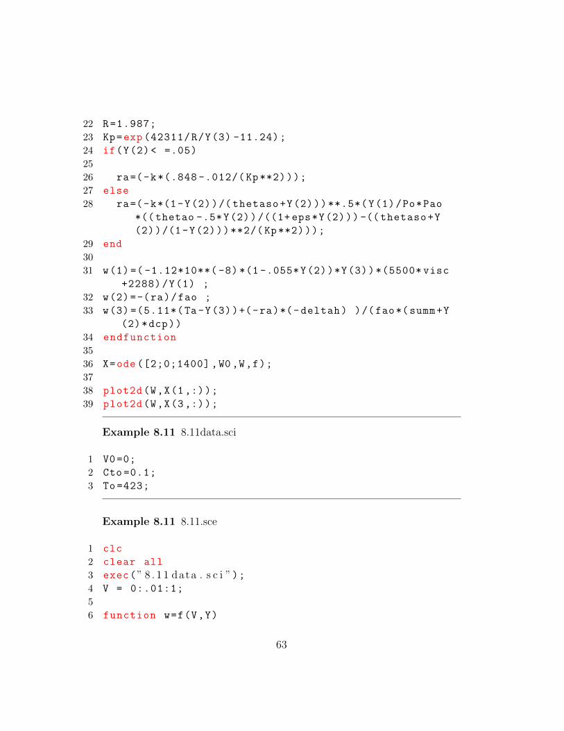
8.1 Output graph of S 8.4 . . . . . . . . . . . . . . . . . . . . . 538.2 Output graph of S 8.6 . . . . . . . . . . . . . . . . . . . . . 558.3 Output graph of S 8.6 . . . . . . . . . . . . . . . . . . . . . 568.4 Output graph of S 8.6 . . . . . . . . . . . . . . . . . . . . . 578.5 Output graph of S 8.7 . . . . . . . . . . . . . . . . . . . . . 598.6 Output graph of S 8.7 . . . . . . . . . . . . . . . . . . . . . 608.7 Output graph of S 8.8 . . . . . . . . . . . . . . . . . . . . . 628.8 Output graph of S 8.11 . . . . . . . . . . . . . . . . . . . . . 648.9 Output graph of S 8.11 . . . . . . . . . . . . . . . . . . . . . 658.10 Output graph of S 8.12 . . . . . . . . . . . . . . . . . . . . . 68
9.1 Output graph of S 9.1 . . . . . . . . . . . . . . . . . . . . . 709.2 Output graph of S 9.1 . . . . . . . . . . . . . . . . . . . . . 71
7
9.3 Output graph of S 9.2 . . . . . . . . . . . . . . . . . . . . . 739.4 Output graph of S 9.3 . . . . . . . . . . . . . . . . . . . . . 759.5 Output graph of S 9.3 . . . . . . . . . . . . . . . . . . . . . 769.6 Output graph of S 9.4 . . . . . . . . . . . . . . . . . . . . . 809.7 Output graph of S 9.4 . . . . . . . . . . . . . . . . . . . . . 819.8 Output graph of S 9.4 . . . . . . . . . . . . . . . . . . . . . 829.9 Output graph of S 9.8 . . . . . . . . . . . . . . . . . . . . . 849.10 Output graph of S 9.8 . . . . . . . . . . . . . . . . . . . . . 85
10.1 Output graph of S 10.5 . . . . . . . . . . . . . . . . . . . . . 8810.2 Output graph of S 10.5 . . . . . . . . . . . . . . . . . . . . . 8910.3 Output graph of S 10.5 . . . . . . . . . . . . . . . . . . . . . 9110.4 Output graph of S 10.7 . . . . . . . . . . . . . . . . . . . . . 93
14.1 Output graph of S 14.3 . . . . . . . . . . . . . . . . . . . . . 104
8
Chapter 1
Mole Balances
1.1 Discussion
When executing the code from the editor, use the ’Execute File into Scilab’taband not the ’Load in Scilab’tab. The .sci files of the respective problems con-tain the input parameters of the question
1.2 Scilab Code
Example 1.3 1.3data.sci
1 k = 0.23; // minˆ−12 v0 = 10; //dmˆ3/ min
Example 1.3 1.3.sce
1 clc
2 clear all
3 exec(” 1 . 3 data . s c i ”);4
5 //CA = 0 . 1∗CA0 ;6 V = (v0/k)*log (1/0.1);
7 disp(”V =”)8 disp(V)
9 disp (”dmˆ3 ”)
9

10
Chapter 2
Conversion and Reactor Sizing
2.1 Discussion
When executing the code from the editor, use the ’Execute File into Scilab’taband not the ’Load in Scilab’tab. The .sci files of the respective problems con-tain the input parameters of the question
2.2 Scilab Code
Example 2.1 2.1data.sci
1 P0 = 10; //atm2 yA0 = 0.5;
3 T0 = 422.2; //K4 R = 0.082; // dmˆ 3 . atm/mol .K5 v0 = 6; //dmˆ3/ s
Example 2.1 2.1.sce
1 clc
2 clear all
3 exec(” 2 . 1 data . s c i ”);4 CA0=(yA0*P0)/(R*T0);
5 FA0 = CA0*v0;
6 disp(”CA0 =”)
11
7 disp(CA0)
8 disp (”mol/dmˆ3 ”)9 disp(”FA0 =”)10 disp(FA0)
11 disp(”mol/ s ”)
Example 2.2 2.2data.sci
1 P0 = 10; //atm2 yA0 = 0.5;
3 T0 = 422.2; //K4 R = 0.082; // dmˆ 3 . atm/mol .K5 v0 = 6; //dmˆ3/ s6 X = 0.8;
7 rA = -1/800; //1/−rA = 800//dmˆ 3 . s /mol
Example 2.2 2.2.sce
1 clc
2 clear all
3 exec(” 2 . 2 data . s c i ”);4 CA0=(yA0*P0)/(R*T0);
5 FA0 = CA0*v0;
6 V = FA0*X*(1/-rA)
7
8 disp(”FA0 =”)9 disp(FA0)
10 disp(”mol/ s ”)11 disp(”V =”)12 disp(V)
13 disp (”dmˆ3 ”)
Example 2.3 2.3data.sci
1 P0 = 10; //atm2 yA0 = 0.5;
3 T0 = 422.2; //K
12
4 R = 0.082; // dmˆ 3 . atm/mol .K5 v0 = 6; //dmˆ3/ s6 X = [0 0.1 0.2 0.3 0.4 0.5 0.6 0.7 0.8]’;
7 p = [189 192 200 222 250 303 400 556 800]; //1/−rA =800//dmˆ 3 . s / mols
Example 2.3 2.3.sce
1 clc
2 clear all
3 exec(” 2 . 3 data . s c i ”);4 CA0=(yA0*P0)/(R*T0);
5 FA0 = CA0*v0;
6 //V = FA0∗X∗(1/−rA )7
8 V = FA0*inttrap(X,p)
9 disp(”FA0 =”)10 disp(FA0)
11 disp(”mol/ s ”)12 disp(”V =”)13 disp(V)
14 disp (”dmˆ3 ”)15 disp(” Answer i s s l i g h t l y d i f f e r e n n t from the book
because i n t t r a p command o f SCILAB u s e st r a p e z o i d a l i n t e g r a t i o n , w h i l e i n book i t hasbeen c a l c u l a t e d u s i n g f i v e p o i n t f o rmu la e . ”)
Example 2.4 2.4data.sci
1 FA0 = 5; // mol/ s2 rAat = -(1/400);
3
4 X = [0 0.1 0.2 0.3 0.4 0.5 0.6]’;
5 p = [189 192 200 222 250 303 400]; //1/−rA = 800//dmˆ 3 . s / mols
Example 2.4 2.4.sce
13
1 clc
2 clear all
3 exec(” 2 . 4 data . s c i ”);4
5
6 VCSTR = FA0*X(7)*(1/- rAat);
7 VPFR = FA0*inttrap(X,p)
8 disp(”VCSTR =”)9 disp(VCSTR)
10 disp(”dmˆ3 ”)11 disp(”VPFR =”)12 disp(VPFR)
13 disp (”dmˆ3 ”)
Example 2.5 2.5data.sci
1 FA0 = 0.867; // mol/ s2 rA = -(1/250);
3 rA2 = -(1/800);
4 X = 0.8;
5 X1 = 0.4;
6 X2 = 0.8
Example 2.5 2.5.sce
1 clc
2 clear all
3 exec(” 2 . 5 data . s c i ”);4
5
6 V1 = FA0*X1*(1/-rA);
7 V2 = FA0*(X2-X1)*(1/-rA2);
8 V = FA0*X*(1/-rA2);
9 disp(”V1 =”)10 disp(V1)
11 disp(”dmˆ3 ”)12 disp(”V2 =”)13 disp(V2)
14
14 disp (”dmˆ3 ”)15 disp(”V =”)16 disp(V)
17 disp (”dmˆ3 ”)
Example 2.6 2.6data.sci
1 FA0 = 0.867; // mol/ s2 X = [0 0.1 0.2 0.3 0.4 0.5 0.6 0.7 0.8]’;
3 p = [189 192 200 222 250 303 400 556 800]; //1/−rA =800//dmˆ 3 . s / mols
Example 2.6 2.6.sce
1 clc
2 clear all
3 exec(” 2 . 6 data . s c i ”);4
5
6 X1 = X(1:5);
7 p1 = p(1:5);
8 V1 = FA0*inttrap(X1,p1)
9 X2 = X(5:9);
10 p2 = p(5:9);
11 V2 = FA0*inttrap(X2,p2)
12 V=V1+V2;
13 disp(”V1 =”)14 disp(V1)
15 disp(”dmˆ3 ”)16 disp(”V2 =”)17 disp(V2)
18 disp (”dmˆ3 ”)19 disp(”V =”)20 disp(V)
21 disp (”dmˆ3 ”)
Example 2.7 2.7data.sci
15
1 FA0 = 0.867; // mol/ s2 X1 = 0.5;
3 X2 = 0.8;
4 rA2 = -(1/800);
5 X = [0 0.1 0.2 0.3 0.4 0.5 0.6 0.7 0.8]’;
6 p = [189 192 200 222 250 303 400 556 800]; //1/−rA =800//dmˆ 3 . s / mols
Example 2.7 2.7.sce
1 clc
2 clear all
3 exec(” 2 . 7 data . s c i ”);4
5
6 X = X(1:6);
7 p = p(1:6);
8 V1 = FA0*inttrap(X,p);
9 V2 = FA0*(X2 -X1)*(1/-rA2);
10 V=V1+V2;
11 disp(”V1 =”)12 disp(V1)
13 disp(”dmˆ3 ”)14 disp(”V2 =”)15 disp(V2)
16 disp (”dmˆ3 ”)17 disp(”V =”)18 disp(V)
19 disp (”dmˆ3 ”)
16
Chapter 3
Rate Laws and Stoichiometry
3.1 Discussion
When executing the code from the editor, use the ’Execute File into Scilab’taband not the ’Load in Scilab’tab. The .sci files of the respective problems con-tain the input parameters of the question
3.2 Scilab Code
Example 3.5 3.5data.sci
1 CA0 = 10;
2 CB0 = 2;
3 X = 0.2;
4 X1=0.9
Example 3.5 3.5.sce
1 clc
2 clear all
3 exec(” 3 . 5 data . s c i ”);4 CD=CA0*(X/3);
5 CB=CA0*(( CB0/CA0) -(X/3));
6 CD1=CA0*(X1/3);
7 CB1=CA0*((CB0/CA0)-(X1/3));
17
8 disp(” For 20% c o n v e r s i o n ”)9 disp(”CD =”)10 disp(CD)
11 disp (”mol/dmˆ3 ”)12 disp(”CB =”)13 disp(CB)
14 disp(”mol/dmˆ3 ”)15 disp(” For 90% c o n v e r s i o n ”)16 disp(”CD =”)17 disp(CD1)
18 disp (”mol/dmˆ3 ”)19 disp(”CB =”)20 disp(CB1)
21 disp(”mol/dmˆ3 ”)
18
Chapter 4
Isothermal Reactor Design
4.1 Discussion
When executing the code from the editor, use the ’Execute File into Scilab’taband not the ’Load in Scilab’tab. The .sci files of the respective problems con-tain the input parameters of the question
4.2 Scilab Code
Example 4.1 4.1data.sci
1 t = [0 0.5 1 1.5 2 3 4 6 10];
2 CC = [0 0.145 .27 .376 .467 .61 .715 .848 .957];
3 CA0 = 1;
Example 4.1 4.1.sce
1 clc
2 clear all
3 exec(” 4 . 1 data . s c i ”);4
5 x=t;
6 y =((CA0 -CC)/CA0);
7
8 yi=interpln ([x;y],x);
19
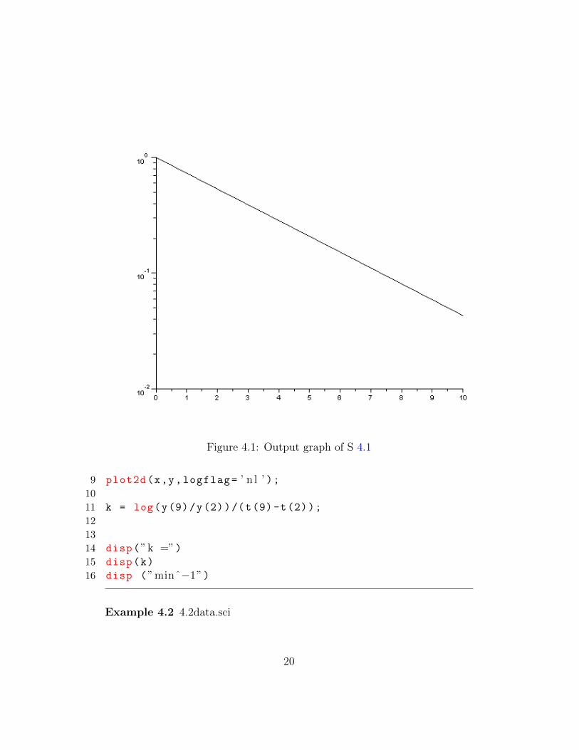
Figure 4.1: Output graph of S 4.1
9 plot2d(x,y,logflag= ’ n l ’ );10
11 k = log(y(9)/y(2))/(t(9)-t(2));
12
13
14 disp(”k =”)15 disp(k)
16 disp (”minˆ−1”)
Example 4.2 4.2data.sci
20
1 k = 0.311; // minˆ−1;2 FC= 6.137; // l b . mol/min3 X = 0.8;
4 CA01= 1; // mol/dmˆ3
Example 4.2 4.2.sce
1 clc
2 clear all
3 exec(” 4 . 2 data . s c i ”);4
5 FA0 = FC/X;
6 vA0 = FA0/CA01;
7 vB0 = vA0;
8 v0 = vA0+vB0;
9 V = v0*X/(k*(1-X));
10
11 // CSTR i n p a r a l l e l12 V1 = 800/7.48;
13
14 Tau =V1/(v0/2);
15 Da= Tau*k;
16 Xparallel = Da/(1+Da)
17
18 // CSTR i n s e r i e s19 Tau =V1/v0;
20 n=2;
21 Xseries = 1- (1/(1+ Tau*k)^n);
22
23 disp(” Reactor volume ”)24 disp(V)
25 disp (” f t ˆ3 ”)26 disp(”CSTR i n p a r a l l e l X =”)27 disp(Xparallel)
28 disp(”CSTR i n s e r i e s X =”)29 disp(Xseries)
Example 4.4 4.4data.sci
21
1 k1 = 0.072; // s ˆ−1;2 yA0 = 1;
3 P0= 6; //atm4 R = 0.73; // atm/ l b . mol . oR5 T0 = 1980; //oR6 T1 = 1000; //K7 T2 = 1100; // K8 e=1;
9 E = 82000; // c a l /g . mol10 FB= 0.34; // l b . mol/ s11 X = 0.8;
Example 4.4 4.4.sce
1 clc
2 clear all
3 exec(” 4 . 4 data . s c i ”);4
5 FA0 = FB/X;
6 CA0 = yA0*P0/(R*T0);
7 R = 1.987;
8 k2 = k1*exp((E/R)*((1/T1) -(1/T2)));
9 V =( FA0/(k2*CA0))*((1+e)*log(1/(1-X))-e*X);
10
11 disp(” Reactor volume ”)12 disp(V)
13 disp(” f t ˆ3 ”)
Example 4.5 4.5data.sci
1 Ac = 0.01414; // f t ˆ22 m = 104.4; // lbm/h3 mu = 0.0673; // lbm/ f t . h4 Dp = 0.0208; // f t5 gc = 4.17e8; // lbm . f t / l b f . hˆ26 phi = 0.45;
7 rho = 0.413; // lbm/ f t ˆ38 P0 = 10; // atm
22
9 L = 60; // f t
Example 4.5 4.5.sce
1 clc
2 clear all
3 exec(” 4 . 5 data . s c i ”);4
5 G = m/Ac;
6 bita0 = (G*(1-phi)/(gc*rho*Dp*phi^3))*((150*(1 - phi)*
mu/Dp)+1.75*G);
7 bita0 = bita0 /(144*14.7);//atm/ f t8 P = ((1 -(2* bita0*L/P0))^.5)*P0;
9 deltaP = P0 - P;
10
11 disp(” de l t aP ”)12 disp(deltaP)
13 disp(”atm”)
Example 4.6 4.6data.sci
1 k = 0.0141; // l b . mol/atm . l b ca t . h2 FA0 = 1.08; // l b . mol/h3 FB0 = 0.54; // l b . mol/h4 FI = 2.03; // l b . mol/h5 bita0 = 0.0775; // atm/ f t6 Ac = 0.01414; // f t ˆ27 phi = 0.45;
8 rhoc = 120; // l b c a t / f t ˆ39 P0 = 10; // atm
10 X = 0.6;
Example 4.6 4.6.sce
1 clc
2 clear all
3 exec(” 4 . 6 data . s c i ”);
23
4
5 FT0 = FA0+FB0+FI;
6 yA0 = FA0/FT0;
7 e = yA0*(1-.5 -1);
8 PA0 = yA0*P0;
9 kdes = k*PA0 *(1/2) ^(2/3);
10 alpha = 2*bita0 /(Ac*(1-phi)*rhoc*P0);
11 W = (1 - (1 -(3* alpha*FA0 /(2* kdes))*((1+e)*log(1/(1-X
))-e*X))^(2/3))/alpha;
12
13
14 disp(”W”)15 disp(W)
16 disp(” l b o f c a t a l y s t per tube ”)
Example 4.7 4.7data.sci
1 kprime = 0.0266; // l b . mol/atm . l b ca t . h2 alpha = 0.0166;
3 e = -0.15;
4 W0 = 0;
5 FA0 =1;
Example 4.7 4.7.sce
1 clc
2 clear all
3 exec(” 4 . 7 data . s c i ”);4 W = 0:1:60;
5 function w=f(W,Y)
6
7 w=zeros (2,1);
8 w(1)= (kprime/FA0)*((1-Y(1))/(1+e*Y(1)))*Y(2);
9 w(2) = -alpha *(1+e*Y(1))/(2*Y(2));
10 endfunction
11
12
13 x=ode ([0;1] ,W0 ,W,f);
24
14 for i= 1:61
15 F(i) = (1+e*x(1,i))/x(2,i);
16 end
17 F= F’;
18 for i= 1:61
19 rate(i) = (kprime)*((1-x(1,i))/(1+e*x(1,i)))*x(2,i
);
20 end
21 rate =rate ’;
22
23 scf (1)
24 plot2d(W,rate);
25 xtitle( ’ F i gu r e E4−7.1 Reac t i on r a t e p o r f i l e downthe PBR ’ , ’w ’ , ’ r a t e ’ ) ;
26 scf (2)
27
28 l1=x(1,: )’
29 l2=x(2,: )’
30 l3=F’
31 plot2d(W’,[l1 l2 l3]);
32
33 xtitle( ’ F i gu r e E4−7.2 ’ , ’w ’ , ’ x , y , z ’ ) ;
34 legend ([ ’ x ’ ; ’ y ’ ; ’ f ’ ]);
Example 4.8 4.8data.sci
1 FA0 = 440;
2 P0 = 2000;
3 Ca0 = .32;
4 R = 30;
5 phi = .4;
6 kprime = 0.02; // l b . mol/atm . l b ca t . h7 L = 27;
8 rhocat = 2.6;
9 m=44;
10
11 alpha = 0.0166;
25
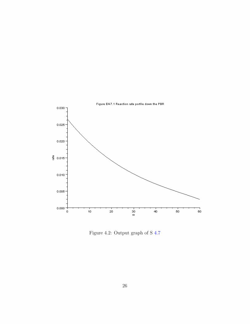
Figure 4.2: Output graph of S 4.7
26
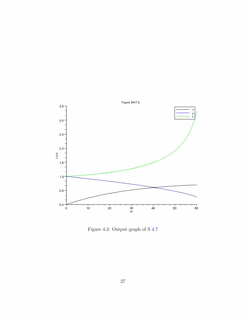
Figure 4.3: Output graph of S 4.7
27
12 e = -0.15;
13 Z0 = 0;
Example 4.8 4.8.sce
1 clc
2 clear all
3 exec(” 4 . 8 data . s c i ”);4 Z = 0:1:12;
5 function w=f(Z,Y)
6
7 w=zeros (2,1);
8 Ac= 3.14*((R^2) -(Z-L)^2);
9 Ca = Ca0*(1-Y(1))*Y(2) /(1+Y(1));
10 ra =kprime*Ca*rhocat *(1-phi);
11 G= m/Ac;
12 V =3.14*(Z*(R^2) -(1.3*(Z-L)^3) -(1/3)*L^3)
13 bita = (98.87*G+25630*G^2) *0.01;
14 W=rhocat *(1-phi)*V
15 w(1)= -ra*Ac/FA0
16 w(2) = -bita/P0/(Y(2) *(1+Y(1)));
17 endfunction
18
19
20 x=ode ([0;1] ,Z0 ,Z,f);
21 for i= 1: length(Z)
22 V(1,i) =3.14*Z(1,i)*((R^2) -(Z(1,i)-L)^2)
23 W1(1,i)=rhocat *(1-phi)*V(1,i)
24 end
25
26 l1=x(1,: )’
27 l2=x(2,: )’
28
29 plot2d(W1 ’,[l1 l2]);
30
31 xtitle( ’ F i gu r e E4−8.2 ’ , ’w ’ , ’ x , y ’ ) ;
32 legend ([ ’ x ’ ; ’ y ’ ]);
28
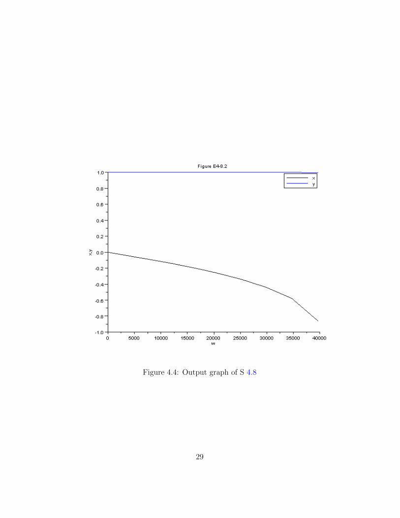
Figure 4.4: Output graph of S 4.8
29
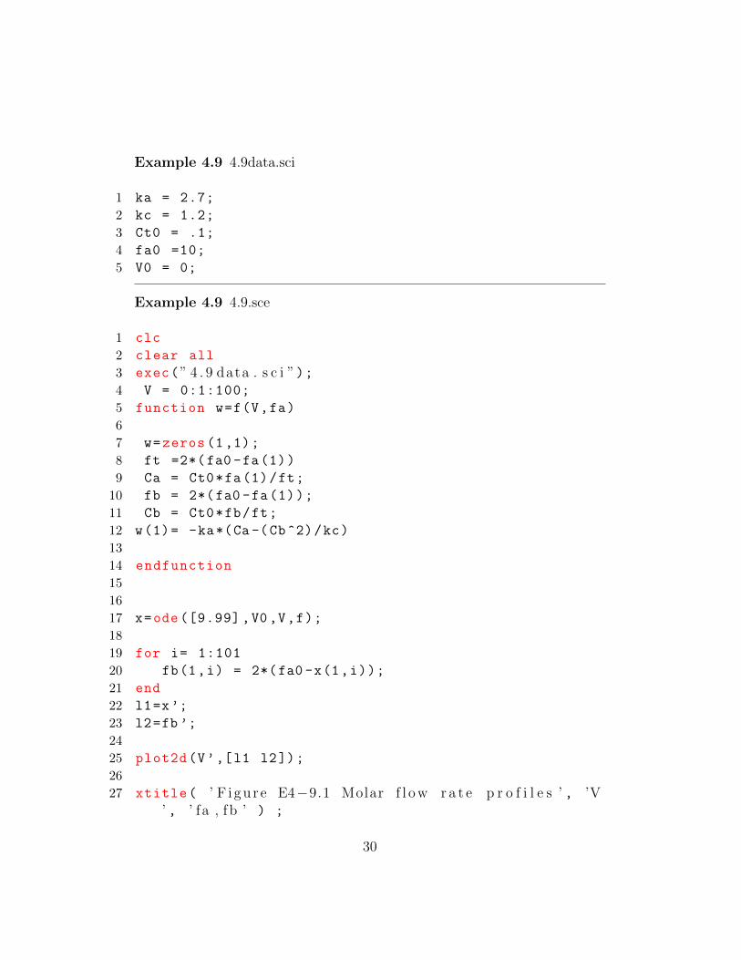
Example 4.9 4.9data.sci
1 ka = 2.7;
2 kc = 1.2;
3 Ct0 = .1;
4 fa0 =10;
5 V0 = 0;
Example 4.9 4.9.sce
1 clc
2 clear all
3 exec(” 4 . 9 data . s c i ”);4 V = 0:1:100;
5 function w=f(V,fa)
6
7 w=zeros (1,1);
8 ft =2*(fa0 -fa(1))
9 Ca = Ct0*fa(1)/ft;
10 fb = 2*(fa0 -fa(1));
11 Cb = Ct0*fb/ft;
12 w(1)= -ka*(Ca -(Cb^2)/kc)
13
14 endfunction
15
16
17 x=ode ([9.99] ,V0 ,V,f);
18
19 for i= 1:101
20 fb(1,i) = 2*(fa0 -x(1,i));
21 end
22 l1=x’;
23 l2=fb ’;
24
25 plot2d(V’,[l1 l2]);
26
27 xtitle( ’ F i gu r e E4−9.1 Molar f l o w r a t e p r o f i l e s ’ , ’V’ , ’ fa , f b ’ ) ;
30
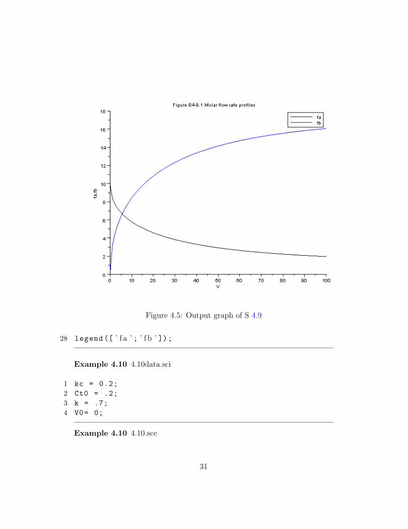
Figure 4.5: Output graph of S 4.9
28 legend ([ ’ f a ’ ; ’ f b ’ ]);
Example 4.10 4.10data.sci
1 kc = 0.2;
2 Ct0 = .2;
3 k = .7;
4 V0= 0;
Example 4.10 4.10.sce
31
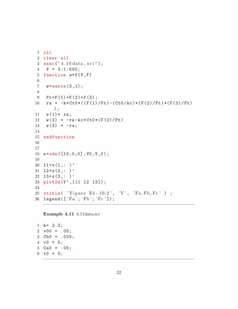
1 clc
2 clear all
3 exec(” 4 . 1 0 data . s c i ”);4 V = 0:1:500;
5 function w=f(V,F)
6
7 w=zeros (3,1);
8
9 Ft=F(1)+F(2)+F(3);
10 ra = -k*Ct0 *((F(1)/Ft)-(Ct0/kc)*(F(2)/Ft)*(F(3)/Ft)
);
11 w(1)= ra;
12 w(2) = -ra-kc*Ct0*(F(2)/Ft)
13 w(3) = -ra;
14
15 endfunction
16
17
18 x=ode ([10;0;0] ,V0,V,f);
19
20 l1=x(1,: )’
21 l2=x(2,: )’
22 l3=x(3,: )’
23 plot2d(V’,[l1 l2 l3]);
24
25 xtitle( ’ F i gu r e E4−10.2 ’ , ’V ’ , ’ Fa , Fb , Fc ’ ) ;
26 legend ([ ’ Fa ’ ; ’Fb ’ ; ’ Fc ’ ]);
Example 4.11 4.11data.sci
1 k= 2.2;
2 v00 = .05;
3 Cb0 = .025;
4 v0 = 5;
5 Ca0 = .05;
6 t0 = 0;
32
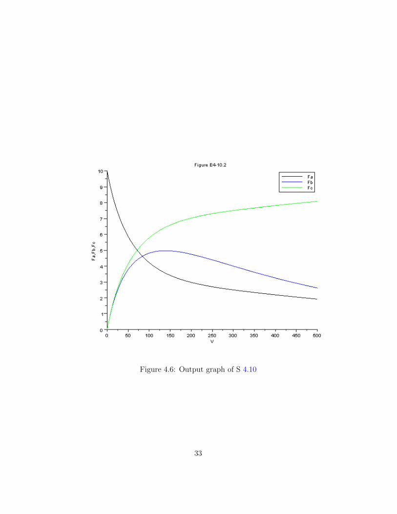
Figure 4.6: Output graph of S 4.10
33
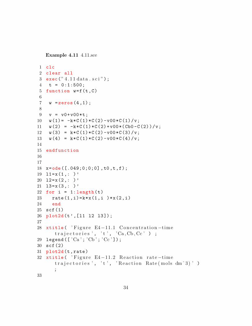
Example 4.11 4.11.sce
1 clc
2 clear all
3 exec(” 4 . 1 1 data . s c i ”);4 t = 0:1:500;
5 function w=f(t,C)
6
7 w =zeros (4,1);
8
9 v = v0+v00*t;
10 w(1)= -k*C(1)*C(2)-v00*C(1)/v;
11 w(2) = -k*C(1)*C(2)+v00*(Cb0 -C(2))/v;
12 w(3) = k*C(1)*C(2)-v00*C(3)/v;
13 w(4) = k*C(1)*C(2)-v00*C(4)/v;
14
15 endfunction
16
17
18 x=ode ([.049;0;0;0] ,t0,t,f);
19 l1=x(1,: )’
20 l2=x(2,: )’
21 l3=x(3,: )’
22 for i = 1: length(t)
23 rate(1,i)=k*x(1,i )*x(2,i)
24 end
25 scf (1)
26 plot2d(t’,[l1 l2 l3]);
27
28 xtitle( ’ F i gu r e E4−11.1 Concent ra t i on−t imet r a j e c t o r i e s ’ , ’ t ’ , ’Ca , Cb , Cc ’ ) ;
29 legend ([ ’Ca ’ ; ’Cb ’ ; ’ Cc ’ ]);30 scf (2)
31 plot2d(t,rate)
32 xtitle( ’ F i gu r e E4−11.2 Reac t i on ra t e−t imet r a j e c t o r i e s ’ , ’ t ’ , ’ Reac t i on Rate ( mols dmˆ3) ’ )
;
33
34
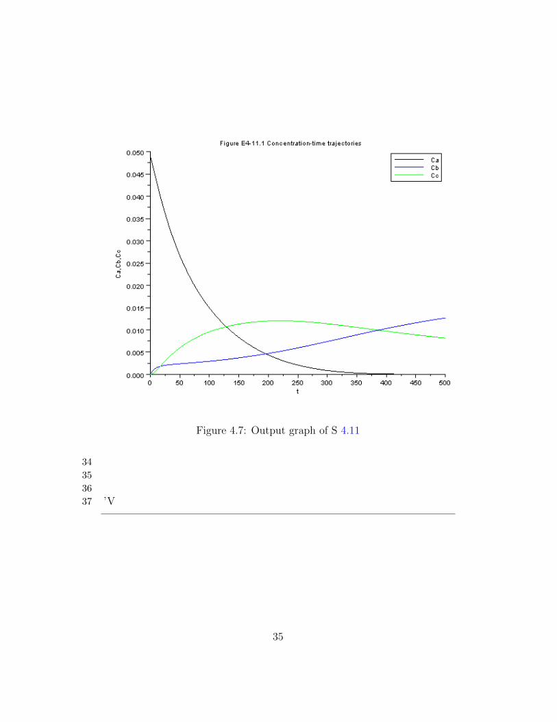
Figure 4.7: Output graph of S 4.11
34
35
36
37 ’V
35
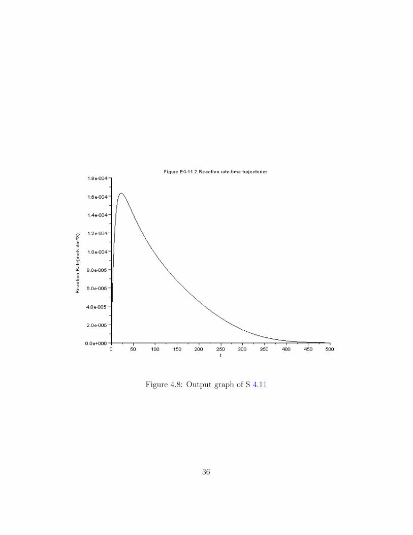
Figure 4.8: Output graph of S 4.11
36
Chapter 5
Collection and Analysis of RateData
5.1 Discussion
When executing the code from the editor, use the ’Execute File into Scilab’taband not the ’Load in Scilab’tab. The .sci files of the respective problems con-tain the input parameters of the question
5.2 Scilab Code
Example 5.2 5.2data.sci
1 t = [0 2.5 5 10 15 20]’;
2 P = [7.5 10.5 12.5 15.8 17.9 19.4] ’;
3 P0 = 7.5;
Example 5.2 5.2.sce
1 clc
2 clear all
3 exec(” 5 . 2 data . s c i ”);4 for i =1: length(t)
5 g(i) =log (2*P0/(3*P0 -P(i)));
6 end
37
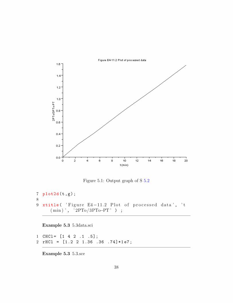
Figure 5.1: Output graph of S 5.2
7 plot2d(t,g);
8
9 xtitle( ’ F i gu r e E4−11.2 P lo t o f p r o c e s s e d data ’ , ’ t( min ) ’ , ’ 2PTo/3PTo−PT ’ ) ;
Example 5.3 5.3data.sci
1 CHCl= [1 4 2 .1 .5];
2 rHCl = [1.2 2 1.36 .36 .74]*1 e7;
Example 5.3 5.3.sce
38
1 clc
2 clear all
3 exec(” 5 . 3 data . s c i ”);4
5 x=log(CHCl);
6 y=log(-rHCl);
7 plot2d(x,y);
8
9 xtitle( ’ F i gu r e E5−3.2 ’ , ’CHCl ( g mol/ l i t e r ) ’ , ’rHCl0 ( g mol / cm ˆ 2 . s ) ’ ) ;
Example 5.4 5.4data.sci
1 CCH4 = [2.44 4.44 10 1.65 2.47 1.75] ’*1e-4;
2 PCO= [1 1.8 4.08 1 1 1]’;
3 v0 =300;
4 W= 10;
Example 5.4 5.4.sce
1 clc
2 clear all
3 exec(” 5 . 4 data . s c i ”);4
5 rCH4 = (v0/W)*CCH4;x
6 x=log(PCO);
7 y = log(rCH4)
8 alpha= (y(3)-y(2))/(x(3)-x(2));
9 // p l o t 2 d ( x , y )10 disp(” a lpha ”)11 disp(alpha)
39
Chapter 6
Multiple Reactions
6.1 Discussion
When executing the code from the editor, use the ’Execute File into Scilab’taband not the ’Load in Scilab’tab. The .sci files of the respective problems con-tain the input parameters of the question
6.2 Scilab Code
Example 6.6 6.6data.sci
1 k1= 55.2;
2 k2 =30.2;
3 t0=0;
Example 6.6 6.6.sce
1 clc
2 clear all
3 exec(” 6 . 6 data . s c i ”);4 t = 0:.01:.5;
5 function w=f(t,c)
6
7 w =zeros (3,1);
8
40
9 r1 = -k1*c(2)*c(1) ^.5;
10 r2 = -k2*c(3)*c(1) ^.5;
11 w(1)= r1+r2;
12 w(2) = r1;
13 w(3) = -r1+r2;
14
15 endfunction
16
17 x=ode ([.021;.0105;0] ,t0 ,t,f);
18
19 l1=x(1,: )’
20 l2=x(2,: )’
21 l3=x(3,: )’
22
23 plot2d(t’,[l1 l2 l3]);
24
25 xtitle( ’ F i gu r e E6−6.1 ’ , ’ Tau ( hr ) ’ , ’ C o n c e n t r a t i o n( l b mol/ f t ˆ3 ’ ) ;
26 legend ([ ’CH ’ ; ’CM’ ; ’CX ’ ]);
Example 6.8 6.8data.sci
1 v0 =0;
Example 6.8 6.8.sce
1 clc
2 clear all
3 exec(” 6 . 8 data . s c i ”);4 v = 0:.1:10;
5 function w =FF(v,f)
6
7 w =zeros (6,1);
8 ft = f(1)+f(2)+f(2)+f(4)+f(5)+f(6);
9 r1a = -5*8*(f(1)/ft)*(f(2)/ft)^2;
10 r2a = -2*4*(f(1)/ft)*(f(2)/ft);
11 r4c = -5*3.175*(f(3)/ft)*(f(1)/ft)^(2/3);
41
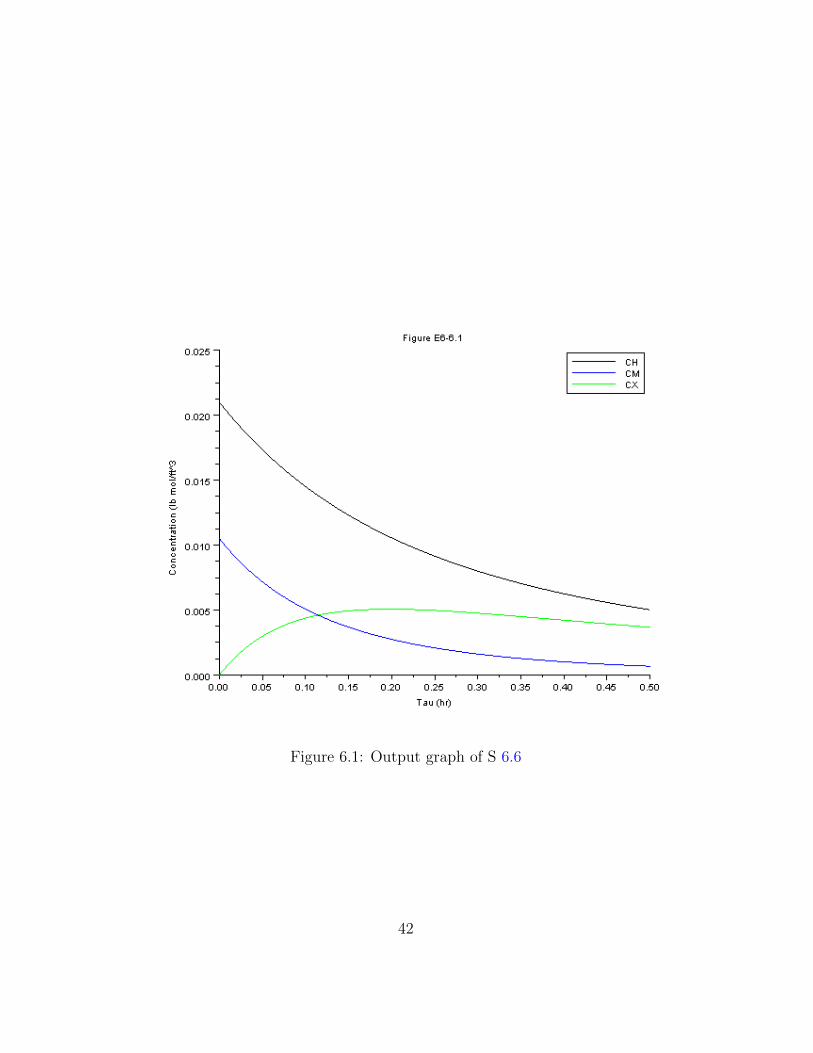
Figure 6.1: Output graph of S 6.6
42
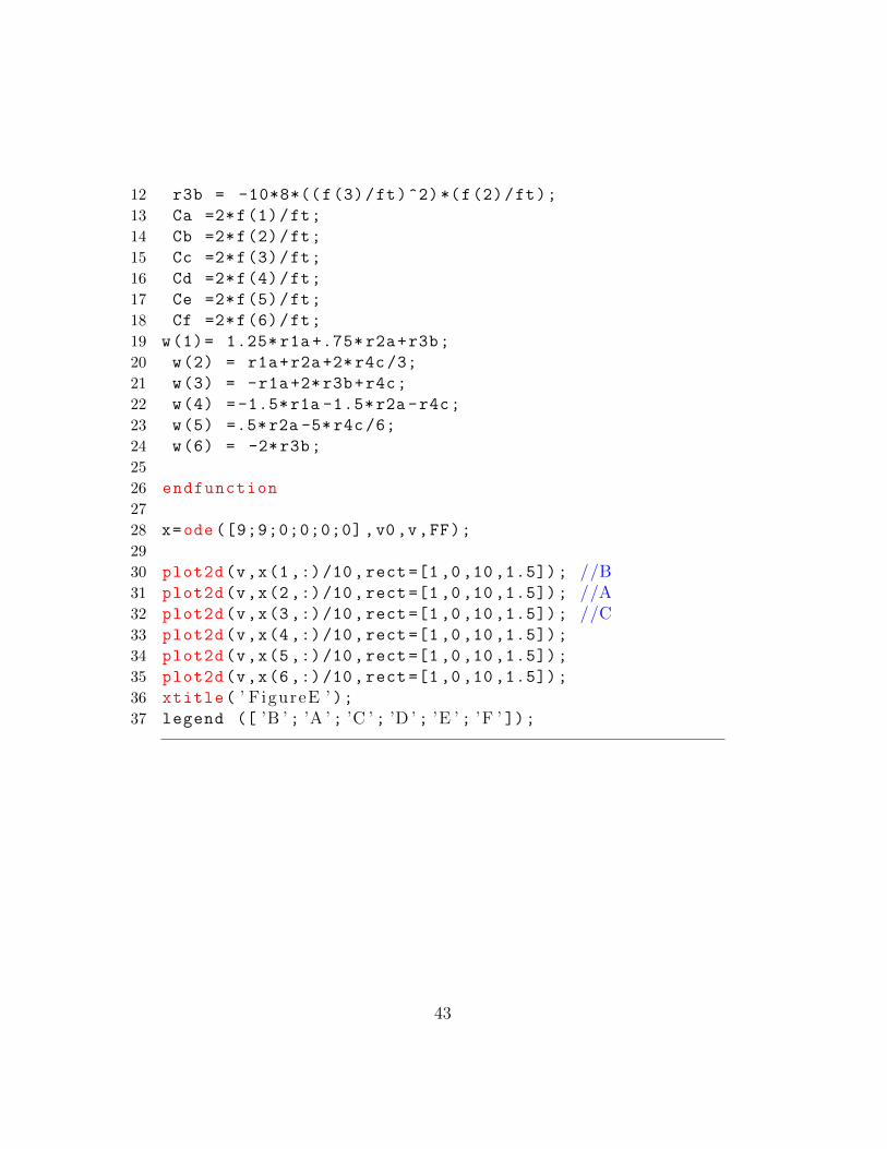
12 r3b = -10*8*((f(3)/ft)^2)*(f(2)/ft);
13 Ca =2*f(1)/ft;
14 Cb =2*f(2)/ft;
15 Cc =2*f(3)/ft;
16 Cd =2*f(4)/ft;
17 Ce =2*f(5)/ft;
18 Cf =2*f(6)/ft;
19 w(1)= 1.25* r1a +.75* r2a+r3b;
20 w(2) = r1a+r2a +2*r4c/3;
21 w(3) = -r1a+2* r3b+r4c;
22 w(4) =-1.5*r1a -1.5*r2a -r4c;
23 w(5) =.5*r2a -5*r4c /6;
24 w(6) = -2*r3b;
25
26 endfunction
27
28 x=ode ([9;9;0;0;0;0] ,v0,v,FF);
29
30 plot2d(v,x(1,:)/10,rect =[1 ,0 ,10 ,1.5]); //B31 plot2d(v,x(2,:)/10,rect =[1 ,0 ,10 ,1.5]); //A32 plot2d(v,x(3,:)/10,rect =[1 ,0 ,10 ,1.5]); //C33 plot2d(v,x(4,:)/10,rect =[1 ,0 ,10 ,1.5]);
34 plot2d(v,x(5,:)/10,rect =[1 ,0 ,10 ,1.5]);
35 plot2d(v,x(6,:)/10,rect =[1 ,0 ,10 ,1.5]);
36 xtitle( ’ F igureE ’ );37 legend ([ ’B ’ ; ’A ’ ; ’C ’ ; ’D ’ ; ’E ’ ; ’F ’ ]);
43
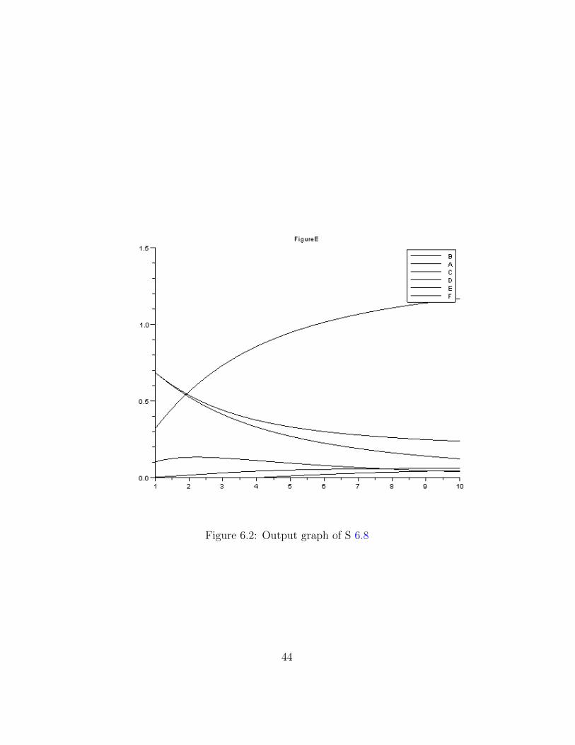
Figure 6.2: Output graph of S 6.8
44
Chapter 7
Nonelementary ReactionKinetics
7.1 Discussion
When executing the code from the editor, use the ’Execute File into Scilab’taband not the ’Load in Scilab’tab. The .sci files of the respective problems con-tain the input parameters of the question
7.2 Scilab Code
Example 7.7 7.7data.sci
1 Curea = [.2 .02 .01 .005 .002] ’;
2 rurea = -[1.08 .55 .38 .2 .09]’;
Example 7.7 7.7.sce
1 clc
2 clear all
3 exec(” 7 . 7 data . s c i ”);4 for i=1: length(Curea)
5 x(i)= 1/Curea(i);
6 y(i) = 1/(-rurea(i));
7 end
45
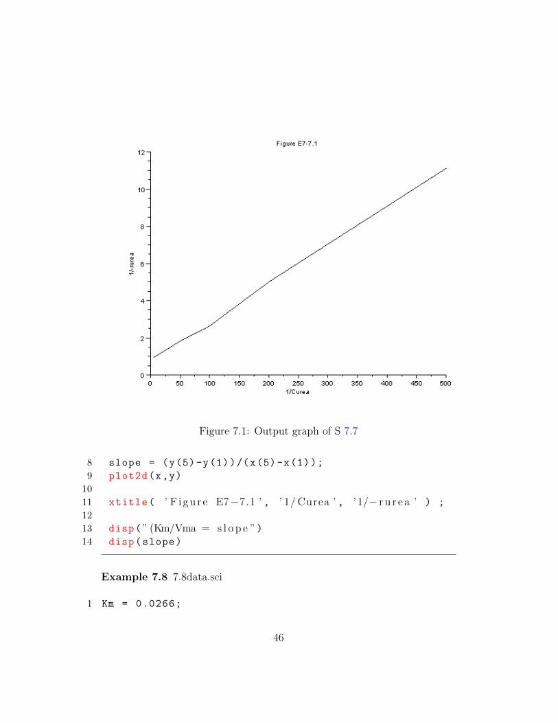
Figure 7.1: Output graph of S 7.7
8 slope = (y(5)-y(1))/(x(5)-x(1));
9 plot2d(x,y)
10
11 xtitle( ’ F i gu r e E7−7.1 ’ , ’ 1/ Curea ’ , ’ 1/− r u r e a ’ ) ;
12
13 disp(” (Km/Vma = s l o p e ”)14 disp(slope)
Example 7.8 7.8data.sci
1 Km = 0.0266;
46
2 Vmax1 = 1.33;
3 Et2 = 0.001;
4 Et1 = 5;
5 X = .8;
6 Curea0 = .1;
Example 7.8 7.8.sce
1 clc
2 clear all
3 exec(” 7 . 8 data . s c i ”);4 Vmax = (Et2/Et1)*Vmax1
5 t = (Km/Vmax)*log(1/(1-X))+Curea0*X/Vmax;
6 disp(” t ”)7 disp(t)
8 disp(” s ”)
Example 7.9 7.9data.sci
1 ysc =1/.08;
2 ypc = 5.6;
3 ks = 1.7;
4 m = 0.03;
5 umax = .33;
6 t0 = 0;
Example 7.9 7.9.sce
1 clc
2 clear all
3 exec(” 7 . 9 data . s c i ”);4 t = 0:.1:12;
5 function w=f(t,c)
6
7 w =zeros (3,1);
8
9 rd = c(1) *.01;
47
10 rsm = m/c(1);
11 kobs= (umax*(1-c(3) /93) ^.52);
12 rg= kobs*c(1)*c(2)/(ks+c(2));
13 // r2 = −k2∗ c ( 3 ) ∗ c ( 1 ) ˆ . 5 ;14 w(1)= rg -rd;
15 w(2) = ysc*(-rg)-rsm;
16 w(3) = rg*ypc;
17
18 endfunction
19
20 x=ode ([1;250;0] ,t0,t,f);
21
22 l1=x(1,: )’
23 l2=x(2,: )’
24 l3=x(3,: )’
25
26 plot2d(t’,[l1 l2 l3]);
27
28 xtitle( ’ F i gu r e E7−9.1 c o n c e n t r a t i o n s as a f u n c t i o no f t ime ’ , ’ t ( hr ) ’ , ’C ( g/dmˆ3) ’ ) ;
29 legend ([ ’ Cc ’ ; ’ Cs ’ ; ’Cp ’ ]);
48
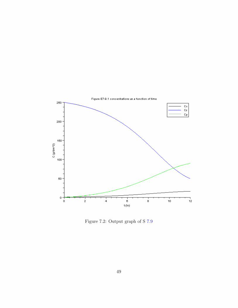
Figure 7.2: Output graph of S 7.9
49
Chapter 8
Steady State NonisothermalReactor Design
8.1 Discussion
When executing the code from the editor, use the ’Execute File into Scilab’taband not the ’Load in Scilab’tab. The .sci files of the respective problems con-tain the input parameters of the question
8.2 Scilab Code
Example 8.3 8.3data.sci
1 H0NH3 = -11020; // c a l /moleN22 H0H2 = 0;
3 HN2 = 0;
4 CpNH3 = 8.92; // c a l /moleH2 .K5 CpH2 = 6.992; // c a l /moleN2 .K6 CpN2 =6.984; // c a l /moleNH3 .K7 T = 423; //K8 TR = 298; //K
Example 8.3 8.3.sce
1 clc
50
2 clear all
3 exec(” 8 . 3 data . s c i ”);4 deltaHRx0 = 2*H0NH3 -3*H0H2 -HN2;
5 deltaCp = 2*CpNH3 -3*CpH2 -CpN2;
6 deltaHRx = deltaHRx0+deltaCp *(T-TR);
7 disp(”The heat o f r e a c t i o n on the b a s i s on the moleso f H2 r e a c t e d i s =”)
8 disp ((1/3)*deltaHRx *4.184)
9 disp(”J at 423 K”)
Example 8.4 8.4data.sci
1 T =[535 550 565 575 585 595 605 615 625] ’;
2 H0C= -226000;
3 H0B = -123000;
4 H0A = -66600;
5 CpC = 46;
6 CpB = 18;
7 CpA = 35;
8 CpM = 19.5;
9 TR = 528;
10 Ti0 = 535;
11 vA0 = 46.62;
12 vB0 = 46.62;
13 VM0 = 233.1;
14 V = 40.1;
15 FA0 =43.04;
16 FM0 = 71.87;;
17 FB0 = 802.8;
18 A = 16.96 e12;
19 E = 32400;
20 R = 1.987;
Example 8.4 8.4.sce
1 clc
2 clear all
3 exec(” 8 . 4 data . s c i ”);
51
4 HRx0 = H0C -H0B -H0A;
5 deltaCp = CpC -CpB -CpA;
6 deltaHRx0 = HRx0+deltaCp *(TR-TR);
7 v0 = vA0+vB0+VM0;
8 tau = V/v0;
9 CA0 = FA0/v0;
10 phiM0 = FM0/FA0;
11 phiB0 = FB0/FA0;
12 Cpi = CpA+phiB0*CpB+phiM0*CpM;
13
14 for i =1: length(T)
15 XEB(i) = -Cpi*(T(i)-Ti0)/( deltaHRx0+deltaCp *(T(i)-TR
));
16 XMB(i) = tau*A*exp(-E/(R*T(i)))/(1+ tau*A*exp(-E/(R*T
(i))));
17 end
18
19
20
21 plot2d(T’,[XEB XMB]);
22
23 xtitle( ’ F i gu r e E8−4.2 ’ , ’T(oR) ’ , ’ Convers ion , X ’ )
;
24 legend ([ ’XEB ’ ; ’XMB’ ]);
Example 8.6 8.6data.sci
1 Fa0 = .9*163;
2 Ca0 = 9.3;
3 V0 = 0;
Example 8.6 8.6.sce
1 clc
2 clear all
3 exec(” 8 . 6 data . s c i ”);4 V = 0:.1:3.6;
52
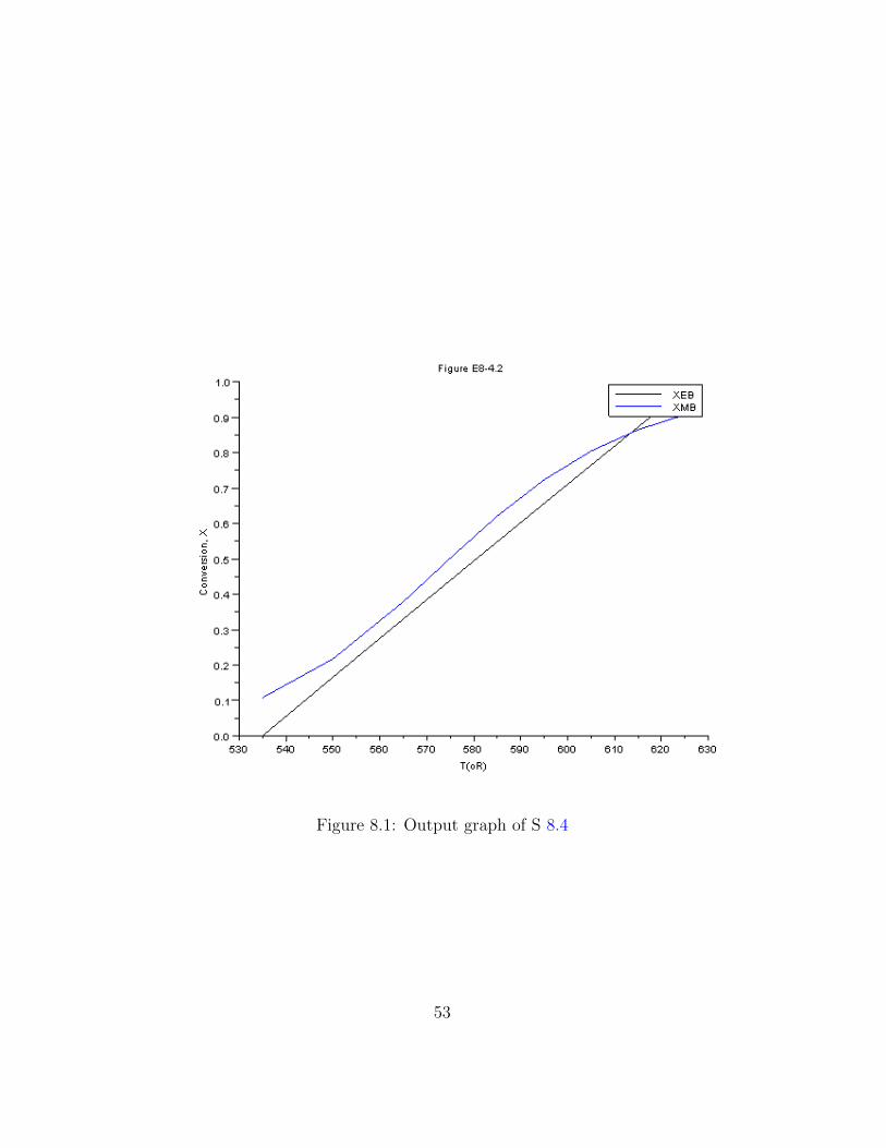
Figure 8.1: Output graph of S 8.4
53
5 function w=f(V,X)
6
7 w =zeros (1,1);
8 T =330+43.3*X;
9 k=31.1* exp (7906*(T -360)/(T*360));
10 Kc = 3.03* exp ( -830.3*((T-360)/(T*360)));
11 Xe = Kc/(1+Kc);
12 ra = -k*Ca0 *(1 -(1+(1/Kc))*X);
13 w(1)= -ra/Fa0;
14 rate = -ra;
15 endfunction
16
17 x=ode([0],V0,V,f);
18
19 for i =1: length(x)
20 T(1,i) =330+43.3*x(1,i)
21
22 k(1,i)=31.1* exp (7906*(T(1,i) -360)/(T(1,i)*360));
23 Kc(1,i) = 3.03* exp ( -830.3*((T(1,i) -360)/(T(1,i)
*360)));
24
25 ra(1,i) = k(1,i)*Ca0 *(1 -(1+(1/Kc(1,i)))*x(1,i));
26 end
27 scf (1)
28 plot2d(V,x(1,:));
29
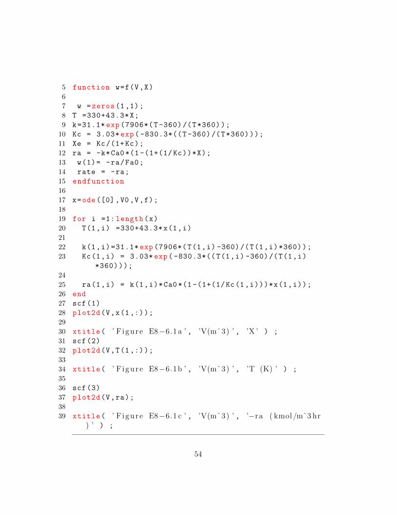
30 xtitle( ’ F i gu r e E8−6.1 a ’ , ’V(mˆ3) ’ , ’X ’ ) ;
31 scf (2)
32 plot2d(V,T(1,:));
33
34 xtitle( ’ F i gu r e E8−6.1b ’ , ’V(mˆ3) ’ , ’T (K) ’ ) ;
35
36 scf (3)
37 plot2d(V,ra);
38
39 xtitle( ’ F i gu r e E8−6.1 c ’ , ’V(mˆ3) ’ , ’−ra ( kmol /mˆ3 hr) ’ ) ;
54
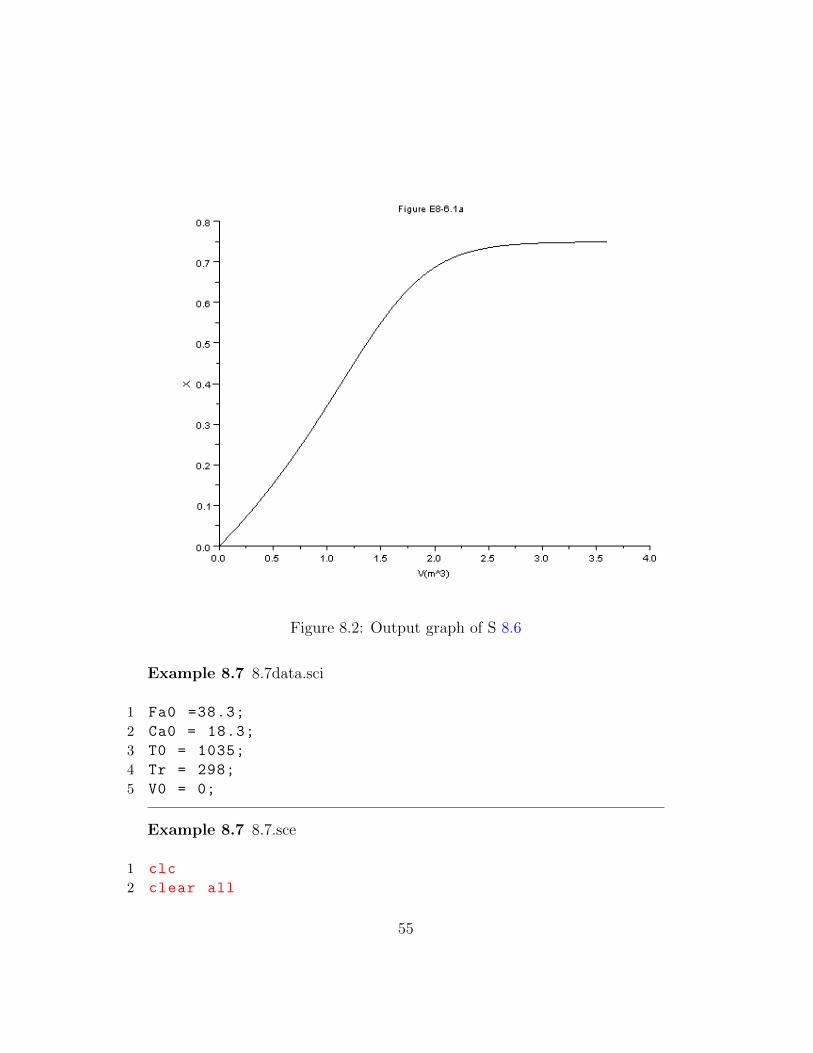
Figure 8.2: Output graph of S 8.6
Example 8.7 8.7data.sci
1 Fa0 =38.3;
2 Ca0 = 18.3;
3 T0 = 1035;
4 Tr = 298;
5 V0 = 0;
Example 8.7 8.7.sce
1 clc
2 clear all
55
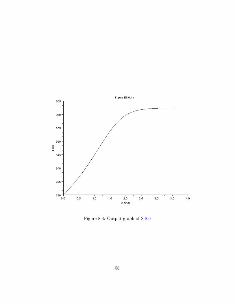
Figure 8.3: Output graph of S 8.6
56
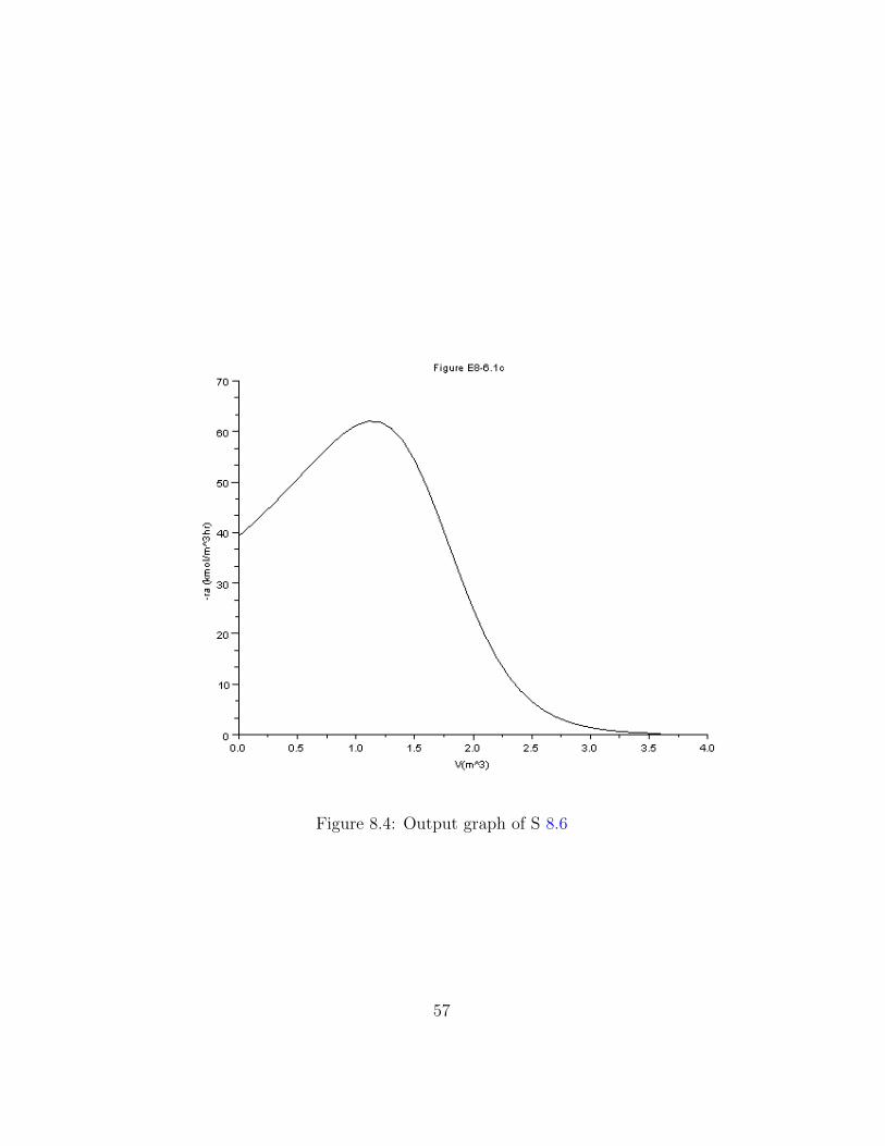
Figure 8.4: Output graph of S 8.6
57
3 // t h i s code i s on ly f o r the f i r s t pa r t o f theproblem ( A d i a b a t i c PFR)
4 exec(” 8 . 7 data . s c i ”);5 V = 0:.1:5;
6 function w=f(V,Y)
7
8 w =zeros (2,1);
9
10 k=(8.2 e14)*exp ( -34222/Y(1));
11
12 Cpa = 26.63+.183*Y(1) -(45.86e-6)*(Y(1) ^2);
13 delCp = 6.8 -(11.5e-3)*Y(1) -(3.81e-6)*(Y(1) ^2);
14 deltaH = 80770+6.8*(Y(1)-Tr) -(5.75e-3) *((Y(1)^2)-Tr
^2) -(1.27e-6) *((Y(1)^3)-Tr^3);
15 ra = -k*Ca0 *(((1 -Y(2))/(1+Y(2)))*(T0/Y(1)));
16 w(1) = -ra*(-deltaH)/(Fa0*(Cpa+Y(2)*delCp));
17 w(2)= -ra/Fa0;
18
19 endfunction
20
21 x=ode ([1035;0] ,V0,V,f);
22 scf (1)
23 plot2d(V,x(1,:));
24
25 xtitle( ’ F i gu r e E8−7.1 ’ , ’V (mˆ3) ’ , ’T (K) ’ ) ;
26
27 scf (2)
28 plot2d(V,x(2,:));
29
30 xtitle( ’ F i gu r e E8−7.1 ’ , ’V (mˆ3) ’ , ’X ’ ) ;
Example 8.8 8.8data.sci
1 T = [300:10:600] ’;
Example 8.8 8.8.sce
58
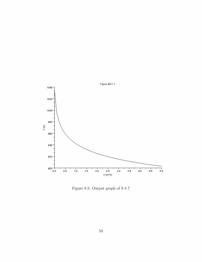
Figure 8.5: Output graph of S 8.7
59
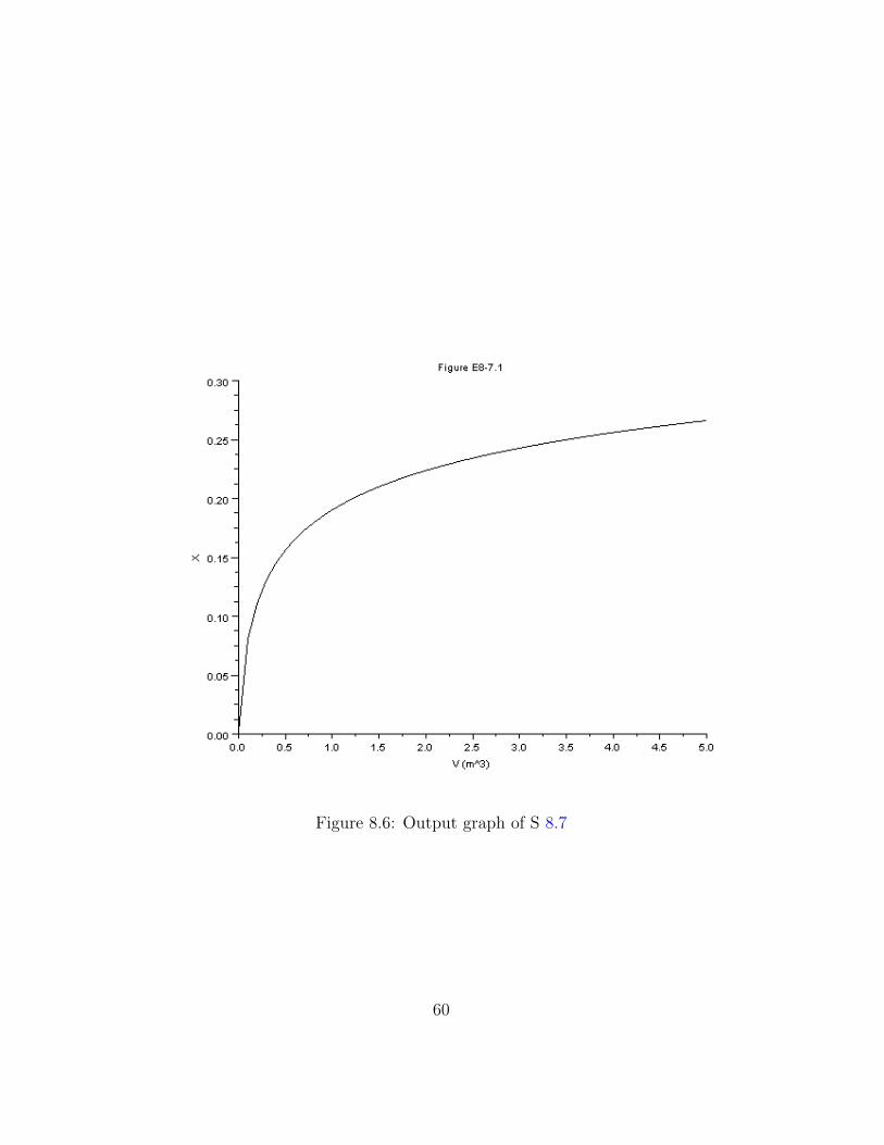
Figure 8.6: Output graph of S 8.7
60
1 clc
2 clear all
3 exec(” 8 . 8 data . s c i ”);4 for i = 1: length(T)
5 Xe(i) = 100000* exp ( -33.78*(T(i) -298)/(T(i)))/(1+
100000* exp ( -33.78*(T(i) -298)/T(i)));
6 XEB(i) = (2.5e-3)*(T(i) -300);
7 end
8 plot2d(T,[Xe XEB])
9
10 xtitle( ’ F i gu r e E8−8.1 ’ , ’T ’ , ’X ’ ) ;
11 legend ([ ’ Xe ’ ; ’XEB ’ ]);
Example 8.10 8.10.sce
1 clc
2 clear all
3 //eY ( 2 ) ec ( ” 8 . 6 data . s c i ” ) ;4 W = 0:1:28.58;
5 W0=0;
6 function w=f(W,Y)
7 w =zeros (3,1);
8
9
10 fao =.188
11 visc =.090
12 Ta =1264.67
13 deltah = -42471 -1.563*(Y(3) -1260) +.00136*(Y(3)
**2 -1260**2) -(2.459*10**( -7))*(Y(3) **3 -1260**3);
14 summ= 57.23+.014 * Y(3) -1.94 *10**( -6.)*Y(3)**2
15 dcp = -1.5625+2.72*10**( -3)*Y(3) -7.38*10**( -7)*Y(3)**2
16 k=360D*exp ( -176008/Y(3) -(110.1* log(Y(3)))+912.8)
17 thetaso =0;
18 Po=2
19 Pao =.22
20 thetao =.91
21 eps =-.055
61
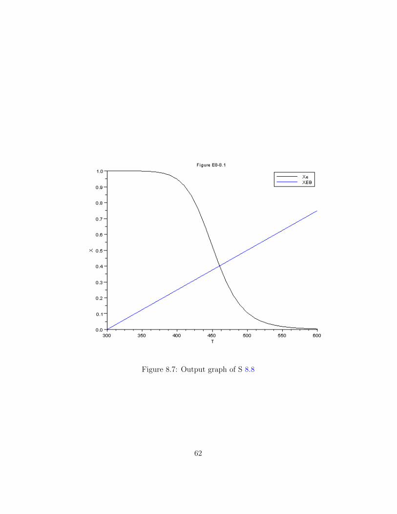
Figure 8.7: Output graph of S 8.8
62
22 R=1.987;
23 Kp=exp (42311/R/Y(3) -11.24);
24 if(Y(2)< =.05)
25
26 ra=(-k*(.848 -.012/( Kp**2)));
27 else
28 ra=(-k*(1-Y(2))/( thetaso+Y(2)))**.5*(Y(1)/Po*Pao
*(( thetao -.5*Y(2))/((1+ eps*Y(2))) -((thetaso+Y
(2))/(1-Y(2)))**2/( Kp**2)));
29 end
30
31 w(1) =( -1.12*10**( -8) *(1 -.055*Y(2))*Y(3))*(5500* visc
+2288)/Y(1) ;
32 w(2)=-(ra)/fao ;
33 w(3) =(5.11*(Ta -Y(3))+(-ra)*(-deltah) )/(fao*(summ+Y
(2)*dcp))
34 endfunction
35
36 X=ode ([2;0;1400] ,W0,W,f);
37
38 plot2d(W,X(1,:));
39 plot2d(W,X(3,:));
Example 8.11 8.11data.sci
1 V0=0;
2 Cto =0.1;
3 To=423;
Example 8.11 8.11.sce
1 clc
2 clear all
3 exec(” 8 . 1 1 data . s c i ”);4 V = 0:.01:1;
5
6 function w=f(V,Y)
63
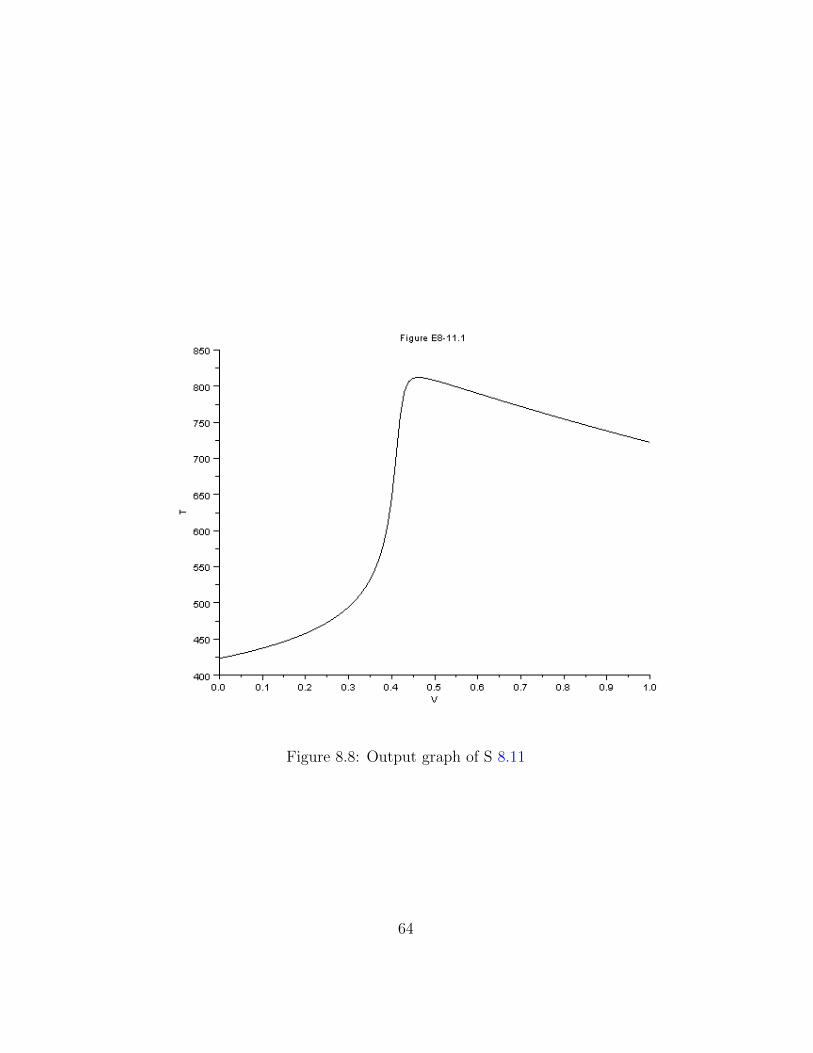
Figure 8.8: Output graph of S 8.11
64
Figure 8.9: Output graph of S 8.11
65
7
8 w =zeros (4,1);
9
10 k1a =10* exp (4000*((1/300) -(1/Y(4))));
11 k2a =.09* exp (9000*((1/300) -(1/Y(4))))
12
13 Ft=Y(1)+Y(2)+Y(3);
14
15 Ca=Cto*(Y(1)/Ft)*(To/Y(4))
16 Cb=Cto*(Y(2)/Ft)*(To/Y(4))
17 Cc=Cto*(Y(3)/Ft)*(To/Y(4))
18 r1a=-k1a*Ca;
19 r2a=-k2a*Ca^2;
20
21 w(1)=r1a+r2a;
22 w(2)=-r1a;
23
24 w(3)=-r2a /2;
25 w(4) =(4000*(373 -Y(4))+(-r1a)*20000+( - r2a)*60000)
/(90*Y(1) +90*Y(2) +180*Y(3));
26 endfunction
27
28 x=ode ([100;0;0;423] ,V0,V,f);
29
30 scf (1)
31 plot2d(V,x(4,:));
32
33 xtitle( ’ F i gu r e E8−11.1 ’ , ’V ’ , ’T ’ ) ;
34
35 scf (2)
36
37 l1=x(1,: )’
38 l2=x(2,: )’
39 l3=x(3,: )’
40 plot2d(V’,[l1 l2 l3]);
41
42 xtitle( ’ F i gu r e E8−11.2 ’ , ’V ’ , ’ Fa , Fb , Fc ’ ) ;
43 legend ([ ’ Fa ’ ; ’Fb ’ ; ’ Fc ’ ]);
66
Example 8.12 8.12data.sci
1 Cp=200
2 Cao =0.3
3 To=283
4 tau =.01;
5 DH1 = -55000;
6 DH2 = -71500;
7 vo =1000;
8 E2 =27000;
9 E1 =9900;
10 UA =40000;
11 Ta=330;
Example 8.12 8.12.sce
1 clc
2 clear all
3 exec(” 8 . 1 2 data . s c i ”);4 t=1:10:250;
5 for i=1: length(t)
6 T(i)=2*t(i)+283;
7
8 k2(i)=4.58* exp((E2 /1.987) *((1/500) -(1/T(i))))
9 k1(i)=3.3* exp((E1 /1.987) *((1/300) -(1/T(i))))
10 Ca(i)=Cao /(1+ tau*k1(i))
11 kappa=UA/(vo*Cao)/Cp
12 G(i)=-(tau*k1(i)/(1+k1(i)*tau))*DH1 -(k1(i)*tau*k2(i)
*tau*DH2 /((1+ tau*k1(i)) *(1+ tau*k2(i))));
13 Tc=(To+kappa*Ta)/(1+ kappa);
14 Cb(i)=tau*k1(i)*Ca(i)/(1+k2(i)*tau);
15 R(i)=Cp*(1+ kappa)*(T(i)-Tc);
16 Cc=Cao -Ca(i)-Cb(i);
17 F(i)=G(i)-R(i);
18 end
19 plot(T’,[G R])
67
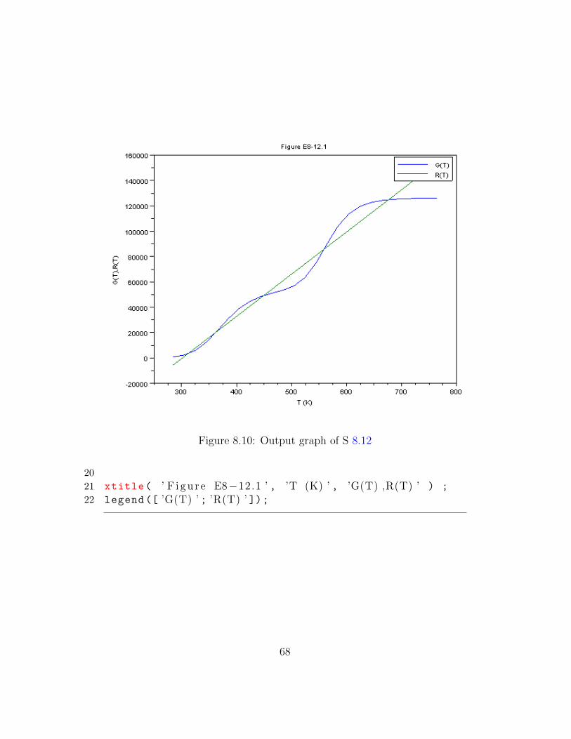
Figure 8.10: Output graph of S 8.12
20
21 xtitle( ’ F i gu r e E8−12.1 ’ , ’T (K) ’ , ’G(T) ,R(T) ’ ) ;
22 legend ([ ’G(T) ’ ; ’R(T) ’ ]);
68
Chapter 9
Unsteady State NonisothermalReactor Design
9.1 Discussion
When executing the code from the editor, use the ’Execute File into Scilab’taband not the ’Load in Scilab’tab. The .sci files of the respective problems con-tain the input parameters of the question
9.2 Scilab Code
Example 9.1 9.1data.sci
1 t0=0;
Example 9.1 9.1.sce
1 clc
2 clear all
3 exec(” 9 . 1 data . s c i ”);4 t = 0:10:1500;
5 function w=f(t,x)
6
7 w =zeros (1,1);
69
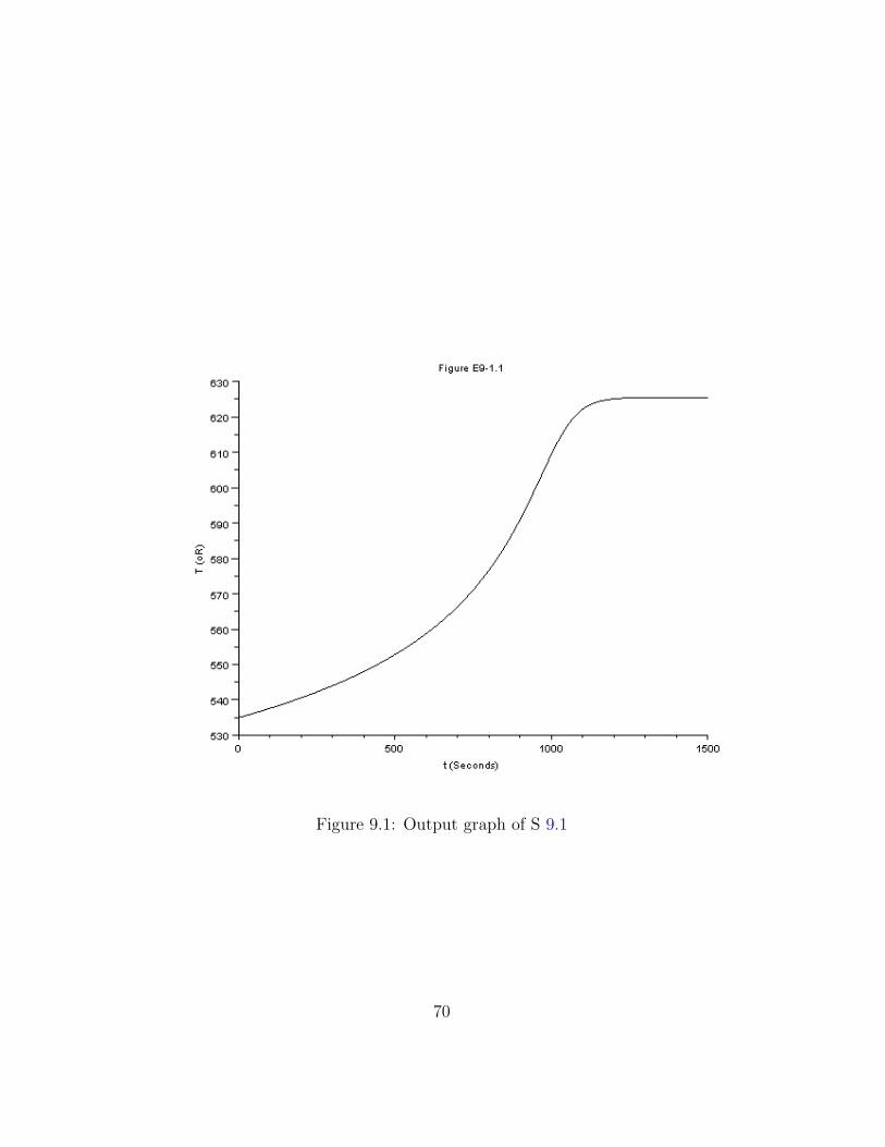
Figure 9.1: Output graph of S 9.1
70
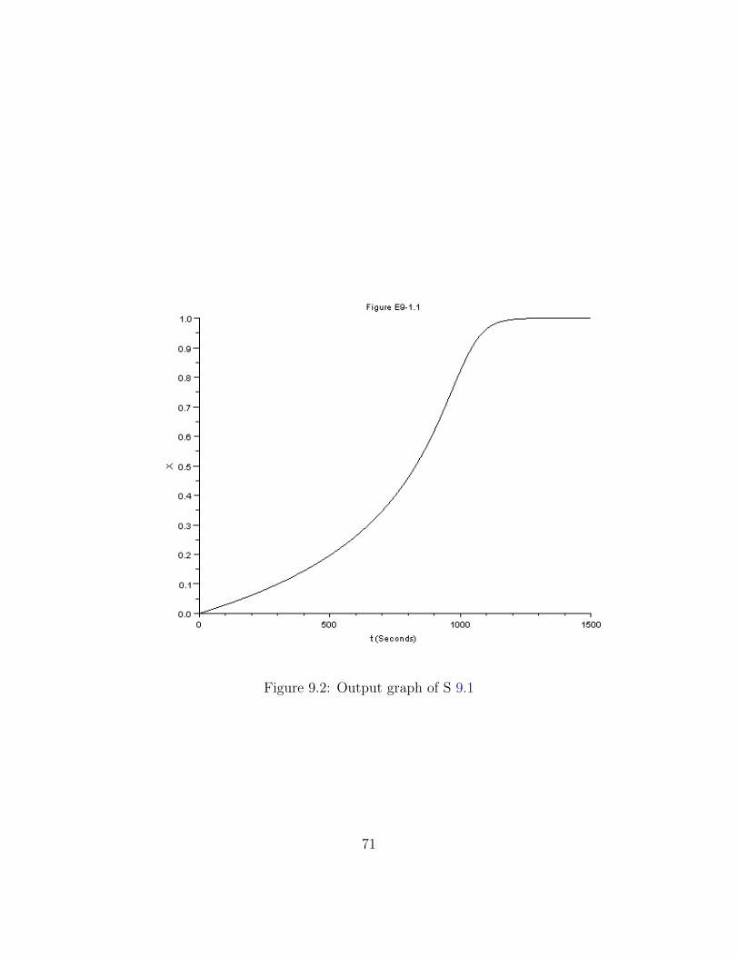
Figure 9.2: Output graph of S 9.1
71
8
9 t1 =535+90.45*x
10 k= .000273* exp (16306*((1/535) -(1/t1)));
11 w(1)=k*(1-x)
12 endfunction
13
14 X=ode([0],t0 ,t,f);
15 T=535+90.45*X;
16 scf (1)
17 plot2d(t,T);
18
19 xtitle( ’ F i gu r e E9−1.1 ’ , ’ t ( Seconds ) ’ , ’T (oR) ’ ) ;
20
21 scf (2)
22 plot2d(t,X);
23
24 xtitle( ’ F i gu r e E9−1.1 ’ , ’ t ( Seconds ) ’ , ’X ’ ) ;
Example 9.2 9.2data.sci
1 NCp =2504;
2 U=3.265+1.854;
3 Nao =9.0448;
4 UA =35.83;
5 dH= -590000;
6 Nbo =33;
7 t0=55;
Example 9.2 9.2.sce
1 clc
2 clear all
3 // t h i s code i s on ly f o r Part C4 exec(” 9 . 2 data . s c i ”);5 t = 55:1:121;
6 function w=f(t,Y)
7
72
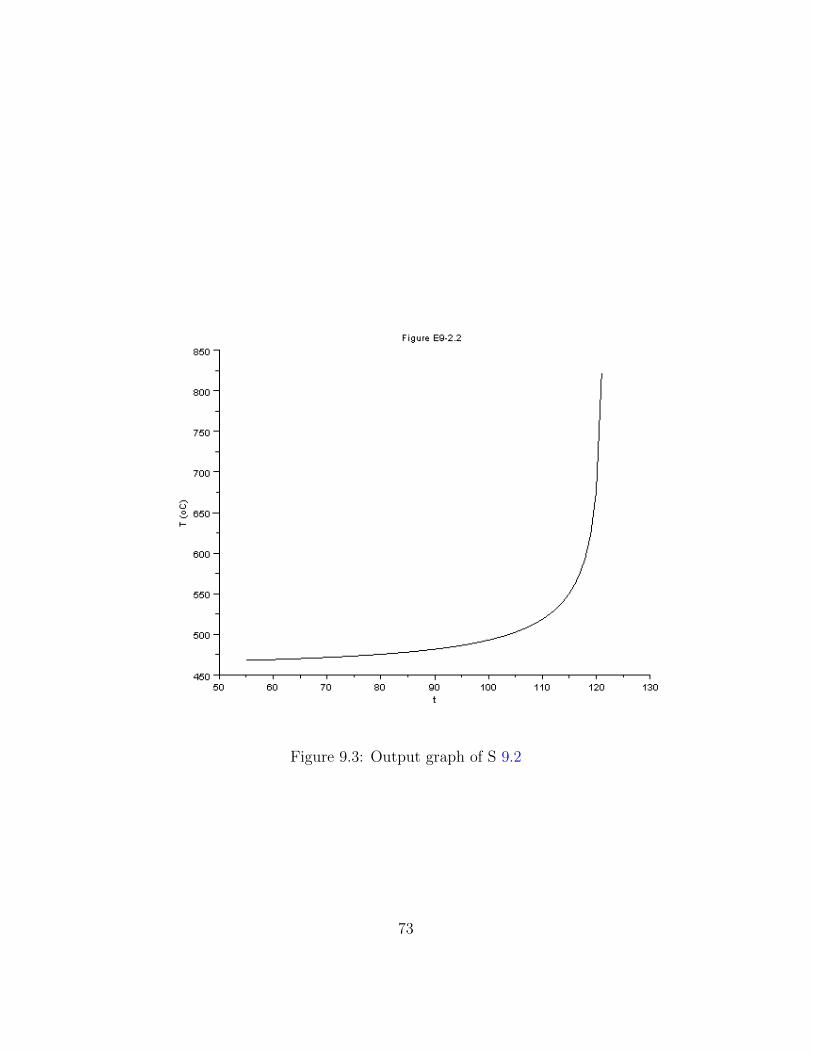
Figure 9.3: Output graph of S 9.2
73
8 w =zeros (2,1);
9
10
11
12 k=.00017* exp (11273/(1.987) *(1/461 -1/Y(1)))
13 Qr=UA*(Y(1) -298)
14 Theata=Nbo/Nao
15 ra=-k*(Nao **2)*(1-Y(2))*(Theata -2*Y(2))/(U**2)
16 rate=-ra
17 Qg=ra*U*(dH)
18 w(1)=(Qg-Qr)/NCp
19 w(2)=(-ra)*U/Nao
20 endfunction
21
22 x=ode ([467.992;0.0423] ,t0 ,t,f);
23
24
25 plot2d(t,x(1,:));
26
27 xtitle( ’ F i gu r e E9−2.2 ’ , ’ t ’ , ’T (oC) ’ ) ;
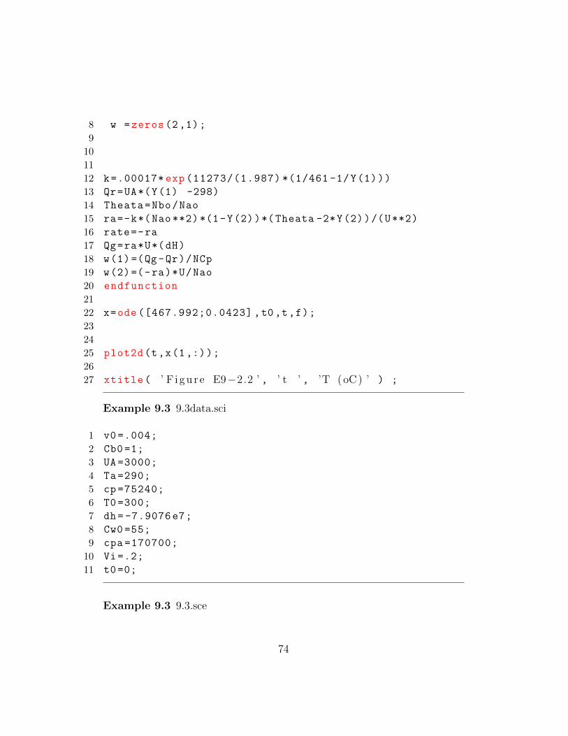
Example 9.3 9.3data.sci
1 v0 =.004;
2 Cb0 =1;
3 UA =3000;
4 Ta=290;
5 cp =75240;
6 T0=300;
7 dh= -7.9076e7;
8 Cw0 =55;
9 cpa =170700;
10 Vi=.2;
11 t0=0;
Example 9.3 9.3.sce
74
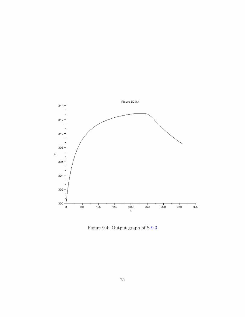
Figure 9.4: Output graph of S 9.3
75
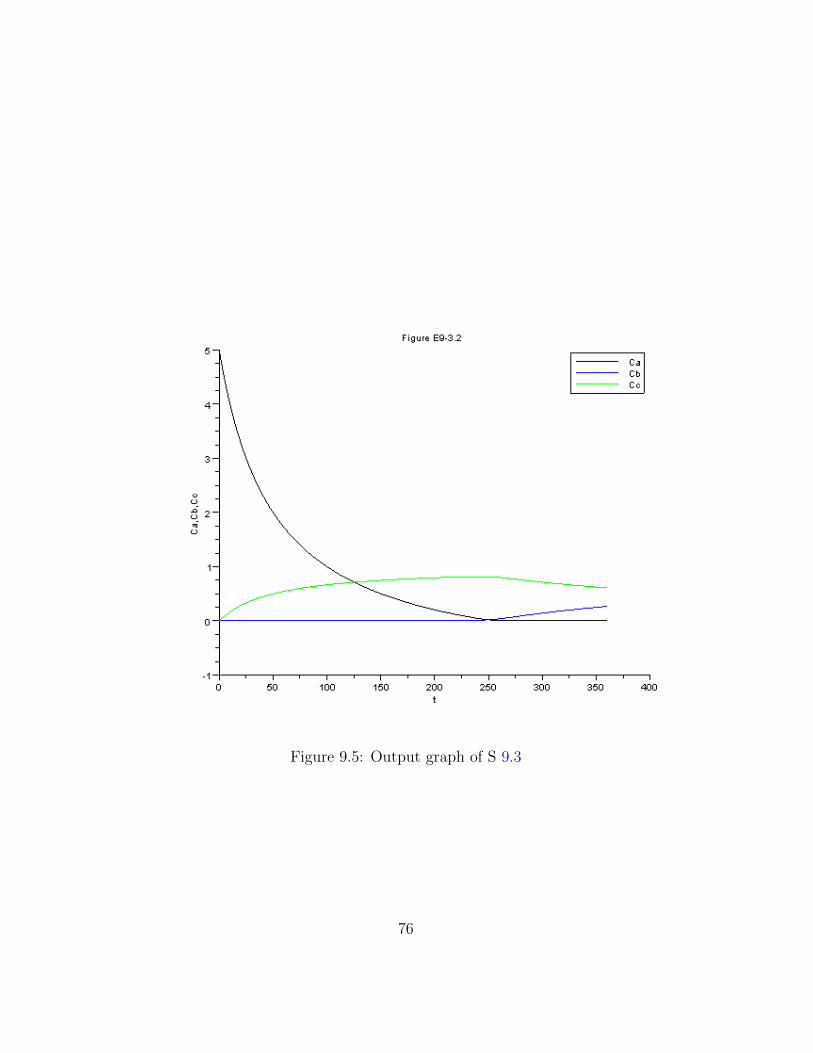
Figure 9.5: Output graph of S 9.3
76
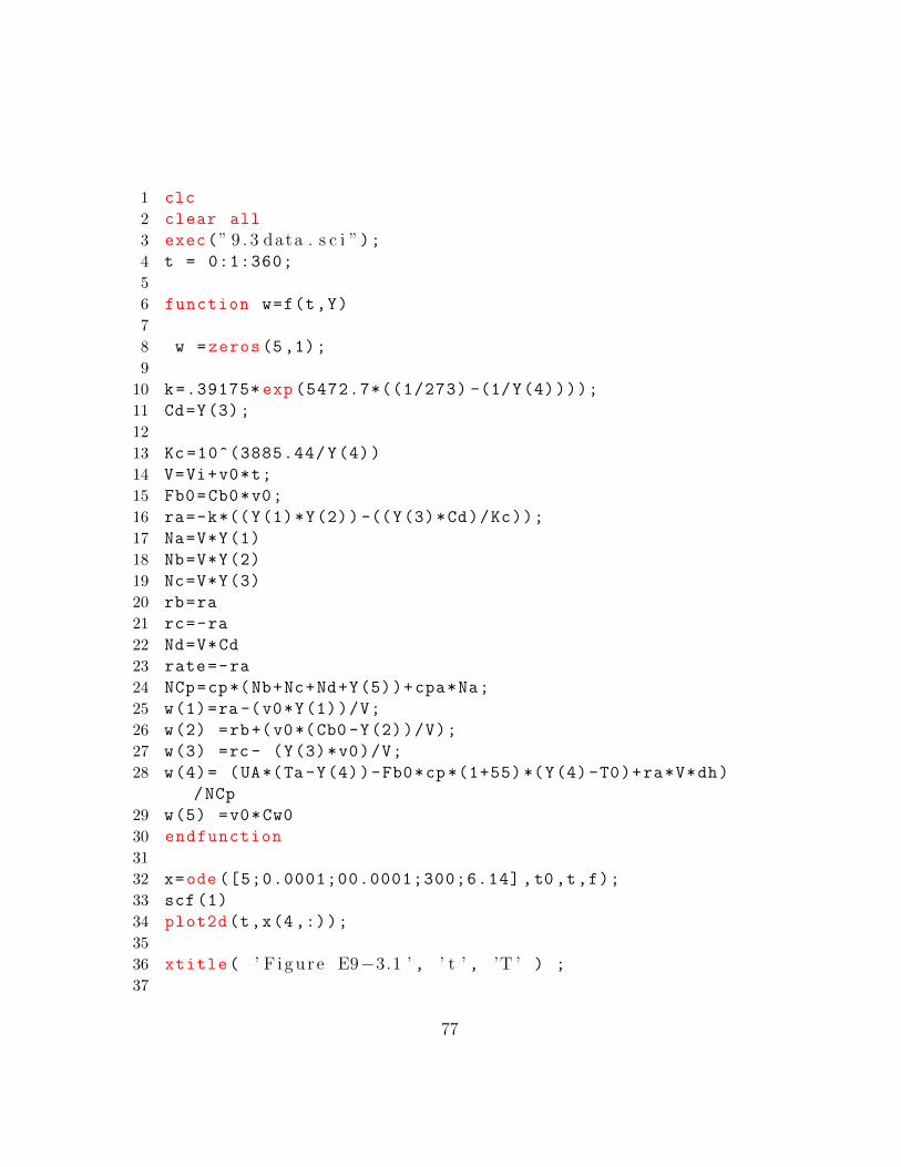
1 clc
2 clear all
3 exec(” 9 . 3 data . s c i ”);4 t = 0:1:360;
5
6 function w=f(t,Y)
7
8 w =zeros (5,1);
9
10 k=.39175* exp (5472.7*((1/273) -(1/Y(4))));
11 Cd=Y(3);
12
13 Kc =10^(3885.44/Y(4))
14 V=Vi+v0*t;
15 Fb0=Cb0*v0;
16 ra=-k*((Y(1)*Y(2)) -((Y(3)*Cd)/Kc));
17 Na=V*Y(1)
18 Nb=V*Y(2)
19 Nc=V*Y(3)
20 rb=ra
21 rc=-ra
22 Nd=V*Cd
23 rate=-ra
24 NCp=cp*(Nb+Nc+Nd+Y(5))+cpa*Na;
25 w(1)=ra -(v0*Y(1))/V;
26 w(2) =rb+(v0*(Cb0 -Y(2))/V);
27 w(3) =rc - (Y(3)*v0)/V;
28 w(4)= (UA*(Ta-Y(4))-Fb0*cp *(1+55) *(Y(4)-T0)+ra*V*dh)
/NCp
29 w(5) =v0*Cw0
30 endfunction
31
32 x=ode ([5;0.0001;00.0001;300;6.14] ,t0 ,t,f);
33 scf (1)
34 plot2d(t,x(4,:));
35
36 xtitle( ’ F i gu r e E9−3.1 ’ , ’ t ’ , ’T ’ ) ;
37
77
38 scf (2)
39 l1=x(1,: )’
40 l2=x(2,: )’
41 l3=x(3,: )’
42 plot2d(t’,[l1 l2 l3]);
43
44 xtitle( ’ F i gu r e E9−3.2 ’ , ’ t ’ , ’Ca , Cb , Cc ’ ) ;
45 legend ([ ’Ca ’ ; ’Cb ’ ; ’ Cc ’ ]);
Example 9.4 9.4data.sci
1 Fa0 =80;
2 T0=75;
3 V=(1/7.484) *500;
4 UA =16000;
5 Ta1 =60;
6 Fb0 =1000;
7 Fm0 =100;
8 mc =1000;
9 t0=0;
Example 9.4 9.4.sce
1 clc
2 clear all
3 // exec ( ” 9 . 3 data . s c i ” ) ;4 t = 0:.0001:4;
5 t0=0;
6 function w=f(t,Y)
7
8 w =zeros (5,1);
9
10 Fa0 =80;
11 T0=75;
12 V=(1/7.484) *500;
13 UA =16000;
14 Ta1 =60;
15 k=16.96 e12*exp ( -32400/1.987/(Y(5) +460));
78
16 Fb0 =1000;
17 Fm0 =100;
18 mc =1000;
19 ra=-k*Y(1);
20 rb=-k*Y(1);
21 rc=k*Y(1) ;
22 Nm=Y(4)*V;
23 Na=Y(1)*V;
24 Nb=Y(2)*V;
25 Nc=Y(3)*V;
26 ThetaCp =35+( Fb0/Fa0)*18+( Fm0/Fa0)*19.5;
27 v0=(Fa0 /0.923) +(Fb0 /3.45) +(Fm0 /1.54);
28 Ta2=Y(5)- (Y(5)-Ta1)*exp (-UA/(18*mc));
29 Ca0=Fa0/v0
30 Cb0=Fb0/v0
31 Cm0=Fm0/v0
32 Q=mc*18*(Ta1 -Ta2);
33 tau=V/v0;
34 NCp=Na*35+Nb*18+Nc*46+Nm *13.5;
35 w(1) =(1/ tau)*(Ca0 -Y(1))+ra;
36 w(2) =(1/ tau)*(Cb0 -Y(2))+rb;
37 w(3) =(1/ tau)*(-Y(3))+rc;
38 w(4) =(1/ tau)*(Cm0 -Y(4));
39 w(5) = (Q-Fa0*ThetaCp *(Y(5)-T0)+( -36000)*ra*V)/NCp;
40 endfunction
41
42 x=ode ([0;3.45;0;0;75] ,t0 ,t,f);
43 scf (1)
44 plot2d(t,x(1,:));
45
46 xtitle( ’ F i gu r e E9−4.1 ’ , ’ t ’ , ’Ca ’ ) ;
47
48 scf (2)
49 plot2d(t,x(5,:));
50
51 xtitle( ’ F i gu r e E9−4.2 ’ , ’ t ’ , ’T ’ ) ;
52 scf (3)
53 plot2d(x(5,:),x(1,:));
79
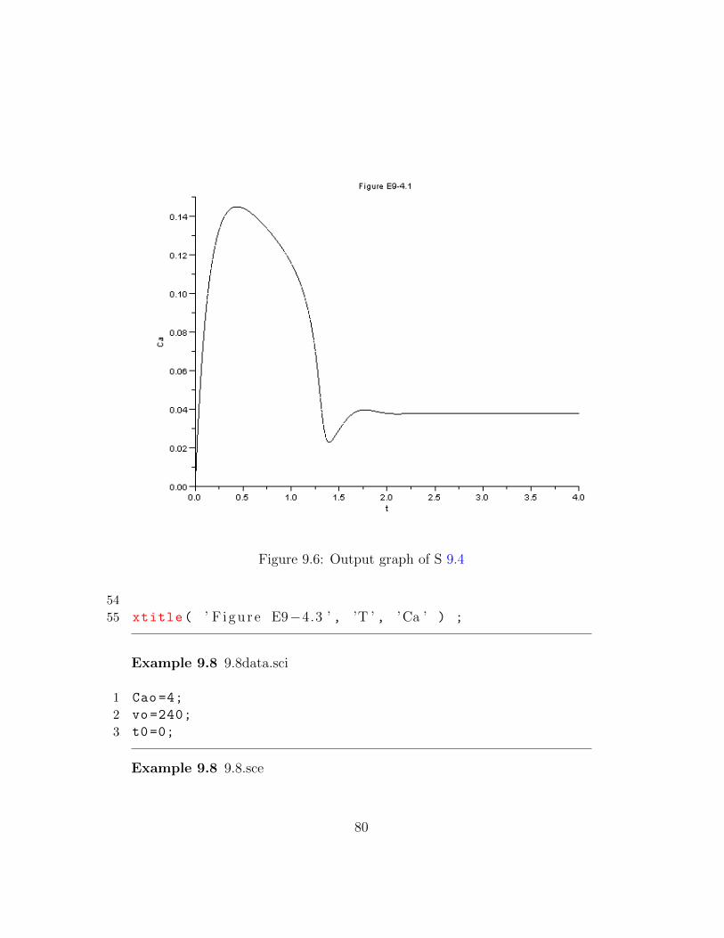
Figure 9.6: Output graph of S 9.4
54
55 xtitle( ’ F i gu r e E9−4.3 ’ , ’T ’ , ’Ca ’ ) ;
Example 9.8 9.8data.sci
1 Cao =4;
2 vo=240;
3 t0=0;
Example 9.8 9.8.sce
80
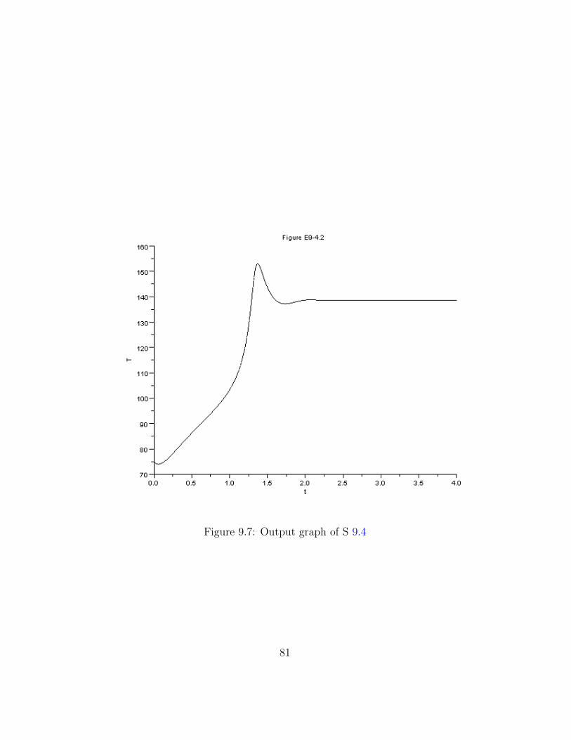
Figure 9.7: Output graph of S 9.4
81
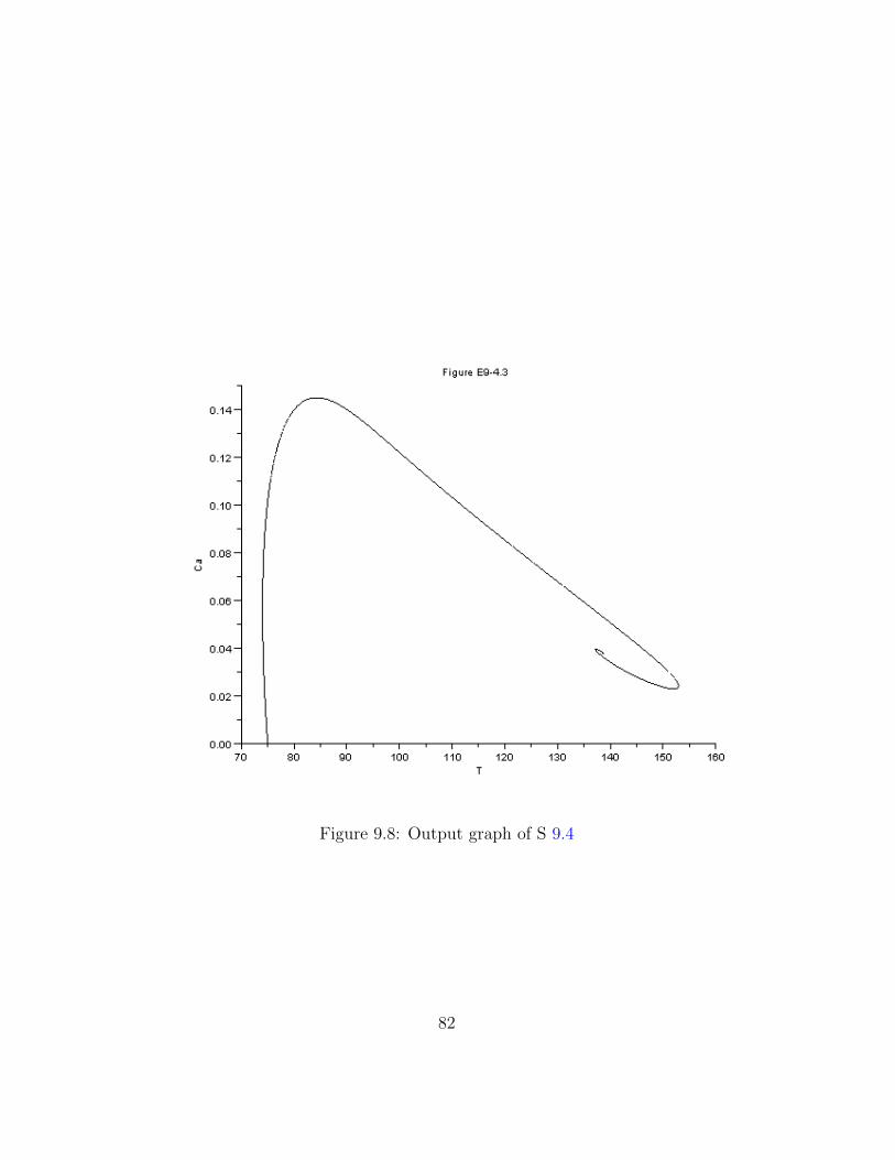
Figure 9.8: Output graph of S 9.4
82
1 clc
2 clear all
3 exec(” 9 . 8 data . s c i ”);4 t = 0:.01:1.5;
5
6 function w=f(t,Y)
7
8 w =zeros (4,1);
9
10 k1a =1.25* exp ((9500/1.987) *((1/320) -(1/Y(4))));
11 k2b =0.08* exp ((7000/1.987) *((1/290) -(1/Y(4))));
12 ra=-k1a*Y(1);
13 V=100+ vo*t;
14 rc=3*k2b*Y(2);
15 rb=k1a*(Y(1)/2)-k2b*Y(2);
16 w(1)=ra+(Cao -Y(1))*vo/V;
17 w(2)=rb-Y(2)*vo/V;
18 w(3)=rc-Y(3)*vo/V; w(4) =(35000*(298 -Y(4))-Cao*vo
*30*(Y(4) -305) +(( -6500)*(-k1a*Y(1))+(8000)*(-k2b*
Y(2)))*V)/((Y(1) *30+Y(2) *60+Y(3) *20)*V+100*35);
19 endfunction
20
21 x=ode ([1;0;0;290] ,t0,t,f);
22
23
24 scf (1)
25 l1=x(1,: )’
26 l2=x(2,: )’
27 l3=x(3,: )’
28 plot2d(t’,[l1 l2 l3]);
29
30 xtitle( ’ F i gu r e E9−8.1 ’ , ’ t ’ , ’Ca , Cb , Cc ’ ) ;
31 legend ([ ’Ca ’ ; ’Cb ’ ; ’ Cc ’ ]);32
33 scf (2)
34 plot2d(t,x(4,:));
35
36 xtitle( ’ F i gu r e E9−8.2 ’ , ’ t ’ , ’T ’ ) ;
83
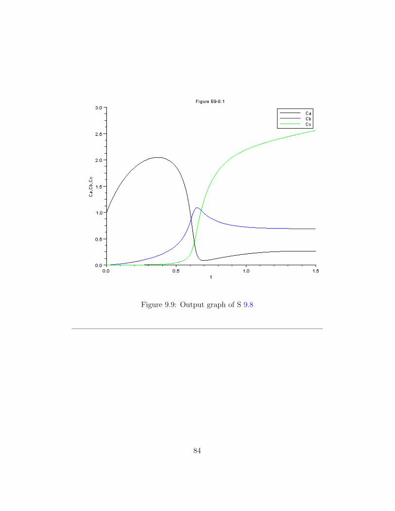
Figure 9.9: Output graph of S 9.8
84
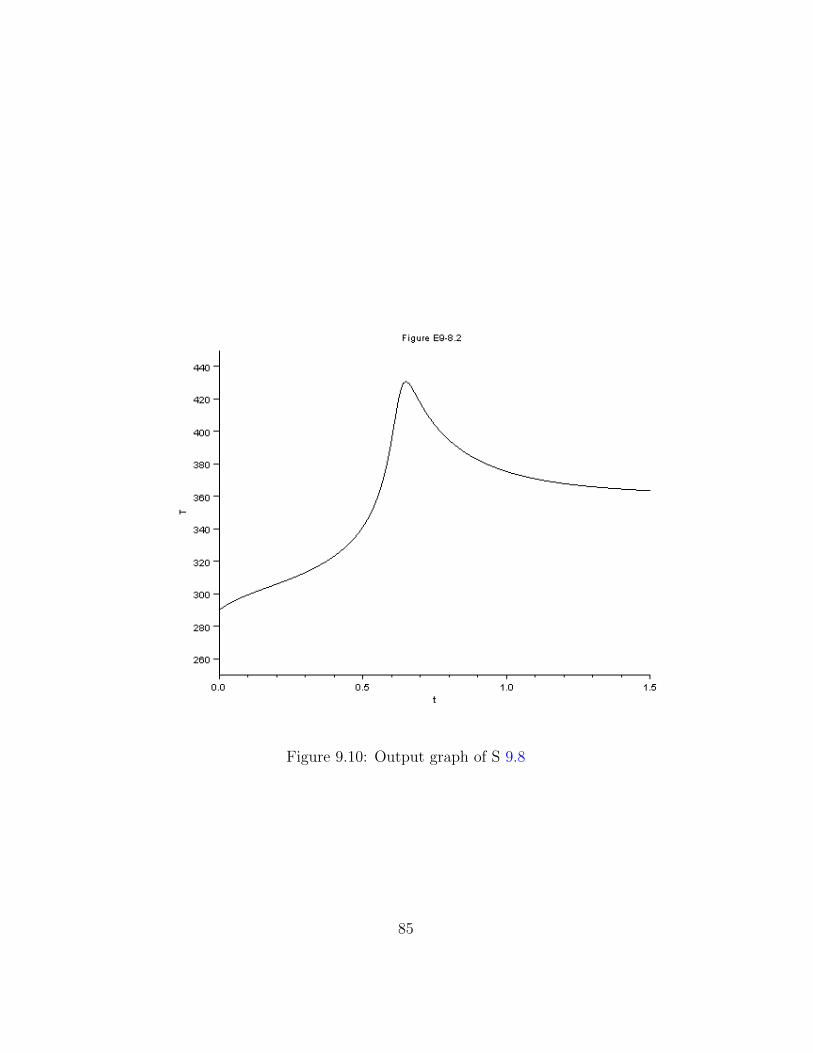
Figure 9.10: Output graph of S 9.8
85
Chapter 10
Catalysis and CatalyticReactors
10.1 Discussion
When executing the code from the editor, use the ’Execute File into Scilab’taband not the ’Load in Scilab’tab. The .sci files of the respective problems con-tain the input parameters of the question
10.2 Scilab Code
Example 10.3 10.3data.sci
1 ftO =50
2 k=.0000000145*1000*60;
3 kt =1.038;
4 kb =1.39;
5 alpha =0.000098;
6 Po=40;
7 w0=0;
Example 10.3 10.3.sce
1 clc
2 clear all
86
3 exec(” 1 0 . 3 data . s c i ”);4 w = 0:10:10000;
5
6 function W=f(w,x)
7
8 W =zeros (1,1);
9
10 pt0 =.3*Po;
11 y=(1- alpha*w)^.5;
12 ph=pt0*(1.5-x)*y;
13 pt=pt0*(1-x)*y;
14 pb=2*pt0*x*y;
15 rt=-k*kt*ph*pt/(1+kb*pb+kt*pt);
16 rate=-rt;
17 W(1)=-rt/ftO;
18 endfunction
19 pt0 =.3*Po;
20 X=ode([0],w0 ,w,f);
21
22
23 for i =1: length(X)
24 y(1,i)=(1-alpha*w(1,i))^.5;
25 ph(1,i)=pt0 *(1.5 -X(1,i))*y(1,i);
26 pt(1,i)=pt0*(1-X(1,i))*y(1,i);
27 pb(1,i)=2* pt0*X(1,i)*y(1,i)
28 end
29
30 m1 = X’;
31 m2=y’;
32 scf (1)
33 plot2d(w’,[m1 m2]);
34
35 xtitle( ’ F i gu r e E10−3.1 ’ , ’w ’ , ’ x , y ’ ) ;
36 legend ([ ’ x ’ ; ’ y ’ ]);37
38 scf (2)
39 l1=ph’
40 l2=pt’
87
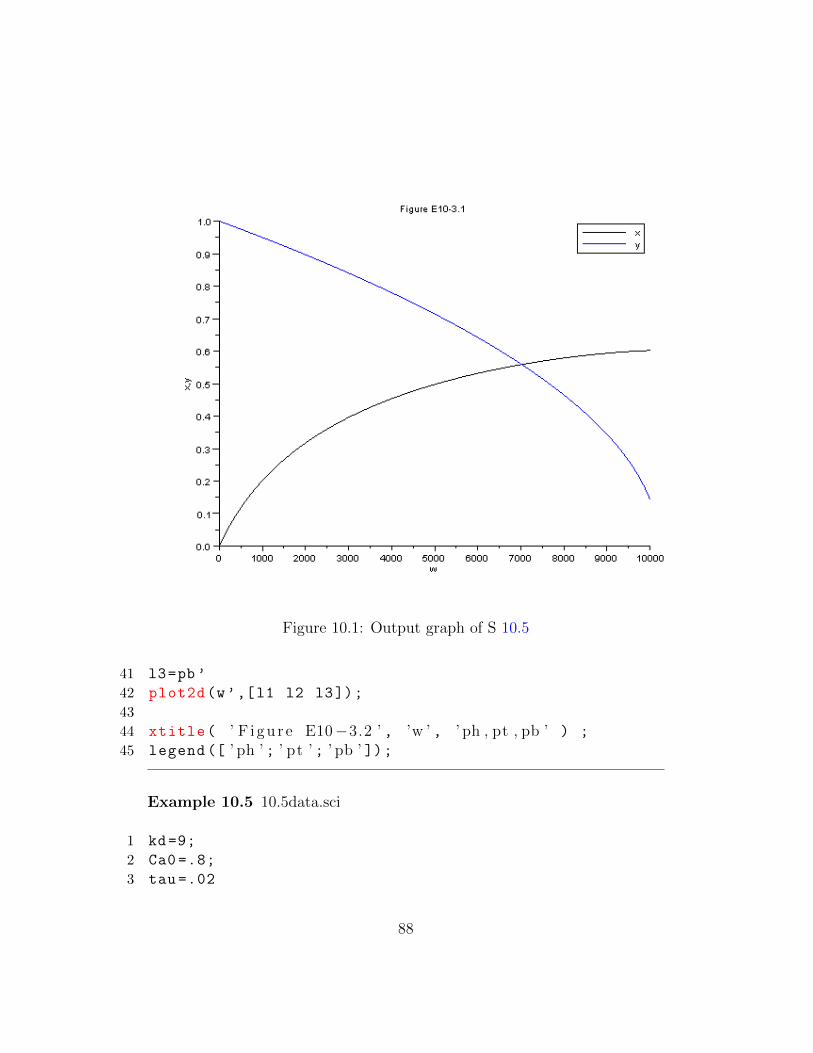
Figure 10.1: Output graph of S 10.5
41 l3=pb’
42 plot2d(w’,[l1 l2 l3]);
43
44 xtitle( ’ F i gu r e E10−3.2 ’ , ’w ’ , ’ ph , pt , pb ’ ) ;
45 legend ([ ’ ph ’ ; ’ pt ’ ; ’ pb ’ ]);
Example 10.5 10.5data.sci
1 kd=9;
2 Ca0 =.8;
3 tau =.02
88
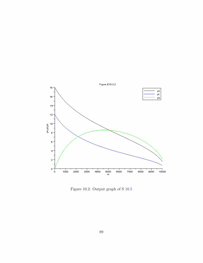
Figure 10.2: Output graph of S 10.5
89
4 k=45;
5 Ct0 =1;
6 t0=0
Example 10.5 10.5.sce
1 clc
2 clear all
3 exec(” 1 0 . 5 data . s c i ”);4 t = 0:.01:.5;
5
6 function w=f(t,Y)
7
8 w =zeros (2,1);
9
10
11 ya0=Ca0/Ct0;
12 X=1-(1+ya0)/(1+Y(2)/Ct0)*Y(2)/Ca0;
13 w(1)=-kd*Y(1)*Y(2);
14 w(2) = (Ca0/tau) -((1+ya0)/(1+(Y(2)/Ct0))+tau*Y(1)*k)
*Y(2)/tau;
15 endfunction
16
17 x=ode ([1;.8] ,t0 ,t,f);
18 Ca0 =.8;
19 Ct0=1
20 ya0=Ca0/Ct0;
21 for i=1: length(t)
22 X1(i)=1 -(1+ ya0)/(1+x(2,i)/Ct0)*x(2,i)/Ca0;
23 end
24
25
26 l1=x(1,: )’
27 l2=x(2,: )’
28 l3=X1;
29 plot2d(t’,[l1 l2 l3]);
30
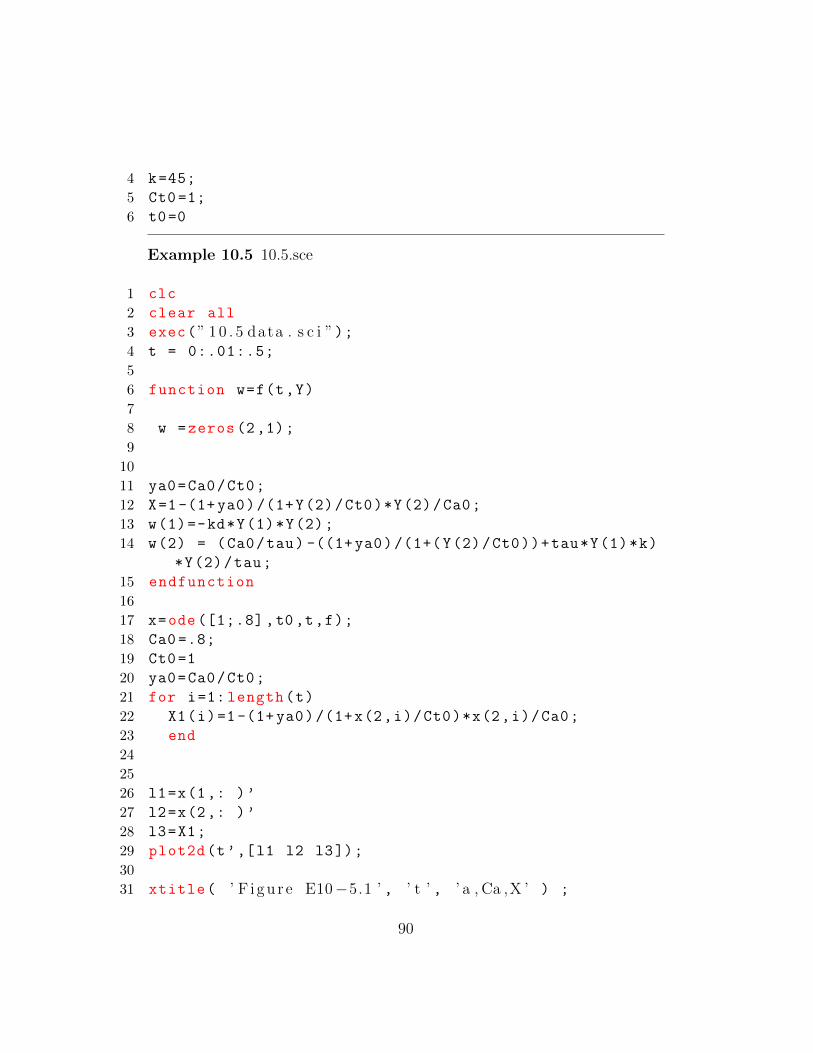
31 xtitle( ’ F i gu r e E10−5.1 ’ , ’ t ’ , ’ a , Ca ,X ’ ) ;
90
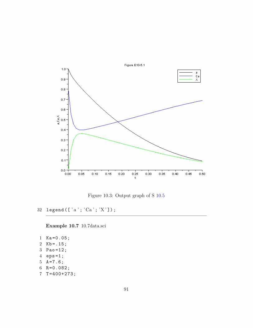
Figure 10.3: Output graph of S 10.5
32 legend ([ ’ a ’ ; ’Ca ’ ; ’X ’ ]);
Example 10.7 10.7data.sci
1 Ka =0.05;
2 Kb=.15;
3 Pao =12;
4 eps =1;
5 A=7.6;
6 R=0.082;
7 T=400+273;
91
8 Kc=.1;
9 rho =80;
10 kprime =0.0014;
11 D=1.5;
12 Uo=2.5;
Example 10.7 10.7.sce
1 clc
2 clear all
3 exec(” 1 0 . 7 data . s c i ”);4 z = 0:.1:10;
5 z0=0;
6 function w=f(z,X)
7
8 w =zeros (1,1);
9
10
11 U=Uo*(1+ eps*X)
12 Pa=Pao*(1-X)/(1+ eps*X)
13 Pb=Pao*X/(1+ eps*X)
14 vo=Uo *3.1416*D*D/4
15 Ca0=Pao/R/T
16 Kca=Ka*R*T
17 Pc=Pb
18 a=1/(1+A*(z/U)**0.5)
19 raprime=a*(-kprime*Pa/(1+ Ka*Pa+Kb*Pb+Kc*Pc))
20 ra=rho*raprime;
21 w(1)=-ra/U/Ca0
22 endfunction
23
24 x=ode([0],z0 ,z,f);
25 for i=1: length(z)
26 U(1,i)=Uo*(1+ eps*x(1,i))
27 a(1,i)=1/(1+A*(z(1,i)/U(1,i))**0.5)
28 end
29
30
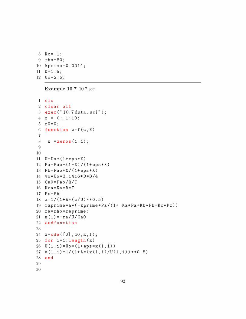
92
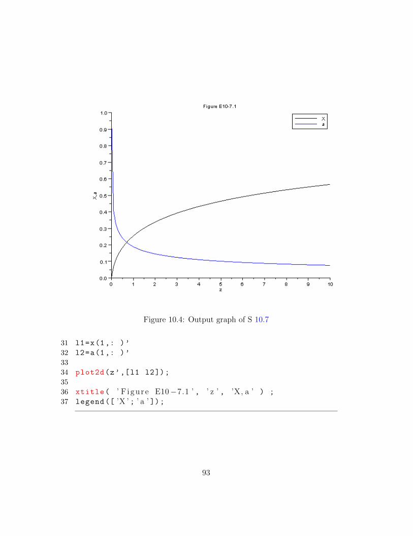
Figure 10.4: Output graph of S 10.7
31 l1=x(1,: )’
32 l2=a(1,: )’
33
34 plot2d(z’,[l1 l2]);
35
36 xtitle( ’ F i gu r e E10−7.1 ’ , ’ z ’ , ’X, a ’ ) ;
37 legend ([ ’X ’ ; ’ a ’ ]);
93
Chapter 11
External Diffusion Effects onHetrogeneous Reactions
11.1 Discussion
When executing the code from the editor, use the ’Execute File into Scilab’taband not the ’Load in Scilab’tab. The .sci files of the respective problems con-tain the input parameters of the question
11.2 Scilab Code
Example 11.1 11.1data.sci
1 DAB =1e-6;
2 CT0 =.1; // kmol /mˆ33 yAb =.9;
4 yAs =.2;
5 s=1e-6;
6 c=.1;
Example 11.1 11.1.sce
1 clc
2 clear all
3 exec(” 1 1 . 1 data . s c i ”);
94
4 WAZ1=DAB*CT0*(yAb -yAs)/s;
5 WAZ2=c*DAB*CT0*log((1-yAs)/(1-yAb))/s;
6 disp(WAZ1)
7 disp(WAZ2)
Example 11.3 11.3data.sci
1 D=.0025; //m2 L=.005; //m3 phi =.3;
4 U=15; //m/ s ;5 v=4.5e-4; //mˆ2/ s6 r=.0025/2;
7 Lp =.005;
8 DAB0 =.69e-4;
9 T=750;
10 T0=298;
11 z=.05; //m
Example 11.3 11.3.sce
1 clc
2 clear all
3 exec(” 1 1 . 3 data . s c i ”);4 // t h i s i s on ly Part A o f the problem .5 dp=(6*(D^2)*L/4) ^(1/3);
6 disp(” P a r t i c l e d i amete r dp =”)7 disp(dp)
8 disp(”m”)9 ac=6*(1- phi)*(1/dp);
10 disp(” S u r f a c e a r ea pervo lume o f bed =”)11 disp(ac)
12 disp(”mˆ2/mˆ3 ”)13 Re =dp*U/v;
14 Y=(2*r*Lp+2*r^2)/dp^2;
15 Reprime=Re/((1-phi)*Y);
16 DAB=DAB0*(T/T0)^(1.75);
17 Sc=v/DAB;
95
18 Shprime =(( Reprime)^.5)*Sc ^(1/3);
19 kc=DAB*(1-phi)*Y*( Shprime)/(dp*phi);
20 X=1-exp(-kc*ac*z/U);
21 disp(”X =”)22 disp(X)
Example 11.4 11.4data.sci
1 X1 =.865;
Example 11.4 11.4.sce
1 clc
2 clear all
3 exec(” 1 1 . 4 data . s c i ”)4 X2=1-(1/ exp((log(1/(1-X1)))*(1/2) *((2) ^.5)));
5 disp(”X2 =”)6 disp(X2)
Example 11.5 11.5data.sci
1 X1 =.865;
2 T1=673;
3 T2=773;
Example 11.5 11.5.sce
1 clc
2 clear all
3 exec(” 1 1 . 5 data . s c i ”)4 X2=1-(1/ exp((log(1/(1-X1)))*((T2/T1)^(5/12))));
5 disp(”X2 =”)6 disp(X2)
96
Chapter 12
Diffusion and Reaction inPours Catalysts
12.1 Discussion
When executing the code from the editor, use the ’Execute File into Scilab’taband not the ’Load in Scilab’tab. The .sci files of the respective problems con-tain the input parameters of the question
12.2 Scilab Code
97
Chapter 13
Distributions of ResidenceTimes for Chemical Reactions
13.1 Discussion
When executing the code from the editor, use the ’Execute File into Scilab’taband not the ’Load in Scilab’tab. The .sci files of the respective problems con-tain the input parameters of the question
13.2 Scilab Code
Example 13.8 13.8data.sci
1 k=0.01
2 cao =8;
3 z0=0;
Example 13.8 13.8.sce
1 clc
2 clear all
3 exec(” 1 3 . 8 data . s c i ”);4 z = 0:1:200;
5
6 function w=f(z,x)
98
7
8 w =zeros (1,1);
9
10 lam=200-z;
11 ca=cao*(1-x)
12 E1 =4.44658e-10*( lam ^4) -1.1802e-7*( lam^3) +1.35358e
-5*( lam^2) -.00086
13 5652* lam +.028004;
14 E2= -2.64e-9*( lam^3) +1.3618e-6*( lam^2) -.00024069* lam
+.015011
15 F1 =4.44658e -10/5*( lam ^5) -1.1802e-7/4* lam ^4+1.35358e
-5/3* lam ^3 -.000865652/2* lam ^2+.028004* lam;
16 F2= -( -9.3076e-8*lam ^3+5.02846e-5*lam ^2 -.00941* lam
+.61823 -1)
17 ra=-k*ca^2;
18 if lam < =70
19 E=E1
20 else
21 E=(E2)
22 end
23 if(lam < =70)
24 F=F1
25 else
26 F=F2
27 end
28 EF=E/(1-F)
29 w(1)=-(ra/cao+E/(1-F)*x)
30 endfunction
31
32 X=ode([0],z0 ,z,f);
33
34 plot2d(z,X);
Example 13.9 13.9data.sci
1 k1=1;
2 k2=1;
3 k3=1;
99
4 t0=0;
Example 13.9 13.8.sce
1 clc
2 clear all
3 exec(” 1 3 . 9 data . s c i ”);4 t = 0:.1:2.52;
5
6 function w=f(t,Y)
7
8 w =zeros (10,1);
9
10 E1= -2.104*t^4+4.167*t^3 -1.596*t^2+0.353*t-.004
11 E2= -2.104*t^4+17.037*t^3 -50.247*t^2+62.964*t -27.402
12 rc=k1*Y(1)*Y(2)
13 re=k3*Y(2)*Y(4)
14 ra=-k1*Y(1)*Y(2)-k2*Y(1)
15 rb=-k1*Y(1)*Y(2)-k3*Y(2)*Y(4)
16 if t< =1.26
17 E=E1
18 else
19 E=E2
20 end
21 rd=k2*Y(1)-k3*Y(2)*Y(4)
22
23 w(1)=ra
24 w(2) =rb
25 w(3) =rc
26 w(6)=Y(1)*E
27 w(7)=Y(2)*E
28 w(8)=Y(3)*E
29 w(4)=rd
30 w(5) =re
31 w(9)=Y(4)*E
32 w(10)=Y(5)*E
33 endfunction
34
100
35 X=ode ([1;1;0;0;0;0;0;0;0;0] ,t0,t,f);
36
37 plot2d(t,X(1,:));
101
Chapter 14
Models for Nonideal Reactors
14.1 Discussion
When executing the code from the editor, use the ’Execute File into Scilab’taband not the ’Load in Scilab’tab. The .sci files of the respective problems con-tain the input parameters of the question
14.2 Scilab Code
Example 14.3 14.3.sce
1 clc
2 clear all
3
4 t = 0:10:200;
5
6 function w=f(t,Y)
7
8 w =zeros (2,1);
9
10 CTe1 =2000 -59.6*t+.64*t^2 -0.00146*t^3 -1.047*10^( -5)*t
^4
11 Beta =.1
12 CTe2 =921 -17.3*t+.129*t^2 -0.000438*t^3+5.6*10^( -7)*t
^4
102
13 alpha =.8
14 tau =40
15 if(t<80)
16 CTe=CTe1
17 else
18 CTe=CTe2
19 end
20
21 w(1)=(Beta*Y(2) -(1+Beta)*Y(1))/alpha/tau
22 w(2)=(Beta*Y(1)-Beta*Y(2))/(1-alpha)/tau
23 endfunction
24
25 X=ode ([2000;0] ,t0,t,f);
26
27 t=t’;
28 for i =1: length(t)
29 CTe1(i)=2000 -59.6*t(i)+.64*(t(i)^2) -0.00146*(t(i)^3)
-1.047*(10^( -5))*t(i)^4;
30 CTe2(i)=921 -17.3*t(i)+.129*t(i)^2 -0.000438*t(i)
^3+5.6*10^( -7)*t(i)^4
31 if(t(i) <80)
32 CTe(i)=CTe1(i)
33 else
34 CTe(i)=CTe2(i)
35 end
36 end
37
38
39 l1=X(1,: )’;
40 l2=CTe;
41
42 plot2d(t,[l1 l2]);
43
44 xtitle( ’ F i gu r e E14−3.1 ’ , ’ t ’ , ’CT1 , CTe ’ ) ;
45 legend ([ ’CT1 ’ ; ’CTe ’ ]);
103
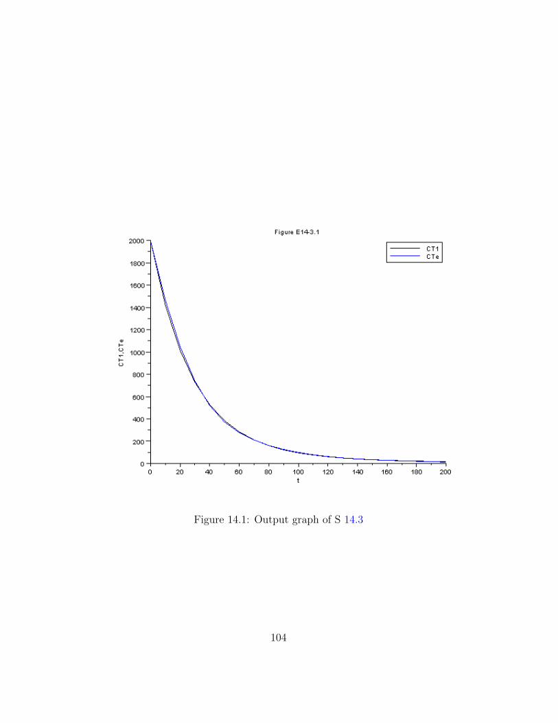
Figure 14.1: Output graph of S 14.3
104