Scilab Manual forDigital Signal Processingby Mr Vijay P SompurElectronics Engineering

Visvesvraya Technological University1

Solutions provided byMr. R.Senthilkumar- Assistant Professor

Electronics EngineeringInstitute of Road and Transport Technology

March 15, 2022

1Funded by a grant from the National Mission on Education through ICT,http://spoken-tutorial.org/NMEICT-Intro. This Scilab Manual and Scilab codeswritten in it can be downloaded from the ”Migrated Labs” section at the websitehttp://scilab.in

1

Contents

List of Scilab Solutions 4

1 Verification of Sampling theorem. 6

2 Impulse response of a given system 11

3 Linear Circular convolution of two given sequences 14

4 Autocorrelation of a given sequence and verification of itsproperties. 18

5 Cross correlation of given sequences and verification of itsproperties. 21

6 Solving a given difference equation. 24

7 Computation of N point DFT of a given sequence and toplot magnitude and phase spectrum. 26

8 Linear convolution of two sequences using DFT and IDFT. 30

9 Circular convolution of two given sequences using DFT andIDFT 33

10 Design and implementation of FIR filter to meet given spec-ifications. 35

11 Design and implementation of IIR filter to meet given spec-ifications. 39

2

12 Circular convolution of two given sequences 49

3

List of Experiments

Solution 1.1 Verification of Sampling Theorem . . . . . . . . . 6Solution 2.2 Program to find impulse response and Frequency

Response of a system . . . . . . . . . . . . . . . . 11Solution 3.1 Program to Compute the Convolution of Two Se-

quences . . . . . . . . . . . . . . . . . . . . . . . 14Solution 4.1 Program to Compute the Autocorrelation of a Se-

quence And verfication of Autocorrelation property 18Solution 5.1 Program to Compute the Crosscorrelation of a Se-

quence And verfication of crosscorrelation property 21Solution 6.1 Solving Difference Equation Direct Form II Real-

ization . . . . . . . . . . . . . . . . . . . . . . . . 24Solution 7.1 Program to find the spectral information of discrete

time signal Calculation of DFT and IDFT . . . . 26Solution 8.1 Linear Convolution using Circular Convolution DFT

IDFT method . . . . . . . . . . . . . . . . . . . . 30Solution 9.1 Circular Convolution using DFT IDFT method . 33Solution 10.1 To Design an Low Pass FIR Filter . . . . . . . . . 35Solution 11.1 To obtain Digital IIR Butterworth low pass filter

Frequency response . . . . . . . . . . . . . . . . . 39Solution 11.2 To obtain Digital IIR Chebyshev low pass filter Fre-

quency response . . . . . . . . . . . . . . . . . . . 43Solution 12.1 Program to perform circular convolution of two se-

quences . . . . . . . . . . . . . . . . . . . . . . . 49

4

List of Figures

1.1 Verification of Sampling Theorem . . . . . . . . . . . . . . . 91.2 Verification of Sampling Theorem . . . . . . . . . . . . . . . 10

2.1 Program to find impulse response and Frequency Response ofa system . . . . . . . . . . . . . . . . . . . . . . . . . . . . . 12

3.1 Program to Compute the Convolution of Two Sequences . . 15

7.1 Program to find the spectral information of discrete time signalCalculation of DFT and IDFT . . . . . . . . . . . . . . . . . 27

8.1 Linear Convolution using Circular Convolution DFT IDFTmethod . . . . . . . . . . . . . . . . . . . . . . . . . . . . . 31

10.1 To Design an Low Pass FIR Filter . . . . . . . . . . . . . . . 36

11.1 To obtain Digital IIR Butterworth low pass filter Frequencyresponse . . . . . . . . . . . . . . . . . . . . . . . . . . . . . 40

11.2 To obtain Digital IIR Chebyshev low pass filter Frequencyresponse . . . . . . . . . . . . . . . . . . . . . . . . . . . . . 44

5

Experiment: 1

Verification of Samplingtheorem.

Scilab code Solution 1.1 Verification of Sampling Theorem

1 // Capt ion : V e r i f i c a t i o n o f Sampl ing Theorem2 // [ 1 ] . Right Sampl ing [ 2 ] . Under Sampl ing [ 3 ] . Over

Sampl ing3 clc;

4 close;

5 clear;

6 fm=input( ’ Enter the input s i g n a l f r e qu en cy : ’ );7 k=input( ’ Enter the number o f Cyc l e s o f i nput s i g n a l :

’ );8 A=input( ’ Enter the ampl i tude o f i nput s i g n a l : ’ );9 tm =0:1/( fm*fm):k/fm;

10 x=A*cos(2* %pi*fm*tm);

11 figure (1);

12 a = gca();

13 a.x_location = ” o r i g i n ”;14 a.y_location = ” o r i g i n ”;15 plot(tm,x);

16 title( ’ORIGINAL SIGNAL ’ );17 xlabel( ’ Time ’ );

6

18 ylabel( ’ Amplitude ’ );19 xgrid (1)

20 // Sampl ing Rate ( Nyqu i s t Rate )=2∗fm21 fnyq =2*fm;

22 // UNDER SAMPLING23 fs =(3/4)*fnyq;

24 n=0:1/ fs:k/fm;

25 xn=A*cos (2* %pi*fm*n);

26 figure (2);

27 a = gca();

28 a.x_location = ” o r i g i n ”;29 a.y_location = ” o r i g i n ”;30 plot2d3( ’ gnn ’ ,n,xn);31 plot(n,xn, ’ r ’ );32 title( ’ Under Sampl ing ’ );33 xlabel( ’ Time ’ );34 ylabel( ’ Amplitude ’ );35 legend( ’ Sampled S i g n a l ’ , ’ Re con s t ru c t ed S i g n a l ’ );36 xgrid (1)

37 //NYQUIST SAMPLING38 fs=fnyq;

39 n=0:1/ fs:k/fm;

40 xn=A*cos (2* %pi*fm*n);

41 figure (3);

42 a = gca();

43 a.x_location = ” o r i g i n ”;44 a.y_location = ” o r i g i n ”;45 plot2d3( ’ gnn ’ ,n,xn);46 plot(n,xn, ’ r ’ );47 title( ’ Nyqu i s t Sampl ing ’ );48 xlabel( ’ Time ’ );49 ylabel( ’ Amplitude ’ );50 legend( ’ Sampled S i g n a l ’ , ’ Re con s t ru c t ed S i g n a l ’ );51 xgrid (1)

52 //OVER SAMPLING53 fs=fnyq *10;

54 n=0:1/ fs:k/fm;

55 xn=A*cos (2* %pi*fm*n);

7

56 figure (4);

57 a = gca();

58 a.x_location = ” o r i g i n ”;59 a.y_location = ” o r i g i n ”;60 plot2d3( ’ gnn ’ ,n,xn);61 plot(n,xn, ’ r ’ );62 title( ’ Over Sampl ing ’ );63 xlabel( ’ Time ’ );64 ylabel( ’ Amplitude ’ );65 legend( ’ Sampled S i g n a l ’ , ’ Re con s t ru c t ed S i g n a l ’ );66 xgrid (1)

67 // Re su l t68 // Enter the input s i g n a l f r e qu en cy : 1 0 069 //70 // Enter the number o f Cyc l e s o f i nput s i g n a l : 271 //72 // Enter the ampl i tude o f i nput s i g n a l : 2

8

Figure 1.1: Verification of Sampling Theorem

9

Figure 1.2: Verification of Sampling Theorem

10

Experiment: 2

Impulse response of a givensystem

Scilab code Solution 2.2 Program to find impulse response and FrequencyResponse of a system

1 // Capt ion : Program to f i n d impu l s e r e s p on s e and2 // Frequency Response o f a system3 //y [ n ] = a∗y [ n−1]+x [ n ]4 //Assume y [ n ] = h [ n ] , x [ n]= d e l t a [ n]= un i t impu l s e

r e s p on s e5 // a = 0 . 96 //h [ n ] = 0 . 9∗ h [ n−1]+ d e l t a [ n ]7 clc;

8 clear;

9 close;

10 a = 0.9; // c on s t an t a = 0 . 9 l e s s than 111 h0 = 1;

12 h1 = a; // f i r s t two v a l u e s o f impu l s e r e s p on s e13 h = [h0,h1,zeros (1 ,100)];

14 for i = 1:100

15 h(i+2) = ((a)^(i+1))*h(i+1);// impu l s e r e s p on s e

11

Figure 2.1: Program to find impulse response and Frequency Response of asystem

12

16 end

17 [HW ,W] = frmag(h,512); // f r e qu en cy r e s p on s e18 figure (1)

19 subplot (2,1,1)

20 a = gca();

21 a.x_location = ’ o r i g i n ’ ;22 a.y_location = ’ o r i g i n ’ ;23 plot ([1: length(h)],h, ’ r ’ );24 xlabel( ’ D i s c r e t e Time Index n−−−−> ’ );25 ylabel( ’ Impul se Response h [ n]−−−−−> ’ );26 title( ’ Impul se Response o f f i r s t o rd e r r e c u r s i v e

system ’ )27 xgrid (1)

28 subplot (2,1,2)

29 a = gca();

30 a.x_location = ’ o r i g i n ’ ;31 a.y_location = ’ o r i g i n ’ ;32 plot([ mtlb_fliplr (-2*%pi*W) ,2*%pi*W(2:$)],[

mtlb_fliplr(abs(HW)),abs(HW(2:$))])33 xlabel( ’ D i s c r e t e Frequency index W−−−−−−> ’ )34 ylabel( ’ Magnitude Response |H(W)|−−−−−−> ’ )35 title( ’ Frequency Response o f a cau sa l , s t a b l e , LTI

I s t Order Re cu r s i v e System ’ );36 xgrid (1)

13

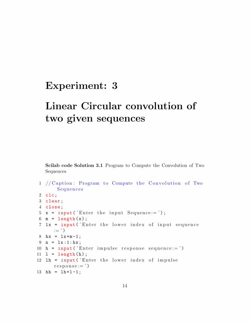
Experiment: 3

Linear Circular convolution oftwo given sequences

Scilab code Solution 3.1 Program to Compute the Convolution of TwoSequences

1 // Capt ion : Program to Compute the Convo lu t i on o f TwoSequence s

2 clc;

3 clear;

4 close;

5 x = input( ’ Enter the input Sequence := ’ );6 m = length(x);

7 lx = input( ’ Enter the l owe r index o f i nput s equence:= ’ )

8 hx = lx+m-1;

9 n = lx:1:hx;

10 h = input( ’ Enter impu l s e r e s p on s e s equence := ’ )11 l = length(h);

12 lh = input( ’ Enter the l owe r index o f impu l s er e s p on s e := ’ )

13 hh = lh+l-1;

14

Figure 3.1: Program to Compute the Convolution of Two Sequences

15

14 g = lh:1:hh;

15 nx = lx+lh;

16 nh = nx+m+l-2;

17 y = convol(x,h)

18 r = nx:nh;

19 figure (1)

20 subplot (3,1,1)

21 a = gca();

22 a.x_location = ” o r i g i n ”;23 a.y_location = ” o r i g i n ”;24 plot2d3( ’ gnn ’ ,n,x)25 xlabel( ’ n===> ’ )26 ylabel( ’ Amplitude−−> ’ )27 title( ’ Input Sequence x [ n ] ’ )28 subplot (3,1,2)

29 a = gca();

30 a.x_location = ” o r i g i n ”;31 a.y_location = ” o r i g i n ”;32 plot2d3( ’ gnn ’ ,g,h)33 xlabel( ’ n===> ’ )34 ylabel( ’ Amplitude−−−> ’ )35 title( ’ Impul se Response Sequence h [ n]= ’ )36 subplot (3,1,3)

37 a = gca();

38 a.x_location = ” o r i g i n ”;39 a.y_location = ” o r i g i n ”;40 plot2d3( ’ gnn ’ ,r,y)41 xlabel( ’ n===> ’ )42 ylabel( ’ Amplitude−−−> ’ )43 title( ’ Output Response Sequence y [ n]= ’ )44 //Example45 // Enter the input Sequence := [ 1 , 2 , 3 , 1 ]46 //47 // Enter the l owe r index o f i nput s equence :=048 //49 // Enter impu l s e r e s p on s e s equence := [1 , 2 , 1 , −1 ]50 //51 // Enter the l owe r index o f impu l s e r e s p on s e :=−1

16

52 //53 //54 //−−>y55 // y =56 //57 // 1 . 4 . 8 . 8 . 3 . − 2 . − 1 .58 //

17

Experiment: 4

Autocorrelation of a givensequence and verification of itsproperties.

Scilab code Solution 4.1 Program to Compute the Autocorrelation of aSequence And verfication of Autocorrelation property

1 // Capt ion : Program to Compute the Au t o c o r r e l a t i o n o fa Sequence

2 //And v e r f i c a t i o n o f Au t o c o r r e l a t i o n p r ope r t y3 clc;

4 clear;

5 close;

6 x = input( ’ Enter the input Sequence := ’ );7 m = length(x);

8 lx = input( ’ Enter the l owe r index o f i nput s equence:= ’ )

9 hx = lx+m-1;

10 n = lx:1:hx;

11 x_fold = x($:-1:1);12 nx = lx+lx;

13 nh = nx+m+m-2;

14 r = nx:nh;

18

15 Rxx = convol(x,x_fold);

16 disp(Rxx , ’ Auto C o r r e l a t i o n Rxx [ n ] := ’ )17 // Proper ty 1 : Au t o c o r r e l a t i o n o f a s equence has even

symmetry18 //Rxx [ n ] = Rxx[−n ]19 Rxx_flip = Rxx([$: -1:1]);20 if Rxx_flip ==Rxx then

21 disp( ’ P roper ty 1 : Auto Co r r e l a t i o n has EvenSymmetry ’ );

22 disp(Rxx_flip , ’ Auto C o r r e l a t i o n t ime r e v e r s e dRxx[−n ] := ’ );

23 end

24 // Proper ty 2 : Center va l u e Rxx [ 0 ]= t o t a l power o fthe s equence

25 Tot_Px = sum(x.^2);

26 Mid = ceil(length(Rxx)/2);

27 if Tot_Px == Rxx(Mid) then

28 disp( ’ P roper ty 2 : Rxx [ 0 ]= c e n t e r va l u e=max . va l u e=Tota l power o f i /p s equence ’ );

29 end

30 subplot (2,1,1)

31 plot2d3( ’ gnn ’ ,n,x)32 xlabel( ’ n===> ’ )33 ylabel( ’ Amplitude−−> ’ )34 title( ’ Input Sequence x [ n ] ’ )35 subplot (2,1,2)

36 plot2d3( ’ gnn ’ ,r,Rxx)37 xlabel( ’ n===> ’ )38 ylabel( ’ Amplitude−−> ’ )39 title( ’ Auto c o r r e l a t i o n Sequence Rxx [ n ] ’ )40 //Example41 // Enter the input Sequence := [ 2 , −1 , 3 , 4 , 1 ]42 //43 // Enter the l owe r index o f i nput s equence :=−244 //45 // Auto Co r r e l a t i o n Rxx [ n ] :=46 //47 // 2 . 7 . 5 . 1 1 . 3 1 . 1 1 . 5 .

19

7 . 2 .48 //49 // Proper ty 1 : Auto C o r r e l a t i o n has Even Symmetry50 //51 // Auto Co r r e l a t i o n t ime r e v e r s e d Rxx[−n ] :=52 //53 // 2 . 7 . 5 . 1 1 . 3 1 . 1 1 . 5 .

7 . 2 .54 //55 // Proper ty 2 : Rxx [ 0 ]= c e n t e r va l u e=max . va l u e=Tota l

power o f i /p s equence

20

Experiment: 5

Cross correlation of givensequences and verification of itsproperties.

Scilab code Solution 5.1 Program to Compute the Crosscorrelation of aSequence And verfication of crosscorrelation property

1 // Capt ion : Program to Compute the C r o s s c o r r e l a t i o no f a Sequence

2 //And v e r f i c a t i o n o f c r o s s c o r r e l a t i o n p r ope r t y3 clc;

4 clear;

5 close;

6 x = input( ’ Enter the F i r s t i nput Sequence := ’ );7 y = input( ’ Enter the second input Sequence := ’ )8 mx = length(x);

9 my = length(y);

10 lx = input( ’ Enter the l owe r index o f f i r s t i nputs equence := ’ )

11 ly = input( ’ Enter the l owe r index o f s econd inputs equence := ’ )

12 hx = lx+mx -1;

13 n = lx:1:hx;

21

14 x_fold = x($:-1:1);15 y_fold = y($:-1:1);16 nx = lx+ly;

17 ny = nx+mx+my -2;

18 r = nx:ny;

19 Rxy = convol(x,y_fold);

20 Ryx = convol(x_fold ,y);

21 disp(Rxy , ’ Cros s C o r r e l a t i o n Rxy [ n ] := ’ )22 count =1;

23 // Proper ty 1 : c r o s s c o r r e l a t i o n o f a s equence hasAntisymmetry

24 //Rxy [ n ] = Ryx[−n ]25 Ryx_flip = Ryx([$: -1:1]);26 for i = 1: length(Rxy)

27 if (ceil(Ryx_flip(i))==ceil(Rxy(i))) then

28 count = count +1;

29 end

30 end

31 if (count == length(Rxy)) then

32 disp( ’ P roper ty 1 : Cros s C o r r e l a t i o n hasAntiSymmetry : Rxy [ n]=Ryx[−n ] ’ );

33 end

34 // Proper ty 2 :% V e r i f i c a t i o n o f Energy Proper ty o fRxy

35 Ex = sum(x.^2);

36 Ey = sum(y.^2);

37 E = sqrt(Ex*Ey);

38 Mid = ceil(length(Rxy)/2);

39 if (E >= Rxy(Mid)) then

40 disp( ’ P roper ty 2 : Energy Proper ty o f Cros sC o r r e l a t i o n v e r i f i e d ’ )

41 end

42 subplot (2,1,1)

43 plot2d3( ’ gnn ’ ,n,x)44 xlabel( ’ n===> ’ )45 ylabel( ’ Amplitude−−> ’ )46 title( ’ Input Sequence x [ n ] ’ )47 subplot (2,1,2)

22

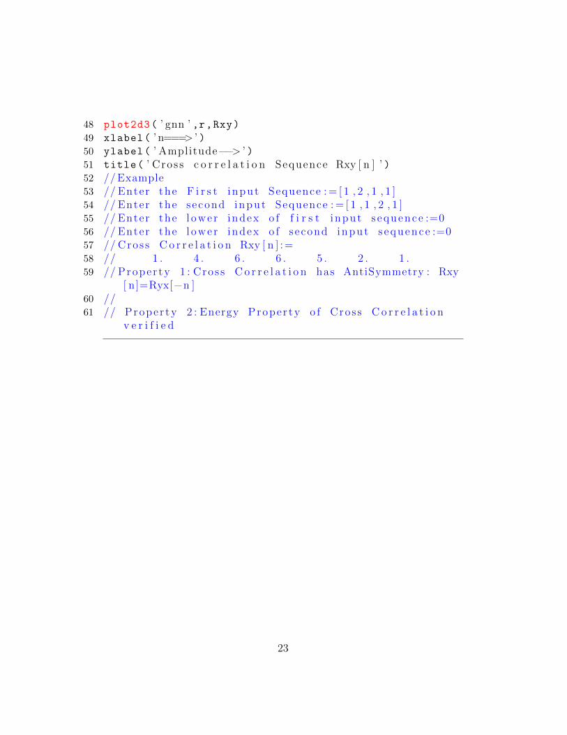
48 plot2d3( ’ gnn ’ ,r,Rxy)49 xlabel( ’ n===> ’ )50 ylabel( ’ Amplitude−−> ’ )51 title( ’ Cros s c o r r e l a t i o n Sequence Rxy [ n ] ’ )52 //Example53 // Enter the F i r s t i nput Sequence := [ 1 , 2 , 1 , 1 ]54 // Enter the second input Sequence := [ 1 , 1 , 2 , 1 ]55 // Enter the l owe r index o f f i r s t i nput s equence :=056 // Enter the l owe r index o f s econd input s equence :=057 // Cross C o r r e l a t i o n Rxy [ n ] :=58 // 1 . 4 . 6 . 6 . 5 . 2 . 1 .59 // Proper ty 1 : Cros s C o r r e l a t i o n has AntiSymmetry : Rxy

[ n]=Ryx[−n ]60 //61 // Proper ty 2 : Energy Proper ty o f Cros s C o r r e l a t i o n

v e r i f i e d

23

Experiment: 6

Solving a given differenceequation.

Scilab code Solution 6.1 Solving Difference Equation Direct Form II Re-alization

1 // Capt ion : S o l v i n g D i f f e r e n c e Equat ion2 // D i r e c t Form−I I R e a l i z a t i o n3 // F ind ing out the Output Response o f the f i r s t o r d e r4 // system ( F i l t e r )5 clc;

6 clear;

7 close;

8 x =

[1 ,1/2 ,1/4 ,1/8 ,1/16 ,1/32 ,1/64 ,1/128 ,1/256 ,1/512];

9 b = [3,-4/3]; // numerator po l ynom ia l s10 a = [1,-1/3]; // denominator po l ynom ia l s11 p = length(a) -1;

12 q = length(b) -1;

13 pq = max(p,q);

14 a = a(2:p+1);

15 w = zeros(1,pq);

16 for i = 1: length(x)

17 wnew = x(i)-sum(w(1:p).*a);

24

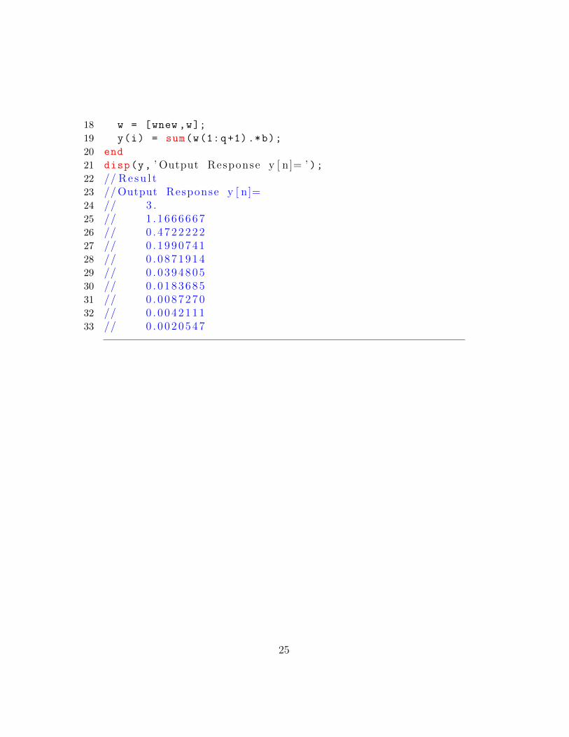
18 w = [wnew ,w];

19 y(i) = sum(w(1:q+1).*b);

20 end

21 disp(y, ’ Output Response y [ n]= ’ );22 // Re su l t23 //Output Response y [ n]=24 // 3 .25 // 1 . 166666726 // 0 . 472222227 // 0 . 199074128 // 0 . 087191429 // 0 . 039480530 // 0 . 018368531 // 0 . 008727032 // 0 . 004211133 // 0 . 0020547

25

Experiment: 7

Computation of N point DFTof a given sequence and to plotmagnitude and phase spectrum.

Scilab code Solution 7.1 Program to find the spectral information of dis-crete time signal Calculation of DFT and IDFT

1 // Capt ion : Program to f i n d the s p e c t r a l i n f o rma t i o no f d i s c r e t e t ime s i g n a l

2 // Ca l c u l a t i o n o f DFT and IDFT3 // P l o t t i n g Magnitude and Phase Spectrum4 clc;

5 close;

6 clear;

7 xn = input( ’ Enter the r e a l i nput d i s c r e t e s equence x[ n]= ’ );

8 N = length(xn);

9 XK = zeros(1,N);

10 IXK = zeros(1,N);

11 //Code b l o ck to f i n d the DFT o f the Sequence12 for K = 0:N-1

26

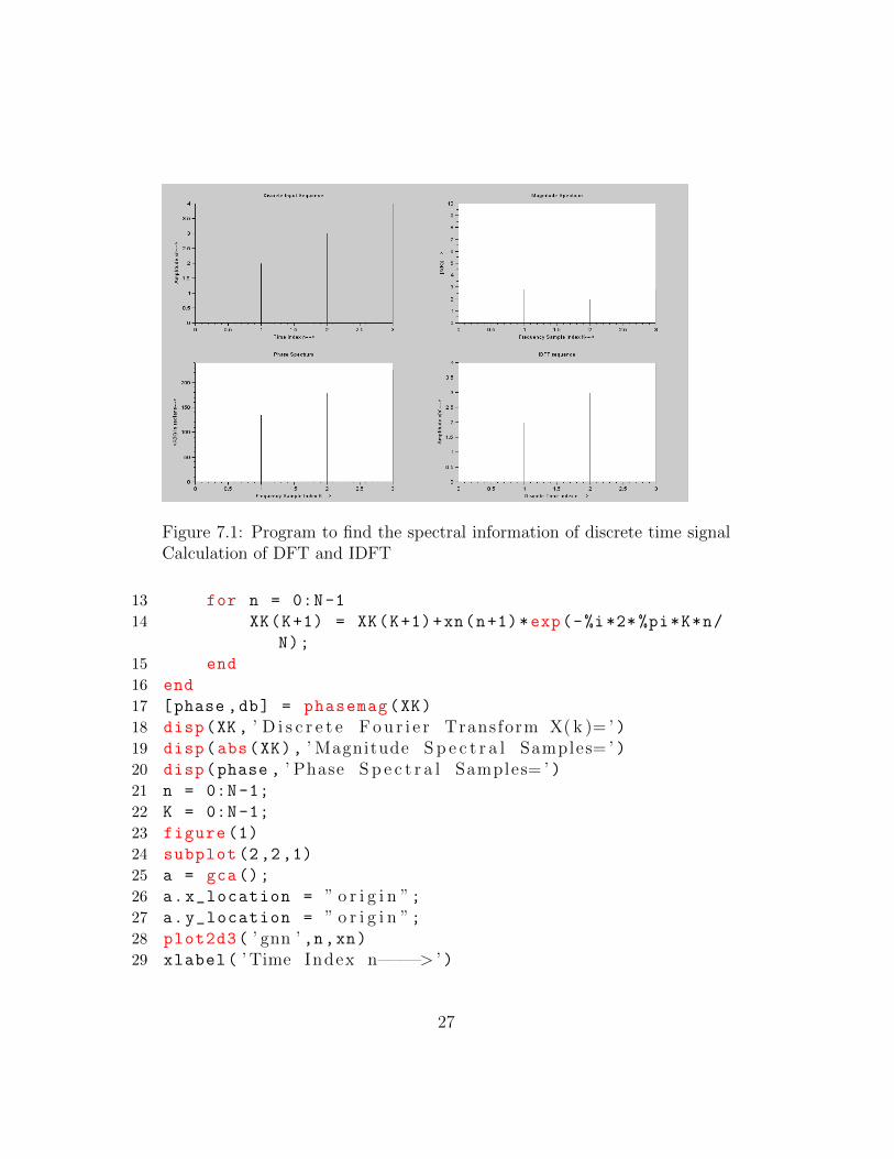
Figure 7.1: Program to find the spectral information of discrete time signalCalculation of DFT and IDFT

13 for n = 0:N-1

14 XK(K+1) = XK(K+1)+xn(n+1)*exp(-%i*2*%pi*K*n/

N);

15 end

16 end

17 [phase ,db] = phasemag(XK)

18 disp(XK, ’ D i s c r e t e Fou r i e r Transform X( k )= ’ )19 disp(abs(XK), ’ Magnitude S p e c t r a l Samples= ’ )20 disp(phase , ’ Phase S p e c t r a l Samples= ’ )21 n = 0:N-1;

22 K = 0:N-1;

23 figure (1)

24 subplot (2,2,1)

25 a = gca();

26 a.x_location = ” o r i g i n ”;27 a.y_location = ” o r i g i n ”;28 plot2d3( ’ gnn ’ ,n,xn)29 xlabel( ’ Time Index n−−−−> ’ )

27

30 ylabel( ’ Amplitude xn−−−−> ’ )31 title( ’ D i s c r e t e Input Sequence ’ )32 subplot (2,2,2)

33 a = gca();

34 a.x_location = ” o r i g i n ”;35 a.y_location = ” o r i g i n ”;36 plot2d3( ’ gnn ’ ,K,abs(XK))37 xlabel( ’ Frequency Sample Index K−−−−> ’ )38 ylabel( ’ |X(K) |−−−−> ’ )39 title( ’ Magnitude Spectrum ’ )40 subplot (2,2,3)

41 a = gca();

42 a.x_location = ” o r i g i n ”;43 a.y_location = ” o r i g i n ”;44 plot2d3( ’ gnn ’ ,K,phase)45 xlabel( ’ Frequency Sample Index K−−−−> ’ )46 ylabel( ’<X(K) in rad i an s−−−−> ’ )47 title( ’ Phase Spectrum ’ )48 //Code b l o ck to f i n d the IDFT o f the s equence49 for n = 0:N-1

50 for K = 0:N-1

51 IXK(n+1) = IXK(n+1)+XK(K+1)*exp(%i*2* %pi*K*n

/N);

52 end

53 end

54 IXK = IXK/N;

55 ixn = real(IXK);

56 subplot (2,2,4)

57 a = gca();

58 a.x_location = ” o r i g i n ”;59 a.y_location = ” o r i g i n ”;60 plot2d3( ’ gnn ’ ,[0:N-1],ixn)61 xlabel( ’ D i s c r e t e Time Index n −−−−> ’ )62 ylabel( ’ Amplitude x [ n]−−−−> ’ )63 title( ’ IDFT sequence ’ )64 //Example65 //66 // Enter the r e a l i nput d i s c r e t e s equence x [ n

28

] = [ 1 , 2 , 3 , 4 ]67 //68 // D i s c r e t e Fou r i e r Transform X( k )=69 //70 // 1 0 . − 2 . + 2 . i − 2 . − 9 . 7 97D−16 i − 2 . − 2 . i71 //72 // Magnitude S p e c t r a l Samples=73 //74 // 1 0 . 2 . 8284271 2 . 2 . 8 28427175 //76 // Phase S p e c t r a l Samples=77 //78 // 0 . 1 3 5 . 1 8 0 . 2 2 5 .79 //

29

Experiment: 8

Linear convolution of twosequences using DFT andIDFT.

Scilab code Solution 8.1 Linear Convolution using Circular ConvolutionDFT IDFT method

1 // Capt ion : L in ea r Convo lu t i on u s i n g C i r c u l a rConvo lu t i on

2 //DFT−IDFT method3 clc;

4 clear;

5 close;

6 x = input( ’ Enter the input d i s c r e t e s equence := ’ )7 h = input( ’ Enter the impu l s e d i s c r e t e s equence := ’ )8 N1 = length(x);

9 N2 = length(h);

10 N = N1+N2 -1; // L in ea r Convo lu t i on r e s u l t l e n g t h11 h = [h,zeros(1,N-N2)];

12 x = [x,zeros(1,N-N1)];

13 //Computing DFT−IDFT

30

Figure 8.1: Linear Convolution using Circular Convolution DFT IDFTmethod

31

14 XK = dft(x,-1);//N po i n t DFT o f i /p s equence15 HK = dft(h,-1);//N po i n t DFT o f impu l s e s equence16 // Mu l t i p l i c a t i o n o f 2 DFT’ s17 YK = XK.*HK;

18 // L in ea r Convo lu t i on r e s u l t19 yn = dft(YK ,1);//IDFT o f Y(K) ( o/p s equence )20 disp(real(yn), ’ L i n ea r Convo lu t i on r e s u l t y [ n ] := ’ )21 //Example22 // Enter the input d i s c r e t e s equence := [ 1 , 2 , 3 ]23 // Enter the impu l s e d i s c r e t e s equence := [ 1 , 2 , 2 , 1 ]24 // L in ea r Convo lu t i on r e s u l t y [ n ] :=25 //26 // 1 .27 // 4 .28 // 9 .29 // 1 1 .30 // 8 .31 // 3 .

32

Experiment: 9

Circular convolution of twogiven sequences using DFT andIDFT

Scilab code Solution 9.1 Circular Convolution using DFT IDFT method

1 // Capt ion : C i r c u l a r Convo lu t i on u s i n g DFT−IDFTmethod

2 clc;

3 clear;

4 close;

5 L = 4; // Length o f the s equence6 N = 4; //N−po i n t DFT7 x1 = input( ’ Enter the f i r s t d i s c r e t e s equence : x1 [ n]=

’ )8 x2 = input( ’ Enter the second d i s c r e t e s equence : x2 [ n

]= ’ )9 //Computing DFT10 X1K = dft(x1 ,-1);

11 X2K = dft(x2 ,-1);

12 // Mu l t i p l i c a t i o n o f 2 DFT’ s13 X3K = X1K.*X2K;

14 x3 = dft(X3K ,1); //IDFT o f X3(K)

33

15 x3 = real(x3);

16 disp(x3, ’ C i r c u l a r Convo lu t i on r e s u l t : x3 [ n]= ’ );17 //Example18 // Enter the f i r s t d i s c r e t e s equence : x1 [ n]= [ 2 , 1 , 2 , 1 ]19 // Enter the second d i s c r e t e s equence : x2 [ n]=

[ 1 , 2 , 3 , 4 ]20 //21 // C i r c u l a r Convo lu t i on r e s u l t : x3 [ n]=22 //23 // 1 4 .24 // 1 6 .25 // 1 4 .26 // 1 6 .

34

Experiment: 10

Design and implementation ofFIR filter to meet givenspecifications.

Scilab code Solution 10.1 To Design an Low Pass FIR Filter

1 // Capt ion : To Des ign an Low Pass FIR F i l t e r2 clc;

3 clear;

4 close;

5 wp= input( ’ Enter the pa s s band edge ( rad )= ’ );6 ws= input( ’ Enter the s t op band edge ( rad )= ’ );7 ks= input( ’ Enter the s t op band a t t e nu a t i o n (dB)= ’ );8 // I f 43<Ks<54 choo s e hamming window .9 //To s e l e c t N, o rd e r o f f i l t e r .10 N= (2* %pi*4)./(ws-wp); // k=4 f o r Hamming window .11 N= ceil(N); //To round−o f f N to the next i n t e g e r .12 wc=(wp+(ws-wp)/2)./%pi

13 // To ob ta i n FIR f i l t e r Impul se Response ’ wft ’14 //And FIR F i l t e r Frequency r e s p on s e ’wfm ’15 [wft ,wfm ,fr]=wfir( ’ l p ’ ,N+1,[wc/2,0], ’hm ’ ,[0,0]);

35

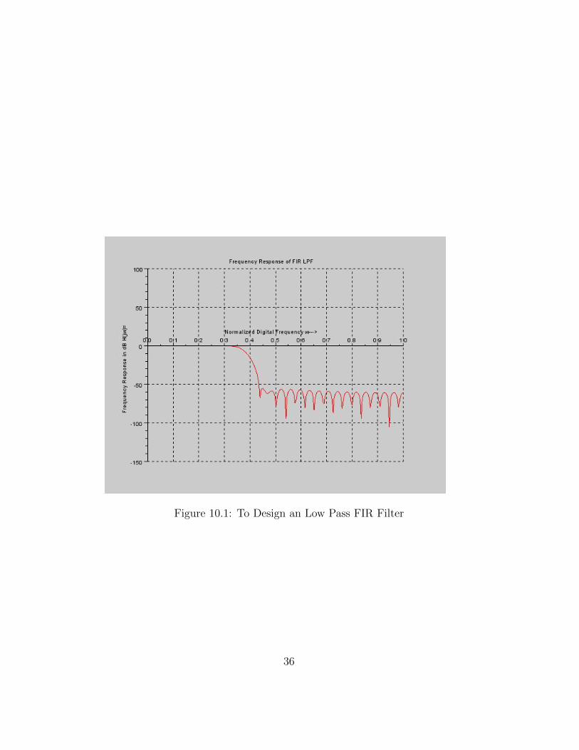
Figure 10.1: To Design an Low Pass FIR Filter

36

16 figure (1)

17 a = gca();

18 a.x_location = ” o r i g i n ”;19 a.y_location = ” o r i g i n ”;20 a.data_bounds = [0 , -150;1 ,50];

21 plot (2*fr ,20* log10(wfm), ’ r ’ )22 xlabel( ’ Normal i zed D i g i t a l Frequency w−−−> ’ )23 ylabel( ’ Frequency Response i n dB H( jw )= ’ )24 title( ’ Frequency Response o f FIR LPF ’ )25 xgrid (1)

26 // Re su l t27 // Enter the pa s s band edge ( rad )= 0 . 3∗%pi28 // Enter the s t op band edge ( rad )= 0 . 4 5∗%pi29 // Enter the s t op band a t t e nu a t i o n (dB)= 5030 //N = 54 .31 //−−>wc32 // wc = 0 . 3 7533 //−−>d i s p ( wft , ’ Impul se Response o f FIR LPF= ’)34 // Impul se Response o f FIR LPF=35 // column 1 to 736 // 0 . 0003609 − 0 . 0007195 − 0 . 0010869 1 . 5 7 5D

−18 0 . 0016485 0 . 0015927 − 0 . 001088337 // column 8 to 1438 // − 0 . 0035703 − 0 . 0017009 0 . 0038764

0 . 0061896 − 5 . 9 65D−18 − 0 . 0090208 − 0 . 008251639 // column 15 to 2140 // 0 . 0053105 0 . 0164428 0 . 0074408 −

0 . 0162551 − 0 . 0251602 1 . 1 9 1D−17 0 . 035948041 // column 22 to 2842 // 0 . 0334760 − 0 . 0225187 − 0 . 0756838 −

0 . 0394776 0 . 1111441 0 . 2931653 0 . 3 7 543 // column 29 to 3544 // 0 . 2931653 0 . 1111441 − 0 . 0394776 −

0 . 0756838 − 0 . 0225187 0 . 0334760 0 . 035948045 // column 36 to 4246 // 1 . 1 9 1D−17 − 0 . 0251602 − 0 . 0162551

0 . 0074408 0 . 0164428 0 . 0053105 − 0 . 008251647 // column 43 to 49

37

48 // − 0 . 0090208 − 5 . 9 65D−18 0 . 00618960 . 0038764 − 0 . 0017009 − 0 . 0035703 − 0 . 0010883column 50 to 55

49 // 0 . 0015927 0 . 0016485 1 . 5 7 5D−18 −0 . 0010869 − 0 . 0007195 0 . 0003609

38

Experiment: 11

Design and implementation ofIIR filter to meet givenspecifications.

Scilab code Solution 11.1 To obtain Digital IIR Butterworth low passfilter Frequency response

1 // Capt ion : To ob ta i n D i g i t a l I IR Butte rworth lowpas s f i l t e r

2 // Frequency r e s p on s e3 clc;

4 clear;

5 close;

6 fp= input( ’ Enter the pa s s band edge (Hz ) = ’ );7 fs= input( ’ Enter the s t op band edge (Hz ) = ’ );8 kp= input( ’ Enter the pa s s band a t t e nu a t i o n (dB) = ’ )

;

9 ks= input( ’ Enter the s t op band a t t e nu a t i o n (dB) = ’ );

10 Fs= input( ’ Enter the sampl ing r a t e sample s / s e c = ’ );

39

Figure 11.1: To obtain Digital IIR Butterworth low pass filter Frequencyresponse

40

11 d1 = 10^(kp/20);

12 d2 = 10^(ks/20);

13 d = sqrt ((1/(d2^2)) -1);

14 E = sqrt ((1/(d1^2)) -1);

15 // D i g i t a l f i l t e r s p e c i f i c a t i o n s ( rad / sample s )16 wp=2*%pi*fp*1/Fs;

17 ws=2*%pi*fs*1/Fs;

18 disp(wp, ’ D i g i t a l Pass band edge f r e q i n rad / sample swp= ’ )

19 disp(ws, ’ D i g i t a l Stop band edge f r e q i n rad / sample sws= ’ )

20 // Pre warping21 op=2*Fs*tan(wp/2);

22 os=2*Fs*tan(ws/2);

23 disp(op, ’ Analog Pass Band Edge Freq . i n rad / s e c op= ’)

24 disp(os, ’ Analog Stop band Edge Freq . i n rad / s e c os= ’)

25 N = log10(d/E)/log10(os/op);

26 oc = op/((E^2) ^(1/(2*N)));

27 N = ceil(N);// rounded to n e a r e s t i n t e g e r28 disp(N, ’ I IR F i l t e r o rd e r N = ’ );29 disp(oc, ’ Cu t o f f Frequency i n rad / s e cond s OC = ’ )30 [pols ,gn] = zpbutt(N,oc);

31 disp(gn, ’ Gain o f Analog IIR Butte rworth LPF Gain = ’ )32 disp(pols , ’ Po l e s o f Analog IIR Butte rworth LPF Po l e s

= ’ )33 HS = poly(gn, ’ s ’ , ’ c o e f f ’ )/real(poly(pols , ’ s ’ ));34 disp(HS, ’ T r an s f e r f u n c t i o n o f Ananlog IIR

Butte rworth LPF H(S )= ’ )35 z = poly(0, ’ z ’ )36 Hz = horner(HS ,(2*Fs*(z-1)/(z+1)))

37 num = coeff(Hz(2))

38 den = coeff(Hz(3))

39 Hz(2)= Hz(2)./den (3);

40 Hz(3) = Hz(3)./den(3);

41 disp(Hz, ’ T r an s f e r f u n c t i o n o f D i g i t l a IIRButte rworth LPF H(Z)= ’ )

41

42 [Hw ,w] = frmag(Hz ,256);

43 figure (1)

44 plot (2*w*%pi ,20* log10(abs(Hw)));

45 xlabel( ’ D i g i t a l Frequency w−−−> ’ )46 ylabel( ’ Magnitude i n dB 20 l o g |H(w) |= ’ )47 title( ’ Magnitude Response o f IIR LPF ’ )48 xgrid (1)

49 // Re su l t50 // Enter the pa s s band edge (Hz ) = 150051 //52 // Enter the s t op band edge (Hz ) = 200053 //54 // Enter the pa s s band a t t e nu a t i o n (dB) = −155 //56 // Enter the s t op band a t t e nu a t i o n (dB) = −357 //58 // Enter the sampl ing r a t e sample s / s e c = 800059 //60 // D i g i t a l Pass band edge f r e q i n rad / sample s wp=61 //62 // 1 . 178097263 //64 // D i g i t a l Stop band edge f r e q i n rad / sample s ws=65 //66 // 1 . 570796367 //68 // Analog Pass Band Edge Freq . i n rad / s e c op=69 //70 // 10690 . 85871 //72 // Analog Stop band Edge Freq . i n rad / s e c os=73 //74 // 16000 .75 //76 // IIR F i l t e r o rd e r N =77 //78 // 2 .79 //

42

80 // Cuto f f Frequency i n rad / s e cond s OC =81 //82 // 16022 . 76983 //84 // Gain o f Analog IIR Butte rworth LPF Gain =85 //86 // 2 . 5 6 7D+0887 //88 // Po l e s o f Analog IIR Butte rworth LPF Po l e s =89 //90 // − 11329 . 809 + 11329 . 809 i − 11329 . 809 −

11329 . 809 i91 //92 // T ran s f e r f u n c t i o n o f Ananlog IIR Butte rworth LPF

H(S )=93 //94 // 2 . 5 6 7D+0895 // −−−−−−−−−−−−−−−−−−−−−−−−−96 // 297 // 2 . 5 6 7D+08 + 22659 . 618 s + s98 //99 // T ran s f e r f u n c t i o n o f D i g i t l a IIR Butte rworth LPF

H(Z)=100 //101 // 2102 // 0 . 2933099 + 0 . 5866197 z + 0 . 2933099 z103 // −−−−−−−−−−−−−−−−−−−−−−−−−−−−−−−−−−−104 // 2105 // 0 . 1715734 + 0 . 0016661 z + z106 //

Scilab code Solution 11.2 To obtain Digital IIR Chebyshev low pass filterFrequency response

43

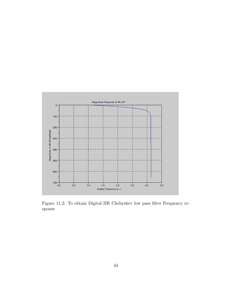
Figure 11.2: To obtain Digital IIR Chebyshev low pass filter Frequency re-sponse

44

1 // Capt ion : To ob ta i n D i g i t a l I IR Chebyshev low pas sf i l t e r

2 // Frequency r e s p on s e3 clc;

4 clear;

5 close;

6 fp= input( ’ Enter the pa s s band edge (Hz ) = ’ );7 fs= input( ’ Enter the s t op band edge (Hz ) = ’ );8 kp= input( ’ Enter the pa s s band a t t e nu a t i o n (dB) = ’ )

;

9 ks= input( ’ Enter the s t op band a t t e nu a t i o n (dB) = ’ );

10 Fs= input( ’ Enter the sampl ing r a t e sample s / s e c = ’ );

11 d1 = 10^(kp/20);

12 d2 = 10^(ks/20);

13 d = sqrt ((1/(d2^2)) -1);

14 E = sqrt ((1/(d1^2)) -1);

15 // D i g i t a l f i l t e r s p e c i f i c a t i o n s ( rad / sample s )16 wp=2*%pi*fp*1/Fs;

17 ws=2*%pi*fs*1/Fs;

18 disp(wp, ’ D i g i t a l Pass band edge f r e q i n rad / sample swp= ’ )

19 disp(ws, ’ D i g i t a l Stop band edge f r e q i n rad / sample sws= ’ )

20 // Pre warping21 op=2*Fs*tan(wp/2);

22 os=2*Fs*tan(ws/2);

23 disp(op, ’ Analog Pass Band Edge Freq . i n rad / s e c op= ’)

24 disp(os, ’ Analog Stop band Edge Freq . i n rad / s e c os= ’)

25 N = acosh(d/E)/acosh(os/op);

26 oc = op/((E^2) ^(1/(2*N)));

27 N = ceil(N);// rounded to n e a r e s t i n t e g e r28 disp(N, ’ I IR F i l t e r o rd e r N = ’ );29 disp(oc, ’ Cu t o f f Frequency i n rad / s e cond s OC = ’ )30 [pols ,gn] = zpch1(N,E,op);

45

31 disp(gn, ’ Gain o f Analog IIR Chebyshev Type−I LPFGain = ’ )

32 disp(pols , ’ Po l e s o f Analog IIR Chebyshev Type−I LPFPo l e s = ’ )

33 HS = poly(gn, ’ s ’ , ’ c o e f f ’ )/real(poly(pols , ’ s ’ ));34 disp(HS, ’ T r an s f e r f u n c t i o n o f Ananlog IIR Chebyshev

Type−I LPF H(S )= ’ )35 z = poly(0, ’ z ’ )36 Hz = horner(HS ,(2*Fs*(z-1)/(z+1)))

37 num = coeff(Hz(2))

38 den = coeff(Hz(3))

39 Hz(2)= Hz(2)./den (3);

40 Hz(3) = Hz(3)./den(3);

41 disp(Hz, ’ T r an s f e r f u n c t i o n o f D i g i t l a IIR ChebyshevLPF H(Z)= ’ )

42 [Hw ,w] = frmag(Hz ,256);

43 figure (1)

44 plot (2*w*%pi ,20* log10(abs(Hw)));

45 xlabel( ’ D i g i t a l Frequency w−−−> ’ )46 ylabel( ’ Magnitude i n dB 20 l o g |H(w) |= ’ )47 title( ’ Magnitude Response o f IIR LPF ’ )48 xgrid (1)

49 // Re su l t50 // Enter the pa s s band edge (Hz ) = 150051 //52 // Enter the s t op band edge (Hz ) = 200053 //54 // Enter the pa s s band a t t e nu a t i o n (dB) = −155 //56 // Enter the s t op band a t t e nu a t i o n (dB) = −357 //58 // Enter the sampl ing r a t e sample s / s e c = 800059 //60 // D i g i t a l Pass band edge f r e q i n rad / sample s wp=61 //62 // 1 . 178097263 //64 // D i g i t a l Stop band edge f r e q i n rad / sample s ws=

46

65 //66 // 1 . 570796367 //68 // Analog Pass Band Edge Freq . i n rad / s e c op=69 //70 // 10690 . 85871 //72 // Analog Stop band Edge Freq . i n rad / s e c os=73 //74 // 16000 .75 //76 // IIR F i l t e r o rd e r N =77 //78 // 2 .79 //80 // Cuto f f Frequency in rad / s e cond s OC =81 //82 // 17642 . 91283 //84 // Gain o f Analog IIR Chebyshev Type−I LPF Gain =85 //86 // 1 . 1 2 3D+0887 //88 // Po l e s o f Analog IIR Chebyshev Type−I LPF Po l e s =89 //90 // − 5867 . 861 + 9569 . 6927 i − 5867 . 861 − 9569 . 6927 i91 //92 // T ran s f e r f u n c t i o n o f Ananlog IIR Chebyshev Type−I

LPF H(S )=93 //94 // 1 . 1 2 3D+0895 // −−−−−−−−−−−−−−−−−−−−−−−−−96 // 297 // 1 . 2 6 0D+08 + 11735 . 722 s + s98 //99 // T ran s f e r f u n c t i o n o f D i g i t l a IIR Chebyshev LPF H(

Z)=100 //

47

101 // 2102 // 0 . 1971055 + 0 . 3942111 z + 0 . 1971055 z103 // −−−−−−−−−−−−−−−−−−−−−−−−−−−−−−−−−−−104 // 2105 // 0 . 3409008 − 0 . 4562766 z + z

48

Experiment: 12

Circular convolution of twogiven sequences

Scilab code Solution 12.1 Program to perform circular convolution of twosequences

1 // Capt ion : Program to per fo rm c i r c u l a r c o nv o l u t i o no f two s equ en c e s

2 clc;

3 clear;

4 close;

5 x1 = input( ’ Enter the f i r s t d i s c r e t e s equence := ’ )6 x2 = input( ’ Enter the second d i s c r e t e s equence := ’ )7 m = length(x1);// l e n g t h o f f i r s t s equence8 n = length(x2);// l e n g t h o f s econd s equence9 //To make l e n g t h o f x1 and x2 a r e equa l

10 if(m>n)

11 for i = n+1:m

12 x2(i)=0;

13 end

14 elseif(n>m)

15 for i = m+1:n

16 x1(i)=0;

17 end

49

18 end

19 N = length(x1);

20 x3 = zeros(1,N);// c i r c u l a r c o nv o l u t i o n r e s u l ti n i t i a l i z e d to z e r o

21 a(1) = x2(1);

22 for j = 2:N

23 a(j) = x2(N-j+2);

24 end

25 for i = 1:N

26 x3(1) = x3(1)+x1(i)*a(i);

27 end

28 X(1,:) = a;

29 // Ca l c u l a t i o n o f c i r c u l a r c o nv o l u t i o n30 for k =2:N

31 for j = 2:N

32 x2(j) = a(j-1);

33 end

34 x2(1) = a(N);

35 X(k,:) = x2;

36 for i = 1:N

37 a(i) = x2(i);

38 x3(k) = x3(k)+x1(i)*a(i);

39 end

40 end

41 disp(x3, ’ C i r c u l a r Convo lu t i on Re su l t x3 [ n]= ’ )42 //Example43 // Enter the f i r s t d i s c r e t e s equence := [ 2 , 1 , 2 , 1 ]44 // Enter the second d i s c r e t e s equence := [ 1 , 2 , 3 , 4 ]45 // C i r c u l a r Convo lu t i on Re su l t x3 [ n]=46 // 1 4 . 1 6 . 1 4 . 1 6 .47 //

50