Embed Size (px)
Citation preview

Scilab Textbook Companion forElectrical Engineering Fundamentals
by V. Del Toro1
Created byAditi Pohekar
Electrical EngineeringElectrical Engineering
IIT BombayCollege TeacherMadhu N. Belur
Cross-Checked byMukul R. Kulkarni
July 31, 2019
1Funded by a grant from the National Mission on Education through ICT,http://spoken-tutorial.org/NMEICT-Intro. This Textbook Companion and Scilabcodes written in it can be downloaded from the ”Textbook Companion Project”section at the website http://scilab.in

Book Description
Title: Electrical Engineering Fundamentals
Author: V. Del Toro
Publisher: Prentice - Hall International
Edition: 2
Year: 2009
ISBN: 9780132475525
1
Scilab numbering policy used in this document and the relation to theabove book.
Exa Example (Solved example)
Eqn Equation (Particular equation of the above book)
AP Appendix to Example(Scilab Code that is an Appednix to a particularExample of the above book)
For example, Exa 3.51 means solved example 3.51 of this book. Sec 2.3 meansa scilab code whose theory is explained in Section 2.3 of the book.
2

Contents
List of Scilab Codes 4
1 The Fundamental laws of Electrical Engineering 5
2 The circuit elements 6
3 Elementary network theory 13
4 Circuit differential equations Forms and Solutions 19
5 Circuit dynamics and forced responses 20
6 The laplace transform method of finding circuit solutions 22
7 Sinusoidal steady state response of circuits 23
9 Semiconductor electronic devices 31
11 Binary logic Theory and Implimentation 34
12 Simplifying logical functions 36
15 Magnetic circuit computations 37
16 Transformers 41
3
18 The three phase Induction motor 46
19 Computations of Synchronous Motor Performance 49
20 DC machines 51
23 Principles of Automatic Control 55
24 Dynamic behaviour of Control systems 56
4

List of Scilab Codes
Exa 1.1 force between two like charges in free space . 5Exa 2.1.a Determine the current flow and voltage drop
across the resistor . . . . . . . . . . . . . . . 6Exa 2.1.b Determine the current flow and voltage drop
across each resistor . . . . . . . . . . . . . . 6Exa 2.1.c Repeat parts A and B with the voltage source
replaced by a current source of 1A . . . . . 7Exa 2.2 From the given list of resistors choose a suit-
able resistor which can carry a current of 300mA 7Exa 2.3 Find the resistance of the round copper con-
ductor having the given specifications . . . . 8Exa 2.4 Find the resistance of the round copper con-
ductor having the given specifications . . . . 8Exa 2.5 Find the time variation of the voltage drop
appearing across the inductor terminals . . . 9Exa 2.6 Find the time variation of the capacitor volt-
age . . . . . . . . . . . . . . . . . . . . . . . 10Exa 2.7 Find A actual value of the voltage gain of
the opamp circuit B ideal value of the voltagegain C percent error . . . . . . . . . . . . . 10
Exa 2.8 Design a non inverting opamp circuit of volt-age gain 4 . . . . . . . . . . . . . . . . . . . 11
Exa 2.9 Find the input resistance of an inverting opampcircuit with voltage gain of 4 . . . . . . . . . 11
Exa 3.1 for the given circuit calculate the current flow-ing from the voltage source . . . . . . . . . 13
Exa 3.2 Calculate the potential difference across ter-minals bc . . . . . . . . . . . . . . . . . . . 13
5

Exa 3.3 Determine the equivalent series circuit . . . 14Exa 3.4 Value of E for which power dissipation in R5
is 15W R5 is 15 . . . . . . . . . . . . . . . . 14Exa 3.8 Find current flowing through all the branches
of the circuit . . . . . . . . . . . . . . . . . 16Exa 3.12 Find A current flowing through Rl B valye of
Rl for which the power transfer is maximumand the maximum power . . . . . . . . . . . 17
Exa 3.13 Find the current flowing through R2 by usingNortons current source equivalent circuit . . 18
Exa 4.3 Determine the operational driving point impedancesappearing at terminals ad and dg . . . . . . 19
Exa 5.2 Find the expression for the current flowingthrough the circuit and the total energy dis-sipated in the resistor . . . . . . . . . . . . 20
Exa 6.1 Find the laplace transform of the given pulse 22Exa 7.1 Find the average value of the given periodic
function . . . . . . . . . . . . . . . . . . . . 23Exa 7.2 Determine the power factor and average power
delivered to the circuit . . . . . . . . . . . . 23Exa 7.3 Find the expression for the sum of i1 and i2 24Exa 7.4 Find the effective value of the resultant current 24Exa 7.5 Find the time expression for the resultant cur-
rent . . . . . . . . . . . . . . . . . . . . . . 25Exa 7.6 Find the value of the given expression . . . 26Exa 7.7 Find A value of steady state current and the
relative phase angle C magnitude and phaseof voltage drops appearing across each ele-ment D average power E power factor . . . . 26
Exa 7.8 Find the equivalent impedance appearing be-tween points a and c . . . . . . . . . . . . . 28
Exa 7.9 Find the current which flows through branchZ3 . . . . . . . . . . . . . . . . . . . . . . . 28
Exa 7.10 Find the current in the Z3 branchby using theNodal method . . . . . . . . . . . . . . . . . 29
Exa 7.11 Find the current flowing through Z3 by usingThevinins theoram . . . . . . . . . . . . . . 30
6

Exa 9.2 Find the values of self bais source resistanceand drain load resistance at Q point . . . . 31
Exa 9.3 Find A midband frequency current gain of thefirst stage B bandwidth of the first stage am-plifier . . . . . . . . . . . . . . . . . . . . . 31
Exa 11.1 Determine th decimal equivalents of the bi-nary numbers A 101 B 11011 . . . . . . . . 34
Exa 11.2 Determine the decimal equivalent of A octalnumber 432 B hexadecimal number C4F . . 34
Exa 11.3 Find the binary and octal equivalents of 247 35Exa 15.1 Find A magneto motive force B current C rel-
ative permiability and reluctance of each ma-terial . . . . . . . . . . . . . . . . . . . . . . 37
Exa 15.3 Find the mmf produced by the coil . . . . . 38Exa 15.5 B Find the magnetic force exerted on the plunger 39Exa 16.1 Find A equivalent resistance and reactance
referred to both the sides B voltage dropsacross these in Volts and in per cent of therated winding voltage C Repeat B for the lowvoltage side D equivalent leakage impedancesreferred to both the sides . . . . . . . . . . . 41
Exa 16.2 Compute the 6 parameters of the equivalentcircuit referred to the high and low sides . . 43
Exa 16.3 For the transformer compute A efficiency Bvoltage regulation . . . . . . . . . . . . . . . 45
Exa 18.1 Find A input line current and power factorB developed electromagnetic torque C horsepower output D efficiency . . . . . . . . . . 46
Exa 19.1 Find A induced excitation voltage per phaseB line current C power factor . . . . . . . . 49
Exa 20.2 Caculate A electromagnetic torque B flux perpole C rotational losses D efficiency E shaftlaod . . . . . . . . . . . . . . . . . . . . . . 51
Exa 20.3 Determine the new operating speed . . . . . 52Exa 20.4 find A motor speed B required pulse frequency
C repeat part A and B for the given ON timeto cycle time ratio . . . . . . . . . . . . . . 53
7

Exa 23.1 Determine the new transfer gain and feedbackfactor . . . . . . . . . . . . . . . . . . . . . 55
Exa 24.2 find A dynamic response of the system B po-sition lag error C change in amplifier gain Ddamping ratio and maximum percent over-shoot E output gain factor for maximum over-shoot equal to 25percent . . . . . . . . . . . 56
8

Chapter 1
The Fundamental laws ofElectrical Engineering
Scilab code Exa 1.1 force between two like charges in free space
1 E0 = 1/(36* %pi *10^9); // p e r m i t i v i t y i n f r e e space2 k = 4*%pi*E0 ;
3 q1 = 1; // cha rge on the f i r s t p a r t i c l e i n coulombs4 q2 = 1; // cha rge on the second p a r t i c l e i n coulombs5 d = 1; // d i s t a n c e between the p a r t i c l e s i n meter6 F = (q1*q2)/(k*d^2); // f o r c e between the two
p a r t i c l e s i n newtons7
8 disp(F, ” f o r c e i n f r e e space between the twop a r t i c l e s i s i n Newtons i s : ”)
9

Chapter 2
The circuit elements
Scilab code Exa 2.1.a Determine the current flow and voltage drop across the resistor
1 V = 1; // v o l t a g e supp ly2 R = 10; // r e s i s t a n c e i n ohms3 I = V/R // c u r r e n t f l o w i n g through R4 disp(”a ) ”)5 disp(V,” v o l t a g e a c r o s s the r e s i s t o r ( i n v o l t s )=”)6 disp(I,” c u r r e n t f l o w i n g through the r e s i s t o r ( i n
amps ) =”)
Scilab code Exa 2.1.b Determine the current flow and voltage drop across each resistor
1 V = 1; // v o l t a g e supp ly2 R1 = 10; // f i r s t r e s i s t a n c e i n ohms3 R2 = 5; // r e s i s t a n c e o f the second r e s i s t o r4 Vr1 = V * (R1/(R1 + R2)); // v o l t a g e a c r o s s R15 Vr2 = V - Vr1; // v o l t a g e a c r o s s R26 Ir = Vr1/R1; // c u r r e n t f l o w i n g through R7
8 disp(Vr1 ,” v o l t a g e a c r o s s the f i r s t r e s i s t o r ( i nv o l t s )=”)
10

9 disp(Vr2 ,” v o l t a g e a c r o s s the second r e s i s t o r ( i nv o l t s )=”)
10 disp(Ir,” c u r r e n t f l o w i n g through the r e s i s t o r ( i namps ) =”)
Scilab code Exa 2.1.c Repeat parts A and B with the voltage source replaced by a current source of 1A
1 // c − a2 R1 = 10; // f i r s t r e s i s t a n c e i n ohms3 R2 = 5;
4 I = 1; // c u r r e n t s o u r c e5 V = I*R1; // v o l t a g e a c r o s s R6 disp(” c − a ) ”)7 disp(V,” v o l t a g e a c r o s s the r e s i s t o r ( i n v o l t s )=”)8 disp(I,” c u r r e n t f l o w i n g through the r e s i s t o r ( i n
amps ) =”)9
10 // c − b11 Vr1 = I*R1; // v o l t a g e a c r o s s R112 Vr2 = I*R2; // v o l t a g e a c r o s s R213 disp(” c − b ) ”)14 disp(V,” v o l t a g e a c r o s s the r e s i s t o r ( i n v o l t s )=”)15 disp(I,” c u r r e n t f l o w i n g through the r e s i s t o r ( i n
amps ) =”)
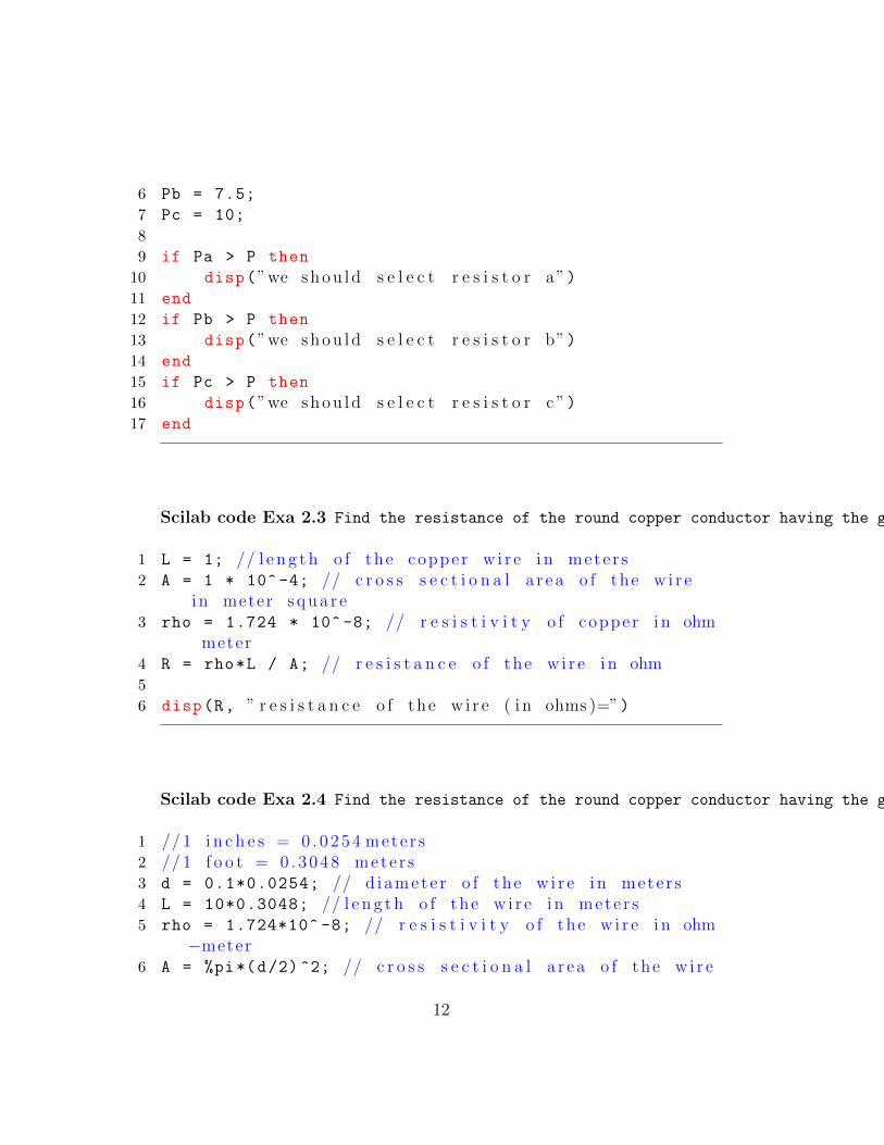
Scilab code Exa 2.2 From the given list of resistors choose a suitable resistor which can carry a current of 300mA
1 R = 100; // r e s i s t a n c e i n ohms2 I = 0.3; // c u r r e n t i n amps3 P = I^2 * R; // power4 // power s p e c i f i c a t i o n o f the r e s i s t o r s a v a i l a b l e i n
the s t o c k5 Pa = 5;
11
6 Pb = 7.5;
7 Pc = 10;
8
9 if Pa > P then
10 disp(”we shou ld s e l e c t r e s i s t o r a”)11 end
12 if Pb > P then
13 disp(”we shou ld s e l e c t r e s i s t o r b”)14 end
15 if Pc > P then
16 disp(”we shou ld s e l e c t r e s i s t o r c ”)17 end
Scilab code Exa 2.3 Find the resistance of the round copper conductor having the given specifications
1 L = 1; // l e n g t h o f the copper w i r e i n mete r s2 A = 1 * 10^-4; // c r o s s s e c t i o n a l a r ea o f the w i r e
i n meter squa r e3 rho = 1.724 * 10^ -8; // r e s i s t i v i t y o f copper i n ohm
meter4 R = rho*L / A; // r e s i s t a n c e o f the w i r e i n ohm5
6 disp(R, ” r e s i s t a n c e o f the w i r e ( i n ohms )=”)
Scilab code Exa 2.4 Find the resistance of the round copper conductor having the given specifications
1 // 1 i n c h e s = 0 . 0 2 5 4 meter s2 // 1 f o o t = 0 . 3 0 4 8 meter s3 d = 0.1*0.0254; // d iamete r o f the w i r e i n mete r s4 L = 10*0.3048; // l e n g t h o f the w i r e i n meter s5 rho = 1.724*10^ -8; // r e s i s t i v i t y o f the w i r e i n ohm
−meter6 A = %pi*(d/2) ^2; // c r o s s s e c t i o n a l a r ea o f the w i r e
12

7 R = rho*L/A; // r e s i s t a n c e o f the w i r e i n ohm8 disp(R,” r e s i s t a n c e o f the w i r e ( i n ohm)=”)
Scilab code Exa 2.5 Find the time variation of the voltage drop appearing across the inductor terminals
1 L = 0.1; // i n d u c t a n c e o f the c o i l i n henry2 t1 = [0:0.001:0.1];
3 t2 = [0.101:0.001:0.3];
4 t3 = [0.301:0.001:0.6];
5 t4 = [0.601:0.001:0.7];
6 t5 = [0.701:0.001:0.9]
7 // c u r r e n t v a r i a t i o n as a f u n c t i o n o f t ime8 i1 = 100*t1;
9 i2 = (-50*t2) + 15;
10 i3 = -100*sin(%pi*(t3 -0.3) /0.3);
11 i4 = (100*t4) - 60;
12 i5 = (-50*t5) + 45;
13
14 t = [t1 ,t2,t3,t4 ,t5];
15 i = [i1 ,i2,i3,i4 ,i5];
16 plot(t, i)
17
18 dt = 0.001;
19 di = diff(i);
20 V = L*di/dt; // v o l t a g e drop a p p ea r i n g a c r o s s thei n d u c t o r t e r m i n a l s
21 Tv = [0:0.001:0.899];
22 plot(Tv, V, ” g r e en ”)
13

Scilab code Exa 2.6 Find the time variation of the capacitor voltage
1 C = 0.01; // c a p a c i t a n c e o f the c a p a c i t o r i n Farads2 t1 = [0:0.001:0.1];
3 t2 = [0.101:0.001:0.3];
4 t3 = [0.301:0.001:0.6];
5 t4 = [0.601:0.001:0.7];
6 t5 = [0.701:0.001:0.9]
7 // c u r r e n t v a r i a t i o n as a f u n c t i o n o f t ime8 i1 = 100*t1;
9 i2 = (-50*t2) + 15;
10 i3 = -100*sin(%pi*(t3 -0.3) /0.3);
11 i4 = (100*t4) - 60;
12 i5 = (-50*t5) + 45;
13
14 t = [t1,t2,t3,t4 ,t5];
15 i = [i1,i2,i3,i4 ,i5];
16 plot(t, i)
17
18 // v o l t a g e a c r o s s the c a p a c i t o r as a f u n c t i o n o ft ime
19 V1 = (1/C)*integrate( ’ 100∗ t ’ , ’ t ’ ,0,t1);20 V2 = (1/C)*integrate( ’ (−50∗ t ) +15 ’ , ’ t ’ ,0.101,t2);21 V3 = (1/C)*integrate( ’ −100∗ s i n ( %pi ∗ ( t −0.3) / 0 . 3 ) ’ , ’ t ’
,0.301,t3);
22 V4 = (1/C)*integrate( ’ ( 100∗ t ) − 60 ’ , ’ t ’ ,0.601,t4);23 V5 = (1/C)*integrate( ’ (−50∗ t ) + 45 ’ , ’ t ’ ,0.701,t5);24 V = [V1 , V2 , V3, V4, V5];
25
26 plot(t, V, ” g r e en ”)
Scilab code Exa 2.7 Find A actual value of the voltage gain of the opamp circuit B ideal value of the voltage gain C percent error
1 // a2 Ri = 1;
14

3 Rf = 39;
4 A = 10^5; // open l oop ga in o f the op−amp5 G = A/(1 + (A*Ri/(Ri+Rf))); // a c t u a l v o l t a g e ga in o f
the c i r c u i t6 disp(”a”)7 disp(G,” a c t u a l v o l t a g e o f the c i r c u i t =”)8
9 //b10 G1 = 1 + (Rf/Ri); // v o l t a g e ga in o f the c i r c u i t
with i n f i n i t e open l oop ga in11 disp(”b”)12 disp(G1,” f o r i d e a l c a s e the v o l t a g e ga in =”)13
14 // c15 er = ((G1 - G)/G)*100; // p e r c e n t e r r o r16 disp(” c ”)17 disp(er,” p e r c e n t e r r o r o f the i d e a l v a l u e compared
to the a c t u a l v a l u e=”)
Scilab code Exa 2.8 Design a non inverting opamp circuit of voltage gain 4
1 G = 4; // v o l t a g e ga in o f the c i r c u i t2 r = G -1; // r a t i o o f the r e s i s t a n c e s i n the non−
i n v e r t i n g op−amp c i r c u i t3 disp(r,”Rf/ Ri =”)4 // R e s u l t :5 //A s u i t a b l e c h o i c e f o r R1 i s 10K, Hence Rf = 30K
Scilab code Exa 2.9 Find the input resistance of an inverting opamp circuit with voltage gain of 4
1 G = 4;
2 r = G; // r a t i o o f the r e s i s t a n c e s i n the i n v e r t i n gop−amp c i r c u i t
15

3 disp(r,”Rf/ Ri ”)4 // R e s u l t ;5 //A s u i t a b l e c h o i c e f o r Rf=30K and R1=7.5K6 // t h e r e f o r e input r e s i s t a n c e R1 = 7 . 5K
This code can be downloaded from the website wwww.scilab.in
16

Chapter 3
Elementary network theory
Scilab code Exa 3.1 for the given circuit calculate the current flowing from the voltage source
1 V = 100; // v o l a t a g e supp ly i n v o l t s2 Rs = 40; // r e s i s t a n c e i n s e r i e s i n ohms3 // p a r a l l e l r e s i s t a n c e s i n ohms4 Rp1 = 33.33;
5 Rp2 = 50;
6 Rp3 = 20;
7 Rpinv = (1/ Rp1)+(1/ Rp2)+(1/ Rp3); // r e c i p r o c a l o fe q u i v a l e n t r e s i s t a n c e i n p a r a l l e l
8 Req = Rs + (1/ Rpinv) ;
9 I = V/Req; // c u r r e n t f l o w i n g from the v o l t a g e s o u r c ei n amps
10 disp(I,” c u r r e n t f l o w i n g from the v o l t a g e s o u r c e ( i namps ) = ”)
Scilab code Exa 3.2 Calculate the potential difference across terminals bc
1 V = 100; // v o l a t a g e supp ly i n v o l t s2 Rs = 40; // r e s i s t a n c e i n s e r i e s i n ohms
17

3 // p a r a l l e l r e s i s t a n c e s i n ohms4 Rp1 = 33.33;
5 Rp2 = 50;
6 Rp3 = 20;
7 Rpinv = (1/ Rp1)+(1/ Rp2)+(1/ Rp3); // r e c i p r o c a l o fe q u i v a l e n t r e s i s t a n c e i n p a r a l l e l
8 Rp = 1/ Rpinv; // e q u i v a l e n t e s i s t a n c e i n p a r a l l e l9 Vbc = V*(Rp/(Rs + Rp)); // p o t e n t i a l d i f f e r e n c e
a c r o s s bc10 disp(Vbc ,” p o t e n t i a l d i f f e r e n c e a c r o s s bc = ”)
Scilab code Exa 3.3 Determine the equivalent series circuit
1 // r e s i s t a n c e s i n ohms2 R1 = 25;
3 R2 = 300;
4 R3 = 80;
5 R4 = 30;
6 R5 = 60;
7
8 Rcd = R5*R4/(R5 + R4);
9 Rbd1 = Rcd + R3;
10 Rbd = Rbd1*R2/(Rbd1 + R2);
11 Req = Rbd + R1; // e q u i v a l e n t r e s i s t a n c e12 disp(Req , ” e q u i v a l e n t r e s i s t a n c e = ”)
Scilab code Exa 3.4 Value of E for which power dissipation in R5 is 15W R5 is 15
1 // r e s i s t a n c e s i n ohms2 R1 = 25;
3 R2 = 300;
4 R3 = 80;
5 R4 = 30;
18

6 R5 = 60;
7
8 P5 = 15; // power d i s s i p a t e d i n R5 ( i n watt )9
10 I5 = sqrt(P5/R5); // c u r r e n t f l o w i n g through R511 V5 = R5*I5 ; // v o l t a g e a c r o s s R512 Vcd = V5; // v o l t a g e a c r o s s cd13
14 I4 = Vcd/R4; // c u r r e n t f l o w i n g through R415 Icd = I5 + I4; // c u r r e n t f l o w i n g through cd16
17 Vbd = (Icd*R3)+Vcd ; // v o l t a g e a c r o s s bd18 Ibd = (Vbd/R2)+Icd; // c u r r e n t through bd19
20 V1 = R1*Ibd; // v o l t a g e a c r o s s R121
22 E = V1 + Vbd;
23 disp(E,”E = ”)24
25 // R e s u l t : Value o f E f o r which power d i s s i p a t i o n i nR i s 15W = 200V
This code can be downloaded from the website wwww.scilab.in This
code can be downloaded from the website wwww.scilab.in This code can be
19
downloaded from the website wwww.scilab.in
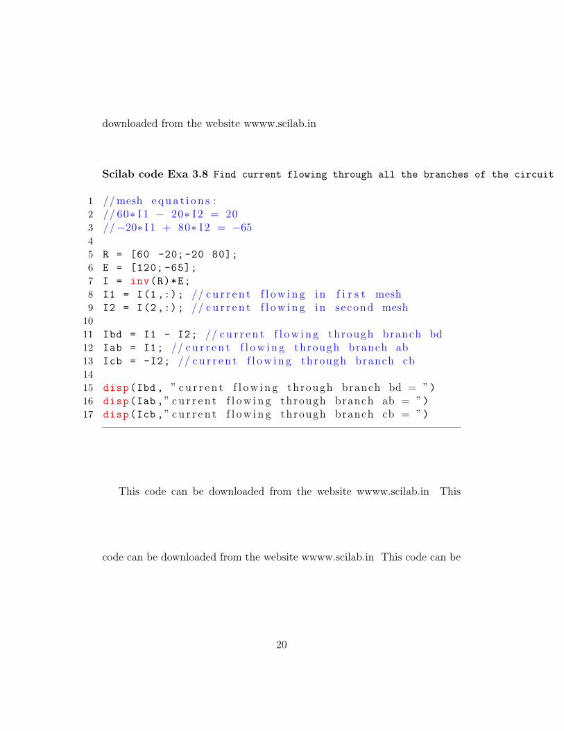
Scilab code Exa 3.8 Find current flowing through all the branches of the circuit
1 // mesh e q u a t i o n s :2 // 60∗ I 1 − 20∗ I 2 = 203 //−20∗ I 1 + 80∗ I 2 = −654
5 R = [60 -20;-20 80];
6 E = [120; -65];
7 I = inv(R)*E;
8 I1 = I(1,:); // c u r r e n t f l o w i n g i n f i r s t mesh9 I2 = I(2,:); // c u r r e n t f l o w i n g i n second mesh10
11 Ibd = I1 - I2; // c u r r e n t f l o w i n g through branch bd12 Iab = I1; // c u r r e n t f l o w i n g through branch ab13 Icb = -I2; // c u r r e n t f l o w i n g through branch cb14
15 disp(Ibd , ” c u r r e n t f l o w i n g through branch bd = ”)16 disp(Iab ,” c u r r e n t f l o w i n g through branch ab = ”)17 disp(Icb ,” c u r r e n t f l o w i n g through branch cb = ”)
This code can be downloaded from the website wwww.scilab.in This
code can be downloaded from the website wwww.scilab.in This code can be
20

downloaded from the website wwww.scilab.in
Scilab code Exa 3.12 Find A current flowing through Rl B valye of Rl for which the power transfer is maximum and the maximum power
1 // a2 // c i r c u i t pa ramete r s3 E1 = 120;
4 R1 = 40;
5 R2 = 20;
6 R3 = 60;
7
8 Voc = E1*R2/(R2 + R1); // open c i r c u i t v o l t a g ea p p ea r i n g at t e r m i n a l 1
9 Ri = R3 + (R1*R2/(R1 + R2)); // e q u i v a l e n t r e s i s t a n c el o o k i n g i n t o the network from t e r m i n a l p a i r
0110
11 function I = Il(Rl)
12 I = Voc/(Ri + Rl) // c u r r e n t through Rl13 endfunction
14
15 Il1 = Il(10); // Rl = 10 ohm16 Il2 = Il(50); // Rl = 50 ohm17 Il3 = Il(200); // Rl = 200 ohm18
19 disp(”a”)20 disp(Il1 ,” I l ( Rl = 10ohm) = ”)21 disp(Il2 ,” I l ( Rl = 50ohm) = ”)22 disp(Il3 ,” I l ( Rl = 200ohm) = ”)23
24 //b25 // f o r maximum power Rl = Ri26 Rl = Ri;
27 Plmax = (Voc /(2*Ri))^2 * Ri ; //maximum power to Rl28 disp(”b”)29 disp(Plmax ,”maximum power to Rl ( i n Watt ) = ”)
21

Scilab code Exa 3.13 Find the current flowing through R2 by using Nortons current source equivalent circuit
1 // c i r c u i t pa ramete r s2 // v o l t a g e s o u r c e s3 E1 = 120;
4 E2 = 65;
5 // r e s i s t a n c e s6 R1 = 40;
7 R2 = 11;
8 R3 = 60;
9
10 I = (E1/R1) + (E2/R3); // norton ’ s c u r r e n t s o u r c e11 Req = R1*R3/(R1 + R3); // e q u i v a l e n t r e s i s t a n c e12
13 I2 = I*Req/(Req + R2); // c u r r e n t f l o w i n g through R214
15 disp(I2,” c u r r e n t f l o w i n g through R2 = ”)
This code can be downloaded from the website wwww.scilab.in This code
can be downloaded from the website wwww.scilab.in
22

Chapter 4
Circuit differential equationsForms and Solutions
Scilab code Exa 4.3 Determine the operational driving point impedances appearing at terminals ad and dg
1 // ad2 Zab = complex (1,-0.5); // impedance a p p e a r i n g a c r o s s
t e r m i n a l s ab3 Zbg = complex (1); // impedance a p p e a r i n g a c r o s s
t e r m i n a l s bg4 Zbcd = complex (2+1 ,2); // impedance a p p e a r i n g a c r o s s
t e r m i n a l s bcd5 Zad = Zab + (Zbg*Zbcd/(Zbg + Zbcd)); // impedance
a p p ea r i n g a c r o s s t e r m i n a l s ad6 disp(Zad ,” impedance a pp e a r i n g a c r o s s t e r m i n a l s ad =
”)7
8 // dg9 Zdg = Zbg + (Zab*Zbcd/(Zab+Zbcd)); // impedance
a p p ea r i n g a c r o s s t e r m a i n a l s dg10 disp(Zdg ,” impedance a pp e a r i n g a c r o s s t e r m i n a l s dg =
”)
23

Chapter 5
Circuit dynamics and forcedresponses
This code can be downloaded from the website wwww.scilab.in
Scilab code Exa 5.2 Find the expression for the current flowing through the circuit and the total energy dissipated in the resistor
1 C = 10*10^ -6 ; // c a p a c i t a n c e ( i n f a r a d s )2 R = 0.2*10^6; // r e s i s t a n c e ( i n ohms )3 Vi = 40; // i n i t i a l v o l t a g e o f the c a p a c i t o r ( i n
v o l t s )4 Wc = (1/2)*C*Vi^2; // ene rgy s t o r e d i n the c a p a c i t o r5 // c u r r e n t f l o w i n g i n c i r c u i t as a f u n c t i o n o f t ime i
( t ) = 2∗10ˆ−4∗ exp(− t /2)6 // power d i s s i p a t e d i n the r e s i s t o r = R∗ i ˆ27 Wr = integrate( ’R∗4∗10ˆ−8∗ exp(− t ) ’ , ’ t ’ ,0,100)8 disp(Wc,” ene rgy s t o r e d i n the c a p a c i t o r ( i n J o u l e s ) =
”)
24

9 disp(Wr,” ene rgy d i s s i p a t e d i n the r e s i s t o r ( i n J o u l e s) = ”)
This code can be downloaded from the website wwww.scilab.in This
code can be downloaded from the website wwww.scilab.in This code can
be downloaded from the website wwww.scilab.in This code can be down-
loaded from the website wwww.scilab.in This code can be downloaded from
the website wwww.scilab.in This code can be downloaded from the website
wwww.scilab.in
25

Chapter 6
The laplace transform methodof finding circuit solutions
Scilab code Exa 6.1 Find the laplace transform of the given pulse
1 function F = laplace(s, T1, T2)
2 // p u l s e :3 // f = u ( t − T1) − u ( t − T2)4 F = integrate( ’ exp(− s ∗ t ) ’ , ’ t ’ ,T1 ,T2); // l a p l a c e
t r a n s f o r m o f the p u l s e5 endfunction
26

Chapter 7
Sinusoidal steady stateresponse of circuits
Scilab code Exa 7.1 Find the average value of the given periodic function
1 Vm = 2; // assumpt ion2 // ave rage v a l u e o f the f u n c t i o n3 //v ( t ) = Vm∗ a lpha /( %pi /3) f o r 0 <= alpha <= %pi /34 // = Vm f o r %pi /3 <= alpha <= %pi /25 Vav = (2/%pi)*integrate( ’Vm∗ a lpha ∗ (3/ %pi ) ’ , ’ a lpha ’
,0,%pi /3) + (2/%pi)*integrate( ’Vm∗ a lpha / a lpha ’ , ’a lpha ’ ,%pi/3,%pi /2);
6 disp(Vav)
Scilab code Exa 7.2 Determine the power factor and average power delivered to the circuit
1 theta = %pi /6; // phase d i f f e r e n c e between c u r r e n tand v o l t a g e
2 pf = cos(theta); // power f a c t o r3 disp(pf,” power f a c t o r = ”)4
27

5 Vm = 170; // peak v o l t a g e6 Im = 14.14; // peak c u r r e n t7
8 Pav = Vm*Im*pf/2; // ave rage power d e l i v e r e d to thec i r c u i t
9 disp(Pav ,” ave rage power d e l i v e r e d to the c i r c u i t = ”)
Scilab code Exa 7.3 Find the expression for the sum of i1 and i2
1 // l e t s assume tha t i 1 and i 2 a r e s t a t i o n a r y and thec o o r d i n a t e system i s r o t a t i n g with an a n g u l a r
f r q u e n c y o f w . And i 1 l i e s on the x−a x i s ( i . e .making an a n g l e o f 0 d e g r e e with the x−a x i s )
2 theta = %pi /3; // phase d i f f e r e n c e between i 1 and i 2 ;3 I1 = 10* sqrt (2); // peak v a l u e o f i 14 I2 = 20* sqrt (2); // peak v a l u e o f i 25 I = sqrt(I1^2 + I2^2 + 2*I1*I2*cos(theta)); // peak
v a l u e o f the r e s u l t a n t c u r r e n t6
7 phi = atan(I2*sin(theta)/(I1 + I2*cos(theta)));//phase d i f f e r e n c e between the r e s u l t a n t and i 1 ( i nr a d i a n s )
8 disp(I,” peak v a l u e o f the r e s u l t a n t c u r r e n t = ”)9 disp(phi ,” phase d i f f e r e n c e between the r e s u l t a n t and
i 1 = ”)10 // r e s u l t : i = I s i n ( wt + phi )
Scilab code Exa 7.4 Find the effective value of the resultant current
1 I1 = 10; // peak v a l u e o f i 12 I2 = 20; // peak v a l u e o f i 23 theta = %pi /3; // phase d i f f e r e n c e between i 1 and i 2
28
4 // complex r e p r e s e n t a t i o n o f the two c u r r e n t s5 i1 = complex (10);
6 i2 = complex (20* cos(%pi /3) ,20*sin(%pi/3));
7
8 i = i1 + i2 ; // r e s u l t a n t c u r r e n t9 I = sqrt (real(i)^2 + imag(i)^2); // c a l c u l a t i n g the
peak v a l u e o f the r e s u l t a n t c u r r e n t by u s i n g i t sr e a l and imag inary p a r t s
10 phi = atan(imag(i)/real(i)); // c a l c u l a t i g the phaseo f the r e s u l t a n t c u r r e n t by u s i n g i t s r e a l andimag inary p a r t s
11 disp(i,” r e s u l t a n t c u r r e n t = ”)12 disp(I,” peak v a l u e o f the r e s u l t a n t c u r r e n t = ”)13 disp(phi ,” phase o f the r e s u l t a n t c u r r e n t = ”)14 // r e s u l t : i = I s i n ( wt + phi )
Scilab code Exa 7.5 Find the time expression for the resultant current
1 I1 = 3; // peak v a l u e o f i 12 I2 = 5; // peak v a l u e o f i 23 I3 = 6; // peak v a l u e o f i 34 theta1 = %pi/6; // phase d i f f e r e n c e between i 2 and i 15 theta2 = -2*%pi /3; // phase d i f f e r e n c e between i 3 and
i 16 // complex r e p r e s e n t a t i o n o f the c u r r e n t s7 i1 = complex (3);
8 i2 = complex (5*cos(%pi /6) ,5*sin(%pi/6));
9 i3 = complex (6*cos(-2*%pi/3) ,6*sin(-2*%pi /3));
10
11 i = i1 + i2 + i3; // r e s u l t a n t c u r r e n t12 I = sqrt (real(i)^2 + imag(i)^2); // c a l c u l a t i n g the
peak v a l u e o f the r e s u l t a n t c u r r e n t by u s i n g i t sr e a l and imag inary p a r t s
13 phi = atan(imag(i)/real(i)); // c a l c u l a t i g the phaseo f the r e s u l t a n t c u r r e n t by u s i n g i t s r e a l and
29
imag ina ry p a r t s14 disp(I,” peak v a l u e o f the r e s u l t a n t c u r r e n t = ”)15 disp(phi ,” phase o f the r e s u l t a n t c u r r e n t = ”)16 // r e s u l t : i = I s i n ( wt + phi )
Scilab code Exa 7.6 Find the value of the given expression
1 // f i n d V∗Z1/Z22 V = complex (45* sqrt (3), -45);
3 Z1 = complex (2.5* sqrt (2), 2.5* sqrt (2));
4 Z2 = complex (7.5, 7.5* sqrt (3));
5 // we have to f i n d V∗Z1/Z26 Z = V*Z1/Z2;
7 disp(Z,”V∗Z1/Z2 = ”)
Scilab code Exa 7.7 Find A value of steady state current and the relative phase angle C magnitude and phase of voltage drops appearing across each element D average power E power factor
1 // a2 f = 60; // f r e q u e n c y o f the v o l a t g e s o u r c e3 V = complex (141);// v o l t a g e supp ly V = 141 s i n ( wt )4 R = 3; // r e s i s t a n c e o f the c i r c u i t5 L = 0.0106; // i n d u c t a n c e o f the c i r c u i t6 Z = complex(R,2*%pi*f*L);// impedance o f the c i r c u i t
= R + jwL7 i = V/Z; // c u r r e n t8 I = sqrt (real(i)^2 + imag(i)^2); // c a l c u l a t i n g the
peak v a l u e o f the c u r r e n t by u s i n g i t s r e a l andimag inary p a r t s
9 phi = atan(imag(i)/real(i)); // c a l c u l a t i g the phaseo f the r e s u l t a n t c u r r e n t by u s i n g i t s r e a l andimag inary p a r t s
10 disp(”a”)
30

11 disp(I,” e f f e c t i v e v a l u e o f the s t eady s t a t e c u r r e n t= ”)
12 disp(phi ,” r e l a t i v e phase a n g l e = ”)13
14 //b15 // e x p r e s s i o n f o r the i n s t a n t a n e o u s c u r r e n t can be
w r i t t e n as16 // i = I s i n ( wt + phi )17
18 // c19 R = complex (3);
20 vr = V*R/Z; // v o l t a g e a c r o s s the r e s i s t o r21 Vr = sqrt (real(vr)^2 + imag(vr)^2); // peak v a l u e o f
the v o l t a g e a c r o s s the r e s i s t o r22 phi1 = atan(imag(vr)/real(vr)); // phase o f the
v o l t a g e a c r o s s the r e s i s t o r23
24 vl = V - vr; // v o l t a g e a c r o s s the i n d u c t o r25 Vl = sqrt (real(vl)^2 + imag(vl)^2); // peak v a l u e o f
the v o l t a g e a c r o s s the i n d u c t o r26 phi2 = atan(imag(vl)/real(vl)); // phase o f the
v o l t a g e a c r o s s the i n d u c t o r27 disp(” c ”)28 disp(Vr,” e f f e c t i v e v a l u e o f the v o l t a g e drop a c r o s s
the r e s i s t o r = ”)29 disp(phi1 ,” phase o f the v o l t a g e drop a c r o s s the
r e s i s t o r = ”)30 disp(Vl,” e f f e c t i v e v a l u e o f the v o l t a g e drop a c r o s s
the i n d u c t o r = ”)31 disp(phi2 ,” phase o f the v o l t a g e drop a c r o s s the
i n d u c t o r = ”)32
33 //d34 Pav = V*I*cos(phi); // ave rage power d i s s i p a t e d by
the c i r c u i t35 disp(”d”)36 disp(Pav ,” ave rage power d i s s i p a t e d by the c i r c u i t =
”)
31

37
38 // e39 pf = cos(phi); // power f a c t o r40 disp(” e ”)41 disp(pf,” power f a c t o r = ”)
Scilab code Exa 7.8 Find the equivalent impedance appearing between points a and c
1 // impedances i n the c i r c u i t2 Z1 = complex (10 ,10);
3 Z2 = complex (15 ,20);
4 Z3 = complex (3,-4);
5 Z4 = complex (8,6);
6
7 Ybc = (1/Z2)+(1/Z3)+(1/Z4); // admit tance o f thep a r a l l e l combinat ion
8 Zbc = (1/Ybc); // impedance o f the p a r a l l e lcombinat i on
9
10 Z = Z1 + Zbc; // e q u i v a l e n t impedance o f the c i r c u i t11
12 disp(Z,” e q u i v a l e n t impedance o f the c i r c u i t = ”)
Scilab code Exa 7.9 Find the current which flows through branch Z3
1 V1 = complex (10);
2 V2 = complex (10* cos(-%pi/3) ,10*sin(-%pi/3));
3 Z1 = complex (1,1);
4 Z2 = complex (1,-1);
5 Z3 = complex (1,2);
6
7 // by mesh a n a l y s i s we g e t the f o l l o w i n g e q u a t i o n s :8 // I1 ∗Z11 − I 2 ∗Z12 = V1
32

9 //−I 1 ∗Z21 + I2 ∗Z22 = −V2 ; where I1 and I2 a r e thec u r r r e n t s f l o w i n g i n the f i r s t and second meshesr e s p e c t i v e l y
10 Z11 = Z1 + Z1;
11 Z12 = Z1 + Z2;
12 Z21 = Z12;
13 Z22 = Z2 + Z2;
14
15 // the mesh e q u a t i o n s can be r e p r e s e n t e d i n thematr ix form as I ∗Z = V
16 Z = [Z11 , -Z12; -Z21 , Z22]; // impedance matr ix17 V = [V1; -V2]; // v o l t a g e matr ix18 I = inv(Z)*V; // c u r r e n t matr ix = [ I1 ; I 2 ]19
20 I1 = I(1,:); // I1 = f i r s t row o f I matr ix21 I2 = I(2,:); // I1 = second row o f I matr ix22
23 Ibr = I1 - I2; // c u r r e n t f l o w i n g through Z324
25 disp(Ibr ,” c u r r e n t f l o w i n g through Z3 = ”)
Scilab code Exa 7.10 Find the current in the Z3 branchby using the Nodal method
1 V1 = complex (10);
2 V2 = complex (10* cos(-%pi/3) ,10*sin(-%pi/3));
3 Z1 = complex (1,1);
4 Z2 = complex (1,-1);
5 Z3 = complex (1,2);
6 //By a p p l i n g the noda l a n a l y s i s we g e t the f o l l o w i n ge q u a t i o n :
7 //Va ( ( 1 / Z1 ) +(1/Z2 ) +(1/Z3 ) ) = (V1/Z1 ) + (V2/Z2 )8
9 Y = (1/Z1)+(1/Z2)+(1/Z3);
10 Va = (1/Y)*((V1/Z1) + (V2/Z2)); // v o l t a g e o f node a11
33

12 Ibr = Va/Z3; // c u r r e n t f l o w i n g through Z313
14 disp(Ibr ,” c u r r e n t f l o w i n g through Z3 = ”)
Scilab code Exa 7.11 Find the current flowing through Z3 by using Thevinins theoram
1 V1 = complex (10);
2 V2 = complex (10* cos(-%pi/3) ,10*sin(-%pi/3));
3 Z1 = complex (1,1);
4 Z2 = complex (1,-1);
5 Z3 = complex (1,2);
6
7 Zth = Z3 + (Z1*Z2/(Z1+Z2)); // t h e v i n i n r e s i s t a n c e8
9 I = (V1 - V2)/(Z1 + Z2); // c u r r e n t f l o w i n g throughthe c i r c u i t when R3 i s not connec t ed
10 Vth = V1 - I*Z1; // t h e v i n i n v o l t a g e11
12 Ibr = Vth/Zth; // c u r r e n t f l o w i n g through Z313
14 disp(Ibr ,” c u r r e n t f l o w i n g through Z3 = ”)
34

Chapter 9
Semiconductor electronicdevices
Scilab code Exa 9.2 Find the values of self bais source resistance and drain load resistance at Q point
1 // Q u i e s c e n t p o i n t2 Idq = 0.0034; // d r a i n c u r r e n t3 Vdq = 15; // d r a i n v o l t a g e4 Vgq = 1; // ga t e v o l t a g e5
6 Vdd = 24; // d r a i n supp ly v o l t a g e7
8 Rs = Vgq/Idq;
9 disp(Rs,”The v a l u e o f s e l f b a i s s o u r c e r e s i s t a n c e i s( i n ohm) : ”)
10
11 Rd = (Vdd - Vdq)/Idq ;
12 disp(Rd,”The v a l u e o f d r a i n l oad r e s i s t a n c e i s ( i nohm) : ”)
Scilab code Exa 9.3 Find A midband frequency current gain of the first stage B bandwidth of the first stage amplifier
35

1 // a2 // t r a n s i s t o r pa ramete r s3 R2 = 0.625;
4 hie = 1.67;
5 Rb = 4.16;
6 Rl = 2.4;
7 Roe = 150;
8
9 Cc = 25 * 10^ -6;
10 rBB = 0.29;
11 rBE = 1.375;
12 Cd = 6900 * 10^ -12;
13 Ct = 40 * 10^ -12;
14 gm = 0.032;
15
16 Req = (Rl*Roe)/(Rl + Roe);
17 hfe = 44;
18 a = 1 + (R2/Req);
19 b = 1 + (hie/Rb);
20 Aim = -hfe/(a*b); // mid band f r e q u e n c y ga in21 disp(”a”)22 disp(Aim ,”The mid band f r e q u e n c y ga in o f the f i r s t
s t a g e o f the c i r c u i t i s : ”)23
24 //b25 Tl = 2*%pi*(Req + R2)*Cc *(10^3);
26 Fl = 1/Tl;
27
28 Rp = (Req*R2)/(Req + R2);
29 C = Cd + Ct*(1 + gm*Rp *10^3);
30 d = Rb + hie ;
31 e = rBE * (Rb + rBB)* 10^3 * C ;
32 Fh = d/(2* %pi*e);
33
34 BW = Fh - Fl;
35 disp(”b”)36 disp(BW, ”The bandwidth o f the f i r s t s t a g e
a m p l i f i e r i n Hz i s : ”)
36

37
Chapter 11
Binary logic Theory andImplimentation
Scilab code Exa 11.1 Determine th decimal equivalents of the binary numbers A 101 B 11011
1 // a2 N2 = ’ 101 ’ ; // b i n a r y o r d e r e d s equence3 N = bin2dec(N2); // dec ima l e q u i v a l e n t o f N24 disp(”a”)5 disp(N, ” dec ima l e q u i v a l e n t o f 101 = ”)6
7 //b8 N2 = ’ 11011 ’ ; // b i n a r y o r d e r e d s equence9 N = bin2dec(N2); // dec ima l e q u i v a l e n t o f N2
10 disp(”b”)11 disp(N, ” dec ima l e q u i v a l e n t o f 11011 = ”)
Scilab code Exa 11.2 Determine the decimal equivalent of A octal number 432 B hexadecimal number C4F
1 // a2 N8 = ’ 432 ’ ; // o c t a l number
38

3 N = oct2dec(N8); // dec ima l r e p r e s e n t a t i o n o f N84 disp(”a”)5 disp(N,” dec ima l e q u i v a l e n t o f 432 = ”)6
7 //b8 N16 = ’C4F ’ ; // hexadec ima l number9 N = hex2dec(N16); // dec ima l r e p r e s e n t a t i o n o f N1610 disp(”b”)11 disp(N,” dec ima l e q u i v a l e n t o f C4F = ”)
Scilab code Exa 11.3 Find the binary and octal equivalents of 247
1 N = 247;
2 N2 = dec2bin(N); // b i n a r y e q u i v a l e n t o f N3 N8 = dec2oct(N); // o c t a l e q u i v a l e n t o f N4 disp(N2, ” b in a r y e q u i v a l e n t o f 247 = ”)5 disp(N8, ” o c t a l e q u i v a l e n t o f 247 = ”)
39

Chapter 12
Simplifying logical functions
This code can be downloaded from the website wwww.scilab.in This code
can be downloaded from the website wwww.scilab.in This code can be down-
loaded from the website wwww.scilab.in
40
Chapter 15
Magnetic circuit computations
Scilab code Exa 15.1 Find A magneto motive force B current C relative permiability and reluctance of each material
1 // a2 phi = 6*10^ -4; // g i v e n magnet i c f l u x ( i n Wb)3 A = 0.001; // c r o s s s e c t i o n a l a r ea ( i n meter squa r e )4 B = phi/A ; //5 Ha = 10; // magnet i c f i e l d i n t e n s i t y o f m a t e r i a l a
needed to e s t a b l i s h the g i v e n magnet i c f l u x6 Hb = 77; // magnet i c f i e l d i n t e n s i t y o f m a t e r i a l b7 Hc = 270; // magnet i c f i e l d i n t e n s i t y o f m a t e r i a l c8 La = 0.3; // a r c l e n g t h o f m a t e r i a l a ( i n mete r s )9 Lb = 0.2; // a r c l e n g t h o f m a t e r i a l b ( i n meter s )
10 Lc = 0.1; // a r c l e n g t h o f m a t e r i a l c ( i n mete r s )11
12 F = Ha*La + Hb*Lb + Hc*Lc; // magnetomotive f o r c e13 disp(”a”)14 disp(F, ” magnetomotive f o r c e needed to e s t a b l i s h a
f l u x o f 6∗10ˆ−4( i n At ) = ”)15
16 //b17 N = 100; // no . o f t u r n s18 I = F/N; // c u r r e n t i n amps19 disp(”b”)
41

20 disp(I,” c u r r e n t tha t must be made to f l o w throughthe c o i l ( i n amps ) = ”)
21
22 // c23 MU0 = 4*%pi *10^ -7;
24 MUa = B/Ha; // p e r m e a b i l i t y o f m a t e r i a l a25 MUb = B/Hb; // p e r m e a b i l i t y o f m a t e r i a l b26 MUc = B/Hc; // p e r m e a b i l i t y o f m a t e r i a l c27
28 MUra = MUa/MU0; // r e l a t i v e p e r m e a b i l i t y o f m a t e r i a la
29 MUrb = MUb/MU0; // r e l a t i v e p e r m e a b i l i t y o f m a t e r i a lb
30 MUrc = MUc/MU0; // r e l a t i v e p e r m e a b i l i t y o f m a t e r i a lc
31
32 Ra = Ha*La/phi; // r e l u c t a n c e o f m a t e r i a l a33 Rb = Hb*Lb/phi; // r e l u c t a n c e o f m a t e r i a l b34 Rc = Hc*Lc/phi; // r e l u c t a n c e o f m a t e r i a l c35
36 disp(” c ”)37 disp(MUra ,” r e l a t i v e p e r m e a b i l i t y o f m a t e r i a l a = ”)38 disp(MUrb ,” r e l a t i v e p e r m e a b i l i t y o f m a t e r i a l b = ”)39 disp(MUrc ,” r e l a t i v e p e r m e a b i l i t y o f m a t e r i a l c = ”)40 disp(Ra,” r e l u c t a n c e o f m a t e r i a l a = ”)41 disp(Rb,” r e l u c t a n c e o f m a t e r i a l b = ”)42 disp(Rc,” r e l u c t a n c e o f m a t e r i a l c = ”)
Scilab code Exa 15.3 Find the mmf produced by the coil
1 mu0 = 4*%pi *10^ -7;
2 A = 0.0025; // c r o s s s e c t i o n a l a r ea o f the c o i l3 // d imens i on s o f the c o i l ( i n mete r s )4 Lg = 0.002; // a i r gap l e n g t h ( i n meter s )5 Lbd = 0.025;
42

6 Lde = 0.1;
7 Lef = 0.025;
8 Lfk = 0.2;
9 Lbc = 0.175;
10 Lcab = 0.5;
11
12 Lbghc = 2*( Lbd + Lde + Lef + (Lfk/2)) - Lg;// l e n g t ho f the f e r r o m a g n e t i c m a t e r i a l i n v o l v e d he r e
13
14 phig = 4*10^ -4; // a i r gap f l u x ( i n Wb)15 Bg = phig/A ; // a i r gap f l u x d e n s i t y ( i n t e s l a )16 Hg = Bg/mu0 ; // f e i l d i n t e n s i t y o f the a i r gap17 mmfg = Hg*Lg ; //mmf produced i n the a i r gap ( i n At )18
19 Bbc = 1.38 ; // f l u x d e n s i t y c o r r e s p o n d i n g to c a s ts t e e l
20
21 Hbghc = 125; // f i e l d i n t e n s i t y c o r r e s p o n d i n g to f l u xd e n s i t y o f 0 . 1 6T i n the s t e e l
22 mmfbghc = Hbghc*Lbghc ; // mmf c o r r e s p o n d i n g to bghc23
24 mmfbc = mmfg + mmfbghc ; //mmf a c r o s s path bc25 Hbc = mmfbc/Lbc;
26 phibc = Bbc*A ; // f l u x produced i n bc27
28 phicab = phig + phibc; // t o t a l f i u x e x i s t i n g i n l e gcab
29 Bcab = phicab /0.00375; // f l u x d e n s i t y30 Hcab = 690;
31 mmfcab = Hcab*Lcab; //mmf i n l e g cab32
33 mmf = mmfbc + mmfcab ; //mmf produced by the c o i l34
35 disp(mmf ,”mmf produced by the c o i l ( i n At ) = ”)
43

Scilab code Exa 15.5 B Find the magnetic force exerted on the plunger
1 //b2 mu0 = 4*%pi*10^-7 ;
3 // p l u n g e r magnet d imens i on s ( i n mete r s )4 x = 0.025;
5 h = 0.05;
6 a = 0.025;
7 g = 0.00125;
8
9 mmf = 1414; // ( i n At )10
11 F = %pi*a*mu0*(mmf^2)*(h^2) *(1/(x + h)^2)/g; //magnitude o f the f o r c e
12 disp(F, ” magnitude o f the f o r c e ( i n Newtons ) = ”)
44

Chapter 16
Transformers
Scilab code Exa 16.1 Find A equivalent resistance and reactance referred to both the sides B voltage drops across these in Volts and in per cent of the rated winding voltage C Repeat B for the low voltage side D equivalent leakage impedances referred to both the sides
1 // a2 V1 = 1100; // h i g h e r v o l t a g e3 V2 = 220; // l owe r v o l t a g e4 a = V1/V2; // t u r n s r a t i o5 r1 = 0.1; // h igh v o l t a g e wind ing r e s i s t a n c e ( i n ohms )6 x1 = 0.3; // h igh v o l t a g e l e a k a g e r e a c t a n c e ( i n ohms )7 r2 = 0.004; // low v o l t a g e wind ing r e s i s t a n c e ( i n ohms
)8 x2 = 0.012; // low v o l t a g e l e a k a g e r e a c t a n c e ( i n ohms )9
10 Re1 = r1 + (a^2)*r2 ; // e q u i v a l e n t wind ingr e s i s t a n c e r e f e r r e d to the pr imary s i d e
11 Xe1 = x1 + (a^2)*x2 ; // e q u i v a l e n t l e a k a g e r e a c t a n c er e f e r r e d to the pr imary s i d e
12 Re2 = (r1/a^2) + r2 ; // e q u i v a l e n t wind ingr e s i s t a n c e r e f e r r e d to the s e condary s i d e
13 Xe2 = (x1/a^2) + x2 ; // e q u i v a l e n t l e a k a g e r e a c t a n c er e f e r r e d to the s e condary s i d e
14
15 disp(”a”)16 disp(Re1 ,” e q u i v a l e n t wind ing r e s i s t a n c e r e f e r r e d to
45

the pr imary s i d e ”)17 disp(Xe1 ,” e q u i v a l e n t l e a k a g e r e a c t a n c e r e f e r r e d to
the pr imary s i d e ”)18 disp(Re2 ,” e q u i v a l e n t wind ing r e s i s t a n c e r e f e r r e d to
the s e conda ry s i d e ”)19 disp(Xe2 ,” e q u i v a l e n t l e a k a g e r e a c t a n c e r e f e r r e d to
the s e conda ry s i d e ”)20
21 //b22 P = 100; // power ( i n kVA)23 I21 = P*1000/ V1; // pr imary wind ing c u r r e n t r a t i n g24 Vre1 = I21*Re1; // e q u i v a l e n t r e s i s t a n c e drop ( i n
v o l t s )25 VperR1 = Vre1 *100/V1 ; // % e q u i v a l e n t r e s i s t a n c e
drop26
27 Vxe1 = I21*Xe1; // e q u i v a l e n t r e a c t a n c e drop ( i nv o l t s )
28 VperX1 = Vxe1 *100/V1; // % e q u i v a l e n t r e a c t a n c e drop29
30 disp(”b”)31 disp(Vre1 ,” e q u i v a l e n t r e s i s t a n c e drop e x p r e s s e d i n
terms o f pr imary q u a n t i t i e s ( i n v o l t s ) = ”)32 disp(VperR1 ,”% e q u i v a l e n t r e s i s t a n c e drop e x p r e s s e d
i n terms o f pr imary q u a n t i t i e s = ”)33 disp(Vxe1 ,” e q u i v a l e n t r e a c t a n c e drop e x p r e s s e d i n
terms o f pr imary q u a n t i t i e s ( i n v o l t s ) =”)34 disp(VperX1 ,”% e q u i v a l e n t r e a c t a n c e drop e x p r e s s e d
i n terms o f pr imary q u a n t i t i e s = ”)35
36 // c37 I2 = a*I21; // s e conda ry winding c u r r e n t r a t i n g38 Vre2 = I2*Re2; // e q u i v a l e n t r e s i s t a n c e drop ( i n
v o l t s )39 VperR2 = Vre2 *100/V2 ; // % e q u i v a l e n t r e s i s t a n c e
drop40
41 Vxe2 = I2*Xe2; // e q u i v a l e n t r e a c t a n c e drop ( i n v o l t s
46

)42 VperX2 = Vxe2 *100/V2; // % e q u i v a l e n t r e a c t a n c e drop43
44 disp(” c ”)45 disp(Vre2 ,” e q u i v a l e n t r e s i s t a n c e drop e x p r e s s e d i n
terms o f s e conda ry q u a n t i t i e s ( i n v o l t s ) = ”)46 disp(VperR2 ,”% e q u i v a l e n t r e s i s t a n c e drop e x p r e s s e d
i n terms o f s e condary q u a n t i t i e s = ”)47 disp(Vxe2 ,” e q u i v a l e n t r e a c t a n c e drop e x p r e s s e d i n
terms o f s e conda ry q u a n t i t i e s ( i n v o l t s ) =”)48 disp(VperX2 ,”% e q u i v a l e n t r e a c t a n c e drop e x p r e s s e d
i n terms o f s e condary q u a n t i t i e s = ”)49
50 //d51 Ze1 = complex(Re1 ,Xe1); // e q u i v a l e n t l e a k a g e
impedance r e f e r r e d to the pr imary52 Ze2 = Ze1/a ; // e q u i v a l e n t l e a k a g e impedance
r e f e r r e d to the s e conda ry53
54 disp(”d”)55 disp(Ze1 ,” e q u i v a l e n t l e a k a g e impedance r e f e r r e d to
the pr imary = ”)56 disp(Ze2 ,” e q u i v a l e n t l e a k a g e impedance r e f e r r e d to
the s e condary = ”)
Scilab code Exa 16.2 Compute the 6 parameters of the equivalent circuit referred to the high and low sides
1 Pl = 396; // wattmeter r e a d i n g on open c i r c u i t t e s t2 Vl = 120; // v o l t m e t e r r e a d i n g on open c i r c u i t t e s t3 Il = 9.65; // ammeter r e a d i n g o open c i r c u i t t e s t4 a = 2400/120; // t u r n s r a t i o5
6 theata = acos(Pl/(Vl*Il)); // phase d i f f e r e n c ebetween v o l t a g e and c u r r e n t
7 Irl = Il*cos(theata); // r e s i s t i v e pa r t o f Im
47

8 Ixl = Il*sin(theata); // r e a c t i v e pa r t o f Im9
10 rl = Vl/Irl; // low v o l t a g e wind ing r e s i s t a n c e11 rh = (a^2)*rl; // r l on the h igh s i d e12 xl = Vl/Ixl; // magne t i z i ng r e a c t a n c e r e f e r r e d to the
l owe r s i d e13 xh = (a^2)*xl; // c o r r e s p o n d i n g h igh s i d e v a l u e14
15 Ph = 810; // wattmeter r e a d i n g on s h o r t c i r c u i t t e s t16 Vh = 92; // v o l t m e t e r r e a d i n g on s h o r t c i r c u i t t e s t17 Ih = 20.8; // ammeter r e a d i n g on s h o r t c i r c u i t t e s t18
19 Zeh = Vh/Ih; // e q u i v a l e n t impeadance r e f e r r e d to theh i g h e r s i d e
20 Zel = Zeh/(a^2); // e q u i v a l e n t impedance r e f e r r e d tothe l owe r s i d e
21 Reh = Ph/(Ih^2); // e q u i v a l e n t r e s i s t a n c e r e f e r r e d tothe h i g h e r s i d e
22 Rel = Reh/(a^2); // e q u i v a l e n t r e s i s t a n c e r e f e r r e d tothe l owe r s i d e
23 Xeh = sqrt((Zeh ^2) - (Reh^2)); // e q u i v a l e n tr e a c t a n c e r e f e r r e d to the h i g h e r s i d e
24 Xel = Xeh/(a^2); // e q u i v a l e n t r e a c t a n c e r e f e r r e d tothe l owe r s i d e
25
26 disp(Zeh ,” e q u i v a l e n t impeadance r e f e r r e d to theh i g h e r s i d e = ”)
27 disp(Zel ,” e q u i v a l e n t impedance r e f e r r e d to the l owe rs i d e = ”)
28 disp(Reh ,” e q u i v a l e n t r e s i s t a n c e r e f e r r e d to theh i g h e r s i d e = ”)
29 disp(Rel ,” e q u i v a l e n t r e s i s t a n c e r e f e r r e d to thel owe r s i d e = ”)
30 disp(Xeh ,” e q u i v a l e n t r e a c t a n c e r e f e r r e d to theh i g h e r s i d e = ”)
31 disp(Xel ,” e q u i v a l e n t r e a c t a n c e r e f e r r e d to the l owe rs i d e = ”)
48
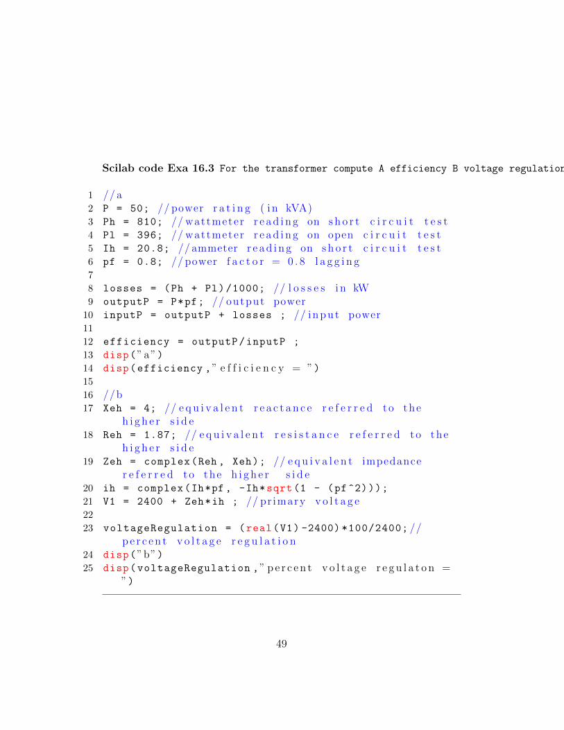
Scilab code Exa 16.3 For the transformer compute A efficiency B voltage regulation
1 // a2 P = 50; // power r a t i n g ( i n kVA)3 Ph = 810; // wattmeter r e a d i n g on s h o r t c i r c u i t t e s t4 Pl = 396; // wattmeter r e a d i n g on open c i r c u i t t e s t5 Ih = 20.8; // ammeter r e a d i n g on s h o r t c i r c u i t t e s t6 pf = 0.8; // power f a c t o r = 0 . 8 l a g g i n g7
8 losses = (Ph + Pl)/1000; // l o s s e s i n kW9 outputP = P*pf; // output power
10 inputP = outputP + losses ; // input power11
12 efficiency = outputP/inputP ;
13 disp(”a”)14 disp(efficiency ,” e f f i c i e n c y = ”)15
16 //b17 Xeh = 4; // e q u i v a l e n t r e a c t a n c e r e f e r r e d to the
h i g h e r s i d e18 Reh = 1.87; // e q u i v a l e n t r e s i s t a n c e r e f e r r e d to the
h i g h e r s i d e19 Zeh = complex(Reh , Xeh); // e q u i v a l e n t impedance
r e f e r r e d to the h i g h e r s i d e20 ih = complex(Ih*pf, -Ih*sqrt(1 - (pf^2)));
21 V1 = 2400 + Zeh*ih ; // pr imary v o l t a g e22
23 voltageRegulation = (real(V1) -2400) *100/2400; //p e r c e n t v o l t a g e r e g u l a t i o n
24 disp(”b”)25 disp(voltageRegulation ,” p e r c e n t v o l t a g e r e g u l a t o n =
”)
49

Chapter 18
The three phase Inductionmotor
Scilab code Exa 18.1 Find A input line current and power factor B developed electromagnetic torque C horse power output D efficiency
1 // a2 V1 = 440/ sqrt (3);
3 s = 0.025; // s l i p4 r1 = 0.1;
5 r2 = 0.12;
6 x1 = 0.35;
7 x2 = 0.4;
8
9 z = complex(r1 + r2/s, x1 + x2);
10 i2 = V1/z; // input l i n e c u r r e n t11 I2 = sqrt(real(i2)^2 + imag(i2)^2); // magnitude o f
i nput l i n e c u r r e n t12 disp(”a”)13 disp(i2,” input l i n e c u r r e n t = ”)14
15 i1 = complex (18* cos ( -1.484), 18*sin ( -1.484)); //magne t i z i ng c u r r e n t
16 I1 = sqrt(real(i1)^2 + imag(i1)^2); // magnitude o fmagne t i z i ng c u r r e n t
50
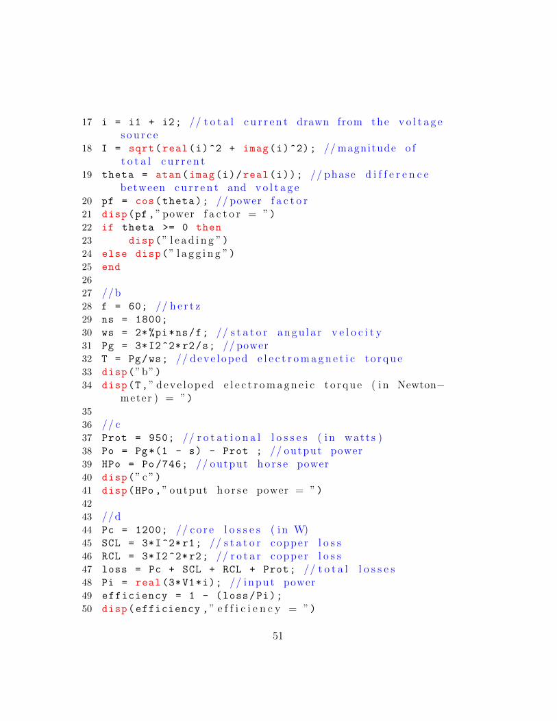
17 i = i1 + i2; // t o t a l c u r r e n t drawn from the v o l t a g es o u r c e
18 I = sqrt(real(i)^2 + imag(i)^2); // magnitude o ft o t a l c u r r e n t
19 theta = atan(imag(i)/real(i)); // phase d i f f e r e n c ebetween c u r r e n t and v o l t a g e
20 pf = cos(theta); // power f a c t o r21 disp(pf,” power f a c t o r = ”)22 if theta >= 0 then
23 disp(” l e a d i n g ”)24 else disp(” l a g g i n g ”)25 end
26
27 //b28 f = 60; // h e r t z29 ns = 1800;
30 ws = 2*%pi*ns/f; // s t a t o r a n g u l a r v e l o c i t y31 Pg = 3*I2^2*r2/s; // power32 T = Pg/ws; // deve l oped e l e c t r o m a g n e t i c t o r q ue33 disp(”b”)34 disp(T,” deve l oped e l e c t r o m a g n e i c t o rq u e ( i n Newton−
meter ) = ”)35
36 // c37 Prot = 950; // r o t a t i o n a l l o s s e s ( i n watt s )38 Po = Pg*(1 - s) - Prot ; // output power39 HPo = Po/746; // output h o r s e power40 disp(” c ”)41 disp(HPo ,” output h o r s e power = ”)42
43 //d44 Pc = 1200; // c o r e l o s s e s ( i n W)45 SCL = 3*I^2*r1; // s t a t o r copper l o s s46 RCL = 3*I2^2*r2; // r o t a r copper l o s s47 loss = Pc + SCL + RCL + Prot; // t o t a l l o s s e s48 Pi = real (3*V1*i); // input power49 efficiency = 1 - (loss/Pi);
50 disp(efficiency ,” e f f i c i e n c y = ”)
51

52

Chapter 19
Computations of SynchronousMotor Performance
Scilab code Exa 19.1 Find A induced excitation voltage per phase B line current C power factor
1 // a2 efficiency = 0.9;
3 Pi = 200*746/ efficiency; // input power4 x = 11; // r e a c t a n c e o f the motor5 V1 = 2300/ sqrt (3); // v o l t a g e r a t i n g6 delta = 15* %pi /180; // power a n g l e7 Ef = Pi*x/(3*V1*sin(delta)); // the induced
e x c i t a t i o n v o l t a g e per phase8 disp(”a”)9 disp(Ef,” the induced e x c i t a t i o n v o l t a g e per phase =
”)10
11 //b12 z = complex(0,x); // impedance o f the motor13 ef = complex(Ef*cos(-delta),Ef*sin(-delta));
14
15 Ia = (V1 - ef)/z ; // armature c u r r e n t16 disp(”b”)17 disp(Ia,” armatur c u r r e n t = ”)
53

18
19 // c20 theata = atan(imag(Ia)/real(Ia)); // phase d i f f e r e n c e
between Ia and V121 pf = cos(theata); // power f a c t o r22
23 disp(” c ”)24 disp(pf,” power f a c t o r = ”)25
26 if sin(theata)> 0 then
27 disp(” l e a d i n g ”)28 else
29 disp(” l a g g i n g ”)30 end
54

Chapter 20
DC machines
Scilab code Exa 20.2 Caculate A electromagnetic torque B flux per pole C rotational losses D efficiency E shaft laod
1 // a2 Vt = 230; // ( i n v o l t s )3 Ia = 73; // armature c u r r e n t ( i n amps )4 If = 1.6; // f e i l d c u r r e n t ( i n amps )5 Ra = 0.188; // armature c i r c u i t r e s i s t a n c e ( i n ohms )6 n = 1150; // r a t e d speed o f the r o t o r ( i n rpm )7 Po = 20*746; // output power ( i n watt s )8
9 Ea = Vt - (Ia*Ra); // armature v o l t a g e10 wm = 2*%pi*n/60; // r a t e d speed o f the r o t o r ( i n rad /
s e c )11 T = Ea*Ia/wm ; // e l e c t r o m a g n e t i c t o r q ue12
13 disp(”a”)14 disp(T,” e l e c t r o m a g n e t i c t o r q u e = ”)15
16 //b17 a = 4; // no . o f p a r a l l e l armature paths18 p = 4; // no . o f p o l e s19 z = 882; // no . o f armature c o n d u c t o r s20 flux = Ea*60*a/(p*z*n); // f l u x per p o l e ( i n Wb)
55
21
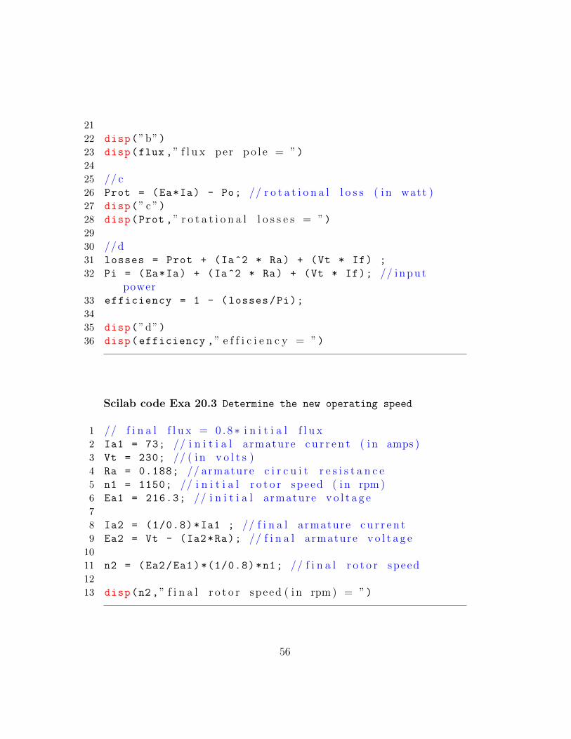
22 disp(”b”)23 disp(flux ,” f l u x per p o l e = ”)24
25 // c26 Prot = (Ea*Ia) - Po; // r o t a t i o n a l l o s s ( i n watt )27 disp(” c ”)28 disp(Prot ,” r o t a t i o n a l l o s s e s = ”)29
30 //d31 losses = Prot + (Ia^2 * Ra) + (Vt * If) ;
32 Pi = (Ea*Ia) + (Ia^2 * Ra) + (Vt * If); // inputpower
33 efficiency = 1 - (losses/Pi);
34
35 disp(”d”)36 disp(efficiency ,” e f f i c i e n c y = ”)
Scilab code Exa 20.3 Determine the new operating speed
1 // f i n a l f l u x = 0 . 8∗ i n i t i a l f l u x2 Ia1 = 73; // i n i t i a l armature c u r r e n t ( i n amps )3 Vt = 230; // ( i n v o l t s )4 Ra = 0.188; // armature c i r c u i t r e s i s t a n c e5 n1 = 1150; // i n i t i a l r o t o r speed ( i n rpm )6 Ea1 = 216.3; // i n i t i a l armature v o l t a g e7
8 Ia2 = (1/0.8)*Ia1 ; // f i n a l armature c u r r e n t9 Ea2 = Vt - (Ia2*Ra); // f i n a l armature v o l t a g e
10
11 n2 = (Ea2/Ea1)*(1/0.8)*n1; // f i n a l r o t o r speed12
13 disp(n2,” f i n a l r o t o r speed ( i n rpm ) = ”)
56

Scilab code Exa 20.4 find A motor speed B required pulse frequency C repeat part A and B for the given ON time to cycle time ratio
1 // a2 rop = 0.4; // r a t i o o f ON time T0 to c y c l e t ime Tp3 Vb =550; // r a t e d t e r m i n a l v o l t a g e o f the dc motor4 Ia = 30; // c u r r e n t drawn by the motor ( i n amps )5 Ra = 1; // armature c i r c u i t r e s i s t a n c e ( i n ohms )6 ts = 5.94; // t o r q u e and speed parameter o f the motor
( i n N−m/A)7
8 Vm = rop*Vb; // ave rage v a l u e o f the armaturet e r m i n a l v o l t a g e
9 Ea = Vm - (Ia*Ra); // induced armature v o l t a g e10
11 wm = Ea/ts; // motor speed ( i n rad / s )12 disp(”a”)13 disp(wm,” motor speed ( i n rad / s ) = ”)14
15 //b16 deltaI = 5; // change o f armature c u r r e n t dur ing the
ON p e r i o d17 La = 0.1; // armature wind ing i n d u c t a n c e ( i n H)18 To = La*deltaI /(Vb - Ea); //ON time19 Tp = To/rop; // c y c l e t ime20
21 f = 1/Tp ; // r e q u i r e d p u l s e s per second22 disp(”b”)23 disp(f,” r e q u i r e d p u l s e s per second = ”)24
25 // c26 rop = 0.7; //new r a t i o o f ON time T0 to c y c l e t ime
Tp27 Vm = rop*Vb; // ave rage v a l u e o f the armature
t e r m i n a l v o l t a g e
57
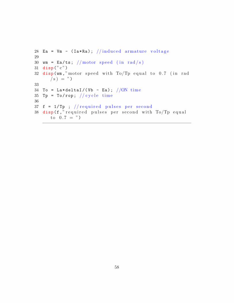
28 Ea = Vm - (Ia*Ra); // induced armature v o l t a g e29
30 wm = Ea/ts; // motor speed ( i n rad / s )31 disp(” c ”)32 disp(wm,” motor speed with To/Tp e q u a l to 0 . 7 ( i n rad
/ s ) = ”)33
34 To = La*deltaI /(Vb - Ea); //ON time35 Tp = To/rop; // c y c l e t ime36
37 f = 1/Tp ; // r e q u i r e d p u l s e s per second38 disp(f,” r e q u i r e d p u l s e s per second with To/Tp e q u a l
to 0 . 7 = ”)
58

Chapter 23
Principles of AutomaticControl
Scilab code Exa 23.1 Determine the new transfer gain and feedback factor
1 deltaGi = 420 - 380; // v a r i a t i o n i n the wi thoutf e e d b a c k ga in
2 Gi = 400; // wi thout f e e d b a c k ga in3 T = 400; // t r a n s f e r f u n c t i o n o f the c l o s e d l oop
system4 // ( v a r i a t i o n i n T) /T = ( change i n G) /G ∗ (1/ 1+H∗G)
= 0 . 0 25 // 1 + H∗G = R6 R = (deltaGi/Gi)/0.02;
7
8 G = T*R; //new d i r e c t t r a n s m i s s i o n ga in withf e e d b a c k
9 H = (G/T - 1)/G; // f e e d b a c k f a c t o r10
11 disp(G,”new d i r e c t t r a n s m i s s i o n ga in with f e e d b a c k =”)
12 disp(H,” f e e d b a c k f a c t o r s = ”)
59

Chapter 24
Dynamic behaviour of Controlsystems
Scilab code Exa 24.2 find A dynamic response of the system B position lag error C change in amplifier gain D damping ratio and maximum percent overshoot E output gain factor for maximum overshoot equal to 25percent
1 // a2 // parameter v a l u e s3 Kp = 0.5; //V/ rad4 Ka = 100; //V/V5 Km = 2*10^ -4 ; // lb− f t /V6 F = 1.5*10^ -4; // lb− f t / rad / s7 J = 10^-5 // s lug− f t ˆ28
9 K = Kp*Ka*Km ; // l oop p r o p o t i o n a l ga in10 dr = F/(2* sqrt(K*J)); // damping r a t i o11 wn = sqrt(K/J);
12 ts = 5/(dr*wn);
13 wd = wn*sqrt(1 - dr^2); // f r e q u e n c y at which dampedo s c i l l a t i o n s oc cu r
14 disp(”a”)15 disp(wd, ”damped o s c i l l a t i o n s oc cu r at a f r e q u e n c y =
”)16 disp(dr,” damping r a t i o = ”)17
60

18 //b19 Tl = 10^-3; // l oad d i s t u r b a n c e ( lb− f t )20 e = Tl/K; // p o s i t i o n l a g e r r o r21 disp(”b”)22 disp(e,” p o s i t i o n l a g e r r o r ( i n rad ) = ”)23
24 // c25 KaNew = (e/0.025)*Ka; //new loop ga in26 disp(” c ”)27 disp(KaNew ,”new loop ga in f o r which the p o s i t i o n l a g
e r r o r i s e q u a l to 0 . 0 2 5 rad = ”)28
29 //d30 drNew = F/(2* sqrt(Kp*KaNew*Km*J)); //new damping
r a t i o31 disp(”d”)32 disp(drNew ,”new damping r a t i o = ”)33
34 // e35 // f o r a maximum o v e r s h o o t o f 25% , (F + Qo) /2∗ s q r t (K
∗J ) = 0 . 436 Qo = (0.4*2* sqrt(Kp*KaNew*Km*J)) - F ;
37 Ko = Qo/(KaNew*K) ; // output ga in f a c t o r38 disp(” e ”)39 disp(Ko,” output ga in f a c t o r = ”)
61