Scoping Study for Intra-Frame Velocity Model for the United States

The Cooperative Institute for Marine Ecosystems and Climate (CIMEC)

Award Number: NA15OAR4320071-152

Yehuda Bock and David Sandwell

Scripps Institution of Oceanography

University of California San Diego

July 17, 2020

2

Table of Contents 1. Summary ............................................................................................................................................... 3

2. Objectives.............................................................................................................................................. 3

3. Recommendations ................................................................................................................................ 3

4. Motivation ............................................................................................................................................. 6

5. CORS Networks ................................................................................................................................... 10

5.1 NOAA Foundation CORS Network ..................................................................................................... 10

5.2 Other CORS stations .......................................................................................................................... 11

5.3 Geophysical networks (cGNSS) ......................................................................................................... 11

5.4 Longevity ........................................................................................................................................... 12

5.5 CORS Analysis .................................................................................................................................... 13

5.6 Reliability & quality control............................................................................................................... 13

6. Proposed IFVM Methodology ............................................................................................................. 15

6.1 Horizontal Motions ........................................................................................................................... 17

6.2 Vertical motions ................................................................................................................................ 18

6.3 GNSS InSAR integration ..................................................................................................................... 20

6.4 Gridding Methods ............................................................................................................................. 21

6.5 Grid misfits ........................................................................................................................................ 23

6.6 IFVM Architecture ............................................................................................................................. 24

7. Timeline and Personnel ...................................................................................................................... 25

8. Potential partners ............................................................................................................................... 26

9. Consolidation of the TRFs for an integrated NSRS .............................................................................. 26

10. References ...................................................................................................................................... 28

3

1. Summary This scoping study for the National Geodetic Survey (NGS) is focused on evaluating the optimal path and components required for rollout of the four new 2022 terrestrial reference frames (TRF), specifically the Intra-Frame Velocity Model (IFVM). The IFVM is intended to account for changes in geodetic coordinates within the non-rigid deforming regions spanned by each of the new TRFs making up the National Spatial Reference System (NSRS).

2. Objectives The specific points to be addressed include:

1) Target coverage and accuracy of the IFVM in each of the four frames, weighing secular trends (velocities) vs. episodic and linear vs. non-linear movements.

2) Gridding methods using surface continuous GNSS (cGNSS) observations, as well as the optimal design of the stations and quality control.

3) The need for geophysical fault slip and other models as supplements to cGNSS measurements to achieve the IFVM objectives, and the availability of such models.

4) Resources of personnel and funding needed inside NGS to be able to create IFVMs that reflect national to regional scales.

5) List of recommended partners both inside the U.S. Government and outside of it who have interest and resources and where collaboration may be possible in developing and implementing an IFVM.

6) Feasibility of integrating GNSS and InSAR displacements to achieve higher spatial (~ 1 km2) resolution along with high temporal (daily to sub daily) resolution provided by cGNSS networks.

3. Recommendations The goal is to achieve the objectives of the IFVM and fulfill the NGS mission to maintain the National Spatial Reference System (NSRS) through the definition of the four new 2022 terrestrial reference frames (TRFs). We realize that some of the recommendations may not be possible, but they represent a best-case approach. These are our recommendations:

(1) Adopt a kinematic datum concept for the IFVM based on estimated displacements from the expanded CORS network (recommendations 2 & 3) to account for significant non-linear episodic and transient motions that deviate from an underlying secular model (e.g., geologic fault slip model), accessible through the interpolation of time-tagged displacement grids with respect to the chosen NSRS reference epoch. The hierarchy of residual motions includes secular deviations from the velocities predicted by the poles of rotation, and further, non-linear deviations from the residual secular velocities.

(2) Develop back-end IFVM software suite to create and maintain time-tagged displacement grids from which to interpolate corrections to convert true-of-date geodetic positions to earlier epochs, with respect to the 2022 TRF reference epoch. The back end needs to interface with the front-end presentation layer, as well as the back-end data retrieval and data analysis

4

layers. The presentation layer could be a straightforward extension to OPUS with perhaps a modernized user interface. It is critical to re-train, redirect or hire individuals to be able to maintain the IFVM, in house, to ensure the viability of the NGS effort into the long term.

(3) Expand the number of Continuously Operating Reference Stations (CORS) with other available continuous GNSS (cGNSS) stations to better sample the areas of active deformation according to the underlying physical processes (e.g., geological faults or regions of subsidence), as was the original rationale for station placement by geophysicists, rather than a particular station spacing. The current station spacing is about 15-40 km and need not be further reduced. It is critical to hire an individual experienced in large network installations, operations and maintenance to manage the expanded CORS network and the relationships with the numerous CORS partners.

(4) Apropos to (3), densify NOAA’s Foundation CORS Network (NFCN) and adopt new stations outside areas prone to non-linear episodic and transient motions, or if not possible ensure that new stations’ motions are well represented by the IFVM.

(5) Implement a grading system for the densified CORS network according to longevity, reliability, accuracy, local stability and effective partnerships, with a focus on an expanded CORS network in the deforming regions.

(6) Supplement the gridding and interpolation of velocities and/or displacements with geophysical models that predict surface motions in deforming areas, in particular where elastic deformation is occurring near active fault zones. Our recommended gpsgridder method, part of the GMT software, is based on horizontal elasticity constraints. The integration of InSAR displacements (see recommendation 9) with “absolute” GNSS displacement may eliminate the need for models of physical processes (e.g., geophysical and hydrological).

(7) Analyze CORS GNSS data on a regular basis (at least weekly) to generate a time series of station displacements to account for residual non-linear motions, allow for rapid response to a significant event such as a large earthquake and for improved quality control. Perform regular time series analyses of station displacement data. It is critical to re-task or hire individuals with the proper experience and credentials to be able to carry out the GNSS and time series analysis missions and ensure the viability of maintaining the TRF/IFVM into the long term.

(8) Establish an aggressive three-year timeline to develop and incorporate the IFVM that will require some sustained research efforts and training to meet the rollout of the 2022 TRFs and the NGS mission into the long term, taking advantage of existing expertise within and without the organization and leveraging ongoing collaborations.

(9) Further study the feasibility of integrating GNSS and InSAR displacements where available to increase the spatial resolution of the IFVM and perhaps loosen the requirement for an underlying geophysical model for calculating expected secular motions. InSAR software is improving and becoming more user friendly and research efforts are ongoing to integrate

5

GNSS and InSAR. It is critical in the long term to achieve in-house InSAR analysis capabilities through training and new hires if deemed necessary for NGS’ core mission.

(10) As a recruitment and retainment tool, support educational and training opportunities, for example, a Master of Science up to a PhD degree in a geoscience program with a strong geodetic component. Develop relationships with several universities who can provide excellent educational opportunities to ensure the training of a new generation of geodesists and the longevity of the NGS mission.

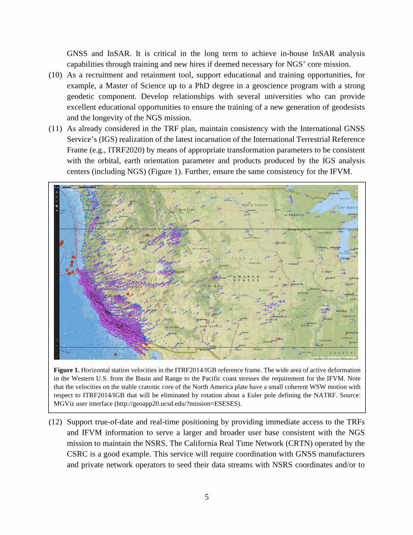
(11) As already considered in the TRF plan, maintain consistency with the International GNSS Service’s (IGS) realization of the latest incarnation of the International Terrestrial Reference Frame (e.g., ITRF2020) by means of appropriate transformation parameters to be consistent with the orbital, earth orientation parameter and products produced by the IGS analysis centers (including NGS) (Figure 1). Further, ensure the same consistency for the IFVM.

(12) Support true-of-date and real-time positioning by providing immediate access to the TRFs and IFVM information to serve a larger and broader user base consistent with the NGS mission to maintain the NSRS. The California Real Time Network (CRTN) operated by the CSRC is a good example. This service will require coordination with GNSS manufacturers and private network operators to seed their data streams with NSRS coordinates and/or to

Figure 1. Horizontal station velocities in the ITRF2014/IGB reference frame. The wide area of active deformation in the Western U.S. from the Basin and Range to the Pacific coast stresses the requirement for the IFVM. Note that the velocities on the stable cratonic core of the North America plate have a small coherent WSW motion with respect to ITRF2014/IGB that will be eliminated by rotation about a Euler pole defining the NATRF. Source: MGViz user interface (http://geoapp20.ucsd.edu/?mission=ESESES).

6

include the proper transformation to the new TRFs in their data controllers. This support is critical for the continued relevance of the NSRS and NGS.

(13) Reconsider consolidating the four reference frames into a single frame tied to the IGS at the designated NSRS reference epoch through the definition of a single Euler pole for the stable North America craton. Since the three frames other than NATRF2020 are intended for networks in deforming regions (Caribbean, Pacific islands, Marianas and north Marianas chain) and are adjacent to North America, positioning could be facilitated through the IFVM. Another option is to also define a Pacific Euler pole also tied to the IGS frame. Considering that there are limited land masses in the Pacific rim, each island or island chain would only need several stations that could serve as TRF base stations for local positioning needs.

4. Motivation The National Geodetic Survey (NGS) is responsible for maintaining the National Spatial Reference System (NSRS), which will be modernized with the introduction of four new geometric reference frames as the source of geodetic latitude, longitude and height:

• North American Terrestrial Reference Frame of 2022 (NATRF2022) – North America including Northern Mexico

• Pacific Terrestrial Reference Frame of 2022 (PATRF2022) – Hawaii and Samoa • Mariana Terrestrial Reference Frame of 2022 (MATRF2022) – Guam, Rota, Tinian and

Saipan • Caribbean Terrestrial Reference Frame of 2022 (CATRF2022) – Puerto Rico, and all other

areas in the Caribbean and Central America The new NSRS will also include a vertical geopotential datum, the North American-Pacific Geopotential Datum of 2022 (NAPGD2022), including a time-dependent geoid model, GEOID2022, derived from the GRAV-D observations. Although this scoping study is focused on

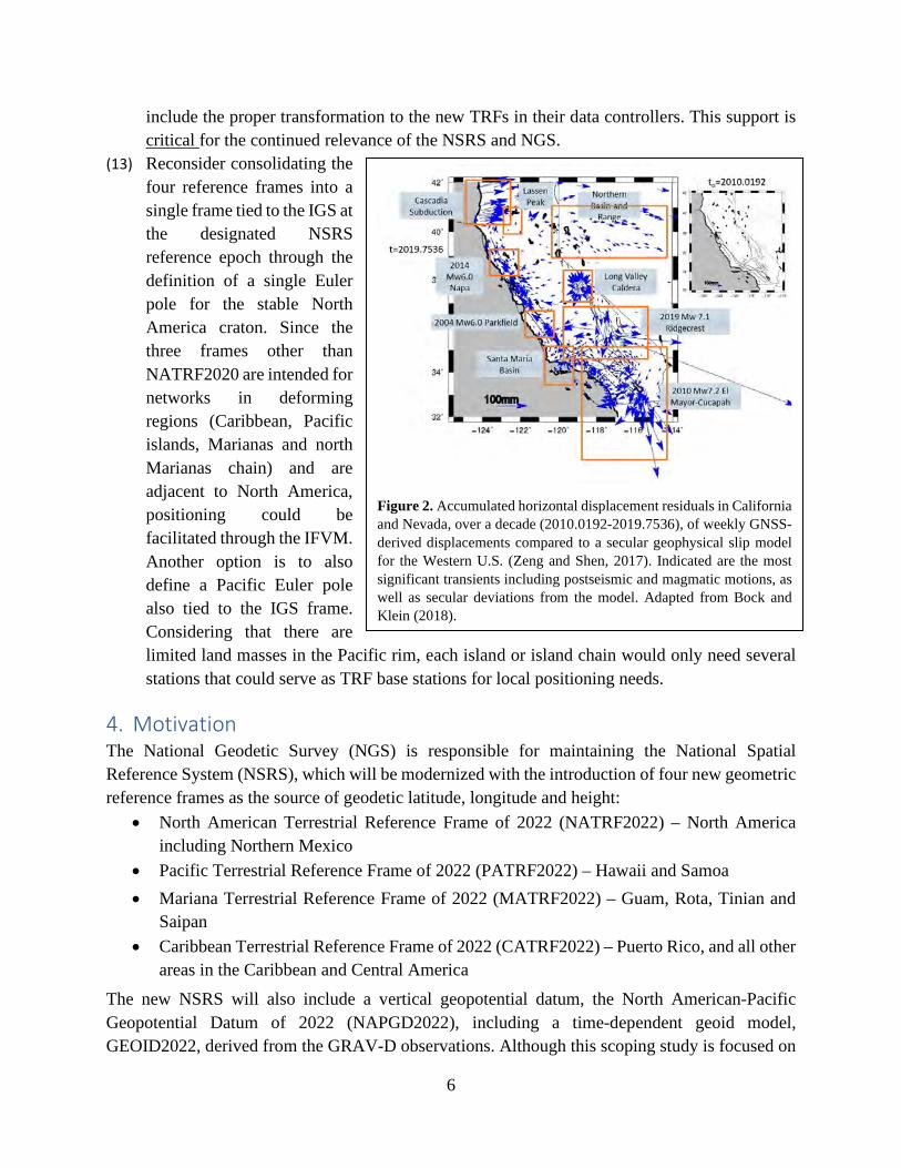
Figure 2. Accumulated horizontal displacement residuals in California and Nevada, over a decade (2010.0192-2019.7536), of weekly GNSS-derived displacements compared to a secular geophysical slip model for the Western U.S. (Zeng and Shen, 2017). Indicated are the most significant transients including postseismic and magmatic motions, as well as secular deviations from the model. Adapted from Bock and Klein (2018).

7

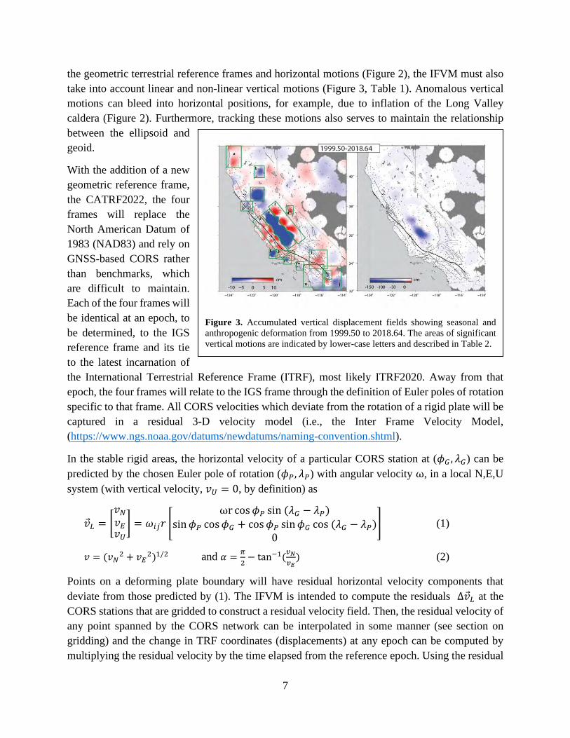
the geometric terrestrial reference frames and horizontal motions (Figure 2), the IFVM must also take into account linear and non-linear vertical motions (Figure 3, Table 1). Anomalous vertical motions can bleed into horizontal positions, for example, due to inflation of the Long Valley caldera (Figure 2). Furthermore, tracking these motions also serves to maintain the relationship between the ellipsoid and geoid.

With the addition of a new geometric reference frame, the CATRF2022, the four frames will replace the North American Datum of 1983 (NAD83) and rely on GNSS-based CORS rather than benchmarks, which are difficult to maintain. Each of the four frames will be identical at an epoch, to be determined, to the IGS reference frame and its tie to the latest incarnation of the International Terrestrial Reference Frame (ITRF), most likely ITRF2020. Away from that epoch, the four frames will relate to the IGS frame through the definition of Euler poles of rotation specific to that frame. All CORS velocities which deviate from the rotation of a rigid plate will be captured in a residual 3-D velocity model (i.e., the Inter Frame Velocity Model, (https://www.ngs.noaa.gov/datums/newdatums/naming-convention.shtml).

In the stable rigid areas, the horizontal velocity of a particular CORS station at (𝜙𝜙𝐺𝐺 , 𝜆𝜆𝐺𝐺) can be predicted by the chosen Euler pole of rotation (𝜙𝜙𝑃𝑃, 𝜆𝜆𝑃𝑃) with angular velocity ω, in a local N,E,U system (with vertical velocity, 𝑣𝑣𝑈𝑈 = 0, by definition) as

�⃗�𝑣𝐿𝐿 = �𝑣𝑣𝑁𝑁𝑣𝑣𝐸𝐸𝑣𝑣𝑈𝑈� = 𝜔𝜔𝑖𝑖𝑖𝑖𝑟𝑟 �

ωr cos𝜙𝜙𝑃𝑃 sin (𝜆𝜆𝐺𝐺 − 𝜆𝜆𝑃𝑃)sin𝜙𝜙𝑃𝑃 cos𝜙𝜙𝐺𝐺 + cos𝜙𝜙𝑃𝑃 sin𝜙𝜙𝐺𝐺 cos (𝜆𝜆𝐺𝐺 − 𝜆𝜆𝑃𝑃)

0� (1)

𝑣𝑣 = (𝑣𝑣𝑁𝑁2 + 𝑣𝑣𝐸𝐸2)1/2 and 𝛼𝛼 = 𝜋𝜋2− tan−1(𝑣𝑣𝑁𝑁

𝑣𝑣𝐸𝐸) (2)

Points on a deforming plate boundary will have residual horizontal velocity components that deviate from those predicted by (1). The IFVM is intended to compute the residuals Δ�⃗�𝑣𝐿𝐿 at the CORS stations that are gridded to construct a residual velocity field. Then, the residual velocity of any point spanned by the CORS network can be interpolated in some manner (see section on gridding) and the change in TRF coordinates (displacements) at any epoch can be computed by multiplying the residual velocity by the time elapsed from the reference epoch. Using the residual

Figure 3. Accumulated vertical displacement fields showing seasonal and anthropogenic deformation from 1999.50 to 2018.64. The areas of significant vertical motions are indicated by lower-case letters and described in Table 2.

8

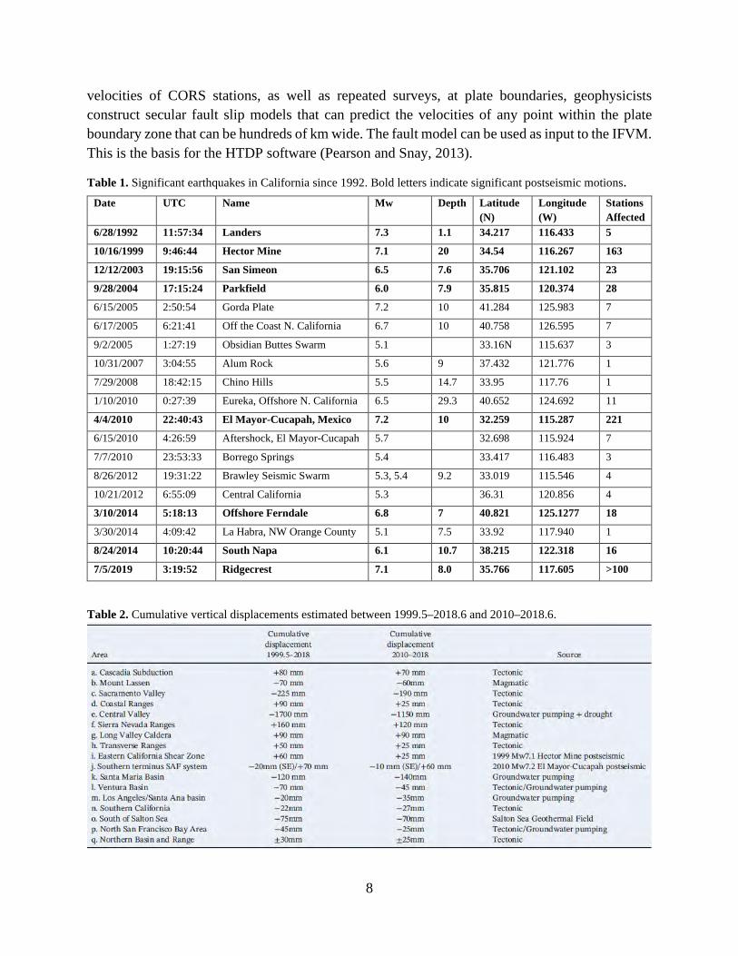
velocities of CORS stations, as well as repeated surveys, at plate boundaries, geophysicists construct secular fault slip models that can predict the velocities of any point within the plate boundary zone that can be hundreds of km wide. The fault model can be used as input to the IFVM. This is the basis for the HTDP software (Pearson and Snay, 2013).

Table 1. Significant earthquakes in California since 1992. Bold letters indicate significant postseismic motions. Date UTC Name Mw Depth Latitude

(N) Longitude (W)

Stations Affected

6/28/1992 11:57:34 Landers 7.3 1.1 34.217 116.433 5

10/16/1999 9:46:44 Hector Mine 7.1 20 34.54 116.267 163

12/12/2003 19:15:56 San Simeon 6.5 7.6 35.706 121.102 23

9/28/2004 17:15:24 Parkfield 6.0 7.9 35.815 120.374 28

6/15/2005 2:50:54 Gorda Plate 7.2 10 41.284 125.983 7

6/17/2005 6:21:41 Off the Coast N. California 6.7 10 40.758 126.595 7

9/2/2005 1:27:19 Obsidian Buttes Swarm 5.1 33.16N 115.637 3

10/31/2007 3:04:55 Alum Rock 5.6 9 37.432 121.776 1

7/29/2008 18:42:15 Chino Hills 5.5 14.7 33.95 117.76 1

1/10/2010 0:27:39 Eureka, Offshore N. California 6.5 29.3 40.652 124.692 11

4/4/2010 22:40:43 El Mayor-Cucapah, Mexico 7.2 10 32.259 115.287 221

6/15/2010 4:26:59 Aftershock, El Mayor-Cucapah 5.7

32.698 115.924 7

7/7/2010 23:53:33 Borrego Springs 5.4

33.417 116.483 3

8/26/2012 19:31:22 Brawley Seismic Swarm 5.3, 5.4 9.2 33.019 115.546 4

10/21/2012 6:55:09 Central California 5.3

36.31 120.856 4

3/10/2014 5:18:13 Offshore Ferndale 6.8 7 40.821 125.1277 18

3/30/2014 4:09:42 La Habra, NW Orange County 5.1 7.5 33.92 117.940 1

8/24/2014 10:20:44 South Napa 6.1 10.7 38.215 122.318 16

7/5/2019 3:19:52 Ridgecrest 7.1 8.0 35.766 117.605 >100

Table 2. Cumulative vertical displacements estimated between 1999.5–2018.6 and 2010–2018.6.

9

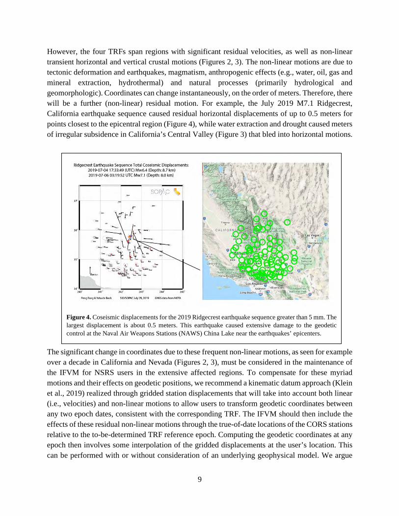
However, the four TRFs span regions with significant residual velocities, as well as non-linear transient horizontal and vertical crustal motions (Figures 2, 3). The non-linear motions are due to tectonic deformation and earthquakes, magmatism, anthropogenic effects (e.g., water, oil, gas and mineral extraction, hydrothermal) and natural processes (primarily hydrological and geomorphologic). Coordinates can change instantaneously, on the order of meters. Therefore, there will be a further (non-linear) residual motion. For example, the July 2019 M7.1 Ridgecrest, California earthquake sequence caused residual horizontal displacements of up to 0.5 meters for points closest to the epicentral region (Figure 4), while water extraction and drought caused meters of irregular subsidence in California’s Central Valley (Figure 3) that bled into horizontal motions.

The significant change in coordinates due to these frequent non-linear motions, as seen for example over a decade in California and Nevada (Figures 2, 3), must be considered in the maintenance of the IFVM for NSRS users in the extensive affected regions. To compensate for these myriad motions and their effects on geodetic positions, we recommend a kinematic datum approach (Klein et al., 2019) realized through gridded station displacements that will take into account both linear (i.e., velocities) and non-linear motions to allow users to transform geodetic coordinates between any two epoch dates, consistent with the corresponding TRF. The IFVM should then include the effects of these residual non-linear motions through the true-of-date locations of the CORS stations relative to the to-be-determined TRF reference epoch. Computing the geodetic coordinates at any epoch then involves some interpolation of the gridded displacements at the user’s location. This can be performed with or without consideration of an underlying geophysical model. We argue

Figure 4. Coseismic displacements for the 2019 Ridgecrest earthquake sequence greater than 5 mm. The largest displacement is about 0.5 meters. This earthquake caused extensive damage to the geodetic control at the Naval Air Weapons Stations (NAWS) China Lake near the earthquakes’ epicenters.

10

that a geophysical model is required for a GNSS CORS network in order to account for elastic surface motions near faults. The introduction of InSAR displacements, where feasible, may replace the need for an underlying geophysical model. Of course, equation (1) predicts no expected vertical motions. Nevertheless, as indicated earlier, linear and non-linear vertical motions need to be considered since they bleed into horizontal motions. Since it is difficult to model vertical motions, we recommend to simply interpolate the vertical motions at the CORS stations (Figure 3) as described in Klein et al. (2019).

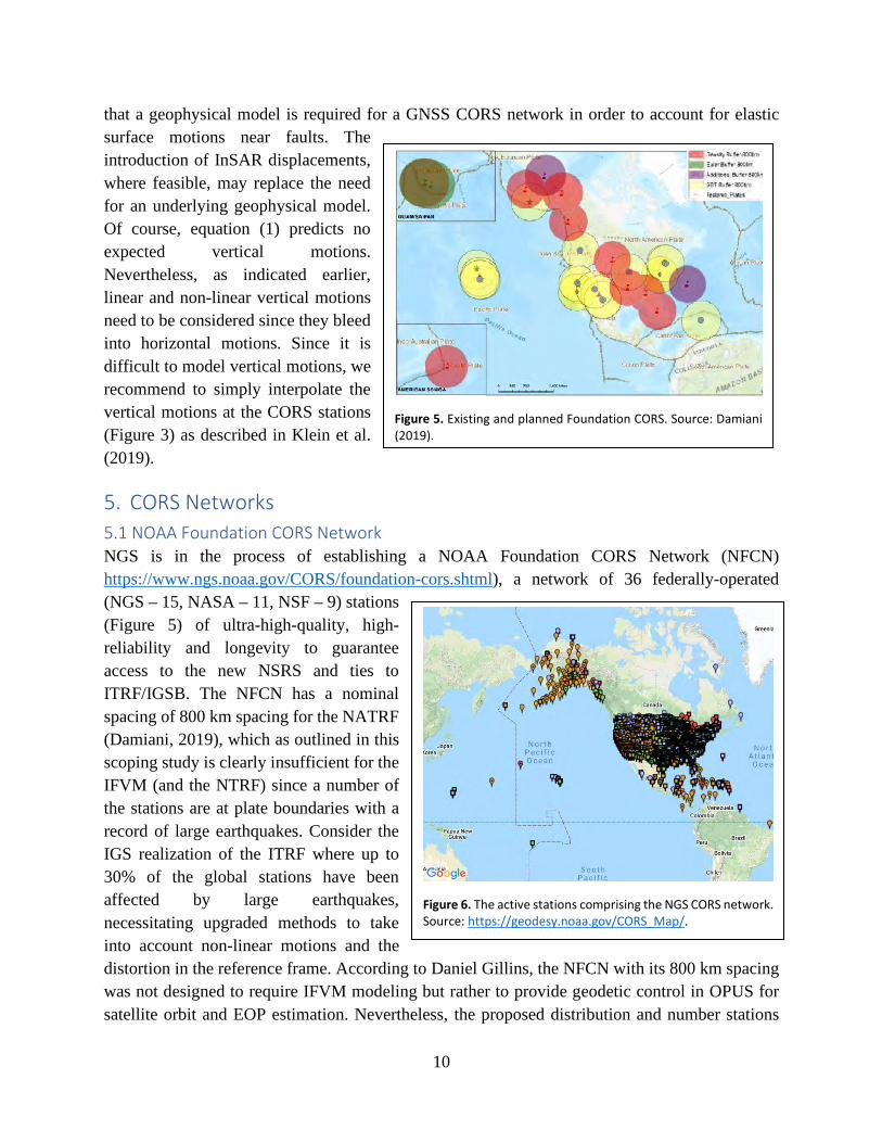
5. CORS Networks 5.1 NOAA Foundation CORS Network NGS is in the process of establishing a NOAA Foundation CORS Network (NFCN) https://www.ngs.noaa.gov/CORS/foundation-cors.shtml), a network of 36 federally-operated (NGS – 15, NASA – 11, NSF – 9) stations (Figure 5) of ultra-high-quality, high-reliability and longevity to guarantee access to the new NSRS and ties to ITRF/IGSB. The NFCN has a nominal spacing of 800 km spacing for the NATRF (Damiani, 2019), which as outlined in this scoping study is clearly insufficient for the IFVM (and the NTRF) since a number of the stations are at plate boundaries with a record of large earthquakes. Consider the IGS realization of the ITRF where up to 30% of the global stations have been affected by large earthquakes, necessitating upgraded methods to take into account non-linear motions and the distortion in the reference frame. According to Daniel Gillins, the NFCN with its 800 km spacing was not designed to require IFVM modeling but rather to provide geodetic control in OPUS for satellite orbit and EOP estimation. Nevertheless, the proposed distribution and number stations

Figure 5. Existing and planned Foundation CORS. Source: Damiani (2019).

Figure 6. The active stations comprising the NGS CORS network. Source: https://geodesy.noaa.gov/CORS_Map/.

11

will affect these products through non-linear motions of many of the stations and needs to be considered.

5.2 Other CORS stations Other than the NFCN, the remaining CORS stations (Figure 6) are maintained by other groups and made available to NGS through cooperative agreements. There are at least 3 CORS stations over CONUS and most parts of Alaska within a nominal 250 km radius. CORS station spacing in the areas of active deformation is much tighter but still does not take advantage of the majority of available cGNSS stations required for interpolation of coordinate corrections within fault regions with linear and non-linear motions.

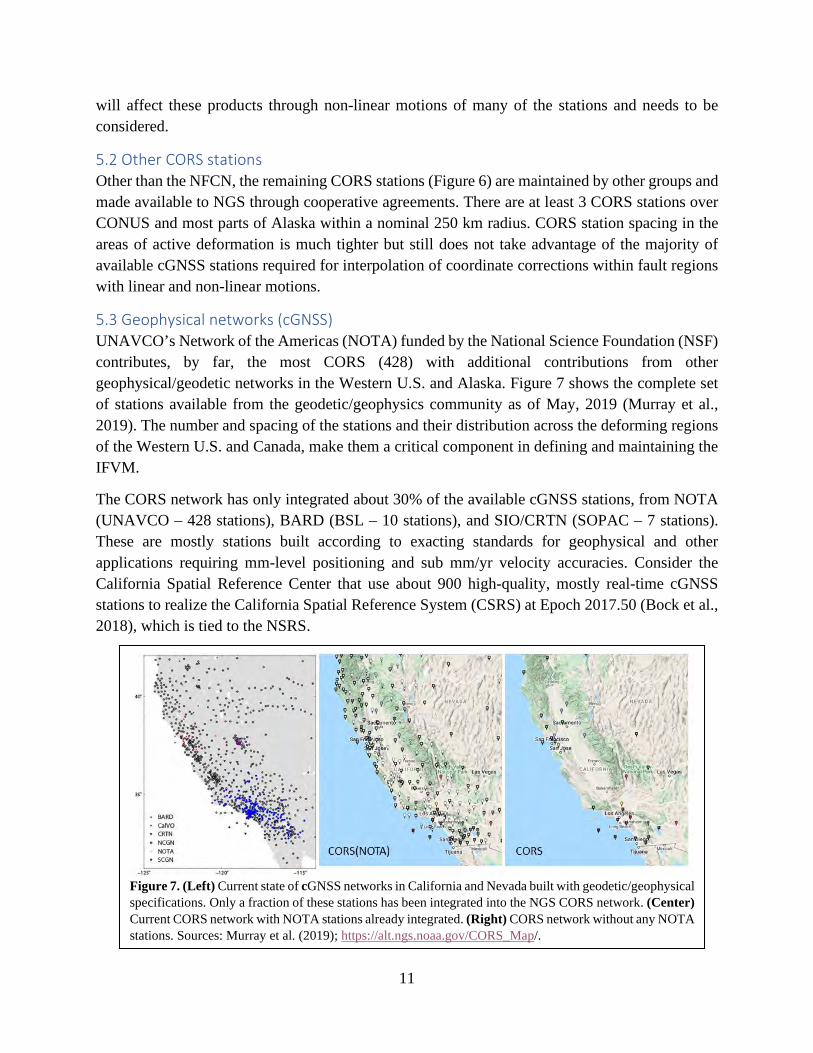
5.3 Geophysical networks (cGNSS) UNAVCO’s Network of the Americas (NOTA) funded by the National Science Foundation (NSF) contributes, by far, the most CORS (428) with additional contributions from other geophysical/geodetic networks in the Western U.S. and Alaska. Figure 7 shows the complete set of stations available from the geodetic/geophysics community as of May, 2019 (Murray et al., 2019). The number and spacing of the stations and their distribution across the deforming regions of the Western U.S. and Canada, make them a critical component in defining and maintaining the IFVM.

The CORS network has only integrated about 30% of the available cGNSS stations, from NOTA (UNAVCO – 428 stations), BARD (BSL – 10 stations), and SIO/CRTN (SOPAC – 7 stations). These are mostly stations built according to exacting standards for geophysical and other applications requiring mm-level positioning and sub mm/yr velocity accuracies. Consider the California Spatial Reference Center that use about 900 high-quality, mostly real-time cGNSS stations to realize the California Spatial Reference System (CSRS) at Epoch 2017.50 (Bock et al., 2018), which is tied to the NSRS.

Figure 7. (Left) Current state of cGNSS networks in California and Nevada built with geodetic/geophysical specifications. Only a fraction of these stations has been integrated into the NGS CORS network. (Center) Current CORS network with NOTA stations already integrated. (Right) CORS network without any NOTA stations. Sources: Murray et al. (2019); https://alt.ngs.noaa.gov/CORS_Map/.

12

5.4 Longevity The most critical issues for the TRFs is the long-term availability of CORS stations. There are currently 131 diverse data sources that operate anywhere from 1 to 428 stations (https://geodesy.noaa.gov/CORS/). The bulk of the stations are operated by departments of transportations and geodetic surveys. There are 20 departments of transportation networks that have been integrated into the CORS network – the largest contributor is the Texas Department of Transportation with 148 stations. The dependence on state-wide agencies, ensures longevity, as long as the long-term relationships are maintained.

The geophysical/geodetic networks are primarily funded by NSF, NASA and other federal agencies as science projects are subject to periodic (~5 year) review. Therefore, their longevity is not guaranteed. However, many of the stations are being integrated into California’s earthquake early warning system, for example, and there is an ongoing effort to transition some NOTA stations to state agencies such as Caltrans. Conspicuously missing from the current CORS network are the USGS stations (SCGN – Figure 7) and Caltrans-owned stations of the Central Valley Spatial

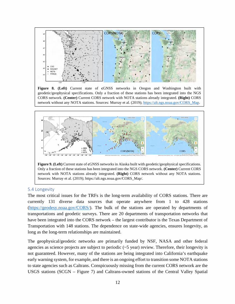
Figure 9. (Left) Current state of cGNSS networks in Alaska built with geodetic/geophysical specifications. Only a fraction of these stations has been integrated into the NGS CORS network. (Center) Current CORS network with NOTA stations already integrated. (Right) CORS network without any NOTA stations. Sources: Murray et al. (2019); https://alt.ngs.noaa.gov/CORS_Map/.

Figure 8. (Left) Current state of cGNSS networks in Oregon and Washington built with geodetic/geophysical specifications. Only a fraction of these stations has been integrated into the NGS CORS network. (Center) Current CORS network with NOTA stations already integrated. (Right) CORS network without any NOTA stations. Sources: Murray et al. (2019); https://alt.ngs.noaa.gov/CORS_Map.

13

Reference Network (CVSRN) and Central Coast Reference Network (CCSRN), which are expected to operate for the long term. In the Pacific Northwest (Figure 7), there are two main networks, NOTA (~30 CORS) and PANGA (~25 CORS). PANGA includes stations from the Washington Spatial Reference Network and the Oregon Department of Transportation. The Alaska stations are nearly all part of NOTA.

It is critical that NGS becomes involved with federal agencies (NASA, NSF, USGS) to advocate for the continuation of the cGNSS networks in terms of joint funding, partnerships and community adoptions to support the NSRS and IFVM into the long term and for the overall public good.

5.5 CORS Analysis The maintenance of the IFVM requires regular analysis of the CORS data, in particular in the areas of significant crustal motions that may be subject to transient events, e.g., coseismic and postseismic motions (Figures 2,3). In order to respond quickly to significant non-linear changes in coordinates, a robust underlying analysis infrastructure and user interface should be established and maintained. We understand that the full complement of CORS GNSS data are not analyzed on a regular basis, unlike other U.S.-based groups that perform daily solutions of stations within the zones of crustal motion (e.g., Nevada Geodetic Laboratory, Scripps Orbit and Permanent Array Center, Jet Propulsion Laboratory, U.S. Geological Survey, Central Washington University). We recommend that NGS perform regular analysis of the CORS stations. The NGS group already produces IGS products as one of its analysis centers and is well versed in GNSS data analysis. It may be necessary to add 1-2 additional staff member to this group. At least a weekly cadence is recommended and daily when a significant event occurs (e.g., large earthquake). One alternative is to sub-contract the daily analysis to an outside group. However, since these are primarily university or research groups, analysis expertise should be maintained in house at NGS for the long term.

5.6 Reliability & quality control Regular analysis of the CORS data provide an important quality control role, an essential component for long-term maintenance of the TRFs and IFVM. The CORS stations should be regularly evaluated and graded in order to identify and exclude any poorly performing stations. This includes: (1) Accurate and timely metadata, in particular changes in antenna model and height, in a modern

database. Late and/or inaccurate metadata will introduce spurious offsets into the displacement time series, as well as loss of precision, necessitating re-analysis. Stations photos are a useful resource for quality control.

(2) Completeness and timeliness of station Data that do not arrive on time cause gaps in the time series. However, missing data can be back-filled prior to a re-analysis of earlier data holdings.

(3) Gross errors in the a priori coordinates can adversely affect data analysis and result in gaps in the displacement time series. These can be due to geophysical signals (e.g., large coseismic displacements), inaccurate metadata or problems in the GPS analysis.

14

(4) Large adjustments from the a priori coordinates should be flagged and reviewed as quickly as possible.

(5) Examination of displacement time series: 1. Catalogue offsets due to

coseismic deformation, and other jumps due to unlike antenna changes, for example.

2. Identify and categorize any deviations from linearity, outliers

3. Identify stations with anomalous local motions (e.g., landslides)

4. Document gaps in the data to identify problematic stations

5. Identify and exclude outliers – study machine learning methods.

6. Assign simple QC ratings (e.g., Excellent, Very Good, Good, Fair, Poor)

(6) Regular station by station monitoring of raw GPS data for anomalous behavior, for example, multipath, cycle slips, signal to noise ratio, ionospheric effects and seasonal variations (e.g., Estey and Meertens, 1999; Hilla, 2002; Ogaja and Hedfors, 2007; Lee et al., 2012).

(7) Often, interactive examination of the displacement time series is required to identify and flag problematic time series so this capability should be available.

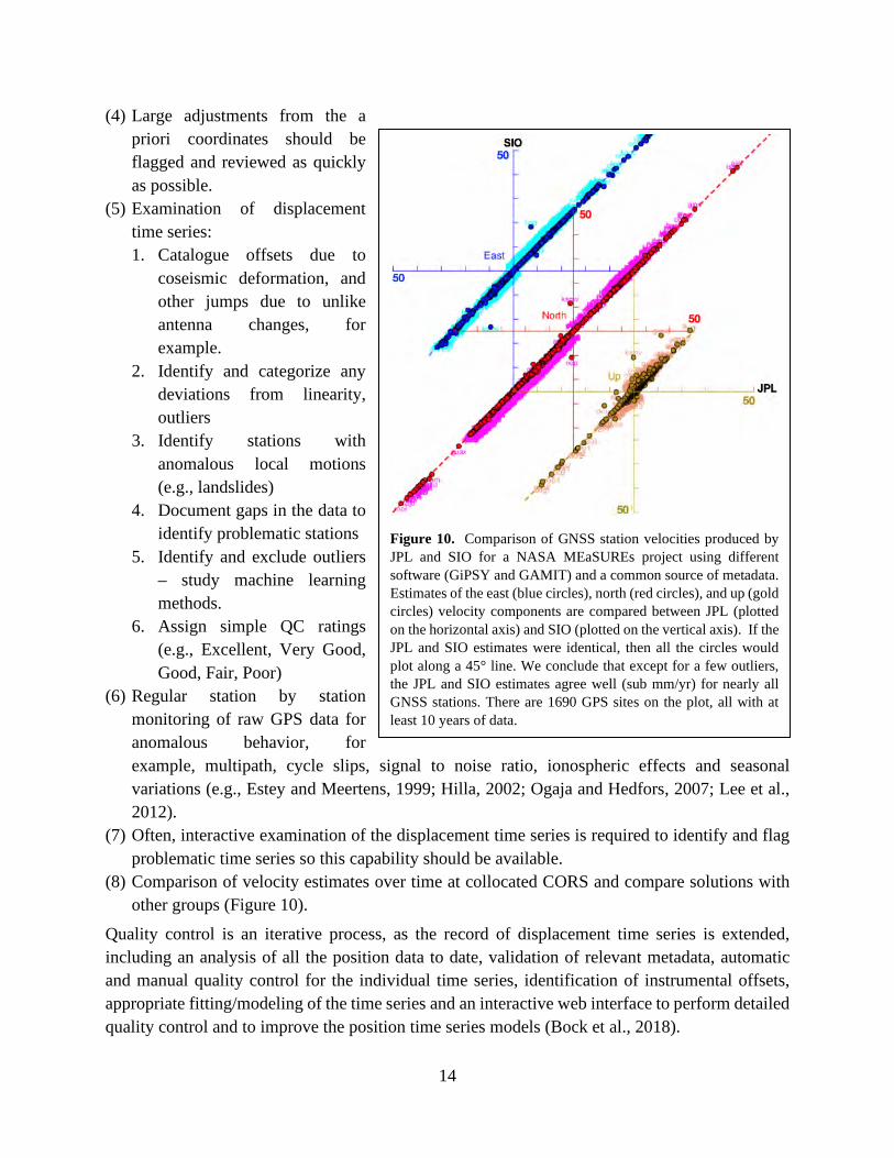
(8) Comparison of velocity estimates over time at collocated CORS and compare solutions with other groups (Figure 10).

Quality control is an iterative process, as the record of displacement time series is extended, including an analysis of all the position data to date, validation of relevant metadata, automatic and manual quality control for the individual time series, identification of instrumental offsets, appropriate fitting/modeling of the time series and an interactive web interface to perform detailed quality control and to improve the position time series models (Bock et al., 2018).

Figure 10. Comparison of GNSS station velocities produced by JPL and SIO for a NASA MEaSUREs project using different software (GiPSY and GAMIT) and a common source of metadata. Estimates of the east (blue circles), north (red circles), and up (gold circles) velocity components are compared between JPL (plotted on the horizontal axis) and SIO (plotted on the vertical axis). If the JPL and SIO estimates were identical, then all the circles would plot along a 45° line. We conclude that except for a few outliers, the JPL and SIO estimates agree well (sub mm/yr) for nearly all GNSS stations. There are 1690 GPS sites on the plot, all with at least 10 years of data.

15

6. Proposed IFVM Methodology Here we expand on the motivation for an IFVM and the issue of significant non-linear motions and propose an IVFM methodology based on a kinematic reference frame approach described by Klein et al. (2019) using residual GNSS and (where available) InSAR displacement grids.

A user requires knowledge of the motions of an arbitrary station to seamlessly transform coordinates between any two dates with respect to a TRF by implementing an IFVM to compute residual velocities Δ�⃗�𝑣𝐿𝐿 (equation 1) for non-rigid locations spanned by the TRF. Two sources of information are available. The first source is a grid of surface velocities (velocity field) estimated from daily displacement time series. The grid represents the physical (secular, time independent) residual motions of the stations with respect to a TRF at a particular epoch of time. The displacement grid can then be interpolated at any location within the network; the expected displacements are just the velocity components multiplied by the time interval from the reference epoch (e.g., 2022.00). However, there are a myriad of interpolation methods to choose from, which are discussed later.

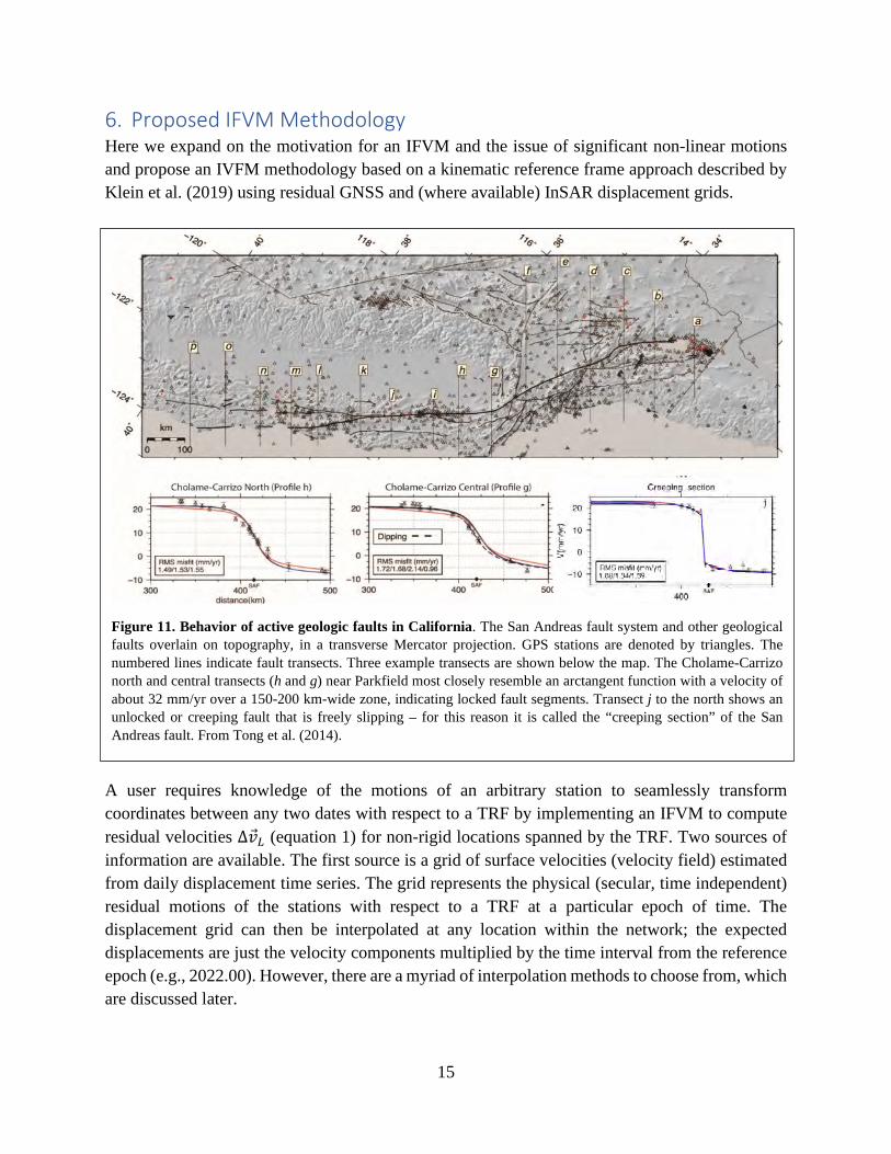
Figure 11. Behavior of active geologic faults in California. The San Andreas fault system and other geological faults overlain on topography, in a transverse Mercator projection. GPS stations are denoted by triangles. The numbered lines indicate fault transects. Three example transects are shown below the map. The Cholame-Carrizo north and central transects (h and g) near Parkfield most closely resemble an arctangent function with a velocity of about 32 mm/yr over a 150-200 km-wide zone, indicating locked fault segments. Transect j to the north shows an unlocked or creeping fault that is freely slipping – for this reason it is called the “creeping section” of the San Andreas fault. From Tong et al. (2014).

16

The second source of information is an underlying secular fault slip model that predicts the surface displacements at any location and time. This is the basis of the Horizontal Time-Dependent Positioning (HTDP) software (Pearson and Snay, 2013; https://geodesy.noaa.gov/TOOLS/Htdp/Htdp.shtml). It is important to understand why a geophysical model is useful. Fault slip at depth manifests itself as surface displacements when viewed as orthogonal to the fault trace, resemble, according to elastic rebound theory (e.g., Savage and Burford, 1973), an inverse tangent function for a locked fault (see transects g and h) or as a step function (transect j) for a creeping fault that is freely slipping (Figure 11). Simply stated, the predicted surface motions decrease with distance away from a fault as a function of its depth and the degree of locking on the fault interface (locked vs. creep). Models have been developed for secular interseismic motions, coseismic deformation and transient postseismic decay that can be used to predict surface motions. Note that the locations of cGNSS and survey markers for crustal deformation research are chosen to best represent the expected motions and elucidate fault slip at depth and not according to some arbitrary grid spacing.

Many horizontal crustal deformation models have been published for different parts of the Western U.S. (Bock and Melgar, 2016, and references therein) and for the entire region (Zeng and Shen 2017). As new observations and new physical insights become available, geophysical models evolve. However, they are inherently ill-determined and non-unique and require statistical methods, physical constraints and intuition to be determinable.

The maintenance of an IFVM (and TRF, for that matter) solely from velocity vectors is complicated by episodic (coseismic), longer-term (postseismic) and other time variable transient motions. These motions are difficult to capture through interpolation of surface velocities (or displacements) alone. In practice in the development of interseismic models, non-secular motions are taken into account by (subjectively) disregarding parts of the (daily) displacement time series or by modeling the transient motion either parametrically or through a physical postseismic slip model (e.g., Gonzalez et al. 2014). In the event of a large earthquake, such as the July 4-6, 2019 Mw6.4 and Mw7.1 Ridgecrest earthquake sequence, many stations are displaced (Figure 4). Table 1 lists the earthquakes in California since 1992 that caused significant coseismic motions; seven of the earthquakes were following by several years of postseismic motions.

To be most useful to the user community, it is necessary to quickly react to a significant event by publishing corrections to the IFVM. As an example, after the Ridgecrest earthquakes the California Spatial Reference Center (CSRC) estimated within days a new set of coordinates for the affected stations at a new epoch (2019.55) as an update to their Epoch 2017.50 coordinates (Figure 4). (http://sopac-csrc.ucsd.edu/wp-content/uploads/2019/08/PostRidgecrestCoordinatesEpoch_2019.55.txt.

17

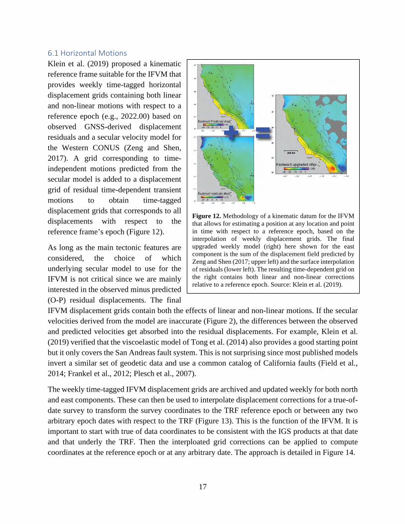
6.1 Horizontal Motions Klein et al. (2019) proposed a kinematic reference frame suitable for the IFVM that provides weekly time-tagged horizontal displacement grids containing both linear and non-linear motions with respect to a reference epoch (e.g., 2022.00) based on observed GNSS-derived displacement residuals and a secular velocity model for the Western CONUS (Zeng and Shen, 2017). A grid corresponding to time-independent motions predicted from the secular model is added to a displacement grid of residual time-dependent transient motions to obtain time-tagged displacement grids that corresponds to all displacements with respect to the reference frame’s epoch (Figure 12).

As long as the main tectonic features are considered, the choice of which underlying secular model to use for the IFVM is not critical since we are mainly interested in the observed minus predicted (O-P) residual displacements. The final IFVM displacement grids contain both the effects of linear and non-linear motions. If the secular velocities derived from the model are inaccurate (Figure 2), the differences between the observed and predicted velocities get absorbed into the residual displacements. For example, Klein et al. (2019) verified that the viscoelastic model of Tong et al. (2014) also provides a good starting point but it only covers the San Andreas fault system. This is not surprising since most published models invert a similar set of geodetic data and use a common catalog of California faults (Field et al., 2014; Frankel et al., 2012; Plesch et al., 2007).

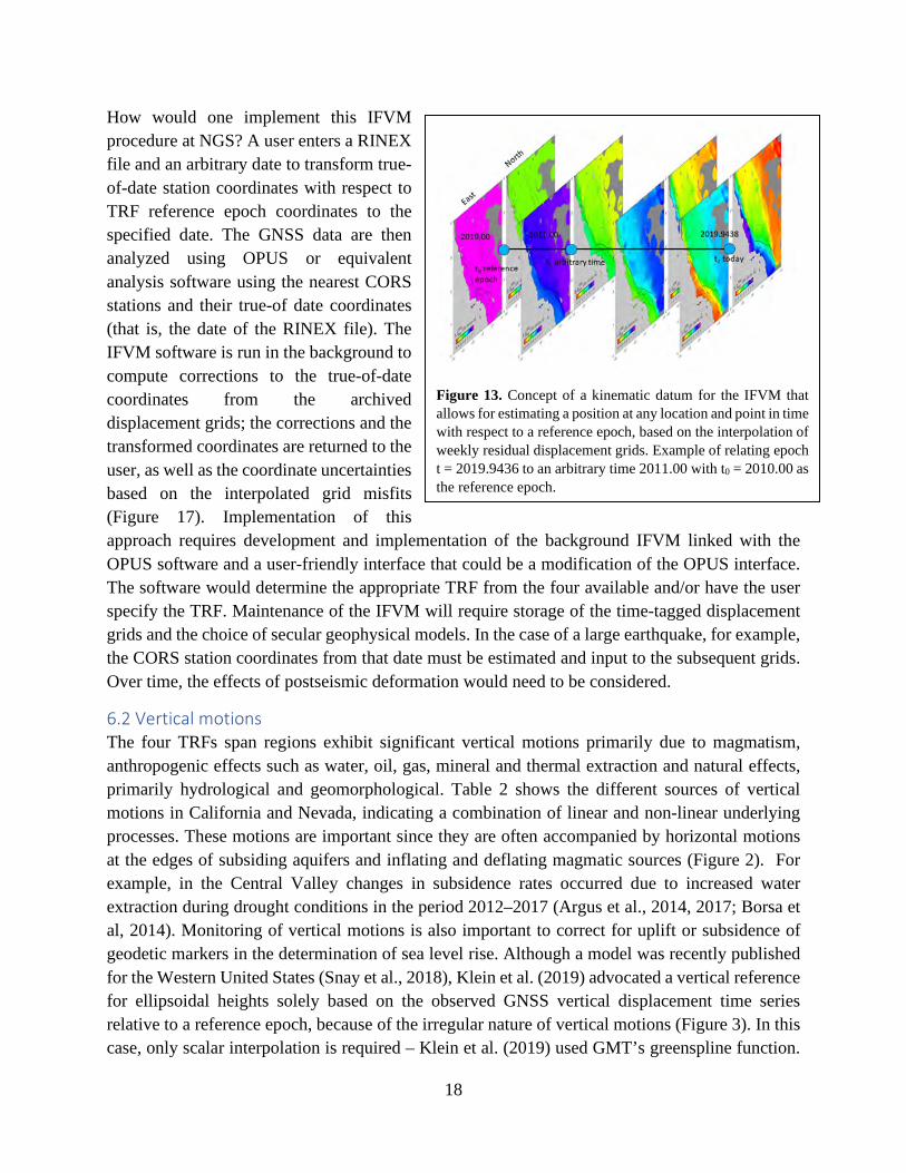
The weekly time-tagged IFVM displacement grids are archived and updated weekly for both north and east components. These can then be used to interpolate displacement corrections for a true-of-date survey to transform the survey coordinates to the TRF reference epoch or between any two arbitrary epoch dates with respect to the TRF (Figure 13). This is the function of the IFVM. It is important to start with true of data coordinates to be consistent with the IGS products at that date and that underly the TRF. Then the interploated grid corrections can be applied to compute coordinates at the reference epoch or at any arbitrary date. The approach is detailed in Figure 14.

Figure 12. Methodology of a kinematic datum for the IFVM that allows for estimating a position at any location and point in time with respect to a reference epoch, based on the interpolation of weekly displacement grids. The final upgraded weekly model (right) here shown for the east component is the sum of the displacement field predicted by Zeng and Shen (2017; upper left) and the surface interpolation of residuals (lower left). The resulting time-dependent grid on the right contains both linear and non-linear corrections relative to a reference epoch. Source: Klein et al. (2019).

18

How would one implement this IFVM procedure at NGS? A user enters a RINEX file and an arbitrary date to transform true-of-date station coordinates with respect to TRF reference epoch coordinates to the specified date. The GNSS data are then analyzed using OPUS or equivalent analysis software using the nearest CORS stations and their true-of date coordinates (that is, the date of the RINEX file). The IFVM software is run in the background to compute corrections to the true-of-date coordinates from the archived displacement grids; the corrections and the transformed coordinates are returned to the user, as well as the coordinate uncertainties based on the interpolated grid misfits (Figure 17). Implementation of this approach requires development and implementation of the background IFVM linked with the OPUS software and a user-friendly interface that could be a modification of the OPUS interface. The software would determine the appropriate TRF from the four available and/or have the user specify the TRF. Maintenance of the IFVM will require storage of the time-tagged displacement grids and the choice of secular geophysical models. In the case of a large earthquake, for example, the CORS station coordinates from that date must be estimated and input to the subsequent grids. Over time, the effects of postseismic deformation would need to be considered.

6.2 Vertical motions The four TRFs span regions exhibit significant vertical motions primarily due to magmatism, anthropogenic effects such as water, oil, gas, mineral and thermal extraction and natural effects, primarily hydrological and geomorphological. Table 2 shows the different sources of vertical motions in California and Nevada, indicating a combination of linear and non-linear underlying processes. These motions are important since they are often accompanied by horizontal motions at the edges of subsiding aquifers and inflating and deflating magmatic sources (Figure 2). For example, in the Central Valley changes in subsidence rates occurred due to increased water extraction during drought conditions in the period 2012–2017 (Argus et al., 2014, 2017; Borsa et al, 2014). Monitoring of vertical motions is also important to correct for uplift or subsidence of geodetic markers in the determination of sea level rise. Although a model was recently published for the Western United States (Snay et al., 2018), Klein et al. (2019) advocated a vertical reference for ellipsoidal heights solely based on the observed GNSS vertical displacement time series relative to a reference epoch, because of the irregular nature of vertical motions (Figure 3). In this case, only scalar interpolation is required – Klein et al. (2019) used GMT’s greenspline function.

Figure 13. Concept of a kinematic datum for the IFVM that allows for estimating a position at any location and point in time with respect to a reference epoch, based on the interpolation of weekly residual displacement grids. Example of relating epoch t = 2019.9436 to an arbitrary time 2011.00 with t0 = 2010.00 as the reference epoch.

19

In this regard, the addition of InSAR displacements are very useful to identify the extent and magnitude of vertical deformation and locate any non-representative local anomalies.

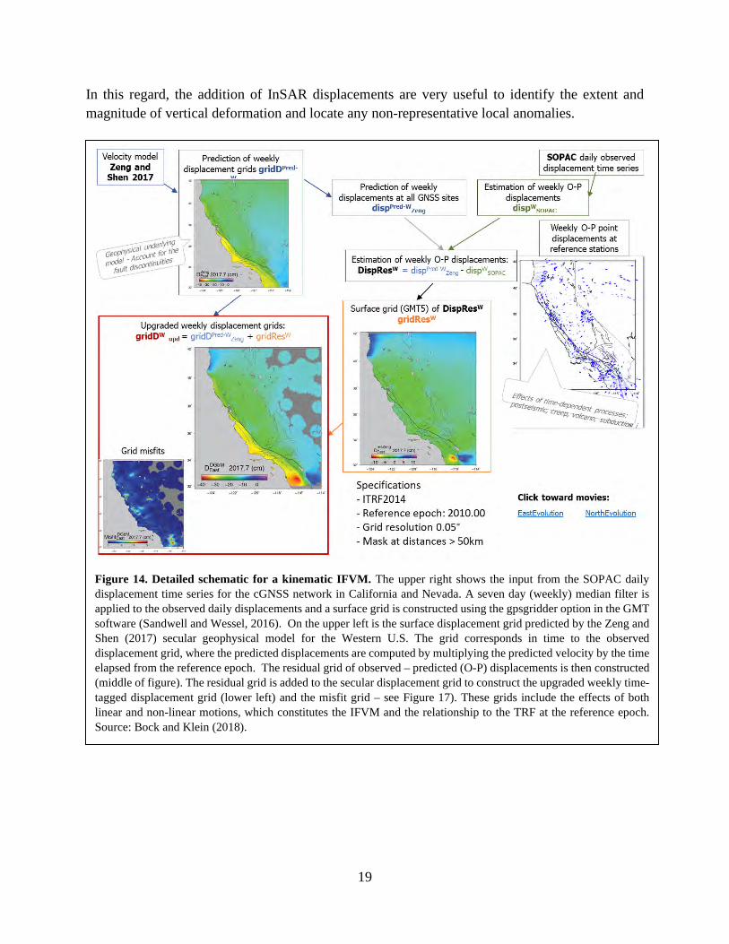
Figure 14. Detailed schematic for a kinematic IFVM. The upper right shows the input from the SOPAC daily displacement time series for the cGNSS network in California and Nevada. A seven day (weekly) median filter is applied to the observed daily displacements and a surface grid is constructed using the gpsgridder option in the GMT software (Sandwell and Wessel, 2016). On the upper left is the surface displacement grid predicted by the Zeng and Shen (2017) secular geophysical model for the Western U.S. The grid corresponds in time to the observed displacement grid, where the predicted displacements are computed by multiplying the predicted velocity by the time elapsed from the reference epoch. The residual grid of observed – predicted (O-P) displacements is then constructed (middle of figure). The residual grid is added to the secular displacement grid to construct the upgraded weekly time-tagged displacement grid (lower left) and the misfit grid – see Figure 17). These grids include the effects of both linear and non-linear motions, which constitutes the IFVM and the relationship to the TRF at the reference epoch. Source: Bock and Klein (2018).

20

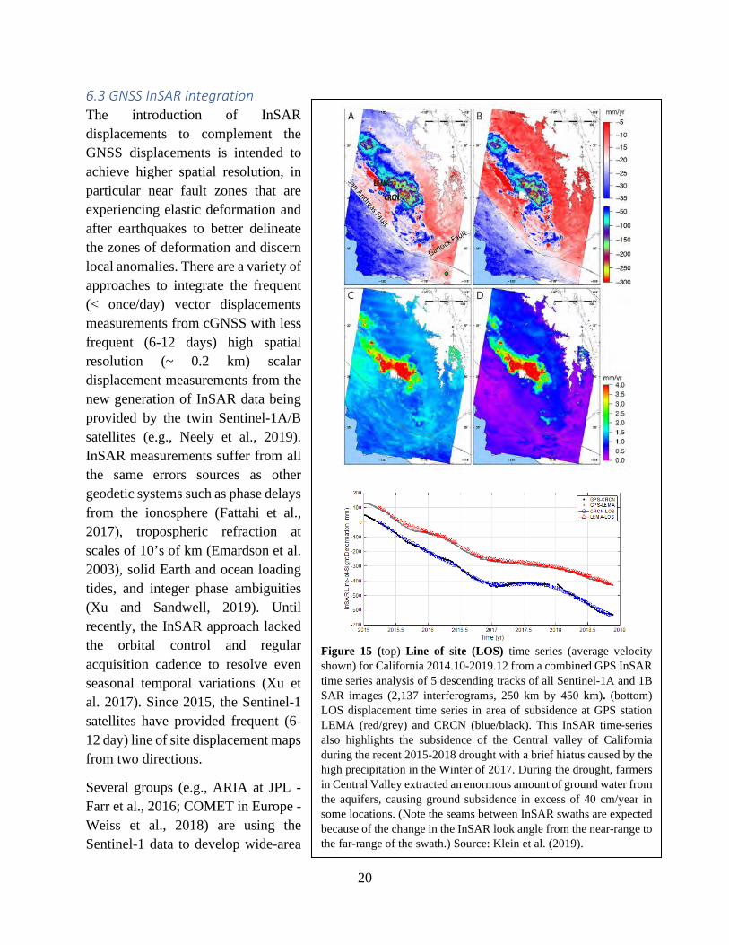
6.3 GNSS InSAR integration The introduction of InSAR displacements to complement the GNSS displacements is intended to achieve higher spatial resolution, in particular near fault zones that are experiencing elastic deformation and after earthquakes to better delineate the zones of deformation and discern local anomalies. There are a variety of approaches to integrate the frequent (< once/day) vector displacements measurements from cGNSS with less frequent (6-12 days) high spatial resolution (~ 0.2 km) scalar displacement measurements from the new generation of InSAR data being provided by the twin Sentinel-1A/B satellites (e.g., Neely et al., 2019). InSAR measurements suffer from all the same errors sources as other geodetic systems such as phase delays from the ionosphere (Fattahi et al., 2017), tropospheric refraction at scales of 10’s of km (Emardson et al. 2003), solid Earth and ocean loading tides, and integer phase ambiguities (Xu and Sandwell, 2019). Until recently, the InSAR approach lacked the orbital control and regular acquisition cadence to resolve even seasonal temporal variations (Xu et al. 2017). Since 2015, the Sentinel-1 satellites have provided frequent (6-12 day) line of site displacement maps from two directions.

Several groups (e.g., ARIA at JPL - Farr et al., 2016; COMET in Europe - Weiss et al., 2018) are using the Sentinel-1 data to develop wide-area

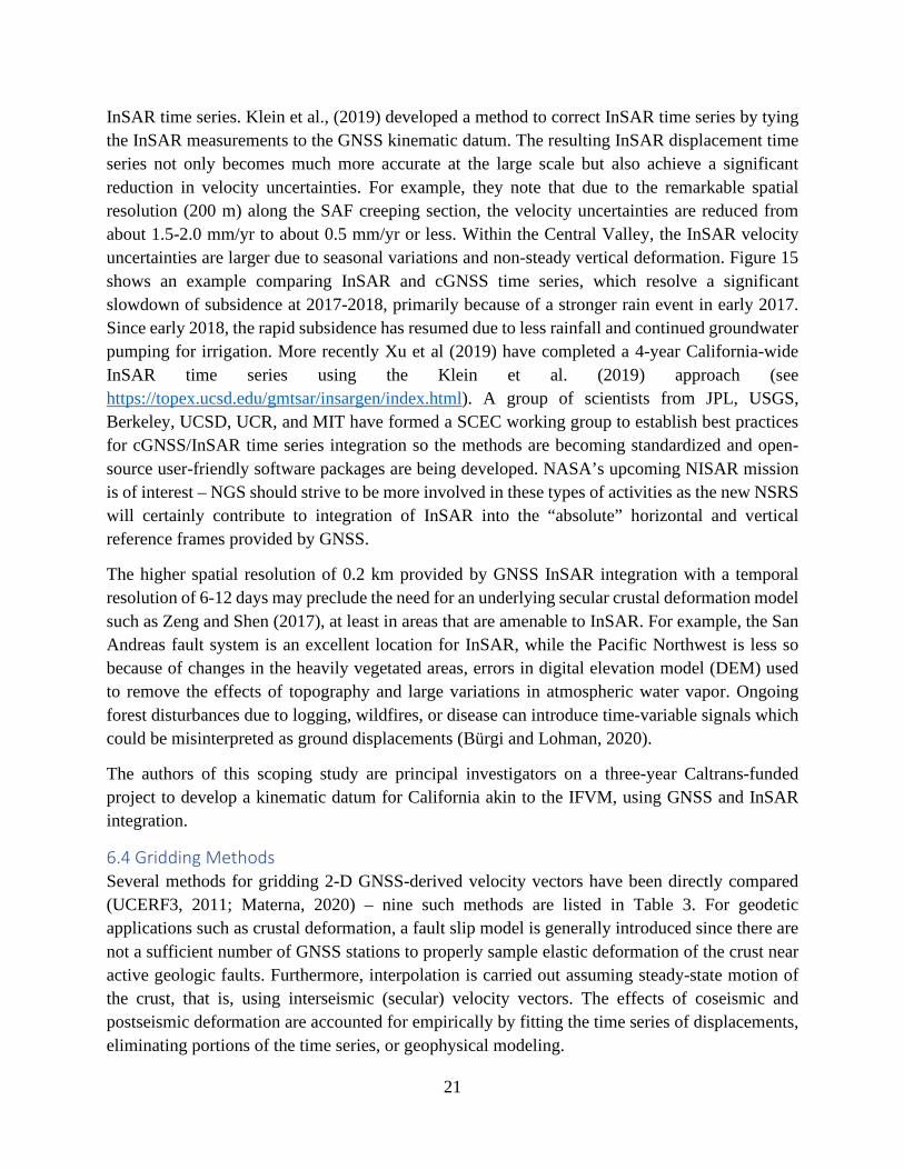
Figure 15 (top) Line of site (LOS) time series (average velocity shown) for California 2014.10-2019.12 from a combined GPS InSAR time series analysis of 5 descending tracks of all Sentinel-1A and 1B SAR images (2,137 interferograms, 250 km by 450 km). (bottom) LOS displacement time series in area of subsidence at GPS station LEMA (red/grey) and CRCN (blue/black). This InSAR time-series also highlights the subsidence of the Central valley of California during the recent 2015-2018 drought with a brief hiatus caused by the high precipitation in the Winter of 2017. During the drought, farmers in Central Valley extracted an enormous amount of ground water from the aquifers, causing ground subsidence in excess of 40 cm/year in some locations. (Note the seams between InSAR swaths are expected because of the change in the InSAR look angle from the near-range to the far-range of the swath.) Source: Klein et al. (2019).

21

InSAR time series. Klein et al., (2019) developed a method to correct InSAR time series by tying the InSAR measurements to the GNSS kinematic datum. The resulting InSAR displacement time series not only becomes much more accurate at the large scale but also achieve a significant reduction in velocity uncertainties. For example, they note that due to the remarkable spatial resolution (200 m) along the SAF creeping section, the velocity uncertainties are reduced from about 1.5-2.0 mm/yr to about 0.5 mm/yr or less. Within the Central Valley, the InSAR velocity uncertainties are larger due to seasonal variations and non-steady vertical deformation. Figure 15 shows an example comparing InSAR and cGNSS time series, which resolve a significant slowdown of subsidence at 2017-2018, primarily because of a stronger rain event in early 2017. Since early 2018, the rapid subsidence has resumed due to less rainfall and continued groundwater pumping for irrigation. More recently Xu et al (2019) have completed a 4-year California-wide InSAR time series using the Klein et al. (2019) approach (see https://topex.ucsd.edu/gmtsar/insargen/index.html). A group of scientists from JPL, USGS, Berkeley, UCSD, UCR, and MIT have formed a SCEC working group to establish best practices for cGNSS/InSAR time series integration so the methods are becoming standardized and open-source user-friendly software packages are being developed. NASA’s upcoming NISAR mission is of interest – NGS should strive to be more involved in these types of activities as the new NSRS will certainly contribute to integration of InSAR into the “absolute” horizontal and vertical reference frames provided by GNSS.

The higher spatial resolution of 0.2 km provided by GNSS InSAR integration with a temporal resolution of 6-12 days may preclude the need for an underlying secular crustal deformation model such as Zeng and Shen (2017), at least in areas that are amenable to InSAR. For example, the San Andreas fault system is an excellent location for InSAR, while the Pacific Northwest is less so because of changes in the heavily vegetated areas, errors in digital elevation model (DEM) used to remove the effects of topography and large variations in atmospheric water vapor. Ongoing forest disturbances due to logging, wildfires, or disease can introduce time-variable signals which could be misinterpreted as ground displacements (Bürgi and Lohman, 2020).

The authors of this scoping study are principal investigators on a three-year Caltrans-funded project to develop a kinematic datum for California akin to the IFVM, using GNSS and InSAR integration.

6.4 Gridding Methods Several methods for gridding 2-D GNSS-derived velocity vectors have been directly compared (UCERF3, 2011; Materna, 2020) – nine such methods are listed in Table 3. For geodetic applications such as crustal deformation, a fault slip model is generally introduced since there are not a sufficient number of GNSS stations to properly sample elastic deformation of the crust near active geologic faults. Furthermore, interpolation is carried out assuming steady-state motion of the crust, that is, using interseismic (secular) velocity vectors. The effects of coseismic and postseismic deformation are accounted for empirically by fitting the time series of displacements, eliminating portions of the time series, or geophysical modeling.

22

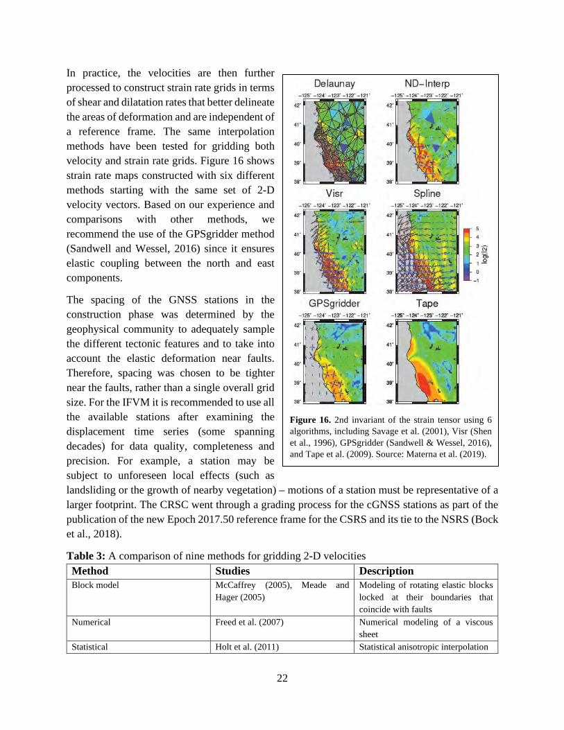
In practice, the velocities are then further processed to construct strain rate grids in terms of shear and dilatation rates that better delineate the areas of deformation and are independent of a reference frame. The same interpolation methods have been tested for gridding both velocity and strain rate grids. Figure 16 shows strain rate maps constructed with six different methods starting with the same set of 2-D velocity vectors. Based on our experience and comparisons with other methods, we recommend the use of the GPSgridder method (Sandwell and Wessel, 2016) since it ensures elastic coupling between the north and east components.

The spacing of the GNSS stations in the construction phase was determined by the geophysical community to adequately sample the different tectonic features and to take into account the elastic deformation near faults. Therefore, spacing was chosen to be tighter near the faults, rather than a single overall grid size. For the IFVM it is recommended to use all the available stations after examining the displacement time series (some spanning decades) for data quality, completeness and precision. For example, a station may be subject to unforeseen local effects (such as landsliding or the growth of nearby vegetation) – motions of a station must be representative of a larger footprint. The CRSC went through a grading process for the cGNSS stations as part of the publication of the new Epoch 2017.50 reference frame for the CSRS and its tie to the NSRS (Bock et al., 2018).

Table 3: A comparison of nine methods for gridding 2-D velocities Method Studies Description Block model McCaffrey (2005), Meade and

Hager (2005) Modeling of rotating elastic blocks locked at their boundaries that coincide with faults

Numerical Freed et al. (2007) Numerical modeling of a viscous sheet

Statistical Holt et al. (2011) Statistical anisotropic interpolation

Figure 16. 2nd invariant of the strain tensor using 6 algorithms, including Savage et al. (2001), Visr (Shen et al., 1996), GPSgridder (Sandwell & Wessel, 2016), and Tape et al. (2009). Source: Materna et al. (2019).

23

2-D interpolation Straightforward interpolation with various weighting schemes (available with Numpy, a Python function)

Delaunay triangulation on a sphere Savage et al. (2001) Similar to 2-D interpolation using a triangular grid (available with Numpy, a Python function)

Visr Shen et al. (1996) Weighted nearest neighbors GPSgridder Sandwell and Wessel (2016) Green’s functions of an elastic body

subjected to in-plane forces ensuring elastic coupling between the horizontal components (available with the GMT software)

Wavelet interpolation Tape et al. (2009) Spherical wavelet-based multiscale approach

Spline Not recommended for GPS velocities

6.5 Grid misfits

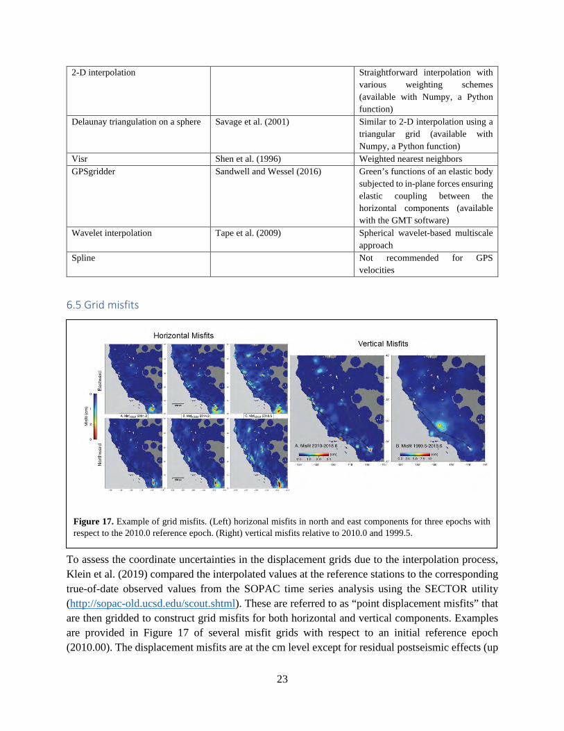
To assess the coordinate uncertainties in the displacement grids due to the interpolation process, Klein et al. (2019) compared the interpolated values at the reference stations to the corresponding true-of-date observed values from the SOPAC time series analysis using the SECTOR utility (http://sopac-old.ucsd.edu/scout.shtml). These are referred to as “point displacement misfits” that are then gridded to construct grid misfits for both horizontal and vertical components. Examples are provided in Figure 17 of several misfit grids with respect to an initial reference epoch (2010.00). The displacement misfits are at the cm level except for residual postseismic effects (up

Figure 17. Example of grid misfits. (Left) horizonal misfits in north and east components for three epochs with respect to the 2010.0 reference epoch. (Right) vertical misfits relative to 2010.0 and 1999.5.

24

to 2-3 cm from the 2010 Mw7.2 El Mayor-Cucapah earthquake). From 2010-2018.6 there are two concentrated anomalies with misfits greater than ~ 1 cm, in northern Orange County south of Los Angeles County, which is due to a well-known area of subsidence sampled by only 1-2 stations, and in a geothermal extraction area just south of the Salton Sea sampled by a single station. For the period 1999.5 to 2018.6 there is a single large anomaly (~5 cm) in the southern portion of the Central Valley (Figure 15), where subsidence rates changed due to drought in the period 2012-2017.

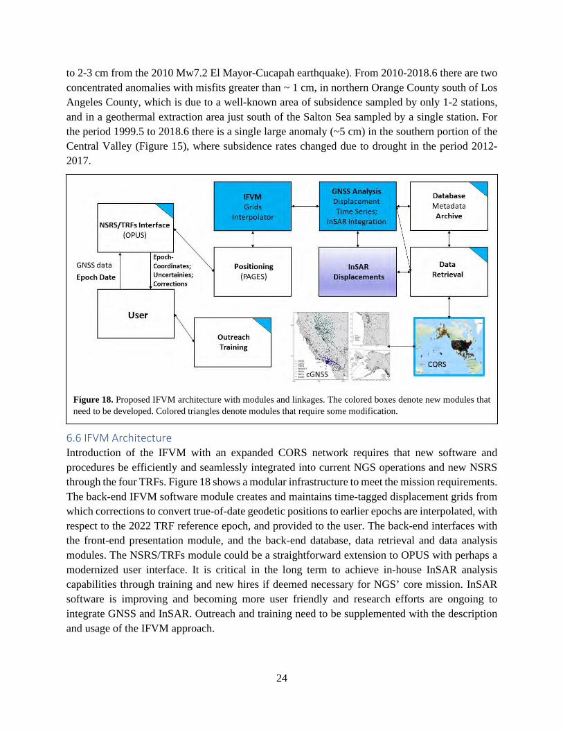
6.6 IFVM Architecture Introduction of the IFVM with an expanded CORS network requires that new software and procedures be efficiently and seamlessly integrated into current NGS operations and new NSRS through the four TRFs. Figure 18 shows a modular infrastructure to meet the mission requirements. The back-end IFVM software module creates and maintains time-tagged displacement grids from which corrections to convert true-of-date geodetic positions to earlier epochs are interpolated, with respect to the 2022 TRF reference epoch, and provided to the user. The back-end interfaces with the front-end presentation module, and the back-end database, data retrieval and data analysis modules. The NSRS/TRFs module could be a straightforward extension to OPUS with perhaps a modernized user interface. It is critical in the long term to achieve in-house InSAR analysis capabilities through training and new hires if deemed necessary for NGS’ core mission. InSAR software is improving and becoming more user friendly and research efforts are ongoing to integrate GNSS and InSAR. Outreach and training need to be supplemented with the description and usage of the IFVM approach.

Figure 18. Proposed IFVM architecture with modules and linkages. The colored boxes denote new modules that need to be developed. Colored triangles denote modules that require some modification.

25

It is critical to re-train, redirect or hire individuals to be able to maintain the IFVM, in house, to ensure the viability of the NGS effort into the long term. It would be prudent to have a contractor develop the underlying IFVM analysis software and interfaces. This would require a team of geodesists well versed in geophysical principles and reference frames, programmers, as well as NGS personnel to contribute to and oversee the process. A good idea would be to train one or more staff members perhaps through a 1-2-year Master of Science degree at a geophysics department with a strong geodetic program. For example, a thesis project could be focused on some aspect of kinematic reference frames and the individual could participate in the team that develops the software. Considering the relatively short time span until release of the new TRFs, it may be simpler to draw from the existing staff at NGS, or rely on new hires. In any case, an IFVM software package needs to be developed that can eventually be maintained and efficiently operated.

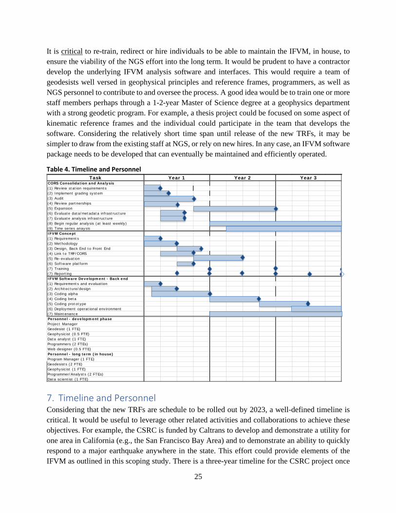
Table 4. Timeline and Personnel

7. Timeline and Personnel Considering that the new TRFs are schedule to be rolled out by 2023, a well-defined timeline is critical. It would be useful to leverage other related activities and collaborations to achieve these objectives. For example, the CSRC is funded by Caltrans to develop and demonstrate a utility for one area in California (e.g., the San Francisco Bay Area) and to demonstrate an ability to quickly respond to a major earthquake anywhere in the state. This effort could provide elements of the IFVM as outlined in this scoping study. There is a three-year timeline for the CSRC project once

TaskCORS Consolidation and Analysis(1) Review station requirements(2) Implement grading system(3) Audit(4) Review partnerships(5) Expansion(6) Evaluate data/metadata infrastructure (7) Evaluate analysis infrastructure(8) Begin regular analysis (at least weekly)(9) Time series anaysisIFVM Concept(1) Requirements(2) Methodology(3) Design, Back End to Front End(4) Link to TRF/CORS(5) Re-evaluation(6) Software platform(7) Training(7) ReportingIFVM Software Development - Back end(1) Requirements and evaluation (2) Architecture/design(3) Coding alpha(4) Coding beta(5) Coding prototype(6) Deployment operational environment(7) MaintenancePersonnel - development phaseProject ManagerGeodesist (1 FTE)Geophysicist (0.5 FTE)Data analyst (1 FTE)Programmers (2 FTEs) Web designer (0.5 FTE)Personnel - long term (in house)Program Manager (1 FTE)Geodesists (2 FTE)Geophysicist (1 FTE)Programmer/Analysts (2 FTEs)Data scientist (1 FTE)

Year 1 Year 2 Year 3

26

the contract is finalized that fits in with the new NSRS rollout schedule. If this path is chosen, it is important that someone from NGS or representing NGS be part of this effort to ensure that it would be well integrated into the NGS workflow.

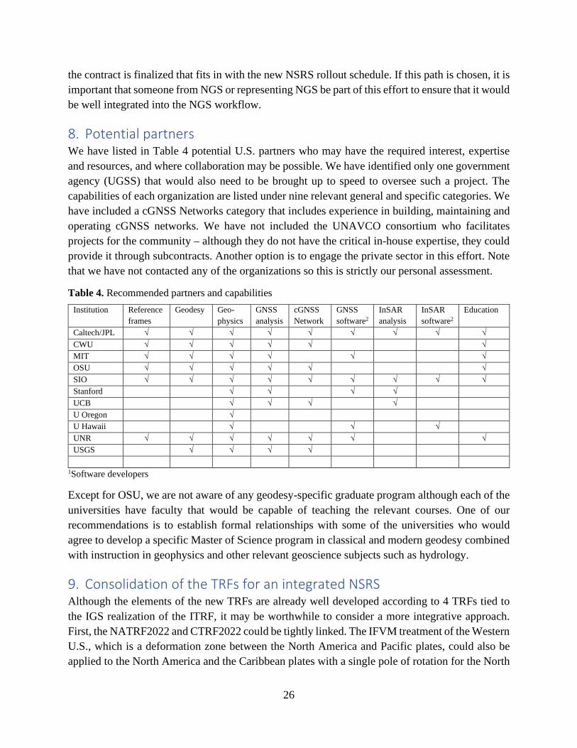
8. Potential partners We have listed in Table 4 potential U.S. partners who may have the required interest, expertise and resources, and where collaboration may be possible. We have identified only one government agency (UGSS) that would also need to be brought up to speed to oversee such a project. The capabilities of each organization are listed under nine relevant general and specific categories. We have included a cGNSS Networks category that includes experience in building, maintaining and operating cGNSS networks. We have not included the UNAVCO consortium who facilitates projects for the community – although they do not have the critical in-house expertise, they could provide it through subcontracts. Another option is to engage the private sector in this effort. Note that we have not contacted any of the organizations so this is strictly our personal assessment.

Table 4. Recommended partners and capabilities Institution Reference

frames Geodesy Geo-

physics GNSS analysis

cGNSS Network

GNSS software2

InSAR analysis

InSAR software2

Education

Caltech/JPL √ √ √ √ √ √ √ √ √ CWU √ √ √ √ √ √ MIT √ √ √ √ √ √ OSU √ √ √ √ √ √ SIO √ √ √ √ √ √ √ √ √ Stanford √ √ √ √ UCB √ √ √ √ U Oregon √ U Hawaii √ √ √ UNR √ √ √ √ √ √ √ USGS √ √ √ √

1Software developers

Except for OSU, we are not aware of any geodesy-specific graduate program although each of the universities have faculty that would be capable of teaching the relevant courses. One of our recommendations is to establish formal relationships with some of the universities who would agree to develop a specific Master of Science program in classical and modern geodesy combined with instruction in geophysics and other relevant geoscience subjects such as hydrology.

9. Consolidation of the TRFs for an integrated NSRS Although the elements of the new TRFs are already well developed according to 4 TRFs tied to the IGS realization of the ITRF, it may be worthwhile to consider a more integrative approach. First, the NATRF2022 and CTRF2022 could be tightly linked. The IFVM treatment of the Western U.S., which is a deformation zone between the North America and Pacific plates, could also be applied to the North America and the Caribbean plates with a single pole of rotation for the North

27

America craton. We suggest that NGS consider this approach rather than introducing the new CTRF2022. The two other frames PTRF2022 and MTRF2022 require special treatment since the land mass covered includes island archipelagos within the vast Pacific Rim, all in areas of active deformation and large and frequent earthquakes. Here another pole of rotation corresponding closely to the Pacific plate also aligned with IGS/ITRF may be most appropriate. Each island or island chain would only need several stations to serve as TRF base stations for local positioning needs. We realize this TRF consolidation may not be possible. However, staying with the 4 TRF's would require a duplication of efforts at differing levels and perhaps require more NGS resources and may cause some confusion among users.

28

10. References Argus, D. F., Fu, Y., & Landerer, F. W. (2014). Seasonal variation in total water storage in California inferred from GPS observations of vertical land motion. Geophysical Research Letters, 41, 1971–1980. https://doi.org/10.1002/2014GL059570

Argus, D. F., Landerer, F. W., Wiese, D. N., Martens, H. R., Fu, Y., Famiglietti, J. S., et al. (2017). Sustained water loss in California's mountain ranges during severe drought from 2012 to 2015 inferred from GPS. Journal of Geophysical Research: Solid Earth, 122, 10,559–10,585. https://doi.org/10.1002/2017JB014424

Bock, Y. & D. Melgar (2016). Physical Applications of GPS Geodesy: A Review, Rep. Prog. Phys. 79, 10, doi:10.1088/0034-4885/79/10/106801.

Bock, Y., P. Fang & G. R. Helmer (2018). California Spatial Reference System: CSRS Epoch 2017.50 (NAD83), Final report to California Department of Transportation (Caltrans), January 4.

Bock, Y. & E. Klein (2018), Investigations into a Dynamic Datum for California, Final report to California Department of Transportation (Caltrans), June 22. http://sopac-csrc.ucsd.edu/wp-content/uploads/2019/12/SIOTask4Report_final.pdf

Borsa, A. A., Agnew, D. C., & Cayan, D. R. (2014). Ongoing drought‐induced uplift in the western United States. Science, 345(6204), 1587–1590. https://doi.org/10.1126/science.1260279

P. M. Bürgi & R. B. Lohman (2020). Impact of Forest Disturbance on InSAR Surface Displacement Time Series, IEEE Transactions on Geoscience and Remote Sensing, doi: 10.1109/TGRS.2020.2992938.

Damiani, T. (2019). The NOAA Foundation CORS Network, NGS Geospatial Summit, May 7, 2019.

Emardson, T.R., Simons, M. & Webb, F.H., 2003. Neutral atmospheric delay in interferometric synthetic aperture radar applications: Statistical description and mitigation. Journal of Geophysical Research: Solid Earth, 108(B5).

Estey, L. H., & Meertens, C. M. (1999). TEQC: the multi-purpose toolkit for GPS/GLONASS data. GPS solutions, 3(1), 42-49.

Fattahi, Heresh, Mark Simons & Piyush Agram (2017). InSAR time-series estimation of the ionospheric phase delay: An extension of the split range-spectrum technique. IEEE Transactions on Geoscience and Remote Sensing 55.10 (2017): 5984-5996.

Farr, T.G., Jones, C.E., Liu, Z., Neff, K.L., Gurrola, E.M. and Manipon, G. (2016). December. Monitoring Subsidence in California with InSAR. In AGU Fall Meeting Abstracts.

Field, E. H., Arrowsmith, R. J., Biasi, G. P., Bird, P., Dawson, T. E., Felzer, K. R., et al. (2014). Uniform California earthquake rupture forecast, version 3 (UCERF3) – The time‐independent

29

model. Bulletin of the Seismological Society of America, 104(3), 1122–1180. https://doi.org/10.1785/0120130164

Frankel, A. D., Harmsen, S. C., & Boyd, O. S. (2012). The 2008 US Geological Survey national seismic hazard models and maps for the central and eastern United States. In Recent Advances in North American Paleoseismology and Neotectonics East of the Rockies (Vol. 493, pp. 243–257). Boulder, CO: The Geological Society of America.

Freed, A. M., S. T. Ali, & R. Burgmann (2007). Evolution of stress in Southern California for the past 2000 years from coseismic, postseismic and interseismic stress changes, Geophys. J. Int., 169, 1164-1179.

Gonzalez‐Ortega, A., Fialko, Y., Sandwell, D., Fletcher, J., Gonzalez‐Garcia, J., Lipovsky, B., et al. (2014). El Mayor‐Cucapah (Mw 7.2) earthquake: Early near‐field postseismic deformation from InSAR and GPS observations. Journal of Geophysical Research: Solid Earth, 119, 1482–1497. https://doi.org/10.1002/2013JB010193.

Hilla, Stephen. A new plotting program for Windows-based TEQC users. GPS solutions 6, no. 3 (2002): 196-200.

Klein, K., Y. Bock, X. Xu, D. Sandwell, D. Golriz, P. Fang, L. Su (2019). Transient deformation in California from two decades of GPS displacements: Implications for a three-dimensional kinematic reference frame, J. Geophys. Res., DOI:10.1029/2018JB017201

Lee, D., Cho, J., Suh, Y., Hwang, J., & Yun, H. (2012). A new window-based program for quality control of GPS sensing data. Remote Sensing, 4(10), 3168-3183.

Lyons, S. N., Y. Bock & D. T. Sandwell (2002), Creep along the Imperial fault, southern California, from GPS measurements, J. Geophys. Res., 107(B10), 2249, doi:10.1029/2001JB000763.

Materna, K., S. Mohanna, L. Sandoe, N. Bartlow, R. Burgmann (2019), Interseismic strain accumulation and uplift at the Mendocino Triple Junction from geodetic datasets, poster presented at 2019 AGU Annual Meeting, San Francisco.

McCaffrey, R. (2005). Block kinematics of the Pacific–North America plate boundary in the southwestern United States from inversion of GPS, seismological, and geologic data, J. Geophys. Res., 110, B07401, doi:10.1029/2004JB003307.

Meade, B.J., and B.H. Hager (2005). Block models of crustal motion in southern California constrained by GPS measurements, J. Geophys. Res., 110, doi:10.1029/2004JB003209.

Murray, J. R., N. Bartlow, Y. Bock, J. Freymueller, W. Hammond, K. Hodgkinson, I. Johanson, A. Lopez, D. Mann, G. Mattioli, T. Melbourne, D. Mencin, E. Montgomery-Brown, M. Murray, Smalley, R., V. Thomas (2019). Regional Global Navigation Satellite System Networks for Crustal Deformation Monitoring, Seismo. Res. Lett. https://doi.org/10.1785/0220190113

30

Neely, W. R., A. A. Borsa & F. Silverii (2019), GInSAR: A cGPS Correction for Enhanced InSAR Time Series, IEEE Transactions on Geoscience and Remote Sensing, 58(1), 136-146.

Ogaja, C., & Hedfors, J. (2007). TEQC multipath metrics in MATLAB. GPS Solutions, 11(3), 215-222.

Pearson, C., & Snay, R. (2013). Introducing HTDP 3.1 to transform coordinates across time and spatial reference frames, GPS Solutions, 17: 1-15.

Plesch, A., Shaw, J. H., Benson, C., Bryant, W. A., Carena, S., Cooke, M., et al. (2007). Community fault model (CFM) for southern California. Bulletin of the Seismological Society of America, 97(6), 1793–1802. https://doi.org/10.1785/0120050211

Sandwell, D. T., & Wessel, P. (2016). Interpolation of 2‐D vector data using constraints from elasticity. Geophysical Research Letters, 43(20), 10-703.

Savage, J. C., & Burford, R. (1973). Geodetic determination of relative plate motion in central California. Journal of Geophysical Research, 78, 832–845.

Savage, J. C., Gan, W., & Svarc, J. L. (2001). Strain accumulation and rotation in the Eastern California Shear Zone. Journal of Geophysical Research: Solid Earth, 106(B10), 21995-22007.

Shen, Z. K., Jackson, D. D., & Ge, B. X. (1996). Crustal deformation across and beyond the Los Angeles basin from geodetic measurements. Journal of Geophysical Research: Solid Earth, 101(B12), 27957-27980.

Smith, D., D. Roman & S. Hilla (2017). NOAA Technical Report NOS NGS 62, National Geodetic Survey, April 21.

Snay, R. A., Saleh, J., & Pearson, C. F. (2018), Improving TRANS4Ds model for vertical crustal velocities in Western CONUS, Journal of Applied Geodesy, 12: 209-27.

Tape, C., Musé, P., Simons, M., Dong, D., Webb, F. (2009). Multiscale estimation of GPS velocity fields. Geophysical Journal International, 179(2), 945-971.

Tong, X., Sandwell, D. T., & Smith‐Konter, B. (2013). High‐resolution interseismic velocity data along the San Andreas Fault from GPS and InSAR. Journal of Geophysical Research: Solid Earth, 118, 369–389. https://doi.org/10.1029/2012JB009442

Tong, X., Smith‐Konter, B., & Sandwell, D. T. (2014). Is there a discrepancy between geological and geodetic slip rates along the San Andreas Fault System? Journal of Geophysical Research: Solid Earth, 119, 2518–2538. https://doi.org/10.1002/2013JB010765

UCERF3 (2011). Report on April 2010 Workshop on Incorporating Geodetic Surface Deformation Data into UCERF3, version 3.0, 21 May.

31

Weiss, J.R., Wright, T.J., Hooper, A.J., Spaans, K., Greenall, N., Walters, R.J., González, P.J., Li, Z., Yu, C., Shen, L., Parsons, B., 2018, December. Towards large-scale, InSAR-derived surface velocities and strain rates for the global tectonic belts. In AGU Fall Meeting Abstracts.

Xu X, Sandwell DT, Klein E, Fang P, Bock Y. (2019). Line-of-Sight Deformation Time-series along the San Andreas Fault System from Sentinel-1 InSAR and GPS. AGUFM. 2019 Dec;2019:G22A-05.

Xu, X., Sandwell, D.T., Tymofyeyeva, E., Gonzalez-Ortega, A., Tong, X. (2017). Tectonic and anthropogenic deformation at the Cerro Prieto geothermal step-over revealed by Sentinel-1A InSAR. IEEE Transactions on Geoscience and Remote Sensing, 55(9), pp.5284-5292.

Xu, X. and Sandwell, D.T. (2019). Toward Absolute Phase Change Recovery With InSAR: Correcting for Earth Tides and Phase Unwrapping Ambiguities. IEEE Transactions on Geoscience and Remote Sensing.