Simulation study to inform the design ofwildcat camera trap monitoring protocols

Scottish Natural Heritage Commissioned Report No. 899

C O M M I S S I O N E D R E P O R T

Commissioned Report No. 899

Simulation study to inform the design of

wildcat camera trap monitoring protocols

For further information on this report please contact:

Jenny Bryce Scottish Natural Heritage Great Glen House Leachkin Road INVERNESS IV3 8NW Telephone: 01463 725000 E-mail: jenny.bryce@snh.gov.uk

This report should be quoted as: Newey, S., Potts, J. & Irvine, R.J. 2015. Simulation study to inform the design of wildcat camera trap monitoring protocols. Scottish Natural Heritage Commissioned Report No. 899.

This report, or any part of it, should not be reproduced without the permission of Scottish Natural Heritage. This permission will not be withheld unreasonably. The views expressed by the author(s) of this report should not be taken as the views and policies of Scottish Natural Heritage.

© Scottish Natural Heritage 2015.

i

Simulation study to inform the design of wildcat camera trap monitoring protocols

Commissioned Report No. 899 Project No: 14589 Contractor: The James Hutton Institute Year of publication: 2015 Keywords

Wild cat; Felis silvestris; wild cat action plan; camera trap; survey design. Background

The Scottish Wildcat Conservation Action Plan aims to halt the decline in Scottish wildcat numbers and to implement actions focussed on improving the conservation status of the Wildcat in Scotland. Key to assessing the outcome of conservation actions is the need monitor wildcat populations in prioritised areas. Camera trapping to collect images and identify individual wildcats for capture-recapture analysis to obtain density estimates has been proposed as the main method for monitor wildcat populations and to assess conservation measures. Here we assess, through a simulation based study, the probable effectiveness of different camera trap survey designs for monitoring wildcat population densities in designated priority areas. Main findings

Based on current knowledge of wildcat ecology we assessed how: 1) survey design; (a) number of camera traps (81, 100, 125), (b) trap spacing (750, 1,000, 1,250), and (c) survey duration (60 and 80 days), and 2) wildcat ecology; (a) population density (D=1km-2), (b) capture probability (g0=0.01, 0.02), and (c) home range (sigma = 300, 500, 700 m) affect the statistical power to detect a 25% change in wildcat density over 5 years with 80% power.

Based on the knowledge of wildcat ecology available at the time work was carried out simulations showed that; a) the number of individuals caught and recaptured tended to increase with size of trap grid, camera spacing and sigma (representing home range size), b) the number of individuals caught and recaptured also increased with survey duration and capture probability, and c) for any given grid size, sigma, capture probability and survey duration, the number of spatial recaptures (individuals caught at different locations) decreased with increasing trap spacing.

Simulations here were limited to surveys where the assumed wildcat cat density was 1km-2 which is much higher than most reported densities for wildcat populations in Scotland, but simulations using lower densities failed to run due to too few encounters.

The performance of density estimates assessed by the relative bias, relative standard error, and coverage were generally poor for surveys based on small trap grids when

COMMISSIONED REPORT

Summary

ii

sigma was small and when capture probability was low with correspondingly low poor statistical power to detect the required level of change.

The performance of density estimates increased with number of traps, capture probability, survey duration and increasing sigma with correspondingly improved statistical power.

The power to detect decreases in density was greater than to detect an increase, and in both cases statistical power was highly dependent on the combination of survey and ecological parameters.

The power of simulated survey designs increased markedly with increasing sigma. Where sigma was 300 m none of the survey designs had sufficient power (>80%) to detect the required 25% change in population density. However, when sigma was 700 m, surveys with larger camera trap grids and/or longer survey duration and when detection probability was 0.02 had sufficient power to detect a decrease and, to a lesser extent, an increase in population density.

For any given combination of sigma, detection probability larger camera trap grids and more camera traps increased power, as did longer survey duration. Similarly, for any given combination of camera trap grid, sigma, and survey duration, higher power was associated with the higher value of detection probability.

Sufficient statistical power to detect the required level of increase in wildcat density was limited to the trap grids with trap grid with 132 camera traps, where trap spacing was 1,250 m, and where sigma = 700 m. However, the utility of camera trapping to monitor wildcat density is dependent on the assumptions surveyors are prepared to make about wildcat ecology particularly home-range, but also probability of capture and probable density. New information emerging on wildcat ecology in Scotland may offer new data to inform camera trap survey studies.

For further information on this project contact: Jenny Bryce, Scottish Natural Heritage, Great Glen House, Inverness, IV3 8NW.

Tel: 01463 725000 or jenny.bryce@snh.gov.uk For further information on the SNH Research & Technical Support Programme contact:

Knowledge & Information Unit, Scottish Natural Heritage, Great Glen House, Inverness, IV3 8NW. Tel: 01463 725000 or research@snh.gov.uk

iii

Table of Contents Page

1.  INTRODUCTION 1 1.1  Background to Capture-Recapture Study Design 1 1.2  Aims & Scope 1 

2.  METHODS 2 2.1  Survey design parameters 2 2.2  Aspects of wildcat ecology 3 2.3  Simulations 4 2.4  Power analysis 6 

3.  RESULTS 6 3.1  Number of captures, recaptures and spatial recaptures 6 3.2  Bias, precision and coverage 10 3.3  Statistical power to detect change in population density 14 

4.  DISCUSSION AND CONCLUSIONS 17 4.1  Conclusions 19 

5.  REFERENCES 20 

ANNEX 1: NEW DATA ON WILDCAT ECOLOGY 22 

1

1. INTRODUCTION

Launched in 2013 the Scottish Wildcat Conservation Action Plan aims to halt the decline in Scottish wildcat (Felis. s. silvestris) numbers and to implement actions focussed on improving the conservation status of the Wildcat in Scotland (Scottish Natural Heritage 2013). In 2014 the action plan identified six priority areas for wildcat conservation (Littlewood et al. 2014). Key to assessing the outcome of conservation actions on wildcat populations is the need monitor wildcat populations in these areas. Camera trapping combined with spatially explicit capture-recapture (SECR) methods have been successfully used to survey and monitor wildcat populations in Scotland (Hetherington & Campbell 2012; Littlewood et al. 2014; Kilshaw et al. 2014) and have been proposed as the basis for wildcat monitoring in these areas. The use of camera traps has grown enormously in recent years and camera trapping has proven particular successful for monitoring elusive animals when population density is low (Long et al. 2008; O’Connell, Nichols & Karanth 2011). However designing survey protocols that have sufficient statistical power to detect important changes in population size remains challenging. (O’Connell, Nichols & Karanth 2011). Here we assess, through a simulation based study, the probable effectiveness of different sampling regimes based on camera trapping surveys for monitoring wildcat population densities in designated priority areas using spatially explicit capture-recapture (SECR) methods. 1.1 Background to Capture-Recapture Study Design

Irrespective of the mode of “capture” two of the main considerations of any capture-recapture survey design are the spatial extent of the trap grid and the spacing between traps. The spatial extent of the trap grid is a function of both the number of traps (or detectors), and inter-trap spacing distance. While both number of traps and spacing influence the extent of the grid they also affect the number of individuals caught or detected, recaptured and spatial recaptures differently (Sollmann, Gardner & Belant 2012; Sun, Fuller & Royle 2014). Survey design has to consider the total size of the trap grid, the number of traps/detectors and the spacing of traps relative to individual movement (Sollmann, Gardner & Belant 2012). Trapping grids with a large spatial extent will increase the expected number of unique individuals captured as a large grid will cover more individual home-ranges than a small grid, and also have greater potential to capture the full range of movement of individuals, homogenize unequal detection rates among individuals, and better sample non-homogenous distributions (Sun, Fuller & Royle 2014). At the same time trap spacing influences rates of detection and recaptures, and critically for SECR methods; spatial recaptures - traps that are too widely spaced relative to home-range size may lead to individuals only being detected at one location, or if spacing causes “holes” or spacing is greater than home-range diameter, animals may not be detected at all (Sollmann, Gardner & Belant 2012; Sun, Fuller & Royle 2014). While not detecting some individuals is an inherent feature of capture-recapture studies, it is assumed that all individuals have a greater than zero probability of being captured. 1.2 Aims & Scope

Purpose: to carry out a generic (i.e. non site specific) simulation study to inform the design of wildcat camera trap monitoring protocols in the wildcat priority areas with a view to assessing population trends. Aim: To assess the ability of a range of camera trapping survey designs to assess wildcat population change using SECR informed by data collected during scoping and survey work in winter 2013/14 (Littlewood et al. 2014) with reference to the Cairngorms Wildcat Project

2

Report (Hetherington & Campbell 2012) and in discussion with Jenny Bryce (SNH) and Kerry Kilshaw (WildCRU). Key parameters for detecting population change relate to the precision of the density estimates. Camera traps and image data are used to detect and identify individual wildcats and SECR analyses uses this information to estimate population density (and the variance in these estimates) based on the number of captures (individuals), recaptures, and the number of recaptures at different locations. The key variables of interest to SNH in designing a camera trap monitoring programme are: Number of cameras on a single (flexible) grid (scaled to ideally cover all of the suitable

habitats in the wildcat action plan priority areas (Littlewood et al. 2014), Camera trap spacing (informed by capture data from previous studies), Duration of surveys (this has already been assessed (Hetherington & Campbell 2012;

Kilshaw et al. 2014), however further simulations over the range of population densities encountered during the 2013-14 scoping study (Littlewood et al. 2014) are proposed).

SNH have proposed that surveys should be capable of detecting a 25% change in population density with 80% power over 5 years. 2. METHODS

Using wildcat ecological data and the survey parameters collected during previous studies (Corbett 1979; Scott, Easterbee & Jefferies 1993; Daniels 1997; Hetherington & Campbell 2012; Kilshaw et al. 2014; Littlewood et al. 2014) we assess the effect of camera trap survey design on bias, precision, and statistical power using the R package “secrdesign” (Efford 2014). Specifically we assess how a) survey design (number of camera traps, trap spacing, and survey duration) and b) wildcat ecology (population density, capture probability and home range) affect the statistical power to detect a 25% change in wildcat density over 5 years with 80% power. 2.1 Survey design parameters

The size of a camera trapping grid depends on both the number of camera traps deployed and spacing between them.

1. Number of cameras deployed affects the spatial coverage along with required accuracy and precision, but also to a large extent invariably depends on resources to purchase equipment, deploy and visit cameras as well as manage the resulting data. Based on previous studies and the need to cover areas of between 75 – 120 km2 (7,520 – 11,994 Ha) of wildcat habitat and a notional camera spacing (see below) of 1km, three levels of camera trap number were considered here; 72 (a 9 by 8 grid), 100 (a 10 by 10 grid) and 132 (a 12 by 11) grid.

2. Camera trap spacing; camera trap studies typically aim to deploy at least one camera trap per animal home range to ensure that all animals in a study area have a greater than zero probability of encountering a camera trap. Based on the minimum home range of female Scottish wildcats of around 1.75km2 (Corbett, 1979; Daniels et al., 2001; equating to an approximate 99% home range diameter of 1.450m), Kilshaw et al. (2014) and Littlewood et al. (2014) located camera trap stations 0.8–1.5 km apart so that individuals with the smallest recorded home range had a probability of greater than zero of encountering a camera trap station. However the low capture, recapture and particularly the low recapture rate at different camera trap stations reported by Littlewood et al. (2014) who used a mean camera trap spacing of 1.2km suggests that

3

at least in those areas surveyed camera trap spacing was possibly too large (Littlewood et al., 2014). Here we therefore assess the effects of camera trap spacing of 750, 1,000, 1,250 m.

3. Survey duration required to attain sufficient captures and recaptures and to capture the majority of the resident population while maintaining “population closure” (the assumption that the population should remain closed to demographic change over the course of the survey) has been assessed by Kilshaw et al. (2014) and Hetherington & Campbell (2012) who suggest that 60 days is optimal. However, surveys of extremely low density populations may benefit from extended survey duration, we therefore assess the effect of 60 and 80 days, the maximum length considered feasible to maintain closure.

2.2 Aspects of wildcat ecology

Three ecological parameters are needed for the simulations:

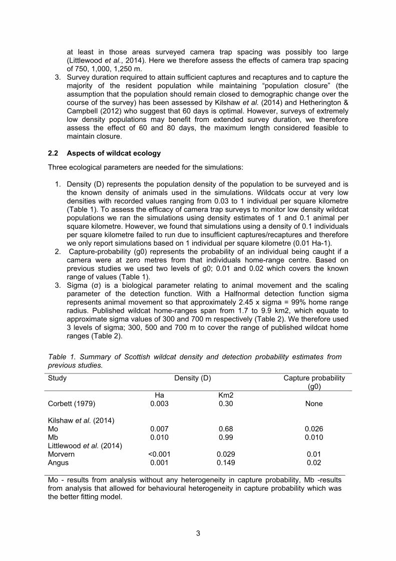
1. Density (D) represents the population density of the population to be surveyed and is the known density of animals used in the simulations. Wildcats occur at very low densities with recorded values ranging from 0.03 to 1 individual per square kilometre (Table 1). To assess the efficacy of camera trap surveys to monitor low density wildcat populations we ran the simulations using density estimates of 1 and 0.1 animal per square kilometre. However, we found that simulations using a density of 0.1 individuals per square kilometre failed to run due to insufficient captures/recaptures and therefore we only report simulations based on 1 individual per square kilometre (0.01 Ha-1).

2. Capture-probability (g0) represents the probability of an individual being caught if a camera were at zero metres from that individuals home-range centre. Based on previous studies we used two levels of g0; 0.01 and 0.02 which covers the known range of values (Table 1).

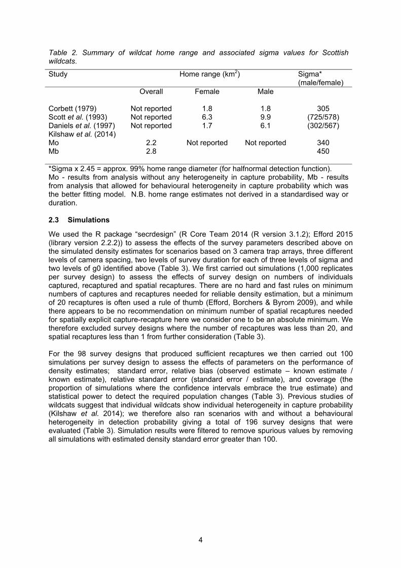
3. Sigma (σ) is a biological parameter relating to animal movement and the scaling parameter of the detection function. With a Halfnormal detection function sigma represents animal movement so that approximately 2.45 x sigma = 99% home range radius. Published wildcat home-ranges span from 1.7 to 9.9 km2, which equate to approximate sigma values of 300 and 700 m respectively (Table 2). We therefore used 3 levels of sigma; 300, 500 and 700 m to cover the range of published wildcat home ranges (Table 2).

Table 1. Summary of Scottish wildcat density and detection probability estimates from previous studies.

Study Density (D) Capture probability (g0)

Ha Km2 Corbett (1979) 0.003 0.30 None Kilshaw et al. (2014) Mo Mb

0.007 0.010

0.68 0.99

0.026 0.010

Littlewood et al. (2014) Morvern Angus

<0.001 0.001

0.029 0.149

0.01 0.02

Mo - results from analysis without any heterogeneity in capture probability, Mb -results from analysis that allowed for behavioural heterogeneity in capture probability which was the better fitting model.

4

Table 2. Summary of wildcat home range and associated sigma values for Scottish wildcats.

Study Home range (km2) Sigma* (male/female)

Overall Female Male Corbett (1979) Not reported 1.8 1.8 305 Scott et al. (1993) Not reported 6.3 9.9 (725/578) Daniels et al. (1997) Not reported 1.7 6.1 (302/567) Kilshaw et al. (2014) Mo Mb

2.2 2.8

Not reported

Not reported

340 450

*Sigma x 2.45 = approx. 99% home range diameter (for halfnormal detection function). Mo - results from analysis without any heterogeneity in capture probability, Mb - results from analysis that allowed for behavioural heterogeneity in capture probability which was the better fitting model. N.B. home range estimates not derived in a standardised way or duration. 2.3 Simulations

We used the R package “secrdesign” (R Core Team 2014 (R version 3.1.2); Efford 2015 (library version 2.2.2)) to assess the effects of the survey parameters described above on the simulated density estimates for scenarios based on 3 camera trap arrays, three different levels of camera spacing, two levels of survey duration for each of three levels of sigma and two levels of g0 identified above (Table 3). We first carried out simulations (1,000 replicates per survey design) to assess the effects of survey design on numbers of individuals captured, recaptured and spatial recaptures. There are no hard and fast rules on minimum numbers of captures and recaptures needed for reliable density estimation, but a minimum of 20 recaptures is often used a rule of thumb (Efford, Borchers & Byrom 2009), and while there appears to be no recommendation on minimum number of spatial recaptures needed for spatially explicit capture-recapture here we consider one to be an absolute minimum. We therefore excluded survey designs where the number of recaptures was less than 20, and spatial recaptures less than 1 from further consideration (Table 3). For the 98 survey designs that produced sufficient recaptures we then carried out 100 simulations per survey design to assess the effects of parameters on the performance of density estimates; standard error, relative bias (observed estimate – known estimate / known estimate), relative standard error (standard error / estimate), and coverage (the proportion of simulations where the confidence intervals embrace the true estimate) and statistical power to detect the required population changes (Table 3). Previous studies of wildcats suggest that individual wildcats show individual heterogeneity in capture probability (Kilshaw et al. 2014); we therefore also ran scenarios with and without a behavioural heterogeneity in detection probability giving a total of 196 survey designs that were evaluated (Table 3). Simulation results were filtered to remove spurious values by removing all simulations with estimated density standard error greater than 100.

5

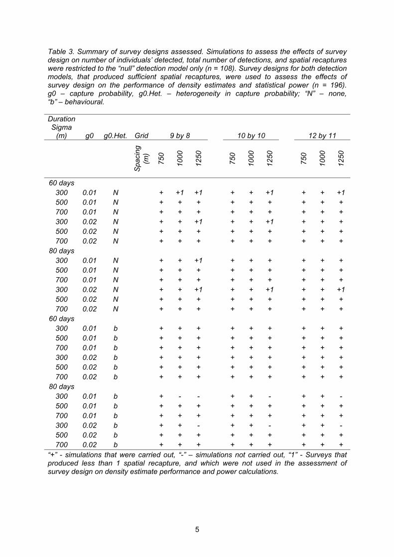
Table 3. Summary of survey designs assessed. Simulations to assess the effects of survey design on number of individuals’ detected, total number of detections, and spatial recaptures were restricted to the “null” detection model only (n = 108). Survey designs for both detection models, that produced sufficient spatial recaptures, were used to assess the effects of survey design on the performance of density estimates and statistical power (n = 196). g0 – capture probability, g0.Het. – heterogeneity in capture probability; “N” – none, “b” – behavioural. Duration Sigma

(m) g0 g0.Het. Grid 9 by 8 10 by 10

12 by 11

Spa

cing

(m

)

750

1000

1250

750

1000

1250

750

1000

1250

60 days 300 0.01 N + +1 +1 + + +1 + + +1 500 0.01 N + + + + + + + + + 700 0.01 N + + + + + + + + + 300 0.02 N + + +1 + + +1 + + + 500 0.02 N + + + + + + + + + 700 0.02 N + + + + + + + + +

80 days 300 0.01 N + + +1 + + + + + + 500 0.01 N + + + + + + + + + 700 0.01 N + + + + + + + + + 300 0.02 N + + +1 + + +1 + + +1 500 0.02 N + + + + + + + + + 700 0.02 N + + + + + + + + +

60 days 300 0.01 b + + + + + + + + + 500 0.01 b + + + + + + + + + 700 0.01 b + + + + + + + + + 300 0.02 b + + + + + + + + + 500 0.02 b + + + + + + + + + 700 0.02 b + + + + + + + + +

80 days 300 0.01 b + - - + + - + + - 500 0.01 b + + + + + + + + + 700 0.01 b + + + + + + + + + 300 0.02 b + + - + + - + + - 500 0.02 b + + + + + + + + + 700 0.02 b + + + + + + + + +

“+” - simulations that were carried out, “-” – simulations not carried out, “1” - Surveys that produced less than 1 spatial recapture, and which were not used in the assessment of survey design on density estimate performance and power calculations.

6

2.4 Power analysis

The estimated mean and upper and lower confidence limits for the density predictions for each survey design were log-transformed. As the 95% confidence interval for a standard normal distribution corresponds to approximately 1.96 standard deviations either side of the mean, the standard error on the log scale was estimated by dividing the difference between the upper and lower confidence limits by 2×1.96. The power to detect a change in the population, assuming a 25% decrease and a 25% increase in the population was then calculated. This was done by calculating the probability that a value drawn from a normal distribution lies outside the log-transformed confidence limits. In the case of a 25% decrease, the mean of the distribution was taken as the log-transformed mean + log(0.75) and in the case of a 25% increase it was taken as the log-transformed mean + log(1.25), and the standard deviation was assumed to remain equal to the estimated standard error on the log scale. Due to the asymmetric nature of the confidence intervals the power to detect a 25% increase in the population is lower than the power to detect a 25% decrease in each case. A power of 0.8 or greater is generally considered acceptable. 3. RESULTS

3.1 Number of captures, recaptures and spatial recaptures

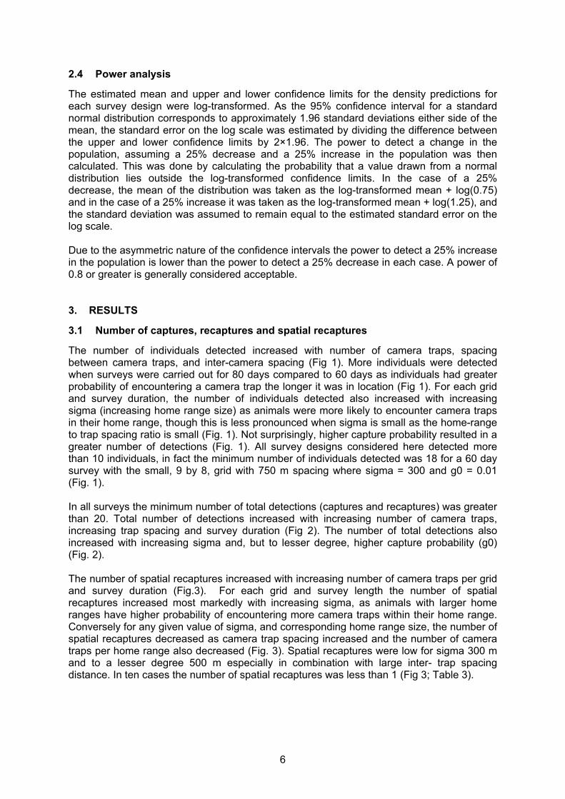
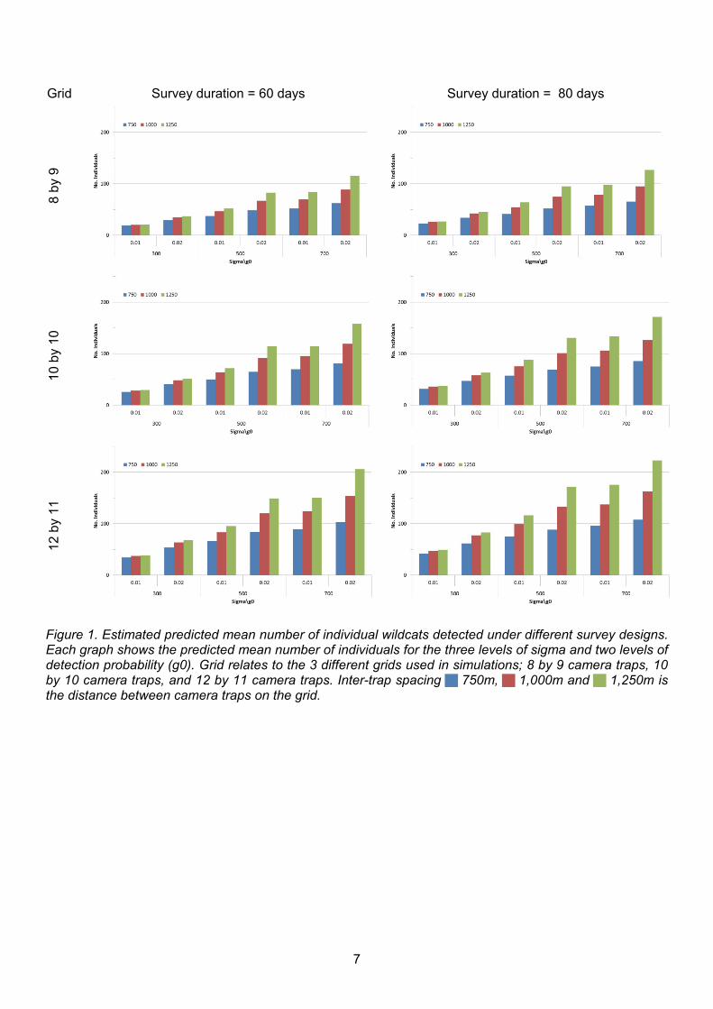
The number of individuals detected increased with number of camera traps, spacing between camera traps, and inter-camera spacing (Fig 1). More individuals were detected when surveys were carried out for 80 days compared to 60 days as individuals had greater probability of encountering a camera trap the longer it was in location (Fig 1). For each grid and survey duration, the number of individuals detected also increased with increasing sigma (increasing home range size) as animals were more likely to encounter camera traps in their home range, though this is less pronounced when sigma is small as the home-range to trap spacing ratio is small (Fig. 1). Not surprisingly, higher capture probability resulted in a greater number of detections (Fig. 1). All survey designs considered here detected more than 10 individuals, in fact the minimum number of individuals detected was 18 for a 60 day survey with the small, 9 by 8, grid with 750 m spacing where sigma = 300 and g0 = 0.01 (Fig. 1). In all surveys the minimum number of total detections (captures and recaptures) was greater than 20. Total number of detections increased with increasing number of camera traps, increasing trap spacing and survey duration (Fig 2). The number of total detections also increased with increasing sigma and, but to lesser degree, higher capture probability (g0) (Fig. 2). The number of spatial recaptures increased with increasing number of camera traps per grid and survey duration (Fig.3). For each grid and survey length the number of spatial recaptures increased most markedly with increasing sigma, as animals with larger home ranges have higher probability of encountering more camera traps within their home range. Conversely for any given value of sigma, and corresponding home range size, the number of spatial recaptures decreased as camera trap spacing increased and the number of camera traps per home range also decreased (Fig. 3). Spatial recaptures were low for sigma 300 m and to a lesser degree 500 m especially in combination with large inter- trap spacing distance. In ten cases the number of spatial recaptures was less than 1 (Fig 3; Table 3).

7

Grid Survey duration = 60 days Survey duration = 80 days

8 by

9

10 b

y 10

12

by

11

     Figure 1. Estimated predicted mean number of individual wildcats detected under different survey designs. Each graph shows the predicted mean number of individuals for the three levels of sigma and two levels of detection probability (g0). Grid relates to the 3 different grids used in simulations; 8 by 9 camera traps, 10 by 10 camera traps, and 12 by 11 camera traps. Inter-trap spacing  750m,  1,000m and  1,250m is the distance between camera traps on the grid.

8

Grid Survey duration = 60 days Survey duration = 80 days

8 by

9

10 b

y 10

12

by

11

     Figure 2. Estimated predicted mean total number of detections under different survey designs. Each graph shows the mean predicted number of detections for three levels of sigma and two levels of detection probability (g0. Grid relates to the 3 different grids used in simulations; 8 by 9 camera traps, 10 by 10 camera traps, and 12 by 11 camera traps. Inter-trap spacing  750m,  1,000m and  1,250m is the distance between camera traps on the grid.

9

Grid Survey duration = 60 days Survey duration = 80 days

8 by

9

10 b

y 10

12

by

11

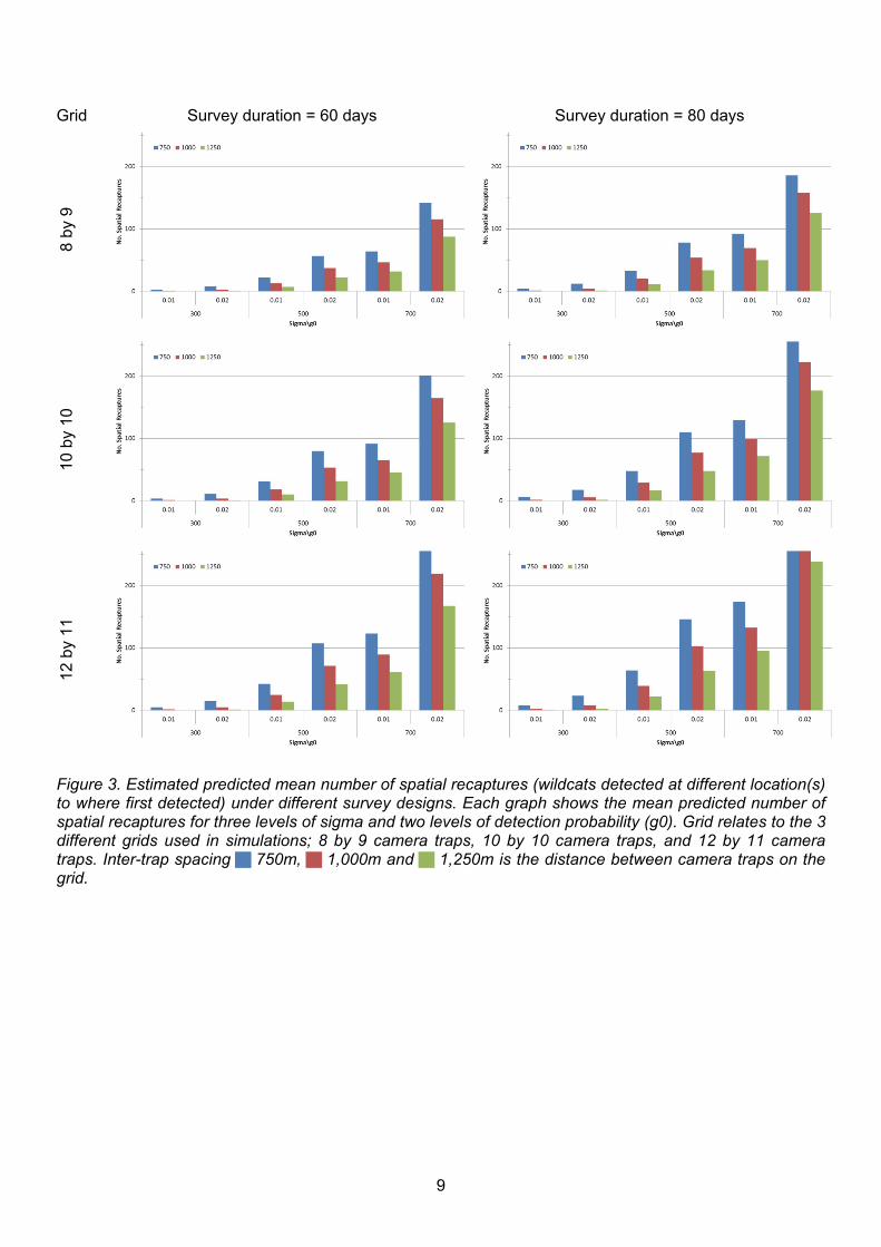
     Figure 3. Estimated predicted mean number of spatial recaptures (wildcats detected at different location(s) to where first detected) under different survey designs. Each graph shows the mean predicted number of spatial recaptures for three levels of sigma and two levels of detection probability (g0). Grid relates to the 3 different grids used in simulations; 8 by 9 camera traps, 10 by 10 camera traps, and 12 by 11 camera traps. Inter-trap spacing  750m,  1,000m and  1,250m is the distance between camera traps on the grid. 

10

3.2 Bias, precision and coverage

Focusing on the 98 survey designs that the previous results suggested would give sufficient data for SECR analysis, we considered how survey design influenced performance of density estimates with and without behavioural heterogeneity in detection probability. Relative bias (%RB) and relative standard error (%RSE) showed very similar patterns. Surveys with the two lower sigma values, particularly when combined with low detection probability and behavioural heterogeneity in detection, show high %RB and %RSE (Fig. 4, Table 4). Performance of density estimates improved (i.e. lower %RB and %RSE) with increasing number of camera traps. Survey duration was also important with 80 day surveys performing better than 60 day surveys as animals had greater probability of encountering camera traps (Fig. 4, Table 4). The effects of camera trap spacing were not as clear and, as was shown by numbers of spatial recaptures (Fig. 4), interacted with sigma; small values of sigma and larger inter-camera trap distances combined to produce higher %RB and %RSE. Low detection probability and heterogeneity in detection probability lead to higher %RB and %RSE (Fig. 4, Table 4). For those survey designs considered here, percentage coverage (%COV; the percentage of simulations where the true density lies within the estimated confidence intervals) is generally good, with the lowest value of 80% for a 60 day survey with an 9 by 8 grid with 1,000 m inter-trap spacing where g0 = 0.01 with behavioural heterogeneity (Fig. 5). Low %COV is associated with small sigma, low capture probability and behavioural heterogeneity in capture probability (Fig. 5).

11

Grid Survey duration = 60 days Survey duration = 80 days

8 by

9

10 b

y 10

12

by

11

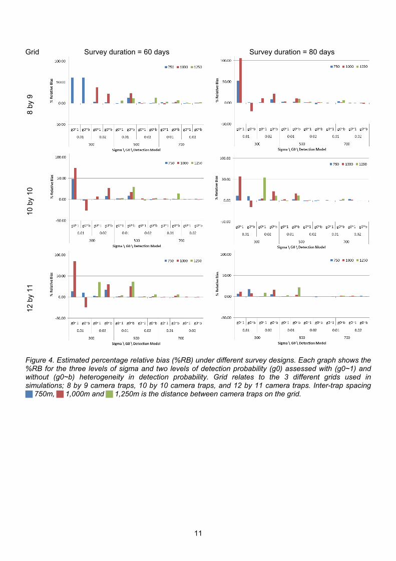
     Figure 4. Estimated percentage relative bias (%RB) under different survey designs. Each graph shows the %RB for the three levels of sigma and two levels of detection probability (g0) assessed with (g0~1) and without (g0~b) heterogeneity in detection probability. Grid relates to the 3 different grids used in simulations; 8 by 9 camera traps, 10 by 10 camera traps, and 12 by 11 camera traps. Inter-trap spacing  750m,  1,000m and  1,250m is the distance between camera traps on the grid. 

12

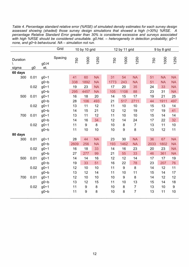
Table 4. Percentage standard relative error (%RSE) of simulated density estimates for each survey design assessed showing (shaded) those survey design simulations that showed a high (>30%) %RSE. A percentage Relative Standard Error greater than 30% is considered excessive and surveys associated with high %RSE should be considered unsuitable. g0.Het. – heterogeneity in detection probability; g0~1 none, and g0~b behavioural. NA – simulation not run. 

Grid 10 by 10 grid 12 by 11 grid 9 by 8 grid

Duration\ sigma g0

g0.Het.

Spacing

750

1000

1250

750

1000

1250

750

1000

1250

60 days 300 0.01 g0~1 41 60 NA 31 54 NA 51 NA NA

g0~b 338 1892 NA 1773 243 NA 51 NA NA 0.02 g0~1 19 23 NA 17 20 35 24 33 NA

g0~b 295 4457 NA 105 1108 88 23 31 NA 500 0.01 g0~1 16 18 20 14 15 17 19 21 25

g0~b 28 106 493 21 517 2711 44 1911 497 0.02 g0~1 13 11 12 11 10 10 15 13 14

g0~b 14 15 21 12 12 19 17 19 41 700 0.01 g0~1 13 11 12 11 10 10 15 14 14

g0~b 14 16 34 12 14 24 17 22 32 0.02 g0~1 11 9 8 10 8 7 13 11 10

g0~b 11 10 10 10 9 8 13 12 11 80 days

300 0.01 g0~1 28 44 NA 23 30 NA 36 67 NA g0~b 2609 256 NA 193 1462 NA 2033 1802 NA

0.02 g0~1 16 18 33 14 16 23 20 23 NA g0~b 27 277 99 21 55 33 46 361 NA

500 0.01 g0~1 14 14 16 12 12 14 17 17 19 g0~b 19 33 51 16 22 78 23 207 76

0.02 g0~1 12 10 10 11 9 8 14 12 11 g0~b 13 12 14 11 10 11 15 14 17

700 0.01 g0~1 12 10 10 10 9 8 14 12 12 g0~b 13 12 15 11 10 13 15 14 18

0.02 g0~1 11 9 8 10 8 7 13 10 9 g0~b 11 9 8 10 8 7 13 11 10

13

Grid  Survey duration = 60 days  Survey duration = 80 day 

8 by 9 

10 by 10 

12 by 11 

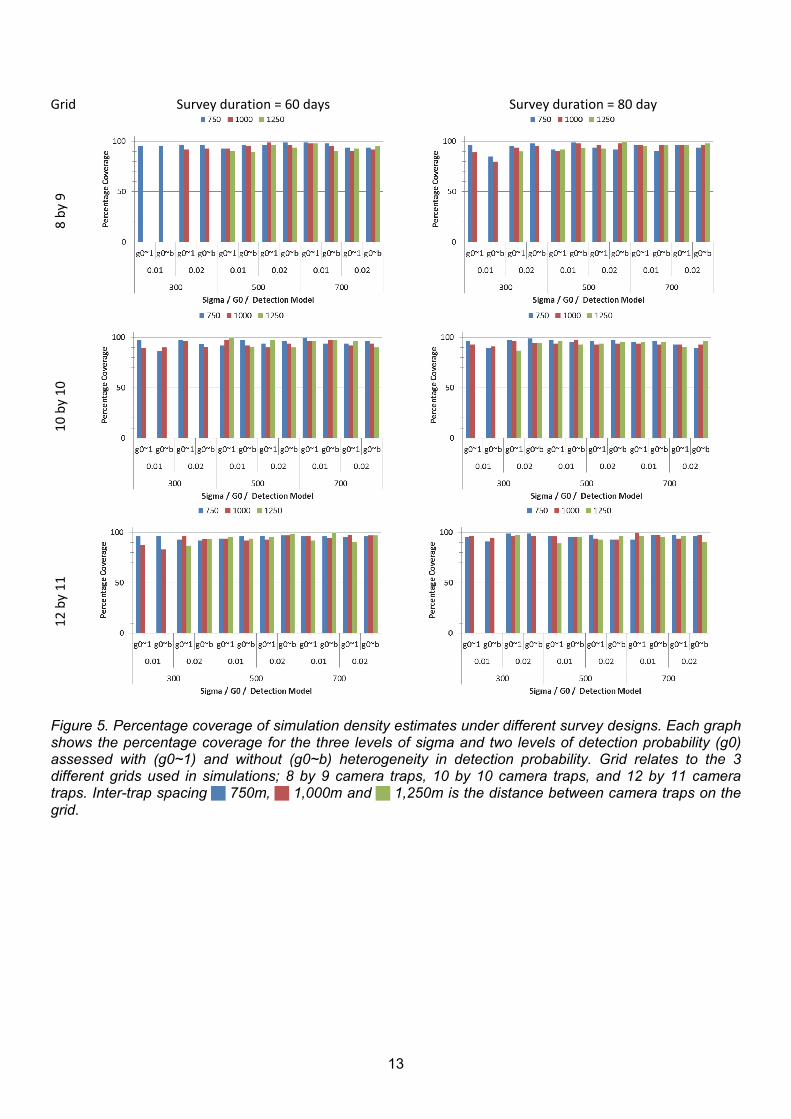
     Figure 5. Percentage coverage of simulation density estimates under different survey designs. Each graph shows the percentage coverage for the three levels of sigma and two levels of detection probability (g0) assessed with (g0~1) and without (g0~b) heterogeneity in detection probability. Grid relates to the 3 different grids used in simulations; 8 by 9 camera traps, 10 by 10 camera traps, and 12 by 11 camera traps. Inter-trap spacing  750m,  1,000m and  1,250m is the distance between camera traps on the grid. 

14

3.3 Statistical power to detect change in population density

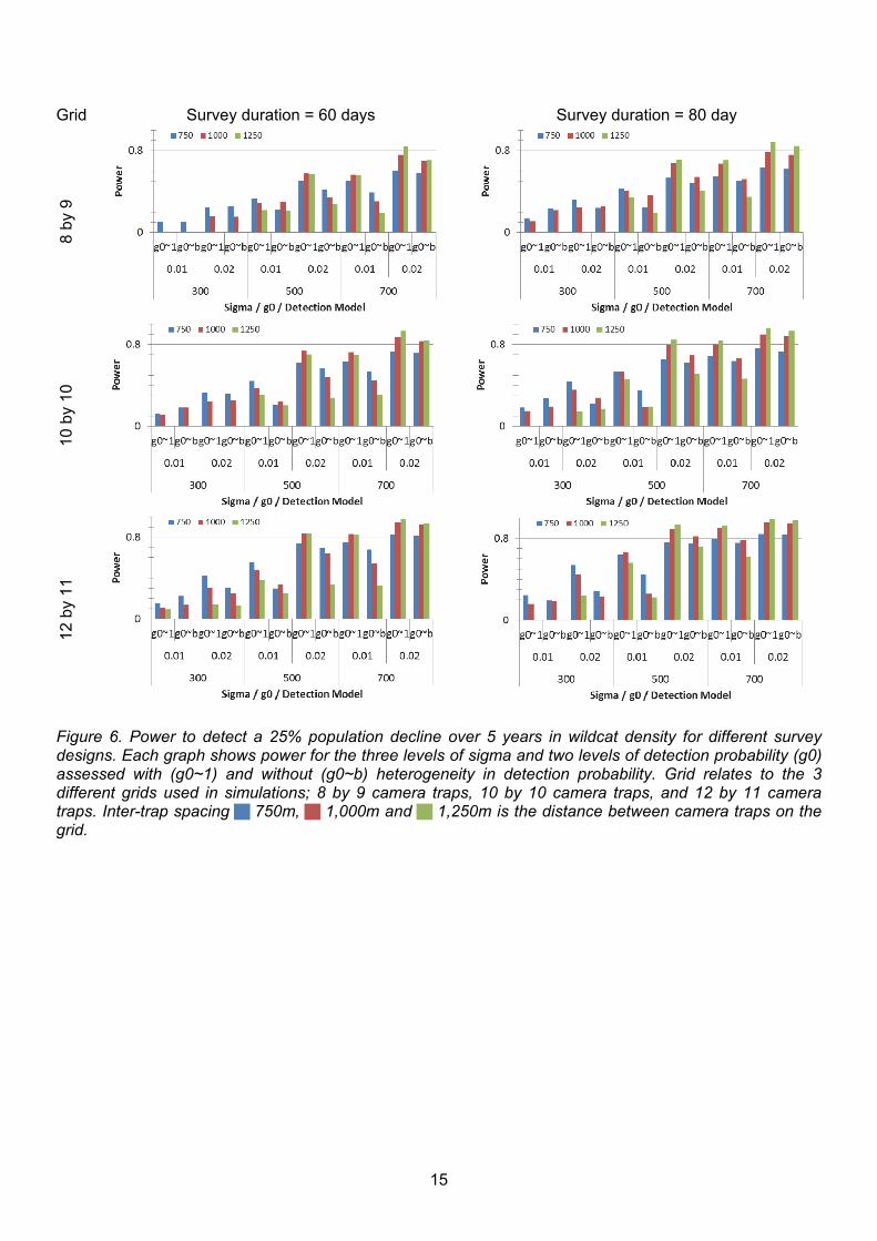
The statistical power of a particular survey design to detect either an increase or decrease was highly dependent on the combination of survey and ecological parameters. The power of simulated survey designs increased markedly with increasing sigma (Figs. 6, 7). Where sigma was 300 m none of the survey designs had sufficient power (>80%) to detect the required 25% change in population density (Figs 6, 7). However, when sigma was 700 m, surveys with larger camera trap grids and/or longer survey duration and when detection probability was 0.02 had sufficient power to detect a decrease and, to a lesser extent, an increase in population density in the absence of heterogeneity in detection probability (Figs 6, 7). At the intermediate value of sigma (= 500 m) power was strongly influenced by detection probability and heterogeneity whereby power was greater at higher detection probability and without heterogeneity (Figs. 6, 7). For any given combination of sigma, detection probability, and detection model, larger camera trap grids and more camera traps increased power, as did longer survey duration albeit to a lesser extent (Figs 6, 7). Similarly, for any given combination of camera trap grid, sigma, and survey duration, higher power was associated with the higher value of detection probability (Figs 6, 7). In most cases inclusion of behavioural heterogeneity in capture probability was associated with decreased power, but this was not consistent across all levels of sigma; when sigma equals 700 m and capture probability is 0.02, the effect on power appears small (Figs. 6, 7). The effect of camera trap spacing was also not consistent; when sigma is small increased inter-camera spacing decreases power, but this was reversed when sigma and capture probability were higher (Figs 6, 7).

15

Grid Survey duration = 60 days Survey duration = 80 day

8 by

9

10 b

y 10

12

by

11

     Figure 6. Power to detect a 25% population decline over 5 years in wildcat density for different survey designs. Each graph shows power for the three levels of sigma and two levels of detection probability (g0) assessed with (g0~1) and without (g0~b) heterogeneity in detection probability. Grid relates to the 3 different grids used in simulations; 8 by 9 camera traps, 10 by 10 camera traps, and 12 by 11 camera traps. Inter-trap spacing  750m,  1,000m and  1,250m is the distance between camera traps on the grid. 

16

Grid Survey duration = 60 days Survey duration = 80 day

8 by

9

10 b

y 10

12

by

11

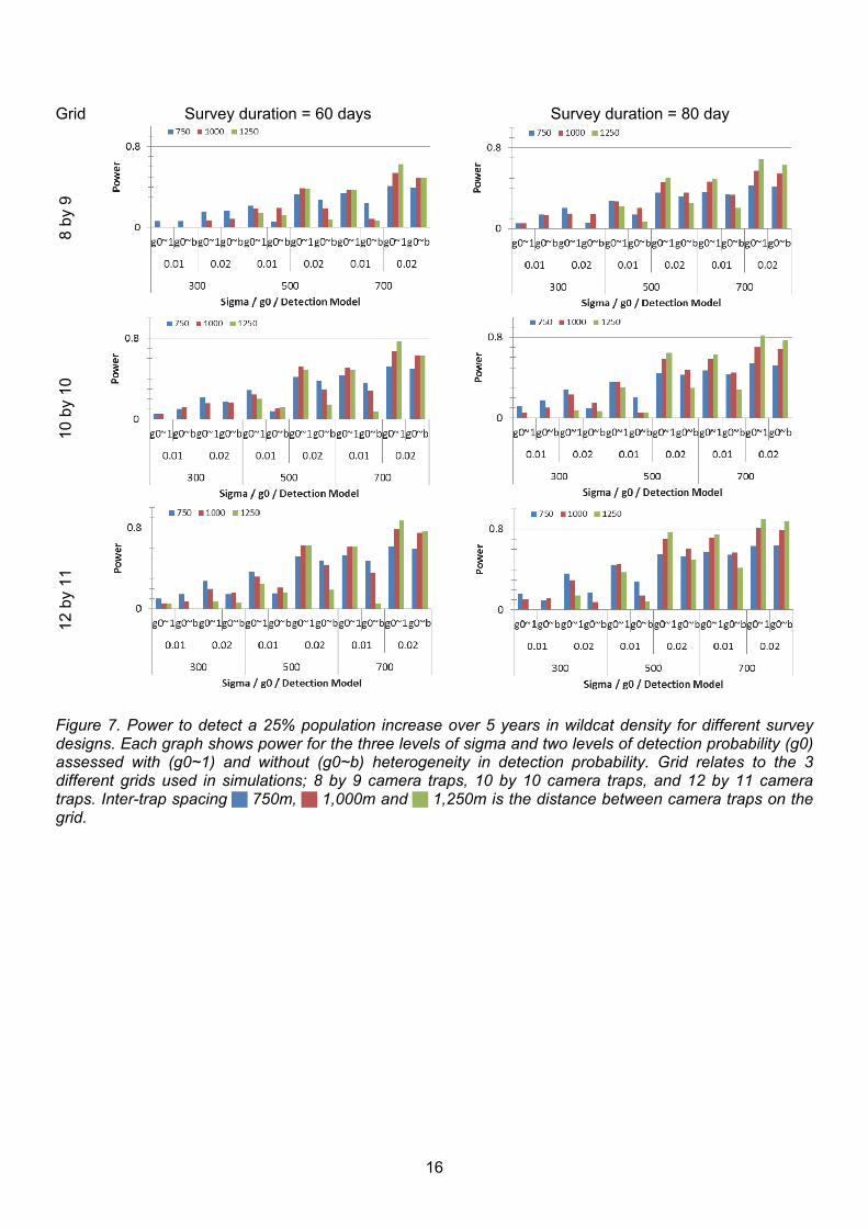
     Figure 7. Power to detect a 25% population increase over 5 years in wildcat density for different survey designs. Each graph shows power for the three levels of sigma and two levels of detection probability (g0) assessed with (g0~1) and without (g0~b) heterogeneity in detection probability. Grid relates to the 3 different grids used in simulations; 8 by 9 camera traps, 10 by 10 camera traps, and 12 by 11 camera traps. Inter-trap spacing  750m,  1,000m and  1,250m is the distance between camera traps on the grid. 

17

4. DISCUSSION AND CONCLUSIONS

The results shown by the simulations reported here are largely consistent with the few other studies that have assessed how spatial study design and trap configuration and spacing influence capture and recapture rates. Simulations show that expected capture and recapture rates increase with number of camera traps and larger trap grids, and that spatial recaptures tend to decline as inter-trap spacing increases relative to home-range. As expected more individuals were captured and recaptured when detectability is higher. Including behavioural heterogeneity in detection probability was generally associated with an increase in relative bias and relative standard error, and lower power. The reasons for this are not clear, but it is most pronounced for smaller home-ranges indicating that heterogeneity of detection is likely to have a proportionally larger effect when recapture probability and spatial recaptures rates are low. Modelling and simulation studies play an important and useful role in ecology allowing us to explore scenarios and hypotheses before embarking on labour intensive field studies. However, the results of simulations should be considered with due regard to the implicit and explicit assumptions, and modelling framework. None of the simulations here, for example, accommodate for the vagaries and challenges of Scottish weather! While many of the assumptions used in this analysis are design based and are therefore within the surveyors’ control, two key biological parameters - g0 and sigma - were estimated from a small number of previous studies and the literature. Both of these are likely to be habitat and site dependent, will vary seasonally, annually and by individual and will impact the on efficacy of live trapping/camera trap studies. Simulations here have assumed a constant and regular study area where traps can be placed in a regular grid according to the survey design. In practice, it makes sense for the camera trap placement to be limited to areas of suitable habitat and cameras should be placed in areas so as to maximise the probability of detecting wildcats and will therefore be placed in edge habitat, runs, and surveys will need to accommodate access restrictions and inaccessible areas. Survey grids will therefore almost certainly be an irregular shape, with variable trap spacing, and may compose of one or more irregular/disjointed grids. Fortunately, SECR methods easily accommodate irregular, and even separate, grids and irregular trap spacing. Indeed distributing camera traps among two or more smaller grids (clusters) may be beneficial and has been shown to be an effective design in some circumstances combining both large spatial extent and appropriate inter-trap spacing (Sollmann, Gardner & Belant 2012; Sun, Fuller & Royle 2014). However, it is important to understand how grid size and shape might affect capture and recapture rate as, for example, while a long thin trap grid may yield a higher capture rate of novel individuals compared to a square grid with the same number of traps, recapture and spatial recapture rates may be lower, similarly the same number of camera traps distributed among a number of clusters may produce more captures than the same number of camera traps placed in a regular grid, but recapture rates may be lower (Sollmann, Gardner & Belant 2012; Sun, Fuller & Royle 2014). In the simulations presented here larger trap grid size also equates to more camera traps. Deploying and maintaining more camera traps is of course logistically more demanding, but seems justified in terms of survey performance predicted by our analysis. The use of camera traps in wildlife ecology has grown enormously over the last 10-20 years and camera traps are now a mainstream tool in wildlife ecology and monitoring (O’Connell, Nichols & Karanth 2011). Camera traps are undoubtedly a powerful tool in animal ecology, but despite their widespread use most commercially available camera taps are not designed for research use, and there is a growing awareness of the limitations and challenges of using camera traps for research and monitoring that practitioners should be aware of (Meek & Pittet 2013; Hamel et al. 2013; Burton et al. 2015; Meek, Ballard & Fleming 2015). In addition to the technical and practical challenges of using camera traps when successfully

18

deployed, camera traps can generate large amounts of data with associated problems of processing, data management and analysis (e.g. Harris et al. 2010; Sundaresan, Riginos & Abelson 2011). The Scottish Wildcat Conservation Action Plan proposes that camera trap surveys be carried out over winter when wildcats are not breeding and thought to be more sedentary, and more attracted to bait. Based on previous finding reported by Kilshaw et al. (2014) 60 day surveys were considered optimal in balancing demands on resources, gathering sufficient data, and based on what is known about wildcat breeding behaviour and dispersal maintaining the population “closure”. Here extending the survey period to 80 days resulted in a small but marked increase in capture, recapture and spatial recaptures rates along with improvements in bias, precision and power. However, whether the closure assumption can be maintained with the longer survey period is unclear. Logistic demands in maintaining camera traps and managing resulting data will also increase, but cost less than deploying more camera traps. The trade-offs of using longer surveys needs to be considered in view of the survey aims, logistics and assumptions underpinning analysis of camera trap data. Information on wildcat home-range is currently limited to a few (VHF) radio-tracking studies (Corbett 1979; Scott, Easterbee & Jefferies 1993; Daniels 1997), and one camera trapping study where home-range has been inferred by SECR analysis (Kilshaw et al. 2014) (Table 2). These few studies highlight the large difference in known home-ranges of wildcats in Scotland which may show substantially different ranging behaviour in different parts of Scotland; home ranges in the west of Scotland appear to be much larger than those in the east. In addition, although wildcat ranging behaviour has not been well studied, wildcats may be expected to show seasonal, age-sex, and habitat differences in ranging behaviour. In our simulations we assumed home-range, and thus sigma, were similar for males and females over the course of the survey period, because detailed sex-specific home-range data is missing or scarce. The ranging behaviour of wildcats is an active area of discussion and research and future findings may be able to better inform survey design and decisions (Appendix 1). Results presented here are all based on simulations based on population density of 1 Km2 (0.01 Ha). This value is higher than density estimates reported from the recent survey and scoping study (Littlewood et al. 2014) who reported densities of 0.03 and 0.15 km2 for two areas surveyed using camera traps in 2013-14, and of 0.3 km2 (Corbett 1979; Kilshaw & Macdonald 2011), but consistent with the estimate of 0.9 km2 (Kilshaw et al. 2014; includes wildcats and wildcat hybrids) (Table 1). Simulations were based on D=1 Km2 as those based on lower values of D consistently failed to generate sufficient data for simulations to run to completion, and based on the results reported here would certainly have poor performance characteristics in terms of bias precision and low power to detect changes in population density. Simulations were carried out using two levels of detection probability (g0; 0.01, and 0.02) which represent the range of values reported in the only other published Scottish wildcat camera trap studies (Kilshaw et al. 2014; Littlewood et al. 2014). While these are the best available empirical estimates they are derived from only two studies of three populations and in the case of Littlewood et al. (2014) based on sparse data. Not surprisingly a higher detection probability resulted in high capture and recapture rates, reduced bias, and greater precision and power. The practical implications of this are largely dependent on what assumptions surveyors can justify; assuming the worst case scenario this will require greater resources, but may lead to better results. Capture-recapture studies assume that all individuals in the study area have constant and uniform probability of capture and any violation of this assumption must be accounted for in analysis if bias and lack of precision are to be avoided (Otis et al. 1978; White et al. 1982; Amstrup, McDonald & Manly 2005). Based on the findings of Kilshaw et al. (2014) who reported evidence of behavioural

19

heterogeneity in detection probability we ran simulations with and without behavioural heterogeneity to assess how this would affect bias, precision and power. Under most survey designs the inclusion of behavioural heterogeneity in the detection probability led to increased bias and relative standard error as well as reduced power. However, the effect was small when home range was small and on the larger grids that were surveyed for the longer duration (80 days versus 60 days). More information is really needed to understand how wildcats react to camera traps and any bait or lure that might be used to attract them and how this affects survey efficacy. 4.1 Conclusions

Based on the survey designs considered here the power to detect the required 25% change in wildcat population density is entirely dependent on the assumptions surveyors are able to make concerning the home-range of cats in the survey areas, their density and detectability. Focusing on the power to detect an increase, as this the main aim of the Scottish Wildcat Conservation Action Plan, none of the survey designs have sufficient power to detect the required change in wildcat populations that have small home ranges or exist at low densities (as seems to be the case in Scotland). Only surveys of populations with large home ranges, equating to a sigma value of around 700 m, have sufficient power to detect a 25% increase in population density and even then only under scenarios when detection probability is at the higher end of the known range of values, and if there is, as suspected, behavioural heterogeneity in detection probability, then only surveys with longer survey duration and employing a large trapping grid have sufficient power. With the exception of a 60 day survey deploying the 12 by 11 trapping grid, none of the surveys deploying the small, 8 by 8, or medium 10 by 10, grids yield sufficient power. To successfully monitor and confidently detect change in wildcat populations characterised by small home-ranges as may occur in areas of greater food availability or quality, different survey designs employing smaller inter-trap distances may need to be explored. The published literature suggests that survey designs where trap spacing is no more than 2 x sigma, but not less than 0.5 sigma may work best (Sollmann, Gardner & Belant 2012; Sun, Fuller & Royle 2014), but these rules of thumb need to treated with caution and assessed on a case by case basis alongside emerging data on wildcat home ranges which suggest that home range size may be larger than previous studies suggest (Annex 1).

20

5. REFERENCES

Amstrup, S.C., McDonald, T.L. & Manly, B.F.J. 2005. Handbook of Capture-Recapture Analysis (eds SC Amstrup, TL McDonald, and BFJ Manly). Princeton University Press, Princeton. Burton, A.C., Neilson, E., Moreira, D., Ladle, A., Steenweg, R., Fisher, J.T., Bayne, E. & Boutin, S. 2015. Wildlife camera trapping: a review and recommendations for linking surveys to ecological processes. Journal of Applied Ecology, 52, 675-685. Campbell, R. D. 2015. Spatial Ecology of the Scottish wildcat. Report to Peoples Trust for Endangered Species and the Royal Zoological Society of Scotland. Corbett, L.K. 1979. Feeding Ecology and Social Organisation of Wildcats (Felis Silvestris) and Domestics Cats (Felis Catus) In Scotland. University of Aberdeen. Daniels, M.J. 1997. The Biology and Conservation of the Wildcat in Scotland. University of Oxford. Efford, M.G. 2014. secr: Spatially Explicit Capture-Recapture models. Efford, M. 2015. secrdesign: Sampling Design for Spatially Explicit Capture-Recapture. Efford, M.G., Borchers, D. & Byrom, A. 2009. Density Estimation by Spatially Explicit Capture–Recapture: Likelihood-Based Methods. Modeling Demographic Processes In Marked Populations SE - 11 Environmental and Ecological Statistics. (eds D. Thomson, E. Cooch & M. Conroy), pp. 255–269. Springer US. Hamel, S., Killengreen, S.T., Henden, J.-A., Eide, N.E., Roed-Eriksen, L., Ims, R.A. & Yoccoz, N.G. 2013. Towards good practice guidance in using camera-traps in ecology: influence of sampling design on validity of ecological inferences (ed RB O’Hara). Methods in Ecology and Evolution, 4, 105–113. Harris, G., Thompson, R., Childs, J.L. & Sanderson, J.G. 2010. Automatic Storage and Analysis of Camera Trap Data. Bulletin of the Ecological Society of America, 91, 352–360. Hetherington, D. & Campbell, R. 2012. The Cairngorms Wildcat Project - Final Report. Report to Cairngorms National Park Authority, Scottish Natural Heritage, Royal Zoological Society of Scotland, Scottish Gamekeepers Association and Forestry Commission Scotland. Kilshaw, K., Johnson, P., Kitchen, A.M. & Macdonald, D. 2014. Detecting the elusive Scottish wildcat Felis silvestris silvestris using camera trapping. Oryx, 1–9. Kilshaw, K. & Macdonald, D.W. 2011. The use of camera trapping as a method to survey for the Scottish wildcat. Scottish Natural Heritage Commissioned Report No. 479. Littlewood, N., R, C., Dinnie, L., Hooper, R., Iason, G., Irvine, J., Kilshaw, K., Kitchener, A., Lackova, P., Newey, S., Ogden, R. & Ross, A. 2014. Survey and scoping of wildcat priority areas. Scottish Natural Heritage Commissioned Report No. 768. Long, R.A., MacKay, P., Ray, J.C. & Zielinski, W.J. 2008. Non-invasive Survey Methods for Carnivores. Island Press, Washington, USA. Meek, P.D., Ballard, G.-A. & Fleming, P.J.S. 2015. The pitfalls of wildlife camera trapping as a survey tool in Australia. Australian Mammalogy, 37, 13.

21

Meek, P.D. & Pittet, A. 2013. User-based design specifications for the ultimate camera trap for wildlife research. Wildlife Research, 39, 649. O’Connell, A.F., Nichols, J.D. & Karanth, K.U. 2011. Camera Traps in Animal Ecology (eds AF O’Connell, JD Nichols, and KU Karanth). Springer Japan, Tokyo. Otis, D.L., Burnham, K.P., White, G.C. & Anderson, D.R. 1978. Statistical Inference from Capture Data on Closed Animal Populations. Wildlife Monographs, 62, 1-135. R Core Team. 2014. R: A Language and Environment for Statistical Computing. R Foundation for Statistical Computing. Scott, R., Easterbee, N. & Jefferies, D. 1993. A radio-tracking study of wildcats in western Scotland. Proc. seminar on the biology and conservation of the wildcat (Felis silvestris), Nancy, France, 23-25. September 1992. Council of Europe, Strasbourg, 94–97. Scottish Natural Heritage. 2013. Scottish Wildcat Conservation Action Plan. Sollmann, R., Gardner, B. & Belant, J.L. 2012. How does spatial study design influence density estimates from spatial capture-recapture models? PloS one, 7, e34575. Sun, C.C., Fuller, A.K. & Royle, J.A. 2014. Trap configuration and spacing influences parameter estimates in spatial capture-recapture models. PloS one, 9, e88025. Sundaresan, S.R., Riginos, C. & Abelson, E.S. 2011. Management and Analysis of Camera Trap Data: Alternative Approaches (Response to Harris et al. 2010). Bulletin of the Ecological Society of America, 92, 188–195. White, G.C., Anderson, D.R., Burnham, K.P. & Otis, D.L. 1982. Capture-Recapture and Removal Methods for Sampling Closed Populations. Los Alamos National Laboratory, New Mexico 87545.

22

ANNEX 1: NEW DATA ON WILDCAT ECOLOGY

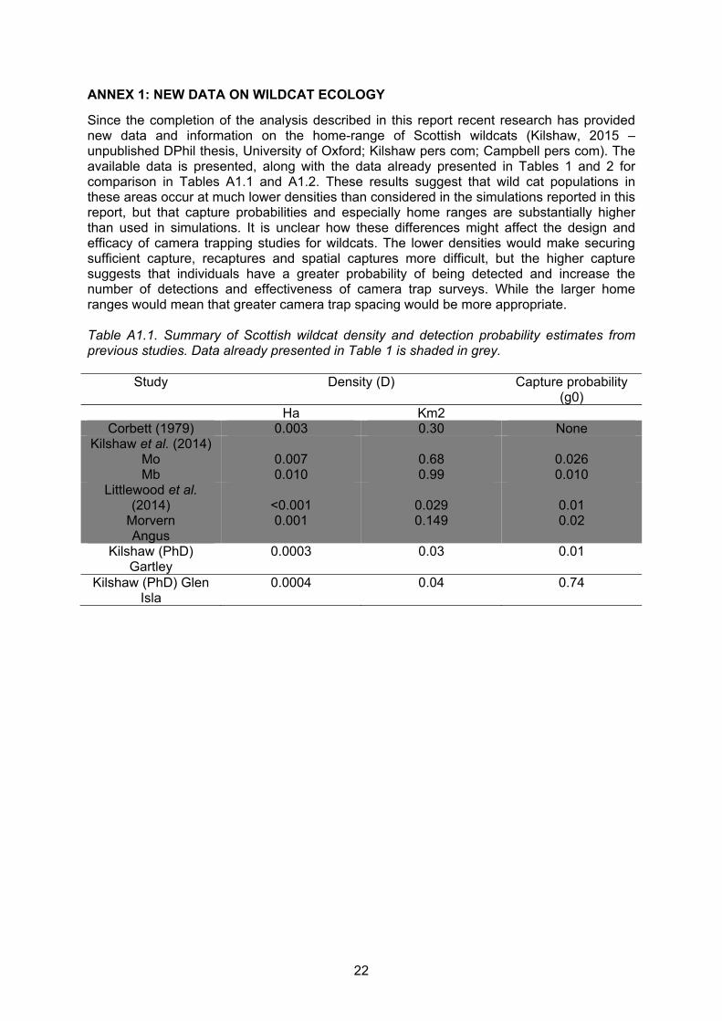
Since the completion of the analysis described in this report recent research has provided new data and information on the home-range of Scottish wildcats (Kilshaw, 2015 – unpublished DPhil thesis, University of Oxford; Kilshaw pers com; Campbell pers com). The available data is presented, along with the data already presented in Tables 1 and 2 for comparison in Tables A1.1 and A1.2. These results suggest that wild cat populations in these areas occur at much lower densities than considered in the simulations reported in this report, but that capture probabilities and especially home ranges are substantially higher than used in simulations. It is unclear how these differences might affect the design and efficacy of camera trapping studies for wildcats. The lower densities would make securing sufficient capture, recaptures and spatial captures more difficult, but the higher capture suggests that individuals have a greater probability of being detected and increase the number of detections and effectiveness of camera trap surveys. While the larger home ranges would mean that greater camera trap spacing would be more appropriate. Table A1.1. Summary of Scottish wildcat density and detection probability estimates from previous studies. Data already presented in Table 1 is shaded in grey.

Study Density (D) Capture probability (g0)

Ha Km2 Corbett (1979) 0.003 0.30 None

Kilshaw et al. (2014) Mo Mb

0.007 0.010

0.68 0.99

0.026 0.010

Littlewood et al. (2014)

Morvern Angus

<0.001 0.001

0.029 0.149

0.01 0.02

Kilshaw (PhD) Gartley

0.0003 0.03 0.01

Kilshaw (PhD) Glen Isla

0.0004 0.04 0.74

23

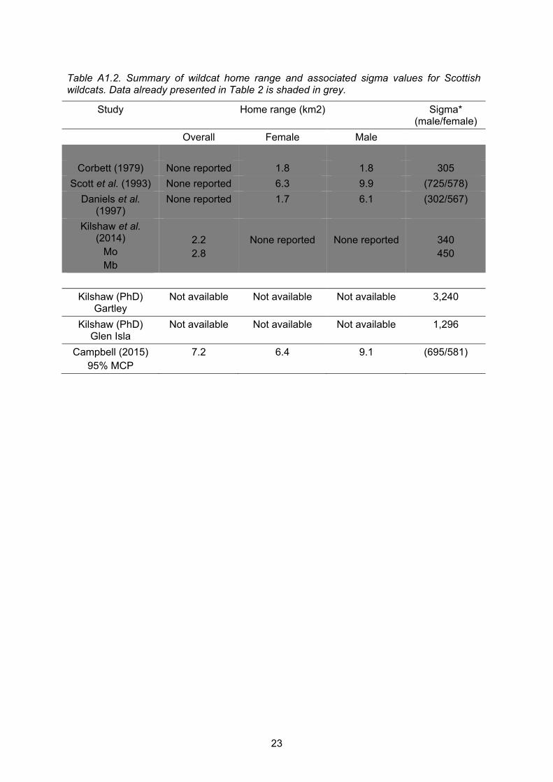
Table A1.2. Summary of wildcat home range and associated sigma values for Scottish wildcats. Data already presented in Table 2 is shaded in grey.

Study Home range (km2) Sigma* (male/female)

Overall Female Male

Corbett (1979) None reported 1.8 1.8 305

Scott et al. (1993) None reported 6.3 9.9 (725/578)

Daniels et al. (1997)

None reported 1.7 6.1 (302/567)

Kilshaw et al. (2014)

Mo Mb

2.2 2.8

None reported

None reported

340 450

Kilshaw (PhD) Gartley

Not available Not available Not available 3,240

Kilshaw (PhD) Glen Isla

Not available Not available Not available 1,296

Campbell (2015) 95% MCP

7.2 6.4 9.1 (695/581)

www.snh.gov.uk© Scottish Natural Heritage 2015 ISBN: 978-1-78391-359-6

Policy and Advice Directorate, Great Glen House,Leachkin Road, Inverness IV3 8NWT: 01463 725000

You can download a copy of this publication from the SNH website.