Scour in Cohesive Soils - Microsoft

Scour in Cohesive Soils

PUBLICATION NO. FHWA-HRT-15-033 MAY 2015

Research, Development, and TechnologyTurner-Fairbank Highway Research Center6300 Georgetown PikeMcLean, VA 22101-2296

FOREWORD

Scour in cohesive soils has been a challenge for engineers and designers. Unlike noncohesive soils, practical measurement techniques and well accepted guidance on the scourability of cohesive soils are severely lacking. This report summarizes a study through which an erosion testing device that simulates open channel flow on a small scale was developed and tested. In addition, a recommended design approach is provided that can be used for estimating scour for a range of cohesive soils. The study described in this report was conducted at the Federal Highway Administration Turner-Fairbank Highway Research Center J. Sterling Jones Hydraulics Laboratory.

Jorge E. Pagán-Ortiz Director, Office of Infrastructure Research and Development

Notice This document is disseminated under the sponsorship of the U.S. Department of Transportation in the interest of information exchange. The U.S. Government assumes no liability for the use of the information contained in this document. This report does not constitute a standard, specification, or regulation. The U.S. Government does not endorse products or manufacturers. Trademarks or manufacturers’ names appear in this report only because they are considered essential to the objective of the document.

Quality Assurance Statement The Federal Highway Administration (FHWA) provides high-quality information to serve Government, industry, and the public in a manner that promotes public understanding. Standards and policies are used to ensure and maximize the quality, objectivity, utility, and integrity of its information. FHWA periodically reviews quality issues and adjusts its programs and processes to ensure continuous quality improvement.

TECHNICAL REPORT DOCUMENTATION PAGE 1. Report No. FHWA-HRT-15-033

2. Government Accession No.

3. Recipient’s Catalog No.

4. Title and Subtitle Scour in Cohesive Soils

5. Report Date May 2015 6. Performing Organization Code

7. Author(s) Haoyin Shan, Jerry Shen, Roger Kilgore, and Kornel Kerenyi

8. Performing Organization Report No.

9. Performing Organization Name and Address GENEX SYSTEMS, LLC 2 Eaton Street, Suite 603 Hampton, VA 23669

10. Work Unit No. (TRAIS) 11. Contract or Grant No.

12. Sponsoring Agency Name and Address Office of Infrastructure Research and Development Federal Highway Administration 6300 Georgetown Pike McLean, VA 22101-2296

13. Type of Report and Period Covered Laboratory Report Feb. 2008–April 2014 14. Sponsoring Agency Code

15. Supplementary Notes The Contracting Officer’s Technical Representative (COTR) was Kornel Kerenyi (HRDI-50). 16. Abstract This study of scour in cohesive soils had two objectives. The first was to introduce and demonstrate a new ex situ erosion testing device (ESTD) that can mimic the near-bed flow of open channels to erode cohesive soils within a specified range of shear stresses. The ESTD employs a moving belt and a pump to generate a log-law velocity profile in a small test channel to simulate open channel flow. Successful testing requires careful preparation of soil specimens to avoid slaking. Preparation of erosion test samples by compaction usually leads to soil slaking, which cannot be tolerated to generate meaningful erosion function data. Therefore, cohesive soil specimens with different percentages of clay, silt, and non-uniform sands were mixed and de-aired in a pugger mixer to prevent slaking. The testing confirmed that the ESTD is capable of determining erosion characteristics of cohesive soils for bed shear stresses within the range of 0.063 to 0.31 lbf/ft2 (3 to 15 Pa). Its capability of directly measuring bed shear stresses enhances the understanding of the erosion process in cohesive soils. The second objective was to develop a method for estimating the critical shear stress and erosion rates for a limited range of cohesive soils in the context of the Hydraulic Engineering Circular 18 scour framework. The method is based on more easily obtained soil parameters so that direct erosion testing is not needed in all cases. General relations are proposed for both best-fit and design applications. Estimates of critical shear stress are based on the water content, fraction of fines, plasticity index (PI), and unconfined compressive strength. In addition, an equation for estimating erosion rates when bed shear stress exceeds critical shear stress is proposed. For application, the designer must determine the critical shear stress of the soil (from the previous relation), the unconfined compressive strength, and the PI. The guidance may be used for engineering design within limits based on the range of values in the current data set and to a lesser extent the range from Illinois field data on which parts of the methodology were validated. A Texas data set on which additional validation was attempted represents a distinct data set. The recommendations apply to fine grained cohesive soils within a range of plasticity and liquid limit (LL) characteristics. The PI should be within the range of 4 to 25 percent and the LL between 15 and 50 percent. The fraction of fines should fall between 10 and 90 percent. These methods best apply to soils with at least 90 percent saturation but can be used with lower degrees of saturation. 17. Key Words Cohesive soils, erosion testing, slaking, direct force gauge, log-law velocity profile, bed shear stress, critical shear stress, erosion rate

18. Distribution Statement No restrictions. This document is available to the public through the National Technical Information Service, Springfield, VA 22161. http://www.ntis.gov

19. Security Classif. (of this report) Unclassified

20. Security Classif. (of this page) Unclassified

21. No. of Pages 96

22. Price

Form DOT F 1700.7 (8-72) Reproduction of completed page authorized

SI* (MODERN METRIC) CONVERSION FACTORS APPROXIMATE CONVERSIONS TO SI UNITS

Symbol When You Know Multiply By To Find Symbol LENGTH

in inches 25.4 millimeters mm ft feet 0.305 meters m yd yards 0.914 meters m mi miles 1.61 kilometers km

AREA in2 square inches 645.2 square millimeters mm2

ft2 square feet 0.093 square meters m2

yd2 square yard 0.836 square meters m2

ac acres 0.405 hectares ha mi2 square miles 2.59 square kilometers km2

VOLUME fl oz fluid ounces 29.57 milliliters mL gal gallons 3.785 liters L ft3 cubic feet 0.028 cubic meters m3

yd3 cubic yards 0.765 cubic meters m3

NOTE: volumes greater than 1000 L shall be shown in m3

MASS oz ounces 28.35 grams glb pounds 0.454 kilograms kgT short tons (2000 lb) 0.907 megagrams (or "metric ton") Mg (or "t")

TEMPERATURE (exact degrees) oF Fahrenheit 5 (F-32)/9 Celsius oC

or (F-32)/1.8 ILLUMINATION

fc foot-candles 10.76 lux lx fl foot-Lamberts 3.426 candela/m2 cd/m2

FORCE and PRESSURE or STRESS lbf poundforce 4.45 newtons N lbf/in2 poundforce per square inch 6.89 kilopascals kPa

APPROXIMATE CONVERSIONS FROM SI UNITS Symbol When You Know Multiply By To Find Symbol

LENGTHmm millimeters 0.039 inches in m meters 3.28 feet ft m meters 1.09 yards yd km kilometers 0.621 miles mi

AREA mm2 square millimeters 0.0016 square inches in2

m2 square meters 10.764 square feet ft2

m2 square meters 1.195 square yards yd2

ha hectares 2.47 acres ac km2 square kilometers 0.386 square miles mi2

VOLUME mL milliliters 0.034 fluid ounces fl oz L liters 0.264 gallons gal m3 cubic meters 35.314 cubic feet ft3

m3 cubic meters 1.307 cubic yards yd3

MASS g grams 0.035 ounces ozkg kilograms 2.202 pounds lbMg (or "t") megagrams (or "metric ton") 1.103 short tons (2000 lb) T

TEMPERATURE (exact degrees) oC Celsius 1.8C+32 Fahrenheit oF

ILLUMINATION lx lux 0.0929 foot-candles fc cd/m2 candela/m2 0.2919 foot-Lamberts fl

FORCE and PRESSURE or STRESS N newtons 0.225 poundforce lbf kPa kilopascals 0.145 poundforce per square inch lbf/in2

*SI is the symbol for th International System of Units. Appropriate rounding should be made to comply with Section 4 of ASTM E380. e(Revised March 2003)

ii

TABLE OF CONTENTS

CHAPTER 1. INTRODUCTION .................................................................................................1 COHESIVE SOIL BEHAVIOR ...............................................................................................1 EROSION TESTING ................................................................................................................2 NEED ..........................................................................................................................................4

CHAPTER 2. LITERATURE.......................................................................................................7 CRITICAL SHEAR STRESS OF COHESIVE SOILS .........................................................7 EROSION RATES OF COHESIVE SOILS ...........................................................................8 EROSION TESTING DEVICES FOR COHESIVE SOILS .................................................9

CHAPTER 3. THE ESTD ...........................................................................................................11 THE MOVING BELT .............................................................................................................12 THE DIRECT FORCE GAGE ...............................................................................................13

Principle of Horizontal Measurement ....................................................................................13 Principle of Vertical Measurement ........................................................................................15

ADVANTAGES AND LIMITATIONS .................................................................................16

CHAPTER 4. MEASUREMENT OF FLOW AND BED SHEAR STRESS ..........................17 FLOW FIELD MEASUREMENT .........................................................................................17 SHEAR STRESS MEASUREMENT .....................................................................................23 FLOW/BED COMBINATIONS FOR EROSION TESTING .............................................27

CHAPTER 5. SOIL PREPARATION AND PROPERTIES ...................................................35 PREPARATION OF SOIL SPECIMENS .............................................................................35

Soil Preparation by Compaction ............................................................................................35 Soil Preparation with a Pugger Mixer ....................................................................................35 Soil Composition and Classification ......................................................................................36

ADDITIONAL GEOTECHNICAL PROPERTIES .............................................................39 Direct Shear Test ....................................................................................................................39 Unconfined Compression Test ...............................................................................................40

SLAKING .................................................................................................................................41 The Slaking Mechanism ........................................................................................................41 Slaking Test ...........................................................................................................................44

CHAPTER 6. EROSION TESTING PROTOCOL AND RESULTS .....................................47

CHAPTER 7. ANALYTICAL DEVELOPMENT ....................................................................55 EROSION RATE MODELS AND ESTIMATED PARAMETERS ...................................55

Power Model ..........................................................................................................................55 Linear Model ..........................................................................................................................57 Comparison and Selection .....................................................................................................58

CRITICAL SHEAR STRESS .................................................................................................59 United States Department of Agriculture (USDA) Model for Permissible Shear Stress.......61 Briaud Bounds .......................................................................................................................62 Power Model ..........................................................................................................................64

OTHER EROSION PARAMETERS.....................................................................................69 MODEL EVALUATION ........................................................................................................70 DESIGN EQUATIONS ...........................................................................................................72

iii

CHAPTER 8. CONCLUSIONS AND RECOMMENDATAIONS .........................................77

APPENDIX A. RELATION BETWEEN PI AND CLAY CONTENT ...................................81

REFERENCES .............................................................................................................................83

iv

LIST OF FIGURES

Figure 1. Graph. Generalized relationships for erosion in cohesive materials ................................2 Figure 2. Graph. Division of materials into zones for specific devices ...........................................3 Figure 3. Equation. Ultimate contraction scour ...............................................................................4 Figure 4. Equation. Time rate of contraction scour .........................................................................4 Figure 5. Equation. Ultimate pier scour ...........................................................................................5 Figure 6. Equation. Critical velocity and critical shear stress..........................................................5 Figure 7. Equation. Linear erosion law of cohesive soils ................................................................8 Figure 8. Equation. Exponential erosion law of cohesive soils .......................................................8 Figure 9. Equation. Wan and Fell equation for cohesive soil erosion .............................................9 Figure 10. Equation. Instantaneous shear stress equation for a jet ................................................10 Figure 11. Photo. The ESTD..........................................................................................................11 Figure 12. Diagram. Schematic of the ESTD ................................................................................12 Figure 13. Diagram. Dimensions of the moving belt.....................................................................13 Figure 14. Diagram. Principles of force measurements in the horizontal direction ......................14 Figure 15. Diagram. Principles of force measurements in the vertical direction ..........................15 Figure 16. Photo. The PIV system .................................................................................................18 Figure 17. Photo. The PIV illuminated laser .................................................................................18 Figure 18. Photo. The PIV measurement plane .............................................................................19 Figure 19. Graph. Velocity profiles of conduit flow with P220 sandpaper bed ............................20 Figure 20. Graph. Velocity profiles for belt-only tests with a P100 sandpaper bed ......................21 Figure 21. Graph. Combination velocity profiles at 0.58 gal/s (2.2 L/s) with a P80

sandpaper bed...........................................................................................................................22 Figure 22. Graph. Shear stress measurements of conduit flow on each sandpaper bed ................24 Figure 23. Equation. Bed-specific relation for conduit flow bed shear stress in the ESTD ..........24 Figure 24. Graph. Shear stress measurements of conduit flow......................................................25 Figure 25. Equation. Equation of bed shear stress for conduit flow in the ESTD .........................25 Figure 26. Graph. Shear stresses for combination tests on a P150 sandpaper bed ........................26 Figure 27. Equation. Dimensionless roughness height ..................................................................27 Figure 28. Equation. The law of the wall.......................................................................................28 Figure 29. Equation. Friction coefficient .......................................................................................28 Figure 30. Graph. Comparison of conduit flow point velocities on a P220 sandpaper bed ..........31 Figure 31. Graph. Conditions used for erosion testing in the ESTD .............................................32 Figure 32. Photo. The pugger mixer used for soil preparation ......................................................36 Figure 33. Graph. Particle-size distributions for Red Art clay, silt, and non-uniform sands ........37 Figure 34. Graph. Particle-size distributions of the cohesive soils tested in the ESTD ................38 Figure 35. Graph. Erosion curves of soils from a New Orleans levee...........................................43 Figure 36. Graph. Gradation of compacted clays ..........................................................................44 Figure 37. Photo. Slaking test on a compacted soil specimen .......................................................45 Figure 38. Graph. Slaking test results for soils 2 and 3 in still water ............................................46 Figure 39. Graph. Example data recorded for sample with soil index 4 .......................................48 Figure 40. Photo. Erosion soil sample 1W183 with increasing shear ...........................................49 Figure 41. Graph. Representative plots of erosion rate versus shear stress ...................................53 Figure 42. Equation. Power relationship between shear stress and erosion rate ...........................55 Figure 43. Graph. Measured and fitted power model for soil index 1 ...........................................57 Figure 44. Equation. Linear relationship between shear stress and erosion rate ...........................58

v

Figure 45. Graph. Estimated critical shear stress comparison .......................................................59 Figure 46. Graph. Comparison of FHWA, Illinois, and Texas soil data .......................................60 Figure 47. Equation. USDA equation for permissible shear stress ................................................62 Figure 48. Graph. Comparison of permissible and critical shear stress.........................................63 Figure 49. Equation. Briaud equation for critical shear stress lower bound ..................................63 Figure 50. Equation. Briaud equation for critical shear stress upper bound ..................................63 Figure 51. Graph. Comparison of critical shear stress with Briaud bounds ..................................64 Figure 52. Equation. General power model ...................................................................................64 Figure 53. Graph. Critical shear versus unconfined compressive strength ....................................66 Figure 54. Equation. Predictive relation for critical shear stress ...................................................66 Figure 55. Graph. Comparison of predicted versus estimated critical shear stress .......................67 Figure 56. Equation. Water content at 100-percent saturation ......................................................67 Figure 57. Graph. Critical shear stress comparison with FHWA, Illinois, and Texas data ...........68 Figure 58. Equation. Predictive relation for C1 ..............................................................................69 Figure 59. Graph. Predictive relation for the multiplier coefficient ..............................................70 Figure 60. Equation. Erosion rate model .......................................................................................70 Figure 61. Graph. Predicted versus measured erosion rates ..........................................................71 Figure 62. Graph. Predicted versus measured erosion rates with Illinois data ..............................72 Figure 63. Equation. Design equation for critical shear stress ......................................................72 Figure 64. Graph. Design equation for critical shear stress compared with data ..........................74 Figure 65. Equation. Design equation for C1 .................................................................................74 Figure 66. Graph. Design equation for erosion rate compared with data ......................................75 Figure 67. Graph. Relationship between PI and clay percentage ..................................................81 Figure 68. Equation. Linear relationship between PI and clay percentage ....................................81

vi

LIST OF TABLES

Table 1. Bed materials ...................................................................................................................19 Table 2. Time interval validation tests ...........................................................................................23 Table 3. ESTD shear stress parameters for rectangular conduit tests ............................................24 Table 4. Consecutive day validation shear tests ............................................................................27 Table 5. Relationship between f, r, ks, and ks

+ ...............................................................................29 Table 6. Particle size and modeled roughness height ....................................................................29 Table 7. Equations for the constant B ............................................................................................30 Table 8. Test conditions for the ESTD ..........................................................................................33 Table 9. Classification and composition of soils for testing ..........................................................37 Table 10. Mass and moisture properties of soils prepared by pugger mixer .................................39 Table 11. Mass and moisture properties of soils prepared by compaction ....................................39 Table 12. Additional geotechnical properties of soils prepared by pugger mixer .........................40 Table 13. Additional geotechnical properties of soils prepared by compaction ............................40 Table 14. Properties of four soils from a New Orleans levee ........................................................42 Table 15. Erosion test matrix and results for soils prepared by pugger mixer ..............................50 Table 16. Estimated critical shear stress parameters for the power model ....................................56 Table 17. Estimated critical shear stress parameters for the linear model .....................................58 Table 18. Data set parameter summary ..........................................................................................61

vii

LIST OF ACRONYMS

ASSET Adjustable shear stress erosion and transport flume CCFED Circular Couette flow erosion device EFA Erosion function apparatus ESTD Ex situ scour test device HEC-18 Hydraulic Engineering Circular 18 HET Hole erosion test JET Jet erosion test LL Liquid limit PI Plasticity index PL Plastic limit PIV Particle image velocimetry Re Reynolds number SEDflume Sediment erosion at depth flume SERF Sediment erosion rate flume USCS Unified Soil Classification System USDA United States Department of Agriculture

viii

LIST OF SYMBOLS

α Pier diameter (or width), ft (m) c Cohesion, lbf/ft2 (N/m2 or Pa) D50 Median grain size, inches (mm) e Void ratio, dimensionless F Fraction of soil passing #200 sieve (0.075 mm) g Acceleration due to gravity, 32.2 ft/s2 (9.81 m/s2) h Nozzle height above the soil surface, ft (m) Jp Potential jet core length, ft (m) Ji Instantaneous jet orifice height, ft (m) k Slope of the erosion curve, dimensionless K1 Correction factor for pier nose shape, dimensionless K2 Correction factor for angle of attack of flow, dimensionless kf Empirical floc erosion rate, lb/ft2/s (g/m2/s) kL Empirical erosion constant, lb/ft2/s (g/m2/s) ks Roughness height, inches (µm) n Manning’s roughness coefficient, dimensionless Q Flow rate in the ESTD test channel, gal/s (L/s) qu Unconfined compression strength, lbf/ft2 (N/m2 or Pa) S Degree of saturation, dimensionless Sg Sediment specific gravity, dimensionless t Duration of flow or test, h u Velocity at a depth y, ft/s (m/s) u* Shear velocity, ft/s (m/s) umax Maximum flow velocity at the boundary layer thickness, ft/s (m/s) V1 Mean velocity of flow directly upstream of the pier, ft/s (m/s) V2 Average flow velocity in the contracted section, ft/s (m/s) Vc Critical velocity, ft/s (m/s) w Water content, dimensionless y1 Upstream average flow depth, ft (m) ys,u Ultimate scour depth, ft (m) ys(t) Scour depth at time, t, ft (m)

ix

z Depth from soil surface, inches (mm)

ż Erosion rate, inches/h (mm/h) ż i Initial rate of scour, ft/h (m/h) ż M Mass erosion rate, lb/ft2/s (g/m2/s)

α Unit conversion constant, value and dimensions are equation-specific δ Boundary layer thickness, ft (m)

Von Karman constant ν Kinematic viscosity of water, ft2/s (m2/s) ρ Density, lb/ft3 (kg/m3) τ Hydraulic shear stress, lbf/ft2 (N/m2 or Pa) τ c Critical shear stress for the initiation of erosion, lbf/ft2 (N/m2 or Pa) τ c(z) Critical shear stress at a depth of z, lbf/ft2 (Pa) τ i Instantaneous peak boundary shear stress, lbf/ft2 (N/m2 or Pa) τ p Soil permissible shear stress, lbf/ft2 (Pa) φ Friction angle, degree (radian)

κ

x

CHAPTER 1. INTRODUCTION

Cohesive soils generally include fine-grained silt and clay mineral particles passing the No. 200 sieve (less than 0.003 inches (0.075 mm)). These particles usually have a shape of small flat plates, needles, or tubes with a high specific area defined as the ratio of surface area to volume.(1) In the presence of water, these particles are subjected to physicochemical forces that are large in comparison with their weight, which tends to hold the soil mass together. These physicochemical forces are more dominant than the submerged particle weight in resisting erosion (scour). However, attempting to apply an understanding of the physicochemical forces on the micro level is challenging and may not yield practical results because erosion of cohesive soils generally occurs at the more macro scale of clumps of soil rather than individual particles.

COHESIVE SOIL BEHAVIOR

Many parameters influence the erosion of cohesive soils. These parameters include the physical and chemical properties of soil, as well as the physical, chemical, and mechanical characteristics of the eroding fluid.

The physical and chemical properties of soil include the following:

• Soil temperature. • Dominant ions of the clay. • Sodium adsorption ratio. • Cation exchange capacity. • Type of clay mineral. • Clay content. • Organic matter content. • Swelling. • Plasticity index (PI). • Particle size distribution of the noncohesive fraction. • Water content. • Void ratio. • Consolidation. • Stratification.

The following physical, chemical, and mechanical characteristics of the eroding fluid may contribute to erosion:

• Soil pore fluid pH. • Soil pore fluid salinity. • Fluid temperature. • Hydrodynamic forces of the moving fluid at the soil/fluid boundary (shear stress).

The scope of this study does not include consideration of the erosion effects of the physical or chemical characteristics of the eroding fluid and assumes that they are constant for the laboratory testing of erosion.

1

Another soil loss process that may occur when a soil is not saturated and then exposed to flowing water is slaking. This mechanism will be discussed separately from the soil erosion process because it is a distinctly different process that can accelerate erosion.

Hydraulic Engineering Circular 18 (HEC-18) provides a conceptual framework (shown here in figure 1) relating shear stress, soil types, and erosion rates for a variety of materials, including cohesive soils.(2) Erodibility is divided into six categories for materials ranging from very highly erodible fine sands and non-plastic silts to non-erosive rock. However, this broad categorization is not directly useful for site-specific erosion or scour computations because of the wide range in types of soils and the wide range of erosion rates for a given type of soil. (The two-letter soil type codes are from the Unified Soil Classification System (USCS) that is discussed later.)

1 inch = 25.4 mm. 1 lbf/ft2 = 47.8 Pa.

Figure 1. Graph. Generalized relationships for erosion in cohesive materials.

EROSION TESTING

One of the few strategies available today for the design engineer to determine site-specific soil erosion rates is to conduct erosion tests on the specific soil. Because the appropriate range of shear stresses needed for a range of soil types may vary by orders of magnitude, a single device is unlikely to be able to adequately test all materials. Figure 2 illustrates a division of the shear stress axis into five shear stress ranges and suggests the types of materials that could be tested using a device capable of delivering those shear stresses. This report describes a device targeted to the second (highlighted) of the five shear stress ranges, which should be capable of measuring erosion rates for many soils classified as ML (inorganic silts, very fine sands, rock flour, silty or

2

clayey fine sands) and CL (inorganic clays of low to medium plasticity, gravelly clays, sandy clays, silty clays, lean clays).

1 inch = 25.4 mm. 1 lbf/ft2 = 47.8 Pa.

Figure 2. Graph. Division of materials into zones for specific devices.

Experimental modeling remains an indispensable method for understanding the erosion mechanism. In addition to flume modeling, several small-scale devices have been developed for the specific purpose of testing soil/rock erodibility. However, these devices may simulate flow conditions that do not mimic the conditions experienced with open channel flow, particularly the velocity distribution. Because different flow conditions will generate distinct dynamic forces on the tested cohesive soils, the type of testing apparatus and bed size may influence the test results. In some cases, such testing may result in designs for scour prediction that are not protective of the traveling public.

Therefore, a device that can simulate the open channel flow profile approximated by the log-law velocity profile is urgently needed. If a testing device reproduces the log-law velocity profile, then it will be capable of generating hydrodynamic forces on the bed similar to those in an open channel and, therefore, better mimicking the erosion process.

Development of sensors that can accurately and reliably measure the forces acting on the bed is another key challenge in developing a small-scale erosion testing device. Direct force measurements with a servo-controlled mechanism are available to instantaneously measure hydrodynamic forces on soil specimens and can be incorporated into erosion testing devices.

0.1

1

10

100

1000

10000

100000

0.1 1 10 100 1000 10000 100000Shear stress (Pa)

Very high Erodibility

I

HighErodibility

II

MeduimErodibility

IIILow

ErodibilityIV

Very Low Erodibility

V

Non-erosiveVI

SPSM

MLML

CL CHRock

CL

CH

Eros

ion

Rate

(mm

/h)

3

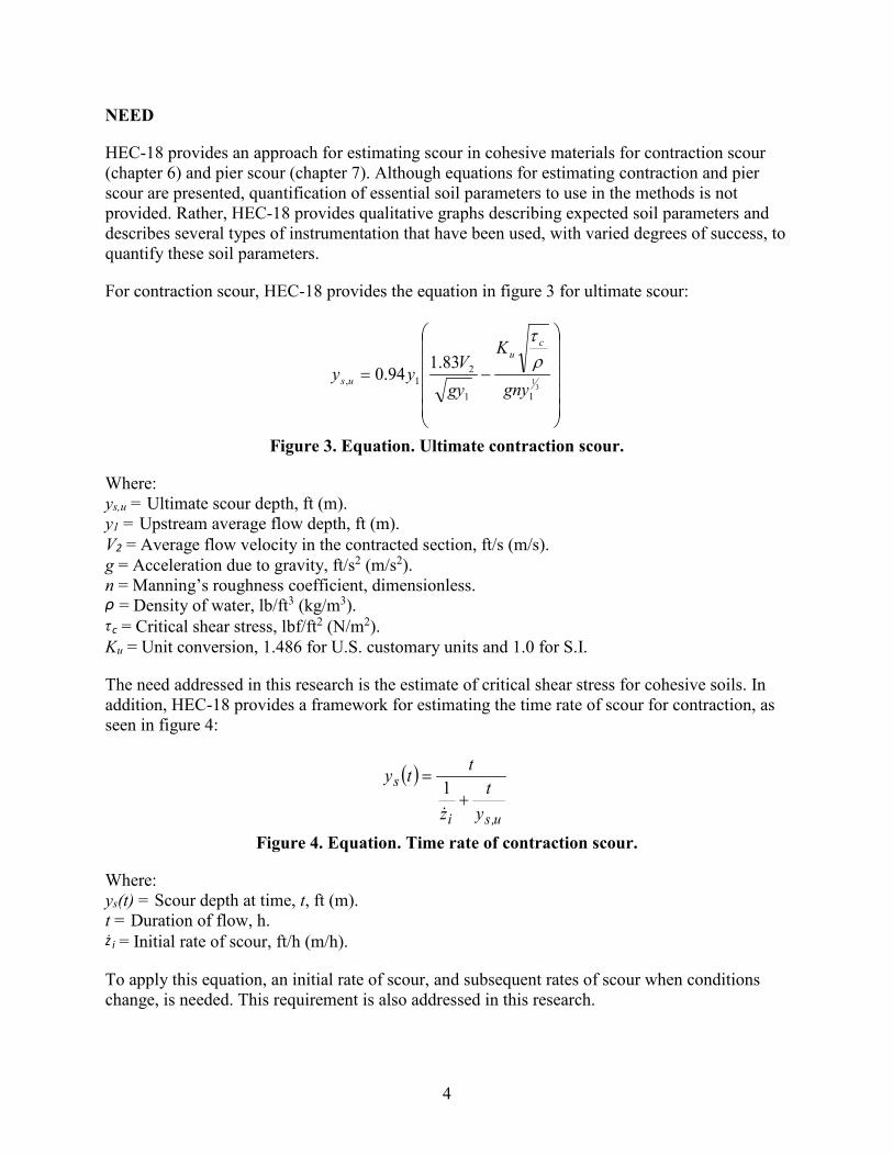
NEED

HEC-18 provides an approach for estimating scour in cohesive materials for contraction scour (chapter 6) and pier scour (chapter 7). Although equations for estimating contraction and pier scour are presented, quantification of essential soil parameters to use in the methods is not provided. Rather, HEC-18 provides qualitative graphs describing expected soil parameters and describes several types of instrumentation that have been used, with varied degrees of success, to quantify these soil parameters.

For contraction scour, HEC-18 provides the equation in figure 3 for ultimate scour:

Figure 3. Equation. Ultimate contraction scour.

Where: ys,u = Ultimate scour depth, ft (m). y1 = Upstream average flow depth, ft (m). V2 = Average flow velocity in the contracted section, ft/s (m/s). g = Acceleration due to gravity, ft/s2 (m/s2). n = Manning’s roughness coefficient, dimensionless.

= Density of water, lb/ft3 (kg/m3). c = Critical shear stress, lbf/ft2 (N/m2).

Ku = Unit conversion, 1.486 for U.S. customary units and 1.0 for S.I.

The need addressed in this research is the estimate of critical shear stress for cohesive soils. In addition, HEC-18 provides a framework for estimating the time rate of scour for contraction, as seen in figure 4:

Figure 4. Equation. Time rate of contraction scour.

Where: ys(t) = Scour depth at time, t, ft (m). t = Duration of flow, h.

i = Initial rate of scour, ft/h (m/h).

To apply this equation, an initial rate of scour, and subsequent rates of scour when conditions change, is needed. This requirement is also addressed in this research.

−=3

1

11

21,

83.194.0gny

K

gyVyy

cu

usρτ

ρ τ

( )

u,si

s

yt

z

tty+

=

1

ż

4

For ultimate pier scour, HEC 18 provides the equation in figure 5:

Figure 5. Equation. Ultimate pier scour.

Where: K1 = Correction factor for pier nose shape, dimensionless. K2 = Correction factor for angle of attack of flow, dimensionless. a = Pier diameter (or width), ft (m). V1 = Mean velocity of flow directly upstream of the pier, ft/s (m/s). Vc = Critical velocity for initiation of erosion of the cohesive material, ft/s (m/s).

Determination of the critical velocity for a soil is needed to apply this equation. Critical velocity is related to critical shear stress and the hydraulic parameters of the stream as shown in figure 6. Therefore, no additional soil information is required for computation of pier scour beyond that required for contraction scour. Time rate of pier scour is computed in the same manner described for time rate of contraction scour.

Figure 6. Equation. Critical velocity and critical shear stress.

Where: y1 = Depth of water approaching the pier, ft (m).

Therefore, the need addressed by this research is to provide quantitative tools for determining critical shear stress, c, and erosion rate, , for cohesive soils. The critical shear stress is essential for determining an ultimate scour depth and, in many situations, may be all that is required. For situations where a more detailed assessment is needed, the erosion rate may be used for a time-dependent scour assessment.

This study has two objectives. The first objective is to introduce and demonstrate the effectiveness of a new ex situ erosion testing device that can mimic the near-bed flow of open channels to erode cohesive soils within a specified range of shear stresses. The new ex situ scour test device (ESTD) uses a moving belt and a pump to generate a log-law velocity profile in a channel. The ESTD is designed to maintain a constant bed shear stress throughout the test period. Cohesive soil samples mixed with Red Art clay (Illite), silt, and sands were created in the laboratory and tested in the ESTD to demonstrate the operations and effectiveness of the device.

The second objective is to develop a method for estimating the key erosion parameters of a limited range of cohesive soils based on more easily obtained soil parameters so that direct erosion testing is not needed in all cases. General relations are proposed in this report.

701650

2162

22.

c.u,s g

VV.aKK.y

−=

6

11

cuc y

gnK

V

ρτ

=

τ ż

5

Chapter 2 features a brief literature review of erosion processes in cohesive soils. Chapter 3 describes the design and operation of the ESTD. Chapter 4 describes how the log-law velocity profile is reproduced in the test channel and how boundary shear stress is measured with the device. Chapter 5 details the preparation of soil specimens and the soil sample properties. Chapter 6 describes erosion tests and results. Chapter 7 discusses the factors affecting erosion and summarizes the analytical development of the recommended design relations. Chapter 8 includes conclusions and future research recommendations.

6

CHAPTER 2. LITERATURE

The literature relevant to this research was reviewed and divided into three main categories: critical shear stress, erosion rates, and erosion testing devices. Design guidance has typically related to critical velocity, critical shear stress, and/or erosion rate. Critical velocity is defined as the velocity at which soil erosion is initiated. Similarly, critical shear stress is the shear stress at which the soil erosion is initiated. For cohesive soils, the ability to determine these values, and the erosion rates once they are exceeded, has been largely accomplished by various erosion testing devices.

CRITICAL SHEAR STRESS OF COHESIVE SOILS

Before 1955, critical velocity was used to determine whether cohesive soils would erode. During the 1950s, researchers moved to the critical shear stress of soils as a more direct indication of the erodibility of a particular soil because critical velocity depended on other hydraulic parameters.

A critical shear stress may be assigned to a specific cohesive soil. It was assumed that if the eroding shear stress exceeds the critical shear stress, then a soil will experience erosion. In this framework, critical shear stress is considered a soil property. Researchers attempted to correlate it to other soil properties as a means of predicting its value for a given soil. Dunn correlated the critical shear stress to soil vane shear strength, PI, and clay fraction (particles less than 0.0024 inches (0.060 mm)).(3) Smerdon and Beasley related critical shear stress to the PI, dispersion ratio, mean particle size of clay, and percentage of clay.(4,5) Several investigators proposed using a power law of bulk density to reflect the critical shear stress of a soil.(6,7)

Straub and Over found a linear relationship between soil critical shear stress and the logarithm of the unconfined compressive strength in undisturbed cohesive soils in Illinois.(8) In that work, the critical shear stresses of undisturbed field soils were extrapolated from erosion testing using the erosion function apparatus (EFA).

However, other researchers have stated that erosion in cohesive soils is essentially a surface phenomenon and should not be related to a bulk engineering properties such as unconfined compressive strength.(9) Previous studies have explored relations between erosion characteristics and properties such as vane shear strength, unconfined compressive strength, and dry unit weight but have not found useful relations. (See references 10 through 13.)

Some researchers argued that the critical shear stress definition is arbitrary because different observers would interpret different thresholds for critical shear stress. In addition, it was thought that the critical shear stress would also be affected by the flow condition. For example, identical soils experiencing open channel flow versus periodic flow like ocean waves would have different critical shear stresses.

In addition to these challenges, determining the critical shear stress for a particular soil does not equip a design engineer with information about erosion rates once the critical shear stress is exceeded. Knowing the critical shear stress also does not provide information on the spatial extent of erosion. Erosion rates and erosion spatial properties also vary based on the flow conditions.

7

EROSION RATES OF COHESIVE SOILS

The erosion rate is defined by both the flow condition and the soil properties. Most research concerning erosion rates to date has focused on surficial marine sediments or soft muds that have a wet bulk density between 31 to 81 lb/ft3 (500 to 1,300 kg/m3).(14,15) In some of these conditions, the water content (the ratio of water mass to soil mass) is equal to or larger than 100 percent. Depending on the apparatus and test methods used, only a limited depth of surficial mud might be tested. The wet bulk density of bottom mud can increase to 110 lb/ft3 (1,800 kg/m3) because of consolidation.

For these kinds of soils, researchers proposed two erosion formulations: linear law and exponential law. The linear law is written in the form seen in figure 7.(16)

Figure 7. Equation. Linear erosion law of cohesive soils.

Where: żM = Mass erosion rate, lb/ft2/s (g/m2/s). kL = Empirical erosion constant, lb/ft2/s (g/m2/s). τ = Hydraulic shear stress, lbf/ft2 (Pa). τc(z) = Critical shear stress at a depth of z, lbf/ft2 (Pa). z = Depth from soil surface, inches (mm).

The exponential law has the form seen in figure 8:

Figure 8. Equation. Exponential erosion law of cohesive soils.

Where: kf = Empirical floc erosion rate, lb/ft2/s (g/m2/s).

, = Empirical constants.

Mehta and Partheniades divided erosion test results into Type I and II based on the erosion profile and the change in shear stress applied to the soil.(17) In both cases, an erosion profile with increasing shear resistance with soil depth is assumed. The difference between the two types of erosion is defined by the relative time scale of the shear stress applied to the soil compared with the depletion (or erosion) time scale of the soil. Type I behavior is observed when the time scale of the shear stress is long compared with the time scale of the soil depletion. This case is referred to as depth limited erosion, in which an exponential decay in the erosion rate is experienced. The equation in figure 8 is used for this type. Type II behavior is observed when the time scale of the shear stress is short compared with the time scale of the soil depletion. This case is referred to as unlimited erosion, in which a linear increase in the erosion rate is experienced. The equation in figure 7 is used for this type.(18)

�̇�𝑧𝑀𝑀 = 𝑘𝑘𝐿𝐿𝜏𝜏 − 𝜏𝜏𝑐𝑐(𝑧𝑧)𝜏𝜏𝑐𝑐(𝑧𝑧)

�̇�𝑧𝑀𝑀 = 𝑘𝑘𝑓𝑓𝑒𝑒𝑒𝑒𝑒𝑒 �𝛼𝛼�𝜏𝜏 − 𝜏𝜏𝑐𝑐(𝑧𝑧)�𝛽𝛽�

α β

8

EROSION TESTING DEVICES FOR COHESIVE SOILS

Researchers have developed several devices to study scour in cohesive soils by measuring the forces involved in the scour process. Moore and Masch developed a circular Couette flow erosion device (CCFED).(19) The device provides a stationary mount attached to a torsion wire for a circular soil specimen. An outer drum, concentric with the soil specimen, contains the eroding fluid between it and the soil specimen. The outer drum is rotated by a variable speed motor, and a shear stress is consequently transmitted to the soil specimen surface, which can be directly measured by knowing the angular displacement of the torsion wire. The erosion rate of cohesive sediments is determined from the loss of mass within the testing time interval.

Other apparatus have been proposed to estimate critical shear stress in cohesive soils. These devices include the following:

• Sediment erosion at depth flume (SEDflume).(20) • Jet erosion test (JET).(21) • Erosion function apparatus (EFA).(22) • Adjustable shear stress erosion and transport flume (ASSET).(23) • Hole erosion test (HET).(24) • Sediment erosion rate flume (SERF).(25)

Trammell detailed the motivation, testing procedures, data analysis, advantages, and limitations of the ASSET, EFA, SEDflume, and SERF devices.(26) The following discussion focuses on the description of HET and JET to provide a range of the types of devices available.

For the HET, a clay specimen is inserted into a confining tube connecting two water tanks with different water levels. A pinhole is bored in the center of the specimen. Water flows through the pinhole, exerting shear stress to erode the specimen. The flow velocity is increased steadily until entrainment occurs. At the end of each time increment, the eroded outflow is collected to obtain the erosion rate, and the average diameter of the enlarged hole is calculated. The shear stress is estimated from the head loss between the two tanks. For this computation, the friction coefficient can be obtained from the Moody chart. An erosion curve (erosion rate versus shear stress) is plotted and then fit to the equation seen in figure 9.(24)

Figure 9. Equation. Wan and Fell equation for cohesive soil erosion.

Where: M = Mass erosion rate, lb/ft2/s (g/m2/s).

k = Slope of the erosion curve, dimensionless. = Hydraulic shear stress along the hole, lbf/ft2 (Pa). c = Critical shear stress for the initiation of erosion, lbf/ft2 (Pa).

For the JET, sediment is placed in the bottom of an open tank. An adjustable constant-head tank supplies water to a vertical tube submerged in the open tank, creating an impinging jet of water on the sediment. By converting potential energy to kinetic energy, the jet obtains a certain

�̇�𝑧𝑀𝑀 = 𝑘𝑘(𝜏𝜏 − 𝜏𝜏𝑐𝑐)

ż

τ τ

9

velocity to erode the sediments. The jet nozzle typically has a diameter of 0.25 inches (6.4 mm). The nozzle height above the soil surface can be adjusted in a range of 1.6 to 8.7 inches (40 to 220 mm). After the test time period, a point gage with the equivalent diameter of the nozzle is inserted in the tube to shut off the jet and measure the erosion depth. The instantaneous shear stress is calculated using the equation in figure 10.(27)

Figure 10. Equation. Instantaneous shear stress equation for a jet.

Where: i = Instantaneous peak boundary shear stress, lbf/ft2 (Pa). = Fluid density, lb/ft3, (kg/m3).

g = Acceleration due to gravity, 32.2 ft/s2 (9.81 m/s2). h = Nozzle height above the soil surface, ft (m). JP = Potential jet core length (taken as 6.3 times the jet nozzle diameter), ft (m). Ji = Instantaneous jet orifice height, ft (m).

The critical shear stress is determined by plotting the measured values of Ji and i. Because the equilibrium scour depth is not reached within the test period, it is extrapolated from the measured data. The shear stress is then calculated for that depth from the equation in figure 10. From these data, the critical shear stress can be calculated.

Although each device measures soil erosion in some manner, they differ regarding the types of erosion that is being measured in the following ways:

• The ASSET flume and SEDflume simulate open channel flow erosion. • The EFA and SERF simulate conduit flow erosion. • The HET simulates the seepage process. • The JET simulates erosion under a jet. • The CCFED simulates a shallow circular Couette flow erosion process.

Different flow conditions generate distinct dynamic forces on tested cohesive soils. For bridge safety design, a device that can simulate the log-law flow condition in open channels is urgently needed. The reproduced log-law flow condition generates similar hydrodynamic forces, meaning that the erosion process in open channels can be reproduced.

𝜏𝜏𝑖𝑖 = 0.00416𝜌𝜌(2𝑔𝑔ℎ) �𝐽𝐽𝑒𝑒𝐽𝐽𝑖𝑖�

2

τ ρ

τ

10

CHAPTER 3. THE ESTD

Because many erosion measurement devices do not duplicate open channel flow conditions or are too large and bulky for cost-effective routine testing, the ESTD was developed. It uses a moving belt and centrifugal pump to generate a log-law velocity profile in a channel where the tested soil is flush with the channel bottom.

The ESTD is designed to measure the erodibility of a cylindrical soil specimen under well-controlled flow conditions. The soil specimen has a diameter of 2.5 inches (63.5 mm) and a height of 0.6 inches (15 mm). The system has a total volume of about 145 gal (550 L). The device includes three tanks: an inlet tank, an ESTD tank, and an outlet tank. Inlet and outlet tanks are connected with a rectangular channel located in the ESTD tank. The channel is 22.8 inches (580 mm) long, 4.7 inches (120 mm) wide, and 0.79 inches (20 mm) deep. The device includes a flow meter and a direct force gauge to measure the force imparted by the flowing water on the soil sample. Figure 11 shows a three-dimensional representation of the ESTD.

Figure 11. Photo. The ESTD.

Two cascaded filter cylinders (Shelco, model: 12FOS3) filter the fluid in the system. Each cylinder has a diameter of 1.4 ft (0.42 m) and a height of 4.1 ft (1.25 m), housing twelve 2.5-ft (0.75-m)-tall wound filter cartridges with a filtration capacity of 0.00002 inches (0.0005 mm). The filtration ensures that the fluid near soil specimens is always clear for observation.

11

Water is propelled by a moving belt above the test channel and a pump as shown in figure 12. A moving belt rolls above the channel in the ESTD tank. The flow velocity profile is S-shaped when only the moving belt is propelling water.(28) The velocity profile takes the form of a parabola in the rectangular test channel when the belt is not moving as illustrated at section (1) in figure 12. Combining the S-shape profile from the belt alone with the parabolic profile from the pump alone may result in the desired log-law velocity profile as illustrated in figure 12 at section (2).

A range of grades of sandpaper are attached to the bottom of the channel to simulate bed roughness. The sandpaper grades are described later in this report.

Figure 12. Diagram. Schematic of the ESTD.

THE MOVING BELT

The moving belt has dimensions shown in figure 13. The roughness elements on the belt are 0.197 inches (5 mm) wide and 0.201 inches (5.1 mm) high. The net spacing between two adjacent roughness elements is 1.53 inches (38.8 mm). The distance from the roughness elements bottom to the ESTD tank bottom is 0.73 inches (18.5 mm).

The moving belt is enclosed in an aluminum case to minimize the influence of belt vibration on the flow beneath the belt. The case has a cutout on the bottom to expose the belt to the water in the channel. The width of the cutout is 4.53 inches (115 mm). Gaps exist between the belt and the two cutout boundaries. Total width of these two gaps is 0.59 inches (15 mm). The belt and aluminum case are mounted on the lid of the ESTD tank. This lid is closed during testing.

12

1 inch = 25.4 mm.

Figure 13. Diagram. Dimensions of the moving belt.

THE DIRECT FORCE GAGE

The ESTD is capable of instantaneously and precisely measuring horizontal shear and vertical forces on a soil specimen with a direct force gauge. The direct force gauge is specifically designed to measure small forces in a wet environment. A rubber membrane separates it into wet and dry parts. The core is a platform held by a bronze leaf spring. On top of the platform sits the sensor disk whose deflection indicates the magnitude of the shear force. A test soil specimen is fixed to the sensor disk so that the eroding forces acting on a soil specimen from the flow are directly measured.

Underneath the platform, a carrier holds two horizontally mounted permanent magnets that dip into two solenoids: SERVO and CALIBRATION. The magnet movement generates a counter movement to the sensor disk that keeps it in a fixed position with residual deflection of 0.0027 inches (0.068 mm) at 2.1 lb/ft2 (100 Pa). The principles of force measurements in the horizontal and vertical directions are applied as follows.

Principle of Horizontal Measurement

Assume a fluid-induced force, Fw, pushed the platform to right as shown in figure 14. A small horizontal deflection of the sensor disk will occur. This deflection moves the center magnet to the right and generates a positive error-voltage at the HALL Sensor. This voltage is amplified and drives a current through the SERVO-Solenoid. This current generates a magnetic field and pushes the permanent magnet to the left with a magnetic force, Fm. This motion lasts until the error-voltage at the HALL sensor diminishes to zero. A residual deflection of the platform always exists to generate the corresponding counterforce to the shear force.

13

Figure 14. Diagram. Principles of force measurements in the horizontal direction.

The current through the SERVO-Solenoid is proportional to the induced force Fw. The correlation between the solenoid current and the generated magnetic force Fm is highly linear. This correlation indicates that the measurement of current represents the measurement of Fw. As all parameters in this SERVO loop are constant, the current measured with high accuracy is a basis for subsequent signal processing to obtain the shear force.

The accuracy and stability of this type of sensor is enhanced because the platform has virtually no deflection, which offers the following advantages:

1. The sensor disk does not dive (change elevation) because of vertical deflection.

2. Mutation of the leaf springs due to corrosion or plaque does not materially affect the accuracy because they simply hold the platform.

3. A small gap between the sensor disk and the aperture ring is obtainable.

With respect to the gap between the sensor disk and aperture ring, it is conceivable that eroded clay particles in the fluid could be captured at the gap hindering accurate measurement. Therefore, a gap of 0.039 inches (1.0 mm) is preferred.

14

A built-in calibrator provides a valuable tool to calibrate the device. It utilizes the same principle discussed. For calibration, the induced force and the counterforce Fc are reversed compared with their use during testing.

Principle of Vertical Measurement

The deflection of the horizontally fastened bronze plate spring shown in figure 15 indicates that a vertical force is induced. The front view shows how the spring is mounted on the platform. On the bottom of the plate spring, a magnet is fixed to the end of a magnet holder. The gap between the sensor and the magnet is about 0.039 inches (1.0 mm).

Figure 15. Diagram. Principles of force measurements in the vertical direction.

When a vertical force, dF, is induced to the sensor disk, the bronze plate spring bends with a small deflection, dz. The magnet is also lowered the same dz, which results in the change of magnetic field of the permanent magnet. The HALL sensor converts this change into a voltage signal, dU. The relations between the force, dF, the deflection, dz, and the voltage, dU, are highly linear. As with the horizontal measurement, this linearity allows precise determination of the vertical force. The measurement range of vertical force is 0 to 0.225 lbf (0 to 1 N) corresponding to 0 to 0.225 lb (0 to 102 g) of soil.

15

ADVANTAGES AND LIMITATIONS

An important advantage of the ESTD is that the horizontal and vertical measurements work independently. Any vertical force slightly lowers the magnets Z1 and Z2 a maximum of 0.0039 inches (0.10 mm). However, this change does not influence the horizontal deflection of the platform or the shear stress. Similarly, any horizontal force will slightly push the platform horizontally a maximum of 0.0027 inches (0.068 mm), but this change does not affect the vertical magnetic fields. This independence allows simultaneous and precise measurements of both the horizontal and vertical forces.

One challenge for this type of force gauge is that it requires the test surface to be flush with the surrounding fixed surface when used in air.(29) Any depression or protrusion can result in additional forces resulting from flow disturbances caused by these surface discontinuities. For the ESTD, these forces essentially affect the initial shear stress measurement when defining the entrainment of clay clumps. Once erosion starts, the gauge measures the actual shear force on the soil specimen as in the field conditions when its shape evolves.

At the beginning of the test, a soil specimen is placed flush with the channel bottom. As erosion occurs, the specimen is elevated to maintain the flush condition. As further erosion occurs, the surface and volume of the soil specimen changes. The measured forces reflect those changes. The forces are acting on the soil specimen because it is fixed to the force gauge. To the extent that the eroding surface does not maintain a uniform surface, the measured shear force will include some form drag. Potentially, changes in erosion rates may occur because of the form drag. The form drag force cannot be isolated from the overall shear force.

The ESTD has the following advantages:

• The device can generate log-law velocity profiles to simulate open channel flow.

• Bed shear stress is directly measured.

• Soil samples are automatically elevated as erosion occurs to keep the top of the sample flush with the channel bottom.

• Constant bed shear stress is maintained throughout the test period.

The ESTD also has the following limitations:

• Careful preparation of soil specimens is required. • Height of a soil specimen is limited to 0.79 inches (20 mm). • Setup for an erosion test can be time consuming.

16

CHAPTER 4. MEASUREMENT OF FLOW AND BED SHEAR STRESS

The ESTD was designed to create flow conditions simulating log-law velocity profiles, which is accomplished by propelling flow through an enclosed test channel with a moving belt and a centrifugal pump. Various combinations of belt speed, flow rate, and bottom roughness were evaluated to generate the log-low velocity profile for a range of shear stresses.

FLOW FIELD MEASUREMENT

Particle image velocimetry (PIV) is used to measure the flow velocity. The PIV system contains a double-pulsed solo PIV 120 laser and a Megaplus ES 1.0 digital camera. The flow is seeded with silver-coated hollow glass spheres that serve as the PIV tracing particles. The spheres have a median diameter of 0.0063 inches (0.016 mm) and a density of 81 lb/ft3 (1300 kg/m3).

The PIV system has a frame rate of 15 Hz × 2.The measurements usually lasted 10 s. The recorded PIV images were 1.6 by 1.6 inches (40 by 40 mm), equivalent to 960 by 960 pixels. The interrogation windows were 64 by 64 pixels with a 75-percent overlap. The first velocity point was therefore 32 pixels (approximately 0.059 inches (1.5 mm)) away from the test channel bed. Because the PIV image size was quite small, the velocity profile for each flow condition was averaged both over time and along the flow direction (over the image size).

For all PIV measurements, the entire test channel bottom was covered by either smooth Plexiglass™ plates or plates with glued sandpaper except for a 1.6- by 0.079-inch (40- by 2-mm) slot. The slot provided access for the PIV laser through the sandpaper-treated plates.

Figure 16 shows the PIV setup. The laser emitter is placed adjacent to, but lower than, the ESTD tank. After emerging from the emitter, the laser beam is transformed into a laser sheet by a laser optic. The laser sheet is then reflected vertically upward by a 45° mirror under the ESTD tank into the small slot as shown in figure 17. The charge-coupled device camera is placed beside the ESTD tank to capture the illuminated plane under the moving belt. The measurement plane is highlighted in figure 18. A Pitot tube was mounted at a height of 0.24 inches (6 mm) above the bed downstream of the PIV measurement position as shown in figure 17. The Pitot tube was used to validate the PIV measurements.

A total of 236 combinations of flow rate, belt speed, and bed roughness were tested to find combinations that generated log-law velocity profiles. The first tests were simple conduit flow with the clear Plexiglass™ on the top and sides of the conduit. Five bottom roughness values were used as well as tests with a clear Plexiglass™ bottom. Table 1 summarizes the bed materials and the corresponding roughness heights. Five flow rates—0.53, 0.66, 0.79, 0.92, and 1.06 gal/s (2.0, 2.5, 3.0, 3.5 and 4.0 L/s)—were tested with each bed roughness.

The remaining tests were combination flow tests, meaning that both the moving belt and pump propelled the flow. Combinations with five flow rates—ranging from 0.48 to 1.19 gal/s (1.8 to 4.5 L/s)—and belt speeds ranging from 0 to 16.4 ft/s (0 to 5 m/s) were set for each roughness. A subset of these combination runs were with the pump off and the flows propelled only by the moving belt. These combinations were tested with each bed roughness.

17

Figure 16. Photo. The PIV system.

Figure 17. Photo. The PIV illuminated laser.

18

Figure 18. Photo. The PIV measurement plane.

Table 1. Bed materials.

Bed Material

Roughness Height (inches)

Roughness Height (mm)

Smooth Plexiglass™ not applicable

not applicable

P320 sandpaper 0.0018 0.045 P220 sandpaper 0.0027 0.068 P150 sandpaper 0.0039 0.100 P100 sandpaper 0.0064 0.162 P80 sandpaper 0.0079 0.200

Figure 19 displays a typical set of velocity profiles for rectangular conduit flow with the P220 sandpaper. The difference between the PIV measurement and that of the Pitot tube is less than 5 percent, which is within the accuracy of the Pitot tube. The velocity profiles of the rectangular conduit flows are parabola-shaped with maximum velocity in the middle of the flow.

Figure 20 shows the velocity profiles of flows that are propelled by the moving belt alone. These profiles exhibit an S-shape. The velocity gradient in the top part of the flow is larger than that of the bottom part. The faster the belt runs, the more the velocity profile curves. As the belt speed rises, the average velocity increases because velocity gradients in both the top and bottom parts of the flow field increase.

19

Figure 21 illustrates a typical set of velocity profiles for the combination flow with both the pump and the moving belt together. Each of the runs in the figure is for a 0.58 gal/s (2.2 L/s) flow rate with the velocity profile measured in the center of the channel. The transition from parabolic velocity profile with a belt speed of 0.0 to an S-shaped profile with a belt speed of 16.4 ft/s (5 m/s) is clearly indicated.

In figure 21, the test run with the 3.3 ft/s (1.0 m/s) belt speed appears to approximate a log-law velocity profile better than the other test runs. This observation will be verified later by fitting the law of the wall to the measured velocity data.

Although each of the runs in figure 21 was conducted at the same constant flow rate, vertical integration of these flow profiles suggests flow rates from 0.37 gal/s (1.4 L/s) to 1.03 gal/s (3.9 L/s), assuming that these profiles exist across the full width of the rectangular conduit. However, this suggestion is not accurate. At lower belt speeds, the velocities are higher at the channel edges than in the center because the gap between the belt edge and the cutout boundary offered less resistance than the belt. Conversely, when the belt was moving at higher speeds, the velocity at the channel edges was lower than in the center because the belt was moving the water in the center forward.

1 gal = 3.8 L. 1 inch = 25.4 mm.

Figure 19. Graph. Velocity profiles of conduit flow with P220 sandpaper bed.

20

1 ft = 0.3 m. 1 inch = 25.4 mm.

Figure 20. Graph. Velocity profiles for belt-only tests with a P100 sandpaper bed.

21

1 ft = 0.3 m. 1 inch = 25.4 mm.

Figure 21. Graph. Combination velocity profiles at 0.58 gal/s (2.2 L/s) with a P80 sandpaper bed.

The Pitot tube was used to validate the PIV measured profiles. The measurement differences between the Pitot tube and the PIV were within 16 percent for the combination runs. Because these differences are greater than those observed for the conduit flows (within 5 percent), the validity of the Pitot tube measurements became questionable because of the possibility of greater turbulence for the combination runs.

To test the repeatability of the PIV measurements, a smaller image size of 0.75 by 0.75 inches (19 by 19 mm) was used in test runs with the P80 and P220 sandpaper beds. A total of 12 flow/bed combinations were tested in this manner. The difference of velocity magnitude between the two image sizes was within 6 percent, indicating good agreement.

Four additional validation tests were performed using longer time intervals. These tests used the P220 sandpaper bed and are summarized in table 2. The comparisons resulted in velocity measurement differences of 2 percent or less, supporting the validity of the PIV measurements.

22

Table 2. Time interval validation tests.

Flow Rate, gal/s (L/s) Belt Speed,

ft/s (m/s)

Original Time

Interval (ms)

Validation Time

Interval (ms)

0.53 (2.0) 3.3 (1.0) 0.10 0.16 0.53 (2.0) 6.6 (2.0) 0.09 0.14 0.79 (3.0) 0.0 (0.0) 0.10 0.20 0.79 (3.0) 9.8 (3.0) 0.07 0.11

SHEAR STRESS MEASUREMENT

Of the 236 flow/bed conditions for which velocity measurements were taken, shear stress measurements were also collected for 187 of those conditions by the direct force gauge. Initial testing of the shear stress measurements was accomplished by mounting a dummy sample with sandpaper glued to its surface onto the sensor disk of the direct force gauge. The cylindrical dummy sample had a diameter of 2.5 inches (63.5 mm). The surface elevation of the dummy sample was carefully adjusted to be flush with the bottom of the test channel in the ESTD tank.

Each flow/bed condition was maintained for 10 min. The measured shear stresses collected over the test duration were averaged to obtain a representative shear stress for that flow/bed condition. Variations in the measured shear stress over the test duration ranged within plus or minus 0.0084 lbf/ft2 (0.4 Pa) for low belt speeds and within plus or minus 0.031 lbf/ft2 (1.5 Pa) for high belt speeds.

For the rectangular conduit tests (belt not moving), it is anticipated that shear stress on the dummy sample will increase with both flow rate and bed roughness. The measured shear stress is plotted for a range of conditions in figure 22. These data are satisfactorily fit to the equation found in figure 23. The equation constants are provided in table 3.

23

1 ft = 0.3 m. 1 gal = 3.8 L. 1 lbf/ft2 = 47.8 Pa.

Figure 22. Graph. Shear stress measurements of conduit flow on each sandpaper bed.

Figure 23. Equation. Bed-specific relation for conduit flow bed shear stress in the ESTD.

Where: τ = Bed shear stress, lbf/ft2 (Pa). Q = Flow rate in the ESTD test channel, gal/s (L/s). a,b,c = Constants based on bed material.

= Unit conversion constant, 0.021 in U.S. customary units and 1.0 in S.I.

Table 3. ESTD shear stress parameters for rectangular conduit tests.

Bed Material a

(s/L) a

(s/gal) B c Smooth Plexiglass™ 0.40 1.52 0.94 2.6 P320 sandpaper 0.42 1.59 0.88 2.5 P220 sandpaper 0.48 1.82 0.71 2.1 P150 sandpaper 0.51 1.93 0.60 1.9 P100 sandpaper 0.45 1.70 0.90 2.5 P80 sandpaper 0.57 2.16 0.60 2.1

0.0

0.1

0.2

0.3

0.4

0.0 0.3 0.6 0.9 1.2

Bed

shea

r str

ess (

lbf/

ft2 )

Conduit flow rate (gal/s)

Fitting-smooth Fitting-p320

Fitting-220 Fitting-150

Fitting-100 Fitting-80

Smooth P320

P220 P150

P100 P80

( )ce baQ −α=τ +

α

24

Figure 24 shows the relationship between the shear stress and the bed roughness at different flow rates. It was determined that these data for rectangular conduit flow can be fit to the equation in figure 25.

1 gal = 3.8 L. 1 inch = 25.4 mm. 1 lbf/ft2 = 47.8 Pa.

Figure 24. Graph. Shear stress measurements of conduit flow.

Figure 25. Equation. Equation of bed shear stress for conduit flow in the ESTD.

Where: τ = Bed shear stress, lbf/ft2 (Pa). ks = Roughness height, inches (mm). Q = Flow rate in the ESTD test channel, gal/s (L/s). m1 = Fitting constant, 41 inches-1 (1.6 mm-1). m2 = Fitting constant, 0.653 (dimensionless). m3 = Fitting constant, 2.43 (gal/s)-1 (0.639 (L/s)-1). m4 = Fitting constant, 0.152 (dimensionless).


For the combination flow conditions with the moving belt running, the relation between flow rate and bed roughness is complicated by the motion of the belt. Figure 26 shows a typical set of measurements with a P150 sandpaper bed. At small flows, the shear stress monotonically increases as the belt speed increases. However, at larger flows, the shear stress initially decreases

4321mQm

s e)mkm( ++α=τ

α

25

as the belt speed increases from 0 to 6.6 ft/s (0 to 2 m/s). Then, it increases when belt speed increases from 9.8 to 13.1 ft/s (3 to 4 m/s). The gradient increases further when the belt speed increases from 13.1 to 16.4 ft/s (4 to 5 m/s). A possible explanation is that at small flows, the pump and the moving belt have equivalent influence on the bed shear stress. However, as the flow increases, the influence of the moving belt on bed shear stress is diminished.

1 ft = 0.3 m. 1 gal = 3.8 L. 1 lbf/ft2 = 47.8 Pa.

Figure 26. Graph. Shear stresses for combination tests on a P150 sandpaper bed.

The shear stress measurement was validated for the conduit flow case where the flow rate is 1.06 gal/s (4 L/s) with a P100 sandpaper bed by two methods. The measured shear stress under these conditions was 0.26 lbf/ft2 (12.4 Pa). The first validation approach was to estimate the shear stress at the bottom of the conduit based on the friction factor and average velocity. The Moody diagram is used to estimate the friction factor from the roughness height, Reynolds number, and conduit size. The bed shear stress was computed to be 0.21 lbf/ft2 (10.1 Pa). The second validation approach applied a proposed modified log-wake law for turbulent flow velocity in smooth pipes.(30) The measured velocity data were fit to the equation to determine the shear velocity. The shear stress was then computed from the fitted equation as 0.25 lbf/ft2 (11.8 Pa). The largest difference, at 20 percent, was the Moody approach. These tests support the measured values of shear stress.

The repeatability of the shear stress measurements was tested in two ways. The first validation strategy was to repeat one set of conduit flow tests four times in succession on the same day. The results of these tests showed only 3 percent or less variation in the measured shear stress from these four measurements.

0

0.1

0.2

0.3

0.4

0 3 6 9 12 15

Bed

shea

r str

ess (

lbf/

ft2 )

Belt speed (ft/s)

0.48 gal/s 0.66 gal/s

0.79 gal/s 0.95 gal/s

1.11 gal/s Only belt

26

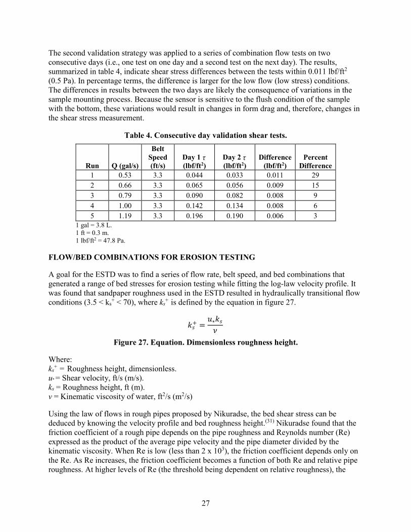
The second validation strategy was applied to a series of combination flow tests on two consecutive days (i.e., one test on one day and a second test on the next day). The results, summarized in table 4, indicate shear stress differences between the tests within 0.011 lbf/ft2 (0.5 Pa). In percentage terms, the difference is larger for the low flow (low stress) conditions. The differences in results between the two days are likely the consequence of variations in the sample mounting process. Because the sensor is sensitive to the flush condition of the sample with the bottom, these variations would result in changes in form drag and, therefore, changes in the shear stress measurement.

Table 4. Consecutive day validation shear tests.

Run Q (gal/s)

Belt Speed (ft/s)

Day 1 (lbf/ft2)

Day 2 (lbf/ft2)

Difference (lbf/ft2)

Percent Difference

1 0.53 3.3 0.044 0.033 0.011 29 2 0.66 3.3 0.065 0.056 0.009 15 3 0.79 3.3 0.090 0.082 0.008 9 4 1.00 3.3 0.142 0.134 0.008 6 5 1.19 3.3 0.196 0.190 0.006 3

1 gal = 3.8 L. 1 ft = 0.3 m. 1 lbf/ft2 = 47.8 Pa.

FLOW/BED COMBINATIONS FOR EROSION TESTING

A goal for the ESTD was to find a series of flow rate, belt speed, and bed combinations that generated a range of bed stresses for erosion testing while fitting the log-law velocity profile. It was found that sandpaper roughness used in the ESTD resulted in hydraulically transitional flow conditions (3.5 < ks

+ < 70), where ks+ is defined by the equation in figure 27.

Figure 27. Equation. Dimensionless roughness height.

Where: ks

+ = Roughness height, dimensionless. u* = Shear velocity, ft/s (m/s). ks = Roughness height, ft (m). ν = Kinematic viscosity of water, ft2/s (m2/s)

Using the law of flows in rough pipes proposed by Nikuradse, the bed shear stress can be deduced by knowing the velocity profile and bed roughness height.(31) Nikuradse found that the friction coefficient of a rough pipe depends on the pipe roughness and Reynolds number (Re) expressed as the product of the average pipe velocity and the pipe diameter divided by the kinematic viscosity. When Re is low (less than 2 x 103), the friction coefficient depends only on the Re. As Re increases, the friction coefficient becomes a function of both Re and relative pipe roughness. At higher levels of Re (the threshold being dependent on relative roughness), the

τ τ

𝑘𝑘𝑠𝑠+ =𝑢𝑢∗𝑘𝑘𝑠𝑠𝜈𝜈

27

friction coefficient depends only on the relative pipe roughness. For turbulent flow in rough pipes, Nikuradse provided the velocity distribution function seen in figure 28:

Figure 28. Equation. The law of the wall.

Where: u = Velocity at a depth, y, ft/s (m/s). u* = Shear velocity, ft/s (m/s). κ = Von Karman constant, 0.4. y = Depth at which the velocity, u, is taken, ft (m). B = Constant depending on the dimensionless roughness height, ks

+.

Although Nikuradse conducted experiments in circular pipes, the velocity function can be extended to flow along a plate, a streamline body, a rectangular pipe, or an open channel. The velocity function is then called the universal law of the wall. For flows in the ESTD, the conduit flow condition can be considered similar to that of Nikuradse’s experiments except that the ESTD test channel does not have identical roughness on all of the boundaries. The belt roughness is much larger than that of the test channel bed. The effect of this difference will vary with the belt speed.

As stated at the beginning of this section, the goal was to find combinations of discharge, belt speed, and bed roughness that recreated the log-law velocity profile. When the belt speed is too low or too high, the influence of belt roughness will extend to very close to the test channel bed, which in turn may limit the application of the law of the wall to a very small height above the bed. Such a limited depth would make fitting observed and theoretical values of velocity nearly impossible.

A four-step procedure was used to identify the combinations appropriate for ESTD testing.

Step 1: Calculate the Bed Roughness with the Measured Shear Stress of the Conduit Flows

The measured shear stresses were considered to be accurate. The friction coefficient, f, was then calculated by the equation in figure 29.

Figure 29. Equation. Friction coefficient.

Where: f = Friction coefficient. τ = Shear stress, lbf/ft2 (Pa). ρ = Density of water, lb/ft3 (kg/m3).

= Average velocity, ft/s (m/s).

𝑢𝑢𝑢𝑢∗

= 5.75𝑙𝑙𝑙𝑙𝑔𝑔 �𝑦𝑦𝑘𝑘𝑠𝑠� + 𝐵𝐵 =

1𝜅𝜅𝑙𝑙𝑙𝑙 �

𝑦𝑦𝑘𝑘𝑠𝑠� + 𝐵𝐵

𝑓𝑓 =8𝜏𝜏𝜌𝜌𝑈𝑈�2

𝑈𝑈�

28

Nikuradse provides relationships between f, r, ks, and ks+ for different values of log(ks

+) as listed in table 5.(31) The equivalent circular radius for the rectangular conduit, r, is calculated by r = 2A/P, where A is the cross-sectional area and P is the wetted perimeter. With known f, a roughness height, ks, can be calculated based on the relationships in table 5.

Table 5. Relationship between f, r, ks, and ks+.

Value of log(ks+) Relationship between f, r, ks, and ks+

It was found that for a specific sandpaper grade, the calculated roughness height varied with flow rate. The reasons for this may include the following: 1) the fact that only the test channel bed (not the sides and top) was lined with sandpaper, and the calculation assumes identical roughness across the cross section of the test channel; and 2) the uncertainty in measuring the bed shear stress. For each sandpaper grade, the average roughness height was used in the subsequent analyses. Table 6 summarizes the roughness heights for the bed conditions.

Table 6. Particle size and modeled roughness height.

Bed Material

Average particle size, D50 (inches)

Average particle size, D50

(mm)

Roughness Height, ks (inches)

Roughness Height, ks

(mm) ks/D50 Plexiglass™ N/A N/A 0.0101 0.257 N/A P320 sandpaper 0.0018 0.045 0.0109 0.277 6.2

P220 sandpaper 0.0027 0.068 0.0128 0.325 4.8

P150 sandpaper 0.0039 0.100 0.0128 0.326 3.3

P100 sandpaper 0.0064 0.162 0.0156 0.395 2.4

P80 sandpaper 0.0079 0.200 0.0195 0.496 2.5 N/A = Not applicable.

log(𝑘𝑘𝑠𝑠+) ≤ 0.55 1

�𝑓𝑓− 2log �

𝑟𝑟𝑘𝑘𝑠𝑠� = 0.8 + 2log�𝑘𝑘𝑠𝑠

+�

0.55 ≤ log�𝑘𝑘𝑠𝑠+� ≤ 0.85 1


𝑟𝑟𝑘𝑘𝑠𝑠� = 1.18 + 1.13log�𝑘𝑘𝑠𝑠

+�

0.85 ≤ log�𝑘𝑘𝑠𝑠+� ≤ 1.15 1

�𝑓𝑓− 2 log �

𝑟𝑟𝑘𝑘𝑠𝑠� = 2.14

1.15 ≤ log�𝑘𝑘𝑠𝑠+� ≤ 1.83 1


𝑟𝑟𝑘𝑘𝑠𝑠� = 2.81 − 0.588log�𝑘𝑘𝑠𝑠

+�

1.83 ≤ log�𝑘𝑘𝑠𝑠+� 1

�𝑓𝑓− 2 log �

𝑟𝑟𝑘𝑘𝑠𝑠� = 1.74

29

The roughness height is larger than average particle size of the bed sandpaper as shown in the last column of the table. In Nikuradse’s experiments, uniform sand particles were glued to the inner surface of the pipes. Two layers of lacquer were applied to the sands to provide a strong bond. This reduced the effective particle size somewhat, so that the effective roughness was also smaller. Although Nikuradse used average particle size as the relevant roughness height, some have proposed the use of 2.5 or larger multipliers on the actual particle size to determine the effective bed roughness height.

Step 2: Validate the Bed Roughness by Predicting Conduit Flow Velocity Profiles

The roughness height was validated by predicting conduit flow velocity profiles using the equation in figure 28. Nikuradse provided relations to calculate the constant B, which are listed in table 7.(31) The constant, B, is calculated using the roughness height determined in step 1 and the shear velocity calculated from the measured shear stress. The velocity profile of the lower half of the flow field of the rectangular conduit flow—as shown in figure 19, for example—can be predicted.

Table 7. Equations for the constant B.

Value of log(ks+) Equation for B

The predicted velocity profile is then compared with the measured velocity profile. For example, figure 30 summarizes a comparison of measured and predicted conduit flow velocities for the P220 sandpaper bed for a range of flow rates. The difference between the measured and predicted velocity on all sandpaper beds evaluated was within -7 and 3 percent, demonstrating that the velocity can be predicted by the roughness height estimated from shear stress measurements.

log�𝑘𝑘𝑠𝑠+� ≤ 0.55 B = 5.5 + 5.75log(ks+)

0.55 ≤ log�𝑘𝑘𝑠𝑠+� ≤ 0.85 B = 6.59 + 3.5log(ks+)

0.85 ≤ log�𝑘𝑘𝑠𝑠+� ≤ 1.15 𝐵𝐵 = 9.58

1.15 ≤ log�𝑘𝑘𝑠𝑠+� ≤ 1.83 𝐵𝐵 = 11.5 − 1.62log�𝑘𝑘𝑠𝑠

+� 1.83 ≤ log�𝑘𝑘𝑠𝑠

+� 𝐵𝐵 = 8.48

30

1 inch = 25.4 mm. 1 gal = 3.8 L.

Figure 30. Graph. Comparison of conduit flow point velocities on a P220 sandpaper bed.

Step 3: Fit the Shear Velocity of Flow Conditions with Both the Pump and Belt Running

After validation, the roughness height calculated in step 1 is used to predict the velocity profiles for flow conditions when both the belt and pump are running. By fitting measured velocity data to the equation in figure 28, the shear velocity can be fitted, and, therefore, the wall shear stress can be calculated. The constant B is calculated by the relations in table 7.

Step 4: Identify the Flow Conditions for ESTD Testing

Flow conditions with equivalent fitted (step 3) and measured shear stresses and velocity profiles over the entire flow depth that approximate the log-law velocity profile were identified by comparing velocity predictions from the equation in figure 28 with measured velocity data. Those conditions providing a match were used for testing soil samples in the ESTD.

A series of seven test conditions whose velocity profiles follow the log-law profile and result in the desired range of shear stress conditions were identified. Figure 31 illustrates the measured velocity data compared to the law of the wall for the selected conditions. The discrete symbols in the figure represent the measured velocity points. The curves shown are composed of three parts. When the dimensionless flow depth, y+, is greater than 30, the curve is the fitted log-law equation. When the dimensionless flow depth, y+, is less than 5, the curve represents the Newton shear stress equation, u = y/ . In this equation, is the bed shear stress, y is flow depth, and is the dynamic viscosity of water. A linear relation is estimated between the upper end of the range of y+ covered by the Newton shear stress and the lower end of the range of y+ covered by the log-law equation.

20

40

60

80

20 40 60 80

Pred

icte

d p

iont

vel

ociti

es (i

nche

s/s)

Measured point velocities (inches/s)

Conduit flow rate of 0.53 gal/sConduit flow rate of 0.66 gal/sConduit flow rate of 0.79 gal/sConduit flow rate of 0.92 gal/sConduit flow rate of 1.06 gal/s

τ µ τ µ

31

The velocity profile corresponding to a shear stress of 0.15 lbf/ft2 (7.2 Pa) is an example of a profile where nearly the entire velocity profile corresponds to the law of the wall. These seven conditions indicate that the ESTD can model the very near-bed flow condition of an open-channel flow given a specific wall shear stress and bed roughness.

In each of the seven cases, the computed shear stress matches the measured shear stress that is shown on the figure. The fitted parameters and shear stress for each condition is summarized in table 8. All erosion tests were conducted using one of these combinations of flow rate, belt speed, and bed roughness.

1 ft = 0.3 m. 1 gal = 3.8 L. 1 inch = 25.4 mm.

Figure 31. Graph. Conditions used for erosion testing in the ESTD.

0.0

0.2

0.4

0.6

0.8

0 20 40 60 80 100

y (inc

hes)

V (inches/s)

0.056 lbf/ft20.314 lbf/ft2

0.273 lbf/ft2

0.209 lbf/ft20.150 lbf/ft2

0.102 lbf/ft20.075 lbf/ft2

32

Table 8. Test conditions for the ESTD.

Bed Sandpaper

Flow, gal/s (L/s)

Belt Speed,

ft/s (m/s)

Measured Bed Shear

Stress, lbf/ft2 (Pa)

Fitted Bed Shear Stress,

lbf/ft2 (Pa) P80 0.58 (2.2) 3.3 (1) 0.056 (2.7) 0.063 (3.0) P150 0.66 (2.5) 3.3 (1) 0.075 (3.6) 0.073 (3.5) P150 0.79 (3.0) 3.3 (1) 0.102 (4.9) 0.108 (5.2) P320 1.02 (3.9) 6.6 (2) 0.150 (7.2) 0.150 (7.2) P150 1.11 (4.2) 6.6 (2) 0.209 (10.0) 0.188 (9.0) P100 1.19 (4.5) 6.6 (2) 0.273 (13.1) 0.235 (11.3) P80 1.19 (4.5) 3.3 (1) 0.314 (15.0) 0.308 (14.8)

33

CHAPTER 5. SOIL PREPARATION AND PROPERTIES

This chapter describes the preparation of soil specimens for testing in the ESTD and soil properties determined from standard testing protocols.

PREPARATION OF SOIL SPECIMENS

Soil specimens must be prepared so that they will maintain their shape prior to the initiation of erosion in the ESTD. With some approaches to soil preparation in a laboratory, the specimens will slake in water. (See appendix C for a description of slaking.) Because slaking is a completely different mechanism for soil loss than the erosion process, slaking should be avoided.

Soil Preparation by Compaction

Traditional geotechnical preparation of soil specimens follows procedures from the standard compaction test (ASTM D698). This protocol requires that a moisturized clay mixture matures for a minimum of 16 h before it is compacted in a standard 4-inch (100-mm)-diameter mold. Next, a 5.5-lb (2.5-kg) hammer is dropped for 25 blows per lift on three separate lifts. This compaction approach is appropriate for many geotechnical applications at low water contents.

In the wet environment in which erosion tests are conducted, a soil specimen prepared in this way immediately slakes and releases air bubbles into the water. This phenomenon is not observed in the field. Therefore, preparation of soils for erosion testing by this approach is not appropriate. Moreover, when a soil mixture is too plastic, as are many of the cohesive soils of interest in this study, it adheres to the hammer and makes compaction difficult.

Some investigators have attempted to address this limitation. In one study, Red Art Kaolin clay specimens were prepared using a consolidometer cell in air.(32) Like the compaction method, use of a consolidometer shortens the preparation time. However, if the extruded clay specimen is immediately immersed in water, then it slakes and releases air bubbles. Subsequent soil preparation attempts included leaving the specimens in a closed zip bag for 2 h. In this case, soils demonstrated a somewhat greater resistance to slaking. However, the soil was eventually affected by slaking.

This behavior has been described as resulting from the swelling and bursting of pressurized air bubbles formed during consolidation. The swelling and bursting destroys the connections among soil particles and causes the soil to collapse.(33) If pressurized air bubbles account for the slaking of specimens, then it is vital to eliminate them during the soil preparation process. Therefore, vacuum extraction of the trapped air is desired. A pugger mixer serves this purpose.

Soil Preparation with a Pugger Mixer

A pugger mixer is commonly used in pottery studios. It features a vacuum pump for de-airing the mixing chamber. The pugger mixer at the Hydraulics Lab in the Turner Fairbank Highway Research Center can pug out 3-inch (76-mm)-diameter cohesive soil specimens after sufficient mixing. A 2.5-inch (63.5-mm) cutting ring was used to prepare 2.5-inch (63.5-mm)-diameter soil specimens. Figure 32 is a picture of the pugger mixer pugging soil.

35

The pugger mixer is capable of mixing sands with a maximum particle size of 0.20 inches (5 mm). Clay, commercial silt, and non-uniform sands in varied percentages can be mixed into cohesive soils with a range of characteristics. Soil specimens prepared with the pugger mixer do not slake in water, which is necessary for testing the erosion characteristics of the soil specimens under water.

Figure 32. Photo. The pugger mixer used for soil preparation.

Soil Composition and Classification

All cohesive soil specimens prepared for erosion testing in the ESTD contained mixtures of Red Art clay, commercial silt, and non-uniform sands with specific gravities of 2.80, 2.63, and 2.69, respectively. The Red Art clay contains 40 percent Illite, 27 percent chlorite, and 28 percent quartz. The chemical components are mainly SiO2 (61.3 percent) and Al2O3 (17.6 percent).

None of the three component soil materials are well graded, as summarized in figure 33. The particle size ranges are as follows:

• Red Art clay ranges from 0.002 inches (0.05 mm) to less than 0.00004 inches (0.001 mm).

• Silt ranges from 0.003 inches (0.075 mm) to 0.00008 inches (0.002 mm).

• Non-uniform sand: 0.20 inches (5 mm) to 0.003 inches (0.075 mm).

As defined by ASTM D2487-10, sands are those particles that will pass a No. 4 sieve (0.19 inches (4.75 mm)) and be retained on a No. 200 sieve (0.003 inches (0.075 mm)). Fines—clays and silts—are those particles that pass the No. 200 sieve (0.003 inches (0.075 mm)). The distinction between clays and fines further relates to their PI and liquid limit (LL). Soil specimens were classified according to the ASTM standard D2487-10. It classifies inorganic fine-grained soils into five categories based on the LL and PI of a soil. The LL, plastic limit (PL), and PI, also known as the Atterberg limits, apply only to the portion of a soil that passes the No. 40 sieve (0.017 inches (0.425 mm)).

36

25.4 mm = 1 inch.

Figure 33. Graph. Particle-size distributions for Red Art clay, silt, and non-uniform sands.

Six types of soils were prepared for the ESTD erosion tests with different proportions of the Red Art clay, silt, and non-uniform sand. Table 9 summarizes the component mixtures, soil classification, and general grain size properties for the soils. They are categorized in the broad classifications of CL and CL-ML.

The particle-size distributions of these six soils are provided in figure 34. All six soils are gap graded because none of three components was well-graded.

Table 9. Classification and composition of soils for testing.

Soil Index

Soil Classification

Source Mix (%) Fraction (%) Specific Gravity

Plastic Limit (%)

Liquid Limit (%)

Plasticity Index (%)

Red Art Silt Sands < 2 m < 50 m < 75 m < 425 m

1 CL-ML (sandy silty clay) 20 40 40 8.1 58.9 60.6 77.2 2.69 16.7 21.0 4.3

2 CL (sandy lean clay) 30 20 50 9.5 49.5 50.7 71.5 2.71 14.3 21.3 7.0

3 CL (sandy lean clay) 40 10 50 11.5 49.7 50.7 71.5 2.73 14.4 24.1 9.7

4 CL-ML(Silty

clay with sand)

25 45 30 9.8 68.8 70.4 82.9 2.69 17.4 22.5 5.1

5 CL (Lean clay with sand) 40 40 20 13.5 78.9 80.3 88.6 2.71 17.7 26.4 8.7

6 CL (Lean clay with sand) 40 30 30 12.9 69.2 70.4 82.9 2.72 16.6 25.5 8.9

0%

10%

20%

30%

40%

50%

60%

70%

80%

90%

100%

0.0010.0100.1001.00010.000

Perce

nt fin

er

Particle diameter (mm)

SandSiltRed Art

µ µ µ µ

37

25.4 mm = 1 inch.

Figure 34. Graph. Particle-size distributions of the cohesive soils tested in the ESTD.

Each soil mixture was prepared with a range of water contents to create 17 unique soil samples for testing. Three additional unique soil samples were prepared by the compaction method. All soil specimens were prepared in the shape of a cylinder with a diameter of 2.5 inches (63.5 mm) and a height of 0.79 inches (20 mm).

To prepare the soil samples, the previously specified mixes of dry Red Art clay, silt, and sand were thoroughly mixed. Distilled water was added gradually to achieve a uniform soil texture. The mixture was pugged out and cured for 16 h. After the curing, the mixture was remixed in the pugger. It was then vacuumed near the end of mixing. Finally, the soil was pugged out, cut to the desired size, and saved in water before the erosion test. If a soil mixture was too wet, then it would slip in the pugger chamber and could not be pugged out.

The water content (weight of water divided by weight of soil) and the dry bulk density were measured. The wet bulk density, void ratio, and saturation degree were calculated. Table 10 summarizes the properties of the soil samples prepared by the pugger mixer. The soil sample name is in the form of xWyyy, where “x” represents the soil index and “yyy” represents the measured water content without the decimal point.

For comparison, three soil samples were compacted following the procedures of the compaction test (ASTM 698-00a). These samples all had lower water contents than those prepared by the pugger mixer. After the soil specimen was prepared, it was saved in a closed zip bag for 2 h before the erosion test. Table 11 summarizes the properties of the soil samples prepared by compaction.

38

Table 10. Mass and moisture properties of soils prepared by pugger mixer.

Soil Index

Soil Sample

Measured Water

Content, w (%)

Wet Bulk

Density (lb/ft3)

Wet Bulk

Density (kg/m3)

Dry Bulk

Density (lb/ft3)

Dry Bulk

Density (kg/m3)

Void Ratio, e (%)

Degree of Saturation,

S (%) 1 1W156 15.6 134.4 2,155 116.3 1,865 44.2 94.6 1 1W165 16.5 134.4 2,156 116.3 1,865 44.2 94.9 1 1W181 18.1 129.9 2,084 110.1 1,765 52.4 92.8 2 2W147 14.7 135.7 2,177 118.3 1,898 42.8 93.1 2 2W167 16.7 137.0 2,197 117.2 1,880 44.1 103.5 2 2W177 17.7 138.1 2,214 117.0 1,876 44.5 109.8 3 3W160 16.0 134.6 2,159 116.2 1,864 46.5 93.0 3 3W180 18.0 136.0 2,181 115.0 1,845 48.0 103.6 4 4W189 18.9 131.0 2,101 110.3 1,769 52.1 97.0 4 4W198 19.8 130.1 2,086 108.8 1,745 54.2 97.1 4 4W217 21.7 130.1 2,087 106.8 1,713 57.0 103.0 5 5W215 21.5 130.0 2,085 107.1 1,717 57.8 100.4 5 5W231 23.1 126.6 2,031 102.8 1,649 64.3 97.6 5 5W248 24.8 126.8 2,033 101.7 1,631 66.2 101.0 6 6W192 19.2 132.1 2,119 111.2 1,783 52.6 97.5 6 6W200 20.0 129.6 2,078 108.1 1,733 57.0 95.1 6 6W231 23.1 130.0 2,085 105.8 1,697 60.3 103.2

Table 11. Mass and moisture properties of soils prepared by compaction.

Soil Index

Soil Sample

Measured Water

Content, w (%)

Wet Bulk

Density (lb/ft3)

Wet Bulk

Density (kg/m3)

Dry Bulk

Density (lb/ft3)

Dry Bulk

Density (kg/m3)

Void Ratio, e (%)

Degree of Saturation,

S (%) 1 1W133 13.3 131.0 2,101 115.9 1,858 44.8 78.6 2 2W127 12.7 130.3 2,090 115.5 1,853 46.2 74.9 3 3W126 12.6 132.8 2,129 117.8 1,889 44.5 77.9

ADDITIONAL GEOTECHNICAL PROPERTIES

Additional geotechnical properties of the soils were measured in accordance with the applicable ASTM standards. These properties included drained cohesion, friction angle, and unconfined compression strength.

Direct Shear Test

The direct shear test measures the cohesion and friction angle of a soil. Cylindrical soil specimens with a diameter of 2.5 inches (63.5 mm) and a height of 1 inch (25.4 mm) were used in the direct shear test. The soil specimens were identical to those for the ESTD erosion test except that the cylinders were shorter. During the direct shear test, 0.5-inch (12.7-mm) shear displacement was achieved within either 50 or 75 min. Four normal stresses—5, 10, 20, and 30 lbf/inches2 (34, 69, 138, and 207 kPa)—were used. Test results for the soils prepared using the pugger mixer are found in table 12, while those prepared by compaction are found in

39

table 13. For the same soil index, soils prepared by compaction exhibited higher values of cohesion than soils prepared by the pugger mixer.

Table 12. Additional geotechnical properties of soils prepared by pugger mixer.

Soil Index

Soil Sample

Cohesion, c (lbf/inches2)

Cohesion, c (kPa)

Friction Angle,

(◦)

Unconfined Compressive Strength, qu

(lbf/ft2)

Unconfined Compressive Strength, qu

(Pa) 1 1W156 1.01 6.96 37.2 2,378 113,764 1 1W165 1.23 8.48 35.9 2,162 103,421 1 1W181 1.14 7.86 37.3 1,661 79,497 2 2W147 0.58 4.03 38.6 3,961 189,537 2 2W167 1.42 9.79 37.6 1,000 47,850 2 2W177 0.72 4.96 38.7 1,009 48,263 3 3W160 0.92 6.36 36.3 1,723 82,461 3 3W180 1.03 7.10 36.3 1,216 58,192 4 4W189 1.15 7.93 37.4 2,144 102,594 4 4W198 0.74 5.10 39.8 1,242 59,433 4 4W217 1.30 8.96 37.7 990 47,367 5 5W215 1.29 8.89 35.3 3,012 144,100 5 5W231 1.12 7.72 35.2 1,366 65,362 5 5W248 1.04 7.17 36.1 1,055 50,470 6 6W192 3.32 22.89 27.8 3,373 161,406 6 6W200 1.26 8.69 31.8 1,636 78,256 6 6W231 1.42 9.79 32.5 993 47,505

Table 13. Additional geotechnical properties of soils prepared by compaction.

Soil Index

Soil Sample

Cohesion, c (lbf/inches2)

Cohesion, c (kPa)

Friction Angle,

(◦) 1 1W133 2.63 18.13 37.4 2 2W127 2.42 16.69 34.9 3 3W126 1.24 8.55 35.8

Unconfined Compression Test

Based on laboratory testing and field observation on 12 channels in 6 western States, Flaxman concluded that the unconfined compressive strength was an indicator of soil resistance to erosion.(34) He defined a linear relationship between tractive stream power (product of flow-induced shear stress and flow velocity) and the logarithm of the unconfined compressive strength that could be used to separate conditions in eroding versus stable channels. The R2 value of this relation was 0.4. Straub and Over found a linear relationship between soil critical shear stress and the logarithm of unconfined compressive strength in 15 field cohesive soils in Illinois.(8) The R2 value of this relation was 0.95. In their study, the critical shear stress of undisturbed field soil specimens were deduced from erosion results in the EFA.

φ

φ

40

Because of these findings, unconfined compressive strength was determined for each of the soil samples. Cylindrical soil specimens with a diameter of 2.5 inches (63.5 mm) and a height of 6 inches (152 mm) were used in the test. The soil specimens were identical to those for the ESTD erosion test except that the cylinders were longer. Test results for the soils prepared using the pugger mixer are found in table 12.

SLAKING

Slaking is a soil loss mechanism that should be avoided by proper preparation of test specimens for erosion testing. Slaking results in soil loss even without the shear stresses of flowing water and results in accelerated erosion rates from what would be expected in the absence of slaking.

The Slaking Mechanism

Berghager and Ladd defined slaking as the progressive breaking-up of a soil when immersed in water.(33) The break-up of the soil is accompanied by the release of small air bubbles. Higher degrees of saturation means less air is present and makes a soil less vulnerable to slaking. Slaking results in soil loss but from a completely different mechanism than erosion caused by bed shear stresses.

Although the actual mechanism of slaking is not well understood, it is generally accepted that the slaking of cohesive soil is because of air pressure change in the soil capillaries.(16) When a wet unsaturated soil is soaked in water, the dipolar water molecules are attracted by the clay particles, and thus the water moves into the pores. Water forms menisci within the pores, which compress air in the soil pores. The entrapped air exerts enormous pressure, which breaks the tensile strength of the soil and explains why slaking is always accompanied by the release of air bubbles. In addition, because the capillary menisci pull water into the pores, the capillary walls are in tension. If the tensile strength of the pore walls is less than the tension applied by the menisci, then the walls will fracture and the soil will break up.(35)

Researchers have experimentally demonstrated the significance of slaking in compacted soils using the CCFED.(36) Others have identified four slaking modes: dispersion slaking, swelling slaking, body slaking, and surface slaking.(37)

Excluding surficial layers of mud containing significant quantities of microorganisms, such as snails, river bed soils near bridge piers are anticipated to be well compacted and saturated. Therefore, it is realistic to assume those soils are free of slaking. To reproduce these conditions in a laboratory, prepared soil specimens must also be free of slaking in order to study their erosion characteristics. However, most tested soil specimens in laboratories are prepared by the method outlined in the standard ASTM compaction test, which rarely prepares soils that will not slake.(33,36,38)

Researchers working with the CCFED identified slaking as a concern, noting that samples made directly in the mold contained air voids and cracks.(38) To remedy this problem, a Vac-Aire extruding machine was used to remove air from the soil. Others concluded that compacted soil cannot be tested in the CCFED, although no reason was given.(16)

41

In general, however, slaking of compacted soils has not been widely recognized for the following reasons:

1. Compacted soils are seldom tested underwater where slaking occurs.

2. Previous erosion testing devices, including EFA and HET, constrain the sides of soil specimens. The EFA specimens are confined in Shelby tubes, while the HET testing soils are confined in cylindrical containers.

Constraining compacted soil specimens may delay slaking. If exposed to water for a sufficient time, a soil specimen inside a Shelby tube may slake and generate cracks, which means that the erosion test measurements will not be accurate unless the test is sufficiently short enough that slaking is not allowed to begin.

Researchers tested field and laboratory compacted New Orleans levee soils with the EFA.(39) The field samples (labeled S2) and the laboratory samples (labeled S4) are summarized in table 14. The two laboratory soils were compacted with different levels of effort. The low compaction effort was 920 ft-lbf/ft3 (44 kN-m/m3), which is 1.6 percent of the modified Proctor compaction effort (ASTM D1557). The high compaction effort was 56,200 ft-lbf/ft3 (2700 kN-m/m3), which is 100 percent of the modified Proctor compaction effort. (The saturation degree is calculated by assuming that the soil specific gravity is 2.65. Because S2-B1 contains nearly 17 percent organic content, the saturation estimate is an underestimate. It is likely that the saturation degree of S2-B1 approaches 100 percent.)

Table 14. Properties of four soils from a New Orleans levee.

Sample Soil

Type

Wet Specific Weight (lbf/ft3)

Dry Specific Weight (lbf/ft3)

Organic Content

(%)

Water Content

(%)

Liquid Limit (%)

Plastic Limit (%)

Plasticity Index (%)

Saturation Degree

(%) S2-B1-(0-2ft)-TW CL 126 108 16.94 16.11 46 17 29 81

S2-B2-(2-4ft)-SW CL 129 106 1.62 21.23 41 16 25 100

S4-(0-0.5ft)-LC-

SW CL 88 66 8.16 33.14 60 30 30 59

S4-(0-0.5ft)-HC-

SW CL 113 84 8.16 33.14 60 30 30 93

Figure 35 summarizes the EFA erosion testing results for the levee soils. The S4 (low compaction) soil has the lowest degree of saturation and, therefore, the most air bubbles. It also exhibits the highest erosion rates of the four tested soils. Conversely, the highly compacted S4 soil, with a much higher degree of saturation, exhibits the lowest erosion rates in line with the field soils. The erosion rates differed by over four orders of magnitude. The high compaction effort may have eliminated more air mimicking the field conditions, while the low compaction effort merely trapped and pressurized the air.

42

Figure 35 also indicates that the erosion rates of the highly compacted S4 soils are close to that of both prototype S2 soils when flow velocities are greater than 8 ft/s (2.4 m/s). Below that velocity, S2 soils exhibit minimal erosion rates. However, the highly compacted S4 soils have somewhat larger erosion rates (0.02 inches/h (0.4 mm/h)) at the flow velocity of 2.6 ft/s (0.8 m/s). This might be explained by slaking. When flow velocities exceed 8 ft/s (2.4 m/s), erosion is more dominant than slaking. Several researchers have considered whether gradation influences slaking behavior.

One research effort compared compacted clay and sand mixtures prepared in the laboratory with field-collected cohesive soils compacted in the laboratory.(36) These included well and poorly graded soil samples.

Another study assessed a well-graded reconsolidated Boston Blue clay with an LL of 30 percent and a PL of 17.5 percent.(33) Most of the Boston Blue clays were reconsolidated with a low compaction effort of approximately 2,100 ft-lbf/ft3 (100 kN-m/m3). The standard compaction test (ASTM D698) applies a compaction effort of 12,400 ft-lbf/ft3 (600 kN-m/m3).

Another study evaluated a well-graded Texas lean clay with an LL of 47 percent and a PL of 21 percent.(38) The gradations for the latter two clays are shown in figure 36. None of these assessments suggested that soil gradation plays a significant role in slaking.

1 ft = 0.3 m. 1 inch = 25.4 mm. 1 kPa = 0.15 psi.

Figure 35. Graph. Erosion curves of soils from a New Orleans levee.

43

It may be concluded that lower compaction efforts contribute to slaking because these soils contain pressurized air bubbles. These air bubbles will release pressure once the soil becomes unconstrained. This process might happen in a quick or slow burst into the soil inner structure, which leads to small disconnected cracks in the soil structure. With the existence of water, the air pressure increases, and stronger bursts occur, creating still more cracks. Once the cracks are connected, the water easily penetrates into and breaks up the soil. Much higher compaction efforts are needed to actually force the air out of the sample.

Once a soil sample prone to slaking is immersed in water, the potential for slaking is likely to increase the longer the sample is submerged. Therefore, if such a sample must be tested for its erosion properties, then the test should be conducted as quickly as possible. However, this process does not guarantee a meaningful result. Generally, compaction methods cannot be used in preparing soils for erosion testing. Soils should be vacuumed in their preparation to eliminate trapped pressurized air and, therefore, slaking.

1 m = 0.00003937 inches.

Figure 36. Graph. Gradation of compacted clays.

Slaking Test

The soil samples prepared by compaction in this study were evaluated for slaking to generate quantitative information regarding the slaking phenomenon. The compaction effort applied was 12,400 ft-lbf/ft3 (600 kN-m/m3) per ASTM D698. The cylindrical test specimens had a diameter of 2.5 inches (63.5 mm) and a height of 1 inch (25.4 mm). Properties of these soil samples are summarized in table 11 and table 13.

0%

10%

20%

30%

40%

50%

60%

70%

80%

90%

100%

110100

Perce

nt fin

er

Particle diameter (µm)

Boston Blue clayTexas lean clay

µ

44

The samples were placed in an aluminum tray and suspended beneath a balance. The soil extended above the rim of the tray so that the top 0.28 inches (7 mm) was unconfined. The samples were then submerged in still water for a duration of at least 1 h. After soaking in water, cracks appeared on the surface of the soil specimen. Air bubbles were released from inside of the soil specimen. The soil started to crumble until a stable condition was reached. The soil sample was removed from water and typically appeared as shown in figure 37.

The initial and final soil masses were measured as well as the total mass of the aluminum tray and wire when empty. Continuous balance readings were recorded after submergence through the end of the test. Figure 38 summarizes three sets of slaking data for soil indices 2 and 3. All three slaking curves have an S-shape. Initially, the slaking was slow, but after several minutes, the rate of soil loss increased. After about 30 min, the slaking rate slowed until no further soil loss was observed. The final shape of the remaining soil was that of the frustum of a cone. The slaking curve can be approximated by a hyperbolic tangent function as shown in figure 38. The two constants should be functions of soil composition, compaction effort, and sample size.

Figure 37. Photo. Slaking test on a compacted soil specimen.

45

1 oz = 28.3 g.

Figure 38. Graph. Slaking test results for soils 2 and 3 in still water.

These tests demonstrated that over the hour-long test periods anticipated for erosion testing in the ESTD, slaking would be a significant contributor to the soil loss. Therefore, the soil samples prepared using the standard compaction effort (ASTM D698) could not be used for erosion testing.

Slaking of soil III-1

46

CHAPTER 6. EROSION TESTING PROTOCOL AND RESULTS

All erosion tests in the ESTD were conducted by applying one or more of the seven combinations of flow, moving belt speed, and bed roughness that reproduced open channel flow conditions to each of the 17 soil types in table 10. Distilled water was used in the ESTD system.

For testing, each soil specimen was placed in an aluminum tray with sides extending up 0.5 inches (13 mm). The remaining 0.28 inches (7 mm) of the cylindrical soil sample is unconfined and available for erosion. The tray is fixed onto the sensor disk of the force gauge. Initially, the surface of the soil specimen is flush with the bed of the test channel. The sensor disk and soil specimen are elevated as erosion occurs to maintain this flush condition. Initial roughness of the soil specimen is carefully prepared so that it is similar to the bed roughness of test channel. When successful in matching the roughness, the initial average shear stress on the soil specimen should approximate the bed shear stress.

During each erosion test, the measured bed shear stress under each flow condition should be maintained as a constant. As erosion occurs, the measured shear stress would decrease if the specimen is held at a fixed position. Therefore, the specimen is automatically raised when the measured shear stress decreases below the target value so that the remaining surface of the soil sample is flush with the fixed bed.

Raising the specimen is controlled by a feedback loop on the force gauge. A shear stress range of 0.021 lbf/ft2 (1 Pa) is applied to determine whether the soil specimen should be elevated. Readings are checked every 2 s. If the shear stress dropped by more than the allowable amount, then the platform is elevated for an increment of time referred to as the elevation period. The elevation period varies depending on the erodibility of the soil specimen. Rapidly eroding soil specimens require longer elevation periods compared with more slowly eroding soil specimens. Because any protrusion or depression will introduce form drag and potentially alter the erosion patterns, these measures are important to reduce the potential for form drag.

A typical set of recorded instantaneous shear stress measurements is plotted in figure 39. The instantaneous shear stress fluctuated around the target bed shear stress of 0.31 lbf/ft2 (15 Pa). The figure also shows the elevation increases of the platform and soil sample. The soil elevation curve can be approximated with a linear function. The slope of the function, in units of depth versus time, represents one estimate of the erosion rate.

Each erosion test is typically run for approximately 1 h, but the time is adjusted depending on the erosion rate. The initial and final soil masses are measured. The mass loss is divided by the erosion time to calculate a mass erosion rate (mass per unit time). This mass erosion rate is divided by the surface area of the soil sample to derive a more useful mass erosion rate per unit area.

Water content of several soils was measured again after the 1-h test. Water content increased by less than 0.5 percent for soils prepared in the pugger mixer. The water content increased by approximately 2 percent for the compacted soils. Therefore, for soils prepared in the pugger mixer, the wet density did not change significantly. Because of this result, the total eroded soil

47

volume can be calculated along with a depth-based erosion rate. This results in an erosion rate in depth per unit time.

1 inch = 25.4 mm. 1 lbf/ft2 = 47.8 Pa.

Figure 39. Graph. Example data recorded for sample with soil index 4.

Erosion of soils prepared with the pugger mixer was in a form of soil lumps and cloudy matter. When bed shear stress was small, the primary erosion mechanism was the separation of soil lumps from the surface. The lumps were entrained from all areas of the soil surface, resulting in an irregular soil surface over time. As the bed shear stress increased, the cloudy matter appeared heavier. Figure 40 shows this change for soil sample 1W181. For the lower bed shear stress of 0.10 lbf/ft2 (4.9 Pa), there was no cloudiness (figure 40(a)). The soil was eroded in small lumps over the soil surface. When the bed shear stress was increased to 0.21 lbf/ft2 (10 Pa), increasing cloudiness was observed, and larger lumps of soil were entrained in the flow (figure 40(b)). When the bed shear stress was increased to 0.27 lbf/ft2 (13.1 Pa), the cloudiness increased, and the erosion rate increased. At this higher shear stress, shallow grooves appeared on the soil surface along the flow direction (figure 40(c)).

A summary of the test matrix and results is provided in table 15 for the erosion tests for soils prepared with the pugger mixer. The test ID—PxWyyySz—beginning with “P” indicates that

y = 0.0002x - 0.0053R² = 0.9907

0

0.1

0.2

0.3

0.4

0.0

0.1

0.2

0.3

0.4

0 160 320 480 640 800

Soil l

evel

(inch

es)

Shea

r stre

ss (lb

/ft2 )

Time (s)

Measured shear stressSoil levelTarget shear stress

48

these runs were completed with soils prepared by the pugger mixer. The x signifies the soil index (1–6), the yyy signifies the water content with the decimal point removed, and the z signifies the bed shear stress applied in the erosion test. S1 through S7 represent, from lowest to highest, the seven shear stress conditions described previously. The shear values are shown in table 15.

The table also includes the running time for each test and the measured soil loss in mass per unit time. The computation of the mass erosion rate (per unit area) and depth erosion rate are also summarized in the table.

Figure 40. Photo. Erosion soil sample 1W183 with increasing shear.

49

Table 15. Erosion test matrix and results for soils prepared by pugger mixer.

Test ID Soil Sample

Shear Stress,

Pa Running Time, s

Soil Loss, g

Mass Erosion

Rate, g/s/m2

Depth Erosion

Rate, mm/h

P1W156S3 1W156 4.9 3,763 3.58 0.30 0.50 P1W156S4 1W156 7.2 5,081 18.04 1.12 1.87 P1W156S5 1W156 10.0 3,512 30.14 2.71 4.53 P1W156S6 1W156 13.1 1,614 37.38 7.32 12.22 P1W156S7 1W156 15.0 1,199 40.29 10.62 17.73 P1W165S3 1W165 4.9 3,644 3.74 0.32 0.54 P1W165S4 1W165 7.2 3,340 1.58 0.15 0.25 P1W165S5 1W165 10.0 1,244 36.64 9.31 15.54 P1W165S6 1W165 13.1 1,331 39.74 9.43 15.75 P1W165S7 1W165 15.0 1,497 37.17 7.84 13.10 P1W181S2 1W181 3.6 7,842 14.14 0.57 0.98 P1W181S3 1W181 4.9 2,398 15.09 1.99 3.43 P1W181S5 1W181 10.0 1,115 40.28 11.41 19.72 P1W181S6 1W181 13.1 430 36.15 26.56 45.88 P2W147S3 2W147 4.9 3,627 1.38 0.12 0.20 P2W147S4 2W147 7.2 3,932 7.29 0.59 0.97 P2W147S5 2W147 10.0 4,323 16.60 1.21 2.01 P2W147S6 2W147 13.1 3,678 19.76 1.70 2.81 P2W147S7 2W147 15.0 3,875 31.95 2.60 4.31 P2W167S3 2W167 4.9 3,400 2.42 0.22 0.37 P2W167S4 2W167 7.2 3,804 11.70 0.97 1.59 P2W167S5 2W167 10.0 4,355 16.97 1.23 2.02 P2W167S6 2W167 13.1 1,964 39.03 6.28 10.29 P2W177S2 2W177 3.6 2,485 16.74 2.13 3.46 P2W177S3 2W177 4.9 1,785 30.26 5.36 8.71 P2W177S4 2W177 7.2 764 31.32 12.95 21.06 P2W177S5 2W177 10.0 628 31.87 16.03 26.07 P2W177S6 2W177 13.1 451 32.78 22.96 37.34 P3W160S3 3W160 4.9 3,935 0.64 0.05 0.09 P3W160S5 3W160 10.0 3,810 0.54 0.04 0.07 P3W160S6 3W160 13.1 1,755 15.43 2.78 4.63 P3W160S7 3W160 15.0 3,186 5.04 0.50 0.83 P3W180S3 3W180 4.9 3,379 3.90 0.36 0.60 P3W180S4 3W180 7.2 3,621 9.56 0.83 1.38 P3W180S5 3W180 10.0 3,538 15.67 1.40 2.31

50

Test ID Soil Sample

Shear Stress,

Pa Running Time, s

Soil Loss, g

Mass Erosion

Rate, g/s/m2

Depth Erosion

Rate, mm/h

P3W180S6 3W180 13.1 2,779 20.42 2.32 3.83 P3W180S7 3W180 15.0 2,014 20.14 3.16 5.21 P4W189S3 4W189 4.9 3,551 5.08 0.45 0.77 P4W189S5 4W189 10.0 3,758 20.60 1.73 2.97 P4W189S6 4W189 13.1 1,869 15.49 2.62 4.49 P4W189S7 4W189 15.0 3,790 38.90 3.24 5.56 P4W198S3 4W198 4.9 3,814 16.26 1.35 2.32 P4W198S5 4W198 10.0 1,262 34.76 8.70 15.02 P4W198S7 4W198 15.0 728 31.73 13.77 23.76 P4W217S2 4W217 3.6 3,502 8.31 0.75 1.29 P4W217S3 4W217 4.9 2,686 13.30 1.56 2.70 P4W217S4 4W217 7.2 1,090 34.91 10.12 17.45 P4W217S5 4W217 10.0 678 36.88 17.18 29.64 P4W217S6 4W217 13.1 613 34.39 17.72 30.57 P5W215S5 5W215 10.0 3,658 0.66 0.06 0.10 P5W215S6 5W215 13.1 3,565 2.23 0.20 0.34 P5W215S7 5W215 15.0 3,909 4.78 0.39 0.67 P5W231S4 5W231 7.2 3,646 7.80 0.68 1.20 P5W231S5 5W231 10.0 3,591 22.70 2.00 3.54 P5W231S6 5W231 13.1 2,782 26.36 2.99 5.31 P5W231S7 5W231 15.0 3,764 29.09 2.44 4.33 P5W248S3 5W248 4.9 3,816 4.82 0.40 0.71 P5W248S4 5W248 7.2 3,600 19.87 1.74 3.09 P5W248S5 5W248 10.0 2,946 32.82 3.52 6.23 P5W248S7 5W248 15.0 1,083 30.63 8.94 15.82 P6W192S4 6W192 7.2 3,716 0.33 0.03 0.05 P6W192S5 6W192 10.0 3,512 3.05 0.27 0.47 P6W192S6 6W192 13.1 3,135 2.55 0.26 0.44 P6W192S7 6W192 15.0 4,067 6.14 0.48 0.81 P6W200S5 6W200 10.0 3,503 4.34 0.39 0.68 P6W200S6 6W200 13.1 3,634 18.59 1.62 2.80 P6W200S7 6W200 15.0 3,513 32.14 2.89 5.01 P6W231S3 6W231 4.9 3,462 3.50 0.32 0.55

51

Test ID Soil Sample

Shear Stress,

Pa Running Time, s

Soil Loss, g

Mass Erosion

Rate, g/s/m2

Depth Erosion

Rate, mm/h

P6W231S4 6W231 7.2 3,372 18.17 1.70 2.94 P6W231S5 6W231 10.0 3,831 28.18 2.32 4.01 P6W231S6 6W231 13.1 2,730 29.31 3.39 5.86 P6W231S7 6W231 15.0 1,685 28.83 5.41 9.33

1 ft = 0.3 m. 1 inch = 25.4 mm. 1 lbf/ft2 = 47.8 Pa. 1 oz = 28.3 g.

As would be expected, erosion rate increases with increasing shear stress. Figure 41 illustrates the wide variation of erosion rates for different soil samples using the soil sample with the lowest water content from each soil index. The figure also illustrates that in some cases, the measured values did not always behave in a monotonically increasing manner. (See soil type 3W160.)

The results of the erosion tests on the soils prepared by compaction were not useful because of the problem of slaking discussed previously. Therefore, these results are not reported. It may be noted, however, that the erosion of these soils was also in a form of soil lumps. The lumps were much larger than those for the soils prepared with the pugger mixer. The erosion process also featured large-scale depressions (deep valleys) in the sample surfaces.

52

1 inch = 25.4 mm. 1 lbf/ft2 = 47.8 Pa.

Figure 41. Graph. Representative plots of erosion rate versus shear stress.

53

CHAPTER 7. ANALYTICAL DEVELOPMENT

Data collected from this study are analyzed using a variety of model formulations to develop tools that can be used to estimate critical shear stress and erosion rates for a range of cohesive soils. Field data collected in Illinois and Texas are used to evaluate the recommended model formulations.(8,40) Finally, the model formulations are adapted for use in design.

EROSION RATE MODELS AND ESTIMATED PARAMETERS

An overall framework for evaluating the relation between the applied shear stresses and measured erosion rates is required. Two are considered in this study: 1) a power model, and 2) a linear model. Once a model is selected, the critical shear stress and other model parameters may be estimated from the model and laboratory data summarized earlier in table 15. The number of tests for each soil type ranged from 3 to 5, resulting in a total of 72 data points for the 17 soil types.

Power Model

Initial plotting of the measured shear stress and erosion rate data suggested that a power model of the form given in figure 42 may be appropriate. This model anticipates that no erosion occurs below a certain critical shear stress. Once that critical value is exceeded, the erosion rate will increase with applied shear stress.

Figure 42. Equation. Power relationship between shear stress and erosion rate.

Where: = Erosion rate, inches/h (mm/h).

C1 = Multiplier coefficient. C2 = Exponent.

= Applied shear stress, lbf/ft2 (Pa). c = Critical shear stress, lbf/ft2 (Pa). = Unit conversion constant, 42 for U.S. customary units and 1.0 for S.I.

Regression techniques were applied to develop the parameters c, C1, and C2 for each of the 17 soil types. The soil types and estimated shear stress parameters are summarized in table 16. The soil sample ID summarizes the soil type (1 through 6) and the water content. For example, the soil sample indicated with 1W156 is soil mixture 1 with a water content of 15.6 percent. In addition to the critical shear stress and fitted equation constants, the table provides the number of tests with differing applied shear stresses for each soil sample.

Of the 72 tests, several appeared to be unrepresentative of the conditions analyzed or simply outliers. However, that assessment was partially based on pre-analysis hypotheses of how the data should appear. In the initial analyses, as many as seven (10 percent) of the runs were censored and not used in the analyses. Not surprisingly, the decision to exclude data significantly affected the estimated parameters. Without a strong technical basis for excluding the data other

�̇�𝑧 = 𝛼𝛼 𝐶𝐶1(𝜏𝜏 − 𝜏𝜏𝑐𝑐)𝐶𝐶2

ż

τ τ α

τ

55

than apparent inconsistency with preconceived hypotheses, none of the data were excluded in the final analyses.

Table 16. Estimated critical shear stress parameters for the power model. Soil

Sample C1 C2 c

(lbf/ft2) c (Pa) Number of Tests R2

1W156 0.104 2.00 0.058 2.77 5 0.992 1W165 0.104 2.00 0.065 3.12 5 0.670 1W181 0.468 1.87 0.044 2.10 4 0.997 2W147 0.227 1.20 0.084 4.00 5 0.995 2W167 0.062 2.00 0.052 2.47 4 0.915 2W177 0.500 1.76 0.005 0.26 5 0.945 3W160 0.050 1.23 0.074 3.55 4 0.427 3W180 0.064 1.65 0.021 0.99 5 0.998 4W189 0.222 1.26 0.046 2.21 4 1.000 4W198 0.500 1.57 0.045 2.17 3 0.983 4W217 0.500 1.86 0.041 1.97 5 0.941 5W215 0.050 1.31 0.175 8.35 3 0.986 5W231 0.324 1.20 0.083 3.99 4 0.872 5W248 0.442 1.45 0.073 3.51 4 0.998 6W192 0.063 1.20 0.133 6.37 4 0.929 6W200 0.078 2.00 0.148 7.06 3 1.000 6W231 0.486 1.20 0.078 3.72 5 0.968

Although all of the data observations were used, uncritical regression analyses to determine three parameter values—C1, C2, and c—could be questionable because each regression analysis included only three to five tests. For this reason, limits were placed on the values for C1 and C2. Values for C1 were constrained to the range of 0.05 to 0.50. As shown in table 16, the minimum value was used for two soil samples (3W160 and 5W215), and the maximum value was used for three soil samples (2W177, 4W198, and 4W217). Similarly, values for C2 were constrained to the range of 1.2 to 2.0. As shown in table 16, the minimum value was used for four soil samples (2W147, 5W231, 6W192, 6W231), and the maximum value was used for four soil samples (1W156, 1W165, 2W167, and 6W200).

No limit was placed on the value of τc. The resulting unconstrained critical shear stress estimates ranged from 0.005 lbf/ft2 (0.26 Pa) for soil sample 2W177 to 0.175 lbf/ft2 (8.35 Pa) for soil sample 5W215. The median critical shear stress for the 17 soil samples was 0.065 lbf/ft2 (3.12 Pa).

Fourteen of the R2 values for the regressions exceeded 0.90, with seven exceeding 0.99. The three with lower R2 values (1W165, 3W160, and 5W231) included most of the data points that had been previously considered for exclusion but were retained in the analyses.

τ τ

τ

56

Figure 43 illustrates the observed and fitted data for the three soil types of soil index 1. Soil 1W165 includes several observations that do not exhibit a monotonically increasing erosion rate with shear stress. For this reason, some of these data were considered for censoring. However, placing limits on the regression parameters provided reasonable estimated parameters for this soil type as well as the other two more consistent data sets for this soil index.

1 inch = 25.4 mm. 1 lbf/ft2 = 47.8 Pa.

Figure 43. Graph. Measured and fitted power model for soil index 1.

Linear Model

The linear model shown in figure 44 was also evaluated with the laboratory data. Unlike the power law model, the critical shear stress is not explicit in the equation. However, it can be estimated by solving for the applied shear stress when the erosion rate is zero.

57

Figure 44. Equation. Linear relationship between shear stress and erosion rate.

Where: = Erosion rate, inches/h (mm/h).

C3 = Multiplier coefficient, dimensionless. C4 = Constant, inches/h (mm/h).

= Applied shear stress, lbf/ft2 (Pa). = Unit conversion constant, 1.88 for U.S. customary units and 1.0 for S.I.

Regression techniques were used to develop the parameters for the linear model that are summarized in table 17.

Table 17. Estimated critical shear stress parameters for the linear model. Soil

Sample C3 C4

(mm/h) C4

(in/h) c (Pa) c (lbf/ft2) Number of Tests R2

1W156 1.03 5.88 0.232 5.74 0.120 5 0.929 1W165 1.33 6.92 0.272 5.20 0.109 5 0.818 1W181 2.61 10.46 0.412 4.01 0.084 5 0.933 2W147 0.23 1.07 0.042 4.64 0.097 5 0.969 2W167 0.69 3.90 0.154 5.65 0.118 5 0.783 2W177 2.14 4.74 0.187 2.21 0.046 5 0.977 3W160 0.04 0.24 0.010 5.50 0.115 5 0.734 3W180 0.27 1.09 0.043 4.05 0.085 5 0.977 4W189 0.27 0.93 0.037 3.41 0.071 5 0.997 4W198 1.23 4.33 0.170 3.51 0.073 5 0.990 4W217 2.74 10.17 0.400 3.72 0.078 5 0.976 5W215 0.06 0.60 0.024 9.33 0.195 5 0.952 5W231 0.39 2.07 0.081 5.27 0.110 5 0.988 5W248 0.85 4.25 0.167 4.99 0.104 5 0.977 6W192 0.05 0.29 0.012 6.00 0.125 5 0.836 6W200 0.49 4.59 0.181 9.36 0.196 5 0.978 6W231 0.45 1.86 0.073 4.17 0.087 5 0.940

Comparison and Selection

Critical shear stress is a parameter common to both models. A comparison between the estimated values using the linear model and power model is shown in figure 45. With one exception, the linear model results in a higher estimate of critical shear stress compared with the power model. Although the two estimates correlate to a certain degree, the differences highlight the challenge in estimating critical shear. As shown here, the type of model used will have an influence on the outcome. This uncertainty is further amplified because the measurements may also differ based on the test apparatus that is used.

�̇�𝑧 = 𝛼𝛼 𝐶𝐶3𝜏𝜏 − 𝐶𝐶4

ż

τ α

τ τ

58

The power law model is selected primarily for two reasons. First, the erosion rates measured in the ESTD do not appear to be linear versus applied shear stress, which explains the generally better fits with the power law model. Second, the power law estimates are generally smaller and, therefore, more conservative than the estimates from the linear model.

1 lbf/ft2 = 47.8 Pa.

Figure 45. Graph. Estimated critical shear stress comparison.

CRITICAL SHEAR STRESS

One of the objectives of this study is to develop a method to estimate critical shear stress from more readily accessible soil characteristics so that testing using the ESTD for every soil is not required. The following soil parameters were evaluated for their utility for predicting critical shear stress for a cohesive soil:

• LL. • PI. • Water content (w). • Wet bulk density. • Dry bulk density. • Void ratio (e). • Degree of saturation (S). • Cohesion (c). • Unconfined compressive strength (qu).

0.00

0.02

0.04

0.06

0.08

0.10

0.12

0.14

0.16

0.18

0.20

0.00 0.02 0.04 0.06 0.08 0.10 0.12 0.14 0.16 0.18 0.20

Line

ar E

stim

ated

Crit

ical

She

ar S

tres

s (lb

f/ft

2 )

Power Law Estimated Critical Shear Stress (lbf/ft2)

FHWA 1:1

59

• Friction angle. • Fraction of fines (F). • Adjusted water content (w/F). • Median grain size (D50).

Three model types were considered for predicting critical shear stress. Two are from the literature, and the third is a power law formulation.

In addition to the data collected for the current study (FHWA data), two other data sets are used. The Illinois Department of Transportation investigated 22 field samples for their erosion characteristics.(8) Another 13 field samples from Texas were collected and analyzed by researchers.(40) Figure 46 displays a plot of the FHWA, Illinois, and Texas data with respect to the parameters used in the USCS: LL and PI. The “A-Line” shown in the figure divides the clay from the silt soils. Above the A-line represents those soils classified as clays. All but one of the Illinois data points falls in this classification. Those soils above the A-line that have a PI between 0.04 and 0.07 are classified as a clay/silt mix (CL-ML).

Figure 46. Graph. Comparison of FHWA, Illinois, and Texas soil data.

The FHWA data are located within the Illinois data but within a much more limited range of LL and PL, specifically for a PI of less than 0.1 and an LL of less than 0.3. The Texas data also show a broad range of values, although they tend to exhibit somewhat higher plasticity indices for a given LL. Because all three data sets are used in the analyses that follow, the differences in their characteristics may become important in the evaluation.

Selected soil sample characteristics are summarized in table 18 including the number of observations in each data set. The FHWA data set is bounded by a narrower range of values than

60

are the Illinois or Texas data in part because the latter two data sets are field collected. The Texas data generally displays the widest range of characteristics even though it is a smaller data set. It includes observations with higher water content, lower saturation, higher PI, higher void ratio, and a wider range of median grain size than the other two data sets. Neither the Illinois nor Texas data sets include specific information on the types of clay present in the soils.

Table 18. Data set parameter summary. Parameter Statistic FHWA Illinois Texas

Number of Data Points n 17 22 13

Critical Shear Stress (lbf/ft2)

Minimum 0.0054 0.0207 0.0038 Median 0.0652 0.1808 0.0163 Maximum 0.1745 0.4093 0.0878

Fraction of Fines Minimum 0.51 0.46 0.30 Median 0.70 0.73 0.87 Maximum 0.80 0.96 0.99

Water Content Minimum 0.147 0.098 0.173 Median 0.189 0.222 0.221 Maximum 0.248 0.450 0.401

Adjusted Water Content


Saturation Minimum 0.928 na 0.751 Median 0.975 na 0.916 Maximum 1.098 na 1.291

Plasticity Index Minimum 0.043 0.040 0.151 Median 0.070 0.105 0.270 Maximum 0.097 0.250 0.939

Unconfined Compressive Strength (lbf/ft2)

Minimum 980 360 420 Median 1,630 1,250 1,230 Maximum 3,970 15,070 5,020

Void Ratio Minimum 0.43 na 0.46 Median 0.52 na 0.63 Maximum 0.66 na 0.93

Median Grain Size (inches)


1 inch = 25.4 mm. 1 lbf/ft2 = 47.8 Pa. na = parameter not available in the data set.

United States Department of Agriculture (USDA) Model for Permissible Shear Stress

The USDA developed equations for estimating permissible shear stress for fine grained cohesive soils for the purposes of evaluating channel lining stability.(41) Permissible shear is that level of stress below which the soil will resist and not erode. Different terms (permissible and critical shear stress) can be considered to be describing the same soil behavior. The basic formula is given in the equation in figure 47.

61

Figure 47. Equation. USDA equation for permissible shear stress.

Where: p = Soil permissible shear stress, lbf/ft2 (Pa)

PI = Plasticity index, dimensionless. e = Void ratio, dimensionless. c1, c2, c3, c4, c5, c6 = Coefficients.

The coefficients are selected based on the USCS type of the soil. Figure 48 shows that the permissible shear stress computed from the USDA equation does not correlate well with critical shear stresses estimated from the data developed in this study. With few exceptions, the estimated critical shear stress is higher for the FHWA data.

The figure also includes data collected from both Illinois and Texas. (A void ratio of 0.5 was assumed for the Illinois data.) The estimated critical shear stresses for the Illinois data are also generally higher than the USDA permissible shear stresses. For many data points, they are much higher. For the Texas data, the reverse is true: the estimated critical shear stresses are generally less than the permissible shear stresses computed from the USDA equation. These results suggest that the USDA model is not appropriate for estimating critical shear stress for these data sets.

Briaud Bounds

HEC-18 provides two equations for defining high and low bounds on critical shear stress for fine-grained soils attributed to Briaud.(42) Both equations use the median grain size, D50, as the independent variable. Although commonly used as a predictive parameter for noncohesive soils where shear stress resistance increases with grain size, the use of D50 for cohesive soils is less frequent. As given in figure 49 and figure 50, these equations indicate increasing critical shear stress with a decrease in grain size. This decrease may be an indication of an increase in electrochemical forces with smaller particle size. Both equations are applicable only to soils with D50 less 0.0079 inches (0.2 mm).

( )( ) 62

542

p cecccPIcPIc 321 +++=τ

τ

62

1 lbf/ft2 = 47.8 Pa.

Figure 48. Graph. Comparison of permissible and critical shear stress.

Figure 49. Equation. Briaud equation for critical shear stress lower bound.

Where: = Unit conversion constant, 2.85x10-4 for U.S. customary units and 0.05 for S.I.

Figure 50. Equation. Briaud equation for critical shear stress upper bound.

Where: = Unit conversion constant, 1.9x10-7 for U.S. customary units and 0.006 for S.I.

A comparison of the estimated shear stresses from this study with the lower and upper bounds is provided in figure 51, which also includes comparisons for the Illinois and Texas data. A small number of data observations exhibit critical shear stresses less than the lower bound equation, while several data points have critical shear stresses that exceed the upper bound equation. These observations suggest that these equations are limited in their value for providing bounds for critical shear stress in many cohesive soils.

0.00

0.05

0.10

0.15

0.20

0.25

0.30

0.35

0.40

0.00 0.05 0.10 0.15 0.20 0.25 0.30 0.35 0.40

Estim

ated

Crit

ical

She

ar S

tres

s (lb

f/ft

2 )

Permissible Shear Stress (lbf/ft2)

FHWA Illinois Texas 1:1 Match

4050

.c D−α=τ

α

0250

.c D−α=τ

α

63

1 inch = 25.4 mm. 1 lbf/ft2 = 47.8 Pa.

Figure 51. Graph. Comparison of critical shear stress with Briaud bounds.

Power Model

Power models are applied in a variety of technical areas and are a common way of describing a relation between a dependent variable and one or more independent variables. The general form is shown in figure 52.

Figure 52. Equation. General power model.

Where: y = Dependent variable. xi = Independent variables. a = Coefficient. bi = Exponents.

After a series of analyses that considered degree of correlation, statistical significance, and physical meaning, a relationship was developed from the FHWA data to predict critical shear stress for a soil. The parameters with the strongest correlations to critical shear stress in the FHWA data were the water content, w; fraction of fines, F; plasticity index, PI; and unconfined compressive strength, qu.

0.001

0.010

0.100

1.000

1.00E-05 1.00E-04 1.00E-03 1.00E-02

Estim

ated

Crit

ical

She

ar S

tres

s (lb

f/ft

2 )

D50 (in)

FHWA Illinois Texas Lower Bound Upper Bound

( ) ( ) ( ) 321 b3

b2

b1 xxxay =

64

HEC-18 notes that “cohesive soils do not have intrinsic strength properties.”(2) It further states that the presence of fine grains (less than 0.003 inches (0.075 mm)) in a soil will alter the properties from that which would be indicated from grain size alone. Soils with at least 10 percent fines will exhibit some cohesion, and soils with as much as 35 percent fines will be dominated by cohesion. Therefore, the use of fines in the predictive equation is logical.

The water content provides a proxy for the degree of consolidation of the soil, which reflects the physical arrangement of the grains. Assuming the soil is close to 100-percent saturation, the higher the water content, the less packed the grains are likely to be, thereby reducing the resistance to initiation of erosion. It was observed in several of the regression analyses that water content and the percentage fines yielded exponents of approximately the same magnitude but opposite signs. This observation led to the decision to combine them as an “alternative” water content, w/F, which represented the mass of water relative to the mass of the fines rather than the entire soil mass.

With respect to unconfined compressive strength, some researchers using field data from Illinois found a strong relationship between critical shear strength and unconfined compressive strength.(8) The data from the current study shows some correlation between the two but weaker than that found in the Illinois data. Figure 53 summaries the current data and the Illinois and Texas data. The Illinois data are shifted to the left from the FHWA data, demonstrating that the same predictive relationship cannot be used for both data sets without accounting for this shift. For a given value of qu, the Illinois data suggest higher critical shear stresses. The Texas data do not show an increasing relation of critical shear stress with unconfined compressive strength.

There are several possible explanations for this shift between the current data and those from Illinois. One is that critical shear stress was estimated differently in the two studies. Because this property is not directly measured, there may be methodological differences between the two studies. Second, the predominant type of clay in the soils may have different electrochemical properties that cause the shift. Finally, the shift may result from the influence of other soil characteristics on critical shear stress.

Initial regression analyses with w/F, PI, and qu showed that the variable qu was statistically marginal in explaining the variation in critical shear stress when used in conjunction with the other two variables. Therefore, qu was dropped from some evaluations and included in others to compare.

Regression analyses using only w/F and PI yielded an exponent of -7.2 for w/F and 1.5 for PI. An exponent with the magnitude of 7.2 is very high and indicates extreme sensitivity to adjusted water content variable. The range of adjusted water content in the FHWA data is from 0.258 to 0.355. This range is narrow compared with both the Illinois (0.104 to 0.597) and Texas (0.202 to 0.576) data sets. Therefore, it was decided to limit the magnitude of this exponent to 2.0 to achieve a potentially more robust model. The recommended power model is shown in figure 54.

65

1 lbf/ft2 = 47.8 Pa.

Figure 53. Graph. Critical shear versus unconfined compressive strength.

Figure 54. Equation. Predictive relation for critical shear stress.

Where: c = Critical shear stress, lbf/ft2 (Pa).

w = Water content, dimensionless ratio. F = Fraction of fines by mass (< 75μm), dimensionless ratio. PI = Plasticity index, dimensionless ratio. qu = Unconfined compressive strength, lbf/ft2 (Pa).


The R2 of the equation is 0.73 and was only reduced marginally by constraining the exponent on adjusted water content. With this equation, 7 of the 17 predicted critical shear stresses were higher than the estimated critical shear stresses. A comparison of the critical shear stress predicted by the equation in figure 54 with those estimated and reported in table 16 is provided in figure 55. The reference value is intentionally called “estimated” because it is not a directly measurable or observed property but must be calculated as described previously.

The key in the figure provides the soil index number with an indicator of the soil classification CL or CL-ML. Soil index 2 is indicated as CL* because the PI for this soil is 7.0 percent, which

0.00

0.05

0.10

0.15

0.20

0.25

0.30

0.35

0.40

0.45

100 1,000 10,000 100,000

Estim

ated

Crit

ical

She

ar S

tres

s (lb

f/ft

2 )

qu (lbf/ft2)

1(CL-ML) 2(CL*) 3(CL) 4(CL-ML) 5(CL) 6(CL) Illinois Texas

4031

02.

u.

.

c qPIFw −

α=τ

τ

α

66

is the dividing value between CL and CL-ML soils. With the exception of three soil samples, the predicted and estimated critical shear stresses are less than or equal to 0.10 lbf/ft2 (5 Pa).

1 lbf/ft2 = 47.8 Pa.

Figure 55. Graph. Comparison of predicted versus estimated critical shear stress.

Using the relation in figure 54, a critical shear stress for cohesive soils may be computed based on the water content, w; the fraction of fines, F; the plasticity index, PI; and the unconfined compressive strength, qu. In some situations, it may be difficult to reliably estimate the water content of a soil sample, or it may be desirable to assume that the sample will be saturated during an erosion event. In either of these cases, the water content, w, may then be estimated from the soil void ratio and specific gravity assuming that the soil is 100-percent saturated. This relation is provided in figure 56.

Figure 56. Equation. Water content at 100-percent saturation.

Where: w = Water content, dimensionless ratio. e = Void ratio, dimensionless ratio. Sg = Specific gravity of the soil, dimensionless ratio.

The predictive equation for critical shear stress in figure 54 may also be applied to the Illinois and Texas data. The results are shown in figure 57. Of the 22 Illinois data points that were in the

0.00

0.02

0.04

0.06

0.08

0.10

0.12

0.14

0.16

0.18

0.20

0.00 0.05 0.10 0.15 0.20

Pred

icte

d Cr

itica

l She

ar S

tres

s (lb

f/ft

2 )

Estimated Critical Shear Stress (lbf/ft2)

1(CL-ML) 2(CL*) 3(CL) 4(CL-ML)

5(CL) 6(CL) 1:1

gSew =

67

range of property values required for the predictive equation, critical shear stress is overpredicted for 5 of the observations. Of the 13 Texas data points, critical shear stress is overpredicted for all of the observations, with 5 of the data points not shown on the plot because the predicted critical shear stress exceed 0.45 lbf/ft2 (21 Pa).

1 lbf/ft2 = 47.8 Pa.

Figure 57. Graph. Critical shear stress comparison with FHWA, Illinois, and Texas data.

Further examination of the Illinois and Texas data reveals that these field data sets exhibit wider ranges of soil characteristics for key parameters than found in the FHWA laboratory data on which the predictive equation is based. For example, the maximum PI value for the FHWA data is 0.097, while it is 0.250 and 0.939 for the Illinois and Texas data, respectively. Similarly, the maximum value of the fraction of fines, F, in the FHWA data set is 0.80, while this value goes up to 0.96 and 0.99 for the Illinois and Texas data.

When data with a PI of greater than 0.25 or a fraction of fines greater than 0.9 are discarded, the performance of the equation predicting critical shear stress for both the Illinois and Texas data improves significantly. For the Illinois data set, four data points are discarded, all for having a fraction of fines greater than 0.9. The resulting R2 value is 0.52. For the Texas data set, 8 of the 13 data points are discarded, all but one of which has a PI greater than 0.25. The R2 value is still very poor (less than zero), but deleting the out-of-range data retained the observations with the best fit.

An additional data attribute that was not available for this study is the characterization of the types of clay predominant in the Illinois and Texas data. The clay composition will likely affect

0.00

0.05

0.10

0.15

0.20

0.25

0.30

0.35

0.40

0.45

0.00 0.05 0.10 0.15 0.20 0.25 0.30 0.35 0.40 0.45

Pred

icte

d Cr

itica

l She

ar S

tres

s (lb

f/ft

2 )



68

the erosion properties of cohesive soils because the electrochemical behavior relates to the soil behavior but differs with the type of clay. More investigation on this point is warranted.

Two other potentially important differences between the FHWA data and either the Illinois or Texas data are as follows: 1) the FHWA samples were prepared in a controlled laboratory environment, while the Illinois and Texas data were field samples, and 2) the FHWA estimates of critical shear stress were derived from tests using the ESTD, while the Illinois and Texas critical shear stress values were derived by testing with the EFA. Further investigation into the significance of these two factors is also warranted.

Numerous alternative formulations of the power law were evaluated regarding both which and how many soil parameters to include. None were found that were effective in predicting the estimated critical shear stresses.

Neither the USDA nor the Briaud bounding equations performed well in explaining the current data or the Illinois or Texas data. The proposed power law formulation developed using the current data performed reasonably well when validating it against the Illinois data once data outside the applicable range were removed. The equation was also applied to the Texas data, but these data seem to be predominately outside the range of characteristics under which the equation is valid, particularly PI and fraction of fines.

OTHER EROSION PARAMETERS

To use the equation in figure 42, the coefficient, C1, and exponent, C2, must also be computed. The soil parameters previously considered for development of a predictive equation for critical shear were also considered for predicting C1 and C2. After several analyses, the equation in figure 58 was selected for the coefficient C1.

Figure 58. Equation. Predictive relation for C1.

Where: C1 = Multiplier coefficient for the erosion model. qu = Unconfined compressive strength, lbf/ft2 (Pa). PI = Plasticity index, dimensionless ratio.

= Unit conversion constant, 14.2 in U.S. customary units and 680 in S.I.

The R2 for this equation is 0.35. Although not a statistically strong relation, the parameters included reflect that as compressive strength and PI increase, C1 and, therefore, the erosion rate decrease. The predicted and estimated values are compared in figure 59. A weakness in this relation is that for estimated (observed) values of C1 greater than 0.2, the equation underpredicts, while for values less than 0.2, the equation overpredicts.

The exponent C2 was estimated to range from 1.2 to 2.0 as was summarized in table 16. Higher values of this exponent correspond to higher erosion rates. The soil parameters listed previously were examined for their utility in predicting this exponent. However, a satisfactory relationship

( ) 11011

..u PIqC −−α=

α

69

was not found. Therefore, a constant value of C2 that provides the best fit to the erosion data was determined to be 1.8.

Figure 59. Graph. Predictive relation for the multiplier coefficient.

MODEL EVALUATION

The resulting best-fit model is summarized in figure 60, where critical shear stress, c, is calculated from the equation in figure 54 and C1 is calculated from the equation in figure 58.

Figure 60. Equation. Erosion rate model.

Where: = Unit conversion constant, 42 in U.S. customary units and 1.0 in S.I.

These equations are applied to the 72 erosion test data sets from the current study. The R2 for predicting the erosion rate is 0.61, with 60 percent of the calculated erosion rates overpredicting the measured rates. Overprediction in this context would be conservative. A plot of the predicted and measured erosion rates is provided in figure 61.

The equation for estimating erosion rate was also applied to the Illinois data. The results are summarized in figure 62. Excluding the soil samples with a PI greater than 0.25 and fraction of fines greater than 0.9, 74 of the 91 data observations were overpredictions (conservative). Several of the measured erosion rates appear on a vertical line at 0.0394 inches/h (1.0 mm/h). This value was the lowest reported nonzero value in the data set.

τ

�̇�𝑧 = 𝛼𝛼𝐶𝐶1(𝜏𝜏 − 𝜏𝜏𝑐𝑐)1.8

α

70

The Texas data set did not include erosion rate/shear stress pairs. Therefore, these data could not be used to validate the proposed erosion model.

1 inch = 25.4 mm.

Figure 61. Graph. Predicted versus measured erosion rates.

71

1 inch = 25.4 mm.

Figure 62. Graph. Predicted versus measured erosion rates with Illinois data.

DESIGN EQUATIONS

For design purposes, conservative equations that reduce the risk of underpredicting erosion are desired. The previous equations represent relations that offer the best fit to the FHWA laboratory data. These equations may be adjusted by changing the coefficient C1 in the equation in figure 60 and the initial coefficient in the equation in figure 54.

An underprediction rate of no more than 10 percent was selected as the goal for an appropriate design equation, given the relatively small number of measured data points and the high variability of the observations. Given this goal, the design equation for critical shear stress is seen in figure 63. The only change is a reduction in the initial coefficient by 30 percent, thereby reducing the estimates of critical shear stress by 30 percent when applied to design situations.

Figure 63. Equation. Design equation for critical shear stress.

Where: d = Unit conversion constant for design, 0.007 in U.S. customary units and 0.07 in S.I.

Figure 64 illustrates a comparison of the predicted critical shear stress for design with the estimated critical shear stress values. In this case, underpredicting is considered to be

4031

02.

u.

.

dc qPIFw −

α=τ

α

72

conservative. The figure shows that, with the exception of the Texas data, the predictive equation underpredicts critical shear stress as is desired. Illinois and Texas data not within the recommended ranges for PI and fraction of fines are excluded from the analysis.

For the FHWA data, the ratio of the predicted critical shear stress to the estimated critical shear stress ranges from 0.48 to 5.2 with a median value of 0.66. Similarly, for the Illinois data, the ratio ranges from 0.19 to 2.5 with a median value of 0.50. The median values provide a measure of the conservative nature of the critical shear stress equation. As seen in figure 64, those data points that do not represent conservative estimates with a ratio of greater than 1 (above the 1:1 match line) occur at the lower end of the range of critical shear stresses.

The design equation for C1 is given in figure 65. The only change is an increase in the initial coefficient by 61 percent when applied for design so that no more than 10 percent of the estimates are underpredictions.

Figure 66 illustrates a comparison of the predicted critical erosion rates for design with the measured erosion rates. In this case, overpredicting is considered to be conservative. The figure shows that the predictive equation overpredicts erosion rates as desired.

For the FHWA data, the ratio of the predicted erosion rates to the measured erosion rates ranges from 0.5 to 75 with a median value of 2.8. Similarly, for the Illinois data, the ratio ranges from 0.1 to 83 with a median value of 3.1. The median values provide a measure of the conservative nature of the erosion rate model. As can be seen from figure 66, those data points that do not represent conservative estimates with a ratio of less than 1 (below the 1:1 match line) occur at both the lower and upper end of the range of erosion rates.

73

1 lbf/ft2 = 47.8 Pa.

Figure 64. Graph. Design equation for critical shear stress compared with data.

Figure 65. Equation. Design equation for C1.

Where: d = Unit conversion constant for design, 23 in U.S. customary units and 1100 in S.I.

Because the FHWA data included erosion tests up to 0.31 lbf/ft2 (15 Pa) and the Illinois validation data included tests up to 1.67 lbf/ft2 (80 Pa), it is recommended that the equation in figure 60 be applied only for situations in which the bed shear stress is less than or equal to 2.1 lbf/ft2 (100 Pa). Additional research on the response of these soils to higher shear stresses is needed.

0.00

0.05

0.10

0.15

0.20

0.25

0.30

0.35

0.40

0.45

0.00 0.05 0.10 0.15 0.20 0.25 0.30 0.35 0.40 0.45

Pred

icte

d Cr

itica

l She

ar S

tres

s (lb

f/ft

2 )



( ) 11011

..ud PIqC −−α=

α

74

1 inch = 25.4 mm.

Figure 66. Graph. Design equation for erosion rate compared with data.

75

CHAPTER 8. CONCLUSIONS AND RECOMMENDATAIONS

Cohesive soils display a wide array of engineering properties, including erosion behavior, that are not easily derived from the physical properties of the soil. For noncohesive soils, the engineering properties, particularly the resistance to erosion, depend primarily on the soil structure and grain properties. The behavior of cohesive soils depends not only on these factors but also on the electrochemical attraction and repulsion characteristics of the soils. Further complicating any assessment is the possibility that these properties change when samples are removed from a site for testing or when samples are created in a laboratory. With respect to laboratory prepared soils, the soil structure may be influenced by the preparation technique and sequence.

This study had two objectives. The first objective was to introduce and demonstrate the effectiveness of a new ESTD that can mimic the near-bed flow of open channels to erode cohesive soils within a specified range of shear stresses. The ESTD employs a moving belt and a pump to generate a log-law velocity profile in a channel. The second objective was to develop a method for estimating the critical shear stress and erosion rates for a limited range of cohesive soils in the context of the HEC-18 scour framework. The method is based on using more easily obtained soil parameters to make the estimates so that direct erosion testing is not needed for many situations. General relations are proposed in this report for both best-fit and design applications.

An ESTD was designed to reproduce log-law velocity profiles in a test conduit to simulate open channel flow. The flow condition was achieved by propelling water through the test conduit with a moving belt and a pump. Cohesive soils with different percentages of clay, silt, and non-uniform sands were mixed and de-aired in a pugger mixer to prevent slaking. The erosion testing of these cohesive soil specimens revealed the following:

1. The ESTD is capable of determining erosion characteristics of cohesive soils within the range of 0.063 to 0.31 lbf/ft2 (3 to 15 Pa). Its capability of directly measuring wall shear stresses enhances the understanding of the erosion process in cohesive soils.

2. Preparation of erosion test samples by compaction usually leads to soil slaking, which cannot be tolerated to generate meaningful erosion function data.

3. CL-ML soils are more erodible than CL soils (lean clays) because of the small PI values of CL-ML soils. For CL-ML soils, the erosion rate decreases as the PI increases.

4. For cohesive soils, the erosion rate increases as the bed shear stress increases. The erosion curve generally follows a power law relation but can be approximated by a linear expression.

5. At a given bed shear stress, the erosion rate generally increases with water content. The critical shear stress generally decreases with increasing water content.

6. Cohesion, friction angle, and unconfined compressive strength are soil properties on a macro scale (engineering properties). Only unconfined compressive strength appeared to be useful for predicting erosion rates.

77

For more erosion-resistant soils and soft rock, other erosion testing devices are needed that will also simulate open channel conditions by creating a log-law velocity profile. The desired range for one or multiple devices is from 0.30 to 4.2 lbf/ft2 (15 to 200 Pa). Having a series of devices capable of testing erosion characteristics over a range of shear stresses using consistent rigorous methods is needed to understand the erosion characteristics of a full range of bed materials.

This study has resulted in quantitative guidance for predicting erosion in cohesive soils so that erosion testing is not required for every project. Estimates of critical shear stress are based on the water content, fraction of fines, PI, and unconfined compressive strength. In addition, an equation for estimating erosion rates when bed shear stress exceeds critical shear stress is proposed. For application, the designer must determine the critical shear stress of the soil, the unconfined compressive strength, and the PI.

The guidance may be used for engineering design within limits based on the range of values of the current data set and, to a lesser extent, the range from the Illinois field data. The Illinois field data were used to validate the methodology. Validation was also attempted using a field data set from Texas. However, all but four of the data observations were excluded from the analyses because of high values of PI (greater than 0.25) or high values of the fraction of fines (greater than 0.9).

The recommended limits for application of the proposed tools are as follows:

1. The results only apply to fine-grained cohesive soils within the range of 4 to 25 percent for the PI and between 15 and 50 percent for the LL.

2. The fraction of fines in the soil should be within the range of 10 to 90 percent.

3. Soils should be saturated or nearly so. Even soils that are unsaturated (not below the normal flow water line) could become saturated during a flood event. These methods are recommended for soils with at least 90 percent saturation but can be applied to lower degrees of saturation.

4. The proposed erosion rate relation with bed shear stress is limited to bed shear stresses less than or equal to 2.1 lbf/ft2 (100 Pa).

5. Soils must be free of slaking. Soils exposed to wetting and drying cycles or located on the floodplain away from the water table may be subject to slaking, and, therefore, greater soil loss may occur than is estimated by the proposed tools. In such cases, use of these tools must be used with caution.

6. The results presented here are based on one type of clay from the current laboratory tests and field clay types from the Illinois field data. Care must be taken when applying these methods to a broad range of clay types. Further investigation in this area is warranted.

A broad range of field and laboratory clays should be tested to compare their soil, engineering, and erosion properties with those described in this study. Although reasonable relations have been developed as part of this study, the soils tested represent only a small fraction of the universe that exists in the field.

78

Finally, critical shear stress is not a directly measurable parameter. As was done in this study and others, it is inferred by its behavior in one of many erosion testing devices with samples prepared in many different ways. Standard methods for sample preparation and testing should be adopted so that cross-study comparisons of data are more reliable.

This study provides insight into the erosion properties of a limited range of cohesive soils. Additional research in the following areas is recommended:

• Testing and evaluating a broader array of cohesive soil types, particularly those with different types of clay.

• Investigating the type of clay (e.g., mineral composition) to quantify the electrochemical attraction properties that may affect critical shear stress and erosion rates.

• Investigating the slaking potential of soils subjected to wet and dry cycles and soil located in a floodplain away from the water table.

• Testing of cohesive soils at higher shear stresses (e.g., 0.30 to 4.2 lbf/ft2 (15 to 200 Pa)).

• Testing identical soil samples on different testing devices to determine whether a particular device may generate a bias in the measurements.

• Testing identical soil samples on the same machine with different technicians to assess the variability that may be introduced in the measurements.

• Developing a standardized protocol for testing and analyzing cohesive soil erosion data.

79

APPENDIX A. RELATION BETWEEN PI AND CLAY CONTENT

In addition to the six soil mixtures used for erosion testing, another seven soils were prepared and tested for PI. The composition of Red art clay, commercial silt, and sand in each of these 13 soils varied from 10 to 40 percent, 10 to 40 percent, and 20 to 70 percent by mass, respectively. With these variations, it was found that the relationship between the clay percentage and PI is linear, as summarized in figure 67. The red squares represent the six original soils. The blue circles represent the expanded data, including the six original soils. The fittings between the clay percentage and PI for the 6 soils and 13 soils are both linear and are almost superimposed on each other.

Figure 67. Graph. Relationship between PI and clay percentage.

The line fitting the data is described in figure 68:

Figure 68. Equation. Linear relationship between PI and clay percentage.

The black triangles represent an additional four soils prepared with very low (2 to 4 percent) silt concentrations. They clearly scattered away from the other 13 points, which may indicate that when the silt content is very low, the particle size distribution of soils will dramatically change. This change will dramatically change the PI. Therefore soils with very low silt do not have a linear relationship between PI and clay percentage.

PI = 70(Clay percentage) - 0.57R² = 0.871

0

2

4

6

8

10

0 2 4 6 8 10 12 14 16

Plas

ticity

inde

x (PI

)

Clay percentage (%)

Eroded 6 soils13 siolsLow silt soilsLinear (13 siols)

Original 6 soils

Linear (13 soils)

13 soils

0.57-)percentage clay(*70PI =

81

REFERENCES

1. Partheniades, E. (2009). Cohesive Sediments in Open Channels: Properties, Transport and Applications, Elsevier.

2. Arneson, L.A., Zevenbergen, L.W., Lagasse, P.F., and Clopper, P.E. (2012). Evaluating Scour at Bridges, 5th Ed, Hydraulic Engineering Circular 18, Publication No. FHWA-HIF-12-003.

3. Dunn, I.S. (1959). “Tractive Resistance of Cohesive Soils,” Journal of Soil Mechanics and Foundation Division, 85 (SM3), 1–24.

4. Smerdon, E.T., and Beasley, R.P. (1959). The Tractive Force Theory Applied to Stability of Open Channels in Cohesive Soils, Agricultural Experiment Station Research Bulletin 715.

5. Smerdon, E.T., and Beasley, R.P. (1961). Critical Tractive Forces in Cohesive Sediments,” Agricultural Engineering, 42(1), 26–29.

6. Ockenden, M.C., and Delo, E.A. (1988). Consolidation and Erosion of Estuarine Mud and Sand Mixtures—An Experimental Study,” Hydraulics Research Station, Report No. SR149, Wallingford.

7. Metha, A.J. (1991). Characterization of Cohesive Soil Bed Surface Erosion, with Special Reference to the Relationship Between Erosion Shear Strength and Bed Density, University of Florida, Gainesville, FL.

8. Straub, T.D., and Over, T.M. (2010). Pier and Contraction Scour Prediction in Cohesive Soils at Selected Bridges in Illinois, Research Report ICT-10-074, Illinois Center for Transportation.

9. Arulanandan, K., Gillogley, E., and Tully, R. (1980). “Development of a Quantitative Method to Predict Critical Shear Stress and Rate of Erosion of Natural Undisturbed Cohesive Soils, Tech. Rep. GL-80-5, U.S. Army Engineers, Waterways Experiment Station, Vicksburg, MS.

10. Partheniades, E. (1965). “Erosion and Deposition of Cohesive Soils,” Jour. Hydraulics Div., Proc. 91(HY1), 105–138.

11. Paaswell, R.E. (1973). “Causes and Mechanisms of Cohesive Soil Erosion: The State of the Art,” Soil Erosion: Causes and Mechanisms: Prevention and Control, Conference Workshop on Soil Erosion, Highway Research Board Special Report 135, Washington, D.C., 8–19.

12. Sargunam, A. (1973). Influence of Mineralogy, Pore Fluid Composition and Structure on the Erosion of Cohesive Soils, Ph.D. dissertation, University of California, Davis.

83

13. Briaud, J.L., Li, Y., Chen, H.C., Nurtjahyo, P., and Wang, J. (2004). NCHRP Report 516: Pier and Contraction Scour in Cohesive Soils, Transportation Research Board of the National Academies, Washington D.C.

14. Mitchener, H., and Torfs, H. (1996). “Erosion of Mud/Sand Mixtures,” Coastal Engineering, 29(1), 1–25.

15. Ternat, F., Boyer, P., Anselmet, F. and Amielh, M. (2008). “Erosion Threshold of Saturated Natural Cohesive Sediments: Modeling and Experiments,” Water Resources Research, 44, W11434, doi:10.1029/2007WR006537.

16. Kandiah, A., and Arulanandan, K. (1974). Hydraulic Erosion of Cohesive Soils, Transportation Research Record 497, Transportation Research Board, Washington, D.C.

17. Mehta, A.J., and Partheniades, E. (1982). “Resuspension of Cohesive Sediments Beds,” Proceedings of 18th Coastal Engineering Conference, Cape Town, South Africa, 1569–1588.

18. Sanford, L.P., and Maa, J.P.-Y. (2001). “Toward a Unified Erosion Formulation for Fine Sediments,” Marine Geology, 179, 9–23.

19. Moore, W.L., and Masch, F.D. (1961). “Experiment on the Scour Resistance of Cohesive Sediments,” Presentation Before the Symposium on Sedimentation, American Geophysical Union, Washington. DC.

20. McNiel, J., Taylor C., and Lick, W. (1996). “Measurement of Erosion of Undisturbed Bottom Sediments with Depth,” J. Hydraulic. Engr., 122(6), 316–324.

21. Hanson, G.J. (1991). “Development of a Jet Index to Characterize Erosion Resistance of Soils in Earthen Spillways,” Trans. ASAE, 34(5), 2,015–2,020.

22. Briaud, J.L., Ting, F.C.K., Chen, H.C., Cao, Y., Han, S.W., and Kwak, K.W. (2001). “Erosion Function Apparatus for Scour Rate Predictions,” J. Geotech. Geoenviron. Eng., 127 (2), 105–113.

23. Roberts, J.D., James S.C., and Jepsen R.A. (2003). “Measurements of Sediment Erosion and Transport with the ASSET Flume,” J. Hydraulic Engr., 129(11), 862–871.

24. Wan, C.F., and Fell, R. (2004). “Investigation of Rate of Erosion of Soils in Embankment Dams,” J. Geotech. Geoenviron. Eng., 130(4), 373–380.

25. Sheppard, D.M., and Bloomquist, D. (2005). “Water Erosion of Florida Rock Materials,” FDOT BC354 RPWO #12, Tallahassee, FL.

26. Trammell, M.A. (2004). “Laboratory Apparatus and Methodology for Determining Water Erosion Rates of Erodible Rock and Cohesive Sediments,” MS thesis, University of Florida, Gainesville, FL.

84

http://www.nap.edu/openbook.php?record_id=13774

http://www.nap.edu/openbook.php?record_id=13774

27. Hanson, G.J., and Cook, K.R. (2004). “Apparatus, Test Procedures and Analytical Methods to Measure Soil Erodibility In Situ,” Applied Engineering in Agriculture, 20(4), 455–462.

28. Shan, H. (2010). Experimental Study on Incipient Motion of Non-cohesive and Cohesive Sediments, Ph. D. dissertation, University of Nebraska-Lincoln, Omaha, NE.

29. Hanratty, T.J., and Campbell, J.A. (1996). “Measurement of Wall Shear Stress,” Fluid Mechanics Measurement, 2nd Revised and Enlarged Ed., Taylor & Francis, Washington DC.

30. Guo, J., and Julien, P. (2003). “Modified Log-Wake Law for Turbulent Flow in Smooth Pipes,” Journal of Hydraulic Research, 41(5), 493–501.

31. Nikuradse, J. (1933). Laws of Flow in Rough Pipes, VDI Forschungsheft.

32. Shan, H., Wagner, A., Kerenyi, K., Guo, J., and Xie, Z. (2011). “An Ex-Situ Scour Testing Device for Erosion Research of Cohesive Soil,” Proceedings of the Engineering Mechanics Institute 2011 Conference, Wang, M., Bernal, D., Hajjar, J., and Cao, Y., Ed., Boston, MA, 1,020–1,027.

33. Berghager, D., and Ladd, C.C, (1964). Erosion of Cohesive Soils, Research Report R64–1, Massachusetts Institute of Technology, Department of Civil Engineering, Boston, MA.

34. Flaxman, E.M. (1963). “Channel Stability in Undisturbed Cohesive Soils,” Journal of the Hydraulics Division, 89, March.

35. Holtz, R.D., and W.D. Kovacs (1981). An Introduction to Geotechnical Engineering, Prentice Hall, Englewood Cliffs, NJ.

36. Lim, S.S. (2006). “Experimental Investigation of Erosion in Variably Saturated Clay Soils,” Ph. D. dissertation, University of New South Wales, Sydney, Australia.

37. Moriwaki, Y., and Mitchell, J.K. (1977). “The Role of Dispersion in the Slaking of Intact Clay,” Dispersive Clays, Related Piping, and Erosion in Geotechnical Projects, ASTM STP 623, Sherard, J. L. and Decker, R. S. Eds., ASTM, 287-302.

38. Espey, W.H. (1963). A New Test to Measure the Scour of Cohesive Sediment, Technical Report HYD 01-6301, University of Texas, Austin, TX.

39. Seed, R.B. et al. (2006). Investigation of the Performance of the New Orleans Flood Protection Systems in Hurricane Katrina on August 29, 2005: Chapter 9, July 31, 2006, http://www.ce.berkeley.edu/projects/neworleans/.

40. Briaud, J.-L. et al. (1999). SRICOS: Prediction of Scour Rate at Bridge Piers, Texas Department of Transportation, TX-00/2937-1, December.

85

41. U.S. Department of Agriculture. (1987). “Stability of Grassed-lined Open Channels,” Agricultural Handbook Number 667, Agricultural Research Service.

42. Briaud, J.-L. et al. (2011). The Sricos-EFA Method Summary Report, Texas A&M University, available at https://ceprofs.civil.tamu.edu/briaud/SRICOS-EFA/Summary%20of%20SRICOS-EFA%20Method.pdf.

86

HRDI-50/05-15(WEB)E

Documents

Scour in Cohesive Soils - Microsoft