Screen-space VPL propagation for real-time indirect

lighting

Vıtor M. Aranha

Departament of Computer Science,

Federal University of Bahia,

Salvador, BA, Brazil

Email: vitormoraesaranha@gmail.com

Marcio C. F. Macedo

Departament of Computer Science,

Federal University of Bahia,

Salvador, BA, Brazil

Email: marciocfmacedo@gmail.com

Antonio L. Apolinario Jr

Departament of Computer Science,

Federal University of Bahia,

Salvador, BA, Brazil

Email: antonio.apolinario@ufba.br

Abstract—Reproducing indirect lighting in real time for 3Dscenes is a computationally intensive task, but its results addrealism and visual fidelity to game-like scenarios and applica-tions. Previous attempts to solve this task explored the use ofparaboloid shadow maps for hemispherical visibility queries andVirtual Point Lights (VPLs) for light transport simulations. Inour work we aimed at reproducing up to two diffuse bouncesof light, while maintaining real-time framerates. We propose anextension to clusterization-based methods in order to sample lessVPLs per paraboloid shadow map and capture more bouncesof light efficiently. We also propose a projection-aware samplingmethod to improve sampling efficiency. Our experiments showthat, with our approach, it is possible to generate two-bounceVPLs in real time even for low-end commodity GPUs, providinga fast method for indirect illumination.

I. INTRODUCTION

Reproducing the many interactions of light with the ambient

yields realistic and pleasing images while providing visual

cues about the materials in a scene. Consequently, it is now

commonplace for movies, games or architecture applications

to employ global illumination techniques in their products in

order to enhance their user experiences.

The full light transport phenomenon can be severely de-

manding to be recreated computationally under strict time

constraints such as the ones typically found in the game in-

dustry. To solve that problem many techniques were developed

such as Path-Tracing [1] and Photon Mapping [2]. The former

devises a path-based formulation of the light travelling through

a medium, tracing rays to check for visibility between objects.

Photon Mapping consists in estimating the distribution of light

energy in the form of photons over a scene and finally com-

puting the radiance by gathering the contribution of nearest

neighbor photons to obtain the final image. Instant Radiosity

[3] is a light transport method that suggests tracing paths

from the primary light source through geometry and assigning

Virtual Point Lights (VPLs) to its vertices. After rendering

the scene from the viewpoints of these VPLs, it is possible to

reproduce realistic lighting conditions at interactive rates given

that enough VPLs are used. However, this technique requires

a high number of rendering passes over geometry, which

prevents the algorithm from achieving real-time performance

even on the current commodity graphics hardware. Therefore,

techniques that speed up the process of solving these visibility

queries can be considered essential to algorithms willing to

reproduce global illumination effects in real time.

Alternatively, pull-push methods [4] to reconstruct many

low resolution shadow maps in parallel using the graphics

pipeline have been suggested as well, but while interactive

rates can be achieved, geometry preprocessing and thousands

of VPLs are necessary to reproduce coherent images, imposing

constraints to the algorithm.

A group of algorithms such as the Deep G-Buffer [5] and

Directional Occlusion [6], specialize in using only screen-

space information to approximate Global Illumination effects

in real time, but while they achieve fast framerates, problems

such as flickering and excessive viewer-dependence make

them unstable and limit their use cases.

Clusterization techniques offer a practical solution to min-

imize the number of times a scene must be rasterized. By

rendering the geometry for a small subset of Virtual Area

Lights only, groups of VPLs geometrically similar can reuse

shadow tests and speed-up shading of first bounce indirect

illumination. Since VPLs are, in general, point light sources,

cube mapping is a common approach to render a scene from

the point of view of each VPL, but the fact that it requires

six passes over geometry, one for each cube face, makes it

prohibitive to real-time scenarios with many dynamic elements

on screen. A common solution to reduce the cost of that step

to one geometry pass per VPL is to use paraboloid maps [7]

rather than cube maps. However, despite being faster than cube

maps, paraboloid projections may suffer from visual artifacts

as we must perform non-linear calculations while the hardware

pipeline is bound to linear interpolations. Another possible

shortcoming of a paraboloid map is that it projects an ellipse

over a rectangular area on screen and typical screen-space

sampling methods rely on unit-box samples to choose texels

from 2D images.

In this paper we propose Screen-Space VPL Propagation

(SSVP), a method based on merging the speed of screen-space

algorithms with the stability of world-space approaches to the

field of global illumination. By using a pseudo-random sam-

pling method for paraboloid shadow maps that approximates

the projection of an elliptical paraboloid in a 2D texture, the

probability of samples falling under empty or incoherent areas

of the projected image is eliminated, consequently allowing for

plausible real-time propagation of indirect bounces of light in

the scene in fast real-time framerates. The 2D paraboloid maps

are rendered as Reflective Shadow Maps [8] and propagation

is achieved by pseudo-random uniform sampling on these

textures to access position, normals and color data.

The main contributions of our technique are the following:

• A fast way to reproduce up to two bounces of diffuse

indirect lighting for 3D scenes.

• An efficient method of sampling from paraboloid shadow

maps.

II. RELATED WORK

Many algorithms attempt at solving the rendering equation

for a diverse set of effects and time constraints. General

techniques that focus on realistically representing a broad

range of emerging lighting phenomena such as Path Tracing

[1] and Photon Mapping [2] are typically used in offline

rendering scenarios like movies.

To maximize real-time performance we adhere to VPL

techniques, also known by the name of many-light render-

ing. Several techniques for VPL-based rendering have been

proposed in literature. Their popularity rose specially due

to being easy to integrate in traditional GPU pipelines with

good scalability and performance. In this section, we present

a review of the most relevant work related to our approach.

For further reading, we suggest the reader to see [9], a

comprehensive survey on the historical development of many-

light methods.

Reflective Shadow Maps (RSMs) [8] increments shadow

maps by storing additional layers with the position, normal

and radiant flux of each rendered texel. Shading of each

pixel is performed by gathering light contribution from VPLs

sampled from the RSM. In this case, hundreds of VPLs

are needed to provide plausible images. In order to improve

RSM performance, a splatting approach [10] has also been

suggested, though it does not attempt to solve visibility,

leading to undesired light leaks.

Shading with Interleaved Sampling [11] is a common tech-

nique used with many-light methods to alleviate the cost of

shading a pixel with multiple light sources by splitting a G-

Buffer into smaller, lower resolution interleaved buffers. Each

buffer computes contribution from a subset of lights only, and,

in a further step, the buffers are merged again and a denois-

ing filter is applied to remove undesired artifacts. A buffer

translation algorithm was also presented to leverage coalesced

memory access in GPUs and maximize performance.

The pull-push based approach of the Imperfect Shadow

Maps [4] attempts to reconstruct point-based geometry ren-

dered from the points of view of thousands of VPLs into low

resolution buffers. Drawing inspiration from Virtual Spherical

Lights [12], a clustering based approach was developed in [13]

reducing the number of visibility calculations. Although real-

time performance was achieved, lighting was limited to single-

bounce indirect illumination only.

Virtual Gaussian Spherical Lights [14] represent the radiant

intensity of VPLs using spherical gaussians. Built on the

basis of VPLs generated by an RSM, the spherical gaussian

representation can be calculated by mipmapping the shadow

map texture on the GPU. In this representation, VPLs are

extracted by filtered importance sampling RSMs. For high

frequency illumination, such as caustics, a bidirectional RSM

is suggested. This approach supports real-time indirect illu-

mination, but the lighting effect may be overblurred due to

algorithm bias.

Sequential Monte Carlo Instant Radiosity [15] builds a tem-

porally coherent distribution of VPLs with a heuristic sampling

method that preserves certain groups of VPLs between frames.

Light paths traced from the primary light source also take in

account surfaces that are indirectly visible from the camera,

aiming to put VPLs on points that will better influence the final

image. The interactive frametimes of this method however

makes it unfit for dynamic real-time applications.

Screen-Space approaches such as [6] and [16] aim to reuse

rasterized scene data to approximate indirect illumination

effects. Tradeoffs between speed of computation and visual

quality are often the goal of these techniques. Unfortunately,

solving temporal incoherence is a difficult task in this case,

due to its high degree of viewer dependence.

With our technique we propose an improvement over the

clustered visibility based algorithm [13]. That related work

is unable to reproduce more than one indirect light bounce,

while our approach calculates up to a second bounce. We

use a many-light screen-space approach based on the 2D

paraboloid projection of the scene as an RSM. However,

instead of sampling from the unit square, points are generated

in a shape that minimizes out-of-bound texels, closely packing

them together over the projection of the elliptical paraboloid.

SSVP is a view-independent fast approximation to indirect

lighting that aims at a compromise between speed and quality,

while providing temporal coherency.

III. SCREEN-SPACE VPL PROPAGATION

Figure 1 shows an overview of SSVP’s pipeline. We assume

a G-Buffer [17] and an RSM [8] as inputs to our VPL

propagation pipeline (Figure 1a). The main idea behind SSVP

is to generate VPLs up to a second bounce without resorting to

expensive ray tracing. VPLs are created from RSMs (Figure

1b) and clustered to reduce the cost of computing visibility

for the entire set of point lights (Figure 1c). We leverage the

paraboloid projection of a cluster’s visibility in order to sample

new surface points and efficiently generate new bounces of

light (Figure 1d). In the next subsections we explain the details

of each step in SSVP’s pipeline.

A. First-Bounce VPL Creation

The scene is rendered from the point of view of the light

source and position, normals, albedo and depth are stored in

2D textures (Figure 1a). Shadow map and RSM generation are

also decoupled here, this way we can adjust for quality and

performance of each step separately. Some approaches suggest

the importance sampling of VPLs by their contribution to the

Lig

ht

Vie

wC

amer

aV

iew

(a) G-Buffer Rendering (b) First-bounce VPL

Sampling

(c) First-bounce VPL

Clustering

(d) Second-bounce VPL

Sampling

(e) Final Rendering

Fig. 1. An overview of our SSVP pipeline. First, the scene is rendered from the camera’s viewpoint to a G-buffer. Next, we render from the viewpoint ofthe main light source to generate our RSM. In both cases we store depth, world-space position, albedo and normals (a). First-bounce VPLs (red squares) aresampled over the scene from the RSM (b). Afterwards, clusters (green squares) are generated by grouping similar VPLs (c). For each cluster, we generate aparaboloid map and perform a unit-disk sampling to distribute second-bounce VPLs (blue squares) over the scene (d). Shading is performed by gathering thecontribution of the VPLs in the final stage (e).

scene [4], but while visual quality is favored in such tech-

niques, when used in conjunction with VPL clusters, temporal

coherence is harmed by incoherent VPL positions between

frames. Therefore standard uniform sampling is employed with

a low discrepancy sequence, in this work 256 samples from a

2D Hammersley sequence [18] are used. The set of the first

n 2D points of this sequence is defined in Equation 1, where

γ is the Van der Corput sequence. Figure 1b illustrates the

positioning of the first-bounce VPLs on the scene.

(

k

n, γ(k)

)

for k = 0, 1, 2 ... n-1 (1)

B. VPL Clustering

To reduce the number of visibility queries required to

generate the final scene, a traditional K-means algorithm is

used to cluster the VPLs. The number of clusters is a user-

defined input parameter. At the beginning of the first iteration,

a random VPL is chosen as the centroid seed for each cluster.

Then, a VPL is assigned to the cluster whose distance between

its centroid and the respective VPL is smaller than the distance

to other clusters. This process is repeated untill convergence,

when the average position and normal of a centroid does not

change between iterations. In our tests we identified this value

to be a function of the number of clusters used, in our tests

no more than 5 iterations were enough to converge.

Because we would also like to mitigate the temporal in-

coherence between frames, we adopt a strategy of reusing

the previous cluster positions for each successive frame. This

approach also speeds up the stability and convergence of

centroids between K-means iterations.

The traditional way of computing the distance between

a VPL and a cluster centroid is to use only the Euclidean

distance between them. However, this approach is subject to

many artifacts, leading to centroids being completely occluded,

inside geometry and leaking light. This happens because VPLs

can be positioned closely together but pointing in completely

different directions.

To solve this problem, the distance metric must take in

account the similarity between normals, allowing the computa-

tions to capture geometric information such as coplanarity and

main direction, mitigating possible artifacts. For this reason

SSVP uses the metric proposed by Dong et al [13] as we

show in Equation 2.

Dij = w1‖Vi − Cj‖+ w2(ni · nj)+ (2)

Dij is the distance between the i-th VPL to the j-th cluster.

Vi is the position of VPL i and Cj is the position of a

cluster j. ‖Vi − Cj‖ corresponds to the Euclidean distance

between a cluster centroid and a VPL. Weighting factors w1

and w2 adjust the influence of both the Euclidean distance

and the dot product between normals. Favoring one over the

other will lead to centroids being positioned inconveniently,

inside surfaces or floating in the air. For this reason based on

empirical experience we suggest the use of balanced values

with similar or close values, here we used w1 = 0.6 and

w2 = 0.4. Finally (ni·nj) is the dot product between the

normals of a VPL and a cluster respectively,the notation +means we are clamping the cosine to positive values. All the

attributes used in this stage are obtained from our first-bounce

VPLs sampled in the previous stage.

C. Second-Bounce VPL Sampling

Once the clusters are generated, the algorithm is ready to

solve the visibility computations needed to sample second-

bounce VPLs. A hemispherical visiblity map is rendered from

the viewpoint of each cluster centroid (Figure 1d) in this stage.

The advantage of using paraboloid projections, is that the

number of rasterization passes over the geometry are reduced

to 1 per cluster. In comparison, hemicube approaches would

require 5 rasterization passes per cluster, greatly increasing

the cost of sampling. This step is performed with geometry

shaders in SSVP’s pipeline to leverage the use of layered

textures. A resolution of 2562 pixels is sufficient here.

A naive approach to sample texels from paraboloid maps is

to reuse the sampling coordinates from the previous step in

the pipeline. However, that scheme does not take in account

that the 2D projection of the paraboloid is a filled ellipse and

the random values from our previous texture were computed

inside the bounds of a unit square.

Rather, we need a method that can generate better samples,

arranged inside or very close to the filled ellipse at the center

of the 2D texture. To achieve that we analyze the equation of

the paraboloid that is used for this projection [7]:

f(x, y) =1

2−

1

2(x2 + y2) (3)

An elliptic paraboloid is defined as follows:

f(x, y) =x2

a2+

y2

b2(4)

with a and b being the curvature constants of the xy-plane.

If we rearrange Equation 3:

f(x, y) =1

2−

x2

2−

y2

2(5)

Equation 5 corresponds to an elliptical paraboloid translated

in the Z axis by a factor of 1/2, assuming a2 = b2 = 2 in

Equation 4. Also, since the terms a and b are equal, so, in fact,

this is a special case of the paraboloid: a circular one. In other

words, any horizontal cut of this paraboloid defines a circle.

For this reason to generate the sampling pattern we resort to a

procedural uniform sampling distribution on the unit circle. A

mathematical derivation of how to generate uniform samples

over the unit circle is provided in [19]. Our reasoning is led

by the observation that a typical unit box sampling over the

projected area of the paraboloid is wasteful, as many samples

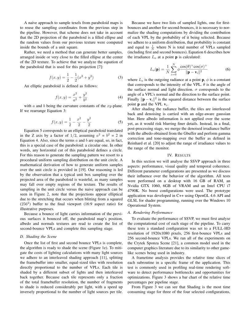
may fall over empty regions of the texture. The results of

sampling in the unit circle versus the naive approach can be

seen in Figure 2, note that the projections appear elliptical

due to the stretching that occurs when blitting from a squared

(2562) buffer to the final viewport (16:9 aspect ratio) for

illustrative purposes.

Because a bounce of light carries information of the previ-

ous surfaces it bounced off, the paraboloid map’s position,

albedo and normals textures are read to create the list of

second-bounce VPLs and complete this sampling stage.

D. Shading the Scene

Once the list of first and second bounce VPLs is complete,

the algorithm is ready to shade the scene (Figure 1e). To miti-

gate the costs of lighting calculations with many light sources

we adhere to an interleaved shading approach [11], splitting

the framebuffer into smaller, equal-sized tiles with resolution

directly proportional to the number of VPLs. Each tile is

shaded by a different subset of lights and then interleaved

back together. Because each tile represents only a fraction

of the total framebuffer resolution, the number of fragments

to shade is reduced considerably per light, with a speed up

inversely proportional to the number of light sources per tile.

Because we have two lists of sampled lights, one for first-

bounces and another for second-bounces, it is necessary to nor-

malize the shading computations by dividing the contribution

of each VPL by the probability of it being selected. Because

we adhere to a uniform distribution, that probability is constant

and equal to 1

Nwhere N is total number of VPLs sampled

(including first and second bounces). Equation 6 describes how

the irradiance Lo at a point p is calculated:

Lo(p) =1

N

N∑

i=0

φcos(θ)+cos(σ)+

‖p − vi‖2(6)

where Lo is the outgoing radiance at a point p, φ is a constant

that corresponds to the intensity of the VPL. θ is the angle of

the surface normal and light direction. σ corresponds to the

angle of a VPL’s normal and the direction to the surface point.

Finally ‖p − vi‖2 is the squared distance between the surface

point p and the VPL vi.

After shading the radiance buffer, the tiles are interleaved

back and denoising is carried with an edge-aware gaussian

blur. Here albedo information is not applied over the scene

yet, as it would risk blurring finer details. Instead, in a final,

post-processing stage, we merge the denoised irradiance buffer

with the albedo obtained from the Gbuffer and perform gamma

correction and tone-mapping over the buffer as defined in

Reinhard et al. [20] to adjust the range of irradiance values to

the range of the monitor.

IV. RESULTS

In this section we will analyse the SSVP approach in three

aspects: performance, visual quality and temporal coherence.

Different parameter configurations are presented as we discuss

their influence over the behavior of the algorithm. All tests

were performed on a desktop with 16 GB of RAM, an

Nvidia GTX 1060, 6GB of VRAM and an Intel CPU i7

4790K. No boost configurations were used. The prototype

application was developed in C++ using OpenGL 4.6 API and

GLSL for shader programming, running over the Windows 10

Operational System.

A. Rendering Performance

To evaluate the performance of SSVP, we must first analyse

the computational cost of each stage of the pipeline. To carry

these tests a standard configuration was set to a FULL-HD

resolution of 1920x1080 pixels, 256 first-bounce VPLs and

256 second-bounce VPLs. We ran all of the experiments on

the Crytek Sponza Scene [21], a common model used in the

computer graphics literature due to its similarity to other game-

like scenes being used in industry.

A frametime analysis provides the relative time slices of

each subroutine in a specific frame of the application. This

test is commonly used in profiling real-time rendering soft-

ware to detect performance bottlenecks and opportunities for

optimizations. Figure 3 shows a bar chart of the relative time

percentages per pipeline stage.

From Figure 3 we can see that Shading is the most time

consuming stage for three of the four selected configurations,

(a) Uniform Unit-Box Sampling (b) Uniform Unit-Disk Sampling

Fig. 2. 120 uniform samples (blue points) in (a) the unit box and (b) the unit disk. In (a), samples are spread over the space without taking the centralprojection in account. In (b), samples match the projected area in a more coherent pattern.

Fig. 3. Average time slices of our algorithm for the Crytek Sponza scene,running on a viewport with 1920x1080 resolution, 4x4 interleaved samplingpattern and multiple cluster configurations. Misc. includes the time to generatea shadow map, to sample first-bounce VPLs with the RSM, to cluster thoseVPLs, to sample second-bounce VPLs and to denoise the image.

but the trend decreases as the number of clusters grow. It’s

relative time slice of SSVP starts at 80% for 4 Clusters and

drops to 54% at 16 Clusters. With 32 Clusters, rendering

times become dominated by paraboloid rendering and total

frametime surpass the real-time threshold by a large amount.

Pixel processing operations impose relatively heavy loads over

the GPU compared to other tasks, therefore it is expected to

be the dominant stage with regard to time per stage of our

algorithm.

However, with more and more paraboloid maps requir-

ing computational resources to perform multiple rasterization

passes over the geometry, this stage quickly becomes a bot-

tleneck, surpassing shading as the most time consuming step

of SSVP. Notice the growth in time as we double the number

of paraboloid maps until we reach 16 clusters where a sudden

spike makes it grow considerably, then at 32 clusters the total

frametime is three times larger than the previous. From this

standpoint, analysis of the relative percentual cost reveals that

paraboloid creation can quickly become prohibitive for the

tight thresholds of real-time rendering. Table I provides the

total percentages and rendering times for each configuration.

Notice how for configurations of 4 and 8 clusters, the al-

gorithm was able to perform faster than the original 16ms

4 Clusters 8 Clusters 16 Clusters 32 Clusters

Gbuffer 1.03 1.03 1.03 1.03

Misc 0.26 0.29 0.30 0.30

Paraboloid 1.16 2.50 7.90 56.29

Shade 10.31 10.76 10.94 10.95

Denoise 0.13 0.14 0.14 0.18

Total(ms) 12.89 14.74 20.31 68.75TABLE I

RELATIVE TIME OF EACH SSVP PIPELINE STAGE AS THE NUMBER OF

CLUSTERS CHANGE. TIME IS GIVEN IN MILLISECONDS. MISC

CORRESPONDS TO THE TIME NEEDED TO GENERATE A SHADOW MAP, TO

SAMPLE FIRST-BOUNCE VPLS, TO CLUSTER THOSE VPLS AND TO

SAMPLE SECOND-BOUNCE VPLS AND TO DENOISE THE IMAGE.

threshold. for real time applications this would be the ideal

scenario.

On the other hand, the fastest stages in SSVP’s pipeline,

K-Means Clustering and VPL sampling account for no more

than 0.8% and 0.2% of a single frame for any configuration.

The reason behind these low percentages is that clustering here

is done on compute shaders to leverage GPU parallelism and

sampling is a trivial step that consists of reading texels from

paraboloids to create a second-bounce VPL list.

The time curve for different paraboloid configurations grows

in a seemingly linear fashion for 4, 8 and 16 Clusters, beyond

this point (at the change to 32) time appears to grow with

a steeper slope. Preliminary investigation of this behavior

implies in increasing cache misses and points synchronization

as we grow the number of render passes in geometry shaders,

but no experiments with different hardware configurations

were performed therefore a decisive evaluation can not be

provided here.

B. Visual Quality

To begin the visual quality tests we follow the trend in

the computer graphics literature of carrying a ground truth

comparison. The ground truth image was generated with the

industry standard Path-Tracing technique to render the same

Crytek Sponza model using the open source research-oriented

renderer Mitsuba [22], with 256 ray samples per pixel. Figure

4 presents a comparison between SSVP and the ground truth.

It shows the impact of allowing direct light to bounce two

times through the scene, and compare the final image to the

ground truth. The addition of second-bounce VPLs introduce

some effects such as color bleeding, seeing nearby the curtains

for example and make the shadows brighter, giving a proper

sense of indirect lighting.

Ideally we would like to render a visibility map for each

VPL in real-time, but as shown in Table I the cost of rendering

more paraboloids impact negatively in rendering performance.

For this reason, to align with the goals of SSVP, the practical

scenario requires a tradeoff between visual quality and per-

formance to favor real-time and game-like applications. To

this end, an evaluation of the visual impact of rendering more

clusters and more second-bounce VPLs in the final image is

carried. We focus on effects that stand out more easily to the

human eye, such as color bleeding and artifacts like banding.

Screenshots were taken during navigation of the scene

through the same path for 8, 16 and 32 clusters (Figure 5)

with 64, 256 and 1024 total second-bounce VPLs. Notice

the color bleeding effect nearby the pillars, colored lighting

bouncing off the curtains spreads through the floor and the

walls, painting them red, blue and green. In these images it

is also possible to notice artifacts known as light leaking, due

to the lack of precise visibility calculations sometimes light

spreads towards unwanted locations, making them brighter

than intended. Visually these effects are related mainly to the

number of second bounces being rendered, but for larger num-

bers of clusters more lights are required to achieve a similar

levels. Pay attention to Figure 5 how 256 second-bounce VPLs

provide clearer colors with 8 clusters in comparison to 16

and 32 clusters respectively. At 1024 VPLs all configurations

appear to converge achieving similar results. No further effects

arise from higher configurations, but light leaking becomes

easier to notice.

A promptly noticeable effect of rendering with reduced

cluster count is the amount of banding artifacts on the edges of

shadows for single bounce lighting (shadows on the walls and

in the back of the scene). As more visibility maps are included,

these artifacts tend to soften and for very large numbers of

visibility maps (hundreds of thousands [3]) they converge

into soft-shadows. However, notice how adding second-bounce

VPLs provides a huge benefit in this case, hiding these artifacts

by spreading more light over the surfaces and attenuating the

banding. This reasoning guides the evaluation in this stage,

the fastest possible configuration that still maintains visual

plausibility is the one that better fits the objective of SSVP.

Going further in Figure 6 we compare different cluster

configurations over the scene using the HDR-VDP-2 metric

[23] to evaluate the error between an image and a reference.

The scene rendered with the most clusters (32) is used as the

baseline and the perceptual error metric is calculated for 16,

8 and 4 clusters.

The root-mean-square error computed for 4 clusters (Figure

6e) is 0.1888, 8 clusters (Figure 6f) is 0.1111 and 16 clusters

(Figure 6g) is 0.0936. The higher this value the more likely an

observer is to perceive differences in comparison to the refer-

ence image. The results from the second-bounce comparison

and HDR-VDP-2 imply that 16 clusters offers superior quality

over lesser configurations.

C. Temporal Coherence

The temporal coherence of a method evaluates how stable

a rendering algorithm performs for animated scenes, with

moving cameras or light sources.

To better analyse the coherence of SSVP we point the reader

to the videos in the supplemental material. This analysis is

complex and deserves a research of its own as can be seen over

the literature [24]. However SSVP introduces some techniques

to alleviate the impact of flickering when navigating the scene

by reusing cluster positions between frames and repeating the

sampling patterns. Because of this, SSVP is stable when mov-

ing the camera around the scene while keeping the directional

light source static. However, with dynamic light sources, a few

visual artifacts can be seen as in the black stripe over the red

curtain in Figure 7, mainly as a byproduct of cluster visibility

changing due to centroids moving along surfaces.

V. DISCUSSION

Starting from the definition that 60 frames per second (16

milliseconds per frame) is the optimal frame rate for hard real-

time applications, illumination algorithms must be computed at

frame times lower than that threshold, as such applications still

need time to compute other tasks such as in-game logic and

physics updates. The data in Table I shows that SSVP is able

to offer the speed needed for such highly interactive game-like

scenarios with average frame rates of 13 milliseconds for the

compromise configuration provided. The cost of performing

the lighting computations is mitigated here by interleaved

sampling, but this stage is expected to become slower as the

number of pixels grow, therefore a 1080p FULL-HD resolution

is recommended to favor performance. SSVP’s visual quality

is deeply reliant on the number of clusters we use to compute

visibility. However, increasing the number of paraboloid maps

too much will beat the purpose of the technique and imply

a heavy toll over frame rate. For this reason we would like

to render the minimum amount of paraboloid shadow maps

that preserves the plausibility of the visuals. The results from

the second-bounce comparison and HDR-VDP-2 combined are

aligned with our empirical evaluation, leading us to conclude

that 8 clusters suffice to preserve visual plausibility with render

times within the stabilished threshold of 16 milliseconds.

To enable typically aesthetically pleasing effects such as

color bleeding at least 256 second-bounce VPLs are needed for

any cluster configuration in the scene tested. Visual perception

metrics (HDR-VDP-2) suggest that for the Sponza scene, 8

clusters are enough to plausibly emulate indirect lighting at

rates lower than 16 milliseconds. An obvious drawback of

our approach is that we are unable to reproduce soft shadows

and self-occlusion natively, therefore it is mandatory to resort

to orthogonal methods for such effects. Finally, the visual

quality of SSVP is directly tied to the number of clusters

and second-bounces generated, for this reason increasing first-

bounce count will offer no further benefits over quality because

of the lack of visibility computations for every new VPL that is

introduced. In our experiments 256 first-bounce VPLs proved

good enough for our measurements of cluster stability but

(a) SSVP (One Bounce) (b) SSVP (Two Bounces) (c) Path-Tracing (Ground Truth)

Fig. 4. Difference between one (a) and two (b) bounces of light rendered by our technique when compared to the ground-truth (c).

(a) 8 clusters (64 2nd-Bounces) (b) 8 clusters (256 2nd-Bounces) (c) 8 clusters (1024 2nd-Bounces)

(d) 16 clusters (64 2nd-Bounces) (e) 16 clusters (256 2nd-Bounces) (f) 16 clusters (1024 2nd-Bounces)

(g) 32 clusters (64 2nd-Bounces) (h) 32 clusters (256 2nd-Bounces) (i) 32 clusters (1024 2nd-Bounces)

Fig. 5. Sponza rendered from the same viewpoint for different cluster configurations. To compute the number of second bounce VPLs sampled per clusters,divide the total number of VPLs by the number of clusters.

since our method allows for custom parametrization, the reader

is encouraged to experiment given custom needs.

VI. CONCLUSION AND FUTURE WORKS

With SSVP we extended VPL clusterization techniques to

reproduce diffuse indirect illumination for up to two diffuse

bounces of light under real-time requirements. Given the hard

requirements for global illumination in game-like scenarios,

we obtained at a method that could represent plausible images

under the required time constraints with temporal coherence

for moving cameras and reasonable results for dynamic lights.

Furthermore, despite mitigating the costs of shading with many

light sources, interleaved shading introduces structured noise

in the final image. Since removing these prove to be more

difficult than typical pseudorandom white-noise, we believe

new approaches to shading with many lights could be explored

following the research of [25] with monte-carlo methods

for VPL selection and distributing noise in a more visually

pleasant manner.

ACKNOWLEDGMENT

Marcio C. F. Macedo is financially supported by the

Postdoctoral National Program of the Coordination for the

Improvement of Higher Education Personnel (PNPD/CAPES),

grant number 88882.306277/2018-01. The authors would also

like to thank the National Council for Scientific and Techno-

logical Development for the financial support.

REFERENCES

[1] J. T. Kajiya, “The rendering equation,” in Proceedings of SIGGRAPH.ACM, 1986, pp. 143–150.

[2] H. W. Jensen, “Global illumination using photon maps,” in Rendering

Techniques’ 96. Springer, 1996, pp. 21–30.

(a) (b) (c) (d)

(e) (f) (g)

Fig. 6. HDR-VDP-2 metric applied to images generated with 4, 8 and 16 clusters (Figures 6a, 6b and 6c respectively) in comparison to 32 clusters in Figure6d. Figures 6e, 6f and 6g show the perceptual error metric for 4, 8 and 16 clusters when compared to the base image with 32 clusters.

(a) (b)

Fig. 7. The visibility map of a moving centroid changes with time with dynamic light sources, potentially causing temporally incoherent visual artifacts ascan be seen on the red curtain and the light blotch nearby the blue curtain on the right.

[3] A. Keller, “Instant Radiosity,” in Proceedings of the SIGGRAPH. ACM,1997, pp. 49–56.

[4] T. Ritschel, T. Grosch, M. H. Kim, H.-P. Seidel, C. Dachsbacher, andJ. Kautz, “Imperfect shadow maps for efficient computation of indirectillumination,” in ACM Transactions on Graphics (TOG), vol. 27, no. 5.ACM, 2008, p. 129.

[5] M. McGuire and M. Mara, “Efficient gpu screen-space ray tracing,”Journal of Computer Graphics Techniques (JCGT), vol. 3, no. 4, pp.73–85, 2014.

[6] T. Ritschel, T. Grosch, and H.-P. Seidel, “Approximating dynamic globalillumination in image space,” in Proceedings of the I3D. ACM, 2009,pp. 75–82.

[7] W. Heidrich and H.-P. Seidel, “View-independent Environment Maps.”in Workshop on Graphics Hardware, 1998, pp. 39–45.

[8] C. Dachsbacher and M. Stamminger, “Reflective shadow maps,” inProceedings of the I3D. ACM, 2005, pp. 203–231.

[9] C. Dachsbacher, J. Krivanek, M. Hasan, A. Arbree, B. Walter, andJ. Novak, “Scalable realistic rendering with many-light methods,” inComputer Graphics Forum, vol. 33, no. 1. Wiley Online Library, 2014,pp. 88–104.

[10] C. Dachsbacher and M. Stamminger, “Splatting indirect illumination,”in Proceedings of the I3D. ACM, 2006, pp. 93–100.

[11] B. Segovia, J. C. Iehl, R. Mitanchey, and B. Peroche, “Non-interleaveddeferred shading of interleaved sample patterns,” in Graphics Hardware,2006, pp. 53–60.

[12] M. Hasan, J. Krivanek, B. Walter, and K. Bala, “Virtual spherical lightsfor many-light rendering of glossy scenes,” in ACM Transactions on

graphics (TOG), vol. 28, no. 5. ACM, 2009, p. 143.[13] Z. Dong, T. Grosch, T. Ritschel, J. Kautz, and H.-P. Seidel, “Real-time

Indirect Illumination with Clustered Visibility,” in Proceedings of the

VMV, vol. 9, 2009, pp. 187–196.[14] Y. Tokuyoshi, “Virtual Spherical Gaussian Lights for Real-time Glossy

Indirect Illumination,” in Computer Graphics Forum, vol. 34, no. 7.Wiley Online Library, 2015, pp. 89–98.

[15] P. Hedman, T. Karras, and J. Lehtinen, “Sequential monte carlo instantradiosity,” in Proceedings of the I3D. ACM, 2016, pp. 121–128.

[16] M. Mara, M. McGuire, D. Nowrouzezahrai, and D. P. Luebke, “Deepg-buffers for stable global illumination approximation.” in High Perfor-

mance Graphics, 2016, pp. 87–98.[17] M. Deering, S. Winner, B. Schediwy, C. Duffy, and N. Hunt, “The

triangle processor and normal vector shader: a vlsi system for highperformance graphics,” in Proceedings of the SIGGRAPH, vol. 22, no. 4.ACM, 1988, pp. 21–30.

[18] T.-T. Wong, W.-S. Luk, and P.-A. Heng, “Sampling with hammersleyand halton points,” Journal of graphics tools, vol. 2, no. 2, pp. 9–24,1997.

[19] M. Pharr, W. Jakob, and G. Humphreys, Physically based rendering:

From theory to implementation. Morgan Kaufmann, 2016.[20] E. Reinhard, M. Stark, P. Shirley, and J. Ferwerda, “Photographic tone

reproduction for digital images,” in Proceedings of the 29th annual

conference on Computer graphics and interactive techniques, 2002, pp.267–276.

[21] M. McGuire, “Computer Graphics Archive,” July 2017. [Online].Available: https://casual-effects.com/data

[22] W. Jakob, “Mitsuba renderer,” 2010, http://www.mitsuba-renderer.org.[23] R. Mantiuk, K. J. Kim, A. G. Rempel, and W. Heidrich, “Hdr-vdp-2:

A calibrated visual metric for visibility and quality predictions in allluminance conditions,” ACM Transactions on graphics (TOG), vol. 30,no. 4, pp. 1–14, 2011.

[24] D. Scherzer, L. Yang, O. Mattausch, D. Nehab, P. V. Sander, M. Wim-mer, and E. Eisemann, “Temporal coherence methods in real-timerendering,” in Computer Graphics Forum, vol. 31, no. 8. Wiley OnlineLibrary, 2012, pp. 2378–2408.

[25] E. Heitz and L. Belcour, “Distributing monte carlo errors as a blue noisein screen space by permuting pixel seeds between frames,” in Computer

Graphics Forum, vol. 38, no. 4. Wiley Online Library, 2019, pp. 149–158.