Embed Size (px)
Citation preview

Screened PoissonSurface Reconstruction
Misha KazhdanJohns Hopkins University
Hugues HoppeMicrosoft Research

Motivation3D scanners are everywhere:• Time of flight• Structured light• Stereo images• Shape from shading• Etc.
http://graphics.stanford.edu/projects/mich/

Geometryprocessing
Motivation
Parameterization
Decimation
Filtering
etc.
Surfacereconstruction

Implicit Function FittingGiven point samples:– Define a function with value zero at the points.– Extract the zero isosurface. >0
<0
0
F(q)Sample points
F(q)<0
F(q)>0
F(q) =0

Related work
[Kazhdan et al. 2006]
[Hoppe et al. 1992] [Curless and Levoy 1996]
[Calakli and Taubin 2011][Alliez et al. 2007]
[Carr et al. 2001]
… and many more …

Poisson Surface Reconstruction [2006]– Oriented points samples of indicator gradient.– Fit a scalar field to the gradients.
∇ 𝜒=𝑉
𝜒 (𝑞) 𝑉 (𝑞 )
𝜒=min𝐹
‖∇𝐹−𝑉‖2
(q)=-0.5
(q)=0.5
Poisson Surface Reconstruction [2006]1. Compute the divergence2. Solve the Poisson equation
𝑉 (𝑞 )
∇⋅ Δ−1
𝜒 (𝑞)

Poisson Surface Reconstruction [2006]1. Compute the divergence2. Solve the Poisson equation
Discretize over an octree Update coarse fine
coarse
fine
+
+
+
+
Solution Correction
𝑉 (𝑞 )
Δ−1
𝜒 (𝑞)
∇⋅

Poisson Surface Reconstruction [2006]
Properties: Supports noisy, non-uniform data Over-smoothes Solver time is super-linear

Screened Poisson Reconstruction• Higher fidelity – at same triangle count• Faster – solver time is linear
Screened PoissonPoisson

Outline• Introduction
• Better / faster reconstruction
• Evaluation
• Conclusion

Better ReconstructionAdd discrete interpolation to the energy:
– encouraged to be zero at samples
Adds a bilinear SPD term to the energy Introduces inhomogeneity into the system
𝐸 ( 𝜒 )=∫‖∇ 𝜒 (𝑞)−𝑉 (𝑞)‖2ⅆ𝑞 Gradient fitting Sample interpolation
[Carr et al.,…,Calakli and Taubin]
+𝜆∑𝑝∈𝑃
‖𝜒 (𝑝 )−0‖2

Better ReconstructionDiscretization:Choose basis to represent :
𝜒 (𝑞)=∑𝑖=1
𝑛
𝑥𝑖𝐵𝑖 (𝑞 )
𝐵𝑖− 1 (𝑞 ) 𝐵𝑖 (𝑞) 𝐵𝑖+1 (𝑞 ) 𝐵𝑖+2 (𝑞 )
𝑥𝑖 −1
𝑥𝑖
𝑥𝑖+1
𝑥𝑖+2

Better ReconstructionDiscretization:For an octree, use B-splines:– centered on each node– scaled to the node size

Better ReconstructionPoisson reconstruction:To compute , solve:
with coefficients given by:
Screened
^
𝐿𝑥=𝑏
𝑏𝑖=∫ ⟨∇𝐵𝑖 (𝑞 ) ,𝑉 (𝑞 ) ⟩ ⅆ𝑞𝐿𝑖𝑗=∫ ⟨∇𝐵 𝑖 (𝑞 ) ,∇𝐵 𝑗 (𝑞 ) ⟩ⅆ𝑞+𝜆∑
𝑝∈𝑃
𝐵𝑖 (𝑝 )𝐵 𝑗 (𝑝)Bi
Bj

Poisson reconstruction:Sparsity is unchangedEntries are data-dependent
Better Reconstruction
𝑏𝑖=∫ ⟨∇𝐵𝑖 (𝑞 ) ,𝑉 (𝑞 ) ⟩ ⅆ𝑞
Screened
^
𝐿𝑖𝑗=∫ ⟨∇𝐵 𝑖 (𝑞 ) ,∇𝐵 𝑗 (𝑞 ) ⟩ⅆ𝑞+𝜆∑𝑝∈𝑃
𝐵𝑖 (𝑝 )𝐵 𝑗 (𝑝)Bi
Bj
Bj
Bi

Faster Screened ReconstructionObservation:At coarse resolutions, no need to screen as precisely. Use average position,
weighted by point count.Bj
Bi BjBi
BjBi

Faster ReconstructionSolver inefficiency:Before updating, subtract constraints met at all coarser levels of the octree. complexity
coarse
fine
+
+
+
Solution Correction
𝜒 (𝑞)

Faster Reconstruction
Regular multigrid:Function spaces nest can upsample coarser
solutions to finer levels

Faster Reconstruction
Adaptive multigrid: Function spaces do not nest coarser solutions need to
be stored explicitly

Faster Reconstruction
Naive enrichment: Complete octree
Faster Reconstruction
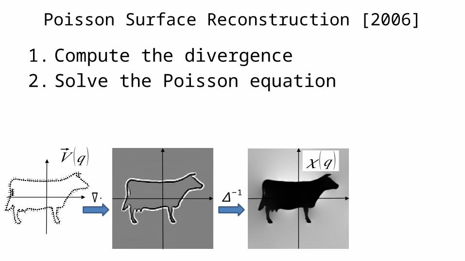
Observation:Only upsample the part ofthe solution visible to the finer basis.

Faster Reconstruction
Enrichment:Iterate fine coarse
Identify support of next-finer levelAdd visible functions

Faster Reconstruction
Original Enriched

Faster Reconstruction
Adaptive Poisson solver: Update coarse fine
Get supported solution
Adjust constraints
Solve residual
+
+
+
+
+
+
+
+
+
+
+
Solution Correction Visible Solution
𝜒 (𝑞)

Outline• Introduction
• Better / faster reconstruction
• Evaluation
• Conclusion

AccuracyPoisson Screened Poisson
𝑥
𝑧 z
𝑥
SSD [Calakli & Taubin]
z
𝑥
𝑧 𝑧

AccuracyPoisson Screened Poisson SSD [Calakli & Taubin]
𝑥
𝑧
𝑥
𝑧
𝑥
𝑧

Performance
Input: 2x10⁶ points
Solver Time Space
Poisson 89 sec 422 MB
Poisson (optimized) 36 sec604 MB
Screened Poisson 44 sec
SSD [Calakli & Taubin] 3302 sec 1247 MB

Input: 5x10⁶ points
Performance
Solver Time Space
Poisson 412 sec 1498 MB
Poisson (optimized) 149 sec2194 MB
Screened Poisson 172 sec
SSD [Calakli & Taubin] 19,158 sec 4895 MB
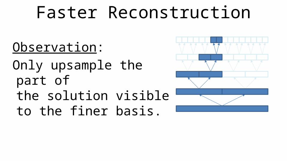
Limitations Assumes clean data
Poisson Screened Poisson
𝑥
𝑧
Summary
Screened Poisson reconstruction:
Sharper reconstructions
Optimal-complexity solver

Future Work• Robust handling of noise• (Non-watertight reconstruction)• Extension to full multigrid

Data:Aim@Shape, Digne et al., EPFL,Stanford Shape Repository
Code:Berger et al., Calakli et al.,Manson et al.
Funding:NSF Career Grant (#6801727)
Thank You!
http://www.cs.jhu.edu/~misha/Code/PoissonRecon