Scripting in high performance computing environment

RESEARCH REPORT VTT-R-03683-15

SIMPRO Scripting in high performance computing environment Authors: Kai Katajamäki

Confidentiality: Public (starting from August 31, 2015)


1 (21)

Report’s title

Scripting in high performance computing environment Customer, contact person, address Order reference

Tekes, Matti Säynätjoki P.O. Box 69, FI-00101 Helsinki, Finland

1059/31/2012

Project name Project number/Short name

Computational methods in mechanical engineering product development

78634/SIMPRO

Author(s) Pages

Kai Katajamäki 21 Keywords Report identification code

scripting, python VTT-R-03683-15 Summary Effective use of high performance computing environment requires knowledge and know-how of scripting languages. With scripting the user can automate and develop users own routines which can speed-up the modelling and analysis time enormously. Also, scripting enables in-tegration between different software in an effective way. In product design the need of seam-less integration of optimization and structural and other analysis software can be fulfilled with relatively easy using some scripting language. One of the most popular scripting languages is Python. It is a modern programming language, which has become popular in many applica-tion areas. It is easy to learn and use in basic programming tasks but especially many sepa-rate modules widen its application areas and usability remarkably. For example for large scale scientific calculations the NumPy module enables effective calculations due to its spe-cial array class. Python is also an object-oriented language thus making possible the use of classes and objects. This is a background study in scripting in high performance computing environment. The fo-cus is on the Python language. In this work the basic functionality and syntax is presented. Also some library packages are described. Information on the documentation and tutorials as well as integrated development environments is given. Example scripts to demonstrate the basic use of the language and external modules are also given.

Confidentiality Public (starting from August 31, 2015) Espoo 13.8.2015 Written by Kai Katajamäki Principal Scientist

Reviewed by Aku Karvinen Senior Scientist

Accepted by Johannes Hyrynen Head of Research Area

VTT’s contact address VTT Technical Research Centre of Finland Ltd, P.O. Box 1000, FI-02044 VTT, Finland Distribution (customer and VTT) Matti Säynätjoki, Tekes, 1 copy VTT, 1 copy

The use of the name of VTT Technical Research Centre of Finland Ltd in advertising or publishing of a part of this report is only permissible with written authorisation from VTT Technical Research Centre of Finland Ltd.


2 (21)

Contents

Contents ................................................................................................................................. 2

1. Introduction ....................................................................................................................... 3

2. Scripting with Python ........................................................................................................ 3

2.1 Basic commands ...................................................................................................... 4 2.2 Python versions ........................................................................................................ 8 2.3 Development environments ...................................................................................... 9

3. Scripting in modelling and simulation process ................................................................. 10

3.1 NumPy module ....................................................................................................... 10 3.2 Matplotlib plotting library ......................................................................................... 12 3.3 Python scripting in visualization .............................................................................. 14

4. Conclusions .................................................................................................................... 16


3 (21)

1. Introduction

Effective use of high performance computing environment requires knowledge and know-how of scripting languages. With scripting the user can automate and develop users own routines which can speed-up the modelling and analysis time enormously. Also, scripting enables integration between different software in an effective way. In product design the need of seamless integration of optimization and structural and other analysis software can be fulfilled with relatively easy using some scripting language. One of the most popular scripting languages is Python (https://www.python.org/). Python is a modern programming language and it has become popular in many application areas. There are special libraries which widen the basic programming possibilities with whole new features. For example for scientific computing there is NumPy (http://www.numpy.org/) module. It is an extension to Python which adds support for large, multi-dimensional arrays and matrices. Also many mathematical functions to operate these arrays are available in this extension. For plotting purposes there is Matplotlib extension (http://matplotlib.org/). SciPy (http://www.scipy.org/) is a wide package aimed at scientific and engineering problems. It has its own library for scien-tific computing and it also includes NumPy and Matplotlib packages.

Some modelling, simulation and visualization software has chosen Python as its scripting language. For example widely used commercial structural analysis software Abaqus (http://www.3ds.com/products-services/simulia/portfolio/abaqus/overview/) as well as non-commercial finite element software Code_Aster (http://www.code-aster.org/) uses it. Python is integrated also in the general pre- and post-processing software Salome (http://www.salome-platform.org/). Another analysis software example is the simulation framework Yade (https://yade-dem.org/doc/) which is focused on Discrete Element Method. It uses Python for model preparation and controlling the simulations and simulation results. ParaView (http://www.paraview.org/) is software aimed at large-scale scientific visualization. The data exploration can be done programmatically using its batch processing capabilities which take advantage of the Python language. The above list is only a small portion of the wide range of applications where Python is used.

In this work basic programming with Python is presented. Some of the basic commands and programming syntax are described. Some notes on tutorials, development environments and running the Python interpreter are given. As an example of Python library usage, NumPy and Matplotlib libraries are used. Simple example scripts are listed and described. Some simple examples are also given how Python scripting language can run visualization software.

2. Scripting with Python

Python is a powerful programming language which has become a popular tool in scientific computing. Because it is an interpreted language, the time required to start programming with it is short. In its simplest usage mode one only needs to launch an interactive shell and start giving Python commands in it. The commands are then interpreted directly in the shell.

Although Python is easy to learn and use it is still a full-featured object oriented programming language having all the features that enable handling wide range of needs. A good starting point in learning to program and use Python language is the rich information which can be found on the Python community home pages. Basic information for those Python learners who do not have any or have only very little previous programming experience can be found at https://wiki.python.org/moin/BeginnersGuide/NonProgrammers. For those who have al-ready experience with some other programming languages similar learning information is located at https://wiki.python.org/moin/BeginnersGuide/Programmers.

Python is under an open source license thus making it freely usable and distributable. This applies to as well academic as pure commercial use. Moreover, it is available for all major

https://www.python.org/

http://www.numpy.org/

http://matplotlib.org/

http://www.scipy.org/

http://www.3ds.com/products-services/simulia/portfolio/abaqus/overview/

http://www.code-aster.org/

http://www.salome-platform.org/

https://yade-dem.org/doc/

http://www.paraview.org/

https://wiki.python.org/moin/BeginnersGuide/NonProgrammers

https://wiki.python.org/moin/BeginnersGuide/Programmers


4 (21)

operating systems, for example Windows, Linux and Mac OS X. The same source code will run unchanged under different systems which is a big advantage in software development.

2.1 Basic commands

Below is described with examples some basic but nevertheless important features of Python programming language. The used syntax of the examples is according to Python version 2. It should be mentioned that the newer Python version 3 has somewhat different syntax. Be-cause version 2 is still far more popular the focus is in this report on the older program ver-sion.

• Python 2 supports following variable types

o int ─ integers o long ─ long integers o float ─ floating point numbers o complex ─ complex numbers o str ─ strings. Python strings are a set of characters en-

closed in quotation marks. Python allows either single or double quotes.

• Variable names are case sensitive, for example World is different from WORLD

• No type declaration is needed meaning that variables are directly affected with the equal sign

>>> a = 10.1 >>> b = 8. * a – 5.

• Integers are treated as pure integers in mathematical operations. One should be careful when dealing with integers: 1/2 returns 0 whereas 1./2 returns 0.5. In Py-thon version 3 the division of two integers results in a floating point number. If one wants to have Python 2 to have similar integer division then he can give __future__ -statement

>>> from __future__ import division

• Complex numbers are given as:

>>> z = 1 + 2j,

real part is obtained with

>>> z.real

and imaginary part with

>>> z.imag

• Simple conversions for number to text and text to number:

>>> str(9) >>> int(‘123’) >>> float(‘3.14’)

• Basic arithmetic operations are available: +, -, *, /, **. As in the integer division also other arithmetic operations on integer values result in an integer number. Thus for example the exponentiation

>>> 8 ** 3 produces 512 while >>> 8.0 ** 3 produces 512.0.

It should also be noted that the operator ^ which is common in many other program-ming languages, is a bitwise XOR operator in Python. Consequently in Python

>>> 8 ^ 3 produces 11 and


5 (21)

>>> 3 ^ 8 produces as well 11.

The operator ^ treats two numbers, x and y, in their binary presentations (so called two’s complement) and it does a bitwise exclusive or comparison (XOR) between them, written in general as x ^ y. Each bit of the output is the same as the corre-sponding bit in x if that bit in y is 0, and it’s the complement of the bit in x if that bit in y is 1. In the example above x has a value of 8. Then its binary presentation is 1000 (1 × 23 + 0 × 22 + 0 × 21 + 0 × 20). y has a value of 3 and its binary presentation is then 0011 (0 × 23 + 0 × 22 + 1 × 21 + 1 × 20). The bitwise XOR comparison gives as a result the binary system number 1011. This value in decimal number system is 11 (1 × 23 + 0 × 22 + 1 × 21 + 1 × 20).

• Comments in Python start with the hash mark, #, and extend to the end of the physi-

cal line.

>>> # this is a comment

One gains access to a special module of functions by importing the modules. Below is an example how to import the math module and how to use it.

>>> import math >>> a = math.sqrt(2) >>> import math as m # use the module under a different name >>> b = m.cos(m.pi) >>> from math import * # import everything, functions can then be

# used directly without giving the module # name

>>> c = cos(pi)

• Code blocks are indicated by indentation. This rule is mandatory to follow.

>>> i = 0 >>> while i < 10: … print i … i = i + 1 … >>> print ‘end’

• String concatenation is easy:

>>> text1 = ‘hello’ >>> text2 = ‘ world’ >>> text3 = text1 + text2 # this produces string ‘hello world’

Building long strings using this method can result in very slow running code. In Py-thon a string object is immutable i.e. each time a string is assigned to a variable a new object is created in memory. There are more effective ways to handle strings. One can use list comprehensions and then the above example can be written to pro-duce more effective code as:

>>> str_list=[] >>> str_list.append(text1) >>> str_list.append(tex2) >>> text3 = ’’.join(str_list)

The last line uses the join() method of the String class. The method joins the strings given in str_list into given string. In this case the latter is an empty string given as two single quotes. The above code can be programmed more compactly:


6 (21)

>>> text3 = ’’.join([text1, text2]) # this produces ‘hello world’ >>> text3 = ’-’.join([text1, text2]) # this produces ‘hello- world’

• Control structures

If…elif…else statement >>> if x == 1: … print ‘A’ … elif x == ‘hello’ or y <= 1: … z = z + 1 … else: … w = w**4

While loop >>> while a < b: … a +=1 … print a

For loop >>> for i in range(5): … print i # Note: in this example the integer variable i gets values 0,1,2,3,4

Brake statement >>> for let in ‘World’: … if let == ‘l’: … break … print let >>> # Brake statement terminates the loop and resumes execution at >>> # the next statemen after the loop.

Continue statement >>> for let in ‘World’: … if let == ‘l’: … continue … print let >>> # Continue statement rejects all the remaining statements in the >>> # current iteration and returns the control to the beginning of >>> # the loop. It can be used in for and while loops.

• A Python list consists of items separated by commas and enclosed within square brackets. A list can include different data types and even other lists. Note that the in-dex of the first item in a list is always 0, for example my_list[0].

List creation

>>> a = [4, 7, ‘text’, 3.14] >>> b = [3, -2+3j, [8, 9], ‘asd’]

List concatenation

>>> a + b → [4, 7, ‘text’, 3.14, 3, -2+3j, [8, 9], ‘asd’]

Appending an item to a list

>>> a.append(‘newitem’) → [4, 7, ‘text’, 3.14, ‘newitem’]

Length of the list

>>> len(b) → 4 >>> len(b[2]) → 2

Item manipulation


7 (21)

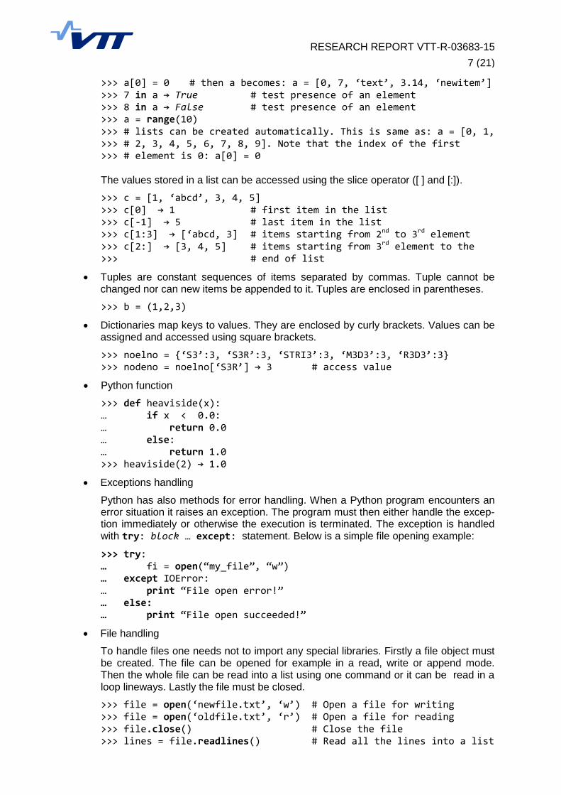
>>> a[0] = 0 # then a becomes: a = [0, 7, ‘text’, 3.14, ‘newitem’] >>> 7 in a → True # test presence of an element >>> 8 in a → False # test presence of an element >>> a = range(10) >>> # lists can be created automatically. This is same as: a = [0, 1, >>> # 2, 3, 4, 5, 6, 7, 8, 9]. Note that the index of the first >>> # element is 0: a[0] = 0 The values stored in a list can be accessed using the slice operator ([ ] and [:]).

>>> c = [1, ‘abcd’, 3, 4, 5] >>> c[0] → 1 # first item in the list >>> c[-1] → 5 # last item in the list >>> c[1:3] → [‘abcd, 3] # items starting from 2nd to 3rd element >>> c[2:] → [3, 4, 5] # items starting from 3rd element to the >>> # end of list

• Tuples are constant sequences of items separated by commas. Tuple cannot be changed nor can new items be appended to it. Tuples are enclosed in parentheses.

>>> b = (1,2,3)

• Dictionaries map keys to values. They are enclosed by curly brackets. Values can be assigned and accessed using square brackets.

>>> noelno = {‘S3’:3, ‘S3R’:3, ‘STRI3’:3, ‘M3D3’:3, ‘R3D3’:3} >>> nodeno = noelno[‘S3R’] → 3 # access value

• Python function

>>> def heaviside(x): … if x < 0.0: … return 0.0 … else: … return 1.0 >>> heaviside(2) → 1.0

• Exceptions handling

Python has also methods for error handling. When a Python program encounters an error situation it raises an exception. The program must then either handle the excep-tion immediately or otherwise the execution is terminated. The exception is handled with try: block … except: statement. Below is a simple file opening example:

>>> try: … fi = open(“my_file”, “w”) … except IOError: … print “File open error!” … else: … print “File open succeeded!”

• File handling

To handle files one needs not to import any special libraries. Firstly a file object must be created. The file can be opened for example in a read, write or append mode. Then the whole file can be read into a list using one command or it can be read in a loop lineways. Lastly the file must be closed.

>>> file = open(‘newfile.txt’, ‘w’) # Open a file for writing >>> file = open(‘oldfile.txt’, ‘r’) # Open a file for reading >>> file.close() # Close the file >>> lines = file.readlines() # Read all the lines into a list


8 (21)

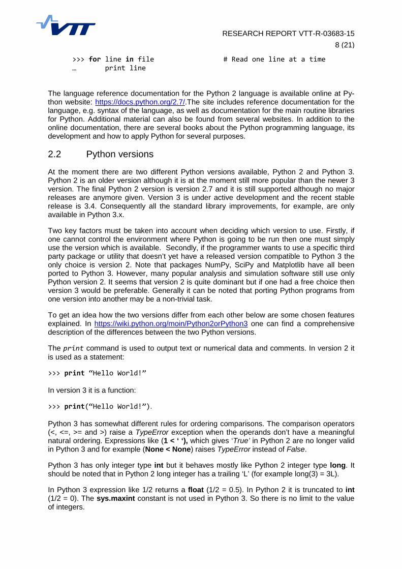
>>> for line in file # Read one line at a time … print line

The language reference documentation for the Python 2 language is available online at Py-thon website: https://docs.python.org/2.7/.The site includes reference documentation for the language, e.g. syntax of the language, as well as documentation for the main routine libraries for Python. Additional material can also be found from several websites. In addition to the online documentation, there are several books about the Python programming language, its development and how to apply Python for several purposes.

2.2 Python versions

At the moment there are two different Python versions available, Python 2 and Python 3. Python 2 is an older version although it is at the moment still more popular than the newer 3 version. The final Python 2 version is version 2.7 and it is still supported although no major releases are anymore given. Version 3 is under active development and the recent stable release is 3.4. Consequently all the standard library improvements, for example, are only available in Python 3.x.

Two key factors must be taken into account when deciding which version to use. Firstly, if one cannot control the environment where Python is going to be run then one must simply use the version which is available. Secondly, if the programmer wants to use a specific third party package or utility that doesn’t yet have a released version compatible to Python 3 the only choice is version 2. Note that packages NumPy, SciPy and Matplotlib have all been ported to Python 3. However, many popular analysis and simulation software still use only Python version 2. It seems that version 2 is quite dominant but if one had a free choice then version 3 would be preferable. Generally it can be noted that porting Python programs from one version into another may be a non-trivial task.

To get an idea how the two versions differ from each other below are some chosen features explained. In https://wiki.python.org/moin/Python2orPython3 one can find a comprehensive description of the differences between the two Python versions.

The print command is used to output text or numerical data and comments. In version 2 it is used as a statement:

>>> print “Hello World!” In version 3 it is a function:

>>> print(“Hello World!”). Python 3 has somewhat different rules for ordering comparisons. The comparison operators (<, <=, >= and >) raise a TypeError exception when the operands don’t have a meaningful natural ordering. Expressions like (1 < ‘ ‘), which gives ‘True’ in Python 2 are no longer valid in Python 3 and for example (None < None) raises TypeError instead of False.

Python 3 has only integer type int but it behaves mostly like Python 2 integer type long. It should be noted that in Python 2 long integer has a trailing ‘L’ (for example long(3) = 3L).

In Python 3 expression like 1/2 returns a float (1/2 = 0.5). In Python 2 it is truncated to int (1/2 = 0). The sys.maxint constant is not used in Python 3. So there is no limit to the value of integers.

https://docs.python.org/2.7/

https://wiki.python.org/moin/Python2orPython3


9 (21)

In order to port source code written in Python 2 into version 3 there is a Python program called 2to3 (https://docs.python.org/2/library/2to3.html). It reads Python 2 source code and applies a series of fixers to transform it into Python 3 code.

2.3 Development environments

Since Python is an interpreted language, the scripts can be prepared simply by using some text editing program. The files can then be directly run in a terminal window without the need to compile and link the source and object code to get an executable. For more demanding programming needs it is however desirable to have some kind of software development envi-ronment. The Python installation usually includes IDLE (Integrated DeveLopment Environ-ment) provided that the platform supports Tcl. It is a cross-platform environment thus running on Windows and Unix/Linux.

Another development environment is PyDev which is a Python IDE for Eclipse. Its internet site is located at http://pydev.org/ where one finds installation instructions and a getting start-ed manual.

In general there are many Python IDEs available. A comprehensive list can be found at the Python website: http://wiki.python.org/moin/IntegratedDevelopmentEnvironments. The site lists the following IDEs and much more:

• Komodo • NetBeans • PyCharm • PyDev • PyScripter • Pyshield • Spyder • IDLE • IdleX • µ.dev • IEP • PythonToolkit (PTK) • PyStudio • Python Tools for Visual Studio

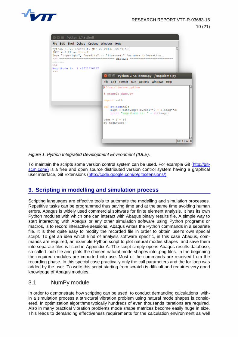
Figure 1 shows the windows of Python IDLE. It has two main windows, namely the Shell window and the Editor window. It is possible to have multiple editor windows simultane-ously open. The editor window has syntax highlighting and many editing tools including function parameter hints. The scripts can be run directly from the editor window and there is also program code debugging feature. Documentation on the IDLE can be found at the Python website https://docs.python.org/2/library/idle.html.

https://docs.python.org/2/library/2to3.html

http://pydev.org/

http://wiki.python.org/moin/IntegratedDevelopmentEnvironments

https://docs.python.org/2/library/idle.html


10 (21)

Figure 1. Python Integrated Development Environment (IDLE).

To maintain the scripts some version control system can be used. For example Git (http://git-scm.com/) is a free and open source distributed version control system having a graphical user interface, Git Extensions (http://code.google.com/p/gitextensions/).

3. Scripting in modelling and simulation process

Scripting languages are effective tools to automate the modelling and simulation processes. Repetitive tasks can be programmed thus saving time and at the same time avoiding human errors. Abaqus is widely used commercial software for finite element analysis. It has its own Python modules with which one can interact with Abaqus binary results file. A simple way to start interacting with Abaqus or any other simulation software using Python programs or macros, is to record interactive sessions. Abaqus writes the Python commands in a separate file. It is then quite easy to modify the recorded file in order to obtain user’s own special script. To get an idea which kind of analysis software specific, in this case Abaqus, com-mands are required, an example Python script to plot natural modes shapes and save them into separate files is listed in Appendix A. The script simply opens Abaqus results database, so called .odb-file and plots the chosen natural mode shapes into .png-files. In the beginning the required modules are imported into use. Most of the commands are received from the recording phase. In this special case practically only the call parameters and the for-loop was added by the user. To write this script starting from scratch is difficult and requires very good knowledge of Abaqus modules.

3.1 NumPy module

In order to demonstrate how scripting can be used to conduct demanding calculations with-in a simulation process a structural vibration problem using natural mode shapes is consid-ered. In optimization algorithms typically hundreds of even thousands iterations are required. Also in many practical vibration problems mode shape matrices become easily huge in size. This leads to demanding effectiveness requirements for the calculation environment as well

http://git-scm.com/

http://git-scm.com/

http://code.google.com/p/gitextensions/


11 (21)

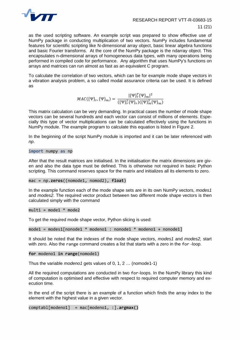
as the used scripting software. An example script was prepared to show effective use of NumPy package in conducting multiplication of two vectors. NumPy includes fundamental features for scientific scripting like N-dimensional array object, basic linear algebra functions and basic Fourier transforms. At the core of the NumPy package is the ndarray object. This encapsulates n-dimensional arrays of homogeneous data types, with many operations being performed in compiled code for performance. Any algorithm that uses NumPy’s functions on arrays and matrices can run almost as fast as an equivalent C program.

To calculate the correlation of two vectors, which can be for example mode shape vectors in a vibration analysis problem, a so called modal assurance criteria can be used. It is defined as

𝑀𝑀𝑀𝑀𝑀𝑀({Ψ}𝑟𝑟, {Ψ}𝑚𝑚) = |{Ψ}𝑟𝑟𝑇𝑇{Ψ}𝑚𝑚|2

({Ψ}𝑟𝑟𝑇𝑇{Ψ}𝑟𝑟)({Ψ}𝑚𝑚𝑇𝑇 {Ψ}𝑚𝑚)

This matrix calculation can be very demanding. In practical cases the number of mode shape vectors can be several hundreds and each vector can consist of millions of elements. Espe-cially this type of vector multiplications can be calculated effectively using the functions in NumPy module. The example program to calculate this equation is listed in Figure 2.

In the beginning of the script NumPy module is imported and it can be later referenced with np.

import numpy as np

After that the result matrices are initialised. In the initialisation the matrix dimensions are giv-en and also the data type must be defined. This is otherwise not required in basic Python scripting. This command reserves space for the matrix and initializes all its elements to zero.

mac = np.zeros((nomode1, nomod2), float)

In the example function each of the mode shape sets are in its own NumPy vectors, modes1 and modes2. The required vector product between two different mode shape vectors is then calculated simply with the command

multi = mode1 * mode2

To get the required mode shape vector, Python slicing is used:

mode1 = modes1[nonode1 * modeno1 : nonode1 * modeno1 + nonode1]

It should be noted that the indexes of the mode shape vectors, modes1 and modes2, start with zero. Also the range command creates a list that starts with a zero in the for -loop.

for modeno1 in range(nomode1)

Thus the variable modeno1 gets values of 0, 1, 2 … (nomode1-1)

All the required computations are conducted in two for-loops. In the NumPy library this kind of computation is optimised and effective with respect to required computer memory and ex-ecution time.

In the end of the script there is an example of a function which finds the array index to the element with the highest value in a given vector.

comptabl[modeno1] = mac[modeno1, :].argmax()


12 (21)

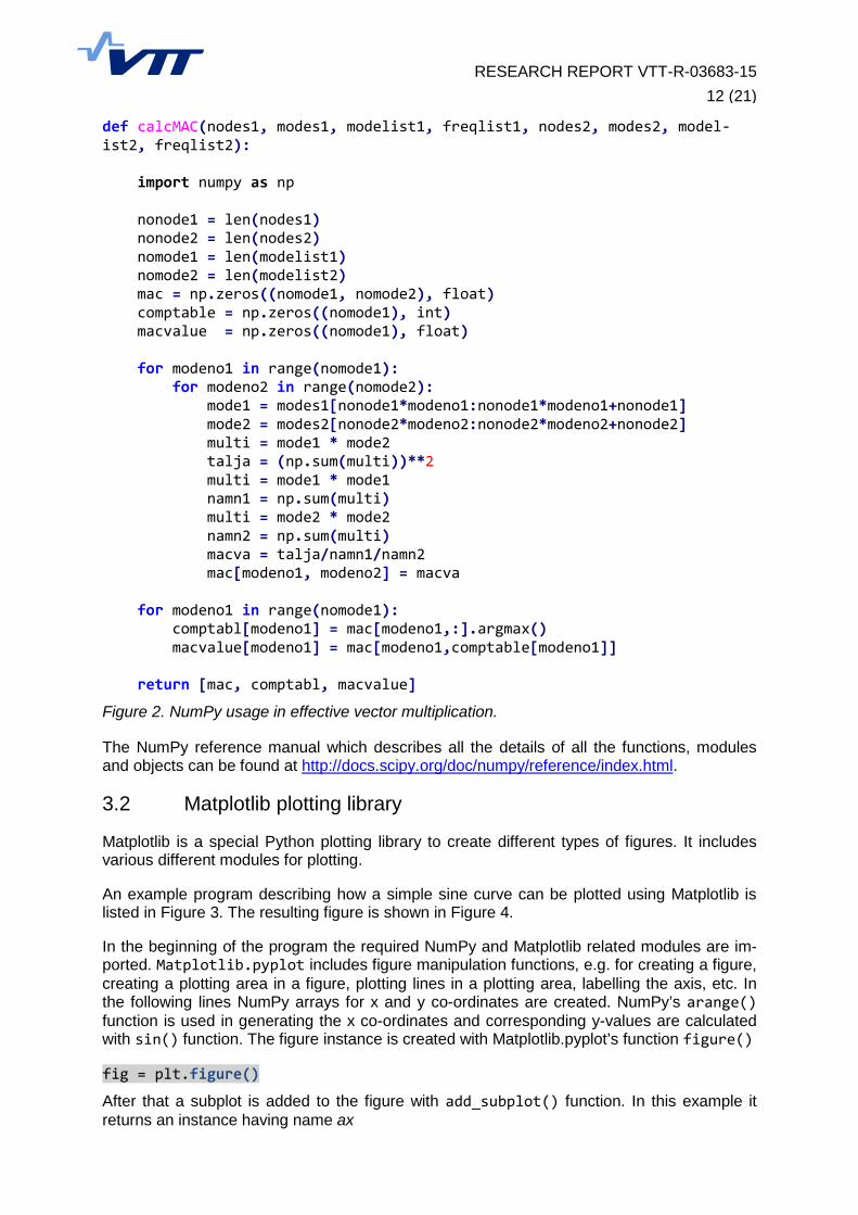
def calcMAC(nodes1, modes1, modelist1, freqlist1, nodes2, modes2, model-ist2, freqlist2): import numpy as np nonode1 = len(nodes1) nonode2 = len(nodes2) nomode1 = len(modelist1) nomode2 = len(modelist2) mac = np.zeros((nomode1, nomode2), float) comptable = np.zeros((nomode1), int) macvalue = np.zeros((nomode1), float) for modeno1 in range(nomode1): for modeno2 in range(nomode2): mode1 = modes1[nonode1*modeno1:nonode1*modeno1+nonode1] mode2 = modes2[nonode2*modeno2:nonode2*modeno2+nonode2] multi = mode1 * mode2 talja = (np.sum(multi))**2 multi = mode1 * mode1 namn1 = np.sum(multi) multi = mode2 * mode2 namn2 = np.sum(multi) macva = talja/namn1/namn2 mac[modeno1, modeno2] = macva for modeno1 in range(nomode1): comptabl[modeno1] = mac[modeno1,:].argmax() macvalue[modeno1] = mac[modeno1,comptable[modeno1]] return [mac, comptabl, macvalue]

Figure 2. NumPy usage in effective vector multiplication.

The NumPy reference manual which describes all the details of all the functions, modules and objects can be found at http://docs.scipy.org/doc/numpy/reference/index.html.

3.2 Matplotlib plotting library

Matplotlib is a special Python plotting library to create different types of figures. It includes various different modules for plotting.

An example program describing how a simple sine curve can be plotted using Matplotlib is listed in Figure 3. The resulting figure is shown in Figure 4.

In the beginning of the program the required NumPy and Matplotlib related modules are im-ported. Matplotlib.pyplot includes figure manipulation functions, e.g. for creating a figure, creating a plotting area in a figure, plotting lines in a plotting area, labelling the axis, etc. In the following lines NumPy arrays for x and y co-ordinates are created. NumPy’s arange() function is used in generating the x co-ordinates and corresponding y-values are calculated with sin() function. The figure instance is created with Matplotlib.pyplot’s function figure()

fig = plt.figure()

After that a subplot is added to the figure with add_subplot() function. In this example it returns an instance having name ax

http://docs.scipy.org/doc/numpy/reference/index.html


13 (21)

ax = fig.add_subplot(111)

In the following lines the curve is plotted and axis limits and labels are given. Finally, show() function is given to display the plot in the figure.

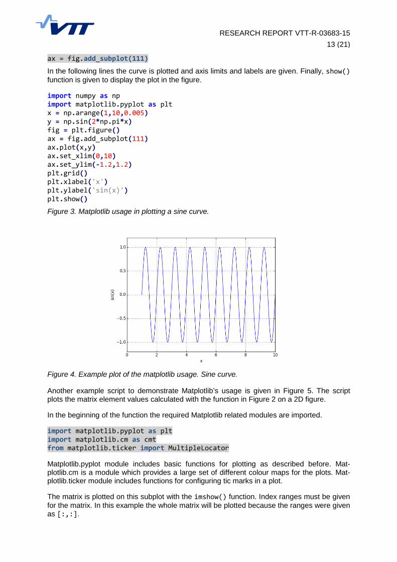
import numpy as np import matplotlib.pyplot as plt x = np.arange(1,10,0.005) y = np.sin(2*np.pi*x) fig = plt.figure() ax = fig.add_subplot(111) ax.plot(x,y) ax.set_xlim(0,10) ax.set_ylim(-1.2,1.2) plt.grid() plt.xlabel('x') plt.ylabel('sin(x)') plt.show()

Figure 3. Matplotlib usage in plotting a sine curve.

Figure 4. Example plot of the matplotlib usage. Sine curve.

Another example script to demonstrate Matplotlib’s usage is given in Figure 5. The script plots the matrix element values calculated with the function in Figure 2 on a 2D figure.

In the beginning of the function the required Matplotlib related modules are imported.

import matplotlib.pyplot as plt import matplotlib.cm as cmt from matplotlib.ticker import MultipleLocator

Matplotlib.pyplot module includes basic functions for plotting as described before. Mat-plotlib.cm is a module which provides a large set of different colour maps for the plots. Mat-plotlib.ticker module includes functions for configuring tic marks in a plot.

The matrix is plotted on this subplot with the imshow() function. Index ranges must be given for the matrix. In this example the whole matrix will be plotted because the ranges were given as [:,:].


14 (21)

cax = ax.imshow(matrix[:,:], cmap=cm.jet, interpolation = ’nearest’, origin=’lower’)

The figure can be saved with savefig() function. The file type is given in the file name.

plotfile = figurename + ‘.png’ plt.savefig(plotfile)

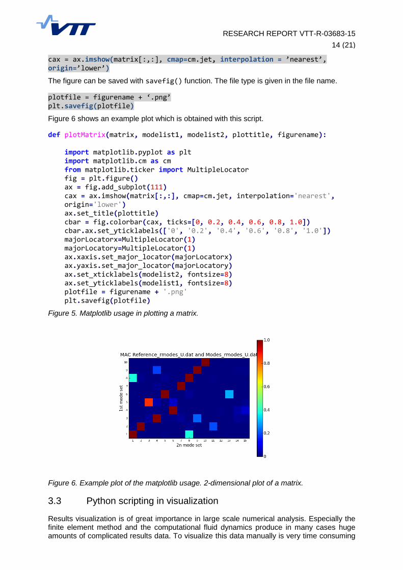
Figure 6 shows an example plot which is obtained with this script.

def plotMatrix(matrix, modelist1, modelist2, plottitle, figurename): import matplotlib.pyplot as plt import matplotlib.cm as cm from matplotlib.ticker import MultipleLocator fig = plt.figure() ax = fig.add_subplot(111) cax = ax.imshow(matrix[:,:], cmap=cm.jet, interpolation='nearest', origin='lower') ax.set_title(plottitle) cbar = fig.colorbar(cax, ticks=[0, 0.2, 0.4, 0.6, 0.8, 1.0]) cbar.ax.set_yticklabels(['0', '0.2', '0.4', '0.6', '0.8', '1.0']) majorLocatorx=MultipleLocator(1) majorLocatory=MultipleLocator(1) ax.xaxis.set_major_locator(majorLocatorx) ax.yaxis.set_major_locator(majorLocatory) ax.set_xticklabels(modelist2, fontsize=8) ax.set_yticklabels(modelist1, fontsize=8) plotfile = figurename + '.png' plt.savefig(plotfile)

Figure 5. Matplotlib usage in plotting a matrix.

Figure 6. Example plot of the matplotlib usage. 2-dimensional plot of a matrix.

3.3 Python scripting in visualization

Results visualization is of great importance in large scale numerical analysis. Especially the finite element method and the computational fluid dynamics produce in many cases huge amounts of complicated results data. To visualize this data manually is very time consuming


15 (21)

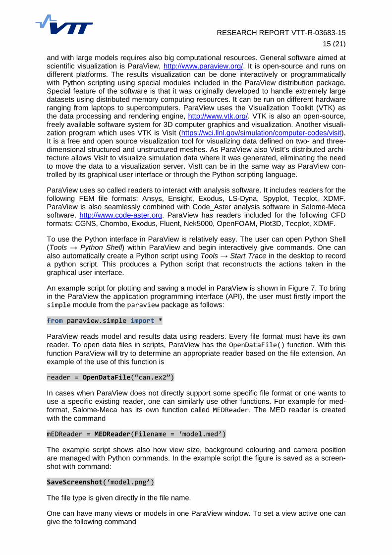
and with large models requires also big computational resources. General software aimed at scientific visualization is ParaView, http://www.paraview.org/. It is open-source and runs on different platforms. The results visualization can be done interactively or programmatically with Python scripting using special modules included in the ParaView distribution package. Special feature of the software is that it was originally developed to handle extremely large datasets using distributed memory computing resources. It can be run on different hardware ranging from laptops to supercomputers. ParaView uses the Visualization Toolkit (VTK) as the data processing and rendering engine, http://www.vtk.org/. VTK is also an open-source, freely available software system for 3D computer graphics and visualization. Another visuali-zation program which uses VTK is VisIt (https://wci.llnl.gov/simulation/computer-codes/visit). It is a free and open source visualization tool for visualizing data defined on two- and three-dimensional structured and unstructured meshes. As ParaView also VisIt’s distributed archi-tecture allows VisIt to visualize simulation data where it was generated, eliminating the need to move the data to a visualization server. VisIt can be in the same way as ParaView con-trolled by its graphical user interface or through the Python scripting language.

ParaView uses so called readers to interact with analysis software. It includes readers for the following FEM file formats: Ansys, Ensight, Exodus, LS-Dyna, Spyplot, Tecplot, XDMF. ParaView is also seamlessly combined with Code_Aster analysis software in Salome-Meca software, http://www.code-aster.org. ParaView has readers included for the following CFD formats: CGNS, Chombo, Exodus, Fluent, Nek5000, OpenFOAM, Plot3D, Tecplot, XDMF.

To use the Python interface in ParaView is relatively easy. The user can open Python Shell (Tools → Python Shell) within ParaView and begin interactively give commands. One can also automatically create a Python script using Tools → Start Trace in the desktop to record a python script. This produces a Python script that reconstructs the actions taken in the graphical user interface.

An example script for plotting and saving a model in ParaView is shown in Figure 7. To bring in the ParaView the application programming interface (API), the user must firstly import the simple module from the paraview package as follows:

from paraview.simple import *

ParaView reads model and results data using readers. Every file format must have its own reader. To open data files in scripts, ParaView has the OpenDataFile() function. With this function ParaView will try to determine an appropriate reader based on the file extension. An example of the use of this function is

reader = OpenDataFile(“can.ex2”)

In cases when ParaView does not directly support some specific file format or one wants to use a specific existing reader, one can similarly use other functions. For example for med-format, Salome-Meca has its own function called MEDReader. The MED reader is created with the command

mEDReader = MEDReader(Filename = ‘model.med’)

The example script shows also how view size, background colouring and camera position are managed with Python commands. In the example script the figure is saved as a screen-shot with command:

SaveScreenshot(‘model.png’)

The file type is given directly in the file name.

One can have many views or models in one ParaView window. To set a view active one can give the following command

http://www.paraview.org/

http://www.vtk.org/

https://wci.llnl.gov/simulation/computer-codes/visit

http://www.code-aster.org/


16 (21)

Show()

To make a view invisible there is the command

Hide()

To finally plot the figure one must give command

Render()

import pvsimple pvsimple.ShowParaviewView() #### import the simple module from the paraview from pvsimple import * #### disable automatic camera reset on 'Show' pvsimple._DisableFirstRenderCameraReset() # create a new 'MED Reader' mEDReader1 = MEDReader(FileName='model.med') # get active view renderView1 = GetActiveViewOrCreate('RenderView') # Set a specific view size renderView1.ViewSize = [1024, 600] # show data in view mEDReader1Display = Show(mEDReader1, renderView1) # get active view view = GetActiveView() # set gradient coloured background view.UseGradientBackground = True # set camera position view.CameraPosition = [1,0.5,1] SaveScreenshot('model.png') Show() Render()

Figure 7. Example Python script for ParaView.

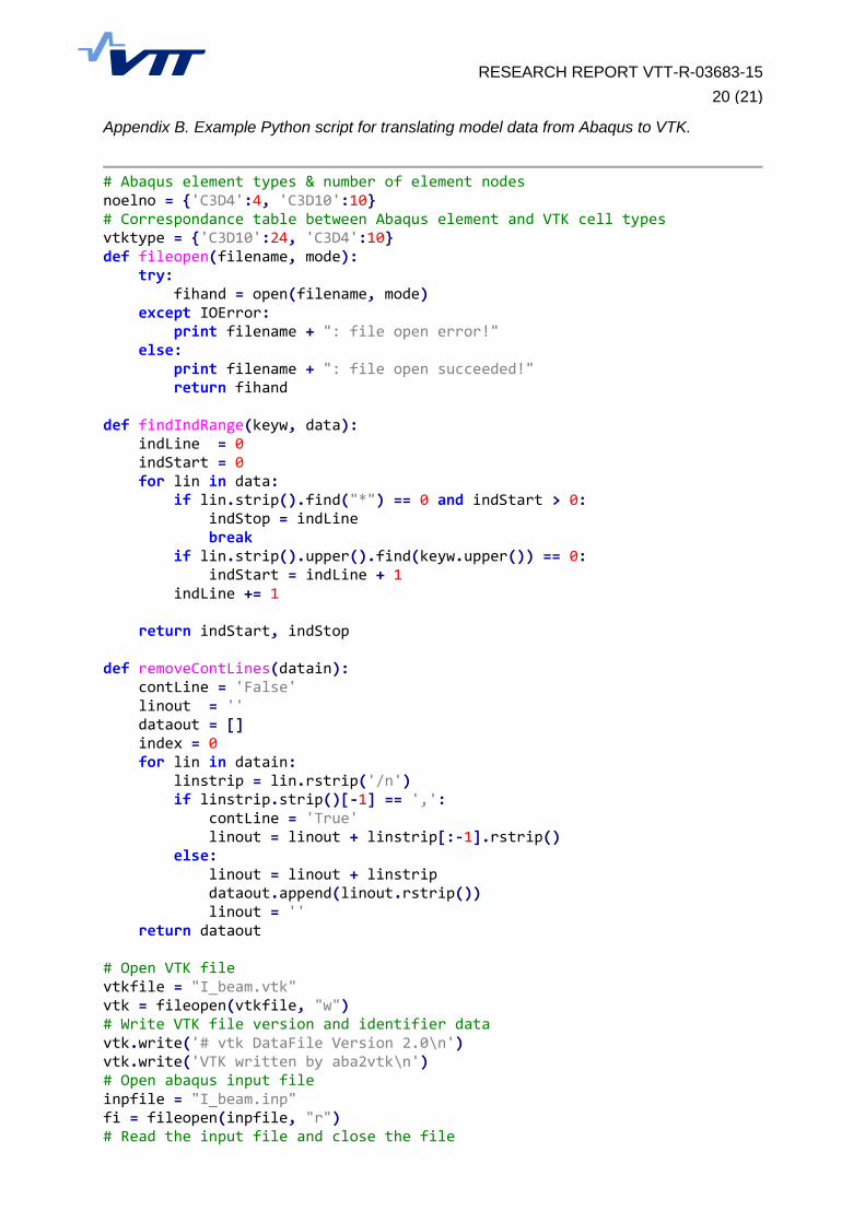
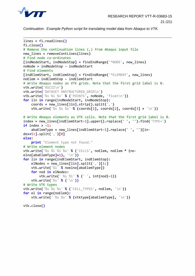
Although there are a wide range of readers for different software there might still remain a need to prepare user’s own reader. All the possibly software are not covered and especially for in-house software the creation of own readers might be necessary. Both ParaView and VisIt support the VTK file formats. VTK has relatively simple serial formats which are quite easy to read and write programmatically. Python scripting language is suitable for the prepa-ration of translators for model and results data from analysis software to VTK . As a simple example of such a program a short Python script is listed in Appendix B. It also serves as an example how basic Python commands for file handling, looping as well as control structures can be used in practice.

4. Conclusions

The use of scripting languages has become more and more popular in recent years. Espe-cially Python programming language has become the main scripting language of many commercial and non-commercial analysis software. Python is relatively easy to learn and use interactively. Moreover, basic programming does not necessary require any special devel-opment environment. The Python installation itself includes an integrated development envi-ronment which is called Python IDLE. It has already such good features that the basic Py-thon programming is effective. However, for more special programming needs there are vari-ous development environments available.


17 (21)

Although Python is easy to learn and use it is still a full-featured object oriented programming language having all the features that enable handling wide range of needs. For large scale scientific calculations the NumPy module enables effective calculations due to its special array class. Python is also an object-oriented language thus making possible the use of clas-ses and objects, if desired.

Interacting with commercial or non-commercial analysis software using Python is with some software possible. However, the use of special Python modules that are part of these soft-ware is in many cases not so simple. The programs have usually some kind of recording possibility which try to make the preparation of own scripts or macros more effective. Thus one sees directly the required commands and methods in the recorded script and the user needs only to modify the script to meet user’s own needs.


18 (21)

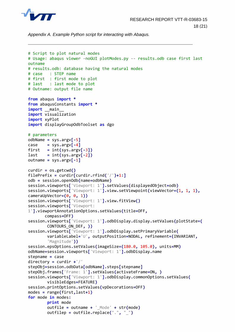
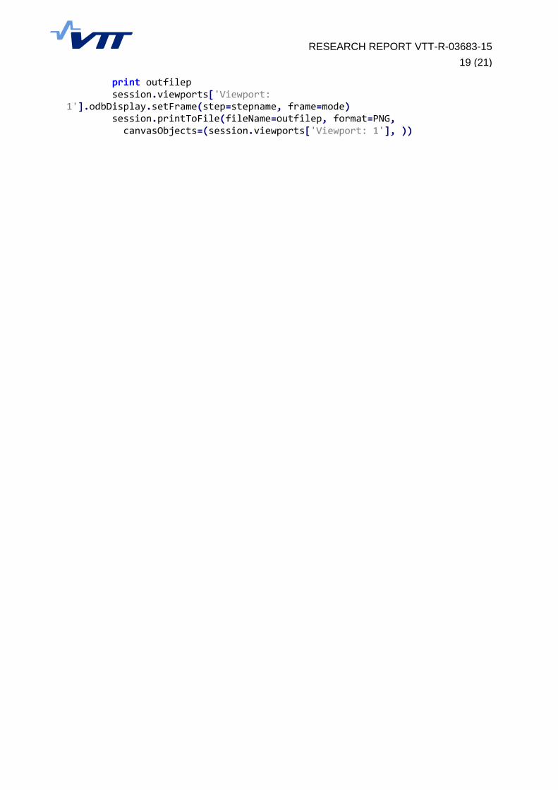
Appendix A. Example Python script for interacting with Abaqus.

# Script to plot natural modes # Usage: abaqus viewer -noGUI plotModes.py -- results.odb case first last outname # results.odb: database having the natural modes # case : STEP name # first : first mode to plot # last : last mode to plot # Outname: output file name from abaqus import * from abaqusConstants import * import __main__ import visualization import xyPlot import displayGroupOdbToolset as dgo # parameters odbName = sys.argv[-5] case = sys.argv[-4] first = int(sys.argv[-3]) last = int(sys.argv[-2]) outname = sys.argv[-1] curdir = os.getcwd() filePrefix = curdir[curdir.rfind('/')+1:] odb = session.openOdb(name=odbName) session.viewports['Viewport: 1'].setValues(displayedObject=odb) session.viewports['Viewport: 1'].view.setViewpoint(viewVector=(1, 1, 1), cameraUpVector=(0, 0, 1)) session.viewports['Viewport: 1'].view.fitView() session.viewports['Viewport: 1'].viewportAnnotationOptions.setValues(title=OFF, compass=OFF) session.viewports['Viewport: 1'].odbDisplay.display.setValues(plotState=( CONTOURS_ON_DEF, )) session.viewports['Viewport: 1'].odbDisplay.setPrimaryVariable( variableLabel='U', outputPosition=NODAL, refinement=(INVARIANT, 'Magnitude')) session.epsOptions.setValues(imageSize=(180.0, 105.0), units=MM) odbName=session.viewports['Viewport: 1'].odbDisplay.name stepname = case directory = curdir +'/' stepObj=session.odbData[odbName].steps[stepname] stepObj.frames['Frame: 1'].setValues(activateFrame=ON, ) session.viewports['Viewport: 1'].odbDisplay.commonOptions.setValues( visibleEdges=FEATURE) session.printOptions.setValues(vpDecorations=OFF) modes = range(first,last+1) for mode in modes: print mode outfile = outname + '_Mode' + str(mode) outfilep = outfile.replace(".", "_")


19 (21)

print outfilep session.viewports['Viewport: 1'].odbDisplay.setFrame(step=stepname, frame=mode) session.printToFile(fileName=outfilep, format=PNG, canvasObjects=(session.viewports['Viewport: 1'], ))


20 (21)

Appendix B. Example Python script for translating model data from Abaqus to VTK.

# Abaqus element types & number of element nodes noelno = {'C3D4':4, 'C3D10':10} # Correspondance table between Abaqus element and VTK cell types vtktype = {'C3D10':24, 'C3D4':10} def fileopen(filename, mode): try: fihand = open(filename, mode) except IOError: print filename + ": file open error!" else: print filename + ": file open succeeded!" return fihand def findIndRange(keyw, data): indLine = 0 indStart = 0 for lin in data: if lin.strip().find("*") == 0 and indStart > 0: indStop = indLine break if lin.strip().upper().find(keyw.upper()) == 0: indStart = indLine + 1 indLine += 1 return indStart, indStop def removeContLines(datain): contLine = 'False' linout = '' dataout = [] index = 0 for lin in datain: linstrip = lin.rstrip('/n') if linstrip.strip()[-1] == ',': contLine = 'True' linout = linout + linstrip[:-1].rstrip() else: linout = linout + linstrip dataout.append(linout.rstrip()) linout = '' return dataout # Open VTK file vtkfile = "I_beam.vtk" vtk = fileopen(vtkfile, "w") # Write VTK file version and identifier data vtk.write('# vtk DataFile Version 2.0\n') vtk.write('VTK written by aba2vtk\n') # Open abaqus input file inpfile = "I_beam.inp" fi = fileopen(inpfile, "r") # Read the input file and close the file


21 (21)

Continuation: Example Python script for translating model data from Abaqus to VTK.

lines = fi.readlines() fi.close() # Remove the continuation lines (,) from Abaqus input file new_lines = removeContLines(lines) # Find node co-ordinates [indNodeStart, indNodeStop] = findIndRange('*NODE', new_lines) noNode = indNodeStop - indNodeStart # Find elements [indElemStart, indElemStop] = findIndRange('*ELEMENT', new_lines) noElem = indElemStop - indElemStart # Write Abaqus nodes as VTK grids. Note that the first grid label is 0. vtk.write('ASCII\n') vtk.write('DATASET UNSTRUCTURED_GRID\n') vtk.write('%s %i %s' % ('POINTS', noNode, 'float\n')) for lin in range(indNodeStart, indNodeStop): coords = new_lines[lin].strip().split(',') vtk.write('%s %s %s' % (coords[1], coords[2], coords[3] + '\n')) # Write Abaqus elements as VTK cells. Note that the first grid label is 0. index = new_lines[indElemStart-1].upper().replace(" ", "").find('TYPE=') if index > -1: abaElemType = new_lines[indElemStart-1].replace(" ", "")[in-dex+5:].split(',')[0] else: print "Element type not found." # Write element nodes vtk.write('%s %i %i %s' % ('CELLS', noElem, noElem * (no-elno[abaElemType]+1), '\n')) for lin in range(indElemStart, indElemStop): elNodes = new_lines[lin].split(',')[1:] vtk.write('%i' % noelno[abaElemType]) for nod in elNodes: vtk.write(' %s %i' % (' ', int(nod)-1)) vtk.write('%s' % ('\n')) # Write VTK types vtk.write('%s %s %s' % ('CELL_TYPES', noElem, '\n')) for el in range(noElem): vtk.write(' %s %s' % (vtktype[abaElemType], '\n')) vtk.close()

Documents

Scripting in high performance computing environment