SCS-CN parameter determination using rainfall-runoff … · Earth Syst. Sci., 16, ... SCS-CN parameter determination using rainfall-runoff data in ... approach is widely used as a

Hydrol. Earth Syst. Sci., 16, 1001–1015, 2012www.hydrol-earth-syst-sci.net/16/1001/2012/doi:10.5194/hess-16-1001-2012© Author(s) 2012. CC Attribution 3.0 License.

Hydrology andEarth System

Sciences

SCS-CN parameter determination using rainfall-runoff data inheterogeneous watersheds – the two-CN system approach

K. X. Soulis and J. D. Valiantzas

Agricultural University of Athens, Department of Natural Resources Management and Agricultural Engineering,Division of Water Resources Management, Athens, Greece

Correspondence to:K. X. Soulis ([email protected])

Received: 5 September 2011 – Published in Hydrol. Earth Syst. Sci. Discuss.: 5 October 2011Revised: 1 February 2012 – Accepted: 16 March 2012 – Published: 28 March 2012

Abstract. The Soil Conservation Service Curve Number(SCS-CN) approach is widely used as a simple method forpredicting direct runoff volume for a given rainfall event.The CN parameter values corresponding to various soil, landcover, and land management conditions can be selected fromtables, but it is preferable to estimate the CN value from mea-sured rainfall-runoff data if available. However, previous re-searchers indicated that the CN values calculated from mea-sured rainfall-runoff data vary systematically with the rain-fall depth. Hence, they suggested the determination of asingle asymptotic CN value observed for very high rainfalldepths to characterize the watersheds’ runoff response. Inthis paper, the hypothesis that the observed correlation be-tween the calculated CN value and the rainfall depth in awatershed reflects the effect of soils and land cover spatialvariability on its hydrologic response is being tested. Basedon this hypothesis, the simplified concept of a two-CN het-erogeneous system is introduced to model the observed CN-rainfall variation by reducing the CN spatial variability intotwo classes. The behaviour of the CN-rainfall function pro-duced by the simplified two-CN system is approached theo-retically, it is analysed systematically, and it is found to besimilar to the variation observed in natural watersheds. Syn-thetic data tests, natural watersheds examples, and detailedstudy of two natural experimental watersheds with knownspatial heterogeneity characteristics were used to evaluatethe method. The results indicate that the determination ofCN values from rainfall runoff data using the proposed two-CN system approach provides reasonable accuracy and itover performs the previous methods based on the determi-nation of a single asymptotic CN value. Although the sug-gested method increases the number of unknown parametersto three (instead of one), a clear physical reasoning for themis presented.

1 Introduction

Simple methods for predicting runoff from watersheds areparticularly important in hydrologic engineering and hydro-logical modelling and they are used in many hydrologic ap-plications, such as flood design and water balance calcula-tion models (Abon et al., 2011; Steenhuis et al., 1995; vanDijk, 2010). The Soil Conservation Service Curve Num-ber (SCS-CN) method was originally developed by the SCS(US Department of Agriculture), to predict direct runoff vol-umes for given rainfall events and it is documented in the Na-tional Engineering Handbook, Sect. 4: Hydrology (NEH-4)(SCS, 1956, 1964, 1971, 1985, 1993, 2004). It soon becameone of the most popular techniques among the engineers andthe practitioners, because it is a simple but well-establishedmethod, it features easy to obtain and well-documented en-vironmental inputs, and it accounts for many of the factorsaffecting runoff generation, incorporating them in a singleCN parameter. In contrast, the main weaknesses reportedin the literature are that the SCS-CN method does not con-sider the impact of rainfall intensity, it does not addressthe effects of spatial scale, it is highly sensitive to changesin values of its single parameter, CN, and it is ambigu-ous considering the effect of antecedent moisture conditions(Hawkins, 1993; McCuen, 2002; Michel et al., 2005; Ponceand Hawkins, 1996).

The SCS-CN method was soon adopted for various re-gions, land uses and climate conditions (Elhakeem and Pa-panicolaou, 2009; King and Balogh, 2008; Mishra andSingh, 1999; Romero et al., 2007). It was also evolved wellbeyond its original scope and it became an integral part ofcontinuous simulation models (e.g. Adornado and Yoshida,2010; Holman et al., 2003; Mishra and Singh, 2004; Morettiand Montanari, 2008; Soulis and Dercas, 2007). Many

Published by Copernicus Publications on behalf of the European Geosciences Union.

1002 K. X. Soulis and J. D. Valiantzas: The two-CN system approach

studies aiming at finding a theoretical basis for the method,facilitating its use in regions and for climate conditions notpreviously evaluated, and supporting its further improve-ment, were carried out as well (Hjelmfelt, 1991; Tramblayet al., 2010; Yu, 1998).

However, in spite of its widespread use, there is not anagreed methodology to estimate the CN parameter valuesfrom measured rainfall runoff data. Such a method would beimportant for two main purposes: (a) it would allow the deter-mination of the CN parameter values from measured rainfallrunoff data of local or nearby similar watersheds when suit-able data were available and (b) it would facilitate studiesaiming at the extension of the SCS-CN method documen-tation for different, soil, land use, and climate conditions.Though, the main difficulty is that the CN values calculatedfrom measured rainfall runoff data actually vary significantlyfrom storm to storm on any watershed. This effect posed indoubt the adequacy of curve number model itself to predictrunoff. Antecedent Moisture Condition (AMC) was initiallyassumed to be the primary cause of storm to storm varia-tion. However, this effect is of questionable origin and it isnot recommended for use anymore (Hjelmfelt et al., 2001;McCuen, 2002; Ponce and Hawkins, 1996). In the latest ver-sion of the NEH-4 the reference to AMC was revised as fol-lows. Variability is incorporated by considering the CN as arandom variable and the AMC-I and AMC-III categories asbounds of the distribution. The expressions of AMC-I andAMC-III were considered as measures of dispersion aroundthe constant tendency (AMC-II) (Hjelmfelt et al., 2001).

Ponce and Hawkins (1996) reported as possible sourcesof this variability the effect of the temporal and spatial vari-ability of storm and watershed properties, the quality of themeasured data, and the effect of antecedent rainfall and as-sociated soil moisture. Soulis et al. (2009) and Steenhuis etal. (1995) also noted that the variation of CN value, accord-ing to AMC category alone, cannot justify the observed CNvalues variability in every case.

Hawkins (1993) in his study on the asymptotic determina-tion of runoff curve numbers from measured runoff analysinga significantly large number of watersheds, where CNs arecalculated from real rainfall-runoff data, concluded that asecondary systematic correlation almost always emerges inwatersheds between the calculated CN value and the rainfalldepth. In most of the watersheds, these calculated CNs ap-proach a constant value with increasing rainfall depth thatis assumed to characterize the watershed. The three dif-ferent behaviours that have been observed are described asfollows: the most common scenario is that at small rainfalldepths correspond larger values of calculated CNs, which de-cline progressively with increasing storm size, approaching astable near constant asymptotic CN value with increasinglylarger storms. This behaviour appears most frequently andit is characterized as “standard”. An example of this patternis given in Fig. 1. Hawkins (1993) suggests the identifica-tion of a single asymptotic CN value observed for very large

27

Figures 1

4 0

5 0

6 0

7 0

8 0

9 0

1 0 0

0 5 0 1 0 0 1 5 0 2 0 0R ainfall (m m )

CN

Va

lue

α=0 .0 1 C Nα=9 3 C Nb=4 6 (R 2=0 .9 9 8 )α=0 .1 1 C Nα=8 2 C Nb=4 8 (R 2=0 .9 9 3 )C o m p lac e nt b e havio urS tand ard b e havio urE nve lo p e c urve

2

Figure 1. Two-CN system model curves fitted to the data presented by Hawkins (1993) for the 3

“Standard” (Coweeta watershed #2, North Carolina) and the “complacent” (West Donaldson 4

Creek, Oregon) behaviour watersheds. 5

6

Fig. 1. Two-CN system model curves fitted to the data presented byHawkins (1993) for the “standard” (Coweeta watershed #2, NorthCarolina) and the “complacent” (West Donaldson Creek, Oregon)behaviour watersheds.

storm sizes to characterize such watersheds. In less commoncases of watersheds the observed CN declines steadily withincreasing rainfall with no appreciable tendency to approacha constant value (“complacent” behaviour, Fig. 1). Accord-ing to Hawkins (1993), an asymptotic CN cannot be safelydetermined from data for this behaviour. In the last case,concerning also a small number of watersheds, the calculatedCNs have an apparently constant value for all rainfall depthsexcept very low rainfall depths where CN increases suddenly(“violent” behaviour).

Additional examples of watersheds featuring similarbehaviours are presented by Hjelmfeld et al. (2001).Bonta (1997) proposed an improvement to theHawkins (1993) method for the asymptotic determina-tion of CNs from measured data in “violent” and “standard”watersheds using derived distributions.

All previously developed methodologies for estimatingCNs from measured data focus mainly on the determinationof a single asymptotic CN value characterizing the water-shed hydrologic response for high rainfall depths. The ob-served deviations from the asymptotic behaviour for lowerrainfall depths are not essentially taken into considerationand are rather attributed to various sources of temporal vari-ability. For this reason, the resulting CN values fail to de-scribe the watershed response in small and medium rainfallevents, limiting the applicability of the method to its origi-nal scope, namely the estimation of peak runoff values. Fur-thermore, the above methods fail to determine a final CNvalue in “complacent” watersheds. The CN varies as a func-tion of the soil infiltration capacity and the land cover of thewatershed, which are two essentially time invariant factors.

Hydrol. Earth Syst. Sci., 16, 1001–1015, 2012 www.hydrol-earth-syst-sci.net/16/1001/2012/

K. X. Soulis and J. D. Valiantzas: The two-CN system approach 1003

Various sources of temporal variability, such as the effect ofspatio-temporal rainfall intensity variability, the effect of an-tecedent rainfall, etc., make CN to be considered as a randomvariable with bounds of distribution AMC-I and AMC-III.The SCS-CN method was originally developed as a lumpedmodel and up to this date it is still primarily used as a lumpedmodel. In natural watersheds, however, spatial variability (atlower or higher level) with regard to the soil-cover complex isinevitable (such spatial heterogeneity in the watershed couldbe considered temporally invariant).

In this paper, a novel hypothesis is proposed suggestingthat the intrinsic correlation between calculated CN valueand rainfall depth observed in watersheds corresponding tothe “standard” and “complacent” cases is essentially the nat-ural consequence of the presence of soils and land cover spa-tial variability along the watersheds. It is shown that thepresence of spatial variability (at low or high level) in thewatersheds produces a progressive decrease in the calculatedCNs as the storm size decreases and for excessively largestorm sizes the CN tends to stabilize in an asymptotic CNvalue. The proposed hypothesis is approached theoretically,it is analysed systematically using synthetic data, it is studiedin two natural experimental watersheds with known spatialheterogeneity characteristics and it is evaluated using nat-ural watersheds examples. The results of the analysis pro-vide evidence that the spatial variability of the watershed caninfluence the CN determination procedure from measuredrainfall-runoff data and that the estimation of more than oneCN values is needed in order to describe the spatial variabil-ity of the watershed and to facilitate the determination proce-dure. Based on the above hypothesis, the simplified conceptof an equivalent two-CN heterogeneous system is introducedto model the CN vs. rainfall depth variation. This new evo-lution takes into consideration the soil-cover complex spa-tial variation in the estimation of CN values from measuredrainfall-runoff data, in order to extend the applicability of theSCS-CN method for a wider range of rainfall depths and toprovide improved simulations in heterogeneous watersheds.

2 Theoretical development

2.1 SCS-CN method

The SCS-CN method is based on the following basic formcalculating runoff from rainfall depth,

Q =(P −Ia)

2

P −Ia+Sfor P >Ia

Q = 0 for P ≤ Ia (1)

whereP is the total rainfall,Ia is the initial abstraction,Q isthe direct runoff andS is the potential maximum retention.Based on a second assumption, that the amount of initial ab-straction is a fraction of the potential maximum retention

Ia= λS (2)

Eq. (1) becomes

Q =(P −λS)2

P +(1−λ)S(3)

The potential retentionS is expressed in terms of the dimen-sionless curve number (CN) through the relationship

S =1000

CN−10 (4a)

taking values from 0, whenS → ∞, to 100, whenS = 0.This definition was originally applied to the English metricsystem (withS in inches). In the SI units (withS in mm) thefollowing definition should be used:

S =25 400

CN−254 (4b)

The determination of all the NEH-4 SCS-CN values com-monly used in hydrologic practice, assume the initial ab-straction rate to be set to the constant value,λ = 0.2, in or-der thatS (or its transformation CN) remains the only freeunknown parameter of the method. Recently, Woodward etal. (2003) analysing event rainfall-runoff data from severalhundred plots recommended usingλ = 0.05.

The CN values corresponding to the various soil types,land cover and land management conditions can be selectedfrom the NEH-4 tables. However, it is preferable to esti-mate the CN value from recorded rainfall-runoff data fromlocal or nearby similar watersheds. When rainfall-runoff dataare available for a watershed,P and Q pairs are used di-rectly to determine the potential retentionS characterizingthe watershed (Chen, 1982)

S =P

λ+

(1−λ)Q−

√(1−λ)2Q2+4λPQ

2λ2(5)

Combining Eq. (4b) with Eq. (5), CN value can be directlycalculated from rainfall-runoff data

CN=25 400

Pλ

+(1−λ)Q−

√(1−λ)2Q2+4λPQ

2λ2 +254(6)

2.2 Runoff prediction errors related to the use of singlecomposite CN values

Grove et al. (1998) in their study investigated the effect ofusing single composite CN values (i.e. the area-weighted av-erage of the CN values in the watershed) instead of weightedrunoff estimates, indicating that significant errors in runoffestimates can occur when composited rather than distributedCNs are used. Lantz and Hawkins (2001) also discussedthe possible errors caused by the use of a single compositeCN value.

The main reason for the errors produced using the compos-ite CN value instead of weighted-Q is the non-linear formof the SCS-CN formula. As an example, the case of a vir-tual watershed divided into two equal sub-areas characterized

www.hydrol-earth-syst-sci.net/16/1001/2012/ Hydrol. Earth Syst. Sci., 16, 1001–1015, 2012


28

1

Figure 2. Relative percentage error against the range of CN variation, for various total rainfall 2

depths and for various average CN values. 3

4

Fig. 2. Relative percentage error against the range of CN variation, for various total rainfall depths and for various average CN values.

by different CN values is illustrated in Fig. 2. In this figurethe relative percentage error of the runoff predictions usinga single composite CN value is plotted against the range ofCN variation, for various total rainfall depths and for vari-ous average CN values. The above figure clearly illustratesthat the percentage error increases as the range of CN varia-tion increases and decreases as the average CN value and therainfall depth increase. It is also clearly shown that for lowrainfall depths significant errors are observed, even for smallCN variation ranges. These results are in agreement with theresults of Grove et al. (1998).

2.3 The two-CN heterogeneous system

In order to investigate the consequence of spatial variabilityon the CN vs.P relationship in a watershed, in a first stageof the analysis it is assumed the simplified scheme, accordingto which the entire area of the watershed under considerationis composed from relatively homogeneous sub-areas. Eachsub-area is assigned a CN value obtained from a specific setof two CN values CNa and CNb with CNa> CNb. If a de-notes the area fraction of the watershed with CN = CNa, then(1-a) is the area fraction of the watershed with CN = CNb. Itseems obvious that CN must be taken constant for a relativelyhomogeneous soil-cover complex. Various temporal effectssuch as the effect of the spatiotemporal variability of givenstorm, the effect of storm intensity, the effect of antecedentrainfall and others are considered as random effects on theCN calculation.

Traditionally the runoff equation for a heterogeneous wa-tershed is described by using a single composite value of thedifferent CN-areas, this being an area- weighted CN value.However, runoff is more accurately estimated using individu-ally calculated weighted runoff for the array of different sub-areas as it was shown in the previous section. Therefore, therunoff, Q responded to the causative rainfall event,P gen-erated by the two-CN system is described by the followingequation,

Q = 0 for P <λSa (7a)

Q = a(P −λSa)

2

[P +(1−λ)Sa]for λSa≤ P <λSb (7b)

Q = a(P −λSa)

2

[P +(1−λ)Sa]+(1−a)

(P −λSb)2

[P +(1−λ)Sb]for P ≥ λSb (7c)

whereSa andSb are the potential maximum retention val-ues corresponding to the two homogeneous sub-areas char-acterized by the CNα and CNb values respectively, andλ isa constant value (usuallyλ = 0.2 orλ = 0.05). Sa andSb arecalculated from the corresponding CN values using Eq. (4b).

Following, it will be pointed out that such a two-CN het-erogeneous system is characterized by a secondary relation-ship that always emerges between calculated CN and rainfalldepth,P. The particular behaviour of this relationship willbe analysed in detail as well.

It is considered that for various rainfall events of depthP, realized on the two-CN heterogeneous system, the corre-sponding “actual” observed runoff,Q, is obtained by Eq. (7a,b, c). Then the CN for this system can be calculated byEq. (6) containing onlyP andQ; thus any “realized”P -Qdata pair can be used to calculate what should be the CNfor that particular rainfall-runoff event in the heterogeneoussystem.

2.3.1 Large-P behaviour – Asymptotic CN

Equation (7c) can be standardized by using the reduced vari-ables (P/Sa), and (P/Sb), (Sa< Sb). The resulting relation-ship becomes:

Q = aSa(P/Sa−λ)2

[P/Sa+(1−λ)]+(1−a)Sb

(P/Sb−λ)2

[P/Sb+(1−λ)]for P ≥ λSb (8)

while using the auxiliary variablesX1 = P/Sa+ (1−λ) andX2 = P/Sb+(1−λ) Eq. (8) becomes

Q = aSa[X1+1/X1−2] +(1−a)Sb[X2+1/X2−2] (9)



For asymptotic large values ofP and consequently asymp-totic large values ofX1 andX2, the corresponding value ofQ∞ approaches asymptotically the value

Q∞ = aSa[P/Sa+(1−λ)] +(1−a)Sb[P/Sb+(1−λ)] (10)

or equivalently

Q∞ = P −(1−λ)[aSa+(1−a)Sb] (11)

By following a similar procedure assuming a perfectly uni-form watershed characterized by a single CN-value (or itssimple transformedS), the value ofQ∞ for large values ofP approaches asymptotically

Q∞ = P −(1−λ)S (12)

By puttingS∞ = aSa+(1−a)Sb in Eq. (11) the two-CN het-erogeneous system behave asymptotically for largeP val-ues as a single CN value system with equivalent potentialretentionS∞ and equivalent CN value

CN∞ =25 400

aSa+(1−a)Sb+254(13)

Only for large values ofP the heterogeneous system can becharacterized by a single asymptotic CN value that could beobtained using the specific “composite” CN value (Eq. 13).However, even in this case this asymptotic value does notcharacterize a single specific soil but it is the superpositionof different complexes.

Systematic analysis indicates that the value of CN∞ givenby Eq. (13) is sufficiently close to the usual composite CNvalue

CN∞ = aCNa+(1−a)CNb (14)

Further analysis based on systematic generation ofQ-P syn-thetic data for various combinations ofa, CNa and CNb in-put parameters characterizing the two-CN system indicatesthat CN approaches the asymptotic value given by Eq. (13)for unrealistic, extremely large values ofP , P > 3000 mm.Alternatively the CN approaches the composite asymptoticvalue given by Eq. (14) for more realistic large values ofP . Note that the composite value given by Eq. (14) is tra-ditionally used to characterize an heterogeneous system by asingle-CN value.

2.3.2 Low-P behaviour – Envelope curve

For a two-CN system, asP decreases the calculated valuesof CN increase, as illustrated in Fig. 3. For some thresholdvalue ofP ,

Po = λSa (15)

the CN value becomes maximum equal to the larger CN-category, CNa, whereas for any smallerP <Po value the CNis not defined since it will give no runoffQ = 0. Indeed for

29

40

50

60

70

80

90

100

0 50 100 150 200 250 300Ra infa ll (m m )

CN

val

ue

E nvelope C urve

α :0.9 C Nα:90 C Nb:65 α :0.5 C Nα:90 C Nb:65 α :0.1 C Nα:90 C Nb:65α :0.9 C Nα:90 C Nb:40 α :0.5 C Nα:90 C Nb:40 α :0.1 C Nα:90 C Nb:40α :0.9 C Nα:65 C Nb:40 α :0.5 C Nα:65 C Nb:40 α :0.1 C Nα:65 C Nb:40

25400

254CN Pο

ο

λ

=+

1

Figure 3. Calculated CN values against rainfall depth for various values of the a, CNa, and 2

CNb parameters. 3

4

Fig. 3. Calculated CN values against rainfall depth for various val-ues of thea, CNa, and CNb parameters.

P -Q pairs generated by Eq. (7a, b, c), whenP decreases ap-proaching asymptotically the value ofPo, thenQ → 0 there-fore the asymptotic threshold value ofS,So, calculated byEq. (5) is So = Po/λ. SinceSa is also given bySa = Po/λ,therefore the threshold value of CN, CNo = CNa. The valuesof threshold maximum curve number, CNo as function ofPois given as

CNo =25 400

254+Poλ

(16)

The threshold CNo(Po) curve is an envelope curve that couldbe interpreted as the intrinsic CN(P ) variation for a two-CNsystem with asymptotic characteristics CNa → 100, CNb →

0, anda → 0. It is the curve defining the position of maxCNo = CNa value at the thresholdP = Po=λSa (see Figs. 1and 3)

2.3.3 Illustration of the two-CN heterogeneous systembehaviour

In order to illustrate the behaviour of the secondary relation-ship between the calculated CN and the rainfall depth,P inthe above described two-CN heterogeneous system, “actual”observed runoff values,Q, were obtained by Eq. (7a, b, c)for various rainfall depthsP, by varying systematically thea, CNa, and CNb parameters. Then the corresponding CNvalues for this system were calculated by Eq. (6) and a seriesof CN-P curves were produced. It must be noticed that here-after, the standard case ofλ=0.2 is examined. However, thefollowing analysis is also valid for otherλ values, as well.

In Fig. 3 the calculated CN values for the various values ofa, CNa, and CNb parameters are plotted against the rainfalldepthP . In this figure, a significant variation of the esti-mated CN values for various rainfall depths can be observed.The variation increases as the difference between CNa and



Table 1. Characteristics of 21 examples of hypothetical watersheds that are characterized by three CN value categories and best fitted valuesof thea, CNa, and CNb parameters.

Actual values Fitted values(3 CN value categories) (Two-CN model)

no. Area (%) Cor. CN Values a CNα CNb R2

1 10 80 10 30 60 90 0.15 88 56 0.992 33 33 33 30 60 90 0.43 88 40 0.993 10 10 80 30 60 90 0.83 90 39 0.994 80 10 10 30 60 90 0.14 87 32 0.995 40 40 20 30 60 90 0.32 86 40 0.996 20 40 40 30 60 90 0.49 89 45 0.997 40 20 40 30 60 90 0.47 89 36 0.998 10 80 10 60 75 90 0.16 89 73 0.999 33 33 33 60 75 90 0.41 89 65 0.9910 10 10 80 60 75 90 0.82 90 65 0.9911 80 10 10 60 75 90 0.13 89 61 0.9912 40 40 20 60 75 90 0.29 89 65 0.9913 20 40 40 60 75 90 0.48 89 68 0.9914 40 20 40 60 75 90 0.45 90 63 0.9915 10 80 10 30 45 60 0.15 58 43 0.9916 33 33 33 30 45 60 0.44 59 35 0.9917 10 10 80 30 45 60 0.83 60 34 0.9918 80 10 10 30 45 60 0.14 58 31 0.9919 40 40 20 30 45 60 0.32 58 35 0.9920 20 40 40 30 45 60 0.5 59 37 0.9921 40 20 40 30 45 60 0.47 59 33 0.99

CNb parameters value increases and decreases as the rain-fall depth and the weighted CN value increase. It is clearlyshown as well that for very high weighted CN values, theestimated CN value is almost invariable. It can be observedthat the factors associated with significant variation of theestimated CN values for various rainfall depths, are also as-sociated with significant errors when runoff estimations aremade using composited rather than distributed CNs, as it wasshown in Sect. 2.2. This observation provides a strong indi-cation that the observed correlation between the calculatedCN values and the rainfall depth should be associated withthe presence of soil-cover complex spatial variability in thewatershed.

In Fig. 3 can be also observed that the shapes of theCN-P curves produced by the two-CN heterogeneous sys-tem are quite similar with the shapes of the “standard” and“complacent” watersheds correlation curves presented byHawkins (1993). WhenQ-P data are available, the two-CN system can be viewed as a fitting model to the trans-formed CN-P data with free parametersa, CNa, and CNb(the equations of the two-CN system fitting model that canbe used in a non-linear least squared procedure, are givenin the Appendix A). Thus, in order to highlight further thesimilarity observed in Fig. 3, the two-CN hypothetical wa-tershed curves were fitted to the CN-P curves presented by

Hawkins (1993) as examples of the “standard” (Coweeta wa-tershed #2, North Carolina) and of the “complacent” (WestDonaldson Creek, Oregon) behaviour, by adjusting the val-ues of thea, CNa, and CNb parameters. As it can be clearlyseen in Fig. 1, the CN-P curves are fitted very well by thetwo-CN system model in both cases. These results providefurther evidence that the spatial variability of the watershedcan influence the CN determination procedure. In this casethe estimation of more than one CN values is needed in or-der to describe the spatial variability of the watershed and tofacilitate the determination procedure.

2.4 Generalization

Although the previous analysis is initially restricted for two-CN idealized watershed examples, generally, in natural wa-tersheds could appear more than two CN value categories.However, every added CN category requires the determina-tion of two more parameters (the corresponding CN valueand the area it covers), giving rise to the overparameteriza-tion problem. Therefore, in a second stage it is investigatedif a heterogeneous watershed characterized by three differentCN values can be approached with sufficient accuracy usingtwo CN value categories.



30

1

Figure 4. Two-CN system model curves fitted to the synthetic rainfall–CN data created for the 2

21 examples of hypothetical watersheds that are characterized by three CN value categories as 3

described in Table 1. 4

5

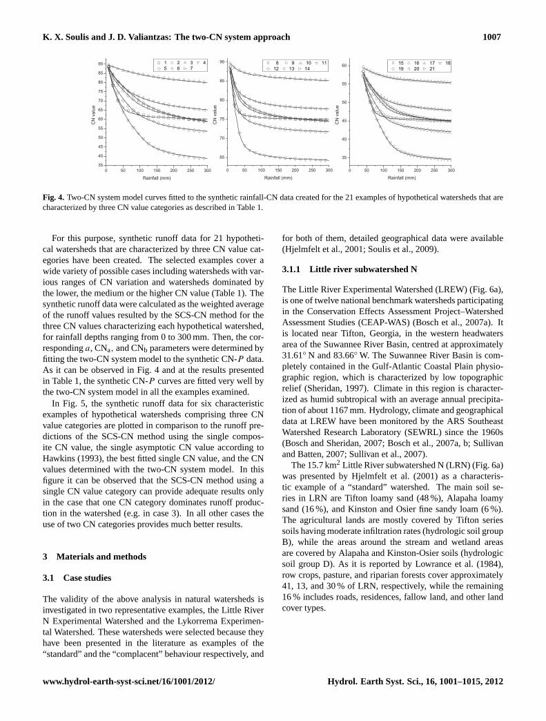
Fig. 4. Two-CN system model curves fitted to the synthetic rainfall-CN data created for the 21 examples of hypothetical watersheds that arecharacterized by three CN value categories as described in Table 1.

For this purpose, synthetic runoff data for 21 hypotheti-cal watersheds that are characterized by three CN value cat-egories have been created. The selected examples cover awide variety of possible cases including watersheds with var-ious ranges of CN variation and watersheds dominated bythe lower, the medium or the higher CN value (Table 1). Thesynthetic runoff data were calculated as the weighted averageof the runoff values resulted by the SCS-CN method for thethree CN values characterizing each hypothetical watershed,for rainfall depths ranging from 0 to 300 mm. Then, the cor-respondinga, CNa, and CNb parameters were determined byfitting the two-CN system model to the synthetic CN-P data.As it can be observed in Fig. 4 and at the results presentedin Table 1, the synthetic CN-P curves are fitted very well bythe two-CN system model in all the examples examined.

In Fig. 5, the synthetic runoff data for six characteristicexamples of hypothetical watersheds comprising three CNvalue categories are plotted in comparison to the runoff pre-dictions of the SCS-CN method using the single compos-ite CN value, the single asymptotic CN value according toHawkins (1993), the best fitted single CN value, and the CNvalues determined with the two-CN system model. In thisfigure it can be observed that the SCS-CN method using asingle CN value category can provide adequate results onlyin the case that one CN category dominates runoff produc-tion in the watershed (e.g. in case 3). In all other cases theuse of two CN categories provides much better results.

3 Materials and methods

3.1 Case studies

The validity of the above analysis in natural watersheds isinvestigated in two representative examples, the Little RiverN Experimental Watershed and the Lykorrema Experimen-tal Watershed. These watersheds were selected because theyhave been presented in the literature as examples of the“standard” and the “complacent” behaviour respectively, and

for both of them, detailed geographical data were available(Hjelmfelt et al., 2001; Soulis et al., 2009).

3.1.1 Little river subwatershed N

The Little River Experimental Watershed (LREW) (Fig. 6a),is one of twelve national benchmark watersheds participatingin the Conservation Effects Assessment Project–WatershedAssessment Studies (CEAP-WAS) (Bosch et al., 2007a). Itis located near Tifton, Georgia, in the western headwatersarea of the Suwannee River Basin, centred at approximately31.61◦ N and 83.66◦ W. The Suwannee River Basin is com-pletely contained in the Gulf-Atlantic Coastal Plain physio-graphic region, which is characterized by low topographicrelief (Sheridan, 1997). Climate in this region is character-ized as humid subtropical with an average annual precipita-tion of about 1167 mm. Hydrology, climate and geographicaldata at LREW have been monitored by the ARS SoutheastWatershed Research Laboratory (SEWRL) since the 1960s(Bosch and Sheridan, 2007; Bosch et al., 2007a, b; Sullivanand Batten, 2007; Sullivan et al., 2007).

The 15.7 km2 Little River subwatershed N (LRN) (Fig. 6a)was presented by Hjelmfelt et al. (2001) as a characteris-tic example of a “standard” watershed. The main soil se-ries in LRN are Tifton loamy sand (48 %), Alapaha loamysand (16 %), and Kinston and Osier fine sandy loam (6 %).The agricultural lands are mostly covered by Tifton seriessoils having moderate infiltration rates (hydrologic soil groupB), while the areas around the stream and wetland areasare covered by Alapaha and Kinston-Osier soils (hydrologicsoil group D). As it is reported by Lowrance et al. (1984),row crops, pasture, and riparian forests cover approximately41, 13, and 30 % of LRN, respectively, while the remaining16 % includes roads, residences, fallow land, and other landcover types.



31

1

Figure 5. Synthetic runoff data in comparison to the runoff predictions of the SCS-CN method 2

using the single composite CN value, the single asymptotic CN value according to Hawkins 3

(1993), the best fitted CN value, and the proposed two-CN system model, for six 4

characteristic cases as described in Table 1. 5

6

Fig. 5. Synthetic runoff data in comparison to the runoff predictions of the SCS-CN method using the single composite CN value, the singleasymptotic CN value according to Hawkins (1993), the best fitted CN value, and the proposed two-CN system model, for six characteristiccases as described in Table 1.

32

1

Figure 6. Map of the case study sites: (a) LRN watershed, (b) Lykorrema experimental 2

watershed. 3

4

Fig. 6. Map of the case study sites:(a) LRN watershed,(b) Lykor-rema experimental watershed.

3.1.2 Lykorrema, Penteli

The small scale experimental watershed of Lykorrema stream(15.2 km2), situated in the east side of Penteli Mountain, At-tica, Greece, centred at approximately 38.02◦ N and 23.55◦ E(Fig. 6b). The watershed is divided in two sub-watersheds.The Upper Lykorrema watershed (7.84 km2) and the LowerLykorrema watershed (7.36 km2). The Upper and LowerLykorrema experimental watersheds are operated from theAgricultural University of Athens, Greece and the NationalTechnical University of Athens, Greece, respectively.

The region is characterized by a Mediterranean semi-aridclimate with mild, wet winters and hot, dry summers. Theyearly average precipitation value is 595 mm. The water-shed presents a relatively sharp relief, with elevations rang-ing between 146 m and 950 m. The watershed is dominatedby sandy loam soils with high infiltration rates (hydrologicsoil group A, 64 %) and a smaller part is covered by sandyclay loam soils presenting relatively high infiltration rates(hydrologic soil group B, 29 %). The dominant land covertype in the watershed is pasture with a few scattered tufts oftrees (93 %). The remaining 7 % includes roads, residences,bare rock and other land cover types. Detailed descriptionof the hydrology, climate and physiography of Lykorremaexperimental watershed and of the available geographicaland hydro-meteorological databases are provided by Baltaset al. (2007), Soulis (2009), and Soulis et al. (2009).

3.2 Identification of spatial distribution of CN alongwatersheds from measured data using the two-CNsystem

In a first attempt a simplified identification procedure is pro-posed for spatially distribute along the watershed the two-CN categories using the measuredP -Q data. The simplifiedprocedure includes the following steps:



33

1

Figure 7. Two-CN system model fitted to the data presented by Hjelmfelt et al. (2001) for the 2

LRN watershed. 3

4

Fig. 7. Two-CN system model fitted to the data presented by Hjelm-felt et al. (2001) for the LRN watershed.

1. The measuredP andQ values are sorted separately andthen realigned on a rank order basis to formP -Q pairsof equal return period following the frequency match-ing technique (Hawkins, 1993; Hjelmfelt et al., 1980,2001). Then the measuredP -Q data are transformed inthe equivalentP -CN data using Eq. (6).

2. The two-CN system model (Eq. A1, A2, A3) is fitted tothe transformed CN-P measured data curve yielding afirst set of best estimates of parametersa(◦), CN(◦)

a , andCN(◦)

b of the model.

3. The watershed is divided in a set ofn relatively uni-form subareas with constant soil-cover complex. Thesubareas are clearly spatially identified along the water-shed. For each subarea characterized by a specific soil-cover complex an initial approximate CN(table) value isattributed based on the NEH-4 tables. The areas of allsubareas characterized by each specific CN(table) valueare also determined. Them different CN(table) obtainedvalues (m≥2) are put in decreasing order as CN(table)

1 ,

CN(table)2 , . . . CN(table)

m with CN(table)1 > CN(table)

2 . . .

CN(table)m−1 > CN(table)

m and the corresponding cumula-tive fractions of the watershed,Ai , characterized by acurve number such as CN≥ CN(table)

i are also deter-

mined. At each CN(table)1 , CN(table)

2 , . . . CN(table)m values

correspondA1,A2, . . . ,Am cumulative fractions area.

4. TheA(i=1,m) values are compared to the best estimatefraction parametera(◦) and theAi value closer to thea(◦) (e.g.Aj ) is selected.

5. The two-CN system model is once again fitted to theCN-P measured data curve by fixing the parametera = Aj and treating CNa and CNb as free parameters

leading to CN(distr)a ,and CN(distr)

b best estimate values.It is assumed that all the spatially distributed subareascharacterized by CN≥CNj occupyingAj cumulativearea fraction, are characterized by CN value identicalto the best estimate CN(distr)

a . The remaining area of thewatershed is characterized by the CN(distr)

b value.

In order to more closely describe the real conditions ofnatural watersheds it could be proposed using as free pa-rameters three or even four CN categories to be spatiallydistributed along the watershed, however such a proce-dure has an additional risk to appear non-convergence andnon-unique solution problems when the inverse solutionprocedure is applied.

4 Results

4.1 Little River subwatershed N

Hjelmfelt et al. (2001), using the measuredP -Q data ob-tained the transformed CN-P measured data curve for theLRN watershed, in a similar way to the first step of the pro-posed methodology (Fig. 7). Applying the second step of theproposed methodology, the two-CN system model (Eq. A1,A2, A3) was fitted to the above mentioned CN-P measureddata curve presented by Hjelmfelt et al. (2001) (Fig. 7) yield-ing the best estimates of the three fitting parameters:a(◦)

=

0.151, CN(◦)a = 86, and CN(◦)

b = 63.At the next step, the approximate values of curve num-

bers and their spatial distribution along the watershed wereinitially estimated by selecting them according to the ta-bles and the methodology provided in NEH-4, based on thesoil and land cover data contained in the LREW geograph-ical database (Sullivan et al., 2007). Each subarea charac-terized by different CN(table) (as selected from the NEH-4tables) was spatially identified along the watershed. Fig-ure 8a presents the CN(table) categories spatial distributionalong the watershed. Then the cumulative fraction area foreach CN(table) category was determined. The cumulative areafractions distribution curve for the various approximate CNvalues is presented in Fig. 9. The single composite CN value

was also determined equal toCN(table)

= 71.From the cumulative area fraction distribution curve

(Fig. 9) the value ofA = 0.137 was selected as the closestvalue to the value ofa(◦)

= 0.151 obtained using theP -Qmeasured data, as it is described in the fourth step of theproposed methodology. Then, the two-CN system model



34

1

Figure 8. LRN watershed CN value spatial distribution a) as selected from the NEH-4 tables 2

b) two-CN system. 3

4

Fig. 8. LRN watershed CN value spatial distribution(a) as selectedfrom the NEH-4 tables(b) two-CN system.

(Eq. A1, A2, A3) was once again fitted to the transformedCN-P measured data leading to the parameters CN(distr)

a =

87, and CN(distr)b = 64 and the spatial distribution of the two

CN values was identified (step 5). Figure 8b presents thespatial distribution of the estimated CN(distr)

a and CN(distr)b

parameters.For comparison reasons, the two composite CN values cor-

responding to the area fractions of the watershed equal toa

and 1-a were also calculated according to the tables and themethodology provided in NEH-4, and based on the availablesoil and land cover data. The resulted CN values were equalto 83 and 69 respectively. These values are comparable tothe best estimates of CNa, and CNb parameters’ values ob-tained from the measuredP -Q data. The LRN watershed isclearly a heterogeneous watershed with CN varying between100 and 55 according to the tables and the methodology pro-vided in NEH-4. The above results provide strong indica-

35

0.0

0.2

0.4

0.6

0.8

1.0

255558616270717475777880818286100

C N Value

Cum

ulat

ive A

rea

Frac

tion

(A=0.137)

1

Figure 9. LRN watershed cumulative area fraction distribution curve. 2

3

Fig. 9. LRN watershed cumulative area fraction distribution curve.

tions that the observed correlation between the CN valuesand the rainfall depths presented in Fig. 7 is essentially re-lated to the spatial variability of the watershed. Additionally,it can be noticed that the estimation of two CN values cansufficiently describe the spatial variability of the watershed.

4.2 Lykorrema, Penteli

Following the first step of the proposed methodology, themeasuredQ-P data presented by Soulis et al. (2009), weresorted separately and then realigned on a rank order basis toform P -Q pairs of equal return period and then were trans-formed in the equivalentP -CN data curve using Eq. (6)(Fig. 10). At the next step, the two-CN system model(Eq. A1, A2, A3) was fitted to the produced CN-P datacurve (Fig. 10) yielding the best estimates of the three fit-ting parameters:a(◦)

= 0.068, CN(◦)a = 97, and CN(◦)

b = 30

anda(◦)= 0.10, CN(◦)

a = 97, and CN(◦)b = 34 for the Upper

and the Entire Lykorrema watershed respectively.Then, in the same way as in the previous case study, the

approximate values of curve numbers and their spatial distri-bution along the watershed were initially estimated by se-lecting them according to the tables and the methodologyprovided in NEH-4, based on the available soil and landcover data (Soulis, 2009; Soulis et al., 2009). Each sub-area characterized by different CN(table) (as selected from theNEH-4 tables) was spatially identified along the watershed.Figure 11a presents the CN(table)categories spatial distribu-tion along the watershed. Then the cumulative fraction areafor each CN(table) category was determined. The cumula-tive area fractions distribution curve for the various approxi-mate CN values is presented in Fig. 12. The single composite

CN values were also determined equal toCN(table)

= 51 and

CN(table)

= 55 for the Upper Lykorrema watershed and forthe entire watershed, respectively.

From the cumulative area fraction distribution curve(Fig. 12) the values ofA = 0.052 andA = 0.075 are selectedas the closest values to the correspondinga(◦) values for theUpper and the Entire Lykorrema watershed respectively, as it



36

(a) (b)

1

Figure 10. Two-CN system model fitted to the rainfall–CN data presented by Soulis et al. 2

(2009) for the (a) Upper and (b) Entire Lykorrema watersheds. 3

4

36

(a) (b)

1

Figure 10. Two-CN system model fitted to the rainfall–CN data presented by Soulis et al. 2

(2009) for the (a) Upper and (b) Entire Lykorrema watersheds. 3

4

Fig. 10. Two-CN system model fitted to the rainfall–CN data pre-sented by Soulis et al. (2009) for the(a) Upper and(b) EntireLykorrema watersheds.

is described in the fourth step of the proposed methodology.Then, the two-CN system model (Eq. A1, A2, A3) was onceagain fitted to the transformed CN-P measured data lead-ing to the parameters CN(distr)

a = 99 and CN(distr)b = 37, and

CN(distr)a = 100 and CN(distr)

b = 40 for the Upper and the En-tire Lykorrema watershed respectively (step 5). The resultedspatial distribution of the estimated CN(distr)

a and CN(distr)b

parameters is presented in Fig. 11b.

37

1

Figure 11. Lykorrema experimental watershed CN value spatial distribution a) as selected 2

from the NEH-4 tables b) two-CN system. 3

4

Fig. 11. Lykorrema experimental watershed CN value spatial dis-tribution (a) as selected from the NEH-4 tables(b) two-CN system.

The Lykorrema watershed is also a heterogeneous water-shed with CN varying between 100 and 45 according to thetables and the methodology provided in NEH-4. Further-more, it can be observed that the area fractions of the wa-tershed corresponding to the higher best estimate CN value(CNa) are comparable to the area fractions of the water-sheds covered with impervious or nearly impervious surfaces(e.g. roads, buildings, bare rock and stream beds), whichare equal to 0.051 and 0.075 for the Upper and the EntireLykorrema watershed respectively.

In an analogous way as in the LRN case study, the obtainedresults provide strong indications that the observed correla-tion between the CN values and the rainfall depths presentedin Fig. 10 is essentially related to the spatial variability ofthe watersheds and that the estimation of two CN values cansufficiently describe the spatial variability in both cases.

5 Discussion

In this work it is assumed that the specific behaviour in wa-tersheds, according to which CN systematically varies withrainfall size (Hawkins, 1979, 1993), reflects the effect of theinevitable presence of spatial variability of the soil – covercomplexes of watersheds. Since this characteristic of the wa-tershed can be considered invariant in time, therefore in allstatistical studies concerning the variation of CN in a water-shed, the produced effect of heterogeneity (e.g. the CN-P

relationship) should be included as a deterministic part ofthe analysis. Other, temporally variant, causes of variabil-ity (e.g. rainfall intensity and duration, soil moisture condi-tions, cover density, stage of growth, and temperature) canexplain the remaining scatter around the main rainfall-CNcorrelation curve.



38

Upper Lykorrem a Entire Lykorrem a

4566949799100

0 .0

0.2

0.4

0.6

0.8

1.0

4566949799100

C N Value C N Value

Cum

ulat

ive

Are

a Fr

actio

n

(A=0.052) (A=0.075)

1

Figure 12. Lykorrema experimental watershed cumulative area fraction distribution curve. 2

3

Fig. 12. Lykorrema experimental watershed cumulative area frac-tion distribution curve.

The concept of a simplified idealized heterogeneous sys-tem composed by two different CN values is introduced. Thebehaviour of the CN-P function produced by such a systemwas analysed systematically and it was found similar to theCN-P variation observed in natural watersheds (Fig. 1, 7,10). MeasuredP -Q data can be used to identify the two dif-ferent CN values and the corresponding area fractions of thesimplified two-CN system. Then the initial threshold valueCNo and the asymptotic largeS value of CN∞ are also ob-tained and the characteristics of the CN(P ) as well asQ(P )

functions are determined.The proposed method is advantageous over previous meth-

ods suggesting the determination of a single asymptoticCN∞ value to characterize the watershed runoff behaviour asit permits the accurate prediction of runoff for a wider rangeof rainfall depths (including low and medium rainfall depths)and not for excessively large storms only (it must be noticedthat the asymptotic CN∞ value is essentially observed forexcessively largeP > 3000 mm). Therefore, the proposedmethod can be also used in continuous hydrological models.

To illustrate if the proposed method of CN determinationin heterogeneous watersheds provides improved runoff pre-dictions over a wider range of rainfall depths than the tra-ditional method that is based on the determination of a sin-gle asymptotic CN value, in Fig. 13, the measured runoff isplotted against the rainfall depth for two “standard” and two“complacent” watersheds’ examples presented in the litera-ture. At the same figure the runoff predictions of the SCS-CN method using the CN values obtained by the proposedCN determination methodology assuming a two-CN systemas well as the runoff predictions of the SCS-CN methodbased on the determination of a single asymptotic CN valueproposed by Hawkins (1993), are also plotted.

In Fig. 13a can be observed that the proposed method-ology over performs the previous original CN determina-

tion method even if the “Coweeta” watershed was selectedas a characteristic example of the “standard” behaviour inthe study of Hawkins (1993) concerning the asymptotic CNdetermination method. Furthermore, significant errors areobserved for low and medium runoff predictions (forP <

100 mm) when the traditional asymptotic method is used.Similar observations can be made in Fig. 13b for the LRNwatershed, which was also presented as a characteristic ex-ample of the “standard” behaviour by Hjelmfelt et al. (2001)even if the difference in this case is small.

The advantages of the proposed method are more ev-ident in Fig. 13c and d, where two characteristic exam-ples of “complacent” behaviour watersheds presented byHawkins (1993) and Soulis et al. (2009), respectively, aredemonstrated. As it can be clearly seen, satisfactory runoffpredictions can be obtained using the CN values determinedby the proposed methodology. In contrast, the CN val-ues determined with the asymptotic method completely failto predict runoff. It must be noticed that according toHawkins (1993) and Hjelmfelt et al. (2001), an asymptoticCN cannot be determined from data for “complacent” wa-tersheds. For this reason, the runoff predictions obtainedbased on the best fitted single CN values were also plotted inFig. 13c and d. It can be seen once again that the runoff pre-dictions obtained are very poor in both cases as well. Theseresults are in agreement with the results of the detailed analy-sis based on synthetic data (Fig. 5) presented in the Sect. 2.4.

In previous analysis it is demonstrated that the presenceof heterogeneity produces CN-P correlations that stabilizeto a steady state regime (asymptotic value) for large val-ues ofP . Therefore the “complacent” behaviour could beconsidered as a specific case, in which the available rangeof rainfall measurements dataset is restricted in such a waythat the steady state regime is not yet established and thus anasymptotic CN value cannot be determined from this dataset.

In Figs. 7b and 11b the spatial distribution of the estimatedCN values in the two case studies is presented. In these fig-ures, the association of thea, CNa, and CNb parameters tothe actual characteristics of the watersheds is highlighted.The ability of the proposed methodology to provide infor-mation on the spatial distribution of the estimated CN valuesis also demonstrated.

6 Conclusions

Considering the theoretical analysis, the systematic analysisusing synthetic data and the detailed case studies it can beconcluded that the observed correlation between the calcu-lated CN value and the rainfall depth in a watershed can beattributed to the soils and land cover spatial variability of thewatershed and that the proposed two-CN system can suffi-ciently describe the CN-rainfall variation observed in naturalwatersheds. The results of the synthetic data analysis (Fig. 5)and the results of the real watersheds examples (Fig. 13)



39

(a)

(d)(c)

(b)

Detail Detail

Coweeta watershed #2, North Carolina Little River subwatershed N, Tifton, Georgia

West Donaldson Creek, Oregon Lykorrema experimental watershed, Athens

1

Figure 13. Measured runoff against the rainfall depth in comparison to the runoff predictions 2

of the various CN value determination methods for two “Standard” (a, b) and two 3

“Complacent” (c, d) watersheds’ examples. 4

Fig. 13. Measured runoff against the rainfall depth in comparison to the runoff predictions of the various CN value determination methodsfor two “standard”(a, b) and two “complacent”(c, d) watersheds’ examples.

indicate that the SCS-CN method using the CN values ob-tained by the proposed CN determination methodology pro-vides superior runoff predictions in most cases and extendsthe applicability of the original SCS-CN method for a widerrange of rainfall depths in heterogeneous watersheds. Fur-thermore, the proposed methodology allows the CN deter-mination in “complacent” watersheds. Although the sug-

gested method increases the number of unknown parame-ters to three, a clear physical reasoning for them is pre-sented. A simplified procedure to identify the spatial dis-tribution of the two different CN values along the water-sheds (Fig. 8b, 11b) is also presented. Taking into con-sideration this additional capability, i.e. to provide infor-mation on CN values spatial distribution and thus spatially



distributed runoff estimations, the proposed method can beused in other environmental applications e.g. water qualitystudies or estimation of erosion hazard.

The next step of this approach could be the validation ofthe proposed methodology to additional experimental water-sheds with known characteristics. This is needed for a moredefinitive validation, and might lead to some adaptations ofthe proposed conceptual model for explaining the intrinsiccorrelation of CN-P data. However, despite these reserva-tions, it is quite interesting that the observed CN-P correla-tion in watersheds can be the effect of an intrinsic charac-teristic of the natural watersheds, which is the spatial het-erogeneity. This observation may facilitate future studiesaiming at the extension of the SCS-CN method documen-tation for different regions and different soil, land use, andclimate conditions.

Appendix A

Two-CN system fitting model

Equations of the two-CN system fitting model to the trans-formed CN-P data with free parametersa, CNa, and CNb.The initial abstraction rate was set to the standard value ofλ=0.2.

CN=25 400

5(P +2(Qa+Qb)−

√4(Qa+Qb)

2+5P (Qa+Qb)

)+254

(A1)

where:

Qa= 0 if 0.2P <25 400

CNa−254

Qa= α

(P −0.2

(25 400CNa

−254))2

P +0.8(

25 400CNa

−254)

if 0.2P ≥25 400

CNa−254 (A2)

and

Qb = 0 if 0.2P <25 400

CNb−254

Qb = (1−a)

(P −0.2

(25 400CNb

−254))2

P +0.8(

25 400CNb

−254)

if 0.2P ≥25 400

CNb−254 (A3)

Acknowledgements.The authors wish to thank the editor and thereviewers for their constructive and insightful comments.

Edited by: M. Werner

References

Abon, C. C., David, C. P. C., and Pellejera, N. E. B.: Recon-structing the Tropical Storm Ketsana flood event in MarikinaRiver, Philippines, Hydrol. Earth Syst. Sci., 15, 1283–1289,doi:10.5194/hess-15-1283-2011, 2011.

Adornado, H. A. and Yoshida, M.: GIS-based watershed analysisand surface run-off estimation using curve number (CN) value,J. Environ. Hydrol., 18, 1–10, 2010.

Baltas, E. A., Dervos, N. A., and Mimikou, M. A.: Technical note:Determination of the SCS initial abstraction ratio in an experi-mental watershed in Greece, Hydrol. Earth Syst. Sci., 11, 1825–1829,doi:10.5194/hess-11-1825-2007, 2007.

Bonta, J. V.: Determination of watershed Curve Number using de-rived distribution, J. Irrig. Drain. Eng. ASCE, 123, 28–36, 1997.

Bosch, D. D. and Sheridan, J. M.: Stream discharge database, Lit-tle River Experimental Watershed, Georgia, United States, WaterResour. Res., 43, W09473,doi:10.1029/2006WR005833, 2007.

Bosch, D. D., Sheridan, J. M., Lowrance, R. R., Hubbard, R. K.,Strickland, T. C., Feyereisen, G. W., and Sullivan D. G.: LittleRiver Experimental Watershed database, Water Resour. Res., 43,W09470,doi:10.1029/2006WR005844, 2007a.

Bosch, D. D., Sheridan, J. M., and Marshall, L. K.: Precipita-tion, soil moisture, and climate database, Little River Experi-mental Watershed, Georgia, United States, Water Resour. Res.,43, W09472,doi:10.1029/2006WR005834, 2007b.

Chen, C. L.: An evaluation of the mathematics and physical sig-nificance of the Soil Conservation Service curve number proce-dure for estimating runoff volume, Proc., Int. Symp. on Rainfall-Runoff Modeling, Water Resources Publ., Littleton, Colo., 387–418, 1982.

Elhakeem, M. and Papanicolaou, A. N.: Estimation of the runoffcurve number via direct rainfall simulator measurements in thestate of Iowa, USA, Water Resour. Manag., 23, 2455–2473,2009.

Grove, M., Harbor, J., and Engel, B.: Composite vs. Distributedcurve numbers: Effects on estimates of storm runoff depths, J.Am. Water Resour. As., 34, 1015–1023, 1998.

Hawkins, R. H.: Runoff curve numbers for partial area watersheds,J. Irrig. Drain. Div. ASCE., 105, 375–389, 1979.

Hawkins, R. H.: Asymptotic determination of runoff curve numbersfrom data, J. Irrig. Drain. Eng. ASCE, 119, 334–345, 1993.

Hjelmfelt Jr., A. T.: Empirical investigation of curve number tech-nique, J. Hydraul. Div. ASCE, 106, 1471–1476, 1980.

Hjelmfelt Jr., A. T.: Investigation of curve number procedure, J.Hydraul. Eng. ASCE, 117, 725–737, 1991.

Hjelmfelt Jr., A. T., Woodward, D. A., Conaway, G., Plummer,A., Quan, Q. D., Van Mullen, J., Hawkins, R. H., and Rietz,D.: Curve numbers, recent developments, in: Proc. of the 29thCongress of the Int. As. for Hydraul. Res., Beijing, China (CDROM), 17–21 September, 2001.

Holman, P., Hollis, J. M., Bramley, M. E., and Thompson, T.R. E.: The contribution of soil structural degradation to catch-ment flooding: a preliminary investigation of the 2000 floodsin England and Wales, Hydrol. Earth Syst. Sci., 7, 755–766,doi:10.5194/hess-7-755-2003, 2003.

King, K. W. and Balogh, J. C.: Curve numbers for golf course wa-tersheds, T. ASAE, 51, 987–996, 2008.

Lantz, D. G. and Hawkins R. H.: Discussion of “Long-Term Hydro-logic Impact of Urbanization: A Tale of Two Models” J. Water


http://dx.doi.org/10.5194/hess-15-1283-2011


http://dx.doi.org/10.1029/2006WR005833

http://dx.doi.org/10.1029/2006WR005844

http://dx.doi.org/10.1029/2006WR005834



Res. Pl., ASCE, 127, 13–19, 2001.Lowrance, R., Todd, R., Fail, J., Hendrickson, O., Leonard, R., and

Asmussen, L.: Riparian Forests as Nutrient Filters in Agricul-tural Watersheds, BioScience, 34, 374–377, 1984.

McCuen, R. H.: Approach to confidence interval estimation forcurve numbers, J. Hydrol. Eng., 7, 43–48, 2002.

Michel, C., Andreassian, V., and Perrin, C.: Soil Conservation Ser-vice Curve Number method: How to mend a wrong soil mois-ture accounting procedure?, Water Resour. Res., 41, W02011,doi:10.1029/2004WR003191, 2005.

Mishra, S. K. and Singh, V. P.: Another look at SCS-CN method, J.Hydrol. Eng. ASCE, 4, 257–264, 1999.

Mishra, S. K. and Singh, V. P.: Long-term hydrological simula-tion based on the soil conservation service curve number, Hydrol.Process., 18, 1291–1313, 2004.

Moretti, G. and Montanari, A.: Inferring the flood frequency dis-tribution for an ungauged basin using a spatially distributedrainfall-runoff model, Hydrol. Earth Syst. Sci., 12, 1141–1152,doi:10.5194/hess-12-1141-2008, 2008.

Ponce, V. M. and Hawkins, R. H.: Runoff curve number: Has itreached maturity?, J. Hydrol. Eng. ASCE, 1, 11–18, 1996.

Romero, P., Castro, G., Goımez, J. A., and Fereres, E.: Curve num-ber values for olive orchards under different soil management, S.Sci. Soc. Am. J. 71, 1758–1769, 2007.

SCS: National Engineering Handbook, Section 4: Hydrology, SoilConservation Service, USDA, Washington, D.C., 1956.






Sheridan J. M.: Rainfall-streamflow relations for coastal plain wa-tersheds, Appl. Eng. Agric., 13, 333–344, 1997.

Soulis, K. X.: Water Resources Management: Development ofa hydrological model using Geographical Information Systems,Ph.D. Thesis, Agricultural University of Athens, Greece, 2009.

Soulis, K. X. and Dercas, N.: Development of a GIS-based spatiallydistributed continuous hydrological model and its first applica-tion, Water Int.. 32, 177–192, 2007.

Soulis, K. X., Valiantzas, J. D., Dercas, N., and Londra P. A.:Analysis of the runoff generation mechanism for the investi-gation of the SCS-CN method applicability to a partial areaexperimental watershed, Hydrol. Earth Syst. Sc. 13, 605–615,doi:10.5194/hess-13-605-2009, 2009.

Steenhuis, T. S., Winchell, M., Rossing, J., Zollweg, J. A., andWalter, M. F.: SCS runoff equation revisited for variable-sourcerunoff areas, J. Irrig. Drain. Eng. ASCE, 121, 234–238, 1995.

Sullivan, D. G. and Batten, H. L.: Little River Experimental Wa-tershed, Tifton, Georgia, United States: A historical geographicdatabase of conservation practice implementation, Water Resour.Res., 43, W09475,doi:10.1029/2007WR006143, 2007.

Sullivan, D. G., Batten, H. L., Bosch, D., Sheridan, J., and Strick-land, T.: Little River Experimental Watershed, Tifton, Georgia,United States: A geographic database, Water Resour. Res., 43,W09471,doi:10.1029/2006WR005836, 2007.

Tramblay, Y., Bouvier, C., Martin, C., Didon-Lescot, J. F., Todor-ovik, D., and Domergue, J. M.: Assessment of initial soil mois-ture conditions for event-based rainfall-runoff modelling, J. Hy-drol., 387, 176–187, 2010.

van Dijk, A. I. J. M.: Selection of an appropriately simplestorm runoff model, Hydrol. Earth Syst. Sci., 14, 447–458,doi:10.5194/hess-14-447-2010, 2010.

Woodward, D. E., Hawkins, R. H., Jiang, R., Hjelmfelt, A. T. Jr.,Van Mullem, J. A., and Quan D. Q.: Runoff Curve NumberMethod: Examination of the Initial Abstraction Ratio, WorldWater & Environ. Resour. Congress 2003 and Related Symposia,EWRI, ASCE, 23–26 June, 2003, Philadelphia, Pennsylvania,USA, doi:10.1061/40685(2003)308, 2003.

Yu, B.: Theoretical justification of SCS-CN method for runoff esti-mation, J. Irrig.. Drain. Div. ASCE., 124, 306–310, 1998.


http://dx.doi.org/10.1029/2004WR003191



http://dx.doi.org/10.1029/2007WR006143

http://dx.doi.org/10.1029/2006WR005836


http://dx.doi.org/10.1061/40685(2003)308

Documents

SCS-CN parameter determination using rainfall-runoff … · Earth Syst. Sci., 16, ... SCS-CN parameter determination using rainfall-runoff data in ... approach is widely used as a