SDP-based Joint Sensor and Controller Design forInformation-regularized Optimal LQG Control

Takashi Tanaka1 Henrik Sandberg2

Abstract— We consider a joint sensor and controller designproblem for linear Gaussian stochastic systems in which aweighted sum of quadratic control cost and the amount ofinformation acquired by the sensor is minimized. This problemformulation is motivated by situations where a control law mustbe designed in the presence of sensing, communication, andprivacy constraints. We show that the optimal joint sensor-controller design is relatively easy when the sensing policy isrestricted to be linear. Namely, an explicit form of the optimallinear sensor equation, the Kalman filter, and the certaintyequivalence controller that jointly solves the problem can beefficiently found by semidefinite programming (SDP). Whetherthe linearity assumption in our design is restrictive or not iscurrently an open problem.

NOTATION

Lower-case bold characters such as x are used to representrandom variables. By x ∼ N (µ,Σ), we mean that x isa multi-dimensional Gaussian random variable with meanvector µ and covariance matrix Σ. If x1,x2, · · · is a sequenceof random variables, we write xt , (x1, · · · ,xt). Let Sn++

(resp. Sn+) be the space of n-dimensional real-valued sym-metric positive definite (resp. positive semidefinite) matrices.A condition M ∈ Sn++ (resp. M ∈ Sn+) is also written asM � 0 (resp. M � 0). For a real-valued vector x ∈ Rn and apositive semidefinite matrix Q � 0, we write ‖x‖2Q = x>Qx.

I. INTRODUCTION

The classical LQG control theory is not concerned withthe information-theoretic cost of communication betweenthe sensor and controller devices. However, communicationcould be a costly process in practice due to various reasons.Motivated by such situations, in this paper, we considera joint sensor and controller design problem, aiming atminimizing the communication between these devices.

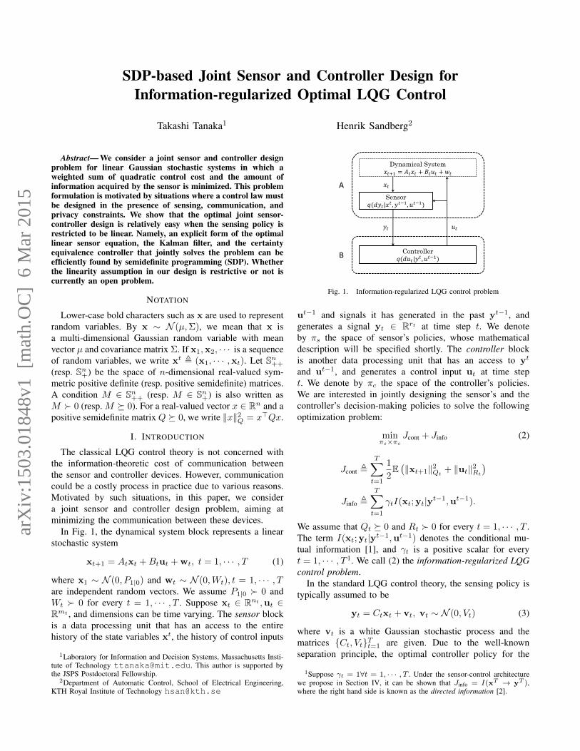
In Fig. 1, the dynamical system block represents a linearstochastic system

xt+1 = Atxt +Btut + wt, t = 1, · · · , T (1)

where x1 ∼ N (0, P1|0) and wt ∼ N (0,Wt), t = 1, · · · , Tare independent random vectors. We assume P1|0 � 0 andWt � 0 for every t = 1, · · · , T . Suppose xt ∈ Rnt ,ut ∈Rmt , and dimensions can be time varying. The sensor blockis a data processing unit that has an access to the entirehistory of the state variables xt, the history of control inputs

1Laboratory for Information and Decision Systems, Massachusetts Insti-tute of Technology ttanaka@mit.edu. This author is supported bythe JSPS Postdoctoral Fellowship.

2Department of Automatic Control, School of Electrical Engineering,KTH Royal Institute of Technology hsan@kth.se

Dynamical System 𝑥𝑡+1 = 𝐴𝑡𝑥𝑡 + 𝐵𝑡𝑢𝑡 +𝑤𝑡

Sensor 𝑞(𝑑𝑦𝑡|𝑥

𝑡 , 𝑦𝑡−1, 𝑢𝑡−1)

Controller 𝑞(𝑑𝑢𝑡|𝑦

𝑡 , 𝑢𝑡−1)

𝑢𝑡 𝑦𝑡

𝑥𝑡 A

B

Fig. 1. Information-regularized LQG control problem

ut−1 and signals it has generated in the past yt−1, andgenerates a signal yt ∈ Rrt at time step t. We denoteby πs the space of sensor’s policies, whose mathematicaldescription will be specified shortly. The controller blockis another data processing unit that has an access to yt

and ut−1, and generates a control input ut at time stept. We denote by πc the space of the controller’s policies.We are interested in jointly designing the sensor’s and thecontroller’s decision-making policies to solve the followingoptimization problem:

minπs×πc

Jcont + Jinfo (2)

Jcont ,T∑t=1

1

2E(‖xt+1‖2Qt

+ ‖ut‖2Rt

)Jinfo ,

T∑t=1

γtI(xt;yt|yt−1,ut−1).

We assume that Qt � 0 and Rt � 0 for every t = 1, · · · , T .The term I(xt;yt|yt−1,ut−1) denotes the conditional mu-tual information [1], and γt is a positive scalar for everyt = 1, · · · , T 1. We call (2) the information-regularized LQGcontrol problem.

In the standard LQG control theory, the sensing policy istypically assumed to be

yt = Ctxt + vt, vt ∼ N (0, Vt) (3)

where vt is a white Gaussian stochastic process and thematrices {Ct, Vt}Tt=1 are given. Due to the well-knownseparation principle, the optimal controller policy for the

1Suppose γt = 1∀t = 1, · · · , T . Under the sensor-control architecturewe propose in Section IV, it can be shown that Jinfo = I(xT → yT ),where the right hand side is known as the directed information [2].

arX

iv:1

503.

0184

8v1

[m

ath.

OC

] 6

Mar

201

5

standard LQG control problem minπcJcont can be found by

solving forward and backward Riccati recursions. In (2),in contrast, we do not assume (3), and allow sensors tobe any causal data collecting mechanism in πs. However,minπs×πc

Jcont is an uninteresting problem, since triviallyyt = xt (perfect observation) together with the linear-quadratic regulator (LQR) is optimal. To exclude this trivialsolution, we aim at minimizing Jcont + Jinfo as in (2), whichamounts to charging the cost γt for every bit of innovativeinformation collected by the sensor at time step t. Noticethat full observation yt = xt results in Jinfo = +∞.

Although we are not aware of a complete solution to (2),we here provide an SDP-based algorithm to construct anoptimal linear sensor-controller joint policy. This result turnsout to be an extension of an SDP-based algorithm for thesequential rate-distortion problem proposed in [3].

II. APPLICATIONS AND RELATED WORK

In this section, we briefly summarize connections betweenthe information-regularized LQG control problem (2) andrelated work in the control, information theory, robotics,social science, and economics literature.

A. Control over a communication channel

In Fig. 1, suppose that agents A and B are geographicallyseparated, and the communication channel from A to B isband-limited. Suppose that agents A and B are in collabora-tion to design the sensor and controller blocks. What kind ofdata should then a sensor collect and transmit, so that B cangenerate a satisfactory control signal in a real-time manner?

Feedback control over noisy channels has been a popularresearch topic in the past two decades. Most of the earlycontributions focus on stabilization of unstable dynamicalsystems using feeback control over band-limited communi-cation channels. A very partial list of papers in this contextis [4]–[10]. This research direction naturally leads to trade-off studies between the achievable control performance andthe required capacity of the sensor-controller communicationchannel. If the communication rate is finite, larger blocklength (achieving high resolution) is not necessarily preferredsince the resulting delay leads to the loss of control perfor-mance [11]. LQG control performance subject to capacityconstraints is considered in [12], where a certain “separationprinciple” between control design and communication designis reported. The authors of [13] consider a fundamental per-formance limitation of the finite horizon minimum-variancecontrol (MVC) over noisy communication channels in theLQG regime. More comprehensive literature surveys oncontrol designs over communication channels are availablein [14]–[17].

However, the majority of the existing work in this con-text assume sensor models and/or channel models a priori,and are different from (2). A few exceptions include [18]and [19], where sensor-controller joint design problems areconsidered. However, these works are concerned with sensorpower constraints rather than information constraints, and aredifferent from (2). Our problem formulation (2) falls into

a general class of sensor optimization problems consideredin [20], where several results are derived regarding theconvexity of the problem and the existence of an optimalsolution under different choices of topologies in the space ofsensors. However, no structural results on specific problemsappear there.

B. Bounded rationality

Broadly, the term bounded rationality is used to referto the limited ability of decision makers (human or robot)to acquire and process information. The rational inatten-tion model introduced by [21] in the economics literaturecharacterizes bounded rationality using the idea of Shan-non’s channel capacity. Inspired by this model, recently[22] considered an information-constrained LQG controlproblem, which is similar to (2). In this paper, we removethe somewhat restrictive assumptions made in [22], includingthat a controller there is a time invariant function of thecurrent state only. Furthermore, our SDP-based approach ispowerful in handling multi-dimensional systems, while [22]is currently restricted to scalar systems.

C. Privacy-preserving control

In Fig. 1, suppose that agent A can privately observeits internal state xt, and that xt must be controlled by anexternal agent B through control input ut. At every timestep, a message yt containing information about the currentstate xt is created by the agent A and is sent to the agentB, so that B can compute desirable control inputs. However,sending yt = xt may not be desirable for a privacy-awareagent A, since this means a complete loss of privacy. Whatis then the optimal message yt?

Suppose that the loss of privacy caused by disclosingyt at time step t is quantified by the conditional mutualinformation I(xt;yt|yt−1,ut−1). Conditioning on yt−1 andut−1 reflects the fact that agent B knows a realizationof these random variables by the time he receives a newmessage yt. (Similar quantities are used to evaluate privacyin wiretap channel problems [23], as well as in more recentdatabase literature [24] [25].) Introducing the “price of pri-vacy” γt, the optimal privacy-preserving control problem canbe formulated as (2). In contrast, [26] employs differentialprivacy as a privacy measure in dynamic state estimationproblems.

III. PROBLEM FORMULATION

A. Information-regularized LQG control problem

In this paper, both the sensor’s and controller’s policies aremodeled by Borel-measurable stochastic kernels. Set X =Rn and Y = Rm and let BX and BY be the Borel σ-algebrason X and Y respectively, with respect to the usual topology.

Definition 1: A Borel-measurable stochastic kernel from(X,BX ) to (Y,BY) is a map q(·|·) : BY×X→ [0, 1] such that• q(·|x) is a probability measure on (Y,BY) for every x∈X .• q(E|·) is BX -measurable for every E ∈ BY .

A Borel-measurable stochastic kernel from (X ,BX ) to(Y,BY) will be simply referred to as a stochastic kernel fromX to Y , and denoted by q(dy|x). The space of stochastickernels from X to Y is denoted by Qy|x.

The sensor’s policy at time t is a stochastic kernel fromX t×Yt−1×U t−1 to Yt. The controller’s policy at time t isa stochastic kernel from Yt×U t−1 to Ut. Using the notationabove, the policy spaces πs and πc are formally defined by

πs =

T∏t=1

Qyt|xt,yt−1,ut−1 and πc =

T∏t=1

Qut|yt,ut−1 .

Then, (2) is an optimization problem over the sequencesof stochastic kernels {q(dyt|xt, yt−1, ut−1)}Tt=1 ∈ πs and{q(dut|yt, ut−1)}Tt=1 ∈ πc. Once an element in πs × πc ispicked, then a joint probability measure p(dxT , dyT , duT )over X T × YT × ZT is uniquely determined (see Proposi-tion 7.28 in [27]).

B. Restricted problem

To the best of the authors’ knowledge, little is knownabout the structure of the optimal solution to (2). Namely,it is currently unknown whether there exists a jointly linearpolicy in πs × πc that attains optimality in (2)2. Hence, inthis paper, we focus on a restricted problem in which sensor’spolicy is restricted to the form (3). That is, we consider

minπlins ×πc

Jcont + Jinfo (4)

where πlins is the space of sequences of stochastic kernels

{q(dyt|xt)}Tt=1, which can be realized by a linear sensorequation (3) with some Ct and Vt to be determined. Wetackle this problem by applying an SDP-based solution tothe sequential rate-distortion (SRD) problem obtained in [3].Based on the existence of a linear optimal solution to theGaussian SRD problem (as shown in [28]), we will showthat (4) has a jointly linear optimal solution.

IV. SUMMARY OF THE RESULT

In this section, we provide a complete solution to therestricted information-regularized LQG control problem (4).Specifically, we claim that the following numerical procedureallows us to explicitly construct the optimal stochastic ker-nels {q(dyt|xt)}Tt=1 ∈ πlin

s and {q(dut|yt, ut−1)}Tt=1 ∈ πcfor (4).

Step 1. (Controller design) Compute a backward Riccatirecursion.

St =

{Qt if t = T

Qt +Nt+1 if t = 1, · · · , T − 1(5a)

Mt = B>t StBt +Rt (5b)

Nt = A>t (St − StBtM−1t B>t St)At (5c)

Kt = −M−1t B>t StAt (5d)

Θt = K>t MtKt (5e)

2Our problem is different from the optimal LQG control over Gaussianchannels, where a linear encoder-controller pair is optimal (e.g., [17] Ch.11).

The matrix St is commonly understood in the LQR theoryas the “cost-to-go” function, while Kt is the optimal controlgain. The auxiliary parameter Θt will be used in Step 2.

Step 2. (Covariance scheduling) Solve a max-det problemwith respect to {Pt|t,Πt}Tt=1 subject to the LMI constraints:

min

T∑t=1

(1

2Tr(ΘtPt|t)−

γt2

log det Πt

)+ C (6a)

s.t. Πt � 0, t = 1, · · · , T (6b)

Pt+1|t+1 � AtPt|tA>t +Wt, t=1, · · ·, T−1 (6c)P1|1 � P1|0, PT |T = ΠT (6d)[Pt|t−Πt Pt|tA

>t

AtPt|t Wt+AtPt|tA>t

]�0, t=1, · · ·, T−1 (6e)

where C is a constant3. Due to the boundedness of thefeasible set, (6) has an optimal solution4.

Step 3. (Sensor design) Set rt = rank(P−1t|t − P−1t|t−1) for

every t = 1, · · · , T , where

Pt|t−1 , At−1Pt−1|t−1A>t−1 +Wt−1, t = 2, · · · , T.

Choose matrices Ct ∈ Rrt×nt and Vt ∈ Srt++ so that theysatisfy

C>t V−1t Ct = P−1t|t − P

−1t|t−1 (7)

for t = 1, · · · , T . For instance, the singular value decompo-sition can be used. In particular, in case of rt = 0, Ct andVt are considered to be null (zero dimensional) matrices.

Step 4. (Filter design) Determine the Kalman gains by

Lt = Pt|t−1C>t (CtPt|t−1C

>t + Vt)

−1. (8)

If rt = 0, Lt is a null matrix.Step 5. (Policy construction) Using {Ct, Vt, Lt,Kt}Tt=1

obtained above, define the sensor’s policy {q(dyt|xt)}Tt=1 ∈πlins by equation (3). When rt = 0, the optimal dimension

of the sensing vector yt is zero, meaning that no sensing isthe optimal strategy. On the other hand, define a controller’spolicy {q(dut|yt, ut−1)}Tt=1 ∈ πc by the certainty equiva-lence controller ut = Ktxt where xt = E(xt|yt,ut−1) isobtained by the standard Kalman filter

xt = xt|t−1 + Lt(yt − Ctxt|t−1) (9a)xt+1|t = Atxt +Btut. (9b)

When rt = 0, (9a) is simply replaced by xt = xt|t−1.

3 The constant is given by

C =

T−1∑t=1

(γtnt

2log

γt+1

γt+γt

2log detWt

)+γ1

2log detP1|0

+1

2Tr(N1P1|0) +

1

2

T∑t=1

Tr(WtSt).

4One can replace (6b) with Πt � εI without altering the result. Thisconversion makes the feasible set compact and thus the Weierstrass theoremcan be used.

Theorem 1: There exists a joint sensor-controller policyin πlin

s × πc that attains optimality in (4). The optimalvalue of (4) coincides with the optimal value of the max-det problem (6). Furthermore, an optimal policy can beconstructed by the Steps 1-5.

V. DERIVATION OF THE MAIN RESULT

We first show that, once the sensor’s policy {qyt|xt}Tt=1 ∈

πlins is fixed, then Jinfo does not depend on the choice of

controller’s policy. This observation allows us to rewrite (2)as

minπlins

(Jinfo + min

πc

Jcont

). (10)

Then, we interpret (10) as a two-player Stackelberg game(see, e.g., [29]) in which the sensor agent (agent A in Fig. 1)is the leader and the controller agent (agent B) is the follower.If the sensor’s policy is given, the controller’s best responsecan be explicitly found by solving a stochastic optimalcontrol problem minπc

Jcont. With an explicit expression ofminπc

Jcont, we show that the outer optimization problem in(10) over πlin

s becomes the sequential rate-distortion problem[28], whose optimal solution can be constructed by solvingan SDP problem [3].

Fix a joint sensor-controller policy in πlins × πc and let

p(dxT , dyT , duT ) be the resulting joint probability mea-sure. Let p(dxt|yt−1, ut−1) and p(dxt|yt, ut−1) be proba-bility measures obtained by conditioning and marginalizingp(dxT , dyT , duT ). It follows from the standard Kalmanfiltering theory that

p(dxt|yt−1, ut−1) ∼ N (xt|t−1, Pt|t−1)

p(dxt|yt, ut−1) ∼ N (xt, Pt|t)

where {Pt|t} and {Pt|t−1} satisfy

Pt|t−1 = At−1Pt−1|t−1A>t−1 +Wt−1 (11a)

Pt|t = (P−1t|t−1 + C>t V−1t Ct)

−1, (11b)

while xt and xt|t−1 are recursively obtained by (9). Usingmatrices {Pt|t} and {Pt|t−1}, the mutual information termscan be explicitly written as

I(xt;yt|yt−1,ut−1) = h(xt|yt−1,ut−1)− h(xt|yt,ut−1)

=1

2log detPt|t−1−

1

2log detPt|t.

Therefore,

Jinfo ,T∑t=1

γtI(xt;yt|yt−1,ut−1)

=

T−1∑t=1

(γt+1

2log detPt+1|t −

γt2

log detPt|t

)+γ12

log detP1|0 −γT2

log detPT |T .

In particular, this result clearly shows that the mutualinformation terms are control-independent, since they arecompletely determined by (11) once the sequence of matrices

{Ct, Vt}Tt=1 is fixed. This observation justifies the equiva-lence between (4) and (10).

Next, let us focus on the stochastic optimal control prob-lem minπc

Jcont, whose solution is well understood.Lemma 1: For every fixed {qyt|xt

}Tt=1 ∈ πlins , the cer-

tainty equivalence controller ut = Ktxt where xt =E(xt|yt,ut−1) is an optimizer of minπc

Jcont. Moreover,

minπc

Jcont =1

2Tr(N1P1|0)+

1

2

T∑k=1

(Tr(WkSk)+Tr(ΘkPk|k)

).

Proof: This is a standard result and can be shown bydynamic programming. A proof is provided in Appendix.

Combining the results so far, we have shown that

Jinfo + minπc

Jcont

=

T−1∑t=1

(1

2Tr(ΘtPt|t)+

γt+1

2log detPt+1|t−

γt2

log detPt|t

)+

1

2Tr(ΘTPT |T )− γT

2log detPT |T + c (12)

where c= 12Tr(N1P1|0) + γ1

2 log detP1|0 + 12

∑Tt=1Tr(WtSt)

is a constant. The expression (12) is the cost of the originalproblem (2) when the sensor model {Ct, Vt}Tt=1 is fixedand the controller agent (Stackelberg follower) reacts withthe best response. Notice that (12) is a function of thesequence {Ct, Vt}Tt=1, since the matrices Pt|t and Pt+1|t aredetermined by (11).

Now we have formulated a problem for the sensor agent(Stackelberg leader). Namely, the sensor agent needs to findthe optimal sequence of matrices {Ct, Vt}Tt=1 (as well astheir dimensions) that minimizes (12). Next, we show thatthis can be done very efficiently by solving a semidefiniteprogramming problem.

Let us first focus on the quantityγt+1

2log detPt+1|t −

γt2

log detPt|t. (13)

Introducing At =√

γt+1

γtAt and Wt = γt+1

γtWt,

2

γt× (13) = log det(AtPt|tA

>t + Wt)− log detPt|t

= log det Wt − log det(P−1t|t +A>t W−1t At)

−1 (14a)

= min log detWt−log det Πt+nt log

(γt+1

γt

)(14b)

s.t. 0 ≺ Πt � (P−1t|t +A>t W−1t At)

−1

= min log detWt−log det Πt+nt log

(γt+1

γt

)(14c)

s.t.[Pt|t−Πt Pt|tA

>t

AtPt|t AtPt|tA>t +Wt

]� 0,Πt � 0

We have used Sylvester’s determinant theorem in step (14a).The quantity (14a) is equal to the optimal value of a con-strained optimization problem (14b) with decision variablesPt|t and Πt, and this rewriting is possible because of themonotonicity of the determinant function. In (14c), the

Ω

+𝑋

+𝑌

+𝑍

𝜓

𝜙

𝜃

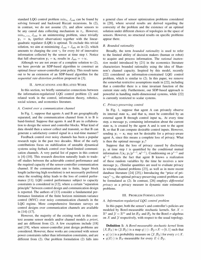
Fig. 2. Orbital coordinate and desired attitude of a nadir-pointing satellite.

constraint Πt � (P−1t|t + A>t W−1t At)

−1 is rewritten usingthe Schur complement formula. The final expression (14c)is particularly useful, since this is a max-det problem subjectto linear matrix inequality (LMI) constraints.

Applying the discussion above to every t = 1, · · · , T − 1,and introducing ΠT = PT |T for notational convenience, itfollows from (12) that the optimal J is equal to the valueof the following optimization problem with respect to thedecision variables {Pt|t,Πt, Ct, Vt}Tt=1:

min

T∑t=1

(1

2Tr(ΘtPt|t)−

γt2

log det Πt

)+ C

s.t.[Pt|t−Πt Pt|tA

>t

AtPt|t AtPt|tA>t +Wt

]� 0, t=1, · · ·, T−1

Πt � 0, t = 1, · · ·TΠT = PT |T

P−11|1 = P−11|0 + C>1 V−11 C1

P−1t|t =(At−1Pt−1|t−1A>t−1 +Wt)

−1+ C>t V−1t Ct

t = 2, · · · , T.

The last two constraints are obtained by eliminating Pt|t−1from (11). These equality constraints themselves are difficultto handle, but can be replaced by the inequality constraints

0 ≺ P1|1 � P1|0

0 ≺ Pt|t � At−1Pt−1|t−1A>t−1 +Wt−1.

These replacements eliminate the variables {Ct, Vt}Tt=1, andconvert the above optimization problem into an alternativeproblem with respect to {Pt|t,Πt}Tt=1 only, as shown in(6). The eliminated variables {Ct, Vt}Tt=1 can be easilyreconstructed by (7).

Solving (6) allows us to optimally schedule the sequenceof covariance matrices. The optimal covariance sequence canbe attained by the Kalman filter (9).

VI. EXAMPLE

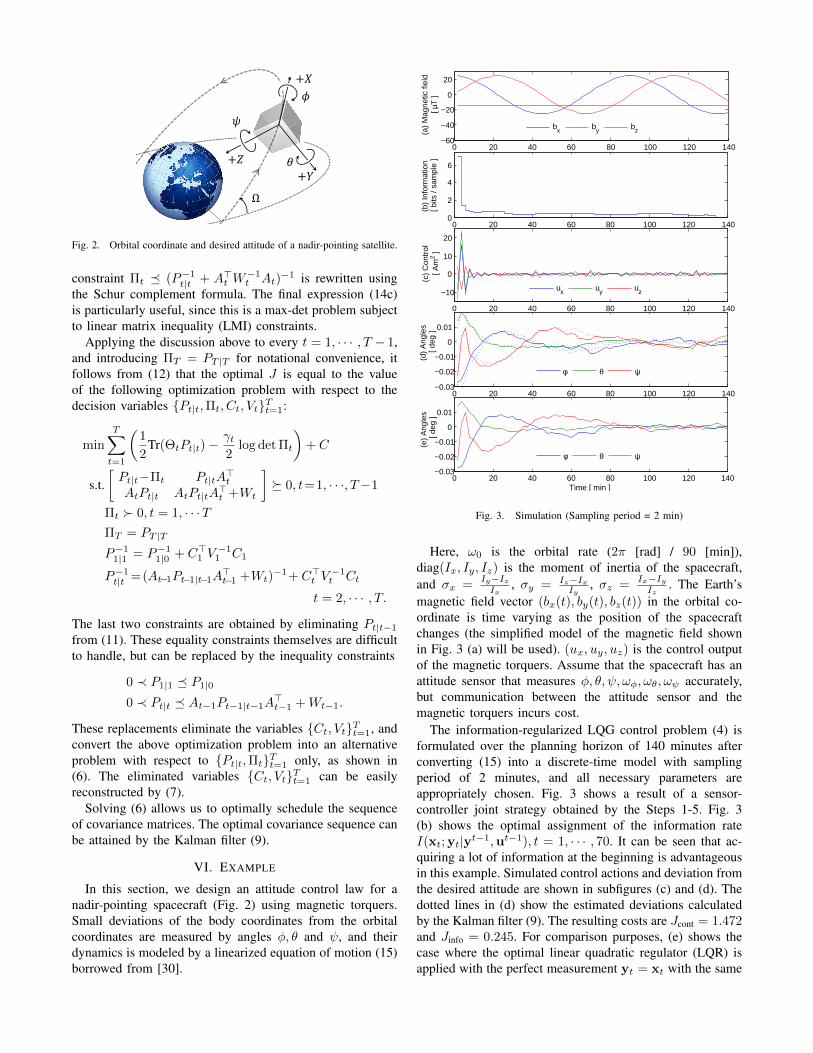
In this section, we design an attitude control law for anadir-pointing spacecraft (Fig. 2) using magnetic torquers.Small deviations of the body coordinates from the orbitalcoordinates are measured by angles φ, θ and ψ, and theirdynamics is modeled by a linearized equation of motion (15)borrowed from [30].

0 20 40 60 80 100 120 140−60

−40

−20

0

20

(a)

Mag

netic

fiel

d [

µT ]

0 20 40 60 80 100 120 1400

2

4

6

(b)

Info

rmat

ion

[ bits

/ sa

mpl

e ]

0 20 40 60 80 100 120 140

−10

0

10

20

(c)

Con

trol

[ A

m2 ]

0 20 40 60 80 100 120 140−0.03

−0.02

−0.01

0

0.01

(d)

Ang

les

[ de

g ]

0 20 40 60 80 100 120 140−0.03

−0.02

−0.01

0

0.01(e

) A

ngle

s [

deg

]

Time [ min ]

bx by bz

ux uy uz

φ θ ψ

φ θ ψ

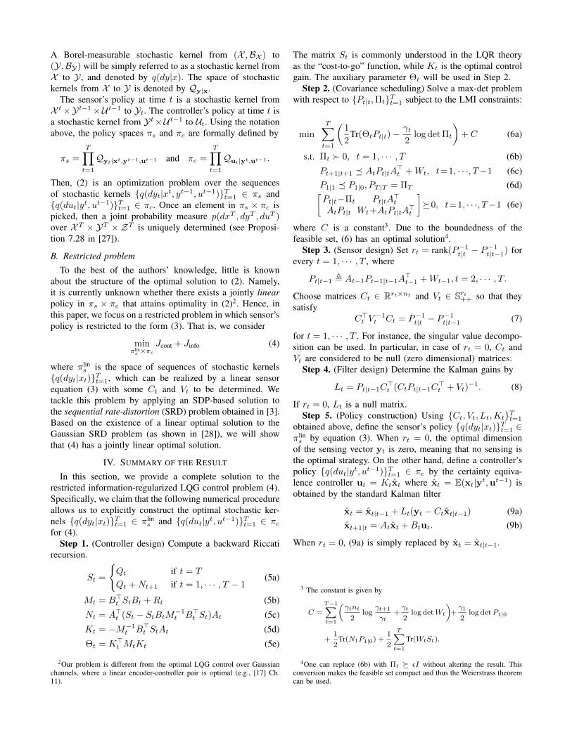
Fig. 3. Simulation (Sampling period = 2 min)

Here, ω0 is the orbital rate (2π [rad] / 90 [min]),diag(Ix, Iy, Iz) is the moment of inertia of the spacecraft,and σx =

Iy−IzIx

, σy = Iz−IxIy

, σz =Ix−IyIz

. The Earth’smagnetic field vector (bx(t), by(t), bz(t)) in the orbital co-ordinate is time varying as the position of the spacecraftchanges (the simplified model of the magnetic field shownin Fig. 3 (a) will be used). (ux, uy, uz) is the control outputof the magnetic torquers. Assume that the spacecraft has anattitude sensor that measures φ, θ, ψ, ωφ, ωθ, ωψ accurately,but communication between the attitude sensor and themagnetic torquers incurs cost.

The information-regularized LQG control problem (4) isformulated over the planning horizon of 140 minutes afterconverting (15) into a discrete-time model with samplingperiod of 2 minutes, and all necessary parameters areappropriately chosen. Fig. 3 shows a result of a sensor-controller joint strategy obtained by the Steps 1-5. Fig. 3(b) shows the optimal assignment of the information rateI(xt;yt|yt−1,ut−1), t = 1, · · · , 70. It can be seen that ac-quiring a lot of information at the beginning is advantageousin this example. Simulated control actions and deviation fromthe desired attitude are shown in subfigures (c) and (d). Thedotted lines in (d) show the estimated deviations calculatedby the Kalman filter (9). The resulting costs are Jcont = 1.472and Jinfo = 0.245. For comparison purposes, (e) shows thecase where the optimal linear quadratic regulator (LQR) isapplied with the perfect measurement yt = xt with the same

φ

θ

ψωφωθωψ

=

0 0 0 1 0 00 0 0 0 1 00 0 0 0 0 1

−4ω20σx 0 0 0 0 ω0(1−σx)

0 3ω20σy 0 0 0 0

0 0 ω20σz −ω0(1+σz) 0 1

φθψωφωθωψ

+

0 0 00 0 00 0 00 bz(t)/Ix −by(t)/Ix

−bz(t)/Iy 0 bx(t)/Iyby(t)/Iz −bx(t)/Iz 0

uxuyuz

+wφwθwψnφnθnψ

(15)

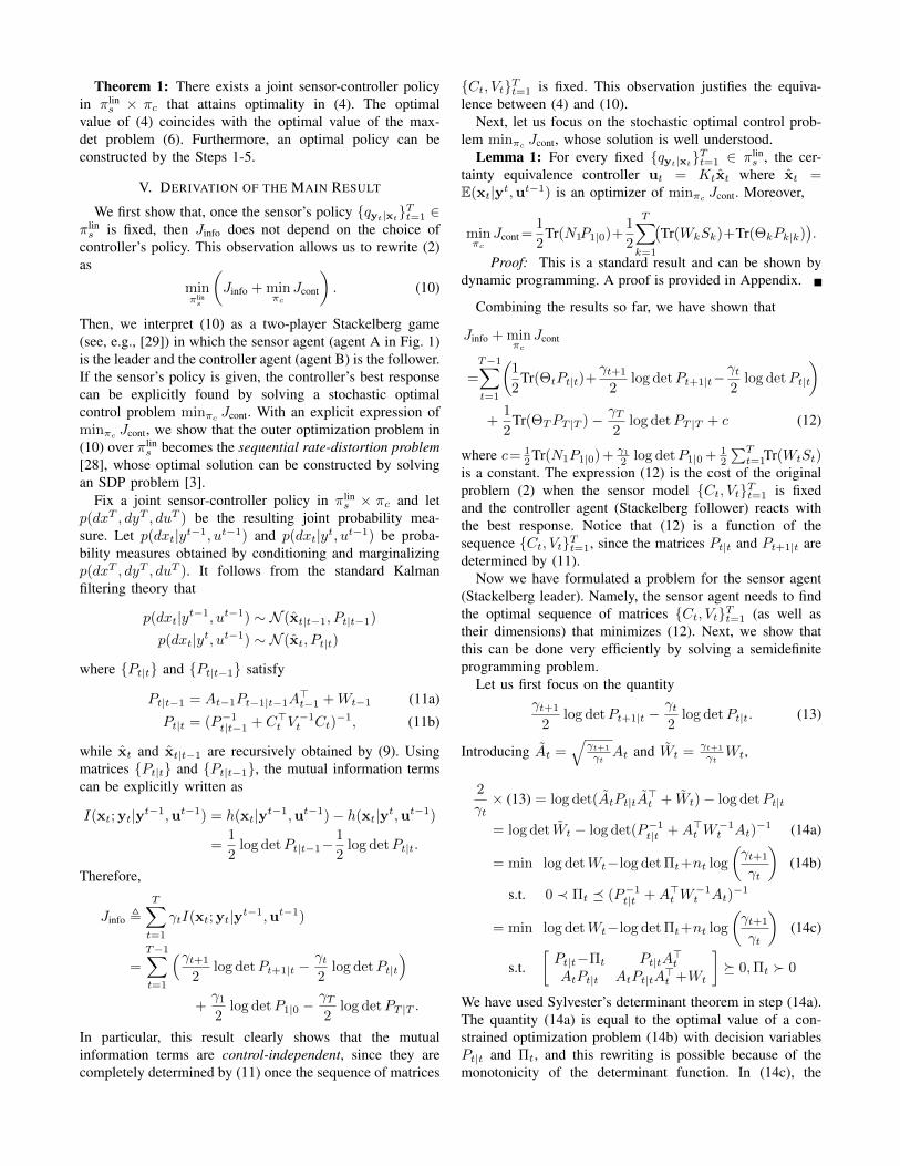
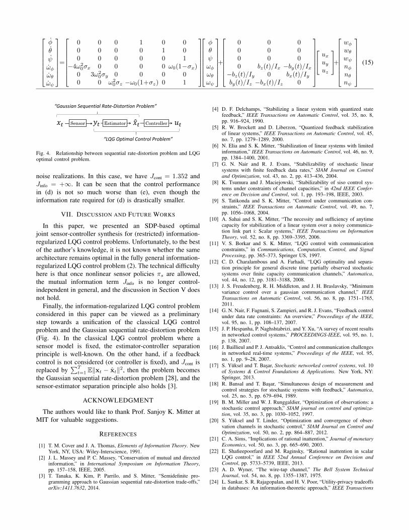
𝑥𝑡 𝑦𝑡 𝑢𝑡 𝑥 𝑡 Sensor Estimator Controller

“Gaussian Sequential Rate-Distortion Problem”

“LQG Optimal Control Problem”

Fig. 4. Relationship between sequential rate-distortion problem and LQGoptimal control problem.

noise realizations. In this case, we have Jcont = 1.352 andJinfo = +∞. It can be seen that the control performancein (d) is not so much worse than (e), even though theinformation rate required for (d) is drastically smaller.

VII. DISCUSSION AND FUTURE WORKS

In this paper, we presented an SDP-based optimaljoint sensor-controller synthesis for (restricted) information-regularized LQG control problems. Unfortunately, to the bestof the author’s knowledge, it is not known whether the samearchitecture remains optimal in the fully general information-regularized LQG control problem (2). The technical difficultyhere is that once nonlinear sensor policies πs are allowed,the mutual information term Jinfo is no longer control-independent in general, and the discussion in Section V doesnot hold.

Finally, the information-regularized LQG control problemconsidered in this paper can be viewed as a preliminarystep towards a unification of the classical LQG controlproblem and the Gaussian sequential rate-distortion problem(Fig. 4). In the classical LQG control problem where asensor model is fixed, the estimator-controller separationprinciple is well-known. On the other hand, if a feedbackcontrol is not considered (or controller is fixed), and Jcont isreplaced by

∑Tt=1 E‖xt − xt‖2, then the problem becomes

the Gaussian sequential rate-distortion problem [28], and thesensor-estimator separation principle also holds [3].

ACKNOWLEDGMENT

The authors would like to thank Prof. Sanjoy K. Mitter atMIT for valuable suggestions.

REFERENCES

[1] T. M. Cover and J. A. Thomas, Elements of Information Theory. NewYork, NY, USA: Wiley-Interscience, 1991.

[2] J. L. Massey and P. C. Massey, “Conservation of mutual and directedinformation,” in International Symposium on Information Theory,pp. 157–158, IEEE, 2005.

[3] T. Tanaka, K. Kim, P. Parrilo, and S. Mitter, “Semidefinite pro-gramming approach to Gaussian sequential rate-distortion trade-offs,”arXiv:1411.7632, 2014.

[4] D. F. Delchamps, “Stabilizing a linear system with quantized statefeedback,” IEEE Transactions on Automatic Control, vol. 35, no. 8,pp. 916–924, 1990.

[5] R. W. Brockett and D. Liberzon, “Quantized feedback stabilizationof linear systems,” IEEE Transactions on Automatic Control, vol. 45,no. 7, pp. 1279–1289, 2000.

[6] N. Elia and S. K. Mitter, “Stabilization of linear systems with limitedinformation,” IEEE Transactions on Automatic Control, vol. 46, no. 9,pp. 1384–1400, 2001.

[7] G. N. Nair and R. J. Evans, “Stabilizability of stochastic linearsystems with finite feedback data rates,” SIAM Journal on Controland Optimization, vol. 43, no. 2, pp. 413–436, 2004.

[8] K. Tsumura and J. Maciejowski, “Stabilizability of siso control sys-tems under constraints of channel capacities,” in 42nd IEEE Confer-ence on Decision and Control, vol. 1, pp. 193–198, IEEE, 2003.

[9] S. Tatikonda and S. K. Mitter, “Control under communication con-straints,” IEEE Transactions on Automatic Control, vol. 49, no. 7,pp. 1056–1068, 2004.

[10] A. Sahai and S. K. Mitter, “The necessity and sufficiency of anytimecapacity for stabilization of a linear system over a noisy communica-tion link part i: Scalar systems,” IEEE Transactions on InformationTheory, vol. 52, no. 8, pp. 3369–3395, 2006.

[11] V. S. Borkar and S. K. Mitter, “LQG control with communicationconstraints,” in Communications, Computation, Control, and SignalProcessing, pp. 365–373, Springer US, 1997.

[12] C. D. Charalambous and A. Farhadi, “LQG optimality and separa-tion principle for general discrete time partially observed stochasticsystems over finite capacity communication channels,” Automatica,vol. 44, no. 12, pp. 3181–3188, 2008.

[13] J. S. Freudenberg, R. H. Middleton, and J. H. Braslavsky, “Minimumvariance control over a gaussian communication channel,” IEEETransactions on Automatic Control, vol. 56, no. 8, pp. 1751–1765,2011.

[14] G. N. Nair, F. Fagnani, S. Zampieri, and R. J. Evans, “Feedback controlunder data rate constraints: An overview,” Proceedings of the IEEE,vol. 95, no. 1, pp. 108–137, 2007.

[15] J. P. Hespanha, P. Naghshtabrizi, and Y. Xu, “A survey of recent resultsin networked control systems,” PROCEEDINGS-IEEE, vol. 95, no. 1,p. 138, 2007.

[16] J. Baillieul and P. J. Antsaklis, “Control and communication challengesin networked real-time systems,” Proceedings of the IEEE, vol. 95,no. 1, pp. 9–28, 2007.

[17] S. Yuksel and T. Basar, Stochastic networked control systems, vol. 10of Systems & Control Foundations & Applications. New York, NY:Springer, 2013.

[18] R. Bansal and T. Basar, “Simultaneous design of measurement andcontrol strategies for stochastic systems with feedback,” Automatica,vol. 25, no. 5, pp. 679–694, 1989.

[19] B. M. Miller and W. J. Runggaldier, “Optimization of observations: astochastic control approach,” SIAM journal on control and optimiza-tion, vol. 35, no. 3, pp. 1030–1052, 1997.

[20] S. Yuksel and T. Linder, “Optimization and convergence of obser-vation channels in stochastic control,” SIAM Journal on Control andOptimization, vol. 50, no. 2, pp. 864–887, 2012.

[21] C. A. Sims, “Implications of rational inattention,” Journal of monetaryEconomics, vol. 50, no. 3, pp. 665–690, 2003.

[22] E. Shafieepoorfard and M. Raginsky, “Rational inattention in scalarLQG control,” in IEEE 52nd Annual Conference on Decision andControl, pp. 5733–5739, IEEE, 2013.

[23] A. D. Wyner, “The wire-tap channel,” The Bell System TechnicalJournal, vol. 54, no. 8, pp. 1355–1387, 1975.

[24] L. Sankar, S. R. Rajagopalan, and H. V. Poor, “Utility-privacy tradeoffsin databases: An information-theoretic approach,” IEEE Transactions

on Information Forensics and Security, vol. 8, no. 6, pp. 838–852,2013.

[25] A. Makhdoumi, S. Salamatian, N. Fawaz, and M. Medard, “From theinformation bottleneck to the privacy funnel,” arXiv:1402.1774, 2014.

[26] J. Le Ny and G. J. Pappas, “Differentially private filtering,” AutomaticControl, IEEE Transactions on, vol. 59, no. 2, pp. 341–354, 2014.

[27] D. P. Bertsekas and S. E. Shreve, Stochastic optimal control: Thediscrete time case, vol. 139. Academic Press New York, 1978.

[28] S. Tatikonda, “Control under communication constraints,” PhD thesis,Massachusetts Institute of Technology, 2000.

[29] T. Basar and G. J. Olsder, Dynamic Noncooperative Game Theory.Classics in Applied Mathematics, Society for Industrial and AppliedMathematics, 1999.

[30] M. L. Psiaki, “Magnetic torquer attitude control via asymptotic peri-odic linear quadratic regulation,” Journal of Guidance, Control, andDynamics, vol. 24, no. 2, pp. 386–394, 2001.

APPENDIX

We consider minπc Jcont as a T -stage dynamic program-ming problem. The state of the system at stage t is a jointprobability measure p(dxt, dyt, dut−1) which is updated by

p(dxt+1, dyt+1, dut) =q(dyt+1|xt+1)f(dxt+1|xt, ut)× q(dut|yt, ut−1)p(dxt, dyt, dut−1).

Here, the stochastic kernel f(dxt+1|xt, ut) is given by(1), while q(dyt+1|xt+1) is the sensing policy, which isassumed to be fixed. The stochastic kernel q(dut|yt, ut−1) ∈Qut|yt,ut−1 is the control variable in this dynamic program-ming formulation. The associated Bellman’s equation is

Jt(p(dxt, dyt, dut−1)) =

minQut|yt,ut−1

{1

2E(‖xt+1‖2Qt

+‖ut‖2Rt

)+Jt+1(p(dxt+1, dyt+1, dut))

}with the boundary condition JT+1(·) = 0.

Claim 1: For every t = 1, · · · , T , the certainty equiva-lence controller ut = Ktxt where x , E(xt|yt,ut−1) is theoptimal control policy in Qut|yt,ut−1 . Moreover, for everyt = 1, · · · , T ,

Jt(qxt,yt,ut−1) =

1

2E‖xt‖2Nt

+1

2

T∑k=t

(Tr(WkSk)+Tr(ΘkPk|k)

). (16)

Proof: Equation (16) holds when t = T as

JT (qxT ,yT ,uT−1)

= minQuT |yT,uT−1

1

2E(‖AtxT +BtuT +wT ‖2QT

+‖uT ‖2RT

)= minQuT |yT,uT−1

1

2E(‖xT ‖2NT

+‖wT ‖2QT+‖uT−KTxT ‖2MT

)=

1

2E‖xT ‖2NT

+1

2

(Tr(WTQT ) + Tr(ΘTPT |T )

).

Notice that in the second expression, uT appears onlyin ‖uT −KTxT ‖2MT

. By choosing uT = KTE(xT |yT ),this quantity attains its minimum value E‖KT (x −E(xT |yT ))‖2MT

= Tr(ΘTPT |T ). So assume (16) holds for

t = l + 1. Then

Jl(qxl,yl,ul−1)

= minQuT |yT,uT−1

{1

2E(‖xl+1‖2Ql

+‖ul‖2Rl

)+

1

2E‖xl+1‖2Nl+1

+1

2

T∑k=l+1

(Tr(WkSk)+Tr(ΘkPk|k)

)}

= minQuT |yT,uT−1

{1

2E(‖xl+1‖2Sl

+‖ul‖2Rl

)+

1

2

T∑k=l+1

(Tr(WkSk)+Tr(ΘkPk|k)

)}

=1

2

T∑k=l+1

(Tr(WkSk)+Tr(ΘkPk|k)

)+ minQ

ul|yl,ul−1

1

2E(‖Alxl +Blul + wl‖2Sl

+ ‖ul‖2Rl

)=

1

2

T∑k=l+1

(Tr(WkSk)+Tr(ΘkPk|k)

)+

1

2E‖xl‖2Nl

+1

2

(Tr(WlSl)+Tr(ΘlPl|l)

)=

1

2E‖xl‖2Nl

+1

2

T∑k=l

(Tr(WkSk) + Tr(ΘkPk|k)

).

Noticing E‖x1‖2N1= Tr(N1P1|0), Lemma 1 follows from

Claim 1.