SDPT3 — a Matlab software package forsemidefinite-quadratic-linear programming,

version 3.0

R. H. Tutuncu ∗, K. C. Toh †, and M. J. Todd ‡.

August 21, 2001

Abstract

This document describes a new release, version 3.0, of the software SDPT3. Thiscode is designed to solve conic programming problems whose constraint cone is aproduct of semidefinite cones, second-order cones, and/or nonnegative orthants. Itemploys a predictor-corrector primal-dual path-following method, with either theHKM or the NT search direction. The basic code is written in Matlab, but keysubroutines in Fortran and C are incorporated via Mex files. Routines are providedto read in problems in either SeDuMi or SDPA format. Sparsity and block diagonalstructure are exploited, but the latter needs to be given explicitly.

∗Department of Mathematical Sciences, Carnegie Mellon University, Pittsburgh, PA 15213, USA(reha+@andrew.cmu.edu). Research supported in part by NSF through grant CCR-9875559.†Department of Mathematics, National University of Singapore, 10 Kent Ridge Crescent, Singapore

119260. (mattohkc@math.nus.edu.sg). Research supported in part by the Singapore-MIT Alliance.‡School of Operations Research and Industrial Engineering, Cornell University, Ithaca, New York 14853,

USA (miketodd@cs.cornell.edu). Research supported in part by NSF through grant DMS-9805602 andONR through grant N00014-96-1-0050.

1

1 Introduction

The current version of SDPT3, version 3.0, can solve conic linear optimization prob-lems with inclusion constraints for the cone of positive semidefinite matrices, thesecond-order cone, and/or the polyhedral cone of nonnegative vectors. It solves thefollowing standard form of such problems, henceforth called SQLP problems:

(P ) min∑nsj=1〈csj , xsj〉 +

∑nqi=1〈c

qi , x

qi 〉 + 〈cl, xl〉

s.t.∑nsj=1(Asj)

T svec(xsj) +∑nqi=1(Aqi )

Txqi + (Al)Txl = b,

xsj ∈ Ksjs ∀j, xqi ∈ Kqi

q ∀i, xl ∈ Knll .

Here, csj , xsj are symmetric matrices of dimension sj and K

sjs is the cone of positive

semidefinite symmetric matrices of the same dimension. Similarly, cqi , xqi are vectors

in IRqi and Kqiq is the second-order cone defined by Kqi

q := {x ∈ IRqi : x1 ≥ ‖x2:qi‖}.Finally, cl, xl are vectors of dimension nl and Knl

l is the cone IRnl+ . In the notationabove, Asj denotes the sj×mmatrix with sj = sj(sj+1)/2 whose columns are obtainedusing the svec operator from m symmetric sj × sj constraint matrices correspondingto the jth semidefinite block xsj . For a definition of the vectorization operator svecon symmetric matrices, see, e.g., [15]. The matrices Aqi ’s are qi × m dimensionalconstraint matrices corresponding to the ith quadratic block xqi , and Al is the l ×mdimensional constraint matrix corresponding to the linear block xl. The notation〈p, q〉 denotes the standard inner product in the appropriate space.

The software also solves the dual problem associated with the problem above:

(D) max bT ys.t. Asjy + zsj = csj , j = 1 . . . , ns

Aqi y + zqi = cqi , i = 1 . . . , nq

Aly + zl = cl,

zsj ∈ Ksjs ∀j, zqi ∈ Kqi

q ∀i, zl ∈ Knll .

This package is written in Matlab version 5.3 and is compatible with Matlab

version 6.0. It is available from the internet sites:

http://www.math.nus.edu.sg/~mattohkc/index.html

http://www.math.cmu.edu/~reha/sdpt3.html

The software package was originally developed to provide researchers in semidef-inite programming with a collection of reasonably efficient and robust algorithmsthat could solve general SDPs with matrices of dimensions of the order of a hun-dred. The current release, version 3.0, expands the family of problems solvable bythe software in two dimensions. First, this version is much faster than the previousrelease [18], especially on large sparse problems, and consequently can solve muchlarger problems. Second, the current release can also directly solve problems that

2

have second-order cone constraints — with the previous version it was necessary toconvert such constraints to semidefinite cone constraints.

In this paper, the vector 2-norm and Frobenius norm are denoted by ‖·‖ and ‖·‖F ,respectively. In the next section, we discuss the algorithm used in the software andseveral implementation details including the initial iterates generated by our softwareand its data storage scheme. Section 3 describes the search directions used by ouralgorithms and explains how they are computed. In Section 4, we provide sample runsand comment on several major differences between the current and earlier versions ofour software. In the last section, we present performance results of our software onproblems from the SDPLIB and DIMACS libraries.

2 A primal-dual infeasible-interior-point algo-

rithm

The algorithm implemented in SDPT3 is a primal-dual interior-point algorithm thatuses the path-following paradigm. In each iteration, we first compute a predictorsearch direction aimed at decreasing the duality gap as much as possible. Afterthat, the algorithm generates a Mehrotra-type corrector step [10] with the intentionof keeping the iterates close to the central path. However, we do not impose anyneighborhood restrictions on our iterates.1 Initial iterates need not be feasible —the algorithm tries to achieve feasibility and optimality of its iterates simultaneously.It should be noted that in our implementation, the user has the option to use aprimal-dual path-following algorithm that does not use corrector steps.

Following next is a pseudo-code for the algorithm we implemented. Note thatthis description makes references to later sections where details related to the algo-rithm are explained.

Algorithm IPC. Suppose we are given an initial iterate (x0, y0, z0) with x0, z0 strictlysatisfying all the conic constraints. Decide on the type of search direction to use. Set γ0 = 0.9.Choose a value for the parameter expon used in e.

For k = 0, 1, . . .

(Let the current and the next iterate be (x, y, z) and (x+, y+, z+) respectively. Also, let thecurrent and the next step-length parameter be denoted by γ and γ+ respectively.)

• Set µ = 〈x, z〉/n, and

rel gap =〈x, z〉

max(1, (|〈c, x〉|+ |bT y|)/2, infeas meas = max

(‖rp‖

max(1, ‖b‖),

‖Rd‖max(1, ‖c‖)

). (1)

Stop the iteration if the infeasibility measure infeas meas and the relative duality gap(rel gap) are sufficiently small.

1This strategy works well on most of the problems we tested. However, it should be noted that theoccasional failure of the software on problems with poorly chosen initial iterates is likely due to the lack ofa neighborhood enforcement in the algorithm.

3

• (Predictor step)Solve the linear system (9) with σ = 0 in the right-side vector (11). Denote the solutionof (3) by (δx, δy, δz). Let αp and βp be the step-lengths defined as in (29) and (30) with∆x,∆z replaced by δx, δz, respectively.

• Take σ to be

σ = min(

1,[〈x+ αp δx, z + βp δz〉

〈x, z〉

]e),

where the exponent e is chosen as follows:

e =

{max[expon, 3 min(αp, βp)2] if µ > 10−6,expon if µ ≤ 10−6.

• (Corrector step)Solve the linear system (9) with Rc in the the right-hand side vector (11) replaced by

Rsc = svec [σµI −HP (smat(xs)smat(zs))−HP (smat(δxs)smat(δzs))]

Rqc = σµeq − TG(xq, zq)− TG(δxq, δzq)

Rlc = σµel − diag(xl)zl − diag(δxl)δzl.

Denote the solution of (3) by (∆x,∆y,∆z).

• Update (x, y, z) to (x+, y+, z+) by

x+ = x+ α∆x, y+ = y + β∆y, z+ = z + β∆z,

where α and β are computed as in (29) and (30) with γ chosen to be γ = 0.9 +0.09 min(αp, βp).

• Update the step-length parameter by

γ+ = 0.9 + 0.09 min(α, β).

The main routine that corresponds to the infeasible path-following algorithm justdescribed is sqlp.m:

[obj,X,y,Z,gaphist,infeashist,info,Xiter,yiter,Ziter] =

sqlp(blk,A,C,b,X0,y0,Z0,OPTIONS).

Input arguments.

blk: a cell array describing the block structure of the SQLP problem.A, C, b: SQLP data.X0, y0, Z0: an initial iterate.OPTIONS: a structure array of parameters.

4

If the input argument OPTIONS is omitted, default values are used.

Output arguments.

The names chosen for the output arguments explain their contents. The argumentinfo is a 5-vector containing performance information; see [18] for details. Theargument (Xiter,yiter,Ziter) is new in this release: it is the last iterate of sqlp.m,and if desired, the user can continue the iteration process with this as the initialiterate. Such an option allows the user to iterate for a certain amount of time, stopto analyze the current solution, and continue if necessary. This can be achieved, forexample, by choosing a small value for the maximum number iterations specified inOPTIONS.maxit.

Note that, while (X,y,Z) normally gives approximately optimal solutions, ifinfo(1) is 1 the problem is suspected to be primal infeasible and (y,Z) is an approx-imate certificate of infeasibility, with bTy = 1, Z in the appropriate cone, and ATy+Zsmall, while if info(1) is 2 the problem is suspected to be dual infeasible and X is anapproximate certificate of infeasibility, with 〈C, X〉 = −1, X in the appropriate cone,and AX small.

A structure array for parameters.

The function sqlp.m uses a number of parameters which are specified in a Matlab

structure array called OPTIONS in the m-file parameters.m. If desired, the user canchange the values of these parameters. The meaning of the specified fields in OPTIONSare given in the m-file itself. As an example, if the user does not wish to use correctorsteps in Algorithm IPC, then he/she can do so by setting OPTIONS.predcorr = 0.Similarly, if the user wants to use a fixed value, say 0.98, for the step-length parameterγ instead of the adaptive strategy used in the default, he/she can achieve that bysetting OPTIONS.gam = 0.98.

Stopping criteria.

The user can set a desired level of accuracy through the parameters OPTIONS.gaptoland OPTIONS.inftol (the default for each is 10−8).. The algorithm is stopped whenany of the following cases occur.

1. solutions with the desired accuracy have been obtained, i.e.,

rel gap :=〈x, z〉

max{1, (|〈c, x〉|+ |bT y|)/2}

and

infeas meas := max

[‖Ax− b‖

max{1, ‖b‖},‖AT y + z − c‖max{1, ‖c‖}

]are both below OPTIONS.gaptol.

2. primal infeasibility is suggested because

bT y/‖AT y + z‖ > 1/OPTIONS.inftol;

5

3. dual infeasibility is suggested because

−cTx/‖Ax‖ > 1/OPTIONS.inftol;

4. slow progress is detected, measured by a rather complicated set of tests including

xT z/n < 10−4 and rel gap < 5 ∗ infeas meas;

5. numerical problems are encountered, such as the iterates not being positivedefinite or the Schur complement matrix not being positive definite; or

6. the step sizes fall below 10−6.

Initial iterates.

Our algorithms can start with an infeasible starting point. However, the performanceof these algorithms is quite sensitive to the choice of the initial iterate. As observedin [4], it is desirable to choose an initial iterate that at least has the same order ofmagnitude as an optimal solution of the SQLP. If a feasible starting point is notknown, we recommend that the following initial iterate be used:

y0 = 0,

(xsj)0 = ξsj Isj , (zsj )

0 = ηsj Isj , j = 1, . . . , ns,

(xqi )0 = ξqi e

qi , (zqi )

0 = ηqi eqi , i = 1, . . . , nq,

(xl)0 = ξl el, (zl)0 = ηl el,

where Isj is the identity matrix of order sj , eqi is the first qi-dimensional unit vector,

el is the vector of all ones, and

ξsj =√sj max

(1 ,√sj max

1≤k≤m

1 + |bk|1 + ‖Asj(:, k)‖

),

ηsj =√sj max

(1 ,

1 + max(maxk{‖Asj(:, k)‖}, ‖csj‖F )√sj

),

ξqi =√qi max

(1 , max

1≤k≤m

1 + |bk|1 + ‖Aqi (:, k)‖

),

ηqi =√qi max

(1 ,

1 + max(maxk{‖Aqi (:, k)‖}, ‖cqi ‖)√qi

),

ξl = max(

1 , max1≤k≤m

1 + |bk|1 + ‖Al(:, k)‖

),

ηl = max

(1 ,

1 + max(maxk{‖Al(:, k)‖}, ‖cl‖)√nl

),

6

where Asj(:, k) denotes the kth column of Asj , and Aqi (:, k) and Ali(:, k) are definedsimilarly.

By multiplying the identity matrix Isi by the factors ξsi and ηsi for the semidefiniteblocks, and similarly for the quadratic and linear blocks, the initial iterate has a betterchance of having the appropriate order of magnitude.

The initial iterate above is set by calling infeaspt.m, with initial line

function [X0,y0,Z0] = infeaspt(blk,A,C,b,options,scalefac),

where options = 1 (default) corresponds to the initial iterate just described, andoptions = 2 corresponds to the choice where the blocks of X0, Z0 are scalefac timesidentity matrices or unit vectors, and y0 is a zero vector.

Cell array representation for problem data.

Our implementation SDPT3 exploits the block structure of the given SQLP prob-lem. In the internal representation of the problem data, we classify each semidefiniteblock into one of the following two types:

1. a dense or sparse matrix of dimension greater than or equal to 30;

2. a sparse block-diagonal matrix consisting of numerous sub-blocks each of di-mension less than 30.

The reason for using the sparse matrix representation to handle the case when we havenumerous small diagonal blocks is that it is less efficient for Matlab to work witha large number of cell array elements compared to working with a single cell arrayelement consisting of a large sparse block-diagonal matrix. Technically, no problemwill arise if one chooses to store the small blocks individually instead of groupingthem together as a sparse block-diagonal matrix.

For the quadratic part, we typically group all quadratic blocks (small or large)into a single block, though it is not mandatory to do so. If there are a large numberof small blocks, it is advisable to group them all together as a single large blockconsisting of numerous small sub-blocks for the same reason we mentioned before.

Let L = ns + nq + 1. For each SQLP problem, the block structure of the problemdata is described by an L × 2 cell array named blk. The content of each of theelements of the cell arrays is given as follows. If the jth block is a semidefinite blockconsisting of a single block of size sj, then

blk{j,1} = ’s’ , blk{j, 2} = [sj],

A{j} = [sj x m sparse],

C{j}, X{j}, Z{j} = [sj x sj double or sparse],

where sj = sj(sj + 1)/2.If the jth block is a semidefinite block consisting of numerous small sub-blocks,

say p of them, of dimensions sj1, sj2, . . . , sjp such that∑pk=1 sjk = sj, then

7

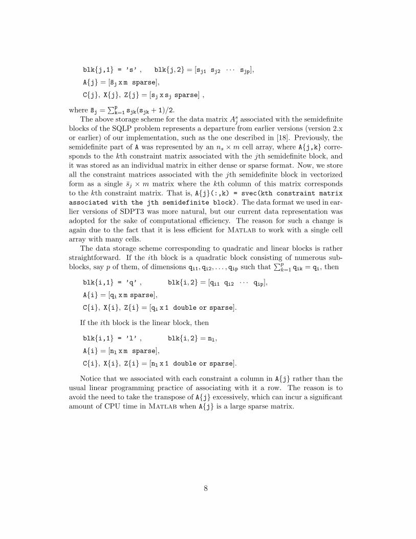
blk{j,1} = ’s’ , blk{j, 2} = [sj1 sj2 · · · sjp],

A{j} = [sj x m sparse],

C{j}, X{j}, Z{j} = [sj x sj sparse] ,

where sj =∑p

k=1 sjk(sjk + 1)/2.The above storage scheme for the data matrix Asj associated with the semidefinite

blocks of the SQLP problem represents a departure from earlier versions (version 2.xor earlier) of our implementation, such as the one described in [18]. Previously, thesemidefinite part of A was represented by an ns ×m cell array, where A{j,k} corre-sponds to the kth constraint matrix associated with the jth semidefinite block, andit was stored as an individual matrix in either dense or sparse format. Now, we storeall the constraint matrices associated with the jth semidefinite block in vectorizedform as a single sj × m matrix where the kth column of this matrix correspondsto the kth constraint matrix. That is, A{j}(:,k) = svec(kth constraint matrixassociated with the jth semidefinite block). The data format we used in ear-lier versions of SDPT3 was more natural, but our current data representation wasadopted for the sake of computational efficiency. The reason for such a change isagain due to the fact that it is less efficient for Matlab to work with a single cellarray with many cells.

The data storage scheme corresponding to quadratic and linear blocks is ratherstraightforward. If the ith block is a quadratic block consisting of numerous sub-blocks, say p of them, of dimensions qi1, qi2, . . . , qip such that

∑pk=1 qik = qi, then

blk{i,1} = ’q’ , blk{i, 2} = [qi1 qi2 · · · qip],

A{i} = [qi x m sparse],

C{i}, X{i}, Z{i} = [qi x 1 double or sparse].

If the ith block is the linear block, then

blk{i,1} = ’l’ , blk{i, 2} = nl,

A{i} = [nl x m sparse],

C{i}, X{i}, Z{i} = [nl x 1 double or sparse].

Notice that we associated with each constraint a column in A{j} rather than theusual linear programming practice of associating with it a row. The reason is toavoid the need to take the transpose of A{j} excessively, which can incur a significantamount of CPU time in Matlab when A{j} is a large sparse matrix.

8

3 The search direction

To simplify discussion, we introduce the following notation, which is also consistentwith the internal data representation in SDPT3:

As =

As1...

Asns

, Aq =

Aq1...

Aqnq

.Similarly, we define

xs =

svec(xs1)...

svec(xsns)

, xq =

xq1...xqnq

. (2)

The vectors cs, zs, cq, and zq are defined analogously. We will use correspondingnotation for the search directions as well. Finally, let

A =

As

Aq

Al

, x =

xs

xq

xl

, c =

cs

cq

cl

, z =

zs

zq

zl

,and

n =ns∑j=1

sj +nq∑i=1

qi + nl.

Note that the matrix A above is defined as the transpose of that in the standardliterature so as to be consistent with our data representation.

With the notation introduced above, the primal and dual equality constraints canbe represented respectively as

ATx = b, Ay + z = c.

The primal-dual path-following algorithm we implemented assumes that A has fullcolumn rank. But in our software, the presence of (nearly) dependent constraintsis detected automatically, and warning messages are displayed if such constraintsexist. When this happens, the user has the option of removing these (nearly) de-pendent constraints by calling a preprocessing routine to remove them by settingOPTIONS.rmdepconstr = 1. We should mention that the routine we have coded forremoving dependent constraints is a rather primitive one, and it is inefficient for largeproblems. We hope to improve on this routine in future versions of SDPT3.

The main step at each iteration of our algorithms is the computation of the searchdirection (∆x,∆y,∆z) from the symmetrized Newton equation with respect to aninvertible block diagonal scaling matrix P for the semidefinite block and an invertibleblock diagonal scaling matrix G for the quadratic block. The matrices P and G are

9

usually chosen as functions of the current iterate x, z and we will elaborate on specificchoices below. The search direction (∆x,∆y,∆z) is obtained from the followingsystem of equations:

A∆y + ∆z = Rd := c− z −AyAT∆x = rp := b−ATxEs∆xs + Fs∆zs = Rsc := svec (σµI −HP (smat(xs)smat(zs)))

Eq∆xq + Fq∆zq = Rqc := σµeq − TG(xq, zq)

E l∆xl + F l∆zl = Rlc := σµel − E lF lel,

(3)

where µ = 〈x, z〉/n and σ is the centering parameter. The notation smat denotesthe inverse map of svec and both are to be interpreted as blockwise operators if theargument consists of blocks. Here HP is the symmetrization operator whose actionon the jth semidefinite block is defined by

HPj : IRsj×sj −→ IRsj×sj

HPj (U) = 12

[PjUP

−1j + P−Tj UTP Tj

], (4)

with Pj the jth block of the block diagonal matrix P and Es and Fs are symmetricblock diagonal matrices whose jth blocks are given by

Esj = Pj©∗ P−Tj zsj , Fsj = Pjxsj ©∗ P−Tj , (5)

where R©∗ T is the symmetrized Kronecker product operation described in [15].In the quadratic block, eq denotes the blockwise identity vector, i.e.,

eq =

eq1...eqnq

,where eqi is the first unit vector in IRqi . Let the arrow operator defined in [2] bedenoted by Arw (·). Then the operator TG is defined as follows:

TG(xq, zq) =

Arw (G1x

q1) (G−1

1 zq1)...

Arw(Gnqx

qnq

)(G−1

nq zqnq)

, (6)

where G is a symmetric block diagonal matrix that depends on x, z and Gi is the ithblock of G. The matrices Eq and Fq are block diagonal matrices whose the ith blocksare given by

Eqi = Arw(G−1i zqi

)Gi, Fqi = Arw (Gix

qi )G

−1i . (7)

10

In the linear block, el denotes the nl-dimensional vector of ones, and E l = diag(xl),F l = diag(zl).

For future reference, we partition the vectors Rd, ∆x, and ∆z in a manner anal-ogous to c, x, and z as follows:

Rd =

Rsd

Rqd

Rld

, ∆x =

∆xs

∆xq

∆xl

, ∆z =

∆zs

∆zq

∆zl

. (8)

Assuming that m = O(n), we compute the search direction via a Schur comple-ment equation as follows (the reader is referred to [1] and [15] for details). Firstcompute ∆y from the Schur complement equation

M∆y = h, (9)

where

M = (As)T (Es)−1FsAs + (Aq)T (Eq)−1FqAq + (Al)T (E l)−1F lAl (10)

h = rp − (As)T (Es)−1(Rsc −FsRsd)− (Aq)T (Eq)−1(Rqc −FqR

qd) − (Al)T (E l)−1(Rlc −F lRld). (11)

Then compute ∆x and ∆z from the equations

∆z = Rd −A∆y (12)

∆xs = (Es)−1Rsc − (Es)−1Fs∆zs (13)

∆xq = (Eq)−1Rqc − (Eq)−1Fq∆zq (14)

∆xl = (E l)−1Rlc − (E l)−1F l∆zl. (15)

3.1 Two choices of search directions

We start by introducing some notation that we will use in the remainder of thispaper. For a given qi-dimensional vector xqi , we let x0

i denote its first component andx1i denote its subvector consisting of the remaining entries, i.e.,[

x0i

x1i

]=

[(xqi )1

(xqi )2:qi

]. (16)

We will use the same convention for zqi , ∆xqi , etc. Also, we define the followingfunction from Kqi

q to IR+:

γ(xqi ) :=√

(x0i )2 − 〈x1

i , x1i 〉. (17)

Finally, we use X and Z for smat(xs) and smat(zs), where the operation is appliedblockwise to form a block diagonal symmetric matrix of order

∑nsj=1 sj .

11

In the current release of this package, the user has two choices of scaling operatorsparametrized by P and G, resulting in two different search directions: the HKMdirection [7, 9, 11], and the NT direction [14]. See also Tsuchiya [20] for the second-order case.

(1) The HKM direction. This choice uses the scaling matrix P = Z1/2 for thesemidefinite blocks and a symmetric block diagonal scaling matrix G for thequadratic blocks where the ith block Gi is given by the following equation:

Gi =

z0i (z1

i )T

z1i γ(zqi )I +

z1i (z1

i )T

γ(zqi ) + z0i

. (18)

(2) The NT direction. This choice uses the scaling matrix P = N−1 for thesemidefinite blocks, where N is a matrix such that D := NTZN = N−1XN−T

is a diagonal matrix [15], and G is a symmetric block diagonal matrix whose ithblock Gi is defined as follows. Let

ωi =

√γ(zqi )γ(xqi )

, ξi =

[ξ0i

ξ1i

]=

[ 1ωiz0i + ωix

0i

1ωiz1i − ωix1

i

]. (19)

Then

Gi = ωi

t0i (t1i )T

t1i I +t1i (t

1i )T

1 + t0i

, where

[t0i

t1i

]=

1γ(ξi)

[ξ0i

ξ1i

]. (20)

3.2 Computation of the search directions

Generally, the most expensive part in each iteration of Algorithm IPC lies in thecomputation and factorization of the Schur complement matrix M defined in (9).And this depends critically on the size and density of M . Note that the densityof this matrix depends on two factors: (i) The density of the constraint coefficientmatrices As, Aq, and Al, and (ii) any additional fill-in introduced because of theterms (Es)−1Fs, (Eq)−1Fq, and (E l)−1F l in (9).

3.2.1 Semidefinite blocks

For problems with semidefinite blocks, the contribution by the jth semidefinite blockto M is given by M s

j := (Asj)T (Esj )−1FsjAsj . As the matrix (Esj )−1Fsj is dense and

structure-less for most problems, the matrix M sj is generally dense even if Asj is

sparse. The computation of each entry of M sj involves matrix products, which in the

case of NT direction has the form

(M sj )αβ = Asj(:, α)T svec

(wsj smat(Asj(:, β))wsj

),

12

where Asj(:, k) denotes the kth column of Asj . This computation can be very expensiveif it is done naively without properly the exploiting sparsity that is generally presentin Asj . In our earlier papers [15, 18], we discussed briefly how sparsity of Asj isexploited in our implementation by following the ideas presented in [4]. However, asthe efficient implementation of these ideas is not spelled out in the current literature,we will provide further details here.

In our implementation, firstly the matrix Asj is sorted column-wise in ascendingorder of the number of non-zero elements in each column. Suppose we denote thesorted matrix by Asj and the matrix (Asj)

T (Esj )−1Fsj Asj by M sj . (We should emphasize

that, in order to cut down memory usage, the matrix Asj is not created explicitly, butit is accessed through Asj via a permutation vector, and similarly for M s

j .) Then a2-column cell array nzlistA is created such that nzlistA{j,1} is an m-vector wherenzlistA{j,1}(k) is the starting row index in the 2-column matrix nzlistA{j,2}that stores the row and column indices of the non-zero elements of smat(Asj(:, k)).If the number of non-zero elements of smat(Asj(:, k)) exceeds a certain threshold, weset nzlistA{j,1}(k) = inf, and we do not append the row and column indices ofthis matrix to nzlistA{j,2}. We use the flag “inf” to indicate that the density ofthe matrix is too high for sparse computation to be done efficiently. If J is the largestinteger for which nzlistA{j,1}(k) < inf, then we compute the upper triangularpart of matrix M s

j (1 : J, 1 : J) through formula F-3 described in [4]. In our software,this part of the computation is done in a C Mex routine mexschur.mex*.

As formula F-3 is efficient only for very sparse constraint matrices, say with den-sity below the level of 2%, we also need to handle the case where constraint matriceshave a moderate level of density, say 2% − 20%. For such matrices, the strategy isto compute only those elements of the matrix product U := wsj smat(Asj(:, β))wsjthat contribute to an entry of M s

j , that is, those that correspond to a nonzeroentry of Asj(:, k) for some k = 1, . . . , β. Basically, we use formula F-2 describedin [4] in this case. In our implementation, we create another 2-column cell arraynzlistAsum to facilitate such calculations. In this case, nzlistAsum{j,1} is a vec-tor such that nzlistAsum{j,1}(k) is the starting row index in the 2-column matrixnzlistAum{j,2} that stores the row and column indices of the non-zero elementsof smat(Asj(:, k)) that are not already present in the combined list of non-zero ele-ments from

∑k−1i=1 |smat(Asj(:, i))|. Again, if the combined list of non-zero elements

of∑ki=1 |smat(Asj(:, i))| exceeds a certain threshold, we set nzlistAsum{j,1}(k) =

inf since formula F-2 in [4] is not efficient when the combined list of non-zeros ele-ments that need to be calculated for U is too large. Suppose L is the largest integersuch that nzlistAsum{j,1}(k) < inf. Then we compute the upper triangular partof M s

j (1 : L, J : L) through formula F-2. Again, for efficiency, we do the computationin a C Mex routine mexProd2nz.mex*.

The remaining columns of M sj are calculated by first computing the full matrix

U , and then taking the inner product between the appropriate columns of Asj andsvec(U).

Finally, we would like to highlight an issue that is often critical in cutting down

13

the computation time in forming M sj . In many large SDP problems, the matrix

smat(Asj(:, k)) is usually sparse, and it is important to store this matrix as a sparsematrix in Matlab and perform sparse-dense matrix-matrix multiplication wheneverpossible.

3.2.2 Quadratic and linear blocks

For linear blocks, (E l)−1F l is a diagonal matrix and it does not introduce any addi-tional fill-in. This matrix does, however, affect the conditioning of the Schur comple-ment matrix and is a popular subject of research in implementations of interior-pointmethods for linear programming.

From equation (10), it is easily shown that the contribution of the quadratic blocksto the matrix M is given by

M q = (Aq)T (Eq)−1FqAq =nq∑i=1

(Aqi )T (Eqi )−1Fqi A

qi︸ ︷︷ ︸

Mqi

. (21)

For the HKM direction, (Eqi )−1Fqi is a diagonal matrix plus a rank-two symmetricmatrix, and we have

M qi =

〈xqi , zqi 〉

γ2(zqi )(Aqi )

TJiAqi + uqi (v

qi )T + vqi (u

qi )T , (22)

where

Ji =

[−1 00 I

], uqi = (Aqi )

T

[x0i

x1i

], vqi = (Aqi )

T

(1

γ2(zqi )

[z0i

−z1i

]). (23)

The appearance of the outer-product terms in the equation above is potentiallyalarming. If the vectors uqi , v

qi are dense, then even if Aqi is sparse, the corresponding

matrix M qi , and hence the Schur complement matrix M , will be dense. A direct

factorization of the resulting dense matrix will be very expensive for even moderatelyhigh m.

The observed behavior of the density of the matrix M qi on test problems depends

largely on the particular problem structure. When the problem has many smallquadratic blocks, it is often the case that each block appears in only a small fractionof the constraints. In this case, all Aqi matrices are sparse and the vectors uqi andvqi turn out to be sparse vectors for each i. Consequently, the matrices M q

i remainrelatively sparse for these problems. As a result, M is also sparse and it can befactorized directly with reasonable cost. The behavior is typical for all nql and qsspproblems from the DIMACS library.

The situation is drastically different for problems where one of the quadraticblocks, say the ith block, is large. For such problems the vectors uqi , v

qi are typically

dense, and therefore, M qi is likely be a dense matrix even if the data Aqi is sparse.

However, observe that M qi is a rank-two perturbation of a sparse matrix when Aqi is

14

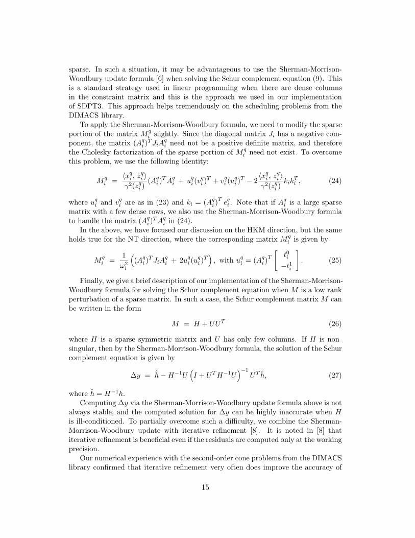
sparse. In such a situation, it may be advantageous to use the Sherman-Morrison-Woodbury update formula [6] when solving the Schur complement equation (9). Thisis a standard strategy used in linear programming when there are dense columnsin the constraint matrix and this is the approach we used in our implementationof SDPT3. This approach helps tremendously on the scheduling problems from theDIMACS library.

To apply the Sherman-Morrison-Woodbury formula, we need to modify the sparseportion of the matrix M q

i slightly. Since the diagonal matrix Ji has a negative com-ponent, the matrix (Aqi )

TJiAqi need not be a positive definite matrix, and therefore

the Cholesky factorization of the sparse portion of M qi need not exist. To overcome

this problem, we use the following identity:

M qi =

〈xqi , zqi 〉

γ2(zqi )(Aqi )

TAqi + uqi (vqi )T + vqi (u

qi )T − 2

〈xqi , zqi 〉

γ2(zqi )kik

Ti , (24)

where uqi and vqi are as in (23) and ki = (Aqi )Teqi . Note that if Aqi is a large sparse

matrix with a few dense rows, we also use the Sherman-Morrison-Woodbury formulato handle the matrix (Aqi )

TAqi in (24).In the above, we have focused our discussion on the HKM direction, but the same

holds true for the NT direction, where the corresponding matrix M qi is given by

M qi =

1ω2i

((Aqi )

TJiAqi + 2uqi (u

qi )T), with uqi = (Aqi )

T

[t0i−t1i

]. (25)

Finally, we give a brief description of our implementation of the Sherman-Morrison-Woodbury formula for solving the Schur complement equation when M is a low rankperturbation of a sparse matrix. In such a case, the Schur complement matrix M canbe written in the form

M = H + UUT (26)

where H is a sparse symmetric matrix and U has only few columns. If H is non-singular, then by the Sherman-Morrison-Woodbury formula, the solution of the Schurcomplement equation is given by

∆y = h−H−1U(I + UTH−1U

)−1UT h, (27)

where h = H−1h.Computing ∆y via the Sherman-Morrison-Woodbury update formula above is not

always stable, and the computed solution for ∆y can be highly inaccurate when His ill-conditioned. To partially overcome such a difficulty, we combine the Sherman-Morrison-Woodbury update with iterative refinement [8]. It is noted in [8] thatiterative refinement is beneficial even if the residuals are computed only at the workingprecision.

Our numerical experience with the second-order cone problems from the DIMACSlibrary confirmed that iterative refinement very often does improve the accuracy of

15

the computed solution for ∆y via the Sherman-Morrison-Woodbury formula. How-ever, we must mention that iterative refinement can occasionally fail to provide anysignificant improvement. We have not yet incorporated a stable and efficient methodfor computing ∆y when M has the form (26), but note that Goldfarb and Scheinberg[5] discuss a stable product-form Cholesky factorization approach to this problem.

3.3 Step-length computation

Once a direction ∆x is computed, a full step will not be allowed if x + ∆x violatesthe conic constraints. Thus, the next iterate must take the form x + α∆x for anappropriate choice of the step-length α. In this subsection, we discuss an efficientstrategy to compute the step-length α.

For semidefinite blocks, it is straightforward to verify that, for the jth block,the maximum allowed step-length that can be taken without violating the positivesemidefiniteness of the matrix xsj + αsj∆x

sj is given as follows:

αsj =

−1

λmin((xsj)−1∆xsj), if the minimum eigenvalue λmin is negative

∞ otherwise.(28)

If the computation of eigenvalues necessary in αsj above becomes expensive, then weresort to finding an approximation of αsj by estimating extreme eigenvalues usingLanczos iterations [17]. This approach is quite accurate in general and representsa good trade-off between the computational effort versus quality of the resultingstepsizes.

For quadratic blocks, the largest step-length αqi that keeps the next iterate feasiblewith respect to the kth quadratic cone can be computed as follows. Let

ai = γ2(∆xqi ), bi = 〈∆xqi , −Jixqi 〉, ci = γ2(xqi ), di = b2i − aici,

where Ji is the matrix defined in (23). We want the largest positive α for whichaiα

2 + 2biα+ ci > 0 for all smaller positive α’s, which is given by

αqi =

−bi −√di

aiif ai < 0 or bi < 0, ai ≤ b2i /ci

−ci2bi

if ai = 0, bi < 0

∞ otherwise.

For the linear block, the maximum allowed step-length αli for the hth componentis given by

αlh =

−xlh∆xlh

, if ∆xlh < 0

∞ otherwise.

16

Finally, an appropriate step-length α that can be taken in order for x+α∆x to satisfyall the conic constraints takes the form

α = min(

1, γ min1≤j≤ns

αsj , γ min1≤i≤nq

αqi , γ min1≤h≤nl

αlh

), (29)

where γ (known as the step-length parameter) is typically chosen to be a numberslightly less than 1, say 0.98, to ensure that the next iterate x + α∆x stays strictlyin the interior of all the cones.

For the dual direction ∆z, we let the analog of αsj , αqi and αlh be βsj , β

qi and βlh,

respectively. Similar to the primal direction, the step-length that can be taken bythe dual direction ∆z is given by

β = min(

1, γ min1≤j≤ns

βsj , γ min1≤i≤nq

βqi , γ min1≤h≤nl

βlh

). (30)

4 Further details

Sample runs.

We will now generate some sample runs to illustrate how our package might be usedto solve test problems from the SDPLIB and DIMACS libraries [3, 13]. We providetwo m-files, read sdpa.m and read sedumi.m, to convert problem data from theselibraries into Matlab cell arrays described in Section 2. We assume that the currentdirectory is SDPT3-3.0 and sdplib is a subdirectory.

>> startup % set up default parameters in the OPTIONS structure>> [blk,A,C,b] = read_sdpa(’./sdplib/mcp250.1.dat-s’);>> [obj,X,y,Z] = sqlp(blk,A,C,b);

*******************************************************************Infeasible path-following algorithms

*******************************************************************version predcorr gam expon scale_dataHKM 1 0.000 1 0

it pstep dstep p_infeas d_infeas gap obj cputime-------------------------------------------------------------------0 0.000 0.000 1.8e+02 1.9e+01 7.0e+05 -1.462827e+041 0.981 1.000 3.3e+00 2.0e-15 1.7e+04 -2.429708e+03 0.72 1.000 1.000 4.3e-14 0.0e+00 2.4e+03 -1.352811e+03 2.2: : : : : : : :13 1.000 0.996 3.9e-13 8.6e-17 2.1e-05 -3.172643e+02 19.214 1.000 1.000 4.1e-13 8.9e-17 6.5e-07 -3.172643e+02 20.6

Stop: max(relative gap, infeasibilities) < 1.00e-08----------------------------------------------------number of iterations = 14gap = 6.45e-07relative gap = 2.03e-09

17

primal infeasibilities = 4.13e-13dual infeasibilities = 8.92e-17Total CPU time (secs) = 21.8CPU time per iteration = 1.6termination code = 0-------------------------------------------------------------------Percentage of CPU time spent in various parts-------------------------------------------------------------------preproc Xchol Zchol pred pred_steplen corr corr_steplen misc5.7 3.6 0.5 33.3 9.5 3.9 25.2 11.1 3.9 3.3

-------------------------------------------------------------------

We can solve a DIMACS test problem in a similar manner.

>> OPTIONS.vers = 2; % use NT direction>> [blk,A,C,b] = read_sedumi(’./dimacs/nb.mat’);>> [obj,X,y,Z] = sqlp(blk,A,C,b,[],[],[],OPTIONS);

******************************************************************Infeasible path-following algorithms

*******************************************************************version predcorr gam expon scale_data

NT 1 0.000 1 0it pstep dstep p_infeas d_infeas gap obj cputime-------------------------------------------------------------------0 0.000 0.000 1.4e+03 5.8e+02 4.0e+04 0.000000e+001 0.981 0.976 2.6e+01 1.4e+01 7.8e+02 -1.423573e+01 2.82 1.000 0.989 1.2e-14 1.5e-01 2.7e+01 -1.351345e+01 6.4: : : : : : : :13 0.676 0.778 2.6e-05 1.4e-08 2.4e-04 -5.059624e-02 45.714 0.210 0.463 2.6e-04 7.7e-09 1.9e-04 -5.061370e-02 49.3

Stop: relative gap < 5*infeasibility----------------------------------------------------number of iterations = 14gap = 1.89e-04relative gap = 1.89e-04primal infeasibilities = 2.57e-04dual infeasibilities = 7.65e-09Total CPU time (secs) = 51.3CPU time per iteration = 3.7termination code = 0-------------------------------------------------------------------Percentage of CPU time spent in various parts-------------------------------------------------------------------preproc Xchol Zchol pred pred_steplen corr corr_steplen misc4.0 0.2 0.1 90.0 0.2 0.1 2.6 0.1 0.3 2.3

-------------------------------------------------------------------

Note that in this example, dual feasibility is almost attained, while primal feasibilitywas attained at iteration 2 but has since been slowly degrading. The iterations

18

terminate when this degradation overtakes the improvement in the duality gap (thisis part of Item 4 in our list of stopping criteria in Section 2).

Mex files used.

Our software uses a number of Mex routines generated from C programs written tocarry out certain operations that Matlab is not efficient at. In particular, operationssuch as extracting selected elements of a matrix, and performing arithmetic opera-tions on these selected elements are all done in C. As an example, the vectorizationoperation svec is coded in the C program mexsvec.c.

Our software also uses a number of Mex routines generated from Fortran programswritten by Ng, Peyton, and Liu for computing sparse Cholesky factorizations [12].These programs are adapted from the LIPSOL software written by Y. Zhang [21].

To generate these Mex routines, the user can run the shell script file Installmexin the subdirectory SDPT3-3.0/Solver/mexsrc by typing ./Installmex in that sub-directory.

Cholesky factorization.

Earlier versions of SDPT3 were intended for problems that always have semidefinitecone constraints. For SDP problems, the Schur complement matrix M in (10) isgenerally a dense matrix after the first iteration. To solve the associated linear system(9), we first find a Cholesky factorization of M and then solve two triangular systems.When M is dense, a reordering of the rows and columns of M does not alter theefficiency of the Cholesky factorization and specialized sparse Cholesky factorizationroutines are not useful. Therefore, earlier versions of SDPT3 (up to version 1.3)simply used Matlab’s chol routine for Cholesky factorizations. For versions 2.1 and2.2, we introduced our own Cholesky factorization routine mexchol that utilizes loopunrolling and provided 2-fold speed-ups on some architectures compared to Matlab’schol routine. However, in newer versions of Matlab that use numerics libraries basedon LAPACK, Matlab’s chol routine is more efficient than our Cholesky factorizationroutine mexchol for dense matrices. Thus, in version 3.0, we use Matlab’s cholroutine whenever M is dense.

For most second-order cone programming problems in the DIMACS library, how-ever, Matlab’s chol routine is not competitive. This is largely due to the fact thatthe Schur complement matrix M is often sparse for SOCPs and LPs, and Matlab

cannot sufficiently take advantage of this sparsity. To solve such problems moreefficiently we imported the sparse Cholesky solver in Y. Zhang’s LIPSOL [21], aninterior-point code for linear programming problems. It should be noted that LIP-SOL uses Fortran programs developed by Ng, Peyton, and Liu for Cholesky factoriza-tion [12]. When SDPT3 uses LIPSOL’s Cholesky solver, it first generates a symbolicfactorization of the Schur complement matrix to determine the pivot order by exam-ining the sparsity structure of this matrix carefully. Then, this pivot order is re-usedin later iterations to compute the Cholesky factors. Contrary to the case of linearprogramming, however, the sparsity structure of the Schur complement matrix can

19

change during the iterations for SOCP problems. If this happens, the pivot orderhas to be recomputed. We detect changes in the sparsity structure by monitoring thenonzero elements of the Schur complement matrix. Since the default initial iterateswe use for an SOCP problem are unit vectors but subsequent iterates are not, thereis always a change in the sparsity pattern of M after the first iteration. After thesecond iteration, the sparsity pattern remains unchanged for most problems, and onlyone more change occurs in a small fraction of the test problems.

The effect of including a sparse Cholesky solver option for SOCP problems wasdramatic. We observed speed-ups of up to two orders of magnitude. Version 3.0 ofSDPT3 automatically makes a choice between Matlab’s built-in chol routine andthe sparse Cholesky solver based on the density of the Schur complement matrix.The cutoff density is specified in the parameter OPTIONS.spdensity.

Vectorized matrices vs. sparse matrices.

The current release, version 3.0, of the code stores the constraint matrix in “vector-ized” form as described in Section 2. In the previous version 2.3, A was a doublysubscripted cell array of symmetric matrices for the semidefinite blocks. The resultof the change is that much less storage is required for the constraint matrix, and thatwe save a considerable amount of time in forming the Schur complement matrix Min (10) by avoiding loops over the index k. An analysis of the amount of time version3.0 of our code spends on different parts of the algorithm leads to the following obser-vations, which can sometimes be platform dependent: Operations relating to formingand factorizing the Schur complement and hence computing the predictor search di-rection comprise much of the computational work for most problem classes, rangingfrom about 25% for qpG11 up to 99% for the larger theta problems, the controlproblems, copo14, hamming-7-5-6, and the nb problems. Other parts of the codethat require significant amount of computational time include the computation of thecorrector search direction (up to 51% on some qp problems) and the computation ofstep lengths (up to 50% on truss7).

While we now store the constraint matrix in vectorized form, the parts of theiterates X and Z corresponding to semidefinite blocks are still stored as matrices,since that is how the user wants to access them.

Choice of search direction.

The new version of the code allows only two search directions, HKM and NT. Version2.3 also allowed the AHO direction of Alizadeh, Haeberly, and Overton [1] and theGT (Gu-Toh, see [16]) direction, but these options are not competitive when theproblems are of large scale. We intend to keep version 2.3 of the code available forthose who wish to experiment with these other search directions, which tend to givemore accurate results on smaller problems.

For the two remaining search directions, our computational experience on prob-lems from the SDPLIB and DIMACS libaries is that the HKM direction is almostuniversally faster than NT on problems with semidefinite blocks, especially for sparse

20

problems with large semidefinite blocks such as the equalG and maxG problems. Thereason that the latter is slower is due to the NT direction’s need to compute an eigen-value decomposition to calculate the NT scaling matrix wsj . This computation candominate the work in each interior-point iteration when the problem is sparse.

The NT direction, however, was faster on SOCP problems such as the nb, nql,and sched problems. The reason for this behavior is not hard to understand. Bycomparing the formula in (22) for the HKM direction with (25) for the NT direction, itis clear that more computation is required to assemble the Schur complement matrixand more low-rank updating is necessary for the former direction.

Real vs. complex data.

In earlier versions, we allowed SDP problems with complex data, i.e., the constraintmatrices are hermitian matrices. However, as problems with complex data rarelyoccur in practice, and in an effort to simplify the code, we removed this flexibility inthe current version. But we intend to keep version 2.3 of the code available for userswho wish to solve SDP problems with complex data.

Homogeneous vs. infeasible interior-point methods.

Version 2.3 also allowed the user to employ homogeneous self-dual algorithms insteadof the usual infeasible interior-point methods. However, this option almost alwaystook longer than the default choice, and so it has been omitted from the currentrelease. One theoretical advantage of the homogeneous self-dual approach is that itis oriented towards either producing optimal primal and dual solutions or generatinga certificate of primal or dual infeasibility, while the infeasible methods strive foroptimal solutions only, but detect infeasibility if either the dual or primal iteratesdiverge. However, we have observed no advantage to the homogeneous methodswhen applied to infeasible problems. We should mention, however, that our currentversion does not detect infeasibility in the problem filtinf1, but instead stops with aprimal near-feasible solution and a dual feasible solution when it encounters numericalproblems.

Specifying the block structure of problems.

Our software requires the user to specify the block structure of the SQLP prob-lem. Although no technical difficulty will arise if the user choose to lump a fewblocks together and consider it as a single large block, the computational timecan be dramatically different. For example, the problem qpG11 in the SDPLIB li-brary actually has block structure blk{1,1} = ’s’, blk{1,2} = 800, blk{2,1} =’l’, blk{2,2}=800, but the structure specified in the library is blk{1,1} = ’s’,blk{1,2} = 1600. That is, in the former, the linear variables are explicitly identi-fied, rather than being part of a large sparse semidefinite block. The difference inthe running time for specifying the block structure differently is dramatic: the formerrepresentation is at least six times faster when the HKM direction is used, besides

21

using much less memory space.It is thus crucial to present problems to the algorithms correctly. We could add

our own preprocessor to detect this structure, but believe users are aware of linearvariables present in their problems. Unfortunately the versions of qpG11 (and alsoqpG51) in SDPLIB do not show this structure explicitly. In our software, we providedan m-file, detect diag.m, to detect and correct problems with hidden linear variables.The user can call this m-file after loading the problem data into Matlab as follows:

>> [blk,A,C,b] = read_sdpa(’../SDPtest/sdplib/qpG11.dat-s’);>> [blk,A,C,b] = detect_diag(blk,A,C,b);

Finally, version 2.3 of SDPT3 included specialized routines to compute the Schurcomplement matrices directly for certain classes of problem (e.g., maxcut problems).In earlier versions of SDPT3, these specialized routines had produced dramatic de-creases in solution times, but for version 2.3, these gains were marginal, since our CMex routines for exploiting sparsity in computing the Schur complement matrix pro-vided almost as much speedup. We have therefore dropped these routines in version3.0.

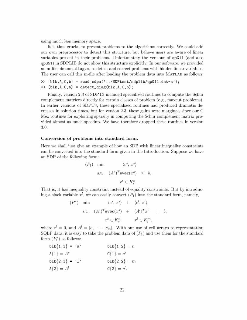
Conversion of problems into standard form.

Here we shall just give an example of how an SDP with linear inequality constraintscan be converted into the standard form given in the Introduction. Suppose we havean SDP of the following form:

(P1) min 〈cs, xs〉

s.t. (As)T svec(xs) ≤ b,

xs ∈ Kns .

That is, it has inequality constraint instead of equality constraints. But by introduc-ing a slack variable xl, we can easily convert (P1) into the standard form, namely,

(P ∗1 ) min 〈cs, xs〉 + 〈cl, xl〉

s.t. (As)T svec(xs) + (Al)Txl = b,

xs ∈ Kns . xl ∈ Km

l ,

where cl = 0, and Al = [e1 · · · em]. With our use of cell arrays to representationSQLP data, it is easy to take the problem data of (P1) and use them for the standardform (P ∗1 ) as follows:

blk{1,1} = ’s’ blk{1,2} = n

A{1} = As C{1} = cs

blk{2,1} = ’l’ blk{2,2} = m

A{2} = Al C{2} = cl.

22

Caveats.

The user should be aware that SQLP is more complicated than linear programming.For example, it is possible that both primal and dual problems are feasible, buttheir optimal values are not equal. Also, either problem may be infeasible withoutthere being a certificate of that fact (so-called weak infeasibility). In such cases, oursoftware package is likely to terminate after some iterations with an indication ofshort step-length or lack of progress. Also, even if there is a certificate of infeasibility,our infeasible-interior-point methods may not find it. In our very limited testing onstrongly infeasible problems, most of our algorithms have been quite successful indetecting infeasibility.

5 Computational results

Here we describe the results of our computational testing of SDPT3, on problems fromthe SDPLIB collection of Borchers [3] as well as the DIMACS library test problems[13]. In both, we solve a selection of the problems; in the DIMACS problems, theseare selected as the more tractable problems, while our subset of the SDPLIB problemsis more representative (but we cannot solve the largest two maxG problems). Sinceour algorithm is a primal-dual method storing the primal iterate X, it cannot exploitcommon sparsity in C and the constraint matrices as effectively as dual methods ornonlinear-programming based methods. We are therefore unable to solve the largestproblems.

The test problems are listed in Tables 1 and 2, along with their dimensions. Theresults given were obtained on a Pentium III PC (800MHz) with 1G of memoryrunning Linux, using Matlab 6.0. (We had some difficulties with Matlab 6 usingsome of our codes on a Solaris platform, possibly due to bugs in the Solaris versionof Matlab 6.)

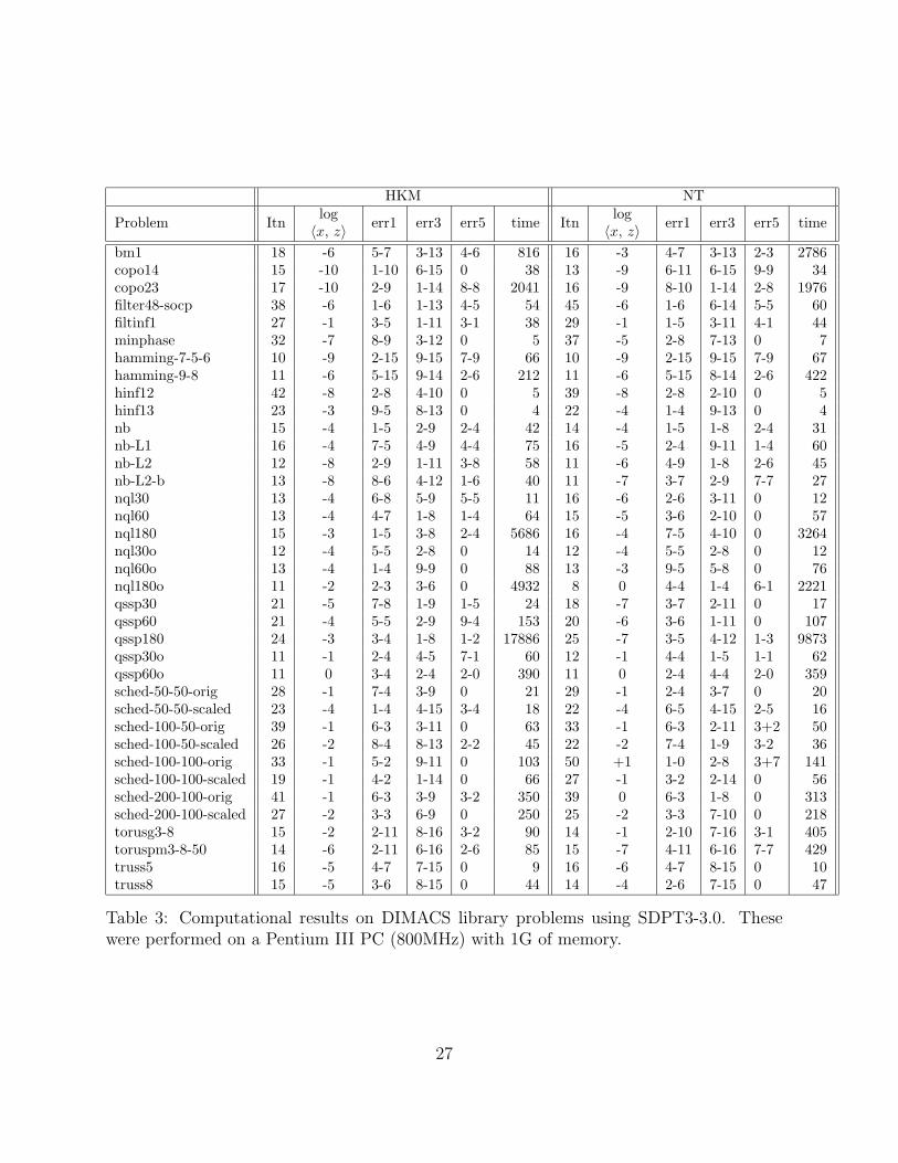
Results are given in Tables 3 and 4: Table 3 summarizes the results of our compu-tational experiments on the DIMACS set of problems, while the corresponding resultsfor problems from the SDPLIB library are presented in Table 4. In each table, welist the number of of iterations required, the time in seconds, and four measures ofthe precision of the computed answer for each problem and for both the HKM andthe NT directions. The first of the four accuracy measures is the logarithm (to base10) of the total complementary slackness; the second is the scaled primal infeasibility‖Ax− b‖/(1+max |bk|), and the third is ‖AT y+z− c‖/(1+max |c|), where the normis subordinate to the inner product and the maximum taken over all componentsof c; and the last one is the maximum of 0 and 〈c, x〉 − bT y. Entries like 3 − 13mean 3× 10−13, etc. In accuracy reporting we followed the guidelines set up for theDIMACS Challenge that took place in November 2000. These set of measures aresomewhat inconsistent: the first and the last are absolute measures that do not takethe solution size into account while the other two measures are relative to the sizesof certain input parameters.

Our codes solved most of the problems in the two libraries to reasonable accuracy

23

Problem m semidefinite blocks second-order blocks linear blockbm1 883 882 – –copo14 1275 [14 x 14] – 364copo23 5820 [23 x 23] – 1771copo68 154905 [68 x 68] – 50116filter48-socp 969 48 49 931filtinf1 983 49 49 945minphase 48 48 – –hamming-7-5-6 1793 128 – –hamming-9-8 2305 512 – –hinf12 43 [3, 6, 6, 12] – –hinf13 57 [3, 7, 9, 14] – –nb 123 – [793 x 3] 4nb-L1 915 – [793 x 3] 797nb-L2 123 – [1677, 838 x 3] 4nb-L2-bessel 123 – [123, 838 x 3] 4nql30 3680 – [900 x 3] 3602nql60 14560 – [3600 x 3] 14402nql180 130080 – [32400 x 3] 129602nql30old 3601 – [900 x 3] 5560nql60old 14401 – [3600 x 3] 21920nql180old 129601 – [32400 x 3] 195360qssp30 3691 – [1891 x 4] 2qssp60 14581 – [7381 x 4] 2qssp180 130141 – [65341 x 4] 2qssp30old 5674 – [1891 x 4] 3600qssp60old 22144 – [7381 x 4] 14400qssp180old 196024 – [65341 x 4] 129600sched-50-50-orig 2527 – [2474, 3] 2502sched-50-50-scaled 2526 – 2475 2502sched-100-50-orig 4844 – [4741, 3] 5002sched-100-50-scaled 4843 – 4742 5002sched-100-100-orig 8338 – [8235, 3] 10002sched-100-100-scaled 8337 – 8236 10002sched-200-100-orig 18087 – [17884, 3] 20002sched-200-100-scaled 18086 – 17885 20002torusg3-8 512 512 – –toruspm3-8-50 512 512 – –truss5 208 [33 x 10, 1] – –truss8 496 [33 x 19, 1] – –

Table 1: Selected DIMACS library problems. Notation like [33 x 19] indicates that therewere 33 semidefinite blocks, each a symmetric matrix of order 19, etc.

24

Problem m semidefinite blocks linear blockarch8 174 161 174control7 666 [70, 35] –control10 1326 [100, 50] –control11 1596 [110, 55] –gpp250-4 251 250 –gpp500-4 501 500 –hinf15 91 37 –mcp250-1 250 250 –mcp500-1 500 500 –qap9 748 82 –qap10 1021 101 –ss30 132 294 132theta3 1106 150 –theta4 1949 200 –theta5 3028 250 –theta6 4375 300 –truss7 86 [150 x 2, 1] –truss8 496 [33 x 19, 1] –equalG11 801 801 –equalG51 1001 1001 –equalG32 2001 2001 –maxG11 800 800 –maxG51 1000 1000 –maxG32 2000 2000 –qpG11 800 1600 –qpG112 800 800 800qpG51 1000 2000 –qpG512 1000 1000 1000thetaG11 2401 801 –thetaG11n 1601 800 –thetaG51 6910 1001 –thetaG51n 5910 1000 –

Table 2: Selected SDPLIB Problems. Note that qpG112 is identical to qpG11 except thatthe structure of the semidefinite block is exposed as a sparse symmetric matrix of order800 and a diagonal block of the same order, which can be viewed as a linear block, andsimilarly for qpG512. Also, thetaG11n is a more compact formulation of thetaG11, andsimilarly for thetaG51n.

25

— we discuss some of the exceptions. On the DIMACS set of problems, our algo-rithms terminated with low accuracy solutions (measured by 〈x, z〉) on the schedulingproblems and old versions of the nql and qssp problems as well as torusg3-8 andfiltinf1. The last of these problems, filtinf1, is an infeasible problem, but werun into numerical problems before detecting its infeasibility. The optimal values forthe sched*.orig problems and for torusg3-8 are above 105, so the relative accuracy,which may be considered a better measure of accuracy, is acceptable. Both the oldand new versions of the nql and qssp problems contain duplicated columns comingfrom splitting free variables. Feasible sets of the duals of these problems have emptyinteriors and this fact affects the performance of our codes — apparently more so onthe older formulations of these problems. Other measures of accuracy were also rea-sonable for most DIMACS problems, except for, once again, the scheduling problemsand some of the nql and qssp problems.

For the SDPLIB set of problems, we consistently achieve high accuracy solutions,for both the HKM and the NT directions. A few of the smaller problems (hinf15,truss7, and truss8) turn out to be more difficult to solve accurately using eithersearch direction. Interested readers can find detailed discussion of these computa-tional experiments as well as qualitative and quantitative comparisons of differentversions of the code and different search directions in a related article by the authors[19].

References

[1] F. Alizadeh, J.-P. A. Haeberly, and M. L. Overton, Primal-dual interior-pointmethods for semidefinite programming: convergence results, stability and numer-ical results, SIAM J. Optimization, 8 (1998), pp. 746–768.

[2] F. Alizadeh, J.-P. A. Haeberly, M. V. Nayakkankuppam, M. L. Overton, andS. Schmieta, SDPPACK user’s guide, Technical Report, Computer Science De-partment, NYU, New York, June 1997.

[3] B. Borchers, SDPLIB 1.2, a library of semidefinite programming test problems,Optimization Methods and Software, 11 & 12 (1999), pp. 683–690. Available athttp://www.nmt.edu/~borchers/sdplib.html.

[4] K. Fujisawa, M. Kojima, and K. Nakata, Exploiting sparsity in primal-dualinterior-point method for semidefinite programming, Mathematical Program-ming, 79 (1997), pp. 235–253.

[5] D. Goldfarb and K. Scheinberg, A product-form Cholesky factorization im-plementation of an interior-point method for second order cone programming,preprint.

[6] G. H. Golub and C. F. Van Loan, Matrix Computations, 2nd ed., Johns HopkinsUniversity Press, Baltimore, MD, 1989.

26

HKM NT

Problem Itnlog〈x, z〉 err1 err3 err5 time Itn

log〈x, z〉 err1 err3 err5 time

bm1 18 -6 5-7 3-13 4-6 816 16 -3 4-7 3-13 2-3 2786copo14 15 -10 1-10 6-15 0 38 13 -9 6-11 6-15 9-9 34copo23 17 -10 2-9 1-14 8-8 2041 16 -9 8-10 1-14 2-8 1976filter48-socp 38 -6 1-6 1-13 4-5 54 45 -6 1-6 6-14 5-5 60filtinf1 27 -1 3-5 1-11 3-1 38 29 -1 1-5 3-11 4-1 44minphase 32 -7 8-9 3-12 0 5 37 -5 2-8 7-13 0 7hamming-7-5-6 10 -9 2-15 9-15 7-9 66 10 -9 2-15 9-15 7-9 67hamming-9-8 11 -6 5-15 9-14 2-6 212 11 -6 5-15 8-14 2-6 422hinf12 42 -8 2-8 4-10 0 5 39 -8 2-8 2-10 0 5hinf13 23 -3 9-5 8-13 0 4 22 -4 1-4 9-13 0 4nb 15 -4 1-5 2-9 2-4 42 14 -4 1-5 1-8 2-4 31nb-L1 16 -4 7-5 4-9 4-4 75 16 -5 2-4 9-11 1-4 60nb-L2 12 -8 2-9 1-11 3-8 58 11 -6 4-9 1-8 2-6 45nb-L2-b 13 -8 8-6 4-12 1-6 40 11 -7 3-7 2-9 7-7 27nql30 13 -4 6-8 5-9 5-5 11 16 -6 2-6 3-11 0 12nql60 13 -4 4-7 1-8 1-4 64 15 -5 3-6 2-10 0 57nql180 15 -3 1-5 3-8 2-4 5686 16 -4 7-5 4-10 0 3264nql30o 12 -4 5-5 2-8 0 14 12 -4 5-5 2-8 0 12nql60o 13 -4 1-4 9-9 0 88 13 -3 9-5 5-8 0 76nql180o 11 -2 2-3 3-6 0 4932 8 0 4-4 1-4 6-1 2221qssp30 21 -5 7-8 1-9 1-5 24 18 -7 3-7 2-11 0 17qssp60 21 -4 5-5 2-9 9-4 153 20 -6 3-6 1-11 0 107qssp180 24 -3 3-4 1-8 1-2 17886 25 -7 3-5 4-12 1-3 9873qssp30o 11 -1 2-4 4-5 7-1 60 12 -1 4-4 1-5 1-1 62qssp60o 11 0 3-4 2-4 2-0 390 11 0 2-4 4-4 2-0 359sched-50-50-orig 28 -1 7-4 3-9 0 21 29 -1 2-4 3-7 0 20sched-50-50-scaled 23 -4 1-4 4-15 3-4 18 22 -4 6-5 4-15 2-5 16sched-100-50-orig 39 -1 6-3 3-11 0 63 33 -1 6-3 2-11 3+2 50sched-100-50-scaled 26 -2 8-4 8-13 2-2 45 22 -2 7-4 1-9 3-2 36sched-100-100-orig 33 -1 5-2 9-11 0 103 50 +1 1-0 2-8 3+7 141sched-100-100-scaled 19 -1 4-2 1-14 0 66 27 -1 3-2 2-14 0 56sched-200-100-orig 41 -1 6-3 3-9 3-2 350 39 0 6-3 1-8 0 313sched-200-100-scaled 27 -2 3-3 6-9 0 250 25 -2 3-3 7-10 0 218torusg3-8 15 -2 2-11 8-16 3-2 90 14 -1 2-10 7-16 3-1 405toruspm3-8-50 14 -6 2-11 6-16 2-6 85 15 -7 4-11 6-16 7-7 429truss5 16 -5 4-7 7-15 0 9 16 -6 4-7 8-15 0 10truss8 15 -5 3-6 8-15 0 44 14 -4 2-6 7-15 0 47

Table 3: Computational results on DIMACS library problems using SDPT3-3.0. Thesewere performed on a Pentium III PC (800MHz) with 1G of memory.

27

HKM NT

Problem Itnlog〈x, z〉 err1 err3 err5 time Itn

log〈x, z〉 err1 err3 err5 time

arch8 21 -8 1-9 5-13 1-8 42 24 -6 2-8 5-13 2-6 55control7 22 -5 5-7 2-9 3-5 112 22 -5 7-7 2-9 0 131control10 24 -5 1-6 6-9 0 505 24 -5 1-6 6-9 0 610control11 24 -5 2-6 6-9 0 768 23 -4 9-7 6-9 0 890gpp250-4 15 -6 7-8 6-14 0 25 15 -5 6-8 7-14 0 64gpp500-4 15 -5 6-8 4-14 0 156 17 -5 1-8 5-14 1-5 579hinf15 23 -4 9-5 2-12 0 6 22 -4 1-4 2-12 0 7mcp250-1 14 -7 3-12 4-16 6-7 12 15 -7 1-11 4-16 2-7 42mcp500-1 15 -7 1-11 5-16 7-7 62 16 -7 3-11 5-16 3-7 327qap9 15 -5 4-8 5-13 0 17 15 -5 5-8 6-13 0 18qap10 14 -5 4-8 3-13 0 30 13 -4 4-8 5-13 0 30ss30 21 -7 8-9 3-13 5-7 139 24 -6 1-8 2-13 4-6 245theta3 15 -7 2-10 2-14 1-7 38 14 -8 2-10 2-14 3-8 40theta4 15 -7 2-10 3-14 2-7 130 14 -8 3-10 3-14 6-8 135theta5 15 -7 3-10 4-14 2-7 396 14 -8 4-10 4-14 4-8 402theta6 14 -7 2-10 5-14 3-7 975 14 -7 6-10 5-14 1-7 1034truss7 23 -4 3-6 1-13 0 4 21 -4 2-6 2-13 0 5truss8 15 -5 3-6 7-15 0 45 14 -4 2-6 1-14 1-4 47equalG11 17 -6 3-10 3-16 2-6 606 18 -5 7-11 7-15 2-5 2371equalG51 20 -6 2-8 5-16 4-6 1358 20 -6 2-9 1-15 4-6 5116equalG32 19 -6 2-10 1-14 6-6 8839 19 -6 2-10 4-15 1-6 37419maxG11 15 -6 9-12 7-16 6-6 192 15 -6 4-11 7-16 1-6 1360maxG51 17 -6 3-12 5-16 4-6 617 16 -5 2-10 3-16 1-5 3071maxG32 16 -5 1-10 1-15 1-5 2441 16 -6 2-10 1-15 2-6 21999qpG11 16 -7 2-11 0 9-7 1498 15 -5 1-10 0 2-5 4487qpG112 18 -6 2-11 0 1-6 222 17 -5 5-11 0 2-5 1529qpG51 17 -5 2-10 0 6-5 3157 25 -5 8-10 0 9-5 16548qpG512 19 -5 8-10 0 1-5 635 29 -5 6-10 0 8-5 5688thetaG11 19 -6 4-9 4-14 2-6 817 20 -7 2-9 5-14 8-8 2311thetaG11n 15 -7 1-12 2-13 4-7 460 15 -7 1-12 2-13 4-7 1581thetaG51 38 -7 1-8 3-13 7-7 17582 30 -5 2-8 1-12 2-5 18659thetaG51n 19 -6 2-9 5-13 0 3908 23 -7 3-9 5-13 0 8479

Table 4: Computational results on SDPLIB problems using SDPT3-3.0. These were per-formed on a Pentium III PC (800MHz) with 1G of memory.

28

[7] C. Helmberg, F. Rendl, R. Vanderbei and H. Wolkowicz, An interior-pointmethod for semidefinite programming, SIAM Journal on Optimization, 6 (1996),pp. 342–361.

[8] N. J. Higham, Accuracy and Stability of Numerical Algorithms, SIAM, Philadel-phia, 1996.

[9] M. Kojima, S. Shindoh, and S. Hara, Interior-point methods for the monotonelinear complementarity problem in symmetric matrices, SIAM J. Optimization,7 (1997), pp. 86–125.

[10] S. Mehrotra, On the implementation of a primal-dual interior point method,SIAM J. Optimization, 2 (1992), pp. 575–601.

[11] R. D. C. Monteiro, Primal-dual path-following algorithms for semidefinite pro-gramming, SIAM J. Optimization, 7 (1997), pp. 663–678.

[12] J. W. Liu, E. G. Ng, and B. W. Peyton, On finding supernodes for sparse matrixcomputations, SIAM J. Matrix Anal. Appl., 1 (1993), pp. 242–252.

[13] G. Pataki and S. Schmieta, The DIMACS library of mixed semidefinite-quadratic-linear programs.Available at http://dimacs.rutgers.edu/Challenges/Seventh/Instances

[14] Yu. E. Nesterov and M. J. Todd, Self-scaled barriers and interior-point methodsin convex programming, Math. Oper. Res., 22 (1997), pp. 1–42.

[15] M. J. Todd, K. C. Toh, and R. H. Tutuncu, On the Nesterov-Todd direction insemidefinite programming, SIAM J. Optimization, 8 (1998), pp. 769–796.

[16] K. C. Toh, Some new search directions for primal-dual interior point methods insemidefinite programming, SIAM J. Optimization, 11 (2000), pp. 223–242.

[17] K. C. Toh, A note on the calculation of step-lengths in interior-point methodsfor semidefinite programming, submitted.

[18] K. C. Toh, M. J. Todd, R. H. Tutuncu, SDPT3 — a Matlab software package forsemidefinite programming, Optimization Methods and Software, 11/12 (1999),pp. 545-581.

[19] R. H. Tutuncu, K. C. Toh, M. J. Todd, Solving semidefinite-quadratic-linearprograms using SDPT3, March 2001. Submitted to Mathematical Programming.

[20] T. Tsuchiya, A convergence analysis of the scaling-invariant primal-dual path-following algorithms for second-order cone programming, Optimization Methodsand Software, 11/12 (1999), pp. 141–182.

[21] Y. Zhang, Solving large-scale linear programs by interior-point methods underthe Matlab environment, Optimization Methods and Software, 10 (1998), pp.1–31.

29