Sea-floor in situ measurement of orientation of geological ...€¦ · Sea-floor in situ measurement of orientation of geological structures using a ... Theoretical and laboratory

1

JAMSTEC Rep. Res. Dev., Volume 14, March 2012, 1_15

— Original Paper —

Sea-floor in situ measurement of orientation of geological structuresusing a top clinometer

Hayato Ueda1*

The top clinometer is a newly developed payload tool which enables a submersible vehicle to directly measure orientation of

planar geological structures (e.g. bedding planes, faults) on seafloor outcrops. It consists of a disc and central vertical bar, both

graduated at 1 cm scales, and a handle. On seafloor outcrops, the disc is placed on the geological surface of interest by a manipulator,

and is captured by a still camera. The orientations are determined via simple onboard graphic analyses of the images obtained and the

submersible log data. Strike and dip of the surface structures are routinely calculated by a macro program within a Microsoft Excel

worksheet. Theoretical and laboratory tests suggest errors of the measurements in the same order as magnetic clinometer compasses

commonly used for on-land geological surveys. Camera installation angles to the submersible Shinkai 6500 were also calibrated based

on on-deck tests during R/V Yokosuka YK08-05 and YK10-13 Leg2 cruises. Results of three practical measurements suggested that

speed of the operation depends heavily on the time spent looking for the target surfaces and the time for communication between

operators and scientists. Besides these factors, a measurement can be taken in as little as five minutes. This simple and quick method

improves the quality of structural measurements for submarine geology.

Keywords: clinometer, geological structure, submersible, payload, in situ measurement

Received 4 April 2011 ; accepted 17 October 2011

1 Faculty of Education, Hirosaki University

*Corresponding author:

Hayato Ueda

Faculty of Education, Hirosaki University

1 Bunkyocho, Hirosaki 036-8560, Japan

Tel. +81-172-39-3366

[email protected]

　Copyright by Japan Agency for Marine-Earth Science and Technology

1. Introduction

Geological structures generally record local stress and/or

strain and their time-integration as the results of crustal dynamics.

They are recognized by spatial variation of geological surface

structures such as bedding planes, foliations, fractures, and faults,

as well as that of linear structures such as fold axes and stretching

lineations. For example, among planar structures, open fracture

and dike intrusion surfaces are typically suggestive of orientation

of local extensional stress normal to them, and their spatial

variation reflects a stress field at a shallow crustal level.

Metamorphic foliation develops normal to the shortening axis in

deep crustal levels, and its variation may reflect flow fields during

and after the metamorphism. Fold structures can sometimes be

detected among variously dipping bedding planes, from which

crustal shortening and rotation axes can be analyzed. If

crosscutting relations of geological structures of different styles

and orientations are observed, historical changes of stress and/or

strain fields can also be deduced. Orientations and spatial variation

of geological structures thus provide basic and important

information. Geologists routinely measure such orientations on

land using clinometer compasses.

Submersible dives are a method of marine geological

survey that enable surface geological mapping, in-situ observation

of outcrop features, and direct sampling of rocks exposed on the

seafloor. This style of research enables understanding of detailed

geological structures and their spatial variations on the seafloor.

However, because of the extreme water pressure at depth, few

tools are available to measure orientations of geological structures.

The first and probably the only tool of practical use is the

Geocompass, a magnetic clinometer compass contained in a

pressure medium. This instrument was developed at the Woods

Hole Oceanographic Institution. The Geocompass was payloaded

on the submersible Alvin, and quantitative orientation data of

planer geological structures and oriented specimens were obtained

(e.g. Hurst et al, 1994; Cogné et al., 1995; Lawrence et al., 1998;

Karson et al., 2006). Although it is a successful tool, several

problems have also been reported (Kocak et al., 1999): the

measurements are affected by the magnetic fields of the

submersible and strongly magnetized rocks; its operation requires

piloting skills and time consumption; and because of its large

dimension with attached cable it occupies an entire sample basket.

In addition, such a special and space-consuming apparatus may be

payloaded only when orientation measurements are one of the

main purposes at sites where measureable structures are known or

expected to occur.

Apart from this apparatus, planar geological structures on

seafloor outcrops have also been qualitatively or semi-

quantitatively measured from submersible windows and from

video records (e.g. Ogawa et al., 1997; Anma et al., 2010). If

24075

12011

0

Central vertical bar Float (H52 x W32 x D22)

Central vertical bar (φ6 x L110 steal headless screw)

φ7 rope

Bar scale(painted at 10 mm intervals)

Steal hex nuts

Hex nut (M6 x H20)

Countersunk screw (M6 x L27)

60o

Hex nut (M6 x H5)

Concentric scale (painted at 10 mm intervals)

Stainless steal blade (t3)

Stainless steal pipe (φ19 x t2.5)

Acryl disc (t10) Steal disc (t10)

166

96

8

20

Fig.1. Dimension of the top clinometer.

Geological clinometer for submersibles

2 JAMSTEC Rep. Res. Dev., Volume 14, March 2012, 1_15

another easily-used tool for quantitative measurements of

geological structures could be developed, research of geological

structures by submersibles would be greatly improved.

Under deep-sea environments, a clinometer compass

must satisfy several requirements. The first is, of course, resistance

to high water pressure. The second point is swiftness of operation

during measurement, because research time during dives is very

limited, and structural data generally need to be collected in

quantity. Third, the equipment should be simple to use and as safe

as possible, with minimal potential for troubles, especially which

could damage the submersible. Fourth, its dimension and weight

must be within the capacity of the submersible. In addition, low

cost and common use is preferable.

During JAMSTEC YK08-05 cruise in April 2008, dive

surveys by the submersible Shinkai 6500 were conducted to

explore the geological structure of schistose serpentinite

(antigorite schist) occurring at the foot of Ohmachi Seamount in

the Izu-Bonin arc. A simple clinometer (referred to hereafter as a

“top clinometer”) available for deep-sea submersible surveys was

newly developed and utilized on this cruise. The top clinometer

was briefly introduced in an appendix of Ueda et al. (2011). More

detailed specification, methodology, and evaluation is presented

here, with further examination after on-deck tests during cruise

YK10-13 Leg2, also to Ohmachi Seamount.

2. Top clinometer and its operation

The top clinometer consists of an acryl disc 24 cm in

diameter and a 12 cm long steel bar attached normal to the disc at

its center (central vertical bar: Fig. 1). The disc has concentric

scale lines at 1 cm intervals, and the bar is also graduated at 1 cm

scale. Note that values of the disc diameter, the bar length, and

graduation intervals are not specific. After on-deck manufacturing

by the Shinkai 6500 operation team of R/V Yokosuka, the disc was

backed with a steel disc of the same diameter for reinforcement

and weight, and a steel handle was welded to the edge of the steel

disc. The top clinometer is thus shaped like a frying pan with a

central vertical bar. It is carried in a sample basket of the

submersible during the dive. During measurement, a manipulator

handles and sets the clinometer on the outcrop with the disc

directly on, or parallel to, the geological surface of interest (Fig. 2).

An image of the clinometer set on the outcrop is then captured by

the digital still camera fitted on the Shinkai 6500. This is all that

needs to be done during the dive. During image capture, it is

necessary to adjust the disc such that the central vertical bar is

wholly visible to the camera (Fig. 2). It is preferable to capture

both wide-angle and telescopic images, although either alone

could be used for the analysis. A wide-angle image records not

only the orientation of the clinometer but also the features of the

geological surface structure of interest, and is thus useful for

evaluation and geological interpretation of the measurement. The

telescopic image provides a higher-resolution view of the

clinometer and gives better graphical measurements.

Orientations of the vehicle and the camera and the focal

length at image capture must also be recorded, either

automatically or manually. In case of the submersible Shinkai

6500, the still camera is set attached to the movable No.2 video

camera sharing the same rotation axes. The No.2 video images

record the camera angle (pan and tilt) as telops, together with

attitude of the vehicle (heading and pitch angles). The attitudinal

data of the vehicle (heading, pitch, and roll angles) are also

recorded in the ship log data with time stamps. Focal length of the

still camera at time of image capture is recorded in the Exif data

enclosed in each JPEG-formatted image file.

Camera Camera

Fig.2. Illustrations showing ways to place the top clinometer against geological structures of varying orientation.

H. Ueda

3JAMSTEC Rep. Res. Dev., Volume 14, March 2012, 1_15

3. Theory

When the top clinometer is attached to a planar geological

structure, the disc and the vertical bar represent the surface itself

and its normal line (pole to the surface), respectively. The Xʼ axis

corresponds to the sight line to the disc center (the line between

the camera lens center and the disc center), and the YʼZʼ plane to

the plane normal to the Xʼ axis including the disc center (Fig. 3).

The Yʼ axis is defined as the intersection of the disc plane and the

YʼZʼ plane. The Zʼ axis is normal both to Xʼ and Yʼ axes, and is

found as the projection of the central vertical bar onto the YʼZʼ plane.

The orientation of the pole relative to the camera attitude

can be described by the following two critical values. First is the

angle (ψ ) of the bar to the sight line, whose rotation axis

corresponds to the Yʼ axis (Fig. 3B). Second is the tilt angle (ξ)

of the Yʼ axis from the camera horizontal rotated around the Xʼ-axis (Fig. 3A). The angleξ is equal to the lean of the Zʼ axis (Fig.

3A). When the disc is pictured at the exact center, the YʼZʼ plane is

equivalent to the picture plane, so that the angleξcan be directly

read from the lean angle of the bar projection in the image.

Otherwise, both the planes obliquely cross, and the angleξ is

derived geometrically from its projection onto the picture plane

(angleξa in Fig. 4B).

The angleψcan be known from a set of points on the bar

(B in Fig. 3B) and the disc (C), both of which lie on a single sight

line BC from the camera lens center, applying the following

relations:

tanφ= c / b (1)

sinα = b sinφ / do (2)

ψ=φ–α (3)

where b and c are the distance of points B and C from the

disc center, respectively; do is the distance of the disc center from

the camera lens center;φ is the angle between the bar and the

sight line BC; andα is the angle between the sight line to the disc

center (Xʼ-axis) and the site line BC. Practically, B and C are

found at a point where scales of the bar and disc are overlapped in

the picture (Fig. 5), and the lengths b and c are read from the

scales printed on the bar and the disc at this point. The distance do

is estimated by proportion of image size of the disc to its real size

(Fig. 3c):

do / di = ro / ri (4)

where ro is the real disc radius, ri is the radius of the disc

projected onto the film or the image sensor such as CCD, and di is

the distance of the imaged disc center from the lens center. In the

case of a digital camera, the image radius ri is defined by the

following equation:

ri =� ρrp = ρD2

x + D2y / 2� � 　　��

(5)

X’ axis

Optical axis

tanφ = c / bsinα = bsinφ / doψ = φ − α

bdoψ

φ

α

c

Camera

Z’ axis

Z’ axis

Y’ axis

Y’ ax

is

B

Y’

C

Sight line BC

Sight line to the disc center

do = di * ro / ridi ≈ f / cosγ

γ

do

ro

ri

~f

ξ

ξ

Horizontal

Projection of the central vertical bar onto Y’Z’ plane

Verti

acl(A)

(B)

(C)

X’

Imagingsensor

X’ axis

bsin

φ

Pictu

re pl

ane

Film

plane

di

Fig. 3. Determination of orientation of the pole (normal line) to a disc surface by picturing. (A) A front view parallel to the sight line (Xʼ axis), (B) lateral

view parallel to the Yʼ axis, and (C) proportional relations of real/imaged dimensions to distances from the objective lens (a view normal to the Xʼ axis and

to the picture plane).



whereρ is the density of picture elements (numbers of

pixels per unit length) on the image sensor (Table 1); Dx and Dy

are numbers of pixels (px) for horizontal and vertical projections

of apparent long diameter of the elliptically imaged disc on the

picture (Fig. 5); and rp is the imaged disc radius in the px-

equivalent unit. The distance di can be obtained applying the lens

formula or by an approximation as:

di cosγ= 1 / (1/f - 1/ do) ≈ f (6)

where f denotes the focal length, andγdoes the angle

between the optical and Xʼ axes (Fig. 3C).

Since orientation of the bar (i.e. pole to the surface of

interest) relative to the sight line is determined, it is processed

mainly through three kinds of correction (picture centering,

camera angle, and the ship posture) by coordinate system

rotations.

4. Graphic measurement and calculation

After video and camera images and dive log data are

retrieved from the Shinkai 6500, graphic measurement is then

required as well as collection of other data such as attitudes of the

vehicle and camera. The procedure of the graphical measurement

is described below, and illustrated in Fig. 5. All measurement can

be done using common graphic retouching software either

ψ

ψξ Sight line to

disc centerX’ axis

Y’ axis

Disc plane(surface

of

N

E

Heading & pan angles

Y’Z’ plane

Pitch & tilt angles

Central vertical bar(pole to the surface)

Great ci

rcle

of Y’-ax

is

interest)

ξ

ξ

ξaPicture verticalDisc

plane

Z’

Y’

X’ H

V

Pictur

e plan

e

Y’Z’ p

lane

Central vertical bar

Bar projections

Centering angle

(A) (B)

Cx

Dx

Tx

[Overlapped point]Bar scale (b) = 6 cm Disc scale (s) = 11 cm

Cy

Dy

T y

Fig. 4. Equal-area projections (lower hemisphere) showing geometry of surfaces for the top clinometer measurements. (A) Relationship between the

orientation of the disc plane and the anglesψandξ. (B) The angleξand its projection onto the picture plane (ξa) in a case that the disc is captured out

of the center of the image. H and V: horizontal and the direction closest to vertical, respectively, on the YʼZʼ plane.

Table 1. Specification of still cameras used for analysis.

Fig. 5. Graphical measurements for the captured top clinometer image.

For abbreviation of dimensions, see the text.

Measurement Unit On-shorelab.test Shinkai6500

Productname Canon SONYCyberShot

PowerShotA520 DSC-F717DensityofpictureelementonCCD px/mm 400 300

Focallengthwide-end mm 5.81 9.7tele-end mm 23.19 48.5Pictureresolutionwidth px 2272 2560height px 1704 1920

H. Ueda


commercial or freeware (e.g. Adobe Photoshop, Paint.NET).

(1) The position of the disc center in the still camera

image (Cx and Cy in Fig. 5) is read along with the common graphic

x-y coordinate (originated from the upper left corner) by the

number-of-pixel unit (px). Right direction is positive for the x

axis, and downward positive for the y axis. In common retouch

software, the position data corresponding to the Cｘ and Cｙ

values are displayed on an information window or in a status bar

when the mouse cursor is placed on the disc center on the image.

(2) The apparent long diameter of the disc in the image is

measured as a combination of x- and y- projections (Dx and Dy in

Fig. 5: non-directional) by the px unit. When the mouse cursor is

dragged from one end to the other end of the apparent long

diameter in a selection mode, the software displays a selection

box, the diagonal of which connects the two end points. The

number of pixels for width and height of the selection box

equivalent to Dx and Dy, respectively, are displayed in a software

window. When the disc is pictured near-circular (i.e. with small

ψ), it is difficult to find its long axis precisely. In such cases, the

line can be set approximately normal to the pictured central

vertical bar. The long diameter does not need to be found exactly.

These values are used only to determine ri, and the final results

(strike and dip values) are not so sensitive to this parameter.

(3) Apparent tilt angles of the central vertical bar are

measured as its tangents onto x- and y- axes (Tx and Ty in Fig. 5)

by the px unit. When the mouse cursor is dragged from any point

to another point along with the side margin of the bar, the width

and the height of the dragged line (displayed as a selection box)

representing the Tx and Ty values are displayed by the px basis.

These values are directional: the analyzing program described

later adopts a coordinate in which right-hand positive for Tx and

upward positive for Ty originated from the point nearer to the disc

center.

(4) Find the point on the image where bar and disc scales

overlap (Fig. 5), and measure distances of this apparent point on

the bar and on the disc from the disc center, reading bar and disc

graduations (b and c, respectively: by the unit of centimeter).

These values can be measured the first decimal place by eye when

there is no overlapped point of the disc and bar scales.

(5) All the calculations and corrections, as well as

calibrations discussed later, were coded by the Microsoft Visual

Basic for Application (VBA) with a worksheet as the input/output

interface, both packaged in a Microsoft Excel 2003 file. This

package is available on the web site (http://www5b.biglobe.ne.

jp/~ueta/tools/uedax.xls), or can be e-mailed by the author on

request.

5. Quality of analysis

5.1. MethodApplicability of the method and data quality were

examined by laboratory and virtual tests. In the laboratory tests, a

compact digital camera (Canon PowerShot A520: Table 1) was

horizontally mounted on a tripod facing to the magnetic south. An

acryl top clinometer without steel backing and handle was

mounted on another aluminum tripod, and placed ~1.4 m distant

from the camera. Elevation of the disc center was set on the same

level as the camera lens center.

5.2. Estimation of the distance do

Fig. 6 shows the relationship of manually measured (by

tape) and graphically analyzed distance of the disc center from the

cameras. Although do is defined as the distance between the disc

center and the principal point of the camera lens, it is difficult to

know and measure the exact position of the latter principal point

in cameras. Consequently, the actual distance was measured from

the outer margin of the lens. For wide-angle pictures, the analyzed

distances are in good agreement with the measured values.

Analyses from telescopic pictures tend to yield values 10-15 cm

longer than the actual distances. A difference of 15 cm in the do

value results in a 0.4° difference in the angleψ , when the actual

distance is 150 cm (as a typical distance for practical

measurements using Shinkai 6500). The reason for differing

results by focal length remains unknown. However, this error will

not seriously affect the results, when the small effect on the angle

ψ is taken into account.

5.3. CenteringManually measured and graphically analyzed angles

between the camera (image) and the disc centers were compared

to evaluate the accuracy of the centering correction. The disc

center was initially set at the exact center of the camera view, and

was then moved laterally in a stepwise manner. These

displacements were manually measured to estimate the “measured

angle from camera center”, together with initial distance of the

disc from the camera. In graphical analysis, each lateral

displacement of the disc center from its initial position was

estimated by its simple proportional relationship with the disc

radius, and the distance from camera lens was analyzed as do. The

ratio of the two distances gives the sine of the analyzed angle. The

results of this laboratory test with wide-angle photographs are

given in Fig. 7. The analyzed and measured angles were nearly

identical, with differences less than 0.5°. Although accuracy of



the centering correction might depend on lens specification, this

test implies minimal errors of centering angles.

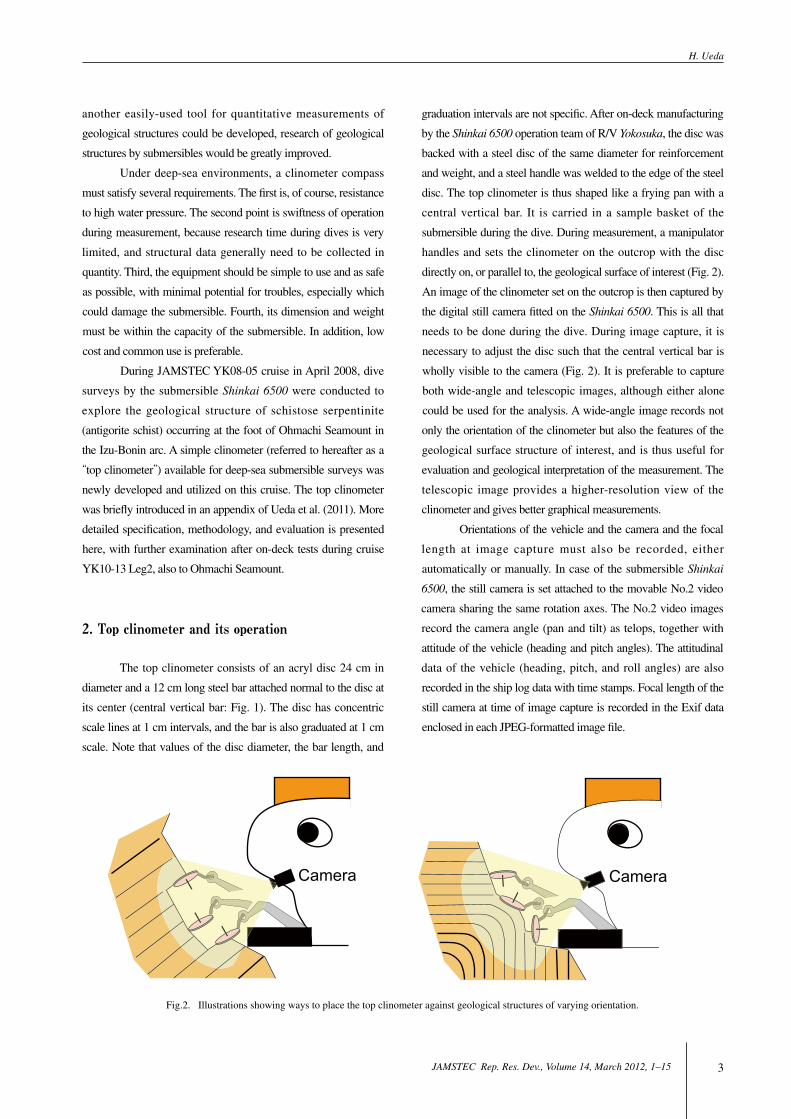
5.4. The angleψTheoretical increments (∆ψ) of the angleψread by the

bar and disc scales (both of 12 graduations) are shown in Fig. 8A.

Increments among 145 possible pairs of the bar-disc scales are not

unique. When the disc is close to the horizontal or vertical, i.e. the

intervals from (b, c) = (0, 12) to (1, 12) and from (12, 0) to (12, 1),

the increment ∆ψis as large as 4-5°. In the remaining range, ∆ψ

values are less than 2.5°. Fig. 8B shows the estimated probabilities

of increments as occupation among the range of 0-90°. Except

for the two large increments close to the horizontal and vertical,

about 95% of the increments are less than 2°. This value is regarded

as the general resolution of the bar-disc scales with 12

graduations. Better resolution can practically be obtained by

reading values of either the bar or the disc to the first decimal

place by eye, even in the intervals of worse resolution, i.e. when

exact overlaps of the integer scales are not found.

The accuracy ofψwas tested in the laboratory by

photographing the variously inclined top clinometer with a

horizontal rotation (Yʼ-) axis normal to the sight line (i.e.ξ is

fixed as 0° ). The top clinometer was photographed at the

approximate center of each picture, and further processed using

the centering correction. In this “dip test”, all dip angles of the disc

are equal to 90° -ψ, and their errors are thus regarded as equivalents

to empirical errors ofψanalysis. Dips of the disc were measured

using a hand clinometer of 1° graduation, and some of the bar-

disc scales were read to the millimeter-scale by eye. This dip test

resulted (Fig. 9) in an excellent 1:1 linear correlation between the

measured and analyzed dips (the correlation coefficient r > 0.99

both for wide-angle and telescopic tests). Errors (2σ ) of the

difference in these measured and analyzed dip values were 0.7°

for wide-angle and 0.4° for the telescopic analyses. To take the

resolution of the hand clinometer into account, these results

suggest that in practice the bar-disc scale method reads the angle

ψas accurately as the hand magnetic clinometer.

5.5. The angle ξBecause the Tx and Ty values obtained from digital images

are integers, increments (∆ξ) exist to determine the angleξ. Fig.

10A shows calculated ∆ξvalues for every given length (lb in px

equivalent) of the measurable part of the bar image. Theoretical Tx

and Ty are given as integer pairs (x, y) nearest to the circle trace of

radius lb, and each neighboring pair provides ∆ξ . The increment

∆ξdepends on the imaged bar length lb, which is a function of

0 10 20 300

10

20

30

Measured angle from camera center (deg)

Analy

zed a

ngle

from

came

ra ce

nter (

deg) 1:1

100 150 200 250 300100

150

200

250

300

6k test (T)6k test (W)Labo. test (T)

Labo. test (W)

Measured distance do (cm)

Analy

zed d

istan

ce do (

cm)

1:1

Fig. 7. A relationship between manually measured and graphically

analyzed centering angles (between the image and disc centers) by a

laboratory test with wide-angle photographs.

Fig. 6. Relationships between manually measured and graphically

analyzed distances do. T: telescopic, and W: wide-angle. In 6k test,

Shinkai 6500 still camera captured the top clinometer placed on the R/V

Yokosuka deck. For laboratory test, see the text.

H. Ueda


distance do, focal length f, and the angleψ . Expected maximum

∆ξvalues (∆ξmax) versus the angleψfor the typical distance do

of 1.5 m and the measurable part of the bar (10 cm), are shown in

Fig. 10B. The ∆ξmax values increase asψapproaches to 0 °.

However, differences of the angleξare less effective on that of

the resultant surface orientation whenψ is small. Therefore, the

effective maximum increment (∆ξmaxsinψ : Fig. 10C) is almost

insensitive to the angle ψ , and is as low as 0.5°, or even less if

wide-angle images are used. These tests suggest that measurement

error for the angleξ is small compared to the other parameters.

Telescopic pictures will provide better results, but wide-angle

images can still be used to determine theξvalues.

5.6. Empirical error of analysis by laboratory testNineteen measurements were made in laboratory tests

capturing images of the top clinometer in varying orientation.

Figs. 11A-B show near 1:1 correlations between manual

measurements by hand magnetic clinometer and graphically

analyzed results from the top clinometer, on dip (inclination) and

azimuth (declination) of pole orientation. Fig. 11C plots

differences between manual measurements and graphical analysis.

Because the accuracy of azimuths depends on correspondent dip,

each difference of azimuths is multiplied by the cosine of

measured dip in this figure to represent the actual effect on the

pole orientation. The 95% probability ellipse for telescopic image

analyses is narrower than that for wide-angle, and the former thus

provides better results. Systematic errors represented by ca. 0.8

and 1.2° shifts of the mean points from the origin for telescopic

and wide-angle analyses, respectively, perhaps resulted from

instrumental errors of the magnetic or top clinometers and/or of

laboratory settings. The long radii of the 95% probable ellipses

were 2.5° for both telescopic and wide-angle analysis, and this can

be regarded as the empirical precision of this test. Because this

value contains errors for the magnetic clinometer, errors of the top

clinometer alone cannot be evaluated in this test. However, it is

probable that accidental errors for the top clinometer itself are less

than ± 2.5° .

6. Calibration for Shinkai 6500

6.1. Flat testDuring the YK08-05 and YK10-13 Leg2 cruises, simple

onboard tests (“flat test”) were made using Shinkai 6500 in R/V

Yokosuka dock. The flat test checks whether the top clinometer

horizontally oriented relative to Shinkai 6500 can be analyzed as

to be horizontal or not. The clinometer was directly placed on the

deck in front of Shinkai 6500 settled on the truck frame, and was

photographed using its still camera. Heading of Shinkai 6500 was

virtually input as 180°. Because the No.2 digital video (DV)

0

10

20

30

40

50

60

70

80

90

0 10 20 30 40 50 60 70 80 90

Analy

zed d

ip (d

eg)

Measured dip (deg)

Wide-angleTelescopic

1:1

Fig. 9. Relationships between manually measured and graphically

analyzed dips in a laboratory “dip test”, when Yʼ axis was fixed

horizontal (ξ= 0°).

0

1

2

3

4

5

6

0 10 20 30 40 50 60 70 80 90Angle between bar and camera center line (ψ deg)

0

20

40

60

80

100

0

10

20

30

40

50

0 1 2 3 4 5

Cumu

lative

prob

abilit

y (%

)

Prob

abilit

y (%

)

Increment of ψ by bar-disc scales (Δψ deg)

Near-horizontal

Near-vertical

Incre

ment

of ψ

by ba

r-disc

scale

s (Δψ

deg)

Fig. 8. Theoretical increments (Δψ) of the angleψ, with twelve

graduations for the bar and disc scales. (A) Distribution of increments

with varying values. (B) Probability (occupation) of increments in the

range of 0-90°.



camera was exchanged for a digital highvision (HDV) camera in

2010 summer, results of the flat tests during these cruises may

represent those for DV and HDV cameras, respectively. The analyzed

strikes and dips were N70 °E12°S in YK08-05 (telescopic),

and N33° E5° E for in YK10-13 Leg2 (only wide-end pictures

were successful) as presented in Table 2. The analyzed dips,

greater than errors for the clinometer itself estimated by laboratory

tests, are probably influenced by the installation of cameras and

their rotation axes on Shinkai 6500. Calibrations were thus made

using still camera images of the flat tests and video movies

captured using Shinkai 6500 on deck. Although calibrations are

indirect and still incomplete, current version of parameter sets

(Table 3) provides better results of the flat test analyses close to

horizontal (Table 2).

0

1

2

3

4

0 10 20 30 40 50 60 70 80 90

Incre

ment

Δξ

(deg

)

ξ (deg)

ψ (deg)

ψ (deg)

lb = 25 px

50

100200400

800

0

5

10

15

20

0 10 20 30 40 50 60 70 80 90

Maxim

um in

crem

ent Δ

ξ max

(deg

)

Δξmax

Δξmax

Δξmax

Δξmax

Camera for labo. testwide-end

tele-endwide-end

tele-endf = 20 mm

f = 35 mm

Shinkai 6500 (6k) still camera

Practical range for 6k still camera

(A)

(B)

(C)

0

0.2

0.4

0.6

0 10 20 30 40 50 60 70 80 90

Δξ m

ax si

nψ (

deg)

-4

-2

0

2

4

-4 -2 0 2 4Difference of analyzed and measured pole azimuths (multiplied by cos(dip), in deg)

Diffe

renc

e of a

nalyz

ed an

d mea

sure

d pole

dips

(deg

)

Telescopic

Wide-angle

Telescopic

Wide-angle

Telescopic

Wide-angle

0

10

20

30

40

50

60

70

80

90

0 10 20 30 40 50 60 70 80 90

Analy

zed p

ole d

ip (to

p clin

omete

r, in

deg)

Measured pole dip (magnetic clinometer compass, in deg)

1:1

180

190

200

210

220

230

240

250

260

270

180 190 200 210 220 230 240 250 260 270

Analy

zed

pole

azim

uth (t

op cl

inome

ter, in

deg)

Measured pole azimuth (magnetic clinometer compass, in deg)

1:1

(A)

(B)

(C)

Fig. 10. (A) Theoretical increments (Δξ) versus the angleξby length

(lb in pixel unit) of measurable parts of the imaged central vertical bar,

with fixed values of do = 150 cm. (B) Maximum increment (Δξmax)

versus the angleψfor varying focal length (also see Table 1).

Measurable part of the bar is fixed as 10 cm. (C) Δξmax sinφvalues

representing actual effect of increments on the surface orientation.

Fig. 11. (A, B) Graphically analyzed dips (inclination) and azimuths

(declination) of pole to variously oriented surfaces compared with

manual measurements by a magnetic hand clinometer. (C) Differences

of measured from analyzed (telescopic) dips and azimuths of poles, with

95% probable ellipses.

H. Ueda


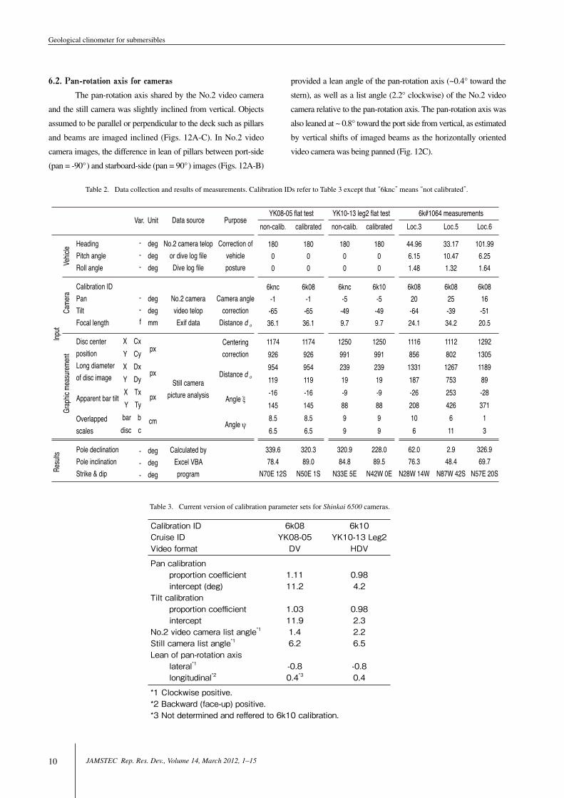
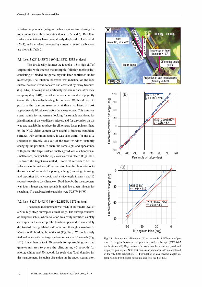
6.2. Pan-rotation axis for camerasThe pan-rotation axis shared by the No.2 video camera

and the still camera was slightly inclined from vertical. Objects

assumed to be parallel or perpendicular to the deck such as pillars

and beams are imaged inclined (Figs. 12A-C). In No.2 video

camera images, the difference in lean of pillars between port-side

(pan = -90°) and starboard-side (pan = 90°) images (Figs. 12A-B)

provided a lean angle of the pan-rotation axis (~0.4° toward the

stern), as well as a list angle (2.2° clockwise) of the No.2 video

camera relative to the pan-rotation axis. The pan-rotation axis was

also leaned at ~ 0.8° toward the port side from vertical, as estimated

by vertical shifts of imaged beams as the horizontally oriented

video camera was being panned (Fig. 12C).

Table 3. Current version of calibration parameter sets for Shinkai 6500 cameras.

CalibrationID 6k08 6k10CruiseID YK08-05 YK10-13Leg2Videoformat DV HDV

Pancalibrationproportioncoefficient 1.11 0.98intercept(deg) 11.2 4.2Tiltcalibrationproportioncoefficient 1.03 0.98intercept 11.9 2.3No.2videocameralistangle*1 1.4 2.2Stillcameralistangle*1 6.2 6.5Leanofpan-rotationaxislateral*1 -0.8 -0.8longitudinal*2 0.4*3 0.4

*1Clockwisepositive.*2Backward(face-up)positive.*3Notdeterminedandrefferedto6k10calibration.

UnitVar.

Input

Resu

ltsVe

hicle

Came

raGr

aphic

mea

surem

ent

HeadingPitch angleRoll angle Calibration IDPanTiltFocal length Disc centerpositionLong diameterof disc image Apparent bar tilt Overlappedscales Pole declinationPole inclinationStrike & dip

---

--f

X CxY CyX DxY DyX TxY Ty

bar bdisc c

---

degdegdeg

degdegmm

px

px

px

cm

degdegdeg

No.2 camera telopor dive log fileDive log file

No.2 cameravideo telopExif data

Still camerapicture analysis

Calculated by

Excel VBAprogram

Correction ofvehicleposture

Camera anglecorrection

Distance d o

Centeringcorrection

Distance d o

Angle ξ

Angle ψ

non-calib. 180

00

6knc-1-6536.1

1174926954119-161458.56.5

339.678.4

N70E 12S

calibrated 180

00

6k08-1-6536.1

1174926954119-161458.56.5

320.389.0

N50E 1S

non-calib. 180

00

6knc-5-499.7

125099123919-98899

320.984.8

N33E 5E

calibrated 180

00

6k10-5-499.7

125099123919-98899

228.089.5

N42W 0E

Loc.3 44.966.151.48

6k0820-6424.1

11168561331187-26208106

62.076.3

N28W 14W

Loc.5 33.1710.471.32

6k0825-3934.2

11128021267753253426

611

2.948.4

N87W 42S

Loc.6 101.99

6.251.64

6k0816-5120.5

12921305118989-28371

13

326.969.7

N57E 20S

Data source PurposeYK08-05 flat test YK10-13 leg2 flat test 6k#1064 measurements

Table 2. Data collection and results of measurements. Calibration IDs refer to Table 3 except that “6knc” means “not calibrated”.



6.3. Still camera installationThe central vertical bar was imaged as nearly vertical by

the No.2 video camera, whereas leaned toward the left-hand side

at 5.4° and 5.7° in the flat test photographs of YK08-05 and

YK10-13, respectively (Fig. 12D). To take the 0.8° lean of the pan-

rotation axis into account, the still camera is presumably installed

listing clockwise by 6.2° and 6.5° clockwise, respectively, relative

to the pan-rotation axis (Table 3).

6.4. Pan and tilt telopsPan angles displayed in video telops were inconsistent

with the inclination of imaged truck frames captured by the

vertically tilted video camera (Fig. 13A). The actual pan angle

assumed from the track frame images are in linear correlations

with correspondent telop values (Fig. 13B), and the correlations

for DV and HDV cameras differ. The installation angles of the

No.2 video camera relative to the pan-rotation axis (1.4° for

YK08-05 and 2.2° for YK10-13 leg2) were subtracted from the

intercepts of the regression formulae to determine the calibration

parameters (Table 3).

Tilt angles were also calibrated in a less accurate but

similar way. The actual vertical direction can be assumed referring

to the projection of the image rotation axis in panned movies

captured by the No.2 video camera facing downward. When the

telop indicates just -90°, the actual tilt angle is estimated by the

differential angle between levels of the image center and the

image rotation axis (Fig. 13A). In near-horizontal images, the

actual horizontal level can be estimated by perspective view

analyses of imaged beams (Fig. 12C). Whereas an apparent

horizontal level based on the telop value is placed at the image

center (or shifted if the telop value is not zero). The differential

angles between the image center level and the estimated horizontal

level provide another constraint. Based on these two controls,

linear formulae were constructed to assume the actual tilt angle

for every given telop value (Fig. 13C).

7. Practical measurements by Shinkai 6500

During 6K#1064 dive (pilot: K. Matsumoto, copilot: K.

Chiba, and scientist: H. Ueda) of the YK08-05 cruise in the

Ohmachi Seamount (Izu-Bonin arc), metamorphic foliation of

2.6o

1.8o

(A)

(B)

(C)

Pan = -90o

Pan = +90o Pan = 0o

Pan-rotation plane

Camera horizontal planeActual horizontal plane(at camera center level)

Difference of telop and actual horizons (2.3o)

Image center

True vertical

Camera horizontal plane

True horizontal plane

-0.8 o

-0.8o Pan-rotation planePan-rotation axis 2.2o: Video camera installation

1.4o

ahead

Camera vertical (+90 o)

True verticalPan axis

2.6o0.4o

Video camerainstallation

2.2o

-1.8o0.4o

Camera vertical (-90 o)

True vertical

Pan axis

Video camerainstallation

2.2oahead

5.7o (D)

No.2 video cameraStill camera

Fig. 12. Calibration for installation of cameras and the pan rotation axis of Shinkai 6500 during YK10-13 Leg2. (A and B): Video clips of lateral

horizontal views by the No.2 video camera (HDV). Insets (with exaggerated angles) are interpretations for leaning of imaged pillars. (C) A frontal and

horizontal view from the No.2 video camera. The pan rotation plane was determined by a vertical shift of an imaged beam in a horizontally panning

movie. Inset shows interpretation of inclination (exaggerated) of the imaged beam and the pan rotation plane. (D) Leaning of the imaged central vertical

bar of the top clinometer on deck captured by the still camera (left) and No.2 video camera (right). In both the images, the clinometer was captured at the

approximate center of the pictures.

H. Ueda


schistose serpentinite (antigorite schist) was measured using the

top clinometer at three localities (Locs. 3, 5, and 6). Resultant

surface orientations have been already displayed in Ueda et al.

(2011), and the values corrected by currently revised calibrations

are shown in Table 2.

7.1. Loc. 3 (29°7.455’N 140°42.193’E, 3333 m deep)This first locality lies neat the foot of a ~15 m high cliff of

serpentinite with intense metamorphic foliation (schistosity)

consisting of bladed antigorite crystals later confirmed under

microscope. The foliation, however, was indistinct on the rock

surface because it was cohesive and cross-cut by many fractures

(Fig. 14A). Looking at an artificially broken surface after rock

sampling (Fig. 14B), the foliation was confirmed to dip gently

toward the submersible heading the northeast. We thus decided to

perform the first measurement at this site. First, it took

approximately 10 minutes before the measurement. This time was

spent mainly for movements looking for suitable positions, for

identification of the candidate surfaces, and for discussion on the

way and availability to place the clinometer. Laser pointers fitted

on the No.2 video camera were useful to indicate candidate

surfaces. For communication, it was also useful for the dive

scientist to directly look out of the front window, instantly

changing the position, to share the same sight and appearance

with pilots. The target surface finally agreed was a subhorizontal

small terrace, on which the top clinometer was placed (Figs. 14C-

D). Since the target was settled, it took 90 seconds to fix the

vehicle onto the outcrop, 45 seconds to place the clinometer onto

the surface, 65 seconds for photographing (centering, focusing,

and capturing two telescopic and a wide-angle images), and 15

seconds to retrieve the clinometer. Total time for the measurement

was four minutes and ten seconds in addition to ten minutes for

searching. The analyzed strike and dip were N28°W 14°W.

7.2. Loc. 5 (29°7.492’N 140°42.2152’E, 3277 m deep)The second measurement was made at the middle level of

a 20 m high steep outcrop on a small ridge. The outcrop consisted

of antigorite schist, whose foliation was easily identified as platy

cleavages on the outcrop. The foliation appeared to moderately

dip toward the right-hand side observed through a window of

Shinkai 6500 heading the northeast (Fig. 14E). We could easily

find and agree with the target surface as quick as 15 seconds (Fig.

14F). Since then, it took 30 seconds for approaching, two and

quarter minutes to place the clinometer, 45 seconds for

photographing, and 50 seconds for retrieving. Total duration for

the measurement, including discussion on the target, was as short

-90

-60

-30

0

30

60

90

120

-90 -60 -30 0 30 60 90 120

Grap

hicall

y esti

mated

pan a

ngle

(deg

)

Pan angle on telop (deg)

-90

-60

-30

0

-90 -60 -30 0

Grap

hicall

y esti

mated

tilt a

nge (

deg)

Tilt angle on telop (deg)

YK10-13 Leg2 (HDV)y = 0.98x + 2.3

YK10-13 Leg2 (HDV)y = 0.98x + 6.4

YK08-05 (DV)y = 1.03x + 11.9

YK08-05 (DV)y = 1.11x + 12.6

(B)

(C)

Image center level(Telop tilt = -90o)

Truck frame

Telop:pan = 97o, tilt = -90o

Differential angle(9.0o)

(A)

YK08-05

Actual 90 o direction

Actual 97 o direction Telop pan = 97 o

Projection of pan- rotation axis(Actually vertical)

Fig. 13. Pan and tilt calibrations. (A) An example of difference of pan

and tilt angles between telop values and an image (YK08-05

calibration). (B) Regression of correlation between analyzed and

displayed pan angles. Note that non-linear plots near -90° are excluded

in the YK08-05 calibration. (C) Formulation of analyzed tilt angles vs.

telop values. For the near-horizontal analysis, see Fig. 12C.



as five minutes. The resultant strike and dip were analyzed as

N87°W 42°S.

7.3. Loc. 6 (29°7.4097’N 140°42.3217’E, 3259 m deep)This locality is one of the outcrops sporadically exposed

on a steep slope. The outcrop was a 4-5 m high cliff surrounded

by talus deposits. Foliation was partly obvious and appeared

gently dipping beyond and righthand side observed from the

submersible heading the east. It was, however, crosscut by many

vertical joints (Fig. 14G). Some of foliation planes and joints were

open, and the rock was loose and fragile. The orientation of the

foliation could thus be modified by creep movements, and caution

must be paid for geological interpretation of the result. However,

it does not matter to test the methodology.

In this measurement, the operator placed the top

clinometer so as to extend a platy foliation without any direction

by the scientist (Fig. 14H). It took two and half minutes, including

a time for approaching to the outcrop. Then, it took one minute for

checking and acceptance by the scientist, one minute and ten

seconds for photographing, and 35 seconds for retrieving. Totally,

the measurement was completed for five minutes and ten seconds.

Because of light scattering owing to stirred mud, the obtained

image were overexposed (Fig. 14H). Graphic retouching

fortunately enabled to read bar and disc scales (Fig. 14I).

(A)

Loc. 3 Loc. 3

(C)

Loc. 5

(E)

Loc. 5

(F)

Loc. 6

(H)(G)

Loc. 6 Loc. 6

Loc. 3

(D)

Loc. 3

(B)

(I)

Fig. 14. Outcrop features and measurements of serpentinite foliation using the top clinometer during 6K#1064 dive in YK08-05 cruise. (A-D) Loc. 3: (A)

Blocky rock surfaces with indistinct foliation. Measured part is on the right extension of the picture. (B) Pale foliation surface appeared on an artificially

broken part after sampling (arrow). Measured part is ~1 m above the picture. (C): Captured No.2 video image at the measurement. (D) Close-up still

camera picture used for analysis. Black arrow indicates the bar-disc scale overlap, and yellow arrows indicate fractures along with foliation planes. (E and

F) Loc. 5: (E) Distinctly foliated rock surface. Measurement was made on the lower-left extension of this picture. (F) Captured No.2 video image at the

measurement. For correspondent still camera view, see Fig. 5. (G-I) Loc. 6: (G) Fractured rock surfaces with foliation crosscut by vertical joints.

Measurement point is on the upper-right extension of this picture. (G) Captured No.2 video image of the measurement against loose foliation planes. (H)

The close-up picture of the measurement, with retouched version as inset. The accepted bar-disc scale overlap is shown by arrows.

H. Ueda


8. Availability and problems

As noted in the section of introduction, a clinometer for

deep-sea measurements requires (1) resistance to water pressure,

(2) swiftness of operation, (3) simple and safe, and (4) minimal

size and weight, in addition to general requirement of (5) cost and

(6) data reliability. Among these, the top clinometer evidently

satisfies (1) resistance, (3) safety, (4) size and weight, and (5) cost.

Theoretical and laboratory tests evaluated that the top

clinometer itself can measure as precise as magnetic clinometer

compasses commonly used on-land. It also has an advantage of

independence from magnetic fields, which can be affected by the

submersible and strongly magnetized rocks. However, its data

reliability depends significantly on camera installation on

submersibles. The present calibration parameters were determined

by indirect and inferable information such as assumingly vertical

and horizontal objects in pictures. Although they seemingly

provided valid results by on-deck flat test, the examined

orientation was very limited (unity) and thus may not be sufficient

for the multi-parameter calibration. More directly measured

parameters and examination on more variously oriented top

clinometer will improve its reliability. In addition, cameras and

their rotation axes equipped on the submersible Shinkai 6500 are

removed and re-installed at every (mainly annual) opportunity of

maintenance in dock. Therefore, it is preferable to calibrate and to

perform on-deck test at least once in every year.

The time necessary for a measurement was as short as

five minutes. And there has been no technical problem of

operation. The measurement itself is thus evaluated to be simple

and quick enough. However, the actual time could be much

expended to look for a target surface and to communicate about

position and the way to place the clinometer. It is important for a

dive scientist to choose sites with simple and easy surfaces, as

possible, for operators to recognize and to place the clinometer.

So far there are two major problems to be improved in

future. First, the top clinometer of the current version tends to be

pictured with overexposure, especially at flat test on deck and at

seafloor when water is stirred with mud. It probably owes to

coloring of the current top clinometer: white and yellow parts of

the disc and bar, respectively, might be sometimes too bright

compared to backgrounds, or scattered light could enhance

brightness of these parts, which may not be concerned by the

exposure meter. Graphical retouching can overcome this problem

in fortunate cases (Figs. 14H and 14I). However, extreme

overexposure disables to correctly read the disc-bar scales:

brightly colored graduations invade dark-colored ones. Therefore,

reexamination of coloring is necessary for stably successful

measurements. Second, the central vertical bar can be stuck in the

sample basket and bent out of vertical. The bar is easily replaced

with a spare on deck. However, when it happens on seafloor, it

will be difficult to continue valid measurements during the rest

time of the dive. Hence, mechanical improvements increasing

toughness or protecting the bar is also necessary.

Finally I note that the top clinometer is available on

request.

Acknowledgments

This work arose from discussions with Drs. K. Kizaki and

T. Shimura, who had ideas of universal magnetic clinometers of

very easy use. Mr. T. Yoshiume kindly provided basic information

on camera specifications and installations on the submersible

Shinkai 6500, based on which the current idea of the clinometer

developed and realized. Laboratory tests were accomplished by

assistance of Mr. T. Saito. The clinometer would not reach to the

level of practical use without on-deck manufacturing by the

Shinkai 6500 operation team during YK08-05 cruise. Pilots and

dive scientists of YK08-05, YK10-04, and YK10-13 Leg2 all

equipped it at their dives, and Drs. K. Hirauchi, M. Meschede, and

K. Tani made measurements in their dives. These precious

experiences were not described in the text but implicitly

contributed to confirm its availability. Dr. B. P. Roser kindly made

corrections on language. Peer reviews by Drs. R. Anma and K.

Kawamura and editorial reviews by Dr. T. Miyazaki significantly

improved the manuscript. This work was financially supported by

JSPS Grant-in-Aid no. 22540464. I appreciate these persons and

organizations.

References

Anma, R., Y. Ogawa, K. Kawamura, G. Moore, T. Sasaki, S.

Kawakami, S. Hirano, T. Ota, R. Endo Y. Michiguchi,

and YK05-08 Shipboard Science Party (2010), Structure,

texture, and physical properties of accretionary prism

sediments and fluid flow near the splay fault zone in the

Nankai Trough, off Kii Peninsula. J. Geol. Soc. Japan,

116, 637-660.

Cogné, J. P., J. Francheteau, V. Courtillot and Pito93 Scientific

Team (1995), Large rotation of the Easter microplate as

evidenced by oriented paleomagnetic samples from the



ocean floor. Earth Planet. Sci. Lett., 136, 213-222.

Hurst, S. D., J. A. Karson, and K. L. Verosub (1994),

Paleomagnetic study of tilted diabase dikes in fastspread

oceanic crust exposed at Hess Deep. Tectonics, 13, 789-

802.

Karson, J. A., G. L. Früh-Green, D. S. Kelley, E. A. Williams, D.

R. Yoerger, and M. Jakuba (2006), Detachment shear

zone of the Atlantis Massif core complex, Mid-Atlantic

Ridge, 30N. Geochem. Geophys. Geosyst., 7, Q06016,

doi:10.1029/2005GC001109.

Kocak, D. M., F. M. Caimi, P. S. Das, and J. A. Karson (1999),

A 3-D laser line scanner for outcrop scale studies of

seafloor features, Proceedings OCEANS '99 MTS/IEEE

“Riding the Crest into the 21st Century”, 3, 1105- 1114.

Lawrence, R. M., J. A. Karson and S. D. Hurst (1998), Dike

orientations, fault-block rotations, and the construction of

slow spreading oceanic crust at 22°40ʼN on the Mid-

Atlantic Ridge. J. Geophys. Res., 103, 663-676.

Ogawa, Y., K. Kobayashi, H. Hotta, and K. Fujioka (1997),

Tension cracks on the oceanward slopes of the northern

Japan and Mariana Trenches. Marine Geol., 141, 111-

123.

Ueda, H., K. Niida, T. Usuki, K. Hirauchi, M. Meschede, R.

Miura, Y. Ogawa, M. Yuasa, I. Sakamoto, T. Chiba, T.

Izumino, Y. Kuramoto, T. Azuma, T. Takeshita, T.

Imayama, Y. Miyajima, and T. Saito (2011), Seafloor

geology of the basement serpentinite body in the

Ohmachi Seamount (Izu-Bonin arc) as exhumed parts of

a subduction zone within the Philippine Sea, Ogawa, Y.,

R. Anma and Y. Dilek (eds.), Accretionary Prisms and

Convergent Margin Tectonics in the Northwest Pacific

Basin, Springer, 97-128.

H. Ueda


Documents

Sea-floor in situ measurement of orientation of geological ...€¦ · Sea-floor in situ measurement of orientation of geological structures using a ... Theoretical and laboratory