Sea-spike Detection in High Grazing Angle X-band Sea-Clutter · UNCLASSIFIED Sea-Spike Detection in High Grazing Angle X-band Sea-Clutter Luke Rosenberg Electronic Warfare and Radar

UNCLASSIFIED

Sea-Spike Detection in High Grazing Angle X-bandSea-Clutter

Luke Rosenberg

Electronic Warfare and Radar Division

Defence Science and Technology Organisation

DSTO–TR–2820

ABSTRACT

Knowledge of radar sea-clutter phenomenology allows accurate models to be devel-oped for assessing target detection performance. The majority of work in this area hasbeen at low-grazing angles from clifftops or wave tanks and does not consider scat-tering in the high grazing angle region beyond 10◦. To improve our understandingat high grazing angles 15◦ to 45◦, the DSTO’s Ingara airborne X-band fully polari-metric radar has been used to collect 12 days worth of sea-clutter data. This reportfocuses on understanding the characteristics of sea-spikes as they are often the causeof false detections in a radar processor. Using the Ingara data, a threshold is used toisolate these scatterers in the range/time domain with results verified against the KKprobability distribution function. Detections due to discrete and persistent scatteringare then isolated to provide more information regarding the underlying cause of sea-spikes and answer the question of whether Walker’s three component mean Dopplerspectrum model is suitable at high grazing angles.

APPROVED FOR PUBLIC RELEASE

UNCLASSIFIED

DSTO–TR–2820 UNCLASSIFIED

Published by

DSTO Defence Science and Technology OrganisationPO Box 1500Edinburgh, South Australia 5111, Australia

Telephone: (08) 7389 5555Facsimile: (08) 7389 6567

c© Commonwealth of Australia 2013AR No. 015-571April 2012

APPROVED FOR PUBLIC RELEASE

ii UNCLASSIFIED

UNCLASSIFIED DSTO–TR–2820

Sea-Spike Detection in High Grazing Angle X-band Sea-Clutter

Executive Summary

This report builds on work undertaken at the Defence Science and Technology Organisation(DSTO) in characterising the maritime environment from high altitude airborne platforms. Tradi-tionally, maritime surveillance of small targets is conducted from low altitude platforms and hencewith low grazing angles. This surveillance scenario has been well studied and relevant modelshave been developed. However, little data has been collected and analysed from the high grazingangles typically expected with the operation of high altitude airborne platforms. In August 2004and July 2006, the DSTO’s Ingara X-band airborne radar collected fine resolution fully polarimet-ric data in the high grazing angle region, 15◦ − 45◦. The data was collected in the ocean off thecoasts of Port Lincoln and Darwin respectively.

This report investigates the detection and characterisation of sea-spikes which result from non-Bragg scattering with the goal of being able to better distinguish them from targets of interest. Theapproach taken is to threshold the magnitude of the raw backscatter data in the range/time domain.The percentage of sea-spikes present in the data is then measured. Results show that the majorityoccur in the lower grazing angle region for the horizontal transmit, horizontal receive (HH) channeland are slightly higher in the cross wind directions for the horizontal transmit, vertical receive (HV)and vertical transmit, vertical receive (VV) channels. These results are verified by comparing thetrends with a separate analysis which used the KK probability distribution function (PDF) to modelthe sea-clutter.

An image processing algorithm is then used to isolate the discrete and persistent scatterers andtest whether Walker’s mean Doppler spectrum model is valid with the higher grazing angles. Theresults show that the persistent ‘whitecaps’ are spread quite evenly in grazing and azimuth for theHH channel with a clear trend in the cross-wind directions for the HV and VV channels. Whilethere were many common peaks in both the HH and VV channels, there are however, a lot ofdetections present in HH but not in VV. Also, there are many discrete scatterers detected in theVV channel. This indicates that Walker’s three channel model is not totally valid at high grazingangles.

UNCLASSIFIED iii


THIS PAGE IS INTENTIONALLY BLANK

iv UNCLASSIFIED


Author

Dr. Luke RosenbergElectronic Warfare and Radar Division

Luke Rosenberg received his BE (Elec.) with Honours from Ade-laide University in 1999 and joined DSTO in January 2000. Sincethis time he has completed both a Masters degree in signal and in-formation processing and a PhD in multichannel synthetic apertureradar through Adelaide University. He has worked at the DSTO asan RF engineer in the Missile Simulation Centre, as a Research Sci-entist in the imaging radar systems group and now in the MaritimeRadar Group. Current research interests include radar and cluttermodelling, adaptive filtering and radar detection theory.

UNCLASSIFIED v


THIS PAGE IS INTENTIONALLY BLANK

vi UNCLASSIFIED


Contents

1 Introduction 1

2 Background 2

2.1 Sea-spike discrimination . . . . . . . . . . . . . . . . . . . . . . . . . . . . . 2

2.2 Radar description and pre-processing . . . . . . . . . . . . . . . . . . . . . . 4

2.3 Trials background . . . . . . . . . . . . . . . . . . . . . . . . . . . . . . . . . 4

3 Sea-spike analysis 7

3.1 Sea-spike detection . . . . . . . . . . . . . . . . . . . . . . . . . . . . . . . . 7

3.2 Probability distribution . . . . . . . . . . . . . . . . . . . . . . . . . . . . . . 7

3.3 Persistent and discrete detections . . . . . . . . . . . . . . . . . . . . . . . . . 9

3.4 Sea-spike characteristics . . . . . . . . . . . . . . . . . . . . . . . . . . . . . 15

3.5 Doppler spectrum . . . . . . . . . . . . . . . . . . . . . . . . . . . . . . . . . 18

4 Conclusion 20

References 21

UNCLASSIFIED vii


Figures

1 Ingara pre-processing diagram . . . . . . . . . . . . . . . . . . . . . . . . . . . . 5

2 Circular spotlight mode collection geometry . . . . . . . . . . . . . . . . . . . . . 6

3 Percentage of sea-spike detections . . . . . . . . . . . . . . . . . . . . . . . . . . 8

4 PDF example . . . . . . . . . . . . . . . . . . . . . . . . . . . . . . . . . . . . . 9

5 Ratio of means from the KK-distribution . . . . . . . . . . . . . . . . . . . . . . . 10

6 Line detection algorithm overview . . . . . . . . . . . . . . . . . . . . . . . . . . 10

7 Thresholded data and line detection example stages 1 and 2 . . . . . . . . . . . . . 11

8 Dominant line detection example . . . . . . . . . . . . . . . . . . . . . . . . . . . 12

9 Clean line detection example . . . . . . . . . . . . . . . . . . . . . . . . . . . . . 12

10 Merged line detection example . . . . . . . . . . . . . . . . . . . . . . . . . . . . 13

11 Percentage of whitecap detections . . . . . . . . . . . . . . . . . . . . . . . . . . 14

12 Percentage of discrete sea-spike detections . . . . . . . . . . . . . . . . . . . . . . 14

13 F35 sea-spike characteristic PDFs - wave velocity, life time and decorrelation time . 16

14 F9 sea-spike characteristic PDFs - wave velocity, life time and decorrelation time . 16

15 F35 sea-spike characteristic PDFs - persistent and discrete magnitudes . . . . . . . 17

16 F35 sea-spike characteristic PDFs - persistent and discrete magnitudes . . . . . . . 17

17 Dual-pol sea-spike example . . . . . . . . . . . . . . . . . . . . . . . . . . . . . . 19

Tables

1 Standard radar operating parameters for ocean backscatter collections . . . . . . . 4

2 Wind and wave ground truth . . . . . . . . . . . . . . . . . . . . . . . . . . . . . 6

3 F35 sea-spike characteristic means . . . . . . . . . . . . . . . . . . . . . . . . . . 15

4 F9 sea-spike characteristic means . . . . . . . . . . . . . . . . . . . . . . . . . . . 15

viii UNCLASSIFIED


1 Introduction

In August 2004 and July 2006, the DSTO Ingara X-band airborne Synthetic Aperture Radar (SAR)collected fine resolution dual and fully polarimetric data over the high grazing angle region, 15◦ to45◦. This report builds on work undertaken at the DSTO to understand the characteristics of sea-clutter in order to validate existing and formulate new statistical models for the sea-clutter. Thesestudies have included the mean backscatter, amplitude statistics and the mean Doppler spectrum[Crisp et al. 2008, Dong 2006, Rosenberg, Crisp & Stacy 2010, Rosenberg & Stacy 2008, Rosen-berg, Crisp & Stacy 2008]. This report focuses on the detection and characterisation of the sea-spike component of sea-clutter with the goal of being able to better distinguish them from targetsof interest.

There are three main methods of characterising the sea-spike component of the sea-clutter.The first is to apply a threshold to the data in order to distinguish between Bragg scattering andsea-spike events [Jessup, Melville & Keller 1991, Liu & Frasier 1998, Melief et al. 2006, Walker2001b]. This is done without any assumption about the underlying statistics. The second and thirdmethods fit relevant models to the PDF and the mean Doppler spectrum respectively, [Dong 2006,Rosenberg, Crisp & Stacy 2010, Walker 2001a, Rosenberg & Stacy 2008, Rosenberg, Crisp &Stacy 2008]. These models incorporate parameters to distinguish between the different scatteringmechanisms present in the sea-clutter.

This report uses the first method in order to test the validity of relevant PDF and mean Dopplerspectrum models. Section 2 describes the different scattering components present in sea-clutterand a review of techniques which have been applied to distinguish between them. Also included inthis section is relevant background on the Ingara radar and details of the sea-clutter trials. Section3 then presents a methodology for detecting sea-spikes with a suitable threshold. Comparisonsare made with the KK PDF model [Dong 2006, Rosenberg, Crisp & Stacy 2010] as a means ofverifying the results.

The most relevant mean Doppler spectrum model is based on data from low grazing angles[Walker 2001a]. Walker has proposed a three element model for Bragg, persistent whitecapand discrete sea-spike scattering. In this two channel model (HH and VV), the persistent white-cap components are common in both channels, while the ‘discrete’ sea-spike component is onlypresent in HH. This model has been applied to the Ingara data [Rosenberg & Stacy 2008, Rosen-berg, Crisp & Stacy 2008] but the question was raised whether this model was appropriate athigher grazing angles. Unfortunately, due to the low pulse repetition frequency (PRF) of the full-pol Ingara data, it is not easy to distinguish the three separate components in the Doppler spectrum.Further processing in the range/time domain is therefore applied to identify persistent sea-spikescorresponding to wave crests or ‘whitecaps’. The relationship between the persistent sea-spikesand the mean Doppler spectrum is shown with a description of Walker’s three component Dopplerspectrum model. The new results are then used to assess the validity of this model at high grazingangles.

UNCLASSIFIED 1


2 Background

There are a number of textbooks which focus on aspects of modelling sea-clutter, [Skolnik 1990,Nathanson, Reilly & Cohen 1991, Long 2001, Ward, Tough & Watts 2006]. The first two sum-marise early work from the 1960s and 1970s with a useful summary of sea-clutter radar crosssection (RCS) values up to 60◦ grazing in [Nathanson, Reilly & Cohen 1991]. Long [2001] aswell as discussing this early work with detailed notes on the literature, goes on to more recentwork, such as [Lee et al. 1995b], which considers higher grazing angles.

Section 2.1 describes the different scattering components present in sea-clutter and a review oftechniques which have been applied to distinguish between them. A brief description of the Ingararadar is then presented in Section 2.2 with background to the two sea-clutter trials presented inSection 2.3.

2.1 Sea-spike discrimination

Sea-clutter was originally characterised by matching experimental data with a combination of elec-tromagnetic and rough surface scattering theory. The ‘composite surface model’ was originallyproposed to describe this Bragg scattering theory [Wright 1968, Peake 1959]. Further researchthen led to hydrodynamic models which were used to explain the physical nature of the waves andshowed a good match with the existing theory [Valenzuela & Laing 1970]. However, as more ex-perimental data was collected, it was found that larger wind speeds caused waves which travelledat faster speeds than was predicted by the Bragg theory.

Over the past years, a number of authors have proposed different theories to explain the seadynamics due to non-Bragg scattering, [Duncan, Keller & Wright 1974, Jessup, Keller & Melville1990, Jessup, Melville & Keller 1991, Werle 1995, Lee et al. 1995a, Keller, Gotwols & Chapman2002, Melief et al. 2006]. These are primarily concerned with analysis of breaking waves andunderstanding the main components of the associated radar response. Non-Bragg scattering iscommonly represented as a single component and referred to as ‘sea-spikes’. A common definitionof a sea-spike is a radar return which has a large Doppler component with a wide bandwidth, strongbackscatter power as well as a HH return that is equal or greater than the VV return. Lee et al.[1995a] summarises three possibilities to explain the phenomena which contribute to non-Braggscattering:

• There is a wave which is about to break and has a much longer wavelength than the Braggresonant wave.

• There is a breaking wave which has a long wavelength and large specular return.

• There is an attenuation in the VV channel due to Brewster angle damping and the HHchannel is affected by multipath scattering and shadowing of the wave troughs by largecrests.

Alternatively, Long [2001] has distinguished sea-spikes by their duration, with some lasting for ashort time before fading rapidly and others persisting for 1-2 seconds. These second type are whatare commonly mistaken for targets as they may exhibit many of the same characteristics includingpolarisation independence.

2 UNCLASSIFIED


There have been a number of techniques proposed for discriminating between different typesof scattering by thresholding the data. The first significant study was by Jessup, Melville & Keller[1991] who looked closely at the relationship between breaking waves and sea-spikes. An exper-iment was conducted on a platform in the Chesapeake Bay using a Ku band scatterometer with a45◦ grazing angle. By analysing a 15 s block of data, the frequency spectrum was calculated every0.25 s and the two-dimensional spectrogram was analysed. At points where breaking waves wereobserved, the HH to VV ratio was close to unity, the sea-spike backscatter maxima occurred closein time to local maxima in the mean Doppler frequency and the bandwidth maxima associated withthe sea-spikes was delayed from the sea-spike maxima by approximately 0.25-0.5 s. After carefulanalysis of each wave using a video camera, it was found that 80% of the sea-spike events weretypically associated with breaking waves and could be tracked for seconds in the field of view ofthe radar or up to 5 metres downwind of the breaking wave. A number of criteria were then usedfor detecting sea-spikes caused by breaking waves. These were based on an arbitrary RCS thresh-old applied to each polarisation channel, a threshold applied to the bandwidth and a combinationof both. It was found that the latter threshold achieved a detection rate of approximately 70% withsimilar results for both polarisation channels.

A related study by Keller, Gotwols & Chapman [2002] used the same scatterometer as Jessup.To detect sea-spikes, they used the same combined criteria with the added conditions that thebackscatter power must exceed the mean for at least a second and the Doppler bandwidth mustpeak within that time window. They verified their results using co-located video and looked atdifferent grazing angles, wind speeds and directions. One interesting result from their study wasthat as the grazing angle decreased below 30◦, the VV spikes became more common than HH.

A similar study was conducted with lower grazing angles at X-band by Liu & Frasier [1998].They also used a video camera to distinguish between sea-spikes caused by steep sloping wavesand those from breaking whitecaps. They estimated the magnitude, velocity and coherence of thedual-pol data they received for four different sea conditions. Their criteria for detecting sea-spikesis a power level 10 dB above the mean noise plus clutter level, combined with a coherence whichexceeds 0.8. Their analysis also looked at the Doppler spectrum and found that the majority ofsea-spikes have a HH to VV ratio above unity. They conclude that it is difficult to distinguishbetween the different sea-spike mechanisms and that a simpler criterion based solely on the powerthreshold should be sufficient to detect sea-spikes.

This was the approach taken by Melief et al. [2006] who looked at low grazing angle clifftopdata and observed that the spiking events associated with breaking waves possess a HH powerwhich is equal or higher than their power in the VV channel. By looking at the ratio of HH to VVand the Doppler frequency as a function of range and time, a threshold criterion was developed,p > µ+ nσ, where µ and σ are the the mean and standard deviation of the backscatter magnitudeand n is a positive number. They found a wide spread of values in the sea-spike density as it variedwith grazing, azimuth and wind speed.

Another technique is to apply a low pass filter to the data [Walker 2001b]. Walker demon-strated that with an appropriate choice of cutoff frequency, it is possible to separate sea-spikesfrom the sea-clutter. The study by Dong & Crisp [2008] has looked at the application of the Eulerdecomposition to high grazing angle X-band sea-clutter. They discriminated sea-spikes by takingthe top 0.1% of the highest RCS reflectivity from either the HH or VV channel. Interestingly withthis criterion, 98% of the sea-spikes belonged to the VV channel.

Finally, the paper by Greco, Stinco & Gini [2010] looked at identifying sea-spikes from a

UNCLASSIFIED 3


fixed X-band radar for HH and VV channels independently and then combined together. Theirclassification metric comprises a minimum spike width of 0.1 s, a minimum interval betweenspikes of 0.5 s and a power criterion where the amplitude is five times the mean power of thereceived returns.

2.2 Radar description and pre-processing

The DSTO Ingara system is an airborne multi-mode X-band imaging radar system. It operateswith a centre frequency of 10.1 GHz and supports a 600 MHz bandwidth for fine resolution in aspotlight mode. The sea-clutter trials however used a bandwidth of 200 MHz to achieve a largerswath width. The radar is fully polarimetric and utilises a dual linear polarised antenna developedby the Australian CSIRO for both transmitting and receiving [Parfitt & Nikolic 2001]. In fullypolarimetric collections, the system is operated at double the normal PRF with the polarisationswitch used to alternate the transmit polarisation between horizontal and vertical polarisationswhile receiving horizontal and vertical polarisations simultaneously. A more detailed descriptionof the system may be found in [Stacy et al. 2003]. The standard radar operating parameters usedduring the sea-clutter collections are shown in Table 1. Note that the azimuth resolution is coarsesince the radar is operated in a real beam mode.

Table 1: Standard radar operating parameters for ocean backscatter collections

Parameter ValueFrequency 10.1 GHzTransmitted bandwidth 200 MHzRange / az. resolution 0.75 m / 63 mSpecified pulse separation 0.15 mFull-pol. pulse separation 0.30 m

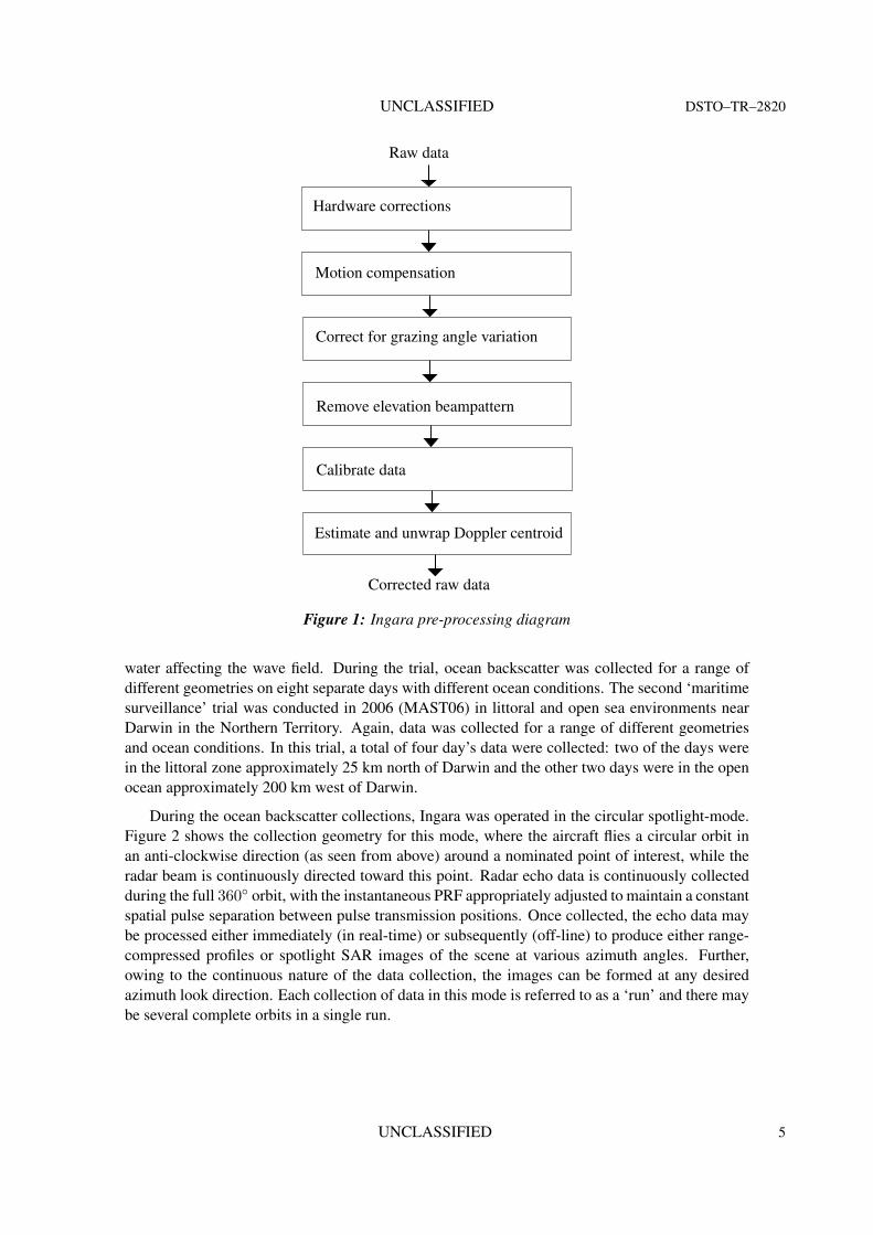
Before the data was analysed, a number of pre-processing steps were applied. Firstly, to avoidbiasing the results, the data set was scanned to identify and remove any ‘bad’ regions. Theseinclude some transmit-off regions which were sampled and any other artifacts due to the radarcollection. This was done visually and less than 1% of data was removed in this way. The rawdata then goes through the processing chain shown in Figure 1. Range processing occurs in hard-ware as a stretch process. The sampled signal was then processed to first remove bandpass filtermodulations and adjusted for motion compensation using both the inertial navigation unit and theglobal positioning system onboard the radar platform. The next steps included a correction forthe variation in ground range resolution due to changes in grazing angle, removal of the elevationbeampattern and polarimetric calibration using the procedure described in [Quegan 1994].

2.3 Trials background

The trial data was obtained with Ingara on two separate occasions and from two distinctly differentregions. The first ‘sea-clutter’ trial was conducted in 2004 (SCT04) in the southern ocean approxi-mately 100 km south of Port Lincoln, South Australia [Crisp, Stacy & Goh 2006]. The site chosenwas at the edge of the South Australian continental shelf where there was little chance of shallow

4 UNCLASSIFIED


Raw data

Hardware corrections

Motion compensation

Remove elevation beampattern

Calibrate data

Corrected raw data

Estimate and unwrap Doppler centroid

Correct for grazing angle variation

Figure 1: Ingara pre-processing diagram

water affecting the wave field. During the trial, ocean backscatter was collected for a range ofdifferent geometries on eight separate days with different ocean conditions. The second ‘maritimesurveillance’ trial was conducted in 2006 (MAST06) in littoral and open sea environments nearDarwin in the Northern Territory. Again, data was collected for a range of different geometriesand ocean conditions. In this trial, a total of four day’s data were collected: two of the days werein the littoral zone approximately 25 km north of Darwin and the other two days were in the openocean approximately 200 km west of Darwin.

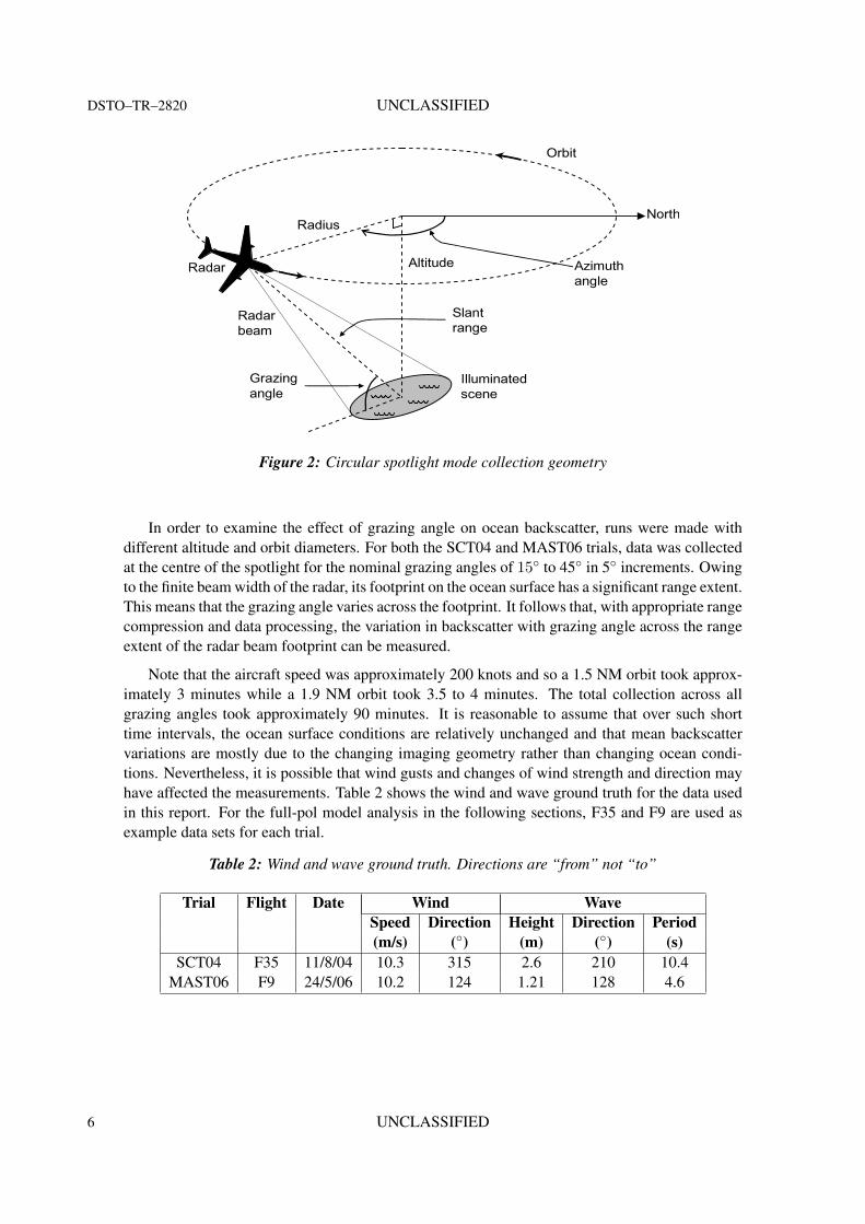
During the ocean backscatter collections, Ingara was operated in the circular spotlight-mode.Figure 2 shows the collection geometry for this mode, where the aircraft flies a circular orbit inan anti-clockwise direction (as seen from above) around a nominated point of interest, while theradar beam is continuously directed toward this point. Radar echo data is continuously collectedduring the full 360◦ orbit, with the instantaneous PRF appropriately adjusted to maintain a constantspatial pulse separation between pulse transmission positions. Once collected, the echo data maybe processed either immediately (in real-time) or subsequently (off-line) to produce either range-compressed profiles or spotlight SAR images of the scene at various azimuth angles. Further,owing to the continuous nature of the data collection, the images can be formed at any desiredazimuth look direction. Each collection of data in this mode is referred to as a ‘run’ and there maybe several complete orbits in a single run.

UNCLASSIFIED 5


Figure 2: Circular spotlight mode collection geometry

In order to examine the effect of grazing angle on ocean backscatter, runs were made withdifferent altitude and orbit diameters. For both the SCT04 and MAST06 trials, data was collectedat the centre of the spotlight for the nominal grazing angles of 15◦ to 45◦ in 5◦ increments. Owingto the finite beam width of the radar, its footprint on the ocean surface has a significant range extent.This means that the grazing angle varies across the footprint. It follows that, with appropriate rangecompression and data processing, the variation in backscatter with grazing angle across the rangeextent of the radar beam footprint can be measured.

Note that the aircraft speed was approximately 200 knots and so a 1.5 NM orbit took approx-imately 3 minutes while a 1.9 NM orbit took 3.5 to 4 minutes. The total collection across allgrazing angles took approximately 90 minutes. It is reasonable to assume that over such shorttime intervals, the ocean surface conditions are relatively unchanged and that mean backscattervariations are mostly due to the changing imaging geometry rather than changing ocean condi-tions. Nevertheless, it is possible that wind gusts and changes of wind strength and direction mayhave affected the measurements. Table 2 shows the wind and wave ground truth for the data usedin this report. For the full-pol model analysis in the following sections, F35 and F9 are used asexample data sets for each trial.

Table 2: Wind and wave ground truth. Directions are “from” not “to”

Trial Flight Date Wind WaveSpeed Direction Height Direction Period(m/s) (◦) (m) (◦) (s)

SCT04 F35 11/8/04 10.3 315 2.6 210 10.4MAST06 F9 24/5/06 10.2 124 1.21 128 4.6

6 UNCLASSIFIED


3 Sea-spike analysis

Sea-spike detection is now performed using two days from the Ingara data set, one from the south-ern ocean near Port Lincoln and the other in the open ocean near Darwin. These are described inTable 2 as F35 and F9 respectively. For the results in this report, the upwind direction (wind to-wards the radar) is rotated to 0◦ with the downwind direction at−180◦, the crosswind directions at±90◦ and any regions with poor or missing data are shown with cross-hatching (diagonal stripes).

Section 3.1 describes the percentage of sea-spikes which are measured after applying a suitablethreshold. Comparison with the KK PDF model is then presented in Section 3.2. The next Section3.3 presents a method for discriminating between the discrete and persistent sea-spikes in the sea-clutter. Further characterisation of the sea-spikes is then presented in Section 3.4. This is followedby Section 3.5 which looks at the relationship between the sea-spike components and the meanDoppler spectrum. Results from throughout this section are then used to assess the validity ofWalker’s three component Doppler spectrum model at high grazing angles.

3.1 Sea-spike detection

To separate the sea-spike components, each run is split into blocks covering 1 degree in grazingand 5 degrees in azimuth. Each block then has an overlap region to allow for the detection ofpersistent spikes which lie in the final second of the data block. Since each data block spans adifferent azimuth and grazing region, a weighted average was determined by the amount of thedata block which falls into the defined grid. From a study of the literature, the criterion by Meliefet al. [2006] was applied to the backscatter magnitude. After careful analysis of our data, a valueof n = 5 standard deviations above the mean was chosen for the threshold. This choice clearlypicked up both the discrete spikes and persistent detections. The thresholded data can then beanalysed to calculate the percentage of detections against the total number of pixels in the image.

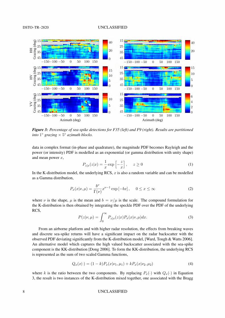
With this threshold, the false alarm rate for F35 was calculated to be 2.8 × 10−3, 8.1 × 10−4

and 3.8 × 10−4 for the HH, HV and VV channels respectively. Similarly for F9, the false alarmrate was calculated as 2.5×10−3, 7.9×10−4 and 3.1×10−4. The first result in Figure 3 shows thepercentage of sea-spike detections against the total number of points. For both data sets, there aremore sea-spike detections in the HH channel than the VV and the majority of sea-spike detectionsoccur in the lower grazing angle region for the HH channel. They are also slightly higher in thecrosswind directions for the other two polarisation channels. Other minor differences are due tothe different sea conditions.

3.2 Probability distribution

Statistical models of the magnitude PDF are used to model the spread of received backscattervalues. A popular physically based model is known as the K-distribution. It comprises two com-ponents, the first is fast varying with a correlation time on the order of 10 ms and the second is aslow varying component with a correlation time on the order of seconds. The fast-varying compo-nent is associated with the small ripples on top of the slow-varying component which representsthe underlying long waves or swell [Ward, Tough & Watts 2006].

It is usually presented in terms of an intensity product model combining an underlying RCScomponent, x, with an uncorrelated speckle component, z. Assuming analysis of baseband radar

UNCLASSIFIED 7


VV

Gra

zing

(deg

)

Azimuth (deg)

HV

Gra

zing

(deg

)H

HG

razi

ng(d

eg)

−150−100 −50 0 50 100 150

−150−100 −50 0 50 100 150

−150−100 −50 0 50 100 150

0

5

10

15

25

35

45

0

5

10

1515

25

35

45

0

20

4015

25

35

45

Azimuth (deg)−150−100 −50 0 50 100 150

−150−100 −50 0 50 100 150

−150−100 −50 0 50 100 150

0

2

4

615

25

35

45

0

5

10

1515

25

35

45

20

4015

25

35

45

Figure 3: Percentage of sea-spike detections for F35 (left) and F9 (right). Results are partitionedinto 1◦ grazing × 5◦ azimuth blocks.

data in complex format (in-phase and quadrature), the magnitude PDF becomes Rayleigh and thepower (or intensity) PDF is modelled as an exponential (or gamma distribution with unity shape)and mean power x,

Pz|x(z|x) =1

xexp

[− zx

], z ≥ 0 (1)

In the K-distribution model, the underlying RCS, x is also a random variable and can be modelledas a Gamma distribution,

Px(x|ν, µ) =bν

Γ(ν)xν−1 exp [−bx] , 0 ≤ x ≤ ∞ (2)

where ν is the shape, µ is the mean and b = ν/µ is the scale. The compound formulation forthe K-distribution is then obtained by integrating the speckle PDF over the PDF of the underlyingRCS,

P (z|ν, µ) =

∫ ∞0

Pz|x(z|x)Px(x|ν, µ)dx. (3)

From an airborne platform and with higher radar resolution, the effects from breaking wavesand discrete sea-spike returns will have a significant impact on the radar backscatter with theobserved PDF deviating significantly from the K-distribution model, [Ward, Tough & Watts 2006].An alternative model which captures the high valued backscatter associated with the sea-spikecomponent is the KK-distribution [Dong 2006]. To form the KK-distribution, the underlying RCSis represented as the sum of two scaled Gamma functions,

Qx(x|·) = (1− k)Px(x|ν1, µ1) + kPx(x|ν2, µ2) (4)

where k is the ratio between the two components. By replacing Px(·) with Qx(·) in Equation3, the result is two instances of the K-distribution mixed together, one associated with the Bragg

8 UNCLASSIFIED


component and one for the sea-spikes,

Q(z|·) = (1− k)P (z|ν1, µ1) + kP (z|ν2, µ2). (5)

With this distribution there are now 5 parameters to be determined. This can be reduced to 2however, by setting the mean of the first component to the overall mean of the distribution and bysetting both of the underlying shape parameters to be the same. Then by fixing the ratio betweencomponents at k ≡ 0.01, the ratio of means, ρ can be used as the sole measure of separationbetween the KK components.

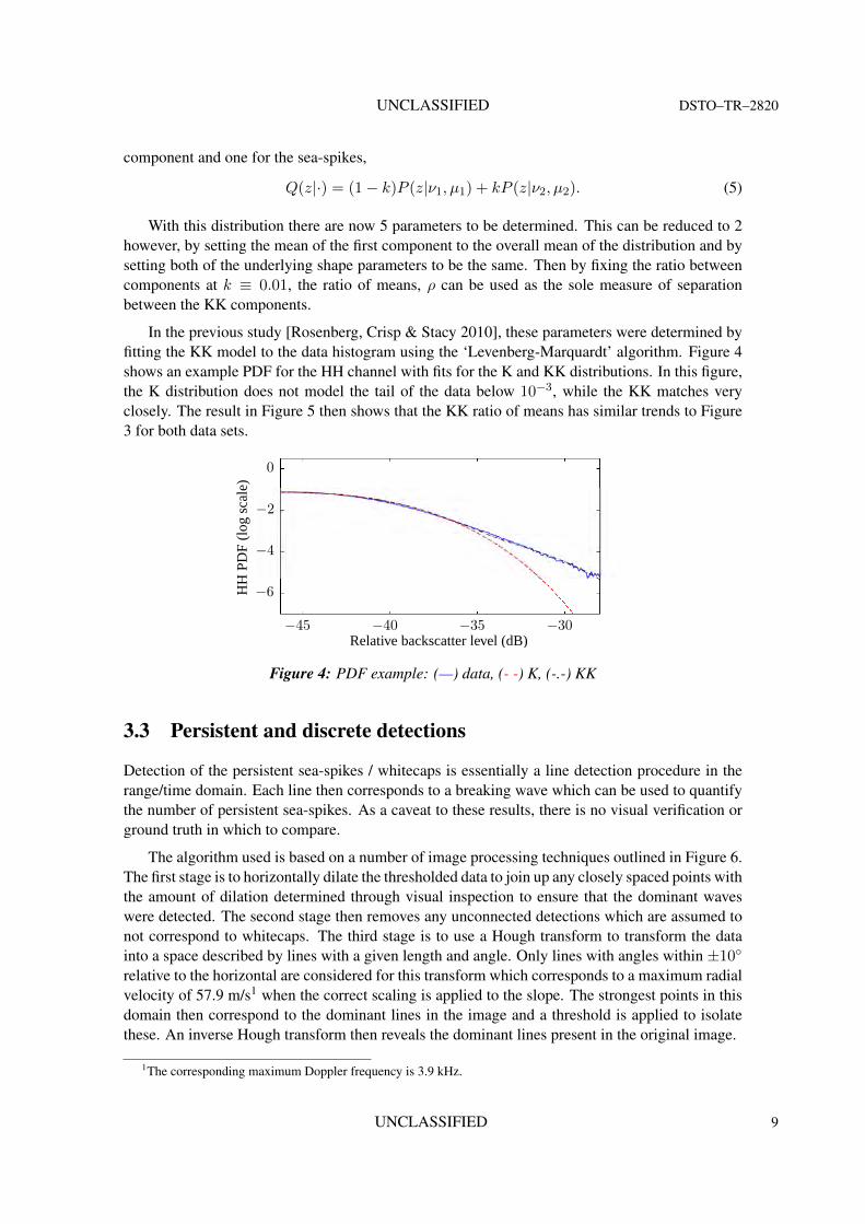
In the previous study [Rosenberg, Crisp & Stacy 2010], these parameters were determined byfitting the KK model to the data histogram using the ‘Levenberg-Marquardt’ algorithm. Figure 4shows an example PDF for the HH channel with fits for the K and KK distributions. In this figure,the K distribution does not model the tail of the data below 10−3, while the KK matches veryclosely. The result in Figure 5 then shows that the KK ratio of means has similar trends to Figure3 for both data sets.

HH

PDF

(log

scal

e)

Relative backscatter level (dB)−45 −40 −35 −30

−6

−4

−2

0

Figure 4: PDF example: (—) data, (- -) K, (-.-) KK

3.3 Persistent and discrete detections

Detection of the persistent sea-spikes / whitecaps is essentially a line detection procedure in therange/time domain. Each line then corresponds to a breaking wave which can be used to quantifythe number of persistent sea-spikes. As a caveat to these results, there is no visual verification orground truth in which to compare.

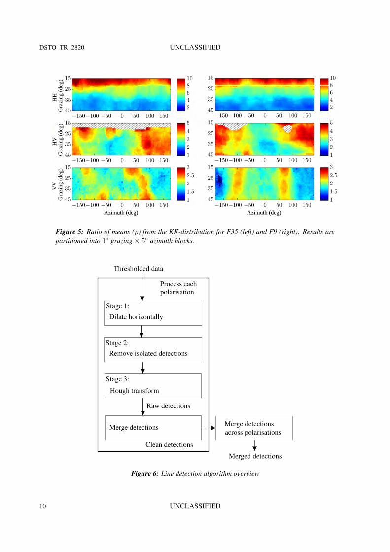
The algorithm used is based on a number of image processing techniques outlined in Figure 6.The first stage is to horizontally dilate the thresholded data to join up any closely spaced points withthe amount of dilation determined through visual inspection to ensure that the dominant waveswere detected. The second stage then removes any unconnected detections which are assumed tonot correspond to whitecaps. The third stage is to use a Hough transform to transform the datainto a space described by lines with a given length and angle. Only lines with angles within ±10◦

relative to the horizontal are considered for this transform which corresponds to a maximum radialvelocity of 57.9 m/s1 when the correct scaling is applied to the slope. The strongest points in thisdomain then correspond to the dominant lines in the image and a threshold is applied to isolatethese. An inverse Hough transform then reveals the dominant lines present in the original image.

1The corresponding maximum Doppler frequency is 3.9 kHz.

UNCLASSIFIED 9


Azimuth (deg)

VV

Gra

zing

(deg

)H

VG

razi

ng

(deg

)H

HG

razi

ng

(deg

)

−150−100 −50 0 50 100 150

−150−100 −50 0 50 100 150

−150−100 −50 0 50 100 150

1

1.5

2

2.5

315

25

35

45

1

2

3

4

515

25

35

45

2

4

6

8

1015

25

35

45

Azimuth (deg)

−150−100 −50 0 50 100 150

−150−100 −50 0 50 100 150

−150−100 −50 0 50 100 150

1

1.5

2

2.5

315

25

35

45

1

2

3

4

515

25

35

45

2

4

6

8

1015

25

35

45

Figure 5: Ratio of means (ρ) from the KK-distribution for F35 (left) and F9 (right). Results arepartitioned into 1◦ grazing × 5◦ azimuth blocks.

Thresholded data

Dilate horizontally

Remove isolated detections

Hough transform

Merge detections

Raw detections

Merge detections

Process each

Merged detections

Clean detections

across polarisations

polarisation

Stage 1:

Stage 2:

Stage 3:

Figure 6: Line detection algorithm overview

10 UNCLASSIFIED


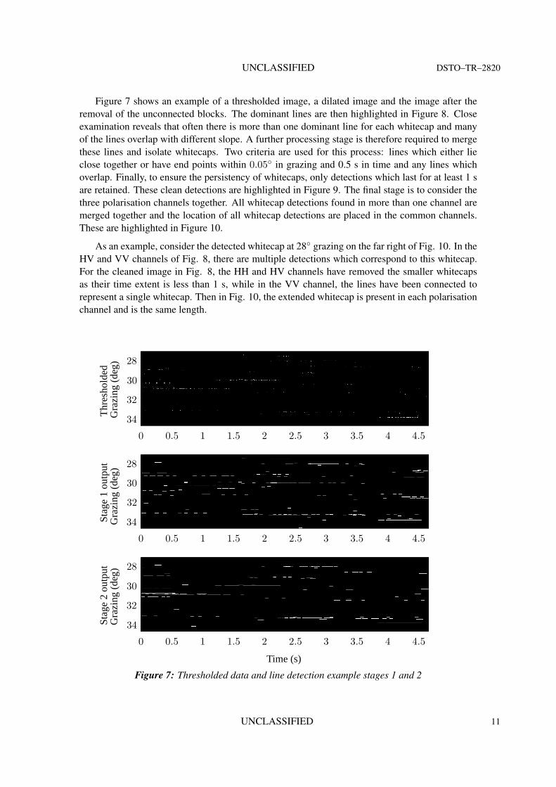
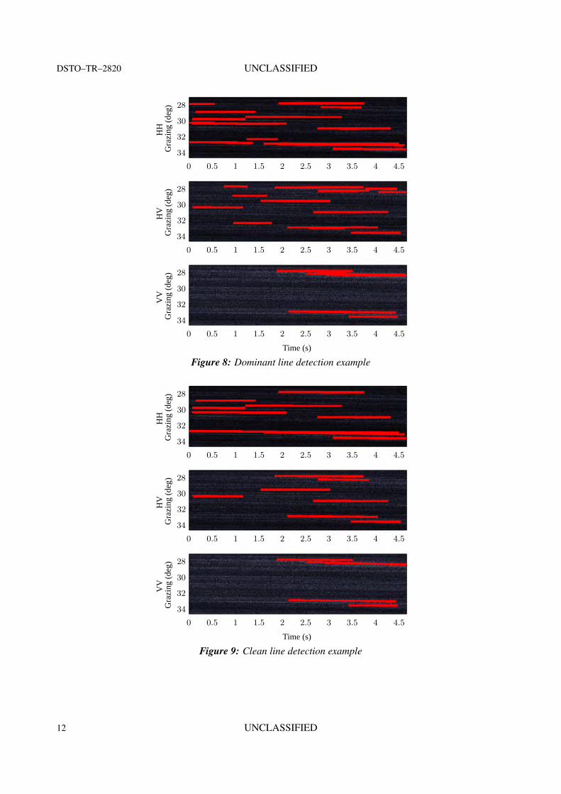
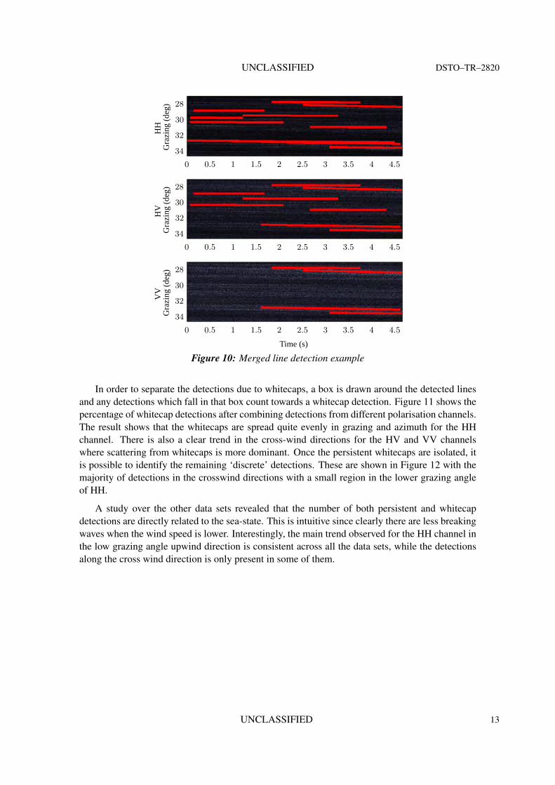
Figure 7 shows an example of a thresholded image, a dilated image and the image after theremoval of the unconnected blocks. The dominant lines are then highlighted in Figure 8. Closeexamination reveals that often there is more than one dominant line for each whitecap and manyof the lines overlap with different slope. A further processing stage is therefore required to mergethese lines and isolate whitecaps. Two criteria are used for this process: lines which either lieclose together or have end points within 0.05◦ in grazing and 0.5 s in time and any lines whichoverlap. Finally, to ensure the persistency of whitecaps, only detections which last for at least 1 sare retained. These clean detections are highlighted in Figure 9. The final stage is to consider thethree polarisation channels together. All whitecap detections found in more than one channel aremerged together and the location of all whitecap detections are placed in the common channels.These are highlighted in Figure 10.

As an example, consider the detected whitecap at 28◦ grazing on the far right of Fig. 10. In theHV and VV channels of Fig. 8, there are multiple detections which correspond to this whitecap.For the cleaned image in Fig. 8, the HH and HV channels have removed the smaller whitecapsas their time extent is less than 1 s, while in the VV channel, the lines have been connected torepresent a single whitecap. Then in Fig. 10, the extended whitecap is present in each polarisationchannel and is the same length.

Time (s)

Stag

e2

outp

utG

razi

ng(d

eg)

Stag

e1

outp

utG

razi

ng(d

eg)

Thr

esho

lded

Gra

zing

(deg

)

0 0.5 1 1.5 2 2.5 3 3.5 4 4.5

0 0.5 1 1.5 2 2.5 3 3.5 4 4.5

0 0.5 1 1.5 2 2.5 3 3.5 4 4.5

28

30

32

34

28

30

32

34

28

30

32

34

Figure 7: Thresholded data and line detection example stages 1 and 2

UNCLASSIFIED 11


VV

Gra

zing

(deg

)

Time (s)

HV

Gra

zing

(deg

)H

HG

razi

ng(d

eg)

0 0.5 1 1.5 2 2.5 3 3.5 4 4.5

0 0.5 1 1.5 2 2.5 3 3.5 4 4.5

0 0.5 1 1.5 2 2.5 3 3.5 4 4.5

28

30

32

34

28

30

32

34

28

30

32

34

Figure 8: Dominant line detection example

VV

Gra

zing

(deg

)

Time (s)

HV

Gra

zing

(deg

)H

HG

razi

ng(d

eg)

0 0.5 1 1.5 2 2.5 3 3.5 4 4.5

0 0.5 1 1.5 2 2.5 3 3.5 4 4.5

0 0.5 1 1.5 2 2.5 3 3.5 4 4.5

28

30

32

34

28

30

32

34

28

30

32

34

Figure 9: Clean line detection example

12 UNCLASSIFIED


VV

Gra

zing

(deg

)

Time (s)

HV

Gra

zing

(deg

)H

HG

razi

ng(d

eg)

0 0.5 1 1.5 2 2.5 3 3.5 4 4.5

0 0.5 1 1.5 2 2.5 3 3.5 4 4.5

0 0.5 1 1.5 2 2.5 3 3.5 4 4.5

28

30

32

34

28

30

32

34

28

30

32

34

Figure 10: Merged line detection example

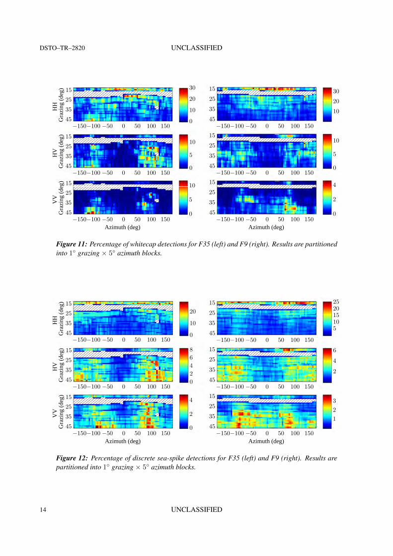
In order to separate the detections due to whitecaps, a box is drawn around the detected linesand any detections which fall in that box count towards a whitecap detection. Figure 11 shows thepercentage of whitecap detections after combining detections from different polarisation channels.The result shows that the whitecaps are spread quite evenly in grazing and azimuth for the HHchannel. There is also a clear trend in the cross-wind directions for the HV and VV channelswhere scattering from whitecaps is more dominant. Once the persistent whitecaps are isolated, itis possible to identify the remaining ‘discrete’ detections. These are shown in Figure 12 with themajority of detections in the crosswind directions with a small region in the lower grazing angleof HH.

A study over the other data sets revealed that the number of both persistent and whitecapdetections are directly related to the sea-state. This is intuitive since clearly there are less breakingwaves when the wind speed is lower. Interestingly, the main trend observed for the HH channel inthe low grazing angle upwind direction is consistent across all the data sets, while the detectionsalong the cross wind direction is only present in some of them.

UNCLASSIFIED 13


VV

Gra

zing

(deg

)

Azimuth (deg)

HV

Gra

zing

(deg

)H

HG

razi

ng(d

eg)

−150−100 −50 0 50 100 150

−150−100 −50 0 50 100 150

−150−100 −50 0 50 100 150

0

5

1015

25

35

45

0

5

10

15

25

35

45

0

10

20

3015

25

35

45

Azimuth (deg)−150−100 −50 0 50 100 150

−150−100 −50 0 50 100 150

−150−100 −50 0 50 100 150

0

2

415

25

35

45

0

5

1015

25

35

45

10

20

3015

25

35

45

Figure 11: Percentage of whitecap detections for F35 (left) and F9 (right). Results are partitionedinto 1◦ grazing × 5◦ azimuth blocks.

VV

Gra

zing

(deg

)

Azimuth (deg)

HV

Gra

zing

(deg

)H

HG

razi

ng(d

eg)

−150−100 −50 0 50 100 150

−150−100 −50 0 50 100 150

−150−100 −50 0 50 100 150

0

2

415

25

35

45

0

2

4

6

815

25

35

45

0

10

20

15

25

35

45

Azimuth (deg)−150−100 −50 0 50 100 150

−150−100 −50 0 50 100 150

−150−100 −50 0 50 100 150

1

2

315

25

35

45

2

4

615

25

35

45

5

10

15

20

2515

25

35

45

Figure 12: Percentage of discrete sea-spike detections for F35 (left) and F9 (right). Results arepartitioned into 1◦ grazing × 5◦ azimuth blocks.

14 UNCLASSIFIED


3.4 Sea-spike characteristics

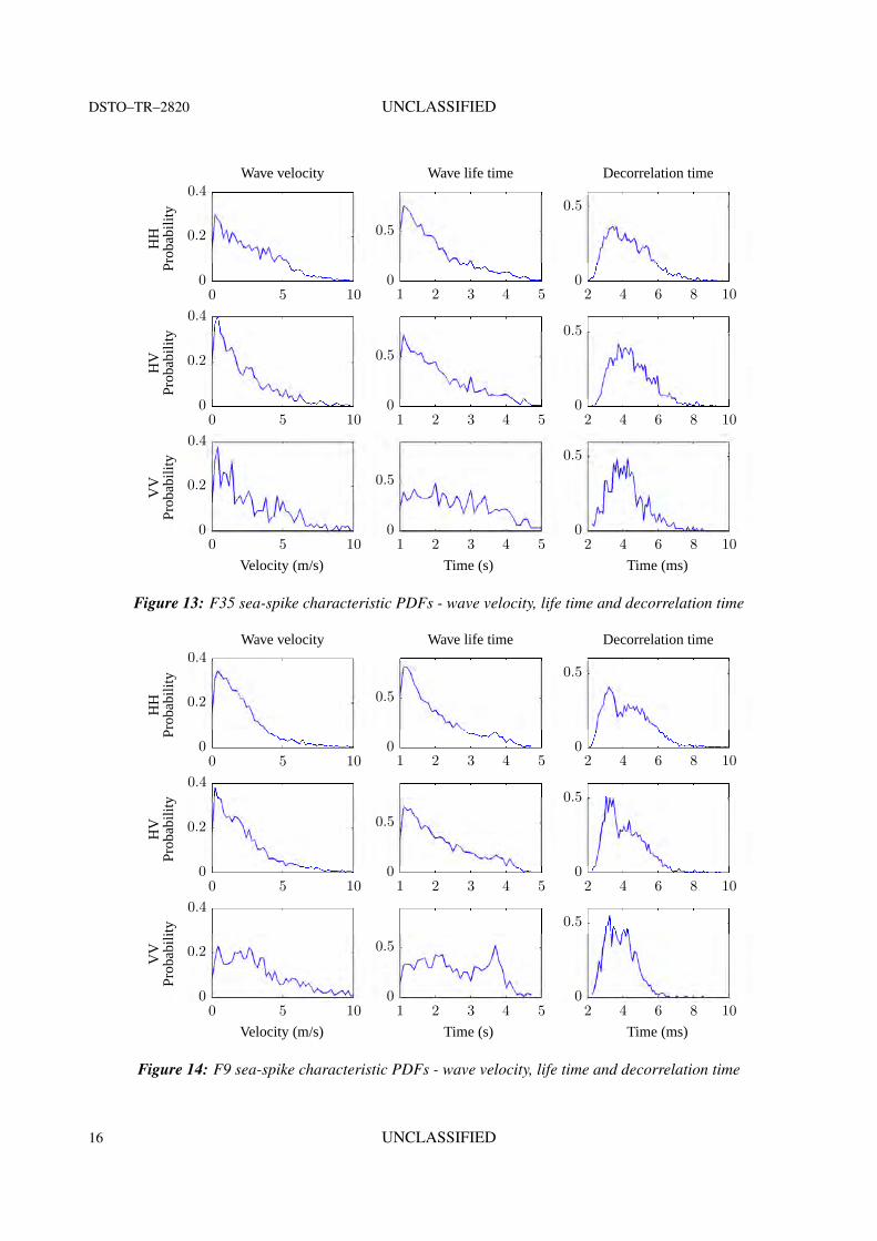
To further characterise the sea-spikes, a number of parameters have been extracted from the data.The first three are the wave velocity, life time and decorrelation time. The mean values for eachpolarisation channel are given in Tables 3-4 for the F35 and F9 data sets, with their PDFs shownin Figures 13-14.

The absolute wave velocity and life times are determined from the slope and time extent ofthe waves in the range/time domain respectively. However, the wave velocity is measured in theradial direction vr which will vary as the radar look direction / azimuth angle θaz varies. To obtainthe true wave velocity vw, this radial velocity needs to be projected along the wave direction θw,

vw = vr cos(θaz − θw). (6)

The PDFs both resemble a negative exponential distribution with little change over polarisation.The mean values are between 2-3 m/s which is significantly less than the measured wind speed forthese two days.

The wave life time varies from 1 to 5 s with a negative exponential decay observed for the HHand HV channels with a mean of approximately 2 s. For the VV channel, there is a more uniformspread. The autocorrelation function (ACF) is related to the mean Doppler spectrum through aFourier transform and will in general be complex. The temporal decorrelation is measured at thepoint where the absolute value of the ACF decays to 1/e. This parameter is important as it iscommonly used to quantify the level of temporal correlation present in the observed sea-clutter.The mean values vary between 3.9 to 4.5 ms with little difference between polarisations. Note thatthese values do not account for the broadening of the Doppler spectrum due to the moving radarplatform and hence the true wave decorrelation times will be slightly longer. This is not expectedto be significant however as the spikes are only present in a small region of the beam.

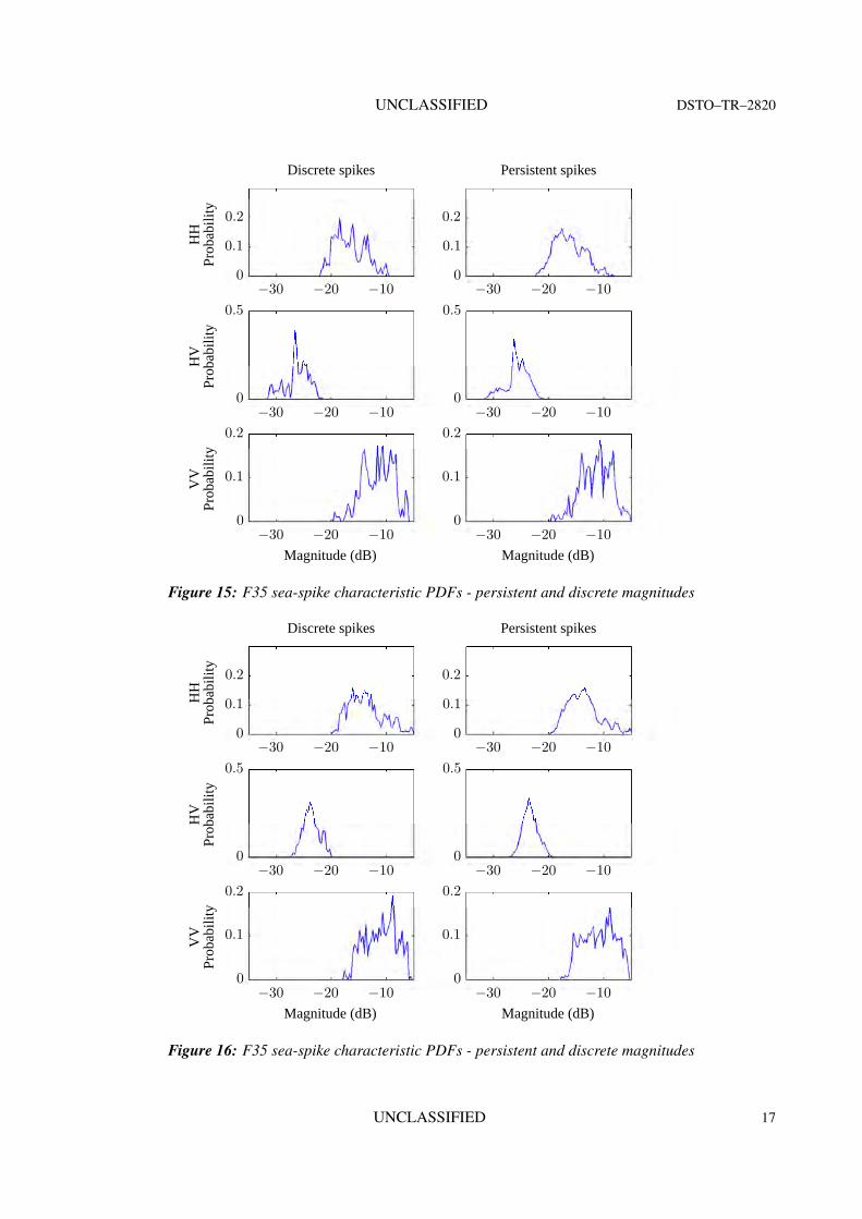
The next results in Figures 15-16 show the PDFs for the discrete and persistent scatterers.The mean values reveal that there is little difference between the magnitudes of the two scatteringtypes. The VV channel has the largest value, followed by HH and then HV. Between the two datasets, the mean levels vary up to 3 dB for the HH channel, while the VV channel differs by 0.6 dB.

Table 3: F35 sea-spike characteristic means

HH HV VVVelocity (m/s) 2.80 2.29 2.96Life time (s) 2.02 2.12 2.53Decorrelation time (ms) 4.49 4.49 4.25Discrete magnitude (dB) -15.73 -25.76 -10.77Persistent magnitude (dB) -15.43 -25.31 -10.60

Table 4: F9 sea-spike characteristic means

HH HV VVVelocity (m/s) 2.14 2.26 3.37Life time (s) 1.98 2.14 2.54Decorrelation time (ms) 4.31 4.12 3.87Discrete magnitude (dB) -12.57 -23.40 -10.18Persistent magnitude (dB) -12.54 -23.13 -9.97

UNCLASSIFIED 15


Time (ms)Time (s)

VV

Prob

abili

ty

Velocity (m/s)

HV

Prob

abili

tyDecorrelation timeWave life timeWave velocity

HH

Prob

abili

ty

2 4 6 8 101 2 3 4 50 5 10

2 4 6 8 101 2 3 4 50 5 10

2 4 6 8 101 2 3 4 50 5 10

0

0.5

0

0.5

0

0.2

0.4

0

0.5

0

0.5

0

0.2

0.4

0

0.5

0

0.5

0

0.2

0.4

Figure 13: F35 sea-spike characteristic PDFs - wave velocity, life time and decorrelation time

Time (ms)Time (s)

VV

Prob

abili

ty

Velocity (m/s)

HV

Prob

abili

ty

Decorrelation timeWave life timeWave velocity

HH

Prob

abili

ty

2 4 6 8 101 2 3 4 50 5 10

2 4 6 8 101 2 3 4 50 5 10

2 4 6 8 101 2 3 4 50 5 10

0

0.5

0

0.5

0

0.2

0.4

0

0.5

0

0.5

0

0.2

0.4

0

0.5

0

0.5

0

0.2

0.4

Figure 14: F9 sea-spike characteristic PDFs - wave velocity, life time and decorrelation time

16 UNCLASSIFIED


Magnitude (dB)Magnitude (dB)

VV

Prob

abili

tyH

VPr

obab

ility

Persistent spikesDiscrete spikes

HH

Prob

abili

ty

−30 −20 −10−30 −20 −10

−30 −20 −10−30 −20 −10

−30 −20 −10−30 −20 −10

0

0.1

0.2

0

0.1

0.2

0

0.5

0

0.5

0

0.1

0.2

0

0.1

0.2

Figure 15: F35 sea-spike characteristic PDFs - persistent and discrete magnitudes

Magnitude (dB)Magnitude (dB)

VV

Prob

abili

tyH

VPr

obab

ility

Persistent spikesDiscrete spikes

HH

Prob

abili

ty

−30 −20 −10−30 −20 −10

−30 −20 −10−30 −20 −10

−30 −20 −10−30 −20 −10

0

0.1

0.2

0

0.1

0.2

0

0.5

0

0.5

0

0.1

0.2

0

0.1

0.2

Figure 16: F35 sea-spike characteristic PDFs - persistent and discrete magnitudes

UNCLASSIFIED 17


3.5 Doppler spectrum

A dual-pol run from the F9 dataset is now used to demonstrate the relationship between persistentsea-spikes and the Doppler spectrum. The data is collected over two consecutive runs and it istherefore assumed that the combined mean Doppler spectrum is representative of an equivalentfull-pol system with a higher PRF of 600 Hz. To form the final Doppler spectrum, it must firstbe unwrapped using an estimate of the Doppler centroid. However due to uncertainties in themotion compensation, the absolute Doppler origin is not known. Therefore to ensure the correctseparation between channels, the VV channel is centred at the Doppler origin and the HH and HVchannels are shifted by the difference between HH and VV and HV and VV respectively.

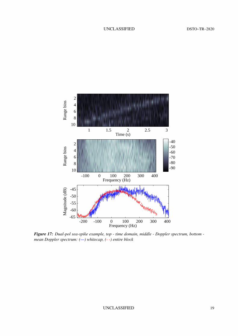
Figure 17 shows a whitecap selected from the upwind direction of the HH channel spanning 3 sin time and 10 range bins. The middle plot shows its Doppler spectrum over the 10 range bins andthe bottom plot shows the mean Doppler spectrum. To highlight the sea-spike, the mean Dopplerspectrum of the entire data block has been plotted as a comparison2. The sea-spike component canthen be seen at a higher frequency than the overall mean spectrum. Clearly, there are at least twocomponents which can be isolated and therefore modelled.

Walker’s mean Doppler spectrum model [Walker 2001a], consists of three types of scatteringreferred to as ‘Bragg’, ‘whitecap’ and discrete ‘sea-spike events’. He models each of these scat-tering types with Gaussian lineshapes with the overall spectrum for each polarisation consistingof a linear combination of these components. The Bragg scattering component is formed by smallripples on top of the longer ocean waves, causing the VV polarisation to have a greater amplitudethan HH, while the whitecap component is associated with the rough whitecaps formed at sea andhave a weaker polarisation dependence. Walker reports that at low grazing angles this componentis noticeably stronger than the Bragg scattering, particularly in HH. Sea-spikes are associated withthe crest of waves and are virtually non-existent in the VV spectrum. They last for a much shorterperiod of time than the other returns and are coherent over that time.

Referring to Figure 11 which relates to the persistent scatterers or whitecaps, there are manycommon peaks in both the HH and VV channels, with a lot of detections present in HH but notin VV. This result shows that there are common components in both channels. However, there arealso many extra whitecaps detected in the HH channel. Figure 12 also demonstrates that there aremany discrete scatterers in the VV channel. As a result, the two assumptions that the whitecapcomponent is identical in both HH and VV and that discrete scatterers from the VV channel arenegligent are not correct. Hence Walker’s mean Doppler spectrum model is not accurate at thesegrazing angles.

2Note that the Doppler spectrum has been spread due to the azimuth beampattern of the moving radar platform.

18 UNCLASSIFIED


Ran

gebi

ns

Time (s)

Ran

gebi

ns

Frequency (Hz)

Mag

nitu

de(d

B)

Frequency (Hz)-200 -100 0 100 200 300 400

-100 0 100 200 300 400

1 1.5 2 2.5 3

-65

-60

-55

-50

-45

-90-80-70-60-50-402

4

6

8

10

2

4

6

8

10

Figure 17: Dual-pol sea-spike example, top - time domain, middle - Doppler spectrum, bottom -mean Doppler spectrum: (—) whitecap, (- -) entire block

UNCLASSIFIED 19


4 Conclusion

This report has investigated the detection and characterisation of sea-spikes with the goal of beingable to better distinguish them from targets of interest. The approach used was to threshold themagnitude of the raw backscatter data in the range/time domain. The first result looked at thepercentage of sea-spikes present in the Ingara high grazing angle sea-clutter data. The resultsshowed that the majority occur in the lower grazing angle region for the HH channel and wereslightly higher in the cross wind directions for the other two polarisation channels. These resultswere then verified by comparing the trends with a separate analysis which used the KK PDF tomodel the sea-clutter.

An image processing algorithm was then used to isolate the discrete and persistent scatterersand test whether Walker’s mean Doppler spectrum model was valid with the higher grazing angles.The results found that the whitecaps were spread quite evenly in grazing and azimuth for the HHchannel with a clear trend in the cross-wind directions for the HV and VV channels. While therewere many common peaks in both the HH and VV channels, there were however, a lot of detectionspresent in HH but not in VV. There were also many discrete scatterers detected in the VV channel.This indicates that Walker’s three channel model is not totally valid at high grazing angles. Futurework will look at a modified model to represent the mean Doppler spectrum at high grazing anglesand how these new results can be used to improve target detection in the maritime environment.

20 UNCLASSIFIED


References

Blacknell, D. & Tough, R. J. A. (2001) Parameter estimation for the K-distribution based on [zlog(z)], IEE Proceedings of Radar, Sonar and Navigation 148(6), 309–312.

Crisp, D. J., Kyprianou, R., Rosenberg, L. & Stacy, N. J. (2008) Modelling X-band sea clutter atmoderate grazing angles, in IEEE International Radar Conference, pp. 596–601.

Crisp, D. J., Stacy, N. J. & Goh, A. S. (2006) Ingara Medium-High Incidence Angle PolarimetricSea Clutter Measurements and Analysis, Technical Report DSTO-TR-1818, DSTO.

Departent of Defence, Australia (2012) Air 7000 project description.http://www.defence.gov.au/capability/AIR7000/.

Dong, Y. (2006) Distribution of X-Band High Resolution and High Grazing Angle Sea Clutter,Research Report DSTO-RR-0316, DSTO.

Dong, Y. & Crisp, D. J. (2008) The Euler decomposition and its application to sea clutter analysis,in IEEE International radar conference.

Duncan, J. R., Keller, W. C. & Wright, J. W. (1974) Fetch and wind speed dependence of dopplerspectra, Radio Science 9, 809–819.

Greco, M., Stinco, P. & Gini, F. (2010) Identification and analysis of sea radar clutter spikes, IETJournal of Radar, Sonar and Navigation 4(2), 239–250.

Jessup, A. T., Keller, W. C. & Melville, W. K. (1990) Measurement of sea spikes in microwavebackscatter at moderate incidence, Journal of Geophysical Research 95(C6), 9679–9688.

Jessup, A. T., Melville, W. K. & Keller, W. C. (1991) Breaking waves affecting microwavebackscatter, 1. detection and verification, Journal of Geophysical Research 96(C11), 20,547–20,559.

Keller, M. R., Gotwols, B. L. & Chapman, R. D. (2002) Multiple sea spike definitions: reducingthe clutter, in IEEE International Geoscience and Remote Sensing Symposium, pp. 940–942.

Lee, P. H. Y., Barter, J. D., Beach, K. L., Hindman, C. L., Lake, B. M., Rungaldier, H., Shelton,J. C., Williams, A. B., Yee, R. & Yuen, H. C. (1995a) X-band microwave backscattering fromocean waves, Journal of Geophysical Research 100(C2), 2591–2611.

Lee, P. H. Y., Barter, J. D., Caponi, E., Hidman, C. L., Lake, B. M., Rungaldier, H. & Shelton, J. C.(1995b) Power spectral lineshapes of microwave radiation backscattered from sea surfaces atsmall grazing angles, IEE Proceedings of Radar, Sonar and Navigation 142(5), 252–258.

Liu, L. & Frasier, S. J. (1998) Measurement and classification of low-grazing-angle radar seaspikes, IEEE Transactions on Antennas and Propagation 46(1), 27–40.

Long, M. W. (2001) Radar Reflectivity of Land and Sea - Third Edition, Artech House.

Melief, H. W., Greidanus, H., van Genderen, P. & Hoogeboom, P. (2006) Analysis of sea spikes inradar sea clutter data, IEEE Transactions on Geoscience and Remote Sensing 44(4), 985–993.

UNCLASSIFIED 21


Nathanson, F. E., Reilly, J. P. & Cohen, M. N. (1991) Radar Design Principles - Second Edition,McGraw-Hill.

Parfitt, A. & Nikolic, N. (2001) A dual-polarised wideband planar array for X-band syntheticaperture radar, in IEEE Antennas and Propagation Society International Symposium, Vol. 2,pp. 464–467.

Peake, W. H. (1959) Theory of radar return from terrain, in IRE Convention Record, pp. 27–41.

Quegan, S. (1994) Unified algorithm for phase and cross-talk calibration of polarimetric data:Theory and observations, IEEE Transactions on Geoscience and Remote Sensing 32(1), 89–99.

Rosenberg, L., Crisp, D. J. & Stacy, N. J. (2008) Characterisation of low-PRF X-band sea-clutterDoppler spectra, in IEEE International Radar Conference, pp. 100–105.

Rosenberg, L., Crisp, D. J. & Stacy, N. J. (2010) Analysis of the KK-distribution with mediumgrazing angle sea-clutter, IET Proceedings of Radar Sonar and Navigation 4(2), 209–222.

Rosenberg, L. & Stacy, N. J. (2008) Analysis of medium angle X-band sea-clutter Doppler spectra,in IEEE Radarcon Conference.

Skolnik, M. I. (1990) Radar Handbook, 2 edn, McGraw-Hill.

Stacy, N. J. S., Badger, D. P., Goh, A. S., Preiss, M. & Williams, M. L. (2003) The DSTO Ingaraairbone X-band SAR polarimetric upgrade: first results, in IEEE International Geoscienceand Remote Sensing Symposium, Vol. 7, pp. 4474 – 4476.

Valenzuela, G. R. & Laing, M. B. (1970) Study of Doppler spectra of radar sea echo, Journal ofGeophysical Research 75, 551–563.

Walker, D. (2001a) Doppler modelling of radar sea clutter, IEE Proceedings of Radar, Sonar andNavigation 148(2), 73–80.

Walker, D. (2001b) Model and Characterisation of Radar Sea Clutter, PhD thesis, UniversityCollege London.

Ward, K. D., Tough, R. J. A. & Watts, S. (2006) Sea Clutter: Scattering, the K-Distribution andRadar Performance, The Institute of Engineering Technology.

Werle, B. O. (1995) Sea backscatter, spikes and wave group observations at low grazing angles, inIEEE International Radar Conference, pp. 187–195.

Wright, J. W. (1968) A new model for sea clutter, IEEE Transactions on Antennas and Propagation16(2), 217–223.

22 UNCLASSIFIED

Page classification: UNCLASSIFIED

DEFENCE SCIENCE AND TECHNOLOGY ORGANISATIONDOCUMENT CONTROL DATA

1. CAVEAT/PRIVACY MARKING

2. TITLE

Sea-Spike Detection in High Grazing Angle X-bandSea-Clutter

3. SECURITY CLASSIFICATION

Document (U)Title (U)Abstract (U)

4. AUTHOR

Luke Rosenberg

5. CORPORATE AUTHOR

Defence Science and Technology OrganisationPO Box 1500Edinburgh, South Australia 5111, Australia

6a. DSTO NUMBER

DSTO–TR–28206b. AR NUMBER

015-5716c. TYPE OF REPORT

Technical Report7. DOCUMENT DATE

April 20128. FILE NUMBER

2012/1144904/19. TASK NUMBER

AIR700010. TASK SPONSOR

DGAD11. No. OF PAGES

2212. No. OF REFS

3113. URL OF ELECTRONIC VERSION

http://www.dsto.defence.gov.au/publications/scientific.php

14. RELEASE AUTHORITY

Chief, Electronic Warfare and Radar Division

15. SECONDARY RELEASE STATEMENT OF THIS DOCUMENT

Approved for Public ReleaseOVERSEAS ENQUIRIES OUTSIDE STATED LIMITATIONS SHOULD BE REFERRED THROUGH DOCUMENT EXCHANGE, PO BOX 1500, EDINBURGH, SOUTH AUSTRALIA 5111

16. DELIBERATE ANNOUNCEMENT

No Limitations17. CITATION IN OTHER DOCUMENTS

No Limitations18. DSTO RESEARCH LIBRARY THESAURUS

Sea-clutter, sea-spike detection, radar19. ABSTRACT

Knowledge of radar sea-clutter phenomenology allows accurate models to be developed for assessing targetdetection performance. The majority of work in this area has been at low-grazing angles from clifftops orwave tanks and does not consider scattering in the high grazing angle region beyond 10◦. To improve ourunderstanding at high grazing angles 15◦ to 45◦, the DSTO’s Ingara airborne X-band fully polarimetric radar hasbeen used to collect 12 days worth of sea-clutter data. This report focuses on understanding the characteristics ofsea-spikes as they are often the cause of false detections in a radar processor. Using the Ingara data, a thresholdis used to isolate these scatterers in the range/time domain with results verified against the KK probabilitydistribution function. Detections due to discrete and persistent scattering are then isolated to provide moreinformation regarding the underlying cause of sea-spikes and answer the question of whether Walker’s threecomponent mean Doppler spectrum model is suitable at high grazing angles.

Page classification: UNCLASSIFIED

Documents

Sea-spike Detection in High Grazing Angle X-band Sea-Clutter · UNCLASSIFIED Sea-Spike Detection in High Grazing Angle X-band Sea-Clutter Luke Rosenberg Electronic Warfare and Radar