Journal of

Marine Science and Engineering

Article

Sea Waves Transport of Inertial Micro-Plastics:Mathematical Model and Applications

Alessandro Stocchino * , Francesco De Leo and Giovanni Besio

Department of Civil, Chemical and Environmental Engineering, University of Genoa, Via Montallegro 1,16145 Genoa, Italy; francesco.deleo@edu.unige.it (F.D.L.); giovanni.besio@unige.it (G.B.)* Correspondence: alessandro.stocchino@unige.it; Tel.: +39-010-33-56576

Received: 7 November 2019; Accepted: 12 December 2019; Published: 17 December 2019 �����������������

Abstract: Plastic pollution in seas and oceans has recently been recognized as one of the mostimpacting threats for the environment, and the increasing number of scientific studies proves thatthis is an issue of primary concern. Being able to predict plastic paths and concentrations withinthe sea is therefore fundamental to properly face this challenge. In the present work, we evaluatedthe effects of sea waves on inertial micro-plastics dynamics. We hypothesized a stationary inputnumber of particles in a given control volume below the sea surface, solving their trajectories anddistributions under a second-order regular wave. We developed an exhaustive group of datasets,spanning the most plausible values for particles densities and diameters and wave characteristics,with a specific focus on the Mediterranean Sea. Results show how the particles inertia significantlyaffects the total transport of such debris by waves.

Keywords: micro-plastics; particle inertia; stokes wave; stokes drift; Mediterranean Sea

1. Introduction

In the last decades the production and consumption of plastic products has drastically increased.Most of our daily activities and behaviors involve the use of plastic, e.g., when packaging food andgoods or wearing synthetic clothes, as a couple of instances among many others. It is estimated that weglobally use in excess of 260 million tonnes of plastic per year, accounting for approximately 8 per centof world oil production [1]. The proper disposal of plastic waste has consequently become a centralissue of our times, still far from being completely overcome [2]. The lack of regulations and practicesable to allow a sustainable and efficient waste management has often led to undesirable releases ofplastic within the marine environment [3], resulting in a substantial volume of debris added to theocean over the past 60 years [4–6]. Efficient policies should be aimed at reducing plastic consumptionand using biodegradable materials when reliable alternatives are available, and the most recent EUdirectives are indeed developing in this framework.

At first sight, to face the maritime plastic pollution requires anyway a holistic comprehensionof the plastic particles dynamic in seas and oceans. The need to tackle the plastic pollution threatwith the utmost urgency is consequently reflecting in the attention given by the scientific community,as proved by the increasing amount of papers on such topic (a partial summary can be found inHidalgo-Ruz et al. [7]). So far the transport of plastic particles was numerically simulated mainlyassuming that, in a Lagrangian sense, the single particle is non-inertial, or, in other words, it hasthe same mass-density of the carrier fluid in this case the sea water [8]. Then, the fate of a single ora cluster of neutrally buoyant particles is obtained by simply solving the trajectory equation, where theparticle position depends at any time on the Eulerian velocity field obtained by hydrodynamic modelsand/or observational data (see as an instance [9,10]). Several dynamical effects can be taken intoaccount by a specific choice of the Eulerian velocity field, which can be though in fact as a sum

J. Mar. Sci. Eng. 2019, 7, 467; doi:10.3390/jmse7120467 www.mdpi.com/journal/jmse

J. Mar. Sci. Eng. 2019, 7, 467 2 of 19

of different contributions, e.g., oceanic currents, Stokes drift, Ekman drift, and a turbulent velocitycomponent (cfr. [11–18] among others). Assuming a perfect match between sea water and plasticdebris density inhibits any physical mechanism of sedimentation, which is indeed neglected whenassuming neutrally buoyant particles. On the contrary, other approaches allowed to consider a settlingvelocity disregarding any drag-induced effect, both in a lagrangian [14,19] and in an eulerian [20]approach; the settling velocity of the particles was also taken into account in Liubartseva et al. [17],who simulated the sedimentation of particles through a statistical approach based on Montecarlosimulations. Nevertheless, it has to be pointed out that the drag may be reasonably neglected only forsome regimes of the controlling parameters, i.e., Froude and Stokes number.

However, it is well known from several field measurements that micro plastic particles can attaindifferent values of density, usually ranging from 0.85 g cm−3 to 1.41 g cm−3 for polypropylene or PPand polytetrafluoroethylene or PVC respectively, see [16,20], and the differential density of the plasticdebris can play an important role in the transport dynamics, especially for dimensions proper of themicro-plastic class. Furthermore, in sea waters the density of plastic particles can be dramaticallymodified due to biological effects, so that even particle lighter than sea water may start to settle andrise with specific periods [21,22]. In view of the above, we used a model that allows to computethe trajectory of micro-plastic particles by taking into account both the buoyancy of the particle andthe drag of the flow. We referred to micro-plastics, e.g., particles characterized by diameters smallerthan 5 mm, according to the definition of Arthur et al. [23]. These pieces of debris are of particularconcern as they are difficult to intercept and, moreover, they are easily ingested by most of the marinespecies [24,25].

The paper is structured as follows: in Section 2 the numerical model employed and the testingsets are introduced. Then, in Section 3 results are shown and further discussed and summarizedin Section 4.

2. Methods

The model proposed allows to assess time-dependent plastic accumulation along the z verticaldirection in the 2D x-z plain, under second-order regular linear waves, referring to a prescribed particlevolumetric concentration. To this end, we reproduced a sequence of particle releases representingan infinite availability of micro-plastics at a given location, under different initial conditions. We variedthe parameters that might affect the settling and/or the suspension of the particles, as their physicalproperties (size and density distribution) as well as the sea state features (wave heights and periods).The numerical experiments provided quantitative information regarding the path followed by plasticparticles owing to the Stokes drift, their horizontal (x component) and vertical (z component) velocitiesand, finally, on their vertical distribution.

This section formulates the conceptual model adopted in this study. It shows the wave and theparticle dynamics equations, which are solved numerically in order to obtain the trajectories of theinertial particles representing the plastic debris.

2.1. Wave Model and Plastic Particle Transport Model

The flow is described by a second order monochromatic Stokes wave. The velocity field is definedon a vertical plane (x, z); the vertical and horizontal Eulerian velocities (w and u respectively) aretherefore expressed as:

w(x, z, t) =(

gkaω

)fd1 sin(kx−ωt) +

(g(ka)2

ω

)fd2 sin 2(kx−ωt) (1)

u(x, z, t) =(

gkaω

)fc1 cos(kx−ωt) +

(g(ka)2

ω

)fc2 cos 2(kx−ωt), (2)

J. Mar. Sci. Eng. 2019, 7, 467 3 of 19

where x and z are the horizontal and the vertical coordinates of the 2D plane, a is the wave amplitude,k is the wave number and ω is the angular frequency. The functions fc1, fc2, fd1 e fd2 are hyperbolicfunctions of the water depth h and the vertical coordinate z and read:

fc1 = cosh(ks)/ cosh(kz);

fc2 = 3 cosh(2ks)/4 sinh3(kz) cosh(kh);

fd1 = sinh(ks)/ sinh(kz);

fd2 = 3 sinh(2ks)/4 sinh3(kz) cosh(kh),

having defined s as (h + z).The dispersion relation linking k and ω can be expressed as follow:

ω = kU0 + σ (3)

where U0 is the value of a possible background uniform current velocity and σ is the frequency of thewave in the moving frame of reference [26].

Following this approach, the motion of a small inertial particle is described by the following setof equations [27]:

dx(t)dt

= V(t) (4)

dV(t)dt

=u(x, t)−V(t)

τ+ (1− β)g + β

du(x, t)dt

(5)

where V(t) is the Lagrangian particle velocity at the position x(t). This set of equations describes thetrajectories of small inertial particles as response to a flow field u(x, t) and subjected to a Stokes dragand gravity g. The latter effect is taken into account through the added-mass effect represented by thedimensionless parameter β, while drag response is taken into account in the first term of the secondmember of Equation (5) through the Stokes response time τ:

β =3ρ f

ρ f + 2ρp(6)

τ =d2

P12βν

(7)

where ρ f and ρp are the fluid density and particle density respectively, dP is the particle diameterand ν is the kinematic viscosity of the fluid. Note that the well known Stokes number can be readilyevaluated as St = ωτ. As a matter of fact, the Stokes number is generally defined as the ratio betweenthe characteristic times of particles (τ) and flow. In this case, the characteristic time of the flow is setequal to ω−1, precisely. For St << 1 the particle can be regarded as a passive drifter and tends tobehave as a fluid particle, whereas for Stokes number of order 1 (O(St) ' 1), inertial effects dominateleading to a behaviour dissimilar from that of passive tracers. It is worth to point out that, in theunlikely case that the plastic particle density matches the density of the fluid, Equations (4) and (5)naturally lead to the trajectory equations used to simulate a passive tracer.

The present study resumes and extends the work of Santamaria et al. [28], where the model ofMaxey & Riley [27] was solved for a first order monochromatic wave. Similarly, DiBenedetto et al. [29]referred to the same wave model and weakly inertial particles (i.e., St << 1), investigating how theshape of the latter might affect their resulting trajectories. In this work, we consider a second ordermonochromatic wave rather than a first order one, thus the Stokes drift directly arises from the wavemodel with no need to superimpose additional effects. Moreover, we include a possible uniformcurrent (U0) and we do not pose any limitation on St nor we rely on the deep water assumption for

J. Mar. Sci. Eng. 2019, 7, 467 4 of 19

resolving the wave length λ. Finally, it is worth to mention that the model here introduces only appliesto spherical particles. Although the shape of a particle is known to affect its settling velocity, this effectwas shown to be not of primary importance [30]. Indeed, this geometrical simplification is oftenadopted in the studies of the fate of particle debris based on the trajectory equation (see [14,15,20]among others), thus the results of the present analysis will refer to it.

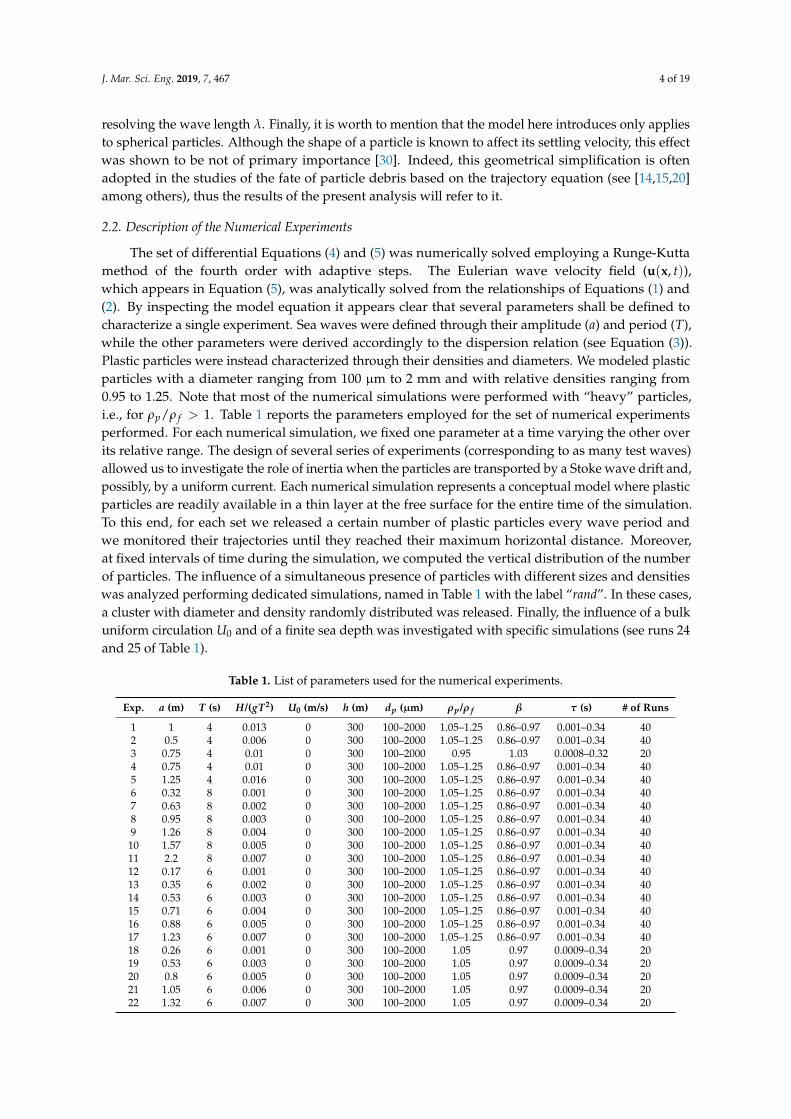
2.2. Description of the Numerical Experiments

The set of differential Equations (4) and (5) was numerically solved employing a Runge-Kuttamethod of the fourth order with adaptive steps. The Eulerian wave velocity field (u(x, t)),which appears in Equation (5), was analytically solved from the relationships of Equations (1) and(2). By inspecting the model equation it appears clear that several parameters shall be defined tocharacterize a single experiment. Sea waves were defined through their amplitude (a) and period (T),while the other parameters were derived accordingly to the dispersion relation (see Equation (3)).Plastic particles were instead characterized through their densities and diameters. We modeled plasticparticles with a diameter ranging from 100 µm to 2 mm and with relative densities ranging from0.95 to 1.25. Note that most of the numerical simulations were performed with “heavy” particles,i.e., for ρp/ρ f > 1. Table 1 reports the parameters employed for the set of numerical experimentsperformed. For each numerical simulation, we fixed one parameter at a time varying the other overits relative range. The design of several series of experiments (corresponding to as many test waves)allowed us to investigate the role of inertia when the particles are transported by a Stoke wave drift and,possibly, by a uniform current. Each numerical simulation represents a conceptual model where plasticparticles are readily available in a thin layer at the free surface for the entire time of the simulation.To this end, for each set we released a certain number of plastic particles every wave period andwe monitored their trajectories until they reached their maximum horizontal distance. Moreover,at fixed intervals of time during the simulation, we computed the vertical distribution of the numberof particles. The influence of a simultaneous presence of particles with different sizes and densitieswas analyzed performing dedicated simulations, named in Table 1 with the label “rand”. In these cases,a cluster with diameter and density randomly distributed was released. Finally, the influence of a bulkuniform circulation U0 and of a finite sea depth was investigated with specific simulations (see runs 24and 25 of Table 1).

Table 1. List of parameters used for the numerical experiments.

Exp. a (m) T (s) H/(gT2) U0 (m/s) h (m) dp (µm) ρp/ρ f β τ (s) # of Runs

1 1 4 0.013 0 300 100–2000 1.05–1.25 0.86–0.97 0.001–0.34 402 0.5 4 0.006 0 300 100–2000 1.05–1.25 0.86–0.97 0.001–0.34 403 0.75 4 0.01 0 300 100–2000 0.95 1.03 0.0008–0.32 204 0.75 4 0.01 0 300 100–2000 1.05–1.25 0.86–0.97 0.001–0.34 405 1.25 4 0.016 0 300 100–2000 1.05–1.25 0.86–0.97 0.001–0.34 406 0.32 8 0.001 0 300 100–2000 1.05–1.25 0.86–0.97 0.001–0.34 407 0.63 8 0.002 0 300 100–2000 1.05–1.25 0.86–0.97 0.001–0.34 408 0.95 8 0.003 0 300 100–2000 1.05–1.25 0.86–0.97 0.001–0.34 409 1.26 8 0.004 0 300 100–2000 1.05–1.25 0.86–0.97 0.001–0.34 4010 1.57 8 0.005 0 300 100–2000 1.05–1.25 0.86–0.97 0.001–0.34 4011 2.2 8 0.007 0 300 100–2000 1.05–1.25 0.86–0.97 0.001–0.34 4012 0.17 6 0.001 0 300 100–2000 1.05–1.25 0.86–0.97 0.001–0.34 4013 0.35 6 0.002 0 300 100–2000 1.05–1.25 0.86–0.97 0.001–0.34 4014 0.53 6 0.003 0 300 100–2000 1.05–1.25 0.86–0.97 0.001–0.34 4015 0.71 6 0.004 0 300 100–2000 1.05–1.25 0.86–0.97 0.001–0.34 4016 0.88 6 0.005 0 300 100–2000 1.05–1.25 0.86–0.97 0.001–0.34 4017 1.23 6 0.007 0 300 100–2000 1.05–1.25 0.86–0.97 0.001–0.34 4018 0.26 6 0.001 0 300 100–2000 1.05 0.97 0.0009–0.34 2019 0.53 6 0.003 0 300 100–2000 1.05 0.97 0.0009–0.34 2020 0.8 6 0.005 0 300 100–2000 1.05 0.97 0.0009–0.34 2021 1.05 6 0.006 0 300 100–2000 1.05 0.97 0.0009–0.34 2022 1.32 6 0.007 0 300 100–2000 1.05 0.97 0.0009–0.34 20

J. Mar. Sci. Eng. 2019, 7, 467 5 of 19

Table 1. Cont.

Exp. a (m) T (s) H/(gT2) U0 (m/s) h (m) dp (µm) ρp/ρ f β τ (s) # of Runs

23 1.59 6 0.009 0 300 100–2000 1.05 0.97 0.0009–0.34 2024 1.59 6 0.009 0.2 300 200–2000 1.05 0.97 0.0034–0.34 1025 1.59 6 0.009 0 20 200–2000 1.05 0.97 0.0034–0.34 10

rand1 0.5 4 0.006 0 300 100–500 0.95–1.15 0.91–1.03 0.0009–0.02 1rand2 0.75 4 0.01 0 300 100–500 0.95–1.15 0.91–1.03 0.0009–0.02 1rand3 1 4 0.013 0 300 100–500 0.95–1.15 0.91–1.03 0.0009–0.02 1rand4 1.25 4 0.016 0 300 100–500 0.95–1.15 0.91–1.03 0.0009–0.02 1

2.3. Climatology of the Sea State and Selection of Wave Parameters for the Numerical Experiments

The numerical experiments require a selection of sea state parameters (a and T) to be fed intoEquations (1) and (2). Then, the dispersion relationship (3) leads to the wave number. In order toemploy wave parameters physically meaningful, we took advantage of a long term hindcast developedat the Authors’ department (www.dicca.unige.it/meteocean, see [31–33]); the dataset covers a widetime frame of 40 years (from 1979 to 2018), and is defined all over the Mediterranean sea witha lon/lat resolution of approximately 0.1◦, providing the main wave features on a hourly base. For thepresent purpose, we analyzed time series of wave amplitude and period in several locations in theMediterranean Sea, distributed among different basins. These locations are reported in Figure 1.

6°W 1°W 4°E 9°E 14°E 19°E 24°E 29°E 34°E30°N

35°N

40°N

45°N000631

002080

004913

012841

008612

004319 004660

010955

015669

000216

002330

007276

014981

006043

011647

018902 018365020707

Figure 1. Geographical location of hindcast points used to set the wave parameters for the present study.

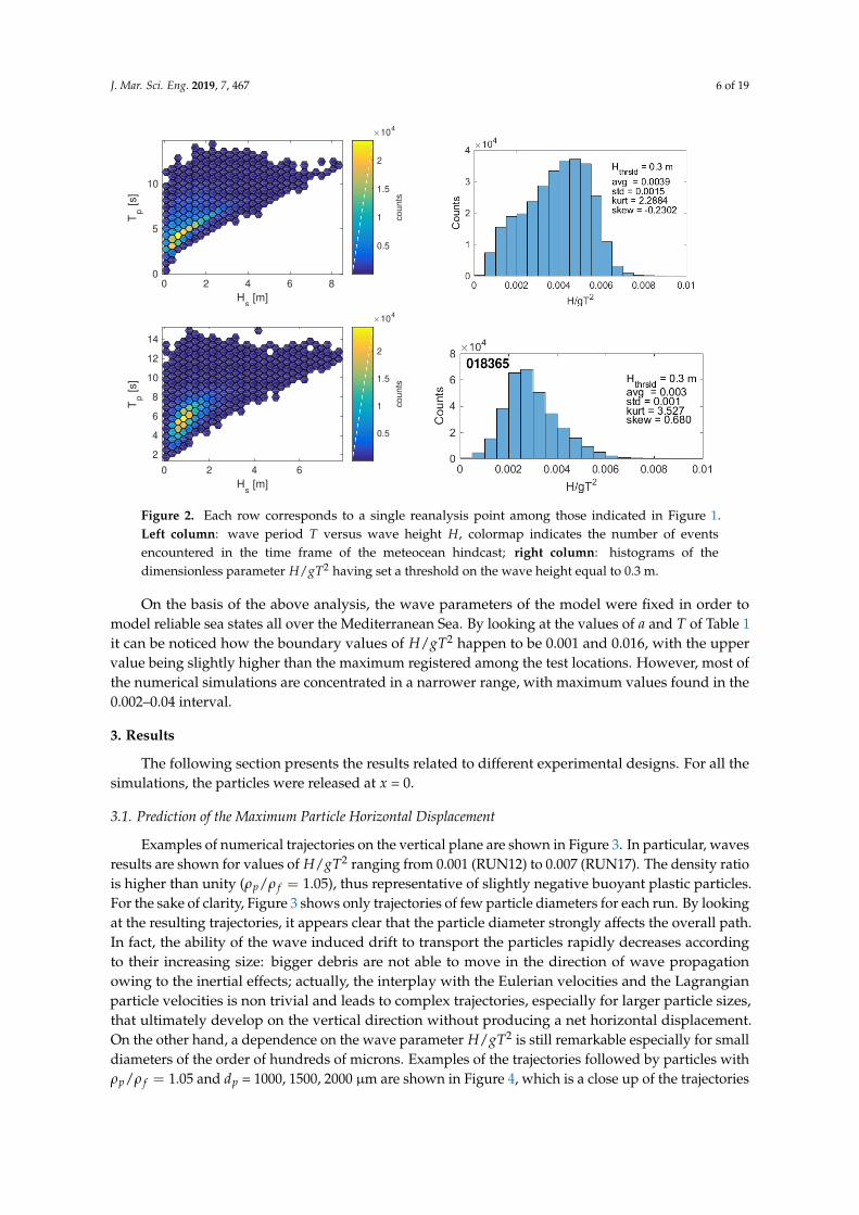
Figure 2 shows an example of the computed statistics for a couple of the selected points.We show a frequency plot of wave period against wave height H (on the left panels, havingdefined H = 2a), while the histogram plots represent the frequency of occurrence (counts) of thevalue of the dimensionless parameter H/gT2, having set a threshold for the wave height equal to0.3 m in order to get rid of the not significant sea states. The parameter H/gT2 is commonly used tosynthetically describe a sea state, since it allows to define the best performing wave model accordingto the local bottom depth [34]. In this case, the second order Stokes wave model suited well to theenvironmental condition set, thus the results of the present analysis will refer to it.

H/gT2 can be also viewed as a measure of wave steepness: for fixed values of T, increasingnumbers of H/gT2 imply higher waves; conversely, for fixed wave heights, increasing numbers ofH/gT2 imply waves with shorter periods (thus shorter wavelengths). As a general trend, locationsbelonging to the Mediterranean sea show similar features, due to the enclosed shape of the basin.This is subsequently reflecting on the frequency distributions of the parameter H/gT2, which attainssimilar values regardless the location taken into account. As Figure 2 shows, there may exist slightdifferences summarized by the values of the parameters kurtosis and skewness. In fact, Point 000631exhibits a left-skewed frequency distribution due to the higher periods characterizing the waves of thearea (most likely due to the considerable length of its fetch).

J. Mar. Sci. Eng. 2019, 7, 467 6 of 19

0 2 4 6 8

Hs [m]

0

5

10

Tp [s]

0.5

1

1.5

2

co

un

ts

×104

0 2 4 6

Hs [m]

2

4

6

8

10

12

14

Tp [s]

0.5

1

1.5

2

co

un

ts

×104

Figure 2. Each row corresponds to a single reanalysis point among those indicated in Figure 1.Left column: wave period T versus wave height H, colormap indicates the number of eventsencountered in the time frame of the meteocean hindcast; right column: histograms of thedimensionless parameter H/gT2 having set a threshold on the wave height equal to 0.3 m.

On the basis of the above analysis, the wave parameters of the model were fixed in order tomodel reliable sea states all over the Mediterranean Sea. By looking at the values of a and T of Table 1it can be noticed how the boundary values of H/gT2 happen to be 0.001 and 0.016, with the uppervalue being slightly higher than the maximum registered among the test locations. However, most ofthe numerical simulations are concentrated in a narrower range, with maximum values found in the0.002–0.04 interval.

3. Results

The following section presents the results related to different experimental designs. For all thesimulations, the particles were released at x = 0.

3.1. Prediction of the Maximum Particle Horizontal Displacement

Examples of numerical trajectories on the vertical plane are shown in Figure 3. In particular, wavesresults are shown for values of H/gT2 ranging from 0.001 (RUN12) to 0.007 (RUN17). The density ratiois higher than unity (ρp/ρ f = 1.05), thus representative of slightly negative buoyant plastic particles.For the sake of clarity, Figure 3 shows only trajectories of few particle diameters for each run. By lookingat the resulting trajectories, it appears clear that the particle diameter strongly affects the overall path.In fact, the ability of the wave induced drift to transport the particles rapidly decreases accordingto their increasing size: bigger debris are not able to move in the direction of wave propagationowing to the inertial effects; actually, the interplay with the Eulerian velocities and the Lagrangianparticle velocities is non trivial and leads to complex trajectories, especially for larger particle sizes,that ultimately develop on the vertical direction without producing a net horizontal displacement.On the other hand, a dependence on the wave parameter H/gT2 is still remarkable especially for smalldiameters of the order of hundreds of microns. Examples of the trajectories followed by particles withρp/ρ f = 1.05 and dp = 1000, 1500, 2000 µm are shown in Figure 4, which is a close up of the trajectories

J. Mar. Sci. Eng. 2019, 7, 467 7 of 19

shown in the RUN12 panel of Figure 3. Here, it can be better appreciated how the larger particles keepthe same horizontal position in which they were released.

-100

-90

-80

-70

-60

-50

-40

-30

-20

-10

0

-2 0 2 4 6 8 10 12 14

z [m

]

x [m]

RUN 12

dp=100 µmdp=200 µmdp=300 µmdp=400 µmdp=500 µm

dp=1000 µmdp=1500 µmdp=2000 µm

-100

-90

-80

-70

-60

-50

-40

-30

-20

-10

0

-10 0 10 20 30 40 50

z [m

]

x [m]

RUN 13

dp=100 µmdp=200 µmdp=300 µmdp=400 µmdp=500 µm

dp=1000 µmdp=1500 µmdp=2000 µm

-100

-90

-80

-70

-60

-50

-40

-30

-20

-10

0

-50 0 50 100 150 200 250

z [m

]

x [m]

RUN 16

dp=100 µmdp=200 µmdp=300 µmdp=400 µmdp=500 µm

dp=1000 µmdp=1500 µmdp=2000 µm

-100

-90

-80

-70

-60

-50

-40

-30

-20

-10

0

-50 0 50 100 150 200 250 300 350 400

z [m

]

x [m]

RUN 17

dp=100 µmdp=200 µmdp=300 µmdp=400 µmdp=500 µm

dp=1000 µmdp=1500 µmdp=2000 µm

Figure 3. Example of numerical trajectories for a series of simulations with increasing H/gT2 RUN 12:0.001; RUN 13: 0.002; RUN 16: 0.005; RUN 17: 0.007 (cfr. Table 1). The plots correspond to runs witha fixed density ratio ρp/ρ f = 1.05 and for several particle diameter dp. The duration of the simulationsare about 3000 wave periods.

−50

−40

−30

−20

−10

0

−0.4 −0.35 −0.3 −0.25 −0.2 −0.15 −0.1 −0.05 0 0.05 0.1 0.15

z [m

]

x [m]

RUN 12

dp=1000 µmdp=1500 µmdp=2000 µm

Figure 4. Close up of the trajectories of RUN12 for the larger diameters.

Then, we analyzed the role of the added-mass term in the trajectory equations, summarized in theparameter β. To this end, we selected the smallest diameter analyzed in this study, e.g., dp = 100 µm,varying the density ratio between 1.05 and 1.25. Results are shown in Figure 5. The resulting trajectoriesare qualitatively similar to those of the previous set; however, even for the heaviest particles the wavedrift is able to produce a horizontal transport. It is evident that the effect of the added mass parameterβ plays a minor role with respect to the particle size, e.g., the stokes time τ. At this stage, it has to bestressed that τ embeds β as well, but depends quadratically on dp.

J. Mar. Sci. Eng. 2019, 7, 467 8 of 19

-50

-45

-40

-35

-30

-25

-20

-15

-10

-5

0

-10 -5 0 5 10 15

z [m

]

x [m]

RUN 12

ρp/ρf=1.05ρp/ρf=1.06ρp/ρf=1.07ρp/ρf=1.08ρp/ρf=1.09ρp/ρf=1.15ρp/ρf=1.20ρp/ρf=1.25

-50

-45

-40

-35

-30

-25

-20

-15

-10

-5

0

-10 0 10 20 30 40 50

z [m

]

x [m]

RUN 13

ρp/ρf=1.05ρp/ρf=1.06ρp/ρf=1.07ρp/ρf=1.08ρp/ρf=1.09ρp/ρf=1.15ρp/ρf=1.20ρp/ρf=1.25

-50

-45

-40

-35

-30

-25

-20

-15

-10

-5

0

-50 0 50 100 150 200 250

z [m

]

x [m]

RUN 16

ρp/ρf=1.05ρp/ρf=1.06ρp/ρf=1.07ρp/ρf=1.08ρp/ρf=1.09ρp/ρf=1.15ρp/ρf=1.20ρp/ρf=1.25

-50

-45

-40

-35

-30

-25

-20

-15

-10

-5

0

-50 0 50 100 150 200 250 300 350 400

z [m

]

x [m]

RUN 17

ρp/ρf=1.05ρp/ρf=1.06ρp/ρf=1.07ρp/ρf=1.08ρp/ρf=1.09ρp/ρf=1.15ρp/ρf=1.20ρp/ρf=1.25

Figure 5. Example of numerical trajectories for a series of simulations with increasing H/gT2. RUN 12:0.001; RUN 13: 0.002; RUN 16: 0.005; RUN 17: 0.007 (cfr. Table 1). The plots correspond to runs witha fixed value of the particle diameter dp = 100 µm and for several density ratio. The duration of thesimulations are about 3000 wave periods.

It is interesting to understand how the maximum horizontal displacement of a plastic particledepends on their properties (density and size) and on the wave characteristics. Therefore, from the totaltrajectories we computed the maximum horizontal distance at which a particle is no longer affected bythe wave transport and continues to sink. In Figure 6 the dimensionless maximum horizontal distance(x/λ) is plotted against the Stokes time τ for different waves. Each panel corresponds to series of runswith particles with fixed density ratio and wave period T, and varying particle diameter and waveparameter H/(gT2). The panels are ordered from top to bottom for increasing wave periods from4 s to 8 s. Note that the corresponding wavelength are ordered consistently owing to the dispersionrelation (3), with values ranging from 24.9 m to 99.9 m. By inspecting Figure 6 it is evident that themaximum horizontal displacement strongly depends on τ. Indeed, x/λ tends to decreases rapidlyas τ increases regardless the value of H/(gT2). However, results suggest that only sea states withsignificant values of H/(gT2) are able to transport plastic particle for a distance of the order of tenwavelength. Moreover, particles with τ greater than 0.08 are almost no longer able to be transportedhorizontally, i.e., x/λ tends to be negligible. In the representation of Figure 6 results shows a residualdependence on the wave period, and this is precisely the reason for us to consider separately themaximum horizontal distances obtained.

0

2

4

6

8

10

12

14

0.001 0.01 0.1 1

x/λ

τ (s)

T = 4.0 s -- λ = 24.9 m -- ρp/ρf=1.05

H/gT2 = 0.006

H/gT2 = 0.009

H/gT2 = 0.012

H/gT2 = 0.015

Figure 6. Cont.

J. Mar. Sci. Eng. 2019, 7, 467 9 of 19

0

2

4

6

8

10

12

14

0.001 0.01 0.1 1

x/λ

τ (s)

T = 6.0 s -- λ = 56.2 m -- ρp/ρf=1.05

H/gT2 = 0.001

H/gT2 = 0.0015

H/gT2 = 0.002

H/gT2 = 0.003

H/gT2 = 0.004

H/gT2 = 0.0045

H/gT2 = 0.005

H/gT2 = 0.006

H/gT2 = 0.007

H/gT2 = 0.0075

H/gT2 = 0.009

0

2

4

6

8

10

12

14

0.001 0.01 0.1 1

x/λ

τ (s)

T = 8.0 s -- λ = 99.9 m -- ρp/ρf=1.05

H/gT2 = 0.001

H/gT2 = 0.002

H/gT2 = 0.003

H/gT2 = 0.004

H/gT2 = 0.005

H/gT2 = 0.007

Figure 6. Normalized maximum horizontal distance x/λ as a function of τ. Each panel correspondsto a series of experiments with fixed wave period, wave length and density ratio and varying waveamplitude and particle diameter.

At a second time, following [28], we plotted the results due to the dimensionless Stokes numberSt. In this way, the values of x/λ appear nicely ordered with increasing values of the wave parameterH/(gT2), as Figure 7 shows. In the same figure it is also highlighted the theoretical prediction derivedperturbatively by Santamaria et al. [28], which reads:

x/λ = F2r

1− β(1− β)S2t

(1− β)St(8)

where Fr is the Froude number, defined as Fr = ωa/c (c is the wave celerity). As expected, results areespecially consistent for small St, as the relationship of Equation (8) was derived in the perturbativeregime of small Stokes.

0.00001

0.00010

0.00100

0.01000

0.10000

1.00000

10.00000

100.00000

0.001 0.01 0.1 1

x/λ

St

ρp/ρf=1.05

theory Santamaria et al. (2013)

Figure 7. Normalized maximum horizontal distance x/λ as a function of the Stokes number St =

ωτ and wave parameter H/(

gT2), for a fixed density ratio ρp/ρ f = 1.05. The plot is in log-logscales. The theoretical curve of [28] is reported for a single Fr number just to highlight the functionaldependence between x/λ and St.

J. Mar. Sci. Eng. 2019, 7, 467 10 of 19

Finally, the maximum horizontal distance was calculated for fixed particle size (dp = 100 µm) andvarying densities, i.e., changing the added mass parameter β. The results are shown in Figure 8 fora given value of the wave peak period T. Again, results suggest that β is not as much relevant as τ forthe final path of a particle, in fact x/λ decreases according to both the parameters, but at a lower ratewhen evaluated against β, indeed.

0

2

4

6

8

10

12

14

0.84 0.86 0.88 0.9 0.92 0.94 0.96 0.98

x/λ

β

T = 8.0 s -- λ = 99.9 m -- dp=100 µm

H/gT2 = 0.001

H/gT2 = 0.002

H/gT2 = 0.003

H/gT2 = 0.004

H/gT2 = 0.005

H/gT2 = 0.007

Figure 8. Normalized maximum horizontal distance x/λ as a function of the added-mass parameter β.The curves represent a series of experiments with fixed wave period, wave length and particle diameterand varying wave amplitude and β.

3.2. Influence of Stokes Drift and Inertia on the Settling Velocities of the Particles

Several studies have been dedicated to the estimate of the settling velocities of plasticsparticles [30,35,36]. Indeed, the problem of a falling object is even a broader topic that has relevantapplications in many other fields, e.g., sediment transport and in particular for suspended load.However, most of the studies concern the case of a falling particle in still fluid. The first analysis of theresponse of heavy particles under a sea wave is due to Santamaria et al. [28], which is extended by thisstudy as explained in Section 2. Examples of the typical time evolution of the vertical velocity of thesingle inertial particle are shown in Figure 9 for different particle size dp, given the density ratio andthe sea state parameter.

As expected, the interaction between particles and Stokes drift leads to an evolution of thesettling velocity periodic in time, which oscillates with a period equal to the period of the waveand an amplitude that tends to decrease in time, reaching a constant value for large times. Actually,the particle follows the trajectories shown in Figures 3 and 5, and at every wave period heavy particlesare found at larger depths, where the effect of waves is reduced. It is worth noting how, for the samewave, the response of particle of different sizes is strongly influenced by the size itself. Small particlestends to reach a constant value of settling velocity after thousands of wave periods (panel (a) ofFigure 9), whereas for larger diameters such condition takes place much faster (panel (b), (c) and (d)).The asymptotic settling velocity of the particle can be written as:

ws = −(1− β)gτ (9)

which is the well-known Stokes settling velocity. Note that ws is negative, due to the negative buoyancyof the particles.

J. Mar. Sci. Eng. 2019, 7, 467 11 of 19

−0.2

−0.15

−0.1

−0.05

0

0.05

0.1

0.15

0.2

0 2000 4000 6000 8000 10000 12000 14000 16000 18000

(a)se

ttlin

g ve

loci

ty [m

/s]

time (s)

−0.2

−0.15

−0.1

−0.05

0

0.05

0.1

0.15

0.2

0 2000 4000 6000 8000 10000 12000 14000 16000 18000

(b)

settl

ing

velo

city

[m/s

]

time (s)

−0.2

−0.15

−0.1

−0.05

0

0.05

0.1

0.15

0.2

0 2000 4000 6000 8000 10000 12000 14000 16000 18000

(c)

settl

ing

velo

city

[m/s

]

time (s)

−0.2

−0.15

−0.1

−0.05

0

0.05

0.1

0.15

0.2

0 2000 4000 6000 8000 10000 12000 14000 16000 18000

(d)

settl

ing

velo

city

[m/s

]

time (s)

Figure 9. Time evolution of the vertical velocity for different particle diameter: (a) dp = 100 µm;(b) dp = 500 µm; (c) dp = 700 µm; (d) dp = 1000 µm. Wave parameter Hs/gT2

p = 0.001.

It is now interesting to deepen the evolution in time of the vertical velocity due to the changingcharacteristics of the particles. Figure 10 reports the time evolution of the normalized vertical velocityw/ws for different particle sizes, given the wave parameter H/gT2. Note that we changed the signof the Stokes settling velocity ws, so that a value of −1 corresponds to w = ws, whereas values lowerthan −1 indicate that the particle is settling with a velocity greater than the Stokes velocity. Resultssuggest that the behavior of w/ws strongly depends on the particle size, i.e., for smaller particles ittakes longer to sink with a velocity equals to ws (the same consideration holds for different sea waves).A similar behavior was observed by Santamaria et al. [28], thus it is clear that the interaction of theStokes drift with the inertial character of the plastic particle yields transient regimes, where the periodicaveraged vertical velocity may substantially differ with respect to ws. It has to be pointed out that,in order to obtain a correct prediction of the time evolution of the particle velocity, it is crucial to selectan integration time step smaller than the Stokes time τ (typically a tenth of the Stokes response time).

-1.14

-1.12

-1.1

-1.08

-1.06

-1.04

-1.02

-1

-0.98

1 10 100 1000

w/w

s

number of wave periods

dp=300 µmdp=400 µmdp=500 µmdp=700 µmdp=800 µm

dp=1000 µm

Figure 10. Time evolution of the normalized period averaged vertical velocity w/ws for differentparticle diameter at fixed wave parameter Hs/gT2

p = 0.001.

J. Mar. Sci. Eng. 2019, 7, 467 12 of 19

3.3. Vertical Distribution of Plastic Particles

The simulations developed in the present context allowed also to determine the micro-plasticsdistribution along the water column, and to evaluate how this depends on the particle characteristicsand sea wave state. For the sake of clarity, we recall that our numerical experiments were designedcontinuously releasing a prescribed number of particles every wave period, right below the sea surface.The number of particles was computed after each wave period for 0.5 m wide bins, from the sea surfaceto the sea bottom. Then, we computed the relative frequency as the ratio of the bin count over the totalnumber of particles released at the time of the computation and over the whole computational domain(i.e., the count of the particles only depends on the z coordinate).

Figure 11 shows the frequency distributions for different particle sizes, given H/gT2 = 0.007and ρp/ρ f = 1.05 after 100 wave periods. The four panels help to understand the role of the particlediameter. The resulting distributions show similar profiles for diameters greater than 400 µm (panel (b),(c) and (d) of Figure 11), where the negative buoyancy of the particles dominates and leads to an almostuniform profile along the water column. Only the smallest particles show a different distribution withthe depth after hundreds of wave periods. This is consistent with the results discussed in Section 3.1where the trajectories of heavy particles (diameters in the order of hundreds of microns) were shownto rapidly settle, whereas the smallest particle were drifted for longer distance along the direction ofthe wave propagation.

0 20 40 60 80 100

frequency [%]

0.5

4.5

8.5

12.5

16.5

20.5

24.5

28.5

32.5

dept

h [m

]

dp: 200 m

p: 1050 kg/m 3

H/gT 2: 0.007

a)

T = 100

0 20 40 60 80 100

frequency [%]

dp: 400 m

p: 1050 kg/m 3

H/gT 2: 0.007

b)

T = 100

0 20 40 60 80 100

frequency [%]

0.5

4.5

8.5

12.5

16.5

20.5

24.5

28.5

32.5

dept

h [m

]

dp: 600 m

p: 1050 kg/m 3

H/gT 2: 0.007

c)

T = 100

0 20 40 60 80 100

frequency [%]

dp: 1000 m

p: 1050 kg/m 3

H/gT 2: 0.007

d)

T = 100

Figure 11. Vertical distribution of plastic particles for experiments with fixed particle density (ρp =

1050 kg/m3) and fixed wave field ( H/gT2 = 0.007) and varying particle sizes: (a) dp = 200 µm;(b) dp = 400 µm; (c) dp = 600 µm; (d) dp = 1000 µm. Vertical profiles are taken after 100 wave periods.

J. Mar. Sci. Eng. 2019, 7, 467 13 of 19

The role played by the density ratio was investigated with another series of numerical experiments,in which the particle size was kept equal to the smallest diameter dp = 100 µm, whereas the particledensity was changed in a range between 1050 to 1250 kg/m3. Figure 12 shows the results for H/gT2 =

0.007. In particular, each panel corresponds to particles with increasing density (from (a) to (d)) afteran integration time equal to 200 periods. The vertical distributions show profiles close to Gaussianin all the cases, with peaks shifted at higher depths for heavier particles. As already discussed,the added-mass parameter β plays a minor role for the buoyancy of the particles, even for the heaviestones (cfr. panel (d)).

0 20 40 60 80 100

frequency [%]

0.5

2.5

4.5

6.5

8.5

10.5

dept

h [m

]

dp: 100 m

p: 1100 kg/m 3

H/gT 2: 0.007

a)

T = 200

0 20 40 60 80 100

frequency [%]

dp: 100 m

p: 1150 kg/m 3

H/gT 2: 0.007

b)

T = 200

0 20 40 60 80 100

frequency [%]

0.5

2.5

4.5

6.5

8.5

10.5

dept

h [m

]

dp: 100 m

p: 1200 kg/m 3

H/gT 2: 0.007

c)

T = 200

0 20 40 60 80 100

frequency [%]

dp: 100 m

p: 1250 kg/m 3

H/gT 2: 0.007

d)

T = 200

Figure 12. Vertical distribution of plastic particles for experiments with fixed particlesize (dp = 100 µm) and fixed wave field (H/gT2 = 0.007) and varying density ratio:(a) ρp = 1100 kg/m3; (b) ρp = 1150 kg/m3; (c) ρp = 1200 kg/m3; (d) ρp = 1250 kg/m3. Verticalprofiles are taken after 200 wave periods.

Then, Figure 13 shows the results depending on varying wave parameters. In particular,the columns corresponds to three integration time, i.e., 100, 500 and 1000 wave periods, and therows corresponds to three value of the wave parameter, with H/gT2 equal to 0.0002, 0.004 and 0.007,respectively. The aim of this series of numerical experiments was to investigate the role of the waveclimate on the vertical distribution of particles. To this end, we switched to higher wave parametersincreasing the wave height while maintaining constant the wave period. It is well known that theintensity of the Stoke drift depends quadratically on the wave height (see for example [37]), thus thewave drift velocities increase according to the wave parameter. The resulting effect on the verticaldistribution of particles is to lower the frequency peaks at fixed integration time, e.g., compare panel (a),(d) and (g) for an integration time of 100 T, panel (b), (e) and (h) for an integration time of 500 T

J. Mar. Sci. Eng. 2019, 7, 467 14 of 19

and, finally, panel (c), (f) and (i) for an integration time of 1000 T. However, the overall shape of thedistribution is not significantly affected by the wave state.

0 20 40 60 80 100

frequency [%]

0.5

2.5

4.5

6.5

8.5

10.5

12.5

dept

h [m

]

dp: 100 m

p: 1050 kg/m 3

H/gT 2: 0.002

a)

T = 100

0 20 40 60 80 100

frequency [%]

dp: 100 m

p: 1050 kg/m

3

H/gT2: 0.002

b)

T = 500

0 20 40 60 80 100

frequency [%]

dp: 100 m

p: 1050 kg/m 3

H/gT 2: 0.002

c)

T = 1000

0 20 40 60 80 100

frequency [%]

0.5

2.5

4.5

6.5

8.5

10.5

12.5

dept

h [m

]

dp: 100 m

p: 1050 kg/m 3

H/gT 2: 0.004

d)

T = 100

0 20 40 60 80 100

frequency [%]

dp: 100 m

p: 1050 kg/m 3

H/gT 2: 0.004

e)

T = 500

0 20 40 60 80 100

frequency [%]

dp: 100 m

p: 1050 kg/m 3

H/gT 2: 0.004

f)

T = 1000

0 20 40 60 80 100

frequency [%]

0.5

2.5

4.5

6.5

8.5

10.5

12.5

dept

h [m

]

dp: 100 m

p: 1050 kg/m 3

H/gT 2: 0.007

g)

T = 100

0 20 40 60 80 100

frequency [%]

dp: 100 m

p: 1050 kg/m 3

H/gT 2: 0.007

h)

T = 500

0 20 40 60 80 100

frequency [%]

dp: 100 m

p: 1050 kg/m 3

H/gT 2: 0.007

i)

T = 1000

Figure 13. Vertical distribution of plastic particles for experiments with fixed particle density(ρp = 1050 kg/m3) and fixed particle size (dp =100 µm) and varying sea wave state. Top panels:H/gT2 = 0.002; (a) after 100 T; (b) after 500 T; (c) after 1000. Middle panels: H/gT2 = 0.004; (d) after100 T; (e) after 500 T; (f) after 1000 T. Bottom panels: H/gT2 = 0.007 (g) after 100 T; (h) after 500 T;(i) after 1000 T.

Figure 14 shows the results obtained for model sets characterized by particles with a randomdistribution of diameter and density. In particular, the particle diameter ranges from 100 to 500 µmwhile the density ratio ρp/ρ f ranges between 0.95 and 1.25. The top panel of Figure 14 representsan example of the computed trajectories. It can be observed how, after 2000 wave periods, the particlesdistribute themselves along the water column with a clear separation between light particles (positivelybuoyant) and heavy particles (negatively buoyant). The resulting vertical frequency distribution areshown in the same figure in panels (a)–(d) for two wave parameters and two integration times, namely100 and 200 wave periods. In this case, the frequency distributions assume a shape that is neitherGaussian-like nor uniform (as it happens for single diameter or density distributions), but tends insteadto be exponentially shaped. This characteristic is most probably due to the randomness of the initial

J. Mar. Sci. Eng. 2019, 7, 467 15 of 19

particle seeding. Higher waves tend to transport heavier particle more efficiently along the watercolumns, with higher percentages of particles in the lower bins (see panels (c) and (d) of Figure 14).

-200

-180

-160

-140

-120

-100

-80

-60

-40

-20

0

20

-50 0 50 100 150 200 250

z [m

]

x [m]

RAND 1

0 20 40 60 80 100

frequency [%]

0.5

4.5

8.5

12.5

16.5

20.5

24.5

28.5

depth

[m

]

dp: 100 - 500 m

p: 950 - 1250 kg/m

3

Hs/gT

p

2: 0.006

a)

T = 100

0 20 40 60 80 100

frequency [%]

dp: 100 - 500 m

p: 950 - 1250 kg/m

3

Hs/gT

p

2: 0.006

b)

T = 200

0 20 40 60 80 100

frequency [%]

0.5

4.5

8.5

12.5

16.5

20.5

24.5

28.5

dept

h [m

]

dp: 100 - 500 m

p: 950 - 1250 kg/m 3

Hs/gT

p2: 0.016

c)

T = 100

0 20 40 60 80 100

frequency [%]

dp: 100 - 500 m

p: 950 - 1250 kg/m 3

Hs/gT

p2: 0.016

d)

T = 200

Figure 14. Top panel: Example of numerical trajectories for a random distribution of particles, dp

ranging from 100 to 500 µm and ρp/ρ f ranging between 0.95 and 1.25. Vertical distribution of plasticparticles obtained for the experiments rand1 (H/gT2 = 0.006) and rand4 (H/gT2 = 0.016) after100 wave periods panel (a) and (c) and 200 wave periods panel (b) and (d).

Finally, Figure 15 shows the comparison between two simulations characterized by the samewave field but under different currents (0 m/s and 0.2 m/s). The trajectories are influenced by thepresence of the uniform current and a contribution proportional to the velocity is added to the particlepath (top panel of Figure 15). The resulting vertical distributions are compared with those following

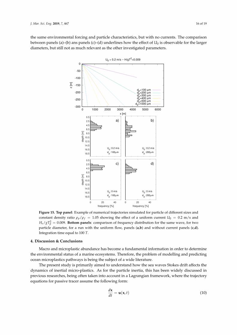
J. Mar. Sci. Eng. 2019, 7, 467 16 of 19

the same environmental forcing and particle characteristics, but with no currents. The comparisonbetween panels (a)–(b) ans panels (c)–(d) underlines how the effect of U0 is observable for the largerdiameters, but still not as much relevant as the other investigated parameters.

-300

-250

-200

-150

-100

-50

0

0 1000 2000 3000 4000 5000 6000

z [m

]

x [m]

U0 = 0.2 m/s -- H/gT2=0.009

dp=100 µmdp=200 µmdp=300 µmdp=400 µmdp=500 µm

dp=1000 µm

0.5

2.5

4.5

6.5

8.5

10.5

12.5

14.5

16.5

18.5

depth

[m

]

a)

dp: 100 m

U0: 0.2 m/s

b)

dp: 200 m

U0: 0.2 m/s

0 20 40

frequency [%]

0.5

2.5

4.5

6.5

8.5

10.5

12.5

14.5

16.5

18.5

depth

[m

]

c)

dp: 100 m

U0: 0 m/s

0 20 40

frequency [%]

d)

dp: 200 m

U0: 0 m/s

Figure 15. Top panel: Example of numerical trajectories simulated for particle of different sizes andconstant density ratio ρp/ρ f = 1.05 showing the effect of a uniform current U0 = 0.2 m/s andHs/gT2

p = 0.009. Bottom panels: comparison of frequency distribution for the same wave, for twoparticle diameter, for a run with the uniform flow, panels (a,b) and without current panels (c,d).Integration time equal to 100 T.

4. Discussion & Conclusions

Macro and microplastic abundance has become a fundamental information in order to determinethe environmental status of a marine ecosystems. Therefore, the problem of modelling and predictingocean microplastics pathways is being the subject of a wide literature.

The present study is primarily aimed to understand how the sea waves Stokes drift affects thedynamics of inertial micro-plastics. As for the particle inertia, this has been widely discussed inprevious researches, being often taken into account in a Lagrangian framework, where the trajectoryequations for passive tracer assume the following form:

dxdt

= u(x, t) (10)

J. Mar. Sci. Eng. 2019, 7, 467 17 of 19

Since plastic generally has a different density with respect to sea water, the present studyremoved such hypothesis, which may be no longer reasonable especially when heavy particlesare considered. Including the inertial effects extends Equation (10), leading to the trajectoriesexpressed by Equations (4) and (5). Our results seem to suggest that, for negatively buoyant particles,(e.g., ρp/ρ f > 1), the inertial effects dominate and the resulting horizontal distance of a single particleunder the effect of the sea wave drift can reach a maximum of few wavelengths (see Figures 7 and 8).Therefore, it is fundamental to take into account the inertial character of the debris, as this significantlyaffects the paths of negatively buoyant particles. The effect of a uniform current (U0) simply addsa displacement proportional to the current magnitude. On the other hand, as for plastic particlespositively buoyant, the Stokes drift proves to be an effective way of transport, since the particles tendto remain in a superficial layer where the drift is more intense. In this case the residence time of plasticdebris tends to increase indefinitely and, therefore, it is mandatory to consider other processes suchas biofouling, which has been shown to be able to modify the density and, ultimately, the settlingvelocity [21,22,38]. Another aspect that require further investigations is the the time evolution ofthe averaged vertical velocity w, which shows a transient regime characterized by an increment ofthe settling velocity. This can be relevant especially in shallow waters, where the combination ofparticles availability (e.g., sources of debris like rivers mouth etc.) and sea waves might acceleratethe deposition of heavy particles. As regards the vertical distributions resulting from the trajectoriescomputed according to Equations (4) and (5), interesting analogies with previous works can be pointedout: when random distributions for dp and ρp are considered, the frequencies tend to an exponentialprofile that is consistent with those highlighted by Kukulka et al. [12] and Enders et al. [20], evenif they relied on different models. It should be pointed out that at this stage, the model of Maxey& Riley [27] cannot be used for operational purposes. However, the second order Stokes waverepresents a reasonable choice for the wave model, since its validity is not bounded by the bottomdepth for common wave conditions. Then, the complexity of the marine environment implies thatseveral more effects need to be considered, such as (but not limited to) sub-grid turbulent diffusivity,biological processes that could affect the particle properties, and non linear effects related to breakingwaves [39,40].

These effects should be therefore implemented in regional models that aim to predict plasticdistribution is sea basins. However, Lagrangian numerical simulations that involve inertial propertiesrequire a computational effort more severe than that needed for standard Lagrangian models forpassive tracers. Indeed, the integration time step should be small compared to the Stokes time,otherwise the inertial response is not fully described. To overcome this limitation, it would be desirablea closure model, able to represent inertial effect through an effective diffusivity in analogy to thestandard closures for turbulent transport coefficient.

Finally, is is worth to mention that laboratory experiments are needed to further test the reliabilityof the analytical model. To this end, an experimental campaign has been recently kicked off at theDepartment of Civil, Chemical and Environmental Engineering of the University of Genoa, and willbe the focus of a future publication.

Author Contributions: A.S. developed the codes, run the numerical simulations, analyzed the results and wrotethe first draft of the paper; F.D.L. run the numerical simulations, analyzed the results and revised the paper; G.B.provided and analyzed the wave data, analyzed the results of the model and revised the paper.

Funding: This research was partially funded by the PADI Foundation 2018 grant www.padifoundation.org.

Conflicts of Interest: The authors declare no conflict of interest. The funders had no role in the design of thestudy; in the collection, analyses, or interpretation of data; in the writing of the manuscript, or in the decision topublish the results.

J. Mar. Sci. Eng. 2019, 7, 467 18 of 19

References

1. Thompson, R.C.; Swan, S.H.; Moore, C.J.; Vom Saal, F.S. Our Plastic Age. Philos. Trans. R. Soc. B 2009.[CrossRef] [PubMed]

2. Wilson, D.C.; Rodic, L.; Modak, P.; Soos, R.; Carpintero, A.; Velis, K.; Iyer, M.; Simonett, O. Global WasteManagement Outlook; UNEP: Nairobi, Kenya, 2015.

3. Jambeck, J.R.; Geyer, R.; Wilcox, C.; Siegler, T.R.; Perryman, M.; Andrady, A.; Narayan, R.; Law, K.L. Plasticwaste inputs from land into the ocean. Science 2015, 347, 768–771. [CrossRef] [PubMed]

4. Derraik, J.G. The pollution of the marine environment by plastic debris: A review. Mar. Pollut. Bull. 2002,44, 842–852. [CrossRef]

5. Kershaw, P.; Rochman, C. Sources, fate and effects of microplastics in the marine environment: Part 2of a global assessment. In Reports and studies-IMO/FAO/Unesco-IOC/WMO/IAEA/UN/UNEP Joint Groupof Experts on the Scientific Aspects of Marine Environmental Protection (GESAMP) Eng No. 93; InternationalMaritime Organization: London, UK, 2015.

6. Van Sebille, E.; Wilcox, C.; Lebreton, L.; Maximenko, N.; Hardesty, B.D.; Van Franeker, J.A.; Eriksen, M.;Siegel, D.; Galgani, F.; Law, K.L. A global inventory of small floating plastic debris. Environ. Res. Lett. 2015,10, 124006. [CrossRef]

7. Hidalgo-Ruz, V.; Gutow, L.; Thompson, R.C.; Thiel, M. Microplastics in the marine environment: a review ofthe methods used for identification and quantification. Environ. Sci. Technol. 2012, 46, 3060–3075. [CrossRef]

8. Bec, J. Fractal clustering of inertial particles in random flows. Phys. Fluids 2003, 15, L81–L84. [CrossRef]9. Maximenko, N.; Hafner, J.; Niiler, P. Pathways of marine debris derived from trajectories of Lagrangian

drifters. Mar. Pollut. Bull. 2012, 65, 51–62. [CrossRef]10. Zambianchi, E.; Trani, M.; Falco, P. Lagrangian transport of marine litter in the Mediterranean Sea.

Front. Environ. Sci. 2017, 5, 5. [CrossRef]11. Ballent, A.; Purser, A.; de Jesus Mendes, P.; Pando, S.; Thomsen, L. Physical transport properties of marine

microplastic pollution. Biogeosci. Discuss. 2012, 9. [CrossRef]12. Kukulka, T.; Proskurowski, G.; Morét-Ferguson, S.; Meyer, D.; Law, K. The effect of wind mixing on the

vertical distribution of buoyant plastic debris. Geophys. Res. Lett. 2012, 39. [CrossRef]13. Kukulka, T.; Brunner, K. Passive buoyant tracers in the ocean surface boundary layer: 1. Influence of

equilibrium wind-waves on vertical distributions. J. Geophys. Res. Oceans 2015, 120, 3837–3858. [CrossRef]14. Isobe, A.; Kubo, K.; Tamura, Y.; Kako, S.; Nakashima, E.; Fujii, N. Selective transport of microplastics and

mesoplastics by drifting in coastal waters. Mar. Pollut. Bull. 2014, 89, 324–330. [CrossRef] [PubMed]15. Liubartseva, S.; Coppini, G.; Lecci, R.; Creti, S. Regional approach to modeling the transport of floating

plastic debris in the Adriatic Sea. Mar. Pollut. Bull. 2016, 103, 115–127. [CrossRef] [PubMed]16. Zhang, H. Transport of microplastics in coastal seas. Estuar. Coast. Shelf Sci. 2017, 199, 74–86. [CrossRef]17. Liubartseva, S.; Coppini, G.; Lecci, R.; Clementi, E. Tracking plastics in the Mediterranean: 2D Lagrangian

model. Mar. Pollut. Bull. 2018, 129, 151–162. [CrossRef] [PubMed]18. Ourmieres, Y.; Mansui, J.; Molcard, A.; Galgani, F.; Poitou, I. The boundary current role on the transport and

stranding of floating marine litter: The French Riviera case. Cont. Shelf Res. 2018, 155, 11–20. [CrossRef]19. Jalón-Rojas, I.; Wang, X.H.; Fredj, E. On the importance of a three-dimensional approach for modelling the

transport of neustic microplastics. Ocean Sci. 2019, 15, 717–724. [CrossRef]20. Enders, K.; Lenz, R.; Stedmon, C.A.; Nielsen, T.G. Abundance, size and polymer composition of marine

microplastics greater then 10 µm in the Atlantic Ocean and their modelled vertical distribution. Mar. Pollut.Bull. 2015, 100, 70–81. [CrossRef]

21. Kooi, M.; van Nes, E.H.; Scheffer, M.; Koelmans, A.A. Ups and downs in the ocean: effects of biofouling onvertical transport of microplastics. Environ. Sci. Technol. 2017, 51, 7963–7971. [CrossRef]

22. Porter, A.; Lyons, B.P.; Galloway, T.S.; Lewis, C.N. The role of marine snows in microplastic fate andbioavailability. Environ. Sci. Technol. 2018. [CrossRef]

23. Arthur, C.; Baker, J.E.; Bamford, H.A. Proceedings of the International Research Workshop on the Occurrence,Effects, and Fate of Microplastic Marine Debris; University of Washington Tacoma: Tacoma, WA, USA, 2009.

24. Rios, L.M.; Moore, C.; Jones, P.R. Persistent organic pollutants carried by synthetic polymers in the oceanenvironment. Mar. Pollut. Bull. 2007, 54, 1230–1237. [CrossRef] [PubMed]

J. Mar. Sci. Eng. 2019, 7, 467 19 of 19

25. Fossi, M.C.; Panti, C.; Guerranti, C.; Coppola, D.; Giannetti, M.; Marsili, L.; Minutoli, R. Are baleen whalesexposed to the threat of microplastics? A case study of the Mediterranean fin whale (Balaenoptera physalus).Mar. Pollut. Bull. 2012, 64, 2374–2379. [CrossRef] [PubMed]

26. Peregrine, D. Interaction of water waves and currents. In Advances in Applied Mechanics; Elsevier: Amsterdam,The Netherlands, 1976; Volume 16, pp. 9–117.

27. Maxey, M.R.; Riley, J.J. Equation of motion for a small rigid sphere in a nonuniform flow. Phys. Fluids 1983,26, 883–889. [CrossRef]

28. Santamaria, F.; Boffetta, G.; Afonso, M.M.; Mazzino, A.; Onorato, M.; Pugliese, D. Stokes drift for inertialparticles transported by water waves. EPL (Europhys. Lett.) 2013, 102, 14003. [CrossRef]

29. DiBenedetto, M.H.; Ouellette, N.T.; Koseff, J.R. Transport of anisotropic particles under waves. J. Fluid Mech.2018, 837, 320–340. [CrossRef]

30. Khatmullina, L.; Isachenko, I. Settling velocity of microplastic particles of regular shapes. Mar. Pollut. Bull.2017, 114, 871–880. [CrossRef] [PubMed]

31. Mentaschi, L.; Besio, G.; Cassola, F.; Mazzino, A. Developing and validating a forecast/hindcast system forthe Mediterranean Sea. J. Coast. Res. 2013, 65, 1551–1556. [CrossRef]

32. Mentaschi, L.; Besio, G.; Cassola, F.; Mazzino, A. Problems in RMSE-based wave model validations.Ocean Model. 2013, 72, 53–58. [CrossRef]

33. Mentaschi, L.; Besio, G.; Cassola, F.; Mazzino, A. Performance evaluation of WavewatchIII in theMediterranean Sea. Ocean Model. 2015, 90, 82–94. [CrossRef]

34. LeMéhauté, B. An Introduction to Hydrodynamics and Water Waves; Springer: Berlin, Germany, 1976.35. Chubarenko, I.; Bagaev, A.; Zobkov, M.; Esiukova, E. On some physical and dynamical properties of

microplastic particles in marine environment. Mar. Pollut. Bull. 2016, 108, 105–112. [CrossRef]36. Kooi, M.; Reisser, J.; Slat, B.; Ferrari, F.F.; Schmid, M.S.; Cunsolo, S.; Brambini, R.; Noble, K.; Sirks, L.A.;

Linders, T.E.; et al. The effect of particle properties on the depth profile of buoyant plastics in the ocean.Sci. Rep. 2016, 6, 33882. [CrossRef] [PubMed]

37. Kumar, N.; Cahl, D.L.; Crosby, S.C.; Voulgaris, G. Bulk versus spectral wave parameters: Implicationson stokes drift estimates, regional wave modeling, and HF radars applications. J. Phys. Oceanogr. 2017,47, 1413–1431. [CrossRef]

38. Kaiser, D.; Kowalski, N.; Waniek, J.J. Effects of biofouling on the sinking behavior of microplastics.Environ. Res. Lett. 2017, 12, 124003. [CrossRef]

39. Deike, L.; Pizzo, N.; Melville, W.K. Lagrangian transport by breaking surface waves. J. Fluid Mech. 2017,829, 364–391. [CrossRef]

40. Pizzo, N.; Melville, W.K.; Deike, L. Lagrangian Transport by Nonbreaking and Breaking Deep-Water Wavesat the Ocean Surface. J. Phys. Oceanogr. 2019, 49, 983–992. [CrossRef]

c© 2019 by the authors. Licensee MDPI, Basel, Switzerland. This article is an open accessarticle distributed under the terms and conditions of the Creative Commons Attribution(CC BY) license (http://creativecommons.org/licenses/by/4.0/).