Seam Bias, Multiple-State, Multiple-Spell Duration Models and the Employment Dynamics of Disadvantaged Women

John C. Ham

University of Maryland, IFAU, IRP (UW-Madison) and IZA

Xianghong Li York University

Lara Shore-Sheppard

Williams College and NBER

Revised August 2011

This paper was previously circulated under the title “Analyzing Movements over Time in Employment Status and Welfare Participation while Controlling for Seam Bias using the SIPP.” We are grateful for comments received at the IRP Summer Research Workshop, as well as seminars at many universities and branches of the Federal Reserve Bank for suggestions that significantly improved the paper. Sandra Black, Richard Blundell, Mary Daly, Marcus Frölich, Soohyung Lee, Jose Lopez, Robert Moffitt, Geert Ridder, Melvin Stephens, Lowell Taylor and Tiemen Woutersen made very helpful remarks on an earlier draft. Eileen Kopchik provided, as usual, outstanding programming in deciphering the SIPP. This research has been supported by grants from the National Science Foundation (SES-0136928 and SES-0627968). Any opinions, findings and conclusions or recommendations in this material are those of the authors and do not necessarily reflect the views of the National Science Foundation. We are responsible for any errors. Contact information: John Ham (corresponding author), ham@econ.umd.edu, Department of Economics, 3105 Tydings Hall, University of Maryland, College Park, MD 20742, phone: (202) 380-8806, fax: (301) 405-3542; Xianghong Li, xli@econ.yorku.ca, Department of Economics, York University, 4700 Keele Street, Vari Hall 1068, Toronto, ON M3J 1P3, Canada, phone: (416) 736-2100 ext. 77036, fax: (416)736-5987; Lara Shore-Sheppard, Lara.D.Shore-Sheppard@williams.edu, Department of Economics, Williams College, 24 Hopkins Hall Drive, Williamstown, MA 01267, phone: (413) 597-2226, fax: (413) 597-4045.

ABSTRACT

Panel surveys generally suffer from “seam bias” - too few transitions observed within

reference periods and too many reported between reference periods. Seam bias is likely to affect

duration models severely since both the start date and the end date of a spell may be misreported. In

this paper we examine the employment dynamics of disadvantaged single mothers in the Survey of

Income and Program Participation (SIPP) while correcting for seam bias in reported employment

transitions. We develop parametric misreporting models for use in multi-state, multi-spell duration

analysis; the models are identified if misreporting parameters are the same for fresh and left-censored

spells of the same type. We extend these models to allow misreporting to depend on individual

characteristics and for a certain fraction of the sample never to misreport. Our models are

substantially more complex than the models used in previous studies of misclassification and

correspondingly offer a richer array of estimated policy effects. We compare our results to two

approaches used previously: i) using only data on the last month of reference periods and ii) adding a

dummy variable for the last month of the reference periods. We find that there are important

differences between our estimates and those obtained from ii), and very important differences

between our estimates and those obtained from i). We also consider three alternative models of

misreporting and are able to reject them based on aggregates of our micro data. We find that our

estimates are informative in terms of the effect of changes in demographic characteristics, macro

variables and policy variables on the expected duration of the different types of spells and on the

fraction of time employed in the short-run, medium-run and long-run.

1

1. Introduction

Many panel surveys suffer from “seam bias”. With seam bias, transitions or changes in status

within reference periods are underreported while too many transitions or changes are reported as

occurring between reference periods. In economics, this data problem was noted first by Czajka

(1983) for benefit receipt in the U.S. Income Survey Development Program. Since then seam effects

have been documented for various longitudinal surveys in many North American and European

countries, e.g. the Survey of Income and Program Participation (SIPP), the Current Population

Survey, the Panel Study of Income Dynamics (PSID), the Canadian Survey of Labour and Income

Dynamics, the European Community Household Panel Survey, and the British Household Panel

Survey.1 Lemaitre (1992) concludes that all current longitudinal surveys appear to be affected by

seam problems, regardless of differences in the length of recall periods or other design features. In

this paper we use multi-state, multi-spell duration models to examine the employment dynamics of

disadvantaged single mothers in the SIPP while correcting for seam bias in reported employment

status; note that the SIPP is the predominant data set used to analyze US anti-poverty policy.2 It is

straightforward to modify our approach to deal with seam bias in other longitudinal surveys. Finally,

our approach is equally applicable to structural and reduced form models of labor market transitions.

Seam bias plausibly would be most serious for estimating duration models, since it affects

the timing of transitions. Current approaches used in duration analysis to address seam bias can be

grouped into three general types. One approach, commonly used in the SIPP data, is to use only the

last month observation from each reference period (known as a “wave” in the SIPP),3 dropping the

three other months (e.g. Grogger 2004, Ham and Shore-Sheppard 2005, and Aaronson and Pingle

2006). Grogger is perhaps the strongest advocate of this approach. He argues that it is appropriate

because “most” transitions occur between waves (Grogger 2004, p. 673-674). However, as we show

in Section 4, approximately 50% of transitions occur between waves, i.e. in the last month and the

remaining 50% of the transitions occur within waves. Moreover, we show that it is easy to lose spells

and introduce significant measurement problems in terms of spell length and even in terms of

accurately separating one spell from another. Grogger (2004, p. 674) also motivates this approach by

arguing that “some of the within-wave transitions that exist are due to the SIPP imputation

procedures rather than changes in behavior (Westat, 2001).” However, the relevant question is

1 See Moore (2008) for a summary of seam bias research. 2 The Census Bureau, which collects the SIPP, has long recognized this problem and has attempted to reduce it in the SIPP, most recently by incorporating “dependent interviewing” procedures in the 2004 panel of the survey. Notwithstanding the adoption of such procedures, which explicitly link the wording of current interview questions to information provided in the preceding interview, seam bias continues to be a substantial problem in the SIPP (Moore 2008). 3 Each SIPP reference period has 4 months.

2

whether within-wave transitions are overrepresented in the imputed data relative to those in the last

month. We find that, in fact, approximately 50% of the transitions in the non-imputed data take

place in the last month, but about 81% of the transitions in the imputed data take place in the last

month. If in fact the SIPP imputation procedures have created artificial transitions, the empirical

evidence indicates any such transitions are much more concentrated in the last month instead of in

the other three within-wave months.

A second approach is to use the monthly data and to include a dummy variable for the last

month of the reference period (e.g. Blank and Ruggles 1996 and Fitzgerald 2004); the viability of this

approach depends on whether the problems introduced by seam bias can be effectively eliminated by

the use of a last month dummy. A third approach involves collapsing the employment indicator for

monthly data into an employment indicator for (four month) reference period. The reference period

employment indicator is set to 1 if the fraction of time respondents are employed or on welfare in

the reference period is above some (arbitrarily chosen) threshold (e.g. Acs, Philips, and Nelson 2003

and Ribar 2005). It is not obvious whether the appropriate threshold fraction of the reference period

with which to define the employment indicator is one-quarter, one-half, three-quarters or one.

Further, this approach is likely to result in the loss of short spells, and there are likely to be many

short employment spells for disadvantaged women (the population we study).

We propose a parametric approach to correct for seam bias in a multi-spell, multi-state

duration model and use maximum likelihood to estimate the model. The key assumption in our

approach is that respondents sometimes state that the employment status of the last month of the

reference period applies to all months in the reference period. This assumption represents the well-

known phenomenon (in the survey research literature) of telescoping of states (labor market status in

our study)4 or “reverse telescoping” of transitions.5 It is also consistent with the findings of previous

researchers on seam bias in economic data sets, such as Goudreau, Oberheu and Vaughan (1984),

who link AFDC income reporting in the Income Survey Development Program data to

administrative records.

We show that the misreporting parameters for fresh spells (i.e. spells beginning after the start

of the sample) are identified without restricting the form of the duration dependence, but that this is

not true for left-censored spells (i.e. spells in progress at the start of the sample). As a result, it is

tempting to base the analysis of disadvantaged women on fresh spells only, as do many studies in the

literature (e.g. Ham and Rea 1987, Baker and Rea 1998, Fitzenberger, Osikominu and Paul 2010, and

van den Berg and Vikström 2011), but this is a problematic approach for this population for several

4 See Sudman and Bradburn (1974), p.69. 5 See Lemaitre (1992).

3

reasons. First, Ham and LaLonde (1996) found that dropping left-censored spells caused an

important selection problem in their analysis of the effect of being offered the National Supported

Work training program on employment and unemployment transitions.6 Second, one cannot use the

same hazard function for left-censored spells as for fresh spells, and it is important to account for

left-censored spells in any policy simulation, because these spells dominate labor market histories for

disadvantaged women in the SIPP data. For example, even in month 30 of the various SIPP panels,

i.e. two and a half years after the start of the sampling period, left-censored spells still constitute over

sixty percent of both employment and non-employment spells. Another approach would be to

assume that there is no duration dependence in the left-censored spells, since, as we show below, this

will eliminate the identification problem. However, this assumption is strongly rejected in most, if

not all, previous studies of the labor market dynamics of disadvantaged women. Instead, we believe it

is much more reasonable to identify our model by assuming that left-censored employment (non-

employment) spells and fresh employment (non-employment) spells share the same misreporting

parameters.

Existing studies dealing with misclassification or misreporting due to seam bias consider

qualitatively different or simpler models than we do. Pischke (1995) proposes a method correcting

for seam bias in the SIPP for several different forms of misreporting when analyzing income

dynamics; since he is focusing on misreporting involving a continuous variable, his approach is

qualitatively different from ours. Considering limited dependent variable models, Card (1996) studies

the effects of unions on the structure of wages and estimates a static model that explicitly accounts

for misclassification errors in reported union status. Hausman, Abrevaya and Scott-Morton (1998)

deal with misclassification of dependent variables in static discrete-response models such as probit or

logit. Keane and Sauer (2009) allow for misclassification in a dynamic probit model describing female

labor force participation using the PSID. Their dynamic probit model can be viewed as a restrictive

version of our model, since it implicitly assumes that there is no duration dependence in either the

transition rate out of employment or the transition rate out of non-employment, in addition to

imposing cross-equation restrictions on the exit rates. Further, they do not explicitly model the

misclassification process. Two indications of how much richer our model is than models used in

previous work are i) none of the previous papers encounter an identification problem, and ii) if we

simplify our model to eliminate duration dependence (which leaves a model that is still more general

than a dynamic probit model), our identification problem disappears.7

6 Although Eberwein, Ham and LaLonde (1997) did not find such a selection problem in the effect of being offered participation, nor in the effect of actually participating, in the Job Training Partnership Act training program, the possibility of such selection clearly exists. 7 Also see Romeo (2001), who provides a data validation procedure consisting of multiple consistency checks

4

The closest study to ours is Abrevaya and Hausman (1999). Using the SIPP data, they

estimate a single-spell, single-state duration model where duration is measured with error (from all

possible sources). Compared to our approach, their nonparametric approach (the monotone rank

estimator) requires weaker assumptions because the misreporting process is not explicitly modeled.

Their approach is more general in terms of covering different forms of misreporting, but this

generality prevents users of this approach from being able to identify sufficient parameters to

calculate the effect of changing a policy variable (e.g. welfare benefits) on the expected duration of a

non-employment spell, and this effect is often crucial for policy analysis. Because Abrevaya and

Hausman (1999) investigate a single-spell model, they do not need to handle the issue that

mismeasurement in the duration of the current spell implies mismeasurement in the length of a

subsequent spell; in fact it is not clear how their approach can be applied to a multi-spell, multi-state

duration analysis. Indeed, our paper can be considered a response to Abrevaya and Hausman’s (1999)

concluding remarks (p.273): “In order to say anything about either the conditional expectation of y

(spell duration) given x or the baseline hazard function, the researcher would need to explicitly

model the mismeasurement process… Future research might consider specific mismeasurement

models for unemployment-spell data….” We not only accept this challenge, but we take it further by

solving this data problem in multi-spell, multi-state models.

Our goal here is to study the effect of policy and demographic variables on the labor market

dynamics of disadvantaged women. Using our estimates we can calculate the effect (and

corresponding standard error) of changing a policy variable on the fraction of time spent in

employment in the short-run, medium-run, and long-run, as well as the effect on the expected

duration of a spell. Since previous studies often calculate only the effect of a policy change on the

hazard functions or expected duration of a given type of spell, the effects we estimate are much more

informative for policy makers.8 We believe the added complexity of our approach is justified by the

much richer array of policy effects that it offers in comparison to the effects available previously.

Of course, as with any study using a parametric model, there is the issue of whether we have

the right model of misreporting behavior. To address this concern, we estimate several variants of

our base model. In addition, we offer several pieces of indirect evidence supporting our model. First,

the telescoping behavior underlying all of our misreporting models is exactly the type of behavior

that the 2004 revision of the SIPP aimed to minimize. Second, the findings of several previous for measuring the length of a single unemployment spell in the Current Population Survey and in the Computer Aided Telephone Interview/Computer Aided Personal Interview Overlap Survey. These procedures are data set and survey questionnaire specific, and cannot be straight-forwardly applied to SIPP or a multi-state, multi-spell duration model. 8 Eberwein, Ham and Lalonde (1997, 2002) calculate these effects for female participants in a JTPA training program, but do not calculate standard errors.

5

studies support our model of misreporting behavior and our finding of a higher misreporting

probability for minorities. Finally, we consider three alternative models of misreporting, but reject

them on the basis of results from aggregating our SIPP micro data. Thus, we consider a wide range

of possible misreporting behavior and find substantial support for our modeling strategy.

The paper proceeds as follows: In Section 2 we briefly discuss some of the large literature on

employment dynamics. In Section 3 we focus on the SIPP data and the extent of the seam bias

problem in it. In Section 4 we discuss the problems that occur when only the last month

observations in the SIPP data are used. We present our seam bias correction approach in Section 5.

We first outline the assumptions underlying our parametric approach. We then outline our approach

for estimating parametric single-spell duration models in the presence of seam bias and discuss

identification of these models. Finally, we consider correcting for seam bias when estimating multi-

spell, multi-state duration models.

We present our empirical results in Section 6. We find that there are important differences

between our seam bias estimates and those obtained with a last month dummy, and very important

differences between our seam bias estimates and those obtained using the last month data. We find

that our estimates are informative in terms of the effect of changes in demographic characteristics

and policy variables on the expected duration of the different types of spells and on the fraction of

time employed in the short-run, medium-run and long-run. We conclude the paper in Section 7.

2. The Employment Dynamics of Disadvantaged Women

In this paper we examine the employment dynamics of disadvantaged single mothers in the

SIPP while correcting for seam bias in reported employment status. Specifically, our target

population is single mothers with a high school education or less, a group that has been the focus of

much recent policy. We estimate monthly transition rates into and out of employment for the period

1986-1995, prior to the replacement of Aid to Families with Dependent Children (AFDC) with

Temporary Assistance to Needy Families (TANF). Transitions into and out of employment are of

crucial importance to policymakers, as they determine unemployment rates, poverty rates and the

overall well-being of low-income families. A clear understanding of employment dynamics is essential

for policymaking. For example, policymakers are likely to be very interested in the determinants of

employment duration, since short employment spells prevent disadvantaged individuals from

acquiring on-the-job human capital. The SIPP is particularly well-suited to estimate such models

because of its detailed monthly information on employment and program participation.

There have been relatively few North American studies focusing explicitly on employment

dynamics of the disadvantaged; exceptions are Aaronson and Pingle (2006), Eberwein, Ham and

6

LaLonde (1997) and Ham and LaLonde (1996). The related topic of welfare dynamics for less-

educated women has been examined in several U.S. and Canadian studies, e.g. Blank and Ruggles

(1996), Card and Hyslop (2005), and Keane and Wolpin (2002, 2007). Employment dynamics and

welfare dynamics will differ, as single mothers can work and collect welfare simultaneously, and can

certainly be out of employment and off welfare simultaneously. There is a large European literature

on employment dynamics for disadvantaged men and women, e.g. Blundell, Francesconi and Van der

Klaauw (2010), Cockx and Ridder (2003), Ham, Svejnar and Terrell (1998), Johansson and Skedinger

(2009), Micklewright and Nagy (2005), Ridder (1986) and Sianesi (2004).

Many of the above employment and welfare duration studies for Canada, the U.S. and the

UK used panel surveys. Consequently, these studies often were forced to confront (or ignore) the

seam bias problem. On the other hand, many of the continental European studies cited above used

administrative data. We would expect seam bias, and misreporting in general, to be less of a problem

in administrative data, but Chakravarty and Sarkar (1999) note that there appears to be seam bias at

the end of the month in their monthly administrative financial data. Further, Johansson and

Skedinger (2009) argue that there is misreporting in Swedish administrative data on disability status.

In future it would be interesting to investigate whether there is substantial seam bias in European

administrative labor market data; until this is done we believe our results will be of most use to

researchers studying the Canadian, U.S. and UK labor markets.

3. Seam Bias and the SIPP Data

Our primary data consist of the 1986-1993 panels of the SIPP. The SIPP was designed to

provide detailed information on incomes and income sources, as well as on the labor force and

program participation, of U.S. individuals and households. Our sample is restricted to single mothers

who have at most twelve years of schooling. Since we investigate employment status, we only

consider women between the ages of 16 and 55. 9 Although researchers investigating welfare

durations often smooth out one-month spells, we use the original data with all one-month spells

intact because employment status is often very unstable among low-educated women and it is

common for them to have very short employment and non-employment spells.10 Since we use state

9 Respondents are chosen based on their education and age at the beginning of the panel. If a single mother marries in the middle of the survey, we keep the observations before the marriage and treat the spell in progress at the time of marriage as right-censored. For this to be valid, we must treat marriage as an exogenous event; while in principle it would be interesting to allow for endogenous marriage, doing so is beyond the scope of the present paper. 10 Hamersma (2006) investigates a unique Wisconsin administrative data set containing information from all Work Opportunity Tax Credit (WOTC) and Welfare-to-Work (WtW) Tax Credit applications. The majority of WOTC-certified workers in Wisconsin are either welfare recipients or food stamp recipients. She finds that over one-third of certified workers have fewer than 120 annual hours of employment (job duration), while

7

level variables such as maximum welfare benefits, minimum wage rates, unemployment rates, and

whether the state obtained a welfare waiver and introduced positive incentives to leave welfare

(carrots) or negative incentives to leave (sticks), we exclude women from the smaller states which are

not separately identified in the SIPP.

The SIPP uses a rotation group design, with each rotation group consisting of about a

quarter of the entire panel, randomly selected. For each calendar month, members of one rotation

group are interviewed about the previous four months (the reference period or wave), and all

rotation groups are interviewed over the course of any four month period. Calendar months are thus

equally distributed among the months of the reference period. We call the four months within each

reference period month 1, month 2, month 3 and month 4. We will also refer to month 4 as the last month.

The rotation design guarantees that approximately 25% of transitions should occur in months 1, 2, 3

and 4 respectively. However, summary statistics show that for our sample 46% of all job transitions

(i.e. from non-employment to employment and vice-versa) are reported to occur in month 4, the last

month, and this percentage is far greater than the 25% one would expect. This seam effect, which

researchers have attributed to both too much change across waves and too little change within waves,

is observed for most variables in the SIPP (e.g. Young 1989, Marquis and Moore 1990, Ryscavage

1988 and Moore 2008).

To see how seam bias occurs in the SIPP, it is worth considering how the data are collected.

In the SIPP a respondent is first asked whether she had a job or business at any time during the

previous four-month period; if the answer is yes, the respondent is then asked whether she had a job

or business during all weeks of the period. Further questions are asked of individuals who report

some time employed and some time not employed. This serves to determine the timing of their

periods of employment and non-employment. For example, suppose an individual continues a spell

of non-employment into a given wave and does not have a job for months 1 and 2 of the new wave,

but she gets a job in month 3 that continues into month 4 of the wave. Given the interview structure,

under telescoping, this individual may report that she has a job for the whole wave based on the fact

she has a job in month 4, which is the month closest to (right before) the interview month. For this

particular example, a non-employment spell ending in month 2 of the current reference period will

be reported to end in month 4 of the previous reference period. Goudreau, Oberheu and Vaughan

another 29 percent of workers have fewer than 400 annual hours. Only a little over one-third of workers have annual employment of more than 400 hours. These administrative data show that a significant share of employment spells are less than one month among disadvantaged individuals. However, in our data it makes surprisingly little difference whether we smooth out the one-month spells.

8

(1984) document this as the most common type of misreporting behavior for AFDC benefit receipt

in the Income Survey Development Program.11

As discussed in the introduction, we estimate both fresh and left-censored spells jointly.

Table 1 provides mean characteristics and corresponding standard deviations (using the first month

of each spell) for our sample of employment and non-employment spells. Panel A shows that single

mothers in left-censored non-employment spells are usually more disadvantaged than those in fresh

non-employment spells. Specifically, those in left-censored non-employment spells are more likely to

be minorities, less likely to have a full twelve years of schooling, less likely to have had a previous

marriage, and are more likely to be disabled or have missing disability information than those in fresh

non-employment spells. Also, the single mothers in left-censored non-employment spells tend to

have more children, and their youngest children tend to be younger, compared to those in fresh non-

employment spells. The two groups are similar in terms of age. Panel B shows that those in left-

censored employment spells tend to be less disadvantaged than those in fresh employment spells.

Specifically, they are older, less likely to be minority group members, more likely to have twelve years

of schooling, more likely to have had a previous marriage, less likely to be disabled or have missing

disability information, and tend to have both fewer children and older children than those in fresh

employment spells.

4. Problems in Measuring Spells Using Only the Last Month Observations

As discussed in the introduction, a very common solution to the seam bias problem in the

SIPP data is to use only the last month observation from each wave, dropping the three other

months. In this section, we show that empirical evidence contradicts the two main reasons given for

using the last month data. In the SIPP, monthly data are imputed when a sample member either

refuses to be interviewed or is unavailable for that interview (and a proxy interview cannot be

obtained), or when someone who enters a sample household after the start of the panel leaves the

household during the reference period. 12 The Census Bureau indicates whether a monthly

observation is imputed using a variable INTVW, which equals 1 or 2 if a self or proxy interview is

obtained (and hence the data are not imputed) and 3 or 4 if the respondent refuses to be interviewed

or left, respectively (and hence the data are imputed). Using this variable, we compare the frequency

of transitions at the seam in the imputed and non-imputed data. Appendix Table A1 shows that

11 Their study is conducted by comparing respondents’ reports obtained from interviews with administrative record information. 12 All adults in sampled households at the start of the panel are considered original sample members and are followed to any new address. Someone entering a sample household after the start of the panel is interviewed as a member of the household, but not followed if he or she leaves. In that case, the remaining months of a reference period after the departure will be imputed.

9

approximately 50% of the transitions take place in month 4 in the non-imputed data, but about 81%

take place in month 4 in the imputed data.13 Hence, if imputation has created artificial transitions,

these transitions are much more concentrated in month 4 than in the first three months of a wave.

Next we show that almost one half of completed fresh spells are lost by using only the last

month data, and information on the timing of transitions that occur in months other than the last

month is lost, potentially introducing severe distortions to the true employment patterns. Under the

last month data approach, spells are constructed by acting as if we observe only the last month data

for each wave. When there is a status change from the previous month 4 to the current month 4,

month 4 of the current wave is coded as the end of a spell. Here we construct three examples

representative of our data to illustrate the problems that may arise when adopting this approach. In

these examples, which are shown in Figures 1.1 – 1.3, we let , ',U U E and 'E denote a fresh non-

employment spell, a left-censored non-employment spell, a fresh employment spell and a left-

censored employment spell, respectively. In each figure, the numbers above the line indicate the

survey months and the numbers below the line represent the reference period months. The first

example illustrated in Figure 1.1 assumes that a respondent has four spells. The first spell is a left-

censored non-employment spell ending in a month 1, the second is a fresh employment spell ending

in a month 3, the third is a fresh non-employment spell ending in another month 3, and the last spell

is a right-censored fresh employment spell. Using only the last month data, we would treat this

respondent’s work history as consisting of a left-censored non-employment spell lasting 32 months

and a right-censored employment spell lasting four months. We would lose both a two-month fresh

employment spell and a 24-month fresh non-employment spell. In addition, we would miscalculate

the spell length of both the left-censored and right-censored spells.

In the next example, shown in Figure 1.2, we keep everything else the same as in Figure 1.1

and only shift the ending point of the second spell to month 1 of a reference period. Now the second

fresh employment spell lasts for five months with a month 4 in the middle of the spell. For such a

case, using only last month data would not lead to the omission of the second and third spells, but

only to the miscalculation of the length of all four spells.

Finally, our last example assumes that a respondent has three spells as in Figure 1.3. The first

spell is a left-censored non-employment spell ending in month 3 of the first reference period; the

second is a completed fresh employment spell; and the third is a fresh non-employment spell

censored at the end of the sample. Using only last month data we would record this respondent’s

work history as a left-censored employment spell and a fresh non-employment spell. From this 13 The calculations in Table A1 are based on all transitions in the SIPP panels before we apply our sample selection criteria in Section 3. The fraction of transitions occurring in month 4 is slightly higher in this table than in our final sample.

10

example it is clear that we will lose all left-censored spells less than or equal to three months in length

by switching to the last month data. In addition, using the last month data may lead to both

miscalculating spell length and even misclassifying spell type for left-censored spells.

To recap, the above three examples show that by using only the last month data, we could

lose some spells, miscalculate the length of spells, and misclassify the spell type. The problem is more

severe with short spells that are less than four months duration and that do not cover a month 4.

Further, it is clear that in general using only the last month observations will lead to an overestimate

of the length of left-censored spells. However, for fresh spells, using only the last month data may

underestimate or overestimate the length of an observed fresh spell, since both the start and end of a

fresh spell could be mismeasured.

Of course, the above three examples compare the last month data to the true duration data,

while in practice we do not know the true duration of spells. Thus, the relevant comparison is the last

month data versus the monthly data contaminated by seam bias. Here we would make two points.

First, even in the presence of seam bias we still observe many short spells in our data, including spells

falling between two interviews as in Figure 1.1.14 If some short spells are omitted due to seam bias,

switching to using only the last month data certainly will not help us capture those omitted short

spells. Second, the implications of Figures 1.1 to 1.3 also hold for comparisons of spells based on the

monthly data contaminated by seam bias and spells based on only the last month observations from

the contaminated data.

To shed more light on the comparison between the contaminated monthly data and the last

month only data, we examine the number of completed spells and the empirical survivor functions

for each data type. First, comparing the number of completed spells (which provide the empirical

identification for the parameters of the hazard functions), we find that shifting from using monthly

data to the last month data results in the loss of about 47% of fresh employment spells, 48% of fresh

non-employment spells, 20% of left-censored employment spells, and 18% of left-censored non-

employment spells. Second, when considering all spells (completed spells and right-censored spells),

shifting from monthly data to the last month data still results in the loss of 34 to 35 percent of fresh

spells. (See Online Appendix Table A2, which presents distributions of spell length and total number

of spells of monthly data versus last month data for all spells.15) However, it is difficult to ascertain

the effect of using the last month data on spell lengths from Table A2 because of the right-censored

14 An accurate measure of the frequency with which individuals fail to report short spells can only be obtained from matched administrative-survey data, which we do not have for this sample. 15 The numbers of spells in the table are larger than those in Table 1 because here we have not imposed the selection criteria discussed in Section 3. Our Online Appendix is found at http://dept.econ.yorku.ca/~xli/ HomePage_files/appendix_seam_bias_hls.pdf.

11

spells. Instead, we investigate the empirical survivor functions. Online Appendix Figures A.1 and

A.2 show that using only the last month data will increase the estimated survivor function for left-

censored employment and non-employment spells by a considerable amount. Online Appendix

Figures A.3 and A.4 show that this phenomenon is even more pronounced for fresh employment

and non-employment spells.

These calculations indicate that shifting from the contaminated (by seam bias) data to only

the last month data leads to omitting spells and overestimating the spell length. Moreover, using only

the last month data will lead to a loss of efficiency since data from three-fourths of the months are

being discarded, and nearly 55 percent of transitions occur in these months.

5. Correcting for Seam Bias

In this section we describe a model of misreporting behavior that allows us to address the

estimation problems caused by seam bias. We first develop a single spell monthly discrete time

duration model for employment (non-employment) spells with three extra parameters that capture

the misreporting of transitions. Under reasonable assumptions, we show that we can identify these

parameters in our model for fresh employment spells, but cannot identify a separate set of

misreporting parameters for left-censored employment spells without restricting the form of the

duration dependence. This identification problem has not arisen in previous empirical studies

considering misclassification, indicating the greater richness of our econometric model. To identify

the model, we thus assume that fresh and left-censored employment (non-employment) spells share

the same misreporting parameters. We then consider the extension to a multi-state multi-spell

duration model. Since the model is significantly overidentified given the equality constraints of

misreporting parameters, we are able to consider several extensions of the model. Finally, we

consider three alternative models of misreporting, but reject them on the basis of aggregating micro

data from the SIPP.

5.1 Notation

We first set up our notation before discussing our assumptions. Let ,obsM j l represent

a spell reported to end in month j of reference period (wave) l .16 Note that ,obsM j l could be

contaminated by seam bias. Further, let ,trueM j l represent the fact that a spell truly ended in

month j of reference period l . The variable j in obsM and trueM assumes five possible values: 1,

16 The end of a spell can occur either because a transition took place or because the individual reached the end of the sample period.

12

2, 3, 4, or 0, where j 1, 2, 3 or 4 indicates a transition in months 1, 2, 3 or 4, respectively, and

0j indicates a right-censored spell ending with the survey. For our sample l takes on the values

from 1 to L , where L is the number of waves, which depends on the specific SIPP panel being

used.17 For example, (4, 4)obsM indicates that a transition was reported to have occurred in

month 4 of reference period 4, while (3,5)trueM denotes that the transition actually occurred in

month 3 of reference period 5.

5.2 Behavioral Assumptions

Given the interview structure described in section 3 above, documented empirical evidence

of seam bias in SIPP variables, and previous research on survey and administrative data, we make the

following main assumption: respondents sometimes report the employment status of month 4 for all

months in the reference period, which has the effect of moving a transition that actually occurred in

months 1, 2 or 3 of a given reference period to month 4 of the previous reference period. In terms of

labor market state, this reflects the well-known phenomenon of telescoping (respondents recall that

previous states are the same as the state in the current period, Sudman and Bradburn 1974, p.69),

while in terms of transitions, it reflects the well-known phenomenon of “reverse telescoping”

(respondents recall transitions as having occurred more distantly than in fact was the case, Lemaitre

1992). This is also similar to the third type of household behavior considered by Pischke (1995,

p.824), where he assumes that respondents report their permanent income (but not transitory income)

in month 4 as applying to all months in the wave. We make the following five assumptions for each

interview:

A1) the respondents report all transitions that occurred during reference period l as occurring either

in the true month or month 4 of reference period 1l ;

A2) if a respondent reports that a transition happened in months 1, 2 or 3 of a reference period, it is

a truthful report;

A3) a respondent reports a transition that actually occurred in months 1, 2 or 3 of reference period l

as taking place in month 4 of reference period 1l with some pre-specified but unknown

probabilities 1 2, and 3 respectively; i.e. the probability of misreporting does not depend on the

reference period or current duration in the spell.

A4) if a transition truly happened in month 4 of a reference period, the respondent reports it as

occurring in that month; and

17 There are seven waves in the 1986 and 1987 panels, six in the 1988 panel, eight in the 1990 and 1991 panels, ten in the 1992 panel, and nine in the 1993 panel.

13

A5) the true transition rate for a given duration does not depend on the reference period month, j ,

i.e. duration is not affected by whether one is in month one, two, three or four of the reference

period.18

Given these behavioral assumptions,19 we have the following conditional probabilities:

( , ) ( , ) 0, j 1, 2, 3;obs trueP M j l M j l (5.1)

(4, 1) ( , ) , j 1, 2, 3;obs truejP M l M j l (5.2)

(4, ) (4, ) 1 obs trueP M l M l and (5.3)

(0, ) (0, ) 1 .obs trueP M l M l (5.4)

5.3 Correcting for Seam Bias in a Single Spell Model

To illustrate the method in the simplest way, we first explore the problem involving a single

spell of employment. We define the hazard function for individual i as

1

( | ( ), )1 exp ( ) ( )i i

i i

t X th t X t

, (5.5)

where t denotes current duration, ( )h t denotes duration dependence, denotes the calendar time

of the start of the spell and ( )iX t denotes a (possibly) time changing explanatory variable.

Further, i denotes unobserved heterogeneity, and following Heckman and Singer (1984b), we

assume that it is i.i.d. across i and is drawn from a discrete distribution function with points of

support 1 1,..., ,J J and associated probabilities 1 1,..., Jp p and1

1

1 .J

J kk

p p

For example, if a

spell lasts K months, the contribution to the likelihood function for individual i is

1

1 1

( | ( ), ) (1 ( | ( ), ))J K

i j i i j i i jj t

L K p K X K t X t

. (5.6)

For notational simplicity, we drop the individual subscript i in the following discussion.

Based on our behavioral assumptions, it is straightforward to derive the likelihood function

given that we observe ,obsM m l , and the reported length of the spell, obsdur , both of which

18 This assumption is the consequence of the survey design. For ease of interviewing, the entire sample is randomly split into four rotation groups, and one rotation group (1/4 of the sample) is interviewed each calendar month. Each rotation group in a SIPP panel is interviewed once every four months about employment and program participation during the previous four months. 19 Our assumptions rule out the possibility that individuals forget about very short spells that fall between two interviews. However, without administrative data linked to the SIPP data, we have no way of verifying the validity of this assumption.

14

potentially have been contaminated by seam bias.20 The contribution to the likelihood function for a

completed spell of observed length K that ends in months 1, 2, 3, or 4 of reference period l is

given by (derivations are provided in Appendix 1):

11, , 1 ( )obs obsP M l dur K L K ; (5.7)

22, , 1obs obsP M l dur K L K ; (5.8)

33, , = (1 )obs obsP M l dur K L K and (5.9)

1 2 34, , 1 2 3 .obs obsP M l dur K L K L K L K L K (5.10)

A natural question to ask is whether the model is identified without restricting the form of

the duration dependence. In the next section we show that a model with only duration dependence

and misreporting parameters is (over) identified for fresh employment and non-employment spells,

but is not identified for left-censored employment and non-employment spells, assuming that each

type of spell has entirely different misreporting and duration dependence parameters. However, we

also show that all parameters are identified if we assume that left-censored employment (non-

employment) spells and fresh employment (non-employment) spells share the same misreporting

parameters, and thus we make this assumption below. Indeed, we show that given this assumption

the model is overidentified.

5.4 Identification of Duration Dependence and Seam Bias Parameters in Single Spell

Data

Adding seam bias correction parameters to the model raises the question of whether this will

hinder identification of the model without further restrictions. We address this question for a model i)

without explanatory variables and ii) without unobserved heterogeneity. Assumption i) is harmless in

the sense that we can always cross stratify the data by cells determined by the explanatory variables.

Assumption ii) reflects that there is a gap in the theoretical literature on nonparametric identification

of discrete time models (or continuous time models where outcomes are discretely observed). The

only study we are aware of in this area – Hausman and Woutersen (2010) – is not applicable for our

case since they look at non-parametric identification of duration dependence with covariates while

allowing for unspecified unobserved heterogeneity, i.e. they do not estimate the parameters of the

unobserved heterogeneity distribution but instead treat them as nuisance parameters.

20 Here we assume that seam bias affects only the end date, and not the start date, of a spell. We relax this assumption when we consider multiple spell data.

15

Thus we do not consider unobserved heterogeneity when investigating identification issues

in our study. We show that the seam bias correction parameters cannot be identified in the left-

censored spells without restricting the form of the duration dependence, although this problem does

not arise in the fresh spells. We resolve the identification problem by assuming that the fresh and

left-censored spells share the same misreporting parameters, since this seems much more reasonable

than restricting the duration dependence in the left-censored spells. After imposing this equality

assumption, we find that our model is significantly overidentified, and we are able to consider several

extensions of the misreporting model.21

5.4.1 Identification with Fresh Spell Data

At first glance, it may appear that we have to restrict the form of the duration dependence to

identify our model. However, this is not the case, at least for fresh spells. As noted above, we

consider a model for employment spells with duration dependence but no explanatory variables and

no unobserved heterogeneity, so that the only parameters are the hazard function for each duration

month t and the misreporting probabilities. (The argument for non-employment spells is identical.)

One can estimate the parameters of this simplified model by comparing sample moments and their

probability limits, which we will refer to as population moments.

Let ( )jm k denote the empirical hazard function for spells ending at duration k in reference

month ,j j 1, 2, 3, 4. These are our sample moments; denote their population counterparts by

( ).jp k To obtain these population moments, first assume that in the population there are tN , 1tN ,

2tN , and 3tN individuals having current durations equal to t , 1t , 2t , and 3t , respectively

in month 4 over all reference periods. ( tN , 1tN , 2tN , and 3tN may be thought of as being large

but finite for now, as they will drop out of the population moments below.)

Using the terminology of the duration literature, tN , 1tN , 2tN , and 3tN represent the

total number of individuals at risk at durations t , 1t , 2t , and 3t respectively in month 4. As

discussed in Section 5.2, we assume that seam bias only occurs when transitions in months 1, 2, and

3 of the following reference period are heaped into the current month 4, so tN , 1tN , 2tN , and

3tN are not contaminated by seam bias. For month 1, in large samples the number of individuals

who actually enter month 1 at duration t is 1 1 1tN t . This is the number of individuals at

risk at duration t in month 1, i.e. the difference between the number entering the previous month 4

21 Further, we found that adding a flexible specification for the unobserved heterogeneity in estimation did not cause any empirical identification problems for our basic or extended misreporting models.

16

at duration 1t and the number who leave in the previous month 4 at duration 1t . However,

note that the number observed to be at risk consists of those actually at risk minus the sum of:

1. The number of individuals who actually left in month 1 at duration t but were observed to exit

in the previous month 4 due to seam bias, 1 11 1tN t t ;

2. The number of individuals who actually left in month 2 at duration 1t but were observed to

exit in the previous month 4 due to seam bias 1 21 1 1 1tN t t t ;

and

3. The number of individuals who actually left in month 3 at duration 2t but were observed to

exit in the previous month 4 due to seam bias

1 31 1 1 1 1 2tN t t t t .

Of those actually at risk in month 1, in large samples a fraction t actually leave, but only a

fraction 11t are observed to have left in month 1, and the rest 1t were reported to

have left in the previous month 4 due to seam bias. Thus the number observed leaving

equals 1 11 1 1tN t t . Given this, we can easily formulate the first population

moment condition for the fraction observed to leave in month 1 at duration t (after deleting the

common factor 1 1 1tN t from both the numerator and denominator) as

11

1 2 3

1( ) .

1 1 1 1 1 1 2

tp t

t t t t t t

(5.11)

For month 2, the expected number of individuals who actually enter month 2 at duration t is

2 1 2 1 1tN t t . Due to seam bias, the number observed to be at risk in month 2

consists of those actually at risk minus the sum of

1. those who actually left in month 2 at duration t but were observed to exit in the previous

month 4, 2 21 2 1 1tN t t t ; and

2. those who actually left in month 3 at duration 1t but were observed to exit in the previous

month 4, 2 31 2 1 1 1 1tN t t t t .

Because of seam bias, the number observed to leave at duration t in month 2 equals

2 21 2 1 1 1tN t t t . Thus, our second population moment (after

17

canceling out the common factor 2 1 2 1 1tN t t from both the numerator and

denominator) is

2 ( )p t

2

2 3

1.

1 1 1

t

t t t

(5.12)

For month 3, the number of individuals who actually entered month 3 at duration t is

3 1 3 1 2 1 1tN t t t . Due to seam bias, the number observed to be at risk

in month 3 consists of those actually at risk minus those who actually left in month 3 at duration t

but were observed to exit in the previous month 4,

3 31 3 1 2 1 1tN t t t t . The number observed leaving equals

3 31 3 1 2 1 1 1tN t t t t . Thus, our third population moment

(after deleting the common factor 3 1 3 1 2 1 1tN t t t from both the

numerator and denominator) is

33

3

1( ) .

1

tp t

t

(5.13)

For month 4, under our assumptions the number of individuals who actually (and were observed

to) enter month 4 at duration t is tN . The number of individuals who actually leave in month 4 at

duration t equals tN t . However, due to seam bias, we also observe leaving in month 4

1. 11 1tN t t individuals who actually left in month 1 of the next reference

period but reported leaving in month 4,

2. 21 1 1 2tN t t t individuals who actually left in month 2 of the

next reference period but reported leaving in month 4 and

3. 31 1 1 1 2 3tN t t t t individuals who actually left in

month 3 of the next reference period but reported leaving in month 4.

The number of individuals observed leaving in month 4 equals the sum of tN t and the three

terms above. Thus after canceling out tN from both the numerator and denominator we have

4 1 2

3

( ) 1 1 1 1 1 2

1 1 1 1 2 3 .

p t t t t t t t

t t t t

(5.14)

18

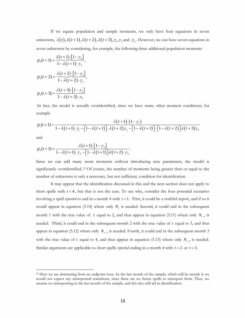
If we equate population and sample moments, we only have four equations in seven

unknowns, 1 2, 1 , 2 , 3 , ,t t t t and 3 . However, we can have seven equations in

seven unknowns by considering, for example, the following three additional population moments

33

3

1 1( 1) ,

1 1

tp t

t

33

3

2 1( 2) ,

1 2

tp t

t

33

3

3 1( 3)

1 3

tp t

t

.

In fact, the model is actually overidentified, since we have many other moment conditions; for

example

11

1 2 3

1 1( 1)

1 1 1 1 2 1 1 1 2 3

tp t

t t t t t t

and

22

2 3

1 1( 1)

1 1 1 1 2

tp t

t t t

.

Since we can add many more moments without introducing new parameters, the model is

significantly overidentified. 22 Of course, the number of moments being greater than or equal to the

number of unknowns is only a necessary, but not sufficient, condition for identification.

It may appear that the identification discussed in this and the next section does not apply to

short spells with 4t , but that is not the case. To see why, consider the four potential scenarios

involving a spell reported to end in a month 4 with 1t . First, it could be a truthful report, and if so it

would appear in equation (5.14) where only tN is needed. Second, it could end in the subsequent

month 1 with the true value of t equal to 2, and thus appear in equation (5.11) where only 1tN is

needed. Third, it could end in the subsequent month 2 with the true value of t equal to 3, and thus

appear in equation (5.12) where only 2tN is needed. Fourth, it could end in the subsequent month 3

with the true value of t equal to 4, and thus appear in equation (5.13) where only 3tN is needed.

Similar arguments are applicable to short spells reported ending in a month 4 with 2t or 3t .

22 Here we are abstracting from an endpoint issue. In the last month of the sample, which will be month 4, we would not expect any misreported transitions, since there are no future spells to misreport from. Thus, we assume no misreporting in the last month of the sample, and this also will aid in identification.

19

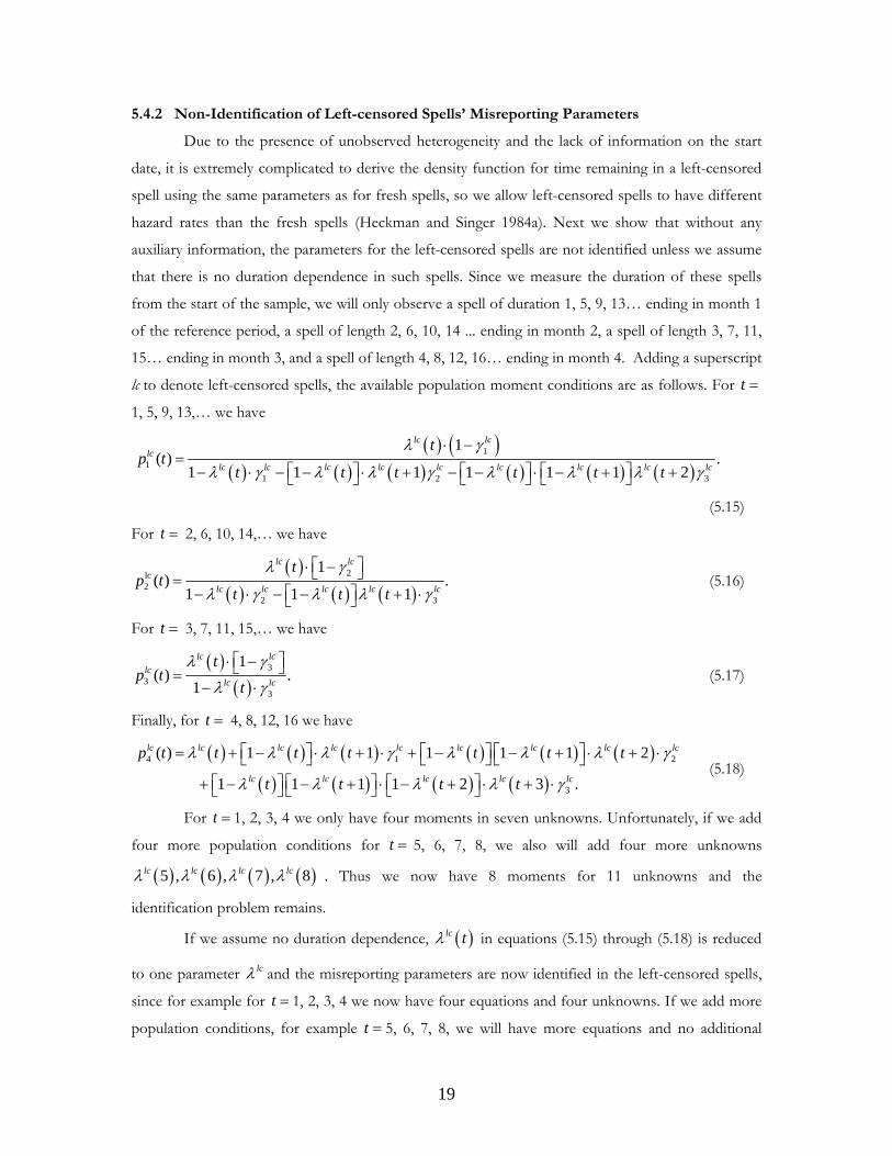
5.4.2 Non-Identification of Left-censored Spells’ Misreporting Parameters

Due to the presence of unobserved heterogeneity and the lack of information on the start

date, it is extremely complicated to derive the density function for time remaining in a left-censored

spell using the same parameters as for fresh spells, so we allow left-censored spells to have different

hazard rates than the fresh spells (Heckman and Singer 1984a). Next we show that without any

auxiliary information, the parameters for the left-censored spells are not identified unless we assume

that there is no duration dependence in such spells. Since we measure the duration of these spells

from the start of the sample, we will only observe a spell of duration 1, 5, 9, 13… ending in month 1

of the reference period, a spell of length 2, 6, 10, 14 ... ending in month 2, a spell of length 3, 7, 11,

15… ending in month 3, and a spell of length 4, 8, 12, 16… ending in month 4. Adding a superscript

lc to denote left-censored spells, the available population moment conditions are as follows. For t

1, 5, 9, 13,… we have

1

1

1 2 3

1 ( ) .

1 1 1 1 1 1 2

lc lc

lc

lc lc lc lc lc lc lc lc lc

tp t

t t t t t t

(5.15)

For t 2, 6, 10, 14,… we have

2lc2

2 3

1( ) .

1 1 1

lc lc

lc lc lc lc lc

tp t

t t t

(5.16)

For t 3, 7, 11, 15,… we have

3

33

1( ) .

1

lc lc

lclc lc

tp t

t

(5.17)

Finally, for t 4, 8, 12, 16 we have

4 1 2

3

( ) 1 1 1 1 1 2

1 1 1 1 2 3 .

lc lc lc lc lc lc lc lc lc

lc lc lc lc lc

p t t t t t t t

t t t t

(5.18)

For t 1, 2, 3, 4 we only have four moments in seven unknowns. Unfortunately, if we add

four more population conditions for t 5, 6, 7, 8, we also will add four more unknowns

5 , 6 , 7 , 8lc lc lc lc . Thus we now have 8 moments for 11 unknowns and the

identification problem remains.

If we assume no duration dependence, lc t in equations (5.15) through (5.18) is reduced

to one parameter lc and the misreporting parameters are now identified in the left-censored spells,

since for example for t 1, 2, 3, 4 we now have four equations and four unknowns. If we add more

population conditions, for example t 5, 6, 7, 8, we will have more equations and no additional

20

unknowns. Thus under the assumption of no duration dependence, the left-censored spell hazard

functions and misreporting parameters are also overidentified.

Since assuming that there is no duration dependence in left-censored spells runs contrary to

most empirical evidence on such spells for disadvantaged women, we must find a more reasonable

assumption with which to identify our model. Note that if we assume the fresh employment spells

and the left-censored employment spells share the same misreporting parameters, i.e. lck k , for

k 1, 2, 3, the model becomes overidentified (as in Section 5.4.1). We thus impose these constraints

on employment spells and the analogous constraints for non-employment spells to identify the

model that includes left-censored spells.23

In the introduction we noted that Keane and Sauer (2009) investigated misclassification

within a dynamic probit model of female labor participation without encountering identification

problems. Note that our identification problem is consistent with their lack of an identification

problem because a dynamic probit model is a restricted version of our model, where one restriction

implicit in a dynamic probit model is the absence of duration dependence. The difference in the

identification problems between their study (and previous studies in the literature) and ours occurs

because our model is substantially richer than existing models dealing with misclassification.

5.5 Correcting for Seam Bias in a Multiple-Spell Model

In a multiple-spell discrete time duration model, correcting for seam bias complicates the

likelihood function dramatically since adjusting a response error in one spell involves shifting not

only the end of the current spell but also the start of the subsequent spell. This is a serious problem

as respondents in our sample have up to seven spells and a respondent can have several spells ending

in month 4 in her history. We continue to use separate hazard functions for the left-censored spells,

and we let the employment spells (non-employment spells), both left-censored and fresh, share one

set of seam bias parameters, 1 2,E E , and 3E ( 1 2,U U and 3

U ) as defined in equation (5.2).24 As

defined in Section 4, we let 'U and U represent left-censored and fresh non-employment spells

respectively, and let 'E and E represent left-censored and fresh employment spells respectively. We

follow standard practice and specify the unobserved heterogeneity corresponding to these four types

of spells through a vector ' '( , , , )U U E E , and assume that is distributed independently

across individuals and is fixed across spells for a given individual. Following McCall’s (1996)

23 Note that this identification problem would disappear if we had information on (and used) the actual start date of the left-censored spells. 24 As we show in the previous section, we cannot let the seam bias parameters differ between left-censored and fresh spells of the same type.

21

multivariate generalization of the Heckman-Singer (1984b) approach, we let follow a discrete

distribution with points of support 1 2, ,..., J , (where, e.g., 1 1 '1 1( , , ,U U E '1)E ) and associated

probabilities 1 2, ,..., Jp p p respectively, where1

1

1 .J

J kk

p p

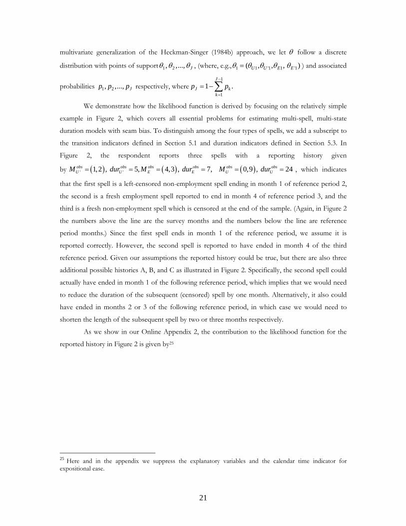
We demonstrate how the likelihood function is derived by focusing on the relatively simple

example in Figure 2, which covers all essential problems for estimating multi-spell, multi-state

duration models with seam bias. To distinguish among the four types of spells, we add a subscript to

the transition indicators defined in Section 5.1 and duration indicators defined in Section 5.3. In

Figure 2, the respondent reports three spells with a reporting history given

by ' '1,2 , 5, 4,3 , 7,obs obs obs obsU U E EM dur M dur 0,9 , 24obs obs

U UM dur , which indicates

that the first spell is a left-censored non-employment spell ending in month 1 of reference period 2,

the second is a fresh employment spell reported to end in month 4 of reference period 3, and the

third is a fresh non-employment spell which is censored at the end of the sample. (Again, in Figure 2

the numbers above the line are the survey months and the numbers below the line are reference

period months.) Since the first spell ends in month 1 of the reference period, we assume it is

reported correctly. However, the second spell is reported to have ended in month 4 of the third

reference period. Given our assumptions the reported history could be true, but there are also three

additional possible histories A, B, and C as illustrated in Figure 2. Specifically, the second spell could

actually have ended in month 1 of the following reference period, which implies that we would need

to reduce the duration of the subsequent (censored) spell by one month. Alternatively, it also could

have ended in months 2 or 3 of the following reference period, in which case we would need to

shorten the length of the subsequent spell by two or three months respectively.

As we show in our Online Appendix 2, the contribution to the likelihood function for the

reported history in Figure 2 is given by25

25 Here and in the appendix we suppress the explanatory variables and the calendar time indicator for expositional ease.

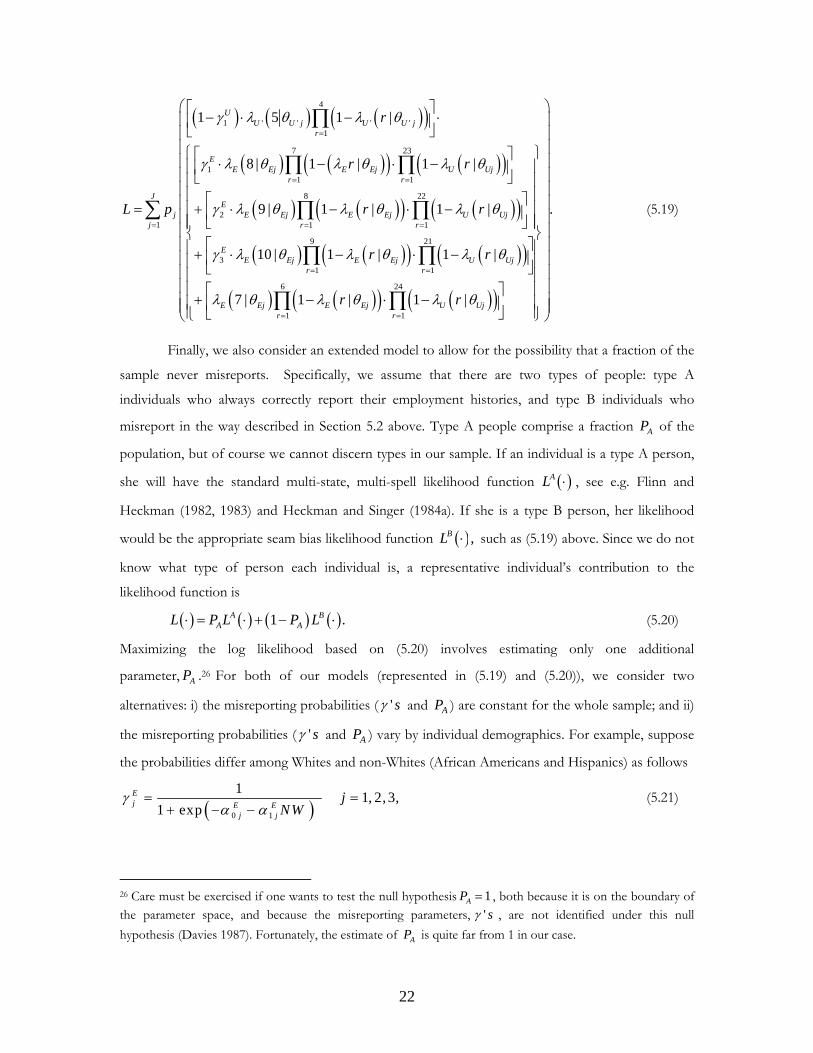
22

4

1 ' ' ' '1

7 23

11 1

8 22

21 1 1

9 21

31 1

1 5 1 |

8 | 1 | 1 |

9 | 1 | 1 |

10 | 1 | 1 |

7 | 1

UU U j U U j

r

EE Ej E Ej U Uj

r r

JE

j E Ej E Ej U Ujj r r

EE Ej E Ej U Uj

r r

E Ej

r

r r

L p r r

r r

6 24

1 1

.

| 1 |E Ej U Ujr r

r r

(5.19)

Finally, we also consider an extended model to allow for the possibility that a fraction of the

sample never misreports. Specifically, we assume that there are two types of people: type A

individuals who always correctly report their employment histories, and type B individuals who

misreport in the way described in Section 5.2 above. Type A people comprise a fraction AP of the

population, but of course we cannot discern types in our sample. If an individual is a type A person,

she will have the standard multi-state, multi-spell likelihood function AL , see e.g. Flinn and

Heckman (1982, 1983) and Heckman and Singer (1984a). If she is a type B person, her likelihood

would be the appropriate seam bias likelihood function ,BL such as (5.19) above. Since we do not

know what type of person each individual is, a representative individual’s contribution to the

likelihood function is

1 .A BA AL P L P L (5.20)

Maximizing the log likelihood based on (5.20) involves estimating only one additional

parameter, AP .26 For both of our models (represented in (5.19) and (5.20)), we consider two

alternatives: i) the misreporting probabilities ( ' s and AP ) are constant for the whole sample; and ii)

the misreporting probabilities ( ' s and AP ) vary by individual demographics. For example, suppose

the probabilities differ among Whites and non-Whites (African Americans and Hispanics) as follows

0 1

11, 2, 3,

1 expEj E E

j j

jNW

(5.21)

26 Care must be exercised if one wants to test the null hypothesis 1AP , both because it is on the boundary of the parameter space, and because the misreporting parameters, ' s , are not identified under this null

hypothesis (Davies 1987). Fortunately, the estimate of AP is quite far from 1 in our case.

23

where NW is a dummy variable equal to 1 if an individual is non-White and zero otherwise. We use

an analogous specification for non-employment spells.27

5.6 Alternative Misclassification Schemes

Of course, there is the possibility that the transitions are misclassified in a way that differs

from our approach described above. Here we consider several other possibilities which we argue can

be rejected based on aggregates of our micro data. The first possibility we consider is: some of the

month 1 transitions are pushed into month 2, some of the month 2 transitions are pushed into

month 3, and some of the month 3 transitions are pushed into month 4, but none of the month 4

transitions are pushed into the next reference period (because it is the last month in the reference

period). If 50% of the transitions in months 1, 2 and 3 are pushed to the next month, then we would

see 12.5 % of the transitions in month 1, 25% in month 2, 25% in month 3, and 37.5% in month 4.

Alternatively, suppose 75% of the transitions get pushed out of months 1, 2, and 3. Then we would

see 6.25% of the transitions in month 1, 25% in month 2, 25% in month 3, and 43.75% in month 4.

In either case, month 1 should have a considerably smaller proportion of the transitions than months

2 and 3, and month 4 should have a considerably larger proportion of the transitions than months 2

and 3. However, in our final sample, months 1, 2, 3, and 4 have 16.57%, 19.08%, 18.49%, and

45.86% of the employment/non-employment transitions respectively, which is clearly inconsistent

with this alternative model. (Note that our proposed model is consistent with this pattern).

Secondly, we consider the possibility that some of the transitions in month 1 of the

reference period 1l are pushed back into month 4 of reference period l . (Recall that month 1 of

the reference period 1l is the interview month for reference period l .) If this is the only source of

misclassification, then the pattern should be similar to the scheme above: about 25% of the observed

transitions are reported in months 2 and 3, a smaller proportion of transactions are reported in

month 1, and a larger proportion in month 4. This model would also be rejected by the summary

statistics presented in the previous paragraph.

A third possible explanation of the aggregate transition rates by reference month is that

individuals may forget about a fraction of very short spells starting in reference period months 1, 2

and 3. In other words, the number of transitions in month 4 is accurately reported, but the numbers

in months 1, 2 and 3 are under-reported. We cannot investigate this with the aggregate pattern of

employment transitions, but we can examine this explanation in another way. We know from

administrative data that short spells are much more frequent in employment durations than in

27 Another way to view the identification of this richer model is to note that one could estimate this model by simply estimating the base model separately for Whites and non-Whites with constant misreporting probabilities, and then use a minimum distance procedure to estimate the parameters in (5.20).

24

welfare durations for the disadvantaged single mothers that we study. Thus, if we compare the

transitions in months 1, 2, 3 and 4 for employment duration data and welfare duration data, we

would expect to see a larger fraction of transitions in month 4 for the employment data if this

explanation is correct. However, we find that 52.7% of all transitions out of employment were

reported to have occurred in month 4, while 62.7% of all transitions out of welfare were reported to

have occurred in month 4, casting doubt on this last explanation.

6. Empirical Results

As noted above we estimate the hazard function parameters and the unobserved

heterogeneity distribution function for multi-spell, multi-state duration models with unobserved

heterogeneity. We begin by reporting parameter estimates from two models with seam bias

corrections—models where the misreporting probabilities do not and do vary by race—and two

comparison models that have been used in the literature. Next we show expected durations and the

effects of changes in variables of interest for these models. We then show the misreporting

parameters for the two seam bias correction models when we allow a fraction of the sample never to

misreport. We end by reporting results from simulations of the effects of changing an explanatory

variable on the fraction of time spent employed.

6.1 Hazard Function Estimates

Tables 2A and 2B present estimates of the parameters of the hazard functions for four

models. The first and second models are the seam bias corrections described in section 5.5 when the

misreporting probabilities are constant across individuals (constant misreporting probability model hereafter)

and vary across individuals by demographic characteristics (variable misreporting probability model

hereafter), respectively. We tried allowing for variation in misreporting both by race and by level of

education. Since we find that the misreporting probabilities indeed vary significantly by race but do

not vary by level of education, independent of whether we let the misreporting probabilities depend

on race, we report only the results from the models allowing variation by race here.28 The third

model consists of adding a month 4 (last month of any reference period) dummy to the model (last

month dummy model hereafter). The last model uses month 4 data only (last month data model hereafter).

Estimates from the last month dummy and last month data models allow us to compare our

approach with those that are currently used. All models are estimated with unobserved heterogeneity.

28 When we allow the fraction of the sample that never misreports, ,AP and the ' s to depend on demographic variables (see Section 6.3, below), we continue to find that only the race variable is statistically significant.

25

We let the data choose the number of support points for the unobserved heterogeneity (as specified

in Section 5.5) and the best fitting polynomials (in logarithms) for duration dependence according to

the Schwartz criterion for each model, as suggested by Ham, Svejnar and Terrell (1998) and Baker

and Melino (2000); this helps to avoid numerical instability problems that come from over-fitting the

data. Although we do not focus on the duration dependence and unobserved heterogeneity

distribution estimates, they affect our policy experiments, in which we examine the effect of changes

in several different variables on the expected duration of a spell and the fraction of time spent in

employment. The parameters of the hazard coefficients are of substantial interest since the

employment dynamics of women with low levels of schooling have received much less attention in

the literature than the welfare dynamics, despite their importance for determining which families will

be in poverty. Table 2C reports the misreporting probabilities for our seam bias correction models.29

Our explanatory variables include a relatively standard mix of policy, demographic and

demand variables,30 except that we also use the minimum wage as an explanatory variable. The

hazard is parameterized such that a negative coefficient implies that the hazard decreases if the

explanatory variable increases (see equation 5.5). Our constant and variable misreporting models

produce very similar results for the parameters of the hazard functions, and thus we focus on the

estimates from the constant misreporting model. Considering first our seam bias correction estimates

with respect to left-censored non-employment spells in the first two columns of Table 2A, we see

that higher welfare benefits, a higher unemployment rate, being African American or Hispanic, being

older, having never been married, having more children under six years of age, and having a disability

all significantly lower the probability (in a partial correlation sense) that a woman leaves a left-

censored non-employment spell. The minimum wage and the implementation of welfare waiver

policies (sticks and carrots) at the state level have no significant effect on left-censored non-

employment spells. On the other hand, having twelve years of schooling (as opposed to less

schooling) significantly increases the probability of leaving such a spell. In terms of left-censored

employment spells (Table 2A, columns 5 and 6), we see that higher welfare benefits, having twelve

years of schooling, and being older are associated with significantly longer left-censored employment

spells. The sign for the welfare benefits variable is puzzling, but we will see in Table 3A (upper right

panel) that the effects of increasing this benefits variable by 10% on the expected duration of left-

29Note that unlike the standard case, the log-likelihood function of our seam bias correction models does not become additively separable in different types of spells even if we ignore unobserved heterogeneity, or restrict the unobserved heterogeneity to be independent across spell type, because we still must allow for seam bias. 30 Our demand variables consist of year dummies, representing annual national shocks, and state unemployment rates. When researchers use variables like state unemployment rates, they often fix the standard errors by clustering. Unfortunately, ignoring correlated heterogeneity at the state level in a duration model will lead to inconsistent parameter estimates (just as ignoring time constant individual heterogeneity will). Thus we do not allow for correlated unobserved heterogeneity at the state level.

26

censored employment spells are small and statistically insignificant for both the constant and variable

misreporting probability models. Being Hispanic, never having been married, having more children

under age six, having a disability, or having missing disability status are associated with significantly

shorter left-censored employment spells. Again the minimum wage and the two welfare waiver

variables have no significant effects.

Table 2B reports the hazard estimates for fresh spells. The fact that we have substantially

fewer fresh employment and non-employment spells (see Table 1 for the number of spells) leads to

fewer variables being statistically significant. For the fresh non-employment spells (Table 2B,

columns 1 and 2), facing a higher unemployment rate, being African American, having more children

under age eighteen, having more children under age six, having a disability or having missing

disability status decreases the hazard rate for leaving such a spell. Being offered a “carrot” to leave

welfare significantly reduces the length of a fresh non-employment spell, as does having twelve years

of schooling. Finally, when considering fresh employment spells (Table 2B, columns 5 and 6), the

exit rate from these spells significantly decreases with an increase in the minimum wage, having

twelve years of schooling and being older. On the other hand, an increase in welfare benefits, a

higher unemployment rate, and having a disability or missing disability status increase the exit rate

from a fresh employment spell. For both constant and variable misreporting probability models, the

Schwartz criterion indicates that two support points for unobserved heterogeneity, a linear form (in

the logarithm of spell duration) of duration dependence for left-censored spells and a quadratic form

(in the logarithm of spell duration) of duration dependence for fresh spells are appropriate.

Finally, we discuss the estimated misreporting probabilities from both of our models as

presented in Table 2C. For the constant misreporting probability model, the misreporting

probabilities for employment spells are re-parameterized as

1, 1, 2, 3

1 expEk E

k

k

to

constrain the probabilities to be between 0 and 1. For the variable misreporting probability model,

the misreporting probabilities for employment spells are parameterized as in equation (5.11). We use

analogous specifications for non-employment spells. Note that given the above re-parameterization,

an estimated Ek that is not significantly different from zero implies an estimated E

k close to 0.5. In

the variable misreporting model, we find that race is the only demographic variable that significantly

affects misreporting behavior. Panel A of Table 2C reports parameter estimates of the 's and

Panel B reports calculated misreporting probabilities according to the estimates in Panel A. Standard

errors in Panel B are calculated using the delta method. All of the misreporting probabilities are

statistically and economically significant. In general, the misreporting probabilities are larger for the

employment spells than for the non-employment spells. Another interesting pattern is that the

27

probabilities of misreporting are descending from month 1 through month 3. This pattern indicates

that among all transitions occurring in months 1, 2 and 3, the longer the time distance between the

transition and the interview, the more likely it is that the respondent heaps that transition into the

previous month 4. (Recall that interviews were conducted in month 1 of the following reference

period, thus month 1 transitions occurred furthest from the interview time). According to the

constant misreporting probability model, 56.8%, 45.6% and 44.1% of month 1, 2, and 3 transitions

out of non-employment spells, respectively, have been shifted to month 4, while 72.9%, 60.1%, and

58.5% of month 1, 2, and 3 transitions out of employment spells, respectively, have been shifted to

month 4.31 African Americans and Hispanics are more likely to misreport by about 7 to 8 percentage

points for non-employment spells and by about 7 to 10 percentage points for employment spells.

Interestingly, while we find significantly lower misreporting probabilities among Whites, the

coefficients and significance levels are remarkably similar for the estimates of the parameters of the

hazard functions from the two (constant versus variable) misreporting models in Tables 2A and 2B.

For the sole purpose of correcting for seam bias, our results suggest that a constant misreporting

probability model will be sufficient. However, if a researcher is also interested in investigating

misreporting behavior, a richer model allowing misreporting probability to vary with individual

characteristics will be needed.

We next compare estimates from our seam bias correction models and estimates from the

other two approaches in the literature, the last month dummy model and the last month data model.

Note that the magnitudes of the coefficients of the last month data model are not directly

comparable with the magnitudes from our seam bias correction models and the last month dummy

variable model, since the time unit for the latter models is one month, while for the last month data

model the time unit is four months. (Refer to Section 4 for details of the spell construction for the last

month data model.) Thus here we compare signs as well as statistical significance across the four

models, and then in the next section we compare the effect of changing explanatory variables on the

expected durations of the individual spells for the four models, which takes into account the different

time units for the different models.

Since empirical researchers often focus only on estimates that are statistically significant, we

compare differences in the significant coefficients produced by each model. First considering the left-

31 We do not formally test the null hypothesis that all the misreporting probabilities are zero using a likelihood ratio test for two reasons. First, it is clear from the aggregate data that a model that does not account for seam bias in some way will fit the data poorly; i.e. the null hypothesis does not describe an interesting model. Second, if we were to test formally this null hypothesis, we would have to take into account that we are testing whether parameters are on the boundaries of the parameter space (in six dimensions), i.e. we are in a nonstandard testing situation. Given the size of the estimated misreporting probabilities, testing whether they are zero does not seem very interesting and thus does not warrant dealing with the nonstandard testing issues.

28

censored non-employment spells in Table 2A (left panel), our seam bias approach finds significant

effects of being African American, while this is not true for the simpler models. Further, all models

except the last month data model find a significant effect of being Hispanic. On the other hand, the

simpler models find a significant effect of having disability status missing, but this is not true for our

seam bias models. Considering the estimates for the left-censored employment spells (Table 2A, right

panel), the seam bias models find a significant effect for welfare benefits but the simpler models do

not; the opposite is true for the unemployment rate and being African American. Finally, while the

seam bias models and the last month dummy variable model show significant effects for both the

number of children less than 6 years old and the disability variable missing, this is not true for the last

month data model. As for the age of the youngest child variable, only the last month data model

finds a significant effect.

Considering the fresh non-employment spells (Table 2B, left panel), our seam bias models

and the last month dummy variable model find significant roles for the unemployment rate, the

welfare waiver carrot variable and being African American, while this is not true for the last month

data approach. Welfare benefits are only significant using the last month dummy variable model, and

the number of children less than 18 years is only significant for our seam bias models. Finally,

considering the fresh employment spells (Table 2B, right panel), we note that only our seam bias

models find significant roles for the unemployment rate, the minimum wage and the disability

variable missing, and only the last month data model finds a significant effect of being African

American and having never been married.

6.2 Expected Durations and the Effect of Changing an Explanatory Variable on the

Expected Durations

To look at estimated effects which are comparable across the four models we calculate

expected durations and the effects of changing explanatory variables on the expected duration of

each type of spell, ', , 'U U E and E (as defined in Section 4); note that for our seam bias model the

misreporting parameters no longer play a role. For example, conditional on the unobserved

heterogeneity j (as define in Section 5.5), the probability that a fresh employment spell lasts longer

than 1t months is given by the survivor function

1

1

1 1t

E Ej E EjS t

. (6.1)

The density function for a fresh employment spell that lasts t months is given by

1E Ej E Ej E Ejf t t S t . (6.2)

29

The expected duration for a fresh employment spell (averaged over the estimated unobserved

heterogeneity distribution)

1 1

.J

E E Ej jj t

ED t f t p

(6.3)

Since there is no guarantee this expected duration will be finite, we instead calculate a truncated mean

as follows:

*

* *

1

.J T

truncE E Ej Ej j

j t

ED t f t S T T p

(6.4)

We choose * 60T .32 We first calculate (6.4) for each individual and each type of spell, ', , 'U U E

and ,E and then take the sample average.33 We also estimate the effect on expected duration if we

change an explanatory variable for the four models. To do this, we set an explanatory variable at two

different levels and calculate the corresponding expected durations; the difference between the two

expected durations represents the effect of changing that particular explanatory variable on expected

duration. Standard errors for expected durations and effects of changes in explanatory variables on

expected duration are calculated using the delta method.

Our estimated expected durations and the effects that changing explanatory variables have

on expected duration are presented in Tables 3A and 3B. Note that when we calculate the expected

duration for the last month data model, we have taken into consideration that this model uses a four-

month hazard (compared with the other models’ monthly hazards), while when we calculate the

expected duration for the last month dummy model, we add one-quarter of the last month dummy

coefficient to each support point of unobserved heterogeneity. The first row of Table 3A reports the

expected durations (without freezing the duration function for longer spells). The expected

durations for left-censored spells, both employment and non-employment, are comparable across the

four models, with those from the last month dummy variable model being slightly shorter. For fresh

spells, the expected durations are similar between the constant and variable misreporting probability

models, as both are about 11 to 12 months. However, the estimates from the last month data model

are much larger: the expected fresh non-employment duration is about 23 months and the expected

fresh employment duration is about 33 months. The estimates from the last month dummy variable

model are between those from our misreporting probability models and the last month data model,

32 The longest panel in our data lasts 40 months. 33 To investigate whether the out-of-sample durations are having a disproportionate impact on estimated expected duration, we also follow Eberwein, Ham and LaLonde (2002) and freeze the hazard function for durations longer than 15 months at 15 months for fresh spells and freeze the hazard function for durations longer than 25 months at 25 months for left-censored spells. We find that freezing the hazard function does not make a noticeable difference in estimated expected durations.

30

with the expected fresh non-employment duration being about 16 months and the expected fresh

employment duration being about 28 months. The longer expected durations for fresh spells

estimated from the last month data model can at least be partly explained by the loss of short fresh

spells (as discussed in Section 4).

The rest of Table 3A presents the effects of changes in welfare policy variables or

macroeconomic conditions on expected durations. Since the expected durations are monotonic

functions of the parameters, it is valid to use the delta method to calculate standard errors. We first

discuss the effects on expected duration for left-censored non-employment spells (Table 3A, top left

panel). Increasing state maximum welfare benefits by 10% lengthens left-censored non-employment

spells by around half a month in all models, although this effect is not statistically significant in the

last month data model. We do not find statistically significant effects in these spells of implementing

welfare carrot or stick waivers; moreover, there is not a statistically significant effect of increasing the

minimum wage by 10%. If the state overall unemployment rate increases by 25% (i.e. from 6% to

7.5%), the expected duration of left-censored non-employment spells increases by about 1.4 to 1.8

months. None of the above variables have a precisely estimated effect in any model for left-censored

employment spells (Table 3A, top right panel).

Next we discuss the estimated effects for fresh non-employment spells (Table 3A, bottom

left panel). Increasing the state maximum welfare benefit by 10% has a very small positive effect, and

it is statistically significant only for the last month dummy variable model. Implementing a carrot

waiver policy reduces the expected duration by 3 to 4 months, but this effect is not statistically

significant for the last month data model. Neither implementing a stick waiver policy nor increasing

the minimum wage has a statistically distinguishable effect on the expected duration. If the state

unemployment rate increases by 25%, the expected duration increases, in this case by about 0.8 to 1.2

months. This effect is not significant for the last month data model.

Lastly, we discuss the effects on fresh employment spells (Table 3A, bottom right panel).

The constant and variable misreporting probability models and the last month dummy model

estimate that the effect of increasing the state maximum welfare benefits by 10% reduces expected

duration by (a statistically significant) 0.2 to 0.4 months. None of the four models precisely estimate

any effects of the two welfare reform policies, carrot and stick waivers. Only the constant and

variable misreporting probability models estimate significant effects of increasing the minimum wage

by 10%, with the change increasing the expected duration by about 1.5 months. Finally, the constant

and variable misreporting probability models predict that increasing the unemployment rate by 25%

reduces the expected duration by about 0.7 of a month, while this effect is statistically insignificant in

the other two models.

31

Table 3B presents the effects of changing demographic characteristics on expected durations.

Compared with the effects presented in Table 3A, in general these effects exhibit larger discrepancies

across models in terms of both magnitude and statistical significance. Again we first discuss the

effects for the left-censored non-employment spells (Table 3B, top left panel). Being older (age 35

versus age 25) makes the expected duration of these spells significantly longer. This effect is about

7.5 months according to the two misreporting probability models, about 6.3 months according to the

last month dummy model, and about 3.6 months according to the last month data model. Those

who have a full 12 years of education have an expected duration 5 to 7 months shorter than those

with less education, and the last month data model predicts the largest effect. Only the two

misreporting probability models estimate significant effects of being an African American (versus

being White), lengthening the expected duration by about 2.5 months. The two misreporting

probability models and the last month dummy variable model estimate that being Hispanic (versus

White) makes the expected duration about 2 to 3 months longer (only significant at the 10% level).

All four models estimate a positive and significant effect of having one child under six years old

relative to having none, and this effect on expected duration is about 4 to 5 months.

We next discuss the effects on left-censored employment spells in Table 3B (top right panel).

All models predict that growing older (again 35 versus 25) makes the expected duration 3 to 5

months longer, with the estimate from the last month data model being the smallest. Having 12 years

of education, versus having less education, increases the expected duration by 7 to 9 months. The

two misreporting probability models estimate the effect of being African American to be small and

insignificant while the other two models estimate that this reduces expected employment duration by

a statistically significant 5 months. The two misreporting probability models and the last month

dummy variable model estimate being Hispanic significantly shortens expected duration by about 2.6

months, while the last month data model does not detect a significant effect. Except for the last

month data model, all of the other three models predict that having one child less than 6 years old

reduces the expected duration by approximately 2 months.

Turning to the fresh non-employment spells in Table 3B (bottom left panel), none of the

models predict that age has a significant effect. The two misreporting probability models estimate the

effect of having more education to be about 2 months, while the last month data model predicts this

effect to be almost 4 months. The estimated education effect from the last month dummy variable

model is about 3 months. Among the four models, the last month dummy variable model predicts

the largest effect of being African American, with the expected duration being about 4.6 months

longer. The two misreporting probability models predict this effect to be about 1.8 months, while the

effect in the last month data model is statistically insignificant. None of the models show a significant

32

effect of being Hispanic. The four models predict different effects of having one child less than six

years old. According to the two misreporting probability models, this effect is about 1.2 months,

while it is about 2 months according to the last month dummy variable model and about 3 months

according to the last month data model.

Lastly, we discuss the effects of changing demographic variables on the fresh employment

spells in Table 3B (bottom right panel). The two misreporting probability models estimate a small

effect of age 35 versus age 25, with an expected duration of approximately 1 additional month.

However, the other two models predict this effect to be much larger: more than 5 months. The last

month dummy and last month data models also predict the effect on expected duration of having 12

years of education relative to less schooling (about 6 and 5 months, respectively) to be larger than our

misreporting probability models predict (about 3 months). Only the last month data model predicts

a significant effect of being African American, with expected duration being about 3 months shorter.

None of the models predict significant effects of being Hispanic or having one child less than 6 years

old (versus none).

Tables 3A and 3B show that there are important differences between our seam bias

estimates and estimates from the last month dummy variable model, and very important differences

between our seam bias estimates and those obtained using the last month data. As discussed in

Section 4, when considering completed spells, shifting from monthly data to the last month data

yields a loss of about 20% of left-censored spells and about 50% of fresh spells. The substantial

discrepancies in both magnitude and statistical significance between the estimates from our seam bias

correction models and those from the last month data model are likely to be due at least partially to

the problems raised with the latter approach in Section 4. While the last month dummy model often

produces results that are closer to the results from the seam bias correction models than the results

of the last month data model, the fact that important differences remain indicates that the last month

dummy model, although easier to implement, is not a totally adequate solution for dealing with seam

bias.

6.3 Results from the Extended Model with a Fraction of Individuals Accurately

Reporting Their Employment Histories

To further explore misreporting behavior, we estimate an extended model as specified in

equation (5.21) of Section 5.5 where some individuals never misreport. This model involves one

additional parameter AP , the fraction of individuals who always report accurately. In addition, we

also estimate a richer version of this model by allowing AP and the six misreporting parameters to

vary with race. Our Online Appendix Table A3 presents the estimated hazard coefficients from the

33

constant and variable probability versions of this richer model, while the misreporting estimates are

reported in Table 4. The estimated hazard coefficients and standard errors are remarkably similar

between the two models, and indeed they are very close to the results for the hazard coefficients

from the constant and variable probability models discussed in Section 6.1 above. The last row of

Table 4 Panel B reports the fraction of individuals reporting accurately. The constant probability

model estimates that fraction to be 15.5% with a 95% confidence interval of approximately (9.6%,

21.4%). Interestingly, the race effects are no longer statistically significant in this richer model. These

results reinforce our earlier conclusion that a simple constant misreporting probability model will

serve the purpose of estimating the parameters of the hazard functions, but if a researcher is also

interested in misreporting behavior per se, increasing the model complexity provides valuable

information about misreporting behavior.34

6.4 Simulation Results for the Effects of Changing an Explanatory Variable on the

Fraction of Time Spent Employed

The effect of changing an explanatory variable on the fraction of time that an individual is

employed is another important parameter for policy makers. We use simulations to predict the

fraction of time spent in employment over 3-year (short-run), 6-year (medium-run) and 10-year

(long-run) horizons, as well as to examine how these fractions change with changes in macro,

demographic and public policy variables. We use our constant misreporting probability model

(presented in Tables 2A and 2B) for the simulation, since as noted above, the hazard estimates are

very similar across our misreporting models.35

To get the point estimates of interest, we simulate an employment/non-employment history

for each individual over a particular time horizon and then calculate the sample fraction of time

employed based on the individual simulated histories. Note that the simulated employment histories

and fractions depend on the parameter estimates for all four hazard functions but not the

misreporting probabilities. Since the simulated fractions are discontinuous functions of the parameter

estimates, the delta method cannot be used to calculate consistent estimates of the confidence

intervals. For such a case, researchers often form 1 confidence intervals by taking a large

number of draws from the asymptotic distribution of the parameter estimates, simulating the model

using each draw of the parameter estimates, and then trimming the bottom and top .5 of the

function values (the estimated employment fractions for our case). We refer to this approach as the

34 We do not test the null hypothesis that the fraction of individuals who always report truthfully is zero, since again we would have to take into account that we are testing whether a parameter is on the boundary of the parameter space. 35 Note that the misreporting parameters do not affect these simulations.

34

AD-bootstrap. However, Ham and Woutersen (2011) show that the AD-bootstrap is generally not

valid, and instead they propose an alternative approach (the CI-bootstrap) that is appropriate in this

setting. We describe our simulation and CI-bootstrap procedures in detail in online Appendix 2.

Table 5 presents our simulation results. The estimated 95% confidence intervals using the

CI-bootstrap are presented in brackets. The first row contains the estimated average fraction of time

employed for 3, 6 and 10 years after the sample begins. Our estimates (and 95% confidence intervals)

are: 0.431 (0.396, 0.471), 0.439 (0.399, 0.480) and 0.449 (0.408, 0.490). Panel A shows estimates of

how the fraction of time employed would change with welfare policies and general macroeconomic

conditions. Increasing the state maximum monthly welfare benefits by 10% reduces the predicted

fractions of time employed by 0.2 to 0.3 percentage points. Note that while these effects are small

and statistically insignificant, all three estimates have narrow 95% confidence intervals. For example,

in elasticity terms, the confidence interval for the estimated 3-year period effect of increasing welfare

benefits is (-0.14, 0.05). Further, the estimated effects for the 6-year and 10-year horizons are only

slightly larger in absolute value, suggesting that cumulative dynamic effects are not playing much of a

role here. Implementing a carrot waiver policy increases the predicted fraction of time employed by

3.6 to 4.2 percentage points, with the effects for the 6-year and 10-year horizons being slightly larger

than that for the 3-year horizon. Although these effects are large and of the expected sign, none of

them are statistically significant at the 5% level given the estimated 95% confidence intervals.

Interestingly, the AD-bootstrap, but not the CI-bootstrap, indicates that the short-run, medium-run

and long-run effects are statistically significant at the 10% level for both changing welfare benefits

and introducing a carrot policy.36 The estimated effects of permanently imposing a stick (incentive to

leave welfare) are miniscule and statistically insignificant independently of whether one uses the CI-

or AD-bootstrap. The effects of increasing minimum wages are also very small and insignificant.

Finally we see that the 3-year horizon effect of permanently raising the unemployment rate by 25%

(e.g. from 6 percentage points to 7.5 percentage points) has the expected sign and just misses being

statistically significant, since the 95% confidence interval is (-0.031, 0.003). Again, it is interesting to

note that when we used the AD-bootstrap to calculate the 95% confidence interval, we find a

significant effect of this increase in the unemployment rate, since the confidence interval is (-0.022,

-0.007).

36 For example, the estimated 90% confidence intervals for the carrot policy effects using the AD-bootstrap approach are (0.004, 0.069), (0.005, 0.076), (0.007, 0.081) for 3-year, 6-year and 10-year horizons, respectively, while the corresponding 90% confidence intervals estimated from the CI-bootstrap are (-0.036, 0.113), (-0.036, 0.123) and (-0.036, 0.128). In this case, the differences between the 90% and 95% confidence intervals estimated from CI-bootstrap are minimal.

35

Section B contains the effects of changing the demographic variables. Having a high school

degree versus having less education is estimated to increase the employment fraction by a substantial

amount, 9 to 10 percentage points, and the effects for all time horizons are statistically significant at

the 5% level with fairly tight 95% confidence intervals from the CI-bootstrap. The estimated

fractions of time employed over the different horizons for African Americans are 3 to 4 percentage

points lower than the fractions for Whites with other characteristics being held constant, but these

effects are not quite statistically significant since the 95% confidence intervals for the 3-, 6- and 10-

year horizons are (−0.067, 0.013), (−0.073, 0.012) and (−0.076, 0.012) respectively. The next row

shows that the effects of being Hispanic relative to being White are similar. Finally, having one child

less than 6 years old versus none reduces the time employed fraction by about 3 to 3.5 percentage

points and these effects are on the margin of being significant at the 5% level since the 95%

confidence intervals are (-0.069, 0.004), (-0.074, 0.003), (-0.077, 0.004) for the 3-year, 6-year and 10-

year horizons. Again if we had used the AD-bootstrap to construct all of these confidence intervals,

all of the above effects of changing the demographic variables would have been statistically

significant.

It is interesting to compare how we calculate our policy effects relative to the calculations in

other papers. Grogger (2004) uses a steady state model without any observed or unobserved

heterogeneity to predict the effects of an economic slowdown (i.e. an increase in the unemployment

rate) on welfare participation; he does not provide confidence intervals for these estimated effects.

Van den Berg and Vikström (2011) analyze the effect of punitive sanctions of unemployment

insurance systems on job quality, wage rates and hours worked. They allow the sanction effect

parameter to be both constant across the sample and to vary by demographic variables and the

current duration of the imposed sanction. However, they only discuss the implication of their

estimated parameters for the percentage effect of sanctions on the transition rates, conditional on set

values for the unobserved and observed heterogeneity; they do not simulate the effects on expected

duration or employment fraction of the target population. Fitzenberger, Osikominu and Paul (2010)

calculate a number of interesting policy effects for the effect of training on the fraction of time spent

in employment; their approach is first order equivalent to using the AD-bootstrap – see Ham and

Woutersen (2011).

7. Summary and Conclusions

Understanding transitions into and out of employment for disadvantaged single mothers is

of crucial importance to policymakers, as they determine unemployment rates, poverty rates and the

overall well-being of many low-income families. In this paper we use the SIPP to estimate monthly

36

transition rates into and out of employment for these women. Such employment dynamics have been

relatively understudied in the literature, given the substantial policy interest paid to less-educated

single mothers and their children and the emphasis that policy makers have placed on increasing

employment durations as a means of increasing on-the-job human capital for disadvantaged women.

Seam bias is an important problem that faces any researcher estimating transition rates from

the SIPP since both the end date and start date of spells may be mismeasured. In this study we

propose parametric approaches to address this issue, and show that our models are identified without

restricting the form of the duration dependence as long as we assume that the misreporting

probabilities are the same for left-censored and fresh employment (non-employment) spells. Our

estimates of the hazard functions are also robust to allowing for the probability of misclassification to

depend on demographics and to the possibility that a certain fraction of individuals never misreport.

We conclude that allowing for richer models of misreporting is important for understanding

misreporting behavior, but not for estimating the hazard functions. Our models are substantially

richer than previous studies of misclassification and correspondingly offer a richer array of policy

effects. We find that our estimates are informative in terms of the effect of changes in demographic

characteristics and policy variables on the expected duration of the different types of spells and the

fraction of time employed in the short-run, medium-run and long-run.

We also estimate the hazard functions using two approaches found in previous literature:

using only the last month data and putting in a dummy variable in the hazard for month 4 and then

adjusting the constant using the estimated coefficient on this dummy variable. We find that there are

important differences between our seam bias estimates and those obtained from the last month

dummy variable model, and very important differences between our seam bias estimates and those

obtained using only last month data.

37

References

Abrevaya, J., and J. A. Hausman (1999): “Semiparametric Estimation with Mismeasured Dependent Variables: An Application to Duration Models for Unemployment Spells.” Annales d’Économie et de Statistique, 55/56, 243-275.

Aaronson, S., and J. Pingle (2006): “The Employment Dynamics of Single Mothers Following TANF.” Mimeo, Board of Governors of the Federal Reserve System.

Acs, G., K. R. Phillips, and S. Nelson (2003): “The Road Not Taken? Changes in Welfare Entry During the 1990s.” Urban Institute Discussion Paper 03-03.

Baker, M., and A. Melino (2000): “Duration Dependence and Nonparametric Heterogeneity: A Monte Carlo Study.” Journal of Econometrics, 96(2), 357–393.

Baker, M., and S. Rea (1998): “Employment spells and unemployment insurance eligibility requirements.” Review of Economics and Statistics, 80, 80-94.

Blank, R., and P. Ruggles (1996): “When Do Women Use Aid to Families with Dependent Children and Food Stamps? The Dynamics of Eligibility Versus Participation.” Journal of Human Resources, Winter, 31(1), 57-89.

Blundell, R., M. Francesconi, W. Van der Klaauw (2010): “Anatomy of Policy Reform Evaluation: Announcement and Implementation Effects.” Working paper.

Card, D. (1996): “The Effect of Unions on the Structure of Wages: A Longitudinal Analysis.” Econometrica, 64(4), 957-979.

Card, D., and D. R. Hyslop (2005): “Estimating the Effects of a Time-Limited Earnings Subsidy for Welfare-Leavers.” Econometrica, 73(6), 1723-1770.

Chakravarty, S., and A. Sarkar (1999): “Liquidity in U.S. Fixed Income Markets: A Comparison of the Bid-Ask Spread in Corporate, Government and Municipal Bond Markets.” Mimeo, Purdue University.

Cockx, B. and G. Ridder (2001): “Social Employment of Welfare Recipients in Belgium: An Evaluation.” The Economic Journal, 111, No. 470, 322-352.

Czajka, J. (1983): “Subannual Income Estimation” in Technical, Conceptual and Administrative Lessons of the Income Survey Development Program (ISDP), ed. by M. David, New York: Social Science Research Council, 87-97.

Davies, R. B. (1987): “Hypothesis Testing when a Nuisance Parameter is Present Only under the Alternative.” Biometrika, 74(1), 33-43.

Eberwein, C., J. Ham, and R. LaLonde (1997): “The Impact of Being Offered and Receiving Classroom Training on the Employment Histories of Disadvantaged Women: Evidence From Experimental Data.” The Review of Economic Studies, 64(4), 655-682.

________ (2002): “Alternative Methods of Estimating Program Effects in Event History Models.” Labour Economics, 9(2), 249-278.

Fitzenberger, B., A. Osikominu and M. Paul (2010): "The Heterogeneous Effects of Training Incidence and Duration on Labor Market Transitions," Mimeo, Albert--Ludwigs--University Freiburg.

Fitzgerald, J. M. (2004): “Measuring the Impact of Welfare Benefits on Welfare Durations: State Stratified Partial Likelihood and Fixed Effect Approaches.” Topics in Economic Analysis & Policy, 4(1), article 1, http://www.bepress.com/bejeap/topics/vol4/iss1/art1.

Flinn, C. and J.J. Heckman (1982) “New Methods for Analyzing Structural Models of Labor Force Dynamics,” Journal of Econometrics 18(1): 115-68.

38

Flinn, C. and J.J. Heckman (1983) “The Likelihood Function for the Multistate-Multiepisode Model in Models for the Analysis of Labor Force Dynamics.” In Advances in Econometrics 2 (Basmann and Rhodes, eds.). Greenwich, CN: JAI Press.

Goudreau, K., H. Oberheu, and D. Vaughan (1984): “An Assessment of the Quality of Survey Reports of Income from the Aid to Families with Dependent Children (AFDC) Program.” Journal of Business and Economic Statistics, 2(2), 179-186.

Grogger, J. (2004): “Welfare Transitions in the 1990s: The Economy, Welfare Policy, and the EITC.” Journal of Policy Analysis and Management, 23(4), 671-695.

Ham, J. and R. LaLonde (1996): “The Effect of Sample Selection and Initial Conditions in Duration Models: Evidence from Experimental Data on Training.” Econometrica, 64(1), 175-205.

Ham, J. and L. Shore-Sheppard (2005): “The Effect of Medicaid Expansions for Low-Income Children on Medicaid Participation and Private Insurance Coverage: Evidence from the SIPP.” Journal of Public Economics, 89(1), 57-83.

Ham, J., J. Svejnar, and K. Terrell (1998): “Unemployment, the Social Safety Net and Efficiency during the Transition: Evidence from Micro Data on Czech and Slovak Men.” American Economic Review, 88(5), 1117- 1142.

Ham, J., and T. Woutersen (2011): “Calculating Standard Errors for Discontinuous Functions of Parameter Estimates.” IZA DP No. 5818.

Hamersma, S. (2006): “Why Don’t Eligible Firms Claim Hiring Subsidies? The Role of Job Duration.” Mimeo, University of Florida.

Hausman, J. A., J. Abrevaya and F. M. Scott-Morton (1998): “Misclassification of the Dependent Variable in a Discrete-Response Setting.” Journal of Econometrics, 87(2), 239-269.

Hausman, J.A., and T. Woutersen (2010): “Estimating a Semi-Parametric Duration Model without Specifying Heterogeneity.” Mimeo, Johns Hopkins.

Heckman, J. J., and B. Singer (1984a): “Econometric Duration Analysis.” Journal of Econometrics, 24(1-2), 63-132.

_________ (1984b): “A Method for Minimizing the Impact of Distributional Assumptions in Econometric Models for Duration Data.” Econometrica, 52(2), 271-320.

Johansson, P., and P. Skedinger (2009): “Misreporting in Register Data on Disability Status: Evidence from the Swedish Public Employment Service.” Empirical Economics, 37(2), 411-434.

Keane, M. P., and R. M. Sauer (2009): “Classification Error in Dynamic Discrete Choice Models: Implications for Female Labor Supply Behavior.” Econometrica, 77(3), 975-991.

Keane M. P., and K. I. Wolpin (2002): “Estimating Welfare Effects Consistent with Forward-Looking Behavior. Part II: Empirical Results.” Journal of Human Resources, 37(3), 600-622.

Keane M. P., and K. I. Wolpin (2007): “Exploring the Usefulness of a Nonrandom Holdout Sample for Model Validation: Welfare Effects on Female Behavior.” International Economic Review, 48(4), 1351-1378.

Lemaitre, G. (1992): “Dealing with the Seam Problem for the Survey of Labour and Income Dynamics.” SLID Research Paper Series, No. 92–05. Ottawa: Statistics Canada.

Marquis, K. H. and J. C. Moore (1990): “Measurement Errors in the Survey of Income and Program Participation (SIPP) Program Reports.” 1990 Annual Research Conference Proceedings, Washington, D.C.: U.S. Bureau of the Census.

McCall, B. P. (1996): “The Identifiability of the Mixed Proportional Hazards Model with Time-Varying Coefficients.” Econometric Theory, 12(4), 733-738.

Micklewright, J. and G. Nagy. (2005): “Job Search Monitoring and Unemployment Duration in Hungary: Evidence from a Randomised Control Trial.” Mimeo.

39

Moore, J. C. (2008): “Seam Bias in the 2004 SIPP Panel: Much Improved, but Much Bias Still Remains.” U.S. Census Bureau Statistical Research Division Survey Methodology Research Report Series #2008-3. Available at http://www.census.gov/srd/papers/pdf/rsm2008-03.pdf.

Pischke, S. (1995): “Individual Income, Incomplete Information, and Aggregate Consumption.” Econometrica, 63(4), 805-840.

Ribar, D. (2005): “Transitions from Welfare and the Employment Prospects of Low-Skill Workers.” Southern Economic Journal, 71(3), 514-533.

Ridder, G. (1986): “An Event History Approach to the Evaluation of Training, Recruitment and Employment Programmes.” Journal of Applied Econometrics, 1(2), pp. 109-126.

Romeo, C. (2001): “Controlling for Seam Problems in Duration Model Estimates: With Application to the Current Population Survey and the Computer Aided Telephone Interview/Computer Aided Personal Interview Overlap Survey.” Journal of Human Resources, 36(3), 467-499.

Ryscavage, P. (1988): “Measuring Spells of Unemployment and Their Outcomes.” U. S. Bureau of the Census SIPP Working Paper #84, (http://www.census.gov/dusd/MAB/wp84.pdf).

Sianesi, B. (2004): “An evaluation of the active labour market programmes in Sweden.” Review of

Economics and Statistics, 86 (1), 135-155.

Sudman S., and N. M. Bradburn (1974): Response Effects in Surveys: A Review and Synthesis. Chicago: Aldine Publishing Co.

Van den Berg, G. J., and J. Vikström (2011): “Monitoring Job Offer Decisions, Punishments, Exit to Work, and Job Quality.” IFAU Working paper.

Young, N. (1989): “Wave Seam Effects in the SIPP: Implications for Analysis.” U.S. Bureau of the Census, Mimeo.

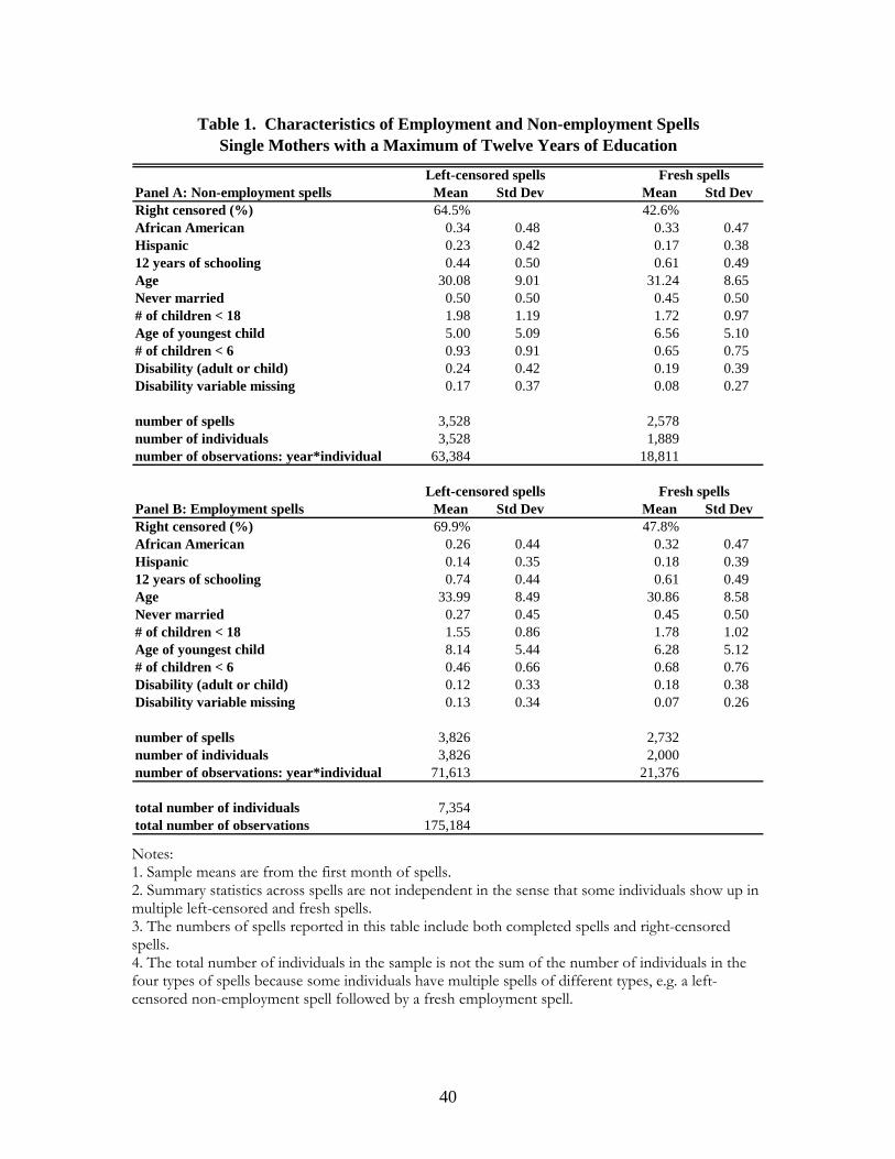
40

Panel A: Non-employment spells Mean Std Dev Mean Std DevRight censored (%) 64.5% 42.6%African American 0.34 0.48 0.33 0.47Hispanic 0.23 0.42 0.17 0.3812 years of schooling 0.44 0.50 0.61 0.49Age 30.08 9.01 31.24 8.65Never married 0.50 0.50 0.45 0.50# of children < 18 1.98 1.19 1.72 0.97Age of youngest child 5.00 5.09 6.56 5.10# of children < 6 0.93 0.91 0.65 0.75Disability (adult or child) 0.24 0.42 0.19 0.39Disability variable missing 0.17 0.37 0.08 0.27

number of spells 3,528 2,578number of individuals 3,528 1,889number of observations: year*individual 63,384 18,811

Panel B: Employment spells Mean Std Dev Mean Std DevRight censored (%) 69.9% 47.8%African American 0.26 0.44 0.32 0.47Hispanic 0.14 0.35 0.18 0.3912 years of schooling 0.74 0.44 0.61 0.49Age 33.99 8.49 30.86 8.58Never married 0.27 0.45 0.45 0.50# of children < 18 1.55 0.86 1.78 1.02Age of youngest child 8.14 5.44 6.28 5.12# of children < 6 0.46 0.66 0.68 0.76Disability (adult or child) 0.12 0.33 0.18 0.38Disability variable missing 0.13 0.34 0.07 0.26

number of spells 3,826 2,732number of individuals 3,826 2,000number of observations: year*individual 71,613 21,376

total number of individuals 7,354total number of observations 175,184

Table 1. Characteristics of Employment and Non-employment Spells Single Mothers with a Maximum of Twelve Years of Education

Left-censored spells Fresh spells

Left-censored spells Fresh spells

Notes: 1. Sample means are from the first month of spells. 2. Summary statistics across spells are not independent in the sense that some individuals show up in multiple left-censored and fresh spells. 3. The numbers of spells reported in this table include both completed spells and right-censored spells. 4. The total number of individuals in the sample is not the sum of the number of individuals in the four types of spells because some individuals have multiple spells of different types, e.g. a left-censored non-employment spell followed by a fresh employment spell.

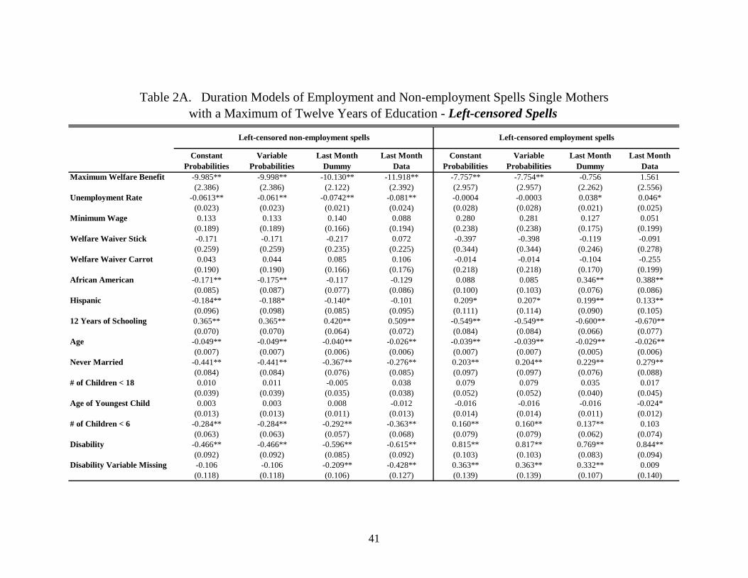
41

Constant Probabilities

Variable Probabilities

Last Month Dummy

Last Month Data

Constant Probabilities

Variable Probabilities

Last Month Dummy

Last Month Data

Maximum Welfare Benefit -9.985** -9.998** -10.130** -11.918** -7.757** -7.754** -0.756 1.561 (2.386) (2.386) (2.122) (2.392) (2.957) (2.957) (2.262) (2.556)Unemployment Rate -0.0613** -0.061** -0.0742** -0.081** -0.0004 -0.0003 0.038* 0.046* (0.023) (0.023) (0.021) (0.024) (0.028) (0.028) (0.021) (0.025)Minimum Wage 0.133 0.133 0.140 0.088 0.280 0.281 0.127 0.051 (0.189) (0.189) (0.166) (0.194) (0.238) (0.238) (0.175) (0.199)Welfare Waiver Stick -0.171 -0.171 -0.217 0.072 -0.397 -0.398 -0.119 -0.091 (0.259) (0.259) (0.235) (0.225) (0.344) (0.344) (0.246) (0.278)Welfare Waiver Carrot 0.043 0.044 0.085 0.106 -0.014 -0.014 -0.104 -0.255 (0.190) (0.190) (0.166) (0.176) (0.218) (0.218) (0.170) (0.199)African American -0.171** -0.175** -0.117 -0.129 0.088 0.085 0.346** 0.388** (0.085) (0.087) (0.077) (0.086) (0.100) (0.103) (0.076) (0.086)Hispanic -0.184** -0.188* -0.140* -0.101 0.209* 0.207* 0.199** 0.133** (0.096) (0.098) (0.085) (0.095) (0.111) (0.114) (0.090) (0.105)12 Years of Schooling 0.365** 0.365** 0.420** 0.509** -0.549** -0.549** -0.600** -0.670** (0.070) (0.070) (0.064) (0.072) (0.084) (0.084) (0.066) (0.077)Age -0.049** -0.049** -0.040** -0.026** -0.039** -0.039** -0.029** -0.026** (0.007) (0.007) (0.006) (0.006) (0.007) (0.007) (0.005) (0.006)Never Married -0.441** -0.441** -0.367** -0.276** 0.203** 0.204** 0.229** 0.279** (0.084) (0.084) (0.076) (0.085) (0.097) (0.097) (0.076) (0.088)# of Children < 18 0.010 0.011 -0.005 0.038 0.079 0.079 0.035 0.017 (0.039) (0.039) (0.035) (0.038) (0.052) (0.052) (0.040) (0.045)Age of Youngest Child 0.003 0.003 0.008 -0.012 -0.016 -0.016 -0.016 -0.024* (0.013) (0.013) (0.011) (0.013) (0.014) (0.014) (0.011) (0.012)# of Children < 6 -0.284** -0.284** -0.292** -0.363** 0.160** 0.160** 0.137** 0.103 (0.063) (0.063) (0.057) (0.068) (0.079) (0.079) (0.062) (0.074)Disability -0.466** -0.466** -0.596** -0.615** 0.815** 0.817** 0.769** 0.844**

(0.092) (0.092) (0.085) (0.092) (0.103) (0.103) (0.083) (0.094)Disability Variable Missing -0.106 -0.106 -0.209** -0.428** 0.363** 0.363** 0.332** 0.009

(0.118) (0.118) (0.106) (0.127) (0.139) (0.139) (0.107) (0.140)

Table 2A. Duration Models of Employment and Non-employment Spells Single Mothers with a Maximum of Twelve Years of Education - Left-censored Spells

Left-censored non-employment spells Left-censored employment spells

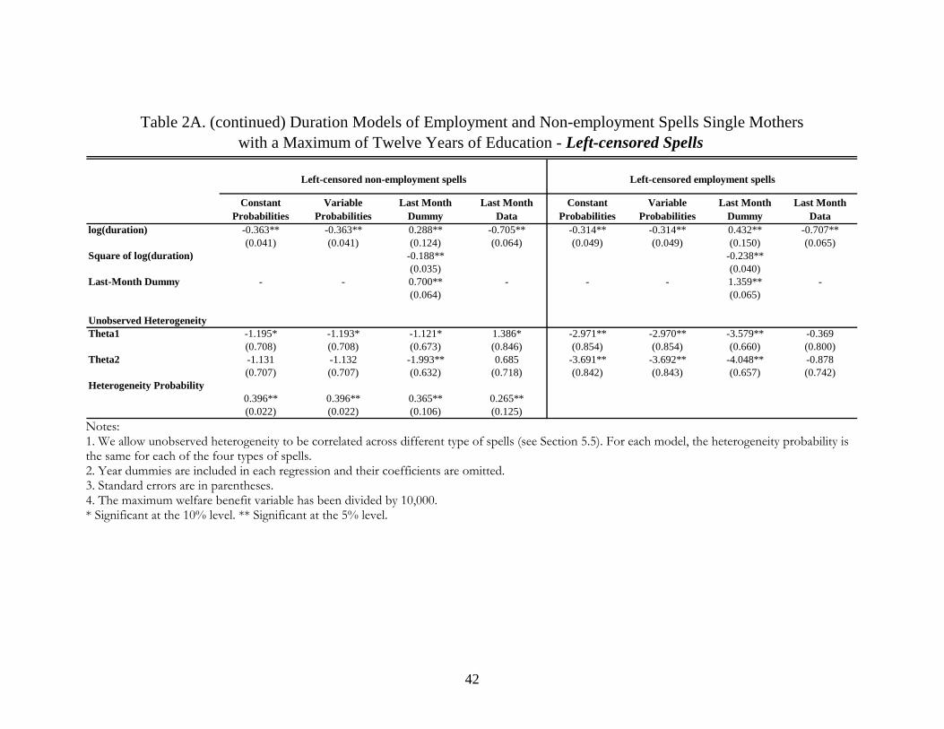
42

Constant Probabilities

Variable Probabilities

Last Month Dummy

Last Month Data

Constant Probabilities

Variable Probabilities

Last Month Dummy

Last Month Data

log(duration) -0.363** -0.363** 0.288** -0.705** -0.314** -0.314** 0.432** -0.707**(0.041) (0.041) (0.124) (0.064) (0.049) (0.049) (0.150) (0.065)

Square of log(duration) -0.188** -0.238**(0.035) (0.040)

Last-Month Dummy - - 0.700** - - - 1.359** -(0.064) (0.065)

Unobserved HeterogeneityTheta1 -1.195* -1.193* -1.121* 1.386* -2.971** -2.970** -3.579** -0.369 (0.708) (0.708) (0.673) (0.846) (0.854) (0.854) (0.660) (0.800)Theta2 -1.131 -1.132 -1.993** 0.685 -3.691** -3.692** -4.048** -0.878 (0.707) (0.707) (0.632) (0.718) (0.842) (0.843) (0.657) (0.742)Heterogeneity Probability

0.396** 0.396** 0.365** 0.265**(0.022) (0.022) (0.106) (0.125)

Left-censored non-employment spells Left-censored employment spells

Table 2A. (continued) Duration Models of Employment and Non-employment Spells Single Mothers with a Maximum of Twelve Years of Education - Left-censored Spells

Notes: 1. We allow unobserved heterogeneity to be correlated across different type of spells (see Section 5.5). For each model, the heterogeneity probability is the same for each of the four types of spells. 2. Year dummies are included in each regression and their coefficients are omitted. 3. Standard errors are in parentheses. 4. The maximum welfare benefit variable has been divided by 10,000. * Significant at the 10% level. ** Significant at the 5% level.

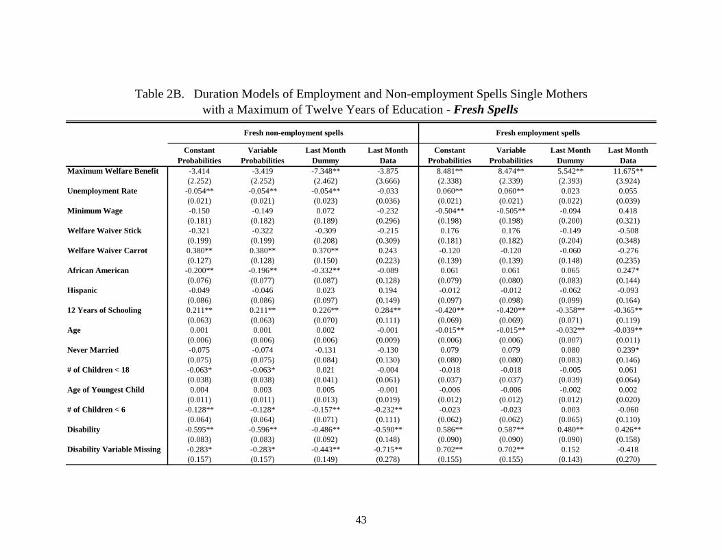
43

Constant Probabilities

Variable Probabilities

Last Month Dummy

Last Month Data

Constant Probabilities

Variable Probabilities

Last Month Dummy

Last Month Data

Maximum Welfare Benefit -3.414 -3.419 -7.348** -3.875 8.481** 8.474** 5.542** 11.675** (2.252) (2.252) (2.462) (3.666) (2.338) (2.339) (2.393) (3.924)Unemployment Rate -0.054** -0.054** -0.054** -0.033 0.060** 0.060** 0.023 0.055 (0.021) (0.021) (0.023) (0.036) (0.021) (0.021) (0.022) (0.039)Minimum Wage -0.150 -0.149 0.072 -0.232 -0.504** -0.505** -0.094 0.418 (0.181) (0.182) (0.189) (0.296) (0.198) (0.198) (0.200) (0.321)Welfare Waiver Stick -0.321 -0.322 -0.309 -0.215 0.176 0.176 -0.149 -0.508 (0.199) (0.199) (0.208) (0.309) (0.181) (0.182) (0.204) (0.348)Welfare Waiver Carrot 0.380** 0.380** 0.370** 0.243 -0.120 -0.120 -0.060 -0.276 (0.127) (0.128) (0.150) (0.223) (0.139) (0.139) (0.148) (0.235)African American -0.200** -0.196** -0.332** -0.089 0.061 0.061 0.065 0.247* (0.076) (0.077) (0.087) (0.128) (0.079) (0.080) (0.083) (0.144)Hispanic -0.049 -0.046 0.023 0.194 -0.012 -0.012 -0.062 -0.093 (0.086) (0.086) (0.097) (0.149) (0.097) (0.098) (0.099) (0.164)12 Years of Schooling 0.211** 0.211** 0.226** 0.284** -0.420** -0.420** -0.358** -0.365** (0.063) (0.063) (0.070) (0.111) (0.069) (0.069) (0.071) (0.119)Age 0.001 0.001 0.002 -0.001 -0.015** -0.015** -0.032** -0.039** (0.006) (0.006) (0.006) (0.009) (0.006) (0.006) (0.007) (0.011)Never Married -0.075 -0.074 -0.131 -0.130 0.079 0.079 0.080 0.239* (0.075) (0.075) (0.084) (0.130) (0.080) (0.080) (0.083) (0.146)# of Children < 18 -0.063* -0.063* 0.021 -0.004 -0.018 -0.018 -0.005 0.061 (0.038) (0.038) (0.041) (0.061) (0.037) (0.037) (0.039) (0.064)Age of Youngest Child 0.004 0.003 0.005 -0.001 -0.006 -0.006 -0.002 0.002 (0.011) (0.011) (0.013) (0.019) (0.012) (0.012) (0.012) (0.020)# of Children < 6 -0.128** -0.128* -0.157** -0.232** -0.023 -0.023 0.003 -0.060 (0.064) (0.064) (0.071) (0.111) (0.062) (0.062) (0.065) (0.110)Disability -0.595** -0.596** -0.486** -0.590** 0.586** 0.587** 0.480** 0.426**

(0.083) (0.083) (0.092) (0.148) (0.090) (0.090) (0.090) (0.158)Disability Variable Missing -0.283* -0.283* -0.443** -0.715** 0.702** 0.702** 0.152 -0.418

(0.157) (0.157) (0.149) (0.278) (0.155) (0.155) (0.143) (0.270)

Table 2B. Duration Models of Employment and Non-employment Spells Single Mothers with a Maximum of Twelve Years of Education - Fresh Spells

Fresh non-employment spells Fresh employment spells

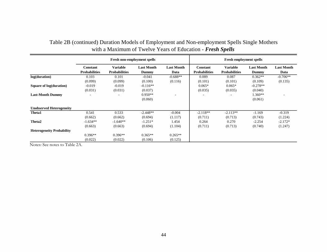
44

Constant Probabilities

Variable Probabilities

Last Month Dummy

Last Month Data

Constant Probabilities

Variable Probabilities

Last Month Dummy

Last Month Data

log(duration) 0.103 0.101 -0.041 -0.688** 0.089 0.087 0.362** -0.706**(0.099) (0.099) (0.100) (0.116) (0.101) (0.101) (0.109) (0.135)

Square of log(duration) -0.019 -0.019 -0.116** 0.065* 0.065* -0.278**(0.031) (0.031) (0.037) (0.035) (0.035) (0.040)

Last-Month Dummy - - 0.950** - - - 1.360** -(0.060) (0.061)

Unobserved HeterogeneityTheta1 0.541 0.533 -2.448** -0.004 -2.118** -2.113** -1.169 -0.319 (0.662) (0.662) (0.694) (1.117) (0.711) (0.713) (0.743) (1.224)Theta2 -1.634** -1.640** -1.251* 1.454 0.264 0.270 -2.254 -2.172* (0.663) (0.663) (0.694) (1.104) (0.711) (0.713) (0.740) (1.247)Heterogeneity Probability

0.396** 0.396** 0.365** 0.265**(0.022) (0.022) (0.106) (0.125)

Fresh non-employment spells Fresh employment spells

Table 2B (continued) Duration Models of Employment and Non-employment Spells Single Mothers with a Maximum of Twelve Years of Education - Fresh Spells

Notes: See notes to Table 2A.

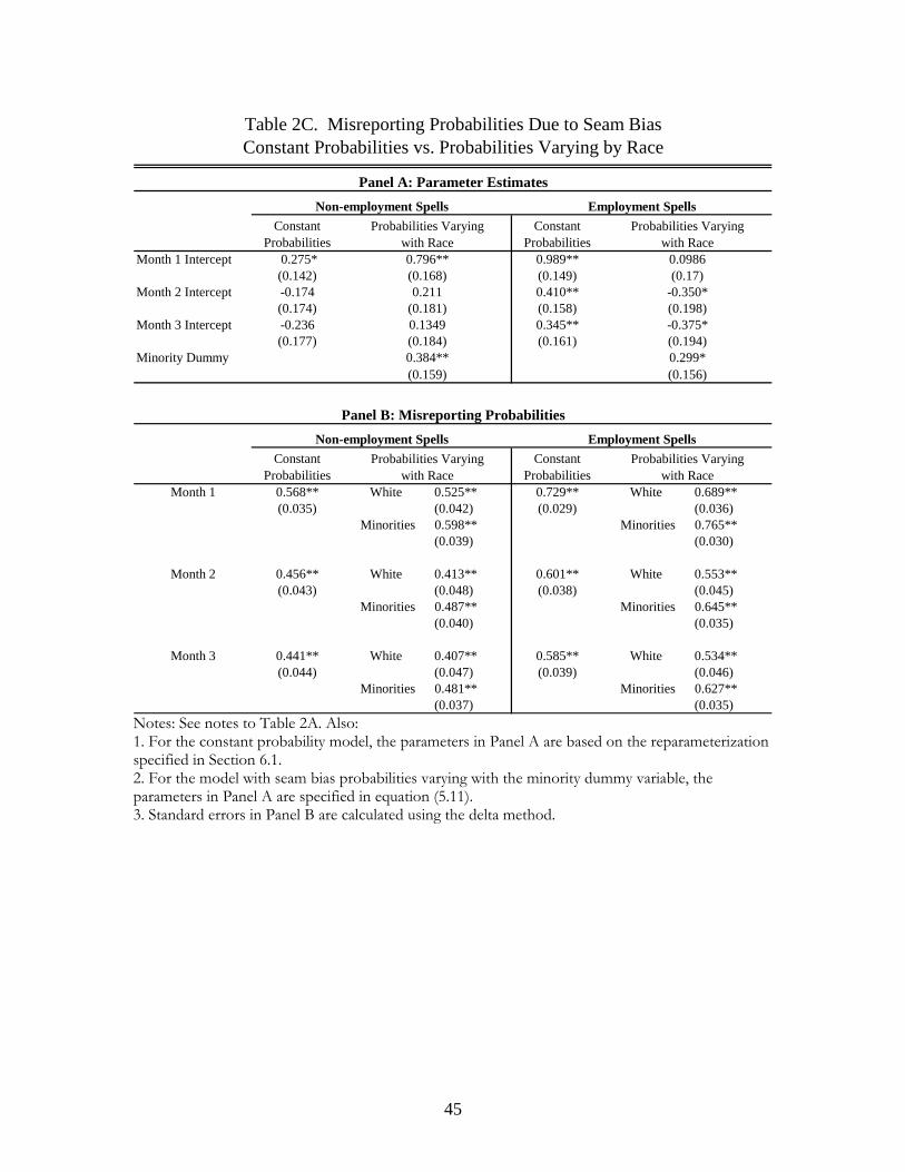
45

Constant Probabilities

Constant Probabilities

Month 1 Intercept 0.275* 0.989**(0.142) (0.149)

Month 2 Intercept -0.174 0.410**(0.174) (0.158)

Month 3 Intercept -0.236 0.345**(0.177) (0.161)

Minority Dummy

Constant Probabilities

Constant Probabilities

Month 1 0.568** White 0.525** 0.729** White 0.689**(0.035) (0.042) (0.029) (0.036)

Minorities 0.598** Minorities 0.765**(0.039) (0.030)

Month 2 0.456** White 0.413** 0.601** White 0.553**(0.043) (0.048) (0.038) (0.045)

Minorities 0.487** Minorities 0.645**(0.040) (0.035)

Month 3 0.441** White 0.407** 0.585** White 0.534**(0.044) (0.047) (0.039) (0.046)

Minorities 0.481** Minorities 0.627**(0.037) (0.035)

0.384**

Non-employment Spells Employment Spells

0.211(0.181)0.1349(0.184)

Probabilities Varying with Race

Probabilities Varying with Race

Table 2C. Misreporting Probabilities Due to Seam Bias Constant Probabilities vs. Probabilities Varying by Race

Panel A: Parameter Estimates

Probabilities Varying with Race0.796**

Panel B: Misreporting Probabilities

Non-employment Spells Employment Spells

(0.168)

(0.159)

Probabilities Varying with Race

0.0986(0.17)

-0.350*(0.198)-0.375*(0.194)0.299*(0.156)

Notes: See notes to Table 2A. Also: 1. For the constant probability model, the parameters in Panel A are based on the reparameterization specified in Section 6.1. 2. For the model with seam bias probabilities varying with the minority dummy variable, the parameters in Panel A are specified in equation (5.11). 3. Standard errors in Panel B are calculated using the delta method.

46

Note: See notes to Table 2A. Standard errors are calculated using the delta method.

Constant Misreporting Probabilities

Variable Misreporting Probabilities

Last-Month Dummy Model

Last Month Data

Constant Misreporting Probabilities

Variable Misreporting Probabilities

Last-Month Dummy Model

Last Month Data

39.305** 39.299** 35.478** 38.834** 42.248** 42.252** 38.999** 41.157**(0.731) (0.725) (0.574) (0.600) (0.608) (0.634) (0.533) (0.601)

0.515** 0.516** 0.552** 0.585 0.352 0.352 0.040 -0.074(0.143) (0.169) (0.185) (0.495) (0.359) (0.259) (0.112) (0.228)

-0.639 -0.654 -1.313 -1.498 0.168 0.165 1.436 3.055(2.892) (2.827) (2.608) (2.497) (2.655) (2.537) (2.253) (2.225)

2.427 2.427 3.228 -1.005 4.483 4.485 1.639 1.125(3.458) (3.503) (3.416) (3.195) (3.514) (3.537) (3.400) (3.374)

-0.768 -0.773 -0.841 -0.485 -1.381 -1.383 -0.707 -0.250(1.423) (1.079) (1.142) (1.345) (1.043) (1.201) (0.972) (0.873)

1.446** 1.445** 1.834** 1.806** 0.007 0.006 -0.898 -0.980(0.580) (0.713) (0.643) (0.599) (0.548) (0.587) (0.525) (0.628)

Constant Misreporting Probabilities

Variable Misreporting Probabilities

Last-Month Dummy Model

Last Month Data

Constant Misreporting Probabilities

Variable Misreporting Probabilities

Last-Month Dummy Model

Last Month Data

11.821** 11.827** 16.458** 23.342** 11.929** 11.920** 27.711** 32.563**(0.516) (0.514) (1.312) (2.254) (0.495) (0.497) (1.394) (2.197)

0.118 0.119 0.375** 0.196 -0.220** -0.220** -0.341* -0.565(0.119) (0.149) (0.136) (0.407) (0.070) (0.062) (0.206) (0.446)

-3.099** -3.103** -4.531** -3.139 0.881 0.885 0.988 3.471(1.009) (0.933) (1.703) (2.790) (1.074) (1.014) (2.471) (2.826)

3.138 3.152 4.388 2.950 -1.222 -1.220 2.453 6.266(2.100) (2.075) (3.212) (4.323) (1.217) (1.228) (3.355) (4.187)

0.545 0.540 -0.375 1.238 1.484** 1.486** 0.608 -2.133(0.613) (0.715) (1.027) (1.420) (0.538) (0.570) (1.180) (1.499)

0.835** 0.837** 1.226** 0.732 -0.693** -0.695** -0.633 -1.193(0.343) (0.354) (0.550) (0.892) (0.277) (0.249) (0.593) (0.826)

Table 3A. Expected Durations and the Effects of Changes in Macro and Public Policy Variables Employment and Non-employment Spells

Left-censored non-employment spells Left-censored employment spells

Average Expected Duration (in months)

Fresh employment spells

Average Expected Duration (in months)

Changes with respect to:

Maximum welfare benefits increasing by 10%

Minimum wage increasing by 10%

Unemployment rate increasing by 25%

Stick waiver (implemented - not implemented)

Carrot waiver (implemented - not implemented)

Fresh non-employment spells

Unemployment rate increasing by 25%

Changes with respect to:

Maximum welfare benefits increasing by 10%

Carrot waiver (implemented - not implemented)

Stick waiver (implemented - not implemented)

Minimum wage increasing by 10%

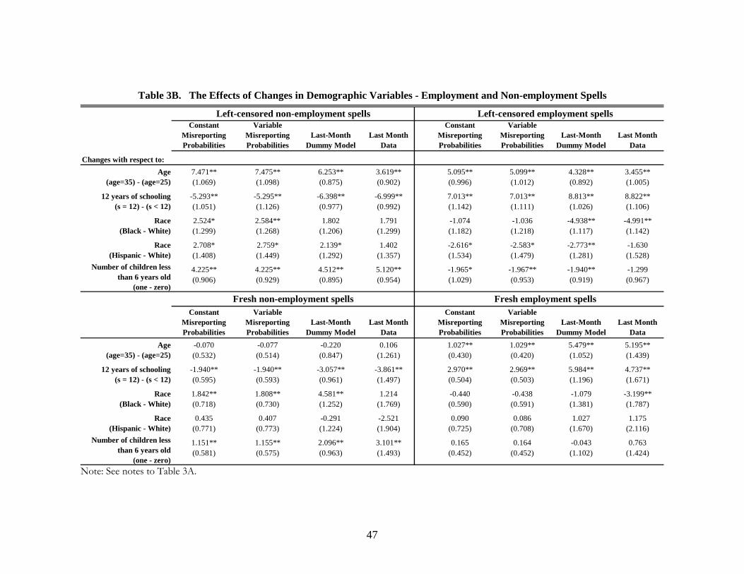
47

Note: See notes to Table 3A.

Constant Misreporting Probabilities

Variable Misreporting Probabilities

Last-Month Dummy Model

Last Month Data

Constant Misreporting Probabilities

Variable Misreporting Probabilities

Last-Month Dummy Model

Last Month Data

7.471** 7.475** 6.253** 3.619** 5.095** 5.099** 4.328** 3.455**(1.069) (1.098) (0.875) (0.902) (0.996) (1.012) (0.892) (1.005)

-5.293** -5.295** -6.398** -6.999** 7.013** 7.013** 8.813** 8.822**(1.051) (1.126) (0.977) (0.992) (1.142) (1.111) (1.026) (1.106)

2.524* 2.584** 1.802 1.791 -1.074 -1.036 -4.938** -4.991**(1.299) (1.268) (1.206) (1.299) (1.182) (1.218) (1.117) (1.142)

2.708* 2.759* 2.139* 1.402 -2.616* -2.583* -2.773** -1.630(1.408) (1.449) (1.292) (1.357) (1.534) (1.479) (1.281) (1.528)

4.225** 4.225** 4.512** 5.120** -1.965* -1.967** -1.940** -1.299(0.906) (0.929) (0.895) (0.954) (1.029) (0.953) (0.919) (0.967)

Constant Misreporting Probabilities

Variable Misreporting Probabilities

Last-Month Dummy Model

Last Month Data

Constant Misreporting Probabilities

Variable Misreporting Probabilities

Last-Month Dummy Model

Last Month Data

-0.070 -0.077 -0.220 0.106 1.027** 1.029** 5.479** 5.195**(0.532) (0.514) (0.847) (1.261) (0.430) (0.420) (1.052) (1.439)

-1.940** -1.940** -3.057** -3.861** 2.970** 2.969** 5.984** 4.737**(0.595) (0.593) (0.961) (1.497) (0.504) (0.503) (1.196) (1.671)

1.842** 1.808** 4.581** 1.214 -0.440 -0.438 -1.079 -3.199**(0.718) (0.730) (1.252) (1.769) (0.590) (0.591) (1.381) (1.787)

0.435 0.407 -0.291 -2.521 0.090 0.086 1.027 1.175(0.771) (0.773) (1.224) (1.904) (0.725) (0.708) (1.670) (2.116)

1.151** 1.155** 2.096** 3.101** 0.165 0.164 -0.043 0.763(0.581) (0.575) (0.963) (1.493) (0.452) (0.452) (1.102) (1.424)

Table 3B. The Effects of Changes in Demographic Variables - Employment and Non-employment Spells

Left-censored non-employment spells Left-censored employment spells

Fresh employment spells

Age (age=35) - (age=25)

12 years of schooling (s = 12) - (s < 12)

Race (Black - White)

Race (Hispanic - White)

Number of children less than 6 years old

(one - zero)

Fresh non-employment spells

Race (Hispanic - White)

Number of children less than 6 years old

(one - zero)

Age (age=35) - (age=25)

12 years of schooling (s = 12) - (s < 12)

Race (Black - White)

Changes with respect to:

48

Constant Probabilities

Probabilities Varying with Race

Constant Probabilities

Probabilities Varying with Race

Seam Bias Parameters:Month 1 Intercept 0.814** 1.614** 1.822** 0.605**

(0.217) (0.389) (0.314) (0.264)Month 2 Intercept 0.257 0.837** 1.024** 0.041

(0.220) (0.321) (0.259) (0.270)Month 3 Intercept 0.083 0.592* 0.802** -0.089

(0.216) (0.314) (0.222) (0.254)Minority Dummy 0.3559 0.3499

(0.348) (0.253)

Fraction of individuals reporting accuratelyIntercept -1.694** -1.596**

(0.227) (0.365)Minority Dummy -0.224

(0.457)

Table 4. Misreporting Estimates for the Models Where a Fraction of the Population Never Misreports

Panel A: Parameter Estimates

Non-employment Spells Employment Spells

Constant Probabilities

Constant Probabilities

Month 1 0.693 White 0.647 0.861 White 0.834(0.046) (0.060) (0.038) (0.054)

Minorities 0.722 Minorities 0.878(0.048) (0.036)

Month 2 0.564 White 0.510 0.736 White 0.698(0.054) (0.067) (0.050) (0.068)

Minorities 0.597 Minorities 0.767(0.058) (0.055)

Month 3 0.521 White 0.478 0.690 White 0.644(0.054) (0.063) (0.047) (0.072)

Minorities 0.565 Minorities 0.721(0.062) (0.051)

0.155 White 0.169(0.030) (0.051)

Minorities 0.139(0.035)

Fraction of Accurate Reporting

Panel B: Misreporting ProbabilitiesNon-employment Spells Employment Spells

Probabilities Varying with Race

Probabilities Varying with Race

Notes: See notes to Table 2C.

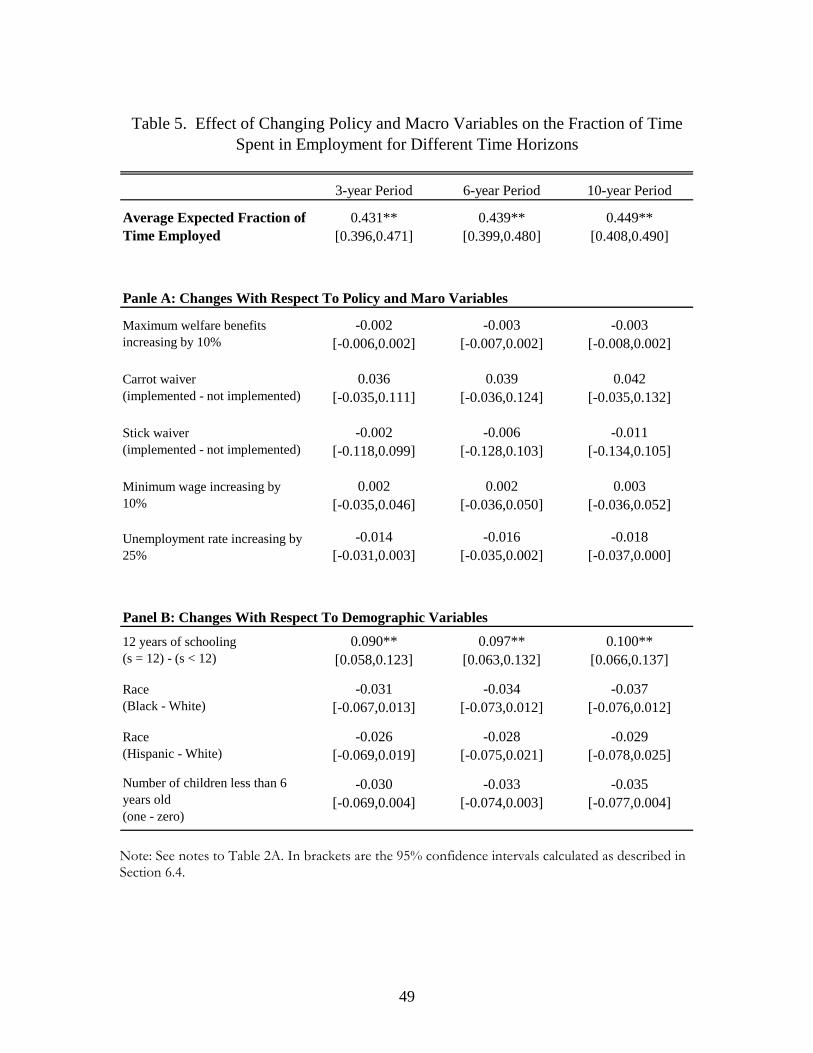
49

3-year Period 6-year Period 10-year Period

0.431** 0.439** 0.449**[0.396,0.471] [0.399,0.480] [0.408,0.490]

-0.002 -0.003 -0.003[-0.006,0.002] [-0.007,0.002] [-0.008,0.002]

0.036 0.039 0.042[-0.035,0.111] [-0.036,0.124] [-0.035,0.132]

-0.002 -0.006 -0.011[-0.118,0.099] [-0.128,0.103] [-0.134,0.105]

0.002 0.002 0.003[-0.035,0.046] [-0.036,0.050] [-0.036,0.052]

-0.014 -0.016 -0.018[-0.031,0.003] [-0.035,0.002] [-0.037,0.000]

0.090** 0.097** 0.100**[0.058,0.123] [0.063,0.132] [0.066,0.137]

-0.031 -0.034 -0.037[-0.067,0.013] [-0.073,0.012] [-0.076,0.012]

-0.026 -0.028 -0.029[-0.069,0.019] [-0.075,0.021] [-0.078,0.025]

-0.030 -0.033 -0.035[-0.069,0.004] [-0.074,0.003] [-0.077,0.004]

12 years of schooling (s = 12) - (s < 12)

Race (Black - White)

Race (Hispanic - White)

Number of children less than 6 years old (one - zero)

Table 5. Effect of Changing Policy and Macro Variables on the Fraction of Time Spent in Employment for Different Time Horizons

Average Expected Fraction of Time Employed

Panle A: Changes With Respect To Policy and Maro Variables

Maximum welfare benefits increasing by 10%

Carrot waiver (implemented - not implemented)

Stick waiver (implemented - not implemented)

Minimum wage increasing by 10%

Unemployment rate increasing by 25%

Panel B: Changes With Respect To Demographic Variables

Note: See notes to Table 2A. In brackets are the 95% confidence intervals calculated as described in Section 6.4.

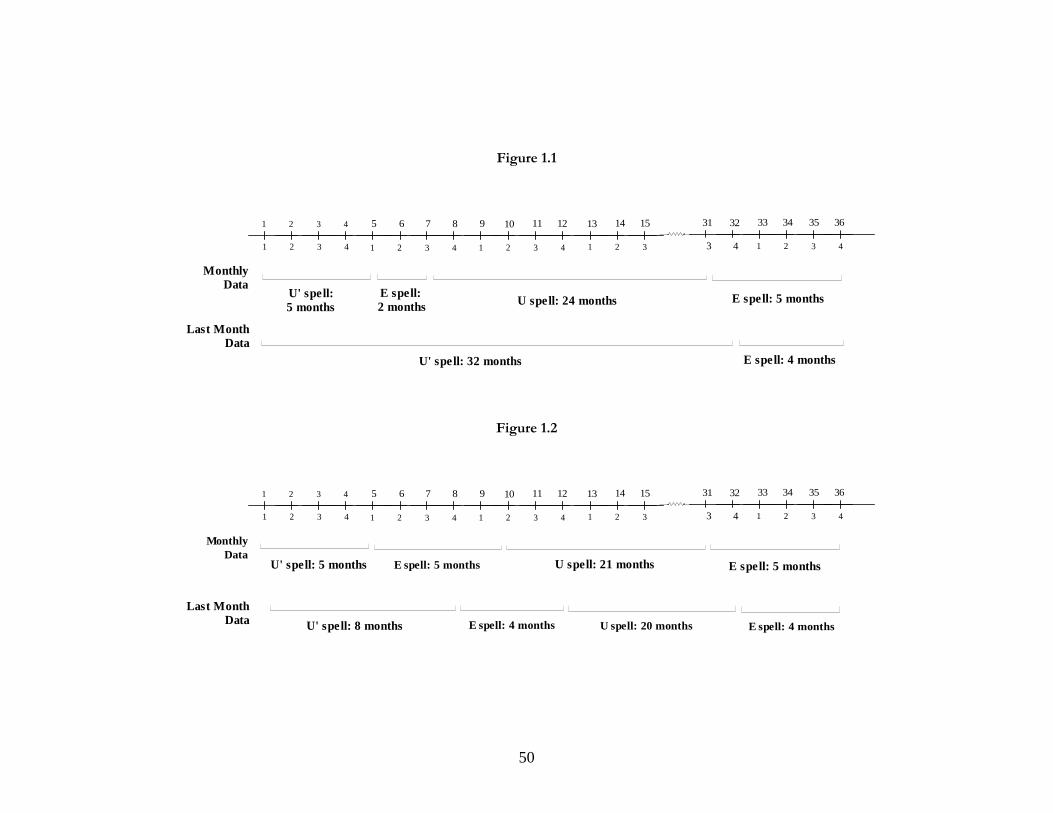
50

Figure 1.1

Figure 1.2

1 2 3 4 5 6 7 8

1 2 3 4 1 2 3 4

9 10 11 12

1 2 3 4

13 14 15 31 32 33 34

1 2 3 1 2 3 4

35 36

3 4

MonthlyData

Last MonthData E spell: 4 monthsU' spell: 8 months U spell: 20 months E spell: 4 months

E spell: 5 monthsU' spell: 5 months U spell: 21 months E spell: 5 months

1 2 3 4 5 6 7 8

1 2 3 4 1 2 3 4

9 10 11 12

1 2 3 4

13 14 15 31 32 33 34

1 2 3 1 2 3 4

35 36

3 4

E spell: 2 months

U' spell:5 months U spell: 24 months

MonthlyData

E spell: 5 months

U' spell: 32 months E spell: 4 months

Last MonthData

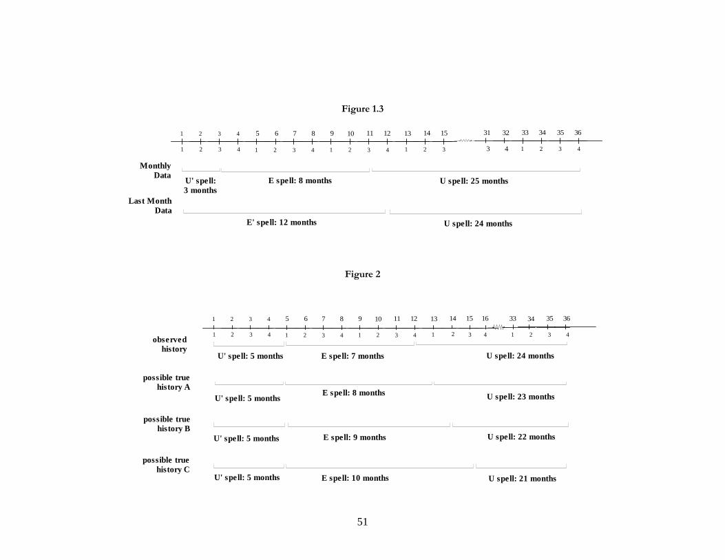
51

Figure 1.3

Figure 2

E spell: 7 monthsU' spell: 5 months U spell: 24 months

observedhistory

U' spell: 5 months

U' spell: 5 months

U' spell: 5 months

E spell: 8 months

E spell: 9 months

E spell: 10 months

U spell: 23 months

U spell: 22 months

U spell: 21 months

possible truehistory A

possible truehistory B

possible truehistory C

1 2 3 4 5 6 7 8

1 2 3 4 1 2 3 4

9 10 11 12

1 2 3 4

13 14 15 33 34 35 36

1 2 3 1 2 3 4

16

4

1 2 3 4 5 6 7 8

1 2 3 4 1 2 3 4

9 10 11 12

1 2 3 4

13 14 15 31 32 33 34

1 2 3 1 2 3 4

35 36

3 4

MonthlyData

E' spell: 12 months U spell: 24 months

E spell: 8 months U spell: 25 months

Last MonthData

U' spell:3 months

52

Appendix 1: Derivations of the Contribution to the Likelihood Function for a Completed Spell of Observed Length K Ending in Months 1, 2, 3, or 4 of Reference Period l

Given assumptions A1 through A5 in Section 5, the contribution to the likelihood function

for a completed spell of observed length K that ends in months 1, 2, 3, or 4 of reference period l is:

1, ,

1, , 1, , 1, , 1, , .

obs obs

obs true true obs true true

P M l dur K

P M l M l dur K P M l M l dur K

Since the second term is zero by assumption A2, we have

1

1, , 1, , 1, ,

1, | 1, , 1,

1 ( ),

obs obs obs true true

obs true true true true true

P M l dur K P M l M l dur K

P M l M l dur K P M l dur K P dur K

L K

In the above derivation, we have used the implication of assumption A3 that

11, | 1, , 1 .obs true trueP M l M l dur K

Moreover,

1, 1true trueP M l dur K and ( ).trueP dur K L K

Similarly, if a transition is reported to end in month 2 or month 3 of reference period l , and to have

lasted for K months, we have

22, , 1obs obsP M l dur K L K and

33, , = (1 ) .obs obsP M l dur K L K

Finally, the contribution to the likelihood function of a completed spell of observed length K that is

observed to end in month 4 of reference period l is given by

4, ,

4, , 1, 1 , 1 4, , 2, 1 , 2

4, , 3, 1 , 3 4, , 4, ,

4, | 1, 1 , 1 1, 1

obs obs

obs true true obs true true

obs true true obs true true

obs true true true

P M l dur K

P M l M l dur K P M l M l dur K

P M l M l dur K P M l M l dur K

P M l M l dur K P M l dur

1 1

4, | 2, 1 , 2 2, 1 2 2

4, | 3, 1 , 3 3, 1 3 3

4, | 4, , 4,

true true

obs true true true true true

obs true true true true true

obs true true true

K P dur K

M l M l dur K P M l dur K P dur K

M l M l dur K P M l dur K P dur K

M l M l dur K P M

.true truel dur K P dur K

Note that 4, | 4, , 1obs true trueP M l M l dur K by assumption A4, and

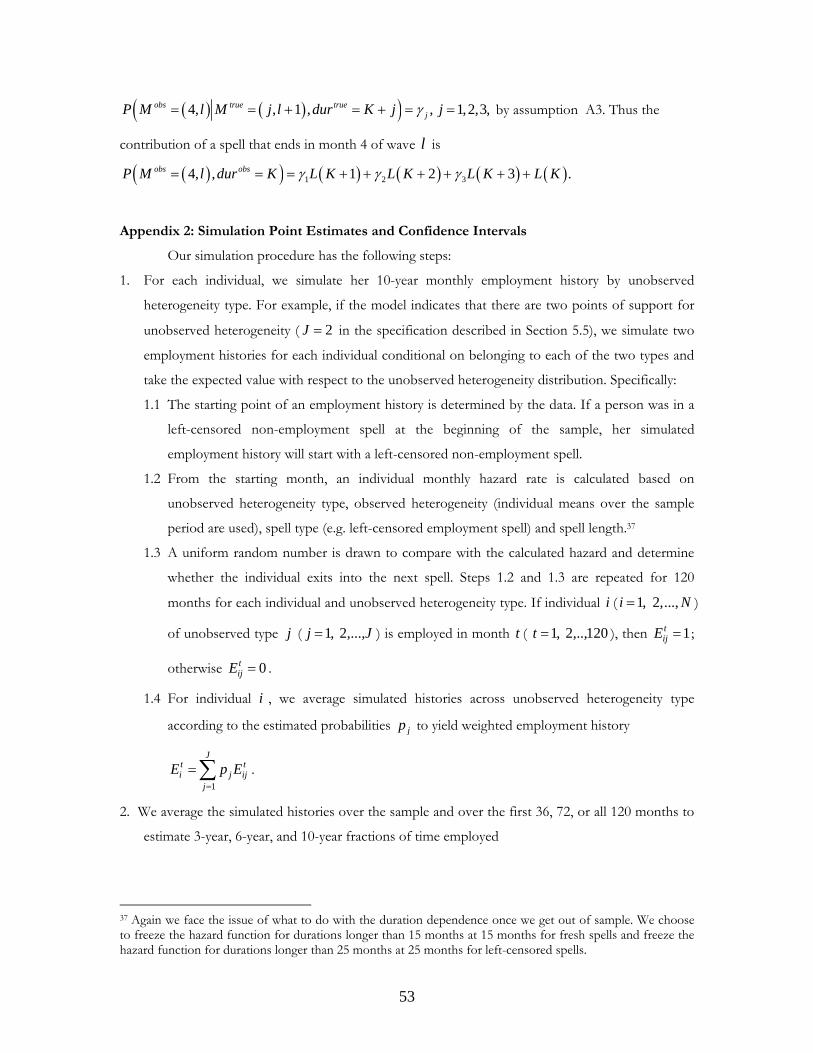
53

4, , 1 , , 1,2,3,obs true truejP M l M j l dur K j j by assumption A3. Thus the

contribution of a spell that ends in month 4 of wave l is

1 2 34, , 1 2 3 .obs obsP M l dur K L K L K L K L K

Appendix 2: Simulation Point Estimates and Confidence Intervals

Our simulation procedure has the following steps:

1. For each individual, we simulate her 10-year monthly employment history by unobserved

heterogeneity type. For example, if the model indicates that there are two points of support for

unobserved heterogeneity ( 2J in the specification described in Section 5.5), we simulate two

employment histories for each individual conditional on belonging to each of the two types and

take the expected value with respect to the unobserved heterogeneity distribution. Specifically:

1.1 The starting point of an employment history is determined by the data. If a person was in a

left-censored non-employment spell at the beginning of the sample, her simulated

employment history will start with a left-censored non-employment spell.

1.2 From the starting month, an individual monthly hazard rate is calculated based on

unobserved heterogeneity type, observed heterogeneity (individual means over the sample

period are used), spell type (e.g. left-censored employment spell) and spell length.37

1.3 A uniform random number is drawn to compare with the calculated hazard and determine

whether the individual exits into the next spell. Steps 1.2 and 1.3 are repeated for 120

months for each individual and unobserved heterogeneity type. If individual i ( 1, 2,...,i N )

of unobserved type j ( 1, 2,...,j J ) is employed in month t ( 1, 2,..,120t ), then 1tijE ;

otherwise 0tijE .

1.4 For individual i , we average simulated histories across unobserved heterogeneity type

according to the estimated probabilities jp to yield weighted employment history

1

Jt ti j ij

j

E p E

.

2. We average the simulated histories over the sample and over the first 36, 72, or all 120 months to

estimate 3-year, 6-year, and 10-year fractions of time employed

37 Again we face the issue of what to do with the duration dependence once we get out of sample. We choose to freeze the hazard function for durations longer than 15 months at 15 months for fresh spells and freeze the hazard function for durations longer than 25 months at 25 months for left-censored spells.

54

36

1 13 36

Nti

i tyr

EER

N

72

1 16 72

Nti

i tyr

EER

N

120

1 110 120

Nti

i tyr

EER

N

3. We use the CI-bootstrap to calculate the 95% confidence interval for the fraction of time

employed estimates as follows:

3.1 We generate 20,000 parameter vectors from the estimated asymptotic distribution.

3.2 We keep the parameter vectors that are within the 95% confidence interval of the parameter

estimates.

3.3 We calculate 3yrER , 6 yrER and 10 yrER for each parameter vector from step 3.2.

3.4 We take the minimum and maximum of 3yrER , 6 yrER and 10 yrER estimates from step 3.3,

respectively, and report them as the lower bound and upper bound of the estimated 95%

confidence interval for 3yrER , 6 yrER and 10 yrER .

4. To predict the effect of changing one variable on the above three fractions, we follow the

previous steps by setting the variable of interest at different levels for each person and then

taking the difference in estimated fractions. For example, to estimate the effect of implementing

positive incentives to leave welfare (“carrot” waiver policy), we first set the carrot waiver dummy

to 1 for each person (i.e. carrot waivers are implemented in all states) to calculate 13yrER , 1

6 yrER

and 110 yrER , and then set the carrot waiver dummy to 0 for each person (i.e. carrot waivers are

not implemented in any state) to calculate 03yrER , 0

6 yrER and 010 yrER . The terms 1 0

3 3yr yrER ER ,

1 06 6yr yrER ER and 1 0

10 10yr yrER ER are the estimated effects of implementing a positive incentive

to leave welfare.

5. We estimate 95% confidence intervals for the effects of changing variables following step 3 at

each level of those variables.

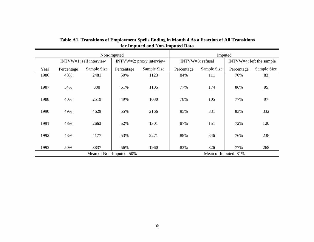
55

Year Percentage Sample Size Percentage Sample Size Percentage Sample Size Percentage Sample Size

1986 48% 2481 50% 1123 84% 111 70% 83

1987 54% 308 51% 1105 77% 174 86% 95

1988 40% 2519 49% 1030 78% 105 77% 97

1990 49% 4629 55% 2166 85% 331 83% 332

1991 48% 2663 52% 1301 87% 151 72% 120

1992 48% 4177 53% 2271 88% 346 76% 238

1993 50% 3837 56% 1960 83% 326 77% 268

Table A1. Transitions of Employment Spells Ending in Month 4 As a Fraction of All Transitions for Imputed and Non-Imputed Data

Non-imputed ImputedINTVW=1: self interview INTVW=2: proxy interview INTVW=3: refusal INTVW=4: left the sample

Mean of Non-Imputed: 50% Mean of Imputed: 81%