Embed Size (px)
Citation preview
CER
N-T
HES
IS-2
013-
049
26/0
4/20
13
UNIVERSITY OF OXFORD
Searches for New Physics
using Dijet Angular Distributions in
proton-proton collisions at√s = 7 TeV
collected with the ATLAS Detector
by
Ryan Mark Buckinghamof
St Edmund Hall
Oxford
Thesis submitted in partial fulfilment of the requirements
for the degree of Doctor of Philosophy
Hilary Term, 2013
UNIVERSITY OF OXFORD
Abstract
Searches for New Physics using Dijet Angular Distributions in proton-proton
collisions at√s = 7 TeV collected with the ATLAS Detector
by Ryan Mark Buckingham
Angular distributions of jet pairs (dijets) produced in proton-proton collisions at a centre-of-
mass energy√s = 7 TeV have been studied with the ATLAS detector at the Large Hadron
Collider using the full 2011 data set with an integrated luminosity of 4.8 fb−1, and reaching
dijet masses up to 4.5 TeV. All angular distributions are consistent with QCD predictions.
Analysis of the dijet angular distribution, using a novel technique simultaneously employing
the dijet mass, is employed. This analysis is sensitive to both resonant new physics and
phenomena with a slow-onset in mass. Using this technique, new exclusion limits have been
set at 95% credibility level for several hypotheses of physics beyond the standard model
including: quantum gravity scales, with 6 extra dimensions, below 4.11 TeV, quark contact
interactions below a compositeness scale of 7.6 TeV, and excited quarks with a mass below
2.75 TeV.
In a large and complex scientific experiment, such as ATLAS, the collection, management
and usability of coherent data and metadata is a challenging operation. The availability
of these data to physicists within the experiment is essential to all analysis efforts. A new
web-based interface called “RunBrowser”, which makes ATLAS and LHC operations data
available to the ATLAS Collaboration, is introduced.
Acknowledgements
The journey from inquisitive young boy, to the completion of this thesis, has been aided by
many. Here I would like to offer special thanks to some of these.
I believe I have been extremely lucky throughout my schooling to be blessed with enthusiastic,
dedicated and knowledgable teachers. My first thanks must go Mrs. West at Lutterworth
Grammar School, who pushed me beyond the regular physics curriculum at an early stage.
This trend was matched, and furthered, by my experiences at Leicester Grammar School,
where thanks to Mr. Inchley, Mr. Cawston, Mr. Handford and especially Mrs. Price, I was
pushed to my maximum and given the confidence to strive to pursue a course in academia
to the highest standards.
My time at St Edmund Hall will no doubt be among the happiest of my life. I am indebted
to many of the college fellows for their guidance and advice throughout my time as JCR
President and other roles. Thank-you for an unforgettable 8 years.
As my tutors at St Edmund Hall, I must thank Philipp Podsiadlowski and Jeff Tseng for, yet
again, pushing me to strive to the highest targets and for offering essential advice throughout.
Thank-you both.
As a first year undergraduate, I was lucky enough to take part in a summer research project
with Muge Karagoz Yamaoka, Todd Huffman, Jeff Tseng and Farrukh Azfar. This experience
sowed the seeds for an enthusiasm for experimental particle physics which would ultimately
lead me to this thesis. Thank-you for this opportunity.
Thank-you to Elizabeth Gallas for a fantastic first year project, and ATLAS authorship task.
Not only did this project enable me to present my results at the CHEP 2010 conference in
Taiwan, it also helped me develop many skills that will be useful beyond physics.
Upon moving to CERN, I joined the Exotics Dijet Team. Here I must thank Frederik Ruehr,
Georgios Choudalakis, Nele Boelaert, Thorsten Dietzsch, Mike Shupe and Caterina Doglioni.
I had a fantastic time working in this team of brilliant people, and enjoyed learning lots from
everyone.
Within the Oxford ATLAS Group, I must also thank Alan Barr, Claire Gwenlan, Tony
Weidberg, Hugo Beauchemin and Chris Hayes for their help over the past 4 years. I am also
very thankful to my peers (over multiple years) for productive discussions over daily coffees
and Friday night beers: Alex Pinder, Dan Short, Sam Whitehead, Chris Boddy, Caterina
ii

iii
Doglioni (Queen of Jets), Sarah Livermore, Nick Ryder, Adrian Lewis, Ellie Davies, Chris
Young, Robert King, David Hall, Lucy Kogan and Alex Dafinca.
With regards to this thesis, I am, of course, most indebted to my supervisor: Cigdem Issever,
whose guidance, enthusiasm and management, stirred my curiosity and encouraged me to
dive straight into the ATLAS Collaboration: striving to contribute and gain responsibility
at an early stage. I believe this approach put me in good stead to publish meaningful results,
and to ultimately produce this work.
Finally, I would like to thank the STFC, St Edmund Hall, the Institute of Physics and the
University of Oxford Department of Physics for their financial support over the last 4 years.
Thank-you all.
Contents
Abstract i
Acknowledgements ii
List of Figures vii
List of Tables xi
1 Introduction 1
1.1 New physics searches . . . . . . . . . . . . . . . . . . . . . . . . . . . . . . . 2
1.2 An overview of the Standard Model . . . . . . . . . . . . . . . . . . . . . . . 3
1.3 Searches for New Physics using Dijet Angular Distributions in proton-protoncollisions at
√s = 7 TeV collected with the ATLAS Detector . . . . . . . . . 6
1.4 Author’s contribution . . . . . . . . . . . . . . . . . . . . . . . . . . . . . . . 8
2 Collider physics and quantum chromodynamics 11
2.1 Scattering experiments and the parton model . . . . . . . . . . . . . . . . . 12
2.2 Quantum chromodynamics . . . . . . . . . . . . . . . . . . . . . . . . . . . . 13
2.3 The cross-section for a hard hadronic process . . . . . . . . . . . . . . . . . . 19
2.4 Monte Carlo simulation of QCD processes . . . . . . . . . . . . . . . . . . . 21
2.5 QCD Monte Carlo simulation used in this thesis . . . . . . . . . . . . . . . . 23
3 Experimental apparatus 25
3.1 The Large Hadron Collider . . . . . . . . . . . . . . . . . . . . . . . . . . . . 25
3.2 Overview of the ATLAS detector . . . . . . . . . . . . . . . . . . . . . . . . 28
3.3 The ATLAS trigger system . . . . . . . . . . . . . . . . . . . . . . . . . . . . 36
3.4 Simulation of the ATLAS detector . . . . . . . . . . . . . . . . . . . . . . . . 37
3.5 Data used in this thesis . . . . . . . . . . . . . . . . . . . . . . . . . . . . . . 38
4 Beyond the standard model 40
4.1 Extra dimensions . . . . . . . . . . . . . . . . . . . . . . . . . . . . . . . . . 40
iv
Contents v
4.2 Quantum Black Holes . . . . . . . . . . . . . . . . . . . . . . . . . . . . . . . 46
4.3 Quark sub-structure . . . . . . . . . . . . . . . . . . . . . . . . . . . . . . . 49
5 Jet reconstruction 55
5.1 Motivations for jet definitions . . . . . . . . . . . . . . . . . . . . . . . . . . 55
5.2 Jet finding algorithms in ATLAS . . . . . . . . . . . . . . . . . . . . . . . . 56
5.3 Jet reconstruction in ATLAS . . . . . . . . . . . . . . . . . . . . . . . . . . . 58
5.4 Jet energy scale & calibration . . . . . . . . . . . . . . . . . . . . . . . . . . 59
5.5 Jet uncertainties . . . . . . . . . . . . . . . . . . . . . . . . . . . . . . . . . 62
6 Searches for new physics with dijet angular distributions 66
6.1 Leading order dijet production . . . . . . . . . . . . . . . . . . . . . . . . . . 66
6.2 Angular dependence of dijet cross-section . . . . . . . . . . . . . . . . . . . . 69
6.3 Maximising sensitivity to the partonic cross-section . . . . . . . . . . . . . . 73
6.4 Experimental observables for NP searches . . . . . . . . . . . . . . . . . . . 77
6.5 Definition of control regions . . . . . . . . . . . . . . . . . . . . . . . . . . . 82
7 Event selection, systematic uncertainties and resulting distributions 83
7.1 Event selection . . . . . . . . . . . . . . . . . . . . . . . . . . . . . . . . . . 83
7.2 Histogram binning and trigger strategy . . . . . . . . . . . . . . . . . . . . . 88
7.3 QCD predictions . . . . . . . . . . . . . . . . . . . . . . . . . . . . . . . . . 91
7.4 Theoretical systematic uncertainties . . . . . . . . . . . . . . . . . . . . . . . 93
7.5 Experimental systematic uncertainties . . . . . . . . . . . . . . . . . . . . . 96
7.6 Summary of systematics . . . . . . . . . . . . . . . . . . . . . . . . . . . . . 99
7.7 Studies of the effects of pileup . . . . . . . . . . . . . . . . . . . . . . . . . . 101
7.8 Effects from detector malfunction . . . . . . . . . . . . . . . . . . . . . . . . 103
7.9 Validation of the QCD background . . . . . . . . . . . . . . . . . . . . . . . 105
7.10 Final distributions . . . . . . . . . . . . . . . . . . . . . . . . . . . . . . . . 106
8 Statistical interpretation and limits on signals for new physics 112
8.1 Search phase: is there evidence of new physics? . . . . . . . . . . . . . . . . 113
8.2 Limit-setting phase: constraints on new physics . . . . . . . . . . . . . . . . 121
9 Summary and conclusions 130
9.1 Summary of results . . . . . . . . . . . . . . . . . . . . . . . . . . . . . . . . 130
9.2 Comparison of dijet analysis techniques . . . . . . . . . . . . . . . . . . . . . 133
9.3 Future work and conclusions . . . . . . . . . . . . . . . . . . . . . . . . . . . 135
10 Metadata aided run selection 136
10.1 Introduction & motivation . . . . . . . . . . . . . . . . . . . . . . . . . . . . 136
10.2 ATLAS Conditions Database . . . . . . . . . . . . . . . . . . . . . . . . . . 137
10.3 Event selection using ATLAS TAGS . . . . . . . . . . . . . . . . . . . . . . . 138
10.4 runBrowser - Dynamic metadata aided Run selection . . . . . . . . . . . . . 139
10.5 Conclusions and future work . . . . . . . . . . . . . . . . . . . . . . . . . . . 143
Contents vi
A Determination of binning in χ and mjj 145
A.1 Determination of binning in χ . . . . . . . . . . . . . . . . . . . . . . . . . . 145
A.2 Determination of fine binning in mjj . . . . . . . . . . . . . . . . . . . . . . 146
B Comparing ATLFAST II to Geant full simulation 148
C Determination of trigger efficiencies 150
D Debug stream investigation in early data 153
E BlackMax paramter.txt 155
F Pileup reweighting 160
G Cut flows for signal samples 162
Bibliography 164
List of Figures
2.1 Loop corrections to the gluon propagator. . . . . . . . . . . . . . . . . . . . 15
2.2 Parton kinematics in the x,Q2 plane for (a) Tevatron and (b) LHC colliders. 18
2.3 Proton PDF distributions for√s = 7 TeV as a function of x according to the
MSTW collaboration. . . . . . . . . . . . . . . . . . . . . . . . . . . . . . . . 19
2.4 Schematic for a proton-proton collision resulting in a hard-scatter betweentwo partons. Other possible interactions from initial and final state radiationand underlying event are also included. . . . . . . . . . . . . . . . . . . . . . 20
2.5 LO, NLO and NNLO cross-section for inclusive jet cross-section as a functionof leading jet pT . . . . . . . . . . . . . . . . . . . . . . . . . . . . . . . . . . 21
3.1 Underground layout of the LHC tunnel. . . . . . . . . . . . . . . . . . . . . . 26
3.2 Cross section for various processes as a function of centre of mass collisionenergy and the event rate. . . . . . . . . . . . . . . . . . . . . . . . . . . . . 27
3.3 The ATLAS detector. . . . . . . . . . . . . . . . . . . . . . . . . . . . . . . . 28
3.4 Pseudo-rapidity η and polar angle θ in the ATLAS coordinate system. . . . . 30
3.5 Computer-generated image of the ATLAS inner detector and its components. 31
3.6 Layout of the ATLAS calorimetry system. . . . . . . . . . . . . . . . . . . . 32
3.7 The LAr calorimeter barrel. . . . . . . . . . . . . . . . . . . . . . . . . . . . 34
3.8 Segmentation in depth and η of the tile-calorimeter modules in the central(left) and extended (right) barrels. . . . . . . . . . . . . . . . . . . . . . . . 35
3.9 Schematic of the ATLAS trigger system. . . . . . . . . . . . . . . . . . . . . 37
3.10 (a) Cumulative luminosity versus week delivered to (green), and recorded byATLAS (yellow) during stable beams. (b) The maximum mean number ofevents per beam crossing versus day. This version shows the average value forall bunch crossings in a lumi-block. . . . . . . . . . . . . . . . . . . . . . . . 39
4.1 Functional form of factor k(D), defined in Equation 4.7. . . . . . . . . . . . 45
4.2 Comparison of the q∗ mjj distribtions from Pythia 6 with and without theFSR correction, for a q∗ mass of 3 TeV. . . . . . . . . . . . . . . . . . . . . . 51
4.3 Sketch of interaction between quark constituents (left) and the low energyapproximation of a regular four-point interaction (right). . . . . . . . . . . . 53
5.1 Overview of the ATLAS jet calibration scheme use for the 2011 dataset. . . . 60
5.2 JER and JAR as function of pT and η. . . . . . . . . . . . . . . . . . . . . . 65
6.1 Partons a and b from hadrons A and B undergo a hard scatter ab→ cd withcross-section σ. The parton momentum densities are fa/A and fb/B. . . . . . 67
vii
List of Figures viii
6.2 Schematic of two final-state massless partons in the lab frame (with 4-momentapc and pd) boosted to the centre-of-mass frame giving them equal but oppositerapidities, ±y∗. . . . . . . . . . . . . . . . . . . . . . . . . . . . . . . . . . . 69
6.3 Some of the diagrams of dijet production. . . . . . . . . . . . . . . . . . . . 71
6.4 Rapidity range of a generic detector, before (grey square) and after (red rect-angle) applying selection cuts in Equation 6.27. . . . . . . . . . . . . . . . . 74
6.5 dσ/dχ distributions for the (a) QBH and (b) quark contact interaction signals. 74
6.6 Normalised χ distributions to demonstrate effect of including yB cut. . . . . 76
6.7 Surface plot describing the expected distribution of event yields in the observ-ables ηj1 and ηj2 for dijets with 875 ≤ mjj ≤ 1020 GeV. . . . . . . . . . . . . 77
6.8 Normalised dσ/dχ distributions for the (a) QBH and (b) quark contact inter-action signals. . . . . . . . . . . . . . . . . . . . . . . . . . . . . . . . . . . . 80
6.9 Fχ(mjj) distributions for the (a) QBH, (b) quark contact interaction and (c)excited quark signals. . . . . . . . . . . . . . . . . . . . . . . . . . . . . . . . 81
7.1 Event yield, per run, for the analysis selection criteria. . . . . . . . . . . . . 89
7.2 Bin-wise NLO k-factors for (a) the Fχ(mjj) reconstructed mass spectrum and(b) the un-normalised and reconstructed χ spectrum. . . . . . . . . . . . . . 93
7.3 Angular distributions generated with NLOJET++ (truth parton level), forvarious choices of µR and µF . . . . . . . . . . . . . . . . . . . . . . . . . . . 94
7.4 Theoretical uncertainty bands for the χ distribution in each broad mass bin. 95
7.5 Fχ(mjj) distributions for 100 of the 1000 JES pseudo experiments describedby Equation 7.6. . . . . . . . . . . . . . . . . . . . . . . . . . . . . . . . . . 97
7.6 The upper and lower jet energy scale uncertainty on the χ distribution foreach broad dijet mass bin. . . . . . . . . . . . . . . . . . . . . . . . . . . . . 98
7.7 (a) JER, (b) JAR, and their associated uncertainties on the χ distributions,for each dijet invariant mass range. . . . . . . . . . . . . . . . . . . . . . . . 98
7.8 Envelopes for the dominant sources of systematic uncertainty in Fχ(mjj) dis-tributions: JES, scale, and PDF uncertainties. . . . . . . . . . . . . . . . . . 99
7.9 For the full data and MC samples, these plots show the variation in coarsebinned Fχ distributions due to in-time pileup, which is strongly correlatedwith the number of primary vertices, NPV . . . . . . . . . . . . . . . . . . . . 102
7.10 These plots show (a) the variation in dijet χ distributions and (b) the variationin Fχ in coarse mjj bins; as a function of position in a bunch train, whichaffects the amount of out-of-time pileup. . . . . . . . . . . . . . . . . . . . . 103
7.11 Distribution of the bad tile channel correction factor for data events with dijetmass above 700 GeV. . . . . . . . . . . . . . . . . . . . . . . . . . . . . . . . 104
7.12 Data (black points) are compared to LO QCD (red line). Statistical uncer-tainties on the QCD MC are included in yellow. . . . . . . . . . . . . . . . . 107
7.13 Data (black points) are compared to LO QCD (red line). Statistical uncer-tainties on the QCD MC are included in yellow. The bottom half of each figuredisplays the ratio of data/MC, and their associated statistical uncertainties. 108
7.14 The Fχ(mjj) distribution in mjj. . . . . . . . . . . . . . . . . . . . . . . . . 109
7.15 The χ distributions for all dijet mass bins. . . . . . . . . . . . . . . . . . . . 110
7.16 Highest mass event passing full event selection. . . . . . . . . . . . . . . . . 111
List of Figures ix
8.1 − lnL distribution for Fχ(mjj) PE compared to value from data. The corre-sponding p-value is found to be 0.380. . . . . . . . . . . . . . . . . . . . . . . 117
8.2 (a) Possible resonance-like intervals with the corresponding probabilities indata. Each possible mass window is shown as a red horizontal line. Systematicuncertainties are not included. The interval with the smallest probability isfound to be the region 1798 - 2882 GeV. Note that the p-values on the y-axisdo not include a look-elsewhere effect. (b) Likelihood distribution determinedfrom pseudo-experiments used to convolve the systematic uncertainties, andinclude a look-elsewhere effect, are employed to determine the p−value thatquantifies the agreement between the QCD prediction at data. The resultingp−value = 0.2031, which corresponds to 0.83 σ. . . . . . . . . . . . . . . . . 118
8.3 (a) Possible threshold-like intervals with the corresponding probabilities indata. Each possible mass window is shown as a red horizontal line. Systematicuncertainties are not included. The interval with the smallest probability isfound to be the region mjj > 1798 GeV. Note that the p-values on the y-axisdo not include a look-elsewhere effect. (b) Likelihood distribution determinedfrom pseudo-experiments used to convolve the systematic uncertainties areemployed to determine the p−value that quantifies the agreement between theQCD prediction at data. The resulting p−value = 0.2111, which correspondsto 0.80 σ. . . . . . . . . . . . . . . . . . . . . . . . . . . . . . . . . . . . . . 119
8.4 Acceptance times efficiency for each of the signals considered in this thesis.Values are shown as a function of the main signal parameters. . . . . . . . . 122
8.5 The 95% CL upper limits of σ×A as a function of the q∗ mass using Fχ(mjj)(black filled circles). The black dashed curve shows the 95% CL upper limitexpected from Monte Carlo and the light and dark yellow shaded bands repre-sent the 68% and 95% contours of the expected limit, respectively. Theoreticalpredictions of σ × A for the excited quark model as shown as dotted lines.The observed (expected) limit occurs at the crossing of the theory curve withthe observed (expected) 95% CL upper limit curve. . . . . . . . . . . . . . . 125
8.6 Distributions for QBH signal samples with n = 3, 4, 5, 6 and 7. QCD back-ground is not included. Distributions suggest that angular distribution andmass profile is independent of n. . . . . . . . . . . . . . . . . . . . . . . . . . 126
8.7 The 95% CL upper limits of σ ×A as a function of the reduced Planck MassMD of the QBH model using Fχ(mjj) (black filled circles). The black dashedcurve shows the 95% CL upper limit expected from Monte Carlo and thelight and dark yellow shaded bands represent the 68% and 95% contours ofthe expected limit, respectively. Theoretical predictions of σ×A are shown forvarious numbers of extra dimensions. The observed (expected) limit occurs atthe crossing of the theory curve with the observed (expected) 95% CL upperlimit curve. . . . . . . . . . . . . . . . . . . . . . . . . . . . . . . . . . . . . 127
8.8 2-dimensional surface of Fχ for quark contact interactions as a function of Λand mjj. . . . . . . . . . . . . . . . . . . . . . . . . . . . . . . . . . . . . . . 127
8.9 Limit setting for contact interactions using the Fχ(mjj) distribution: observedposterior probability distribution function including systematic uncertaintiesdue to JES and scale uncertainty. . . . . . . . . . . . . . . . . . . . . . . . . 128
10.1 The three dedicated metadata repositories in the ATLAS Experiment. . . . . 138
List of Figures x
10.2 Detailed screen shot from runBrowser . . . . . . . . . . . . . . . . . . . . . . 140
10.3 Flow diagram of the relational dependencies of the Data Bases (DB), COMAtables and the various interfaces. Solid (red) lines signify transfer of metadataand dashed (blue) lines signify transfer of data. . . . . . . . . . . . . . . . . 141
10.4 Screen shot from runBrowser results page . . . . . . . . . . . . . . . . . . . . 143
A.1 Stability and purity, considering migrations in χ and Mjj, for two mass bins. 146
A.2 The reconstructed mjj distributions for various excited quark signal samples. 147
B.1 χ distributions, comparing ATLFAST II to Geant simulation in the lowestmjj bins . . . . . . . . . . . . . . . . . . . . . . . . . . . . . . . . . . . . . . 149
B.2 χ distributions, comparing ATLFAST II to Geant simulation in intermediatemjj bins . . . . . . . . . . . . . . . . . . . . . . . . . . . . . . . . . . . . . . 149
B.3 χ distributions, comparing ATLFAST II to Geant simulation for highestmass bin, 2600 < mjj < 7000 GeV . . . . . . . . . . . . . . . . . . . . . . . . 149
C.1 Trigger efficiencies as a function of mjj. Efficiencies are provided to dijetevents with (a) 0.0 < y∗ < 0.6 and (b) 0.6 < y∗ < 1.7. . . . . . . . . . . . . . 152
D.1 (a) Event display for a debug stream event. The event contains two high pTjets, with the upper jet pointing to numerous red hits in the muon detectors.These muon hits are indicative of jet punch through. (b) Distribution of jetmomentum for events which enter the physics stream vs. the debug stream.A clear bias can be seen for events with high pT jets to be passed to the debugstream. . . . . . . . . . . . . . . . . . . . . . . . . . . . . . . . . . . . . . . . 154
F.1 Effects of pile-up reweighing for all χ distributions. . . . . . . . . . . . . . . 161
List of Tables
1.1 The leptons of the standard model. . . . . . . . . . . . . . . . . . . . . . . . 4
1.2 The electrical charges and masses for the quarks of the standard model. . . . 5
1.3 The gauge bosons of the standard model. . . . . . . . . . . . . . . . . . . . . 5
2.1 J-slices of Pythia QCD Monte Carlo with their respective leading jet pT ranges,cross-sections and the number of events that are simulated. . . . . . . . . . . 24
2.2 J7 exists as a single sample, but also as a sample split into two leading jet pTranges: each is included in the analysis for an increase in statistics. . . . . . 24
3.1 General performance goals of the ATLAS detector. . . . . . . . . . . . . . . 29
4.1 Lower limits on MD (in the Large Extra Dimension scenario) at the 95%confidence level from other accelerator experiments. . . . . . . . . . . . . . . 42
4.2 Percentage occurrence (Branching Ratio, BR) for each decay topology. . . . 48
4.3 Cross-sections for QBH samples generated with the BlackMax MC simula-tor for n = 2− 7 extra dimensions and various values of MD. . . . . . . . . . 48
4.4 Branching ratios and relative decay widths for q∗ (mq∗ = 1, 2, 3 TeV) to variousdecay channels. . . . . . . . . . . . . . . . . . . . . . . . . . . . . . . . . . . 50
4.5 Cross-section and number of events generated for Pythia 8 excited quark atq∗ masses from 2 to 4.5 TeV. . . . . . . . . . . . . . . . . . . . . . . . . . . . 52
4.6 Cross-section and number of generated events for Pythia contact interactionsmodel for various values of composite-scale Λ. Sample are split into J-slicescorresponding to pT ranges in Table 2.1. . . . . . . . . . . . . . . . . . . . . 54
6.1 The invariant matrix elements squared∑ |M|2 for 2→ 2 parton sub-processes
with massless partons, and their corresponding values for θ = π/2. . . . . . . 70
6.2 Comparison of expected limits calculated using different definitions for thenumerator of Fχ. . . . . . . . . . . . . . . . . . . . . . . . . . . . . . . . . . 82
7.1 Values of mjj for which single-jet triggers become 99% efficient. . . . . . . . 84
7.2 Cut flow for the full 2011 exotics data sample. . . . . . . . . . . . . . . . . . 86
7.3 Cut flow for the Pythia QCD MC. . . . . . . . . . . . . . . . . . . . . . . . . 87
7.4 Triggers used for Fχ(mjj) and their effective luminosity. . . . . . . . . . . . . 88
7.5 Triggers used for χ and their effective luminosity . . . . . . . . . . . . . . . . 90
7.6 Table containing χ bin boundaries. . . . . . . . . . . . . . . . . . . . . . . . 90
7.7 Summary of systematic uncertainties for Fχ(mjj) due to JES, scale and PDF,along with their total. . . . . . . . . . . . . . . . . . . . . . . . . . . . . . . 100
xi
List of Tables xii
7.8 Summary of systematic uncertainties for χ distribution in mass bin mjj >2.6 TeV due to JES, scale and PDF, along with their total. . . . . . . . . . . 100
8.1 Comparing χ distributions to QCD predictions. p-values are calculated foreach of the broad dijet mass bins using the likelihood defined in Equation 8.8. 116
8.2 Lower limits at the 95% CL on MD of the QBH model with n = 2− 7 extradimensions. . . . . . . . . . . . . . . . . . . . . . . . . . . . . . . . . . . . . 125
9.1 The 95% CL lower limits on the masses and energy scales of the modelsexampled in this thesis. All limit analyses are Bayesian, with statistical andsystematic uncertainties included. . . . . . . . . . . . . . . . . . . . . . . . . 131
9.2 ATLAS previous and current expected 95% CL upper limits on new phenomena.132
A.1 Table containing χ bin boundaries. . . . . . . . . . . . . . . . . . . . . . . . 146
G.1 Cut flow and efficiency for excited quark sample with mq∗ = 3 TeV. . . . . . 162
G.2 Cut flow and efficiency for QBH with mq∗ = 3 TeV. . . . . . . . . . . . . . . 162
G.3 Cut flow and efficiency for contact interaction sample with Λ = 10 TeV. . . . 163

To my family, for their guidance, support and confidence,throughout all of my endeavours.
xiii
Chapter 1
Introduction
For hundreds of years, humans have been struggling to come to grips with the complex
behaviour of the universe around them. Some physicists have sought to identify the most
fundamental ingredients of our existence and the illusive forces that dictate their behaviour.
This reductionist approach has given birth to the field of particle physics, which over decades
of research, has led to the development of what we now call the Standard Model (SM).
After nearly 20 years of design, development, construction and testing: on the 9th of Decem-
ber of 2009 the Large Hadron Collider (LHC) [1] took up the mantle as the world’s highest
energy particle collider. The experiment is hosted by European Organisation for Nuclear
Research (CERN).
The Large Hadron Collider will allow us to push our understanding of the fundamental
structure of nature to the next level. Through studies of proton collisions at this new energy
regime, it hoped that our understanding of nature will be advanced. Be it the Standard
Model Higgs, Supersymmetry or even Extra Dimensions, results from the LHC are bound
to stimulate our curiosity and prompt yet more flavours of possible theories of nature.
Although the SM has been shown to be a very successful theory, it is believed by most to be
incomplete, or a restricted subset of a more general and complete model. In total, the SM
has 19 free parameters including the coupling constants of the forces, the lepton and quark
masses, the mass of the Z boson and the four parameters of the CKM matrix1. One obvious
short fall of the standard model is the absence of gravity in its interactions. A consistent
renormalisable quantum theory of gravity has long been a goal of modern particle physics,
with string theory providing one possible idea.
1The CKM (Cabbibo-Kobayashi-Maskawa) matrix describes the extent to which quarks from differentgenerations mix through the weak force. For a further description: see [2].
1
Chapter 1 Introduction 2
If, in fact the SM is part of some more fundamental theory, then there is a strong case for new
physical processes at the TeV energy scale, which either extend or alter our understanding
of the SM. This thesis is concerned with the search for such phenomena.
1.1 New physics searches
A search for a previously unobserved physical process must have a clearly defined goal and
strategy. Without this structure, biases can creep into the analysis: leading to a false
discovery or a missed opportunity to identify a new physics effect.
As a first step, one must have a solid understanding of the dominant processes that are
observed in particle collisions. By analysing the phenomenology of such processes, one can
identify situations in which an additional new physics process would lead to a measurable
departure from the expected SM behaviour.
Whether or not one begins with a particular new physics model in mind should not effect
the result of the analysis. For example, in a search for the SM Higgs boson: although some
final-state signatures are well-motivated, and therefore are popular to study, emphasis must
be placed on understanding the background processes dominating that final-state, and on
calculating an unbiased quantification of the agreement between the data and the background
estimation.
Before any data is analysed, new kinematic variables may be constructed, which provide
optimised differentiation between the SM background and a new physics process. For ex-
ample, in this thesis a variable is constructed that allows one to differentiate between the
angular behaviour of jets of particles produced in the SM, to the angular behaviour of jets
of particles produced by a set of new physics signal hypotheses.
An analysis should identify a control region, i.e. a restricted sector of the kinematic phase
space, where a new physical signal is not expected and it is therefore believed that the
observables in the analysis are well-understood. A search region should also be defined,
where one will look for any deviation from the expected kinematic behaviour.
Once data has been recorded, the control region can be used as a test for any background
simulation, or can even be used to determine an overall process normalisation to be extrapo-
lated to the search region. The data that falls into the search region should not be analysed
until the behaviour of data in the control region is well-understood - once this condition is
satisfied, then the search phase of the analysis can begin.
Chapter 1 Introduction 3
The aim of the search phase is to assess the extent to which the recorded data agrees with a
background hypothesis: known as the Null Hypothesis. A full explanation of the methodology
for this process is given in Chapter 8 of this thesis. Briefly, a p-value is calculated: defined
as the probability of observing data that is at least as discrepant from the null hypothesis as
the data that was observed, taking into consideration all of the uncertainties associated with
the data and null hypothesis simulation. No new physics scenarios need to be considered
at this stage. If this p-value is found to be very small2, then one is not able to place much
confidence in the original null hypothesis: and it is possible that a new physics process has
been observed.
In the event that the p-value indicates no significant deviation from the null hypothesis,
then we can proceed to the limit-setting stage of the analysis. For the limit-setting state,
the question is posed: “If I assume that my new physics model is valid: given the null-result
in the search phase, what constraints can I place on the free parameters of my model?” In
order to answer this question, a simulation of the new physics signal is required, where it
is possible to vary the parameters that we wish to constrain. The method for containing a
model parameter is discussed in detail in Chapter 8.
Briefly, the ‘observed’ constraint on the model parameter is obtained by considering the
probability distribution of the observable about the null hypothesis. The data is then com-
pared to this distribution of possible outcomes. Disregarding the data, for the moment, it is
possible to calculate an ‘expected’ constraint on a model parameter, where one pretends that
the recorded data behaves exactly as the background simulation. Comparing the expected
and observed results, one is able to gain another indication of the extent to which the data
agrees with the null hypothesis of the background.
1.2 An overview of the Standard Model
The Standard Model (SM) [2–6] is a relativistic quantum field theory consisting of an
array of elementary particles along with a Lagrangian that describes their behaviour and
interactions. The elementary particles can be split into two groups: the spin-1/2 fermions
from which matter is formed, and the spin-1 gauge bosons which are responsible for mediating
three of the fundamental forces.
2A common convention is to require a p-value of less than (or equal to) 0.0000003 in order to claim adiscovery of a new physics process. For an observable, which follows a normal distribution, this correspondsto measuring a value that is greater than (or equal to) 5 standard deviations from the mean.
Chapter 1 Introduction 4
The SM describes three of the four known fundamental interactions: the electromagnetic,
the weak and the strong; leaving out the gravitational interaction. Although gravity does
not fit into the SM3 it is predicted by some theories that the force may be mediated by
the hypothetical electrically neutral and massless spin-2 graviton. The possible inclusion of
gravity into a more-complete model for particle physics provides a strong motivation for this
thesis and a part of Chapter 4 is dedicated to this subject.
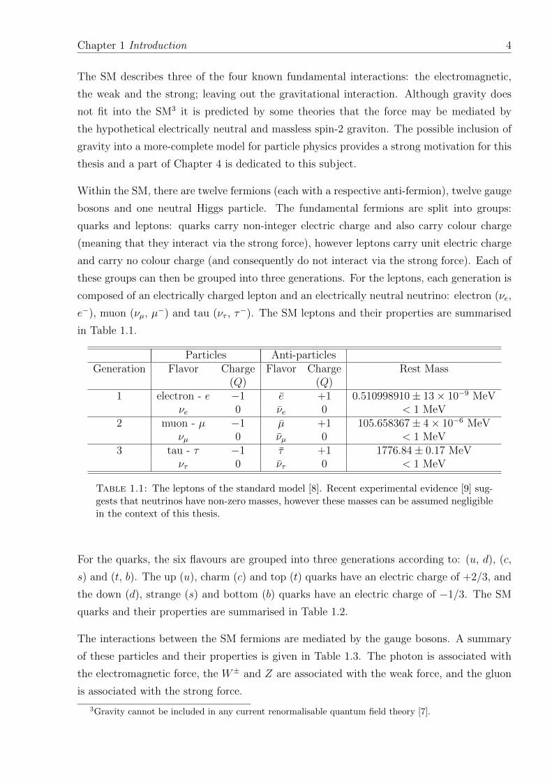
Within the SM, there are twelve fermions (each with a respective anti-fermion), twelve gauge
bosons and one neutral Higgs particle. The fundamental fermions are split into groups:
quarks and leptons: quarks carry non-integer electric charge and also carry colour charge
(meaning that they interact via the strong force), however leptons carry unit electric charge
and carry no colour charge (and consequently do not interact via the strong force). Each of
these groups can then be grouped into three generations. For the leptons, each generation is
composed of an electrically charged lepton and an electrically neutral neutrino: electron (νe,
e−), muon (νµ, µ−) and tau (ντ , τ−). The SM leptons and their properties are summarised
in Table 1.1.
Particles Anti-particlesGeneration Flavor Charge Flavor Charge Rest Mass
(Q) (Q)1 electron - e −1 e +1 0.510998910± 13× 10−9 MeV
νe 0 νe 0 < 1 MeV2 muon - µ −1 µ +1 105.658367± 4× 10⁻⁶ MeV
νµ 0 νµ 0 < 1 MeV3 tau - τ −1 τ +1 1776.84± 0.17 MeV
ντ 0 ντ 0 < 1 MeV
Table 1.1: The leptons of the standard model [8]. Recent experimental evidence [9] sug-gests that neutrinos have non-zero masses, however these masses can be assumed negligiblein the context of this thesis.
For the quarks, the six flavours are grouped into three generations according to: (u, d), (c,
s) and (t, b). The up (u), charm (c) and top (t) quarks have an electric charge of +2/3, and
the down (d), strange (s) and bottom (b) quarks have an electric charge of −1/3. The SM
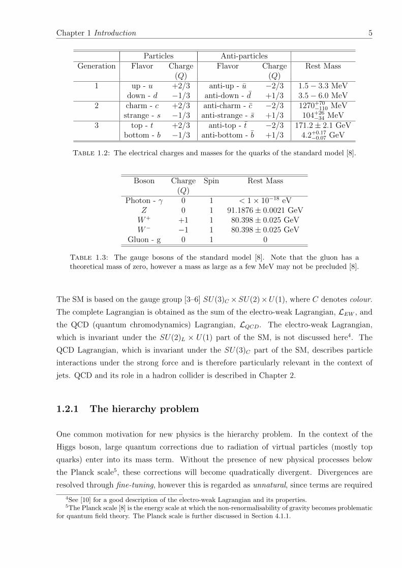
quarks and their properties are summarised in Table 1.2.
The interactions between the SM fermions are mediated by the gauge bosons. A summary
of these particles and their properties is given in Table 1.3. The photon is associated with
the electromagnetic force, the W± and Z are associated with the weak force, and the gluon
is associated with the strong force.
3Gravity cannot be included in any current renormalisable quantum field theory [7].
Chapter 1 Introduction 5
Particles Anti-particlesGeneration Flavor Charge Flavor Charge Rest Mass
(Q) (Q)1 up - u +2/3 anti-up - u −2/3 1.5− 3.3 MeV
down - d −1/3 anti-down - d +1/3 3.5− 6.0 MeV2 charm - c +2/3 anti-charm - c −2/3 1270+70
−110 MeVstrange - s −1/3 anti-strange - s +1/3 104+26
−34 MeV3 top - t +2/3 anti-top - t −2/3 171.2± 2.1 GeV
bottom - b −1/3 anti-bottom - b +1/3 4.2+0.17−0.07 GeV
Table 1.2: The electrical charges and masses for the quarks of the standard model [8].
Boson Charge Spin Rest Mass(Q)
Photon - γ 0 1 < 1× 10⁻¹⁸ eVZ 0 1 91.1876± 0.0021 GeVW+ +1 1 80.398± 0.025 GeVW− −1 1 80.398± 0.025 GeV
Gluon - g 0 1 0
Table 1.3: The gauge bosons of the standard model [8]. Note that the gluon has atheoretical mass of zero, however a mass as large as a few MeV may not be precluded [8].
The SM is based on the gauge group [3–6] SU(3)C ×SU(2)×U(1), where C denotes colour.
The complete Lagrangian is obtained as the sum of the electro-weak Lagrangian, LEW , and
the QCD (quantum chromodynamics) Lagrangian, LQCD. The electro-weak Lagrangian,
which is invariant under the SU(2)L × U(1) part of the SM, is not discussed here4. The
QCD Lagrangian, which is invariant under the SU(3)C part of the SM, describes particle
interactions under the strong force and is therefore particularly relevant in the context of
jets. QCD and its role in a hadron collider is described in Chapter 2.
1.2.1 The hierarchy problem
One common motivation for new physics is the hierarchy problem. In the context of the
Higgs boson, large quantum corrections due to radiation of virtual particles (mostly top
quarks) enter into its mass term. Without the presence of new physical processes below
the Planck scale5, these corrections will become quadratically divergent. Divergences are
resolved through fine-tuning, however this is regarded as unnatural, since terms are required
4See [10] for a good description of the electro-weak Lagrangian and its properties.5The Planck scale [8] is the energy scale at which the non-renormalisability of gravity becomes problematic
for quantum field theory. The Planck scale is further discussed in Section 4.1.1.
Chapter 1 Introduction 6
to cancel with a precision of ∼ O(M2D/M
2EW ) ∼ 10−32, where MEW is the Electro-weak
scale6. Alternatively, the need for fine-tuning can be avoided if new physics is in the order of
the Higgs scale. Contenders for such a theory include Supersymmetry [11], technicolor [12]
and extra dimensions (see Section 4.1), however the scope for some of these theories has
been limited by the recent observation of a new particle consistent with the SM Higgs
Boson [13, 14].
1.2.2 Current status: on the existence of the Higgs boson
On the 4th of July 2012, both the ATLAS and CMS experiments at CERN announced that
they had observed a new particle, consistent with a SM Higgs boson [13, 14].
The ATLAS result [13], based on 4.8 fb−1 of 7 TeV data and 5.8 fb−1 of 8 TeV data, observed
a neutral boson with measured mass 126 ± 0.4(stat) ± 0.4(sys) GeV with a significance of
5.9 standard deviations7.
The CMS result [14], based on 5.1 fb−1 of 7 TeV data and 5.3 fb−1 of 8 TeV data, observed
a neutral boson with measured mass 125.3± 0.4(stat)± 0.5(sys) GeV with a significance of
5.0 standard deviations.
Further work is currently in progress, which will aim to measure Higgs boson production in
all of its possible decay channels, and also to understand its properties.
1.3 Searches for New Physics using Dijet Angular Dis-
tributions in proton-proton collisions at√s = 7 TeV
collected with the ATLAS Detector
In this thesis, I will describe the most recent experimental results from searches for new
physical processes in the never-before explored territory of hadron collisions with a centre of
mass energy of 7 TeV. This thesis will concentrate on the analysis of collisions that result
in the production of two high energy jets. The production of particle jets is a dominant
process at the LHC and will thus provide the signal or define the measurement environment
6The Electro-weak scale is the typical energy associated with electro-weak interactions. A commonly
quoted value for the electro-weak scale is the vacuum expectation value of the Higgs field v = (GF√s)−1/2
=246 GeV [8].
7A significance of 5.9 standard deviations corresponds to a background fluctuation probability of 1.7 ×10⁻⁹.
Chapter 1 Introduction 7
for many analyses. A search for new physics signals within dijets is therefore also well-suited
for searches employing early LHC data.
As by far the most dominant process for producing such final states, the motivation, evidence
and simulation of Quantum Chromodynamics (QCD) will be introduced in Chapter 2.
As the experimental apparatus of this thesis, the LHC and, in particular, the ATLAS detector
are introduced in Chapter 3. The detector design and layout is discussed, however the
description is mostly limited to those components that contribute to the reconstruction of
jets.
In Chapter 4, the possibility of physics Beyond the Standard Model (BSM) will be ex-
plored. Three models are chosen that are predicted to have significant deviations from the
standard model dijet behaviour. These models, which are fundamentally different in their
phenomenology, are used as benchmark scenarios: allowing comparison between similar anal-
yses at other experiments. In the event of finding good agreement between data and the
SM, simulation of these BSM models allow one to constrain the possible values of certain
model parameters. This, in turn, guides theorists to explore the most likely models, given
our experimental observations.
Two models for quark sub-structure are described: these have been traditionally used as
benchmark models, such that exclusion limits from various collider experiments can be easily
compared. In addition, models including the extra spacial dimensions, aiming to explain
gravity’s relation to the SM, are discussed. As a relatively unexplored model, with a large
rate of decay to dijets, Quantum Black Holes are described in Section 4.2.
The methodology and performance of jet reconstruction in ATLAS is discussed in Chapter 5.
The journey from voltage measurements in the ATLAS calorimetry system to a full-calibrated
jet object, which is compared to a detailed Monte Carlo situation, is described.
Chapter 6 will then describe the phenomenology of the dominant signature of QCD: two-
jet final states, or more commonly, dijets. By combining angular, momentum and energy
information of the jets, an analysis objective is to explore as much of the dijet kinematic
phase space as possible. Variables are defined which enable one to explore this phase space,
with the aim testing agreement between data and simulation in the tails of the kinematic
reach, whilst reducing exposure to systematic uncertainties. Techniques detailed in this
section include a new method, developed with Dr. Frederik Ruehr (University of Arizona),
for probing mass-dependent changes in the angular behaviour of the dijet system. This
method, which is sensitive to both resonant new physics and threshold effects that operate
Chapter 1 Introduction 8
above a given energy scale, was first used in [15] and is the main analysis method for this
thesis.
In Chapter 7, the analysis procedure is described in detail. The selection of an unbiased
sample of dijet events from LHC collisions is described. Systematic uncertainties arising
from theoretical simulation of background process and experimental effects are considered
in full and their effects on the physics analysis are quantified. Environmental effects such as
detector malfunction and the high rate of proton-proton collisions are also discussed. Finally,
control distributions are produced in order to validate the simulated background processes.
Chapter 8, will discuss statistical interpretation of results from the analysis of 4.8 fb−1 of
proton-proton collisions at√s = 7 TeV. Emphasis is placed on a new and novel technique,
known as Fχ(mjj), which is sensitive to both a resonant excess of central dijet events, and
the slow onset of angular behaviour producing an excess of dijet events. In the event of good
agreement between data and the SM Monte Carlo prediction, limits are placed on selected
model parameters. The process for this limit setting is described in detail.
Chapter 9 will summarise and draw conclusions based on the previous chapters. Implica-
tions of results are discussed in both the immediate context of the LHC, and further: to
implications for physics, in general. Future work and areas for potential improvements in
the analysis are also discussed.
Finally, Chapter 10 outlines work performed as part of the ATLAS Tag Coordination group.
This work is independent of the physics analysis described in this thesis, and summarises
contributions made to the area of data management and coordination: foremost the devel-
opment of the RunBrowser interface for accessing ATLAS data based on the selection of
various LHC and detector conditions.
1.4 Author’s contribution
The work described in this thesis includes a combination of contributions from multiple
members of the ATLAS Collaboration. Most of the analysis, results and conclusions have
been performed by the Exotics Dijet Analysis team, of which I am a member, with the
support of the ATLAS Jet Performance Group. Throughout this thesis I endeavour to
reference particular individual contributions from my colleagues.
In this section I will attempt to outline, in chronological order, my contributions to the work
contained in this thesis, and related publications.
Chapter 1 Introduction 9
Although not the topic as this thesis, during the 2009 summer preceding the official beginning
of my DPhil, I worked on an ATLAS internal note [16] investigating the use of the charge
asymmetry in W+jets production as a new probe of parton distribution functions in different
kinematic regions at the LHC. This method is now being further developed for use within
ATLAS.
Each new member of the ATLAS collaboration must carry out ‘service work’ in order to
become a qualified author. I began this work at the beginning of my first year: working with
Dr. Elizabeth Gallas and the ATLAS Tag Coordination Group. The details of this work are
outlined in Chapter 10. This work involved developing a new web-interface - allowing ATLAS
users to locate portions of data which satisfy a variety of selection criteria. A portion of the
results from this work were presented in a poster session at the Computing in High Energy
Physics (CHEP) conference in Taipei, Taiwan in October 2010 [17–19]. The proceedings of
this contribution were published in [20].
Towards the end of my first year, I began to look at the first data coming from the LHC at√s = 7 TeV. In particular, I concentrated on trying to understand the rate and physics of
events that were being diverted into a separate ‘debug stream’ independent from the main
‘physics stream’ which contains events primarily designated for analysis. As the first person
to analyse this debug stream data, I was able to identify a bias for high-pT , high multiplicity
events to cause time-outs in the High-Level-Trigger (HLT) system. After further investiga-
tion, along with my supervisor Dr. Cigdem Issever, it was decided that these events should be
included in all physics analyses. This work contributed to many jet-based measurements re-
sulting in a number of publications for the International Conference in High-Energy Physics
(ICHEP)[21–24] and also the first ATLAS publications at√s = 7 TeV [25–27]. This in-
vestigation also led to an improvement in the on-line muon trigger algorithms [28], which
in-turn eliminated the bias for jet events to enter the debug stream.
At the beginning of my second year, I relocated to CERN for a long-term attachment. I
joined the Exotics dijet team, responsible for searching for evidence of new physics resulting
in two-jet final states. The search strategy for this team can be divided into two categories:
resonance searches and analysis of dijet angular distributions. I decided to concentrate on the
latter: since this method lends itself to searches for threshold effects such as extra-dimensions
and strong gravity described in Chapter 4.
I became a key analyst for analysis of the full 2010 data-set of 36.4 pb−1 resulting in a
publication at the beginning of 2011 [15]. Working with Dr. Frederik Ruehr (University of
Arizona) and Dr. Nele Boelaert (Neils Bohr Institute, Copenhagen), I was made responsible
for limits based on distributions with fine binning in angular distributions, and coarse binning
Chapter 1 Introduction 10
in mass. This publication also resulted in first limits on the Quantum Black Hole models [29]
described in Section 4.2 of this thesis. This paper was published in the New Journal of
Physics [15] and was subsequently selected by the journal editors for inclusion in the exclusive
‘Highlights of 2011’ 8 collection [30].
In 2011, I enjoyed further responsibility within the research group. Working again with
Dr. Frederik Ruehr (University of Arizona), I was responsible for limits based on a new
angular analysis strategy using the variable Fχ(mjj) (see Chapter 7). These results formed
a publication with 4.8 fb−1 of data, the analysis and results of which form the bulk of this
thesis. The results of this analysis were published in [31].
8Papers are chosen on the basis of referee endorsement, novelty, scientific impact and broadness of appeal.
Chapter 2
Collider physics and quantum
chromodynamics
Over the last century, much headway has been made in understanding the behaviour of
particles that interact through nature’s dominant force - the strong force. Beginning with
the first attempts to explain the observed spectra of hadrons (baryons and mesons) by G.
Zweig and M. Gell-Mann, the idea of the quark as a fundamental constituent of the hadrons,
was born. The postulation of only 3 flavours of quark: up, down and strange, was sufficient
to explain some of the observed phenomena - and even led to the prediction of the later
observed Ω−. We now know that there are six flavours of quark, with the discovery of the
charm, bottom and top - where the top quark was discovered as recently as 2005. The main
interest at the LHC lies in the interactions of the proton constituents: the quarks and gluons.
The theory concerning the interactions of these constituents is Quantum Chromodynamics
(QCD).
This chapter will introduce the motivation, theory and application of QCD - the theory
that describes the strong force. As the dominant orchestrator of the physical interactions
considered in this thesis, the evolution of the development of QCD and its experimental
confirmation over the years, will be briefly discussed. To start, the experimental motivations
for QCD will be discussed in Section 2.1, followed by an introduction to the theoretical
framework in Section 2.2. As a hadron-hadron collider at a new energy frontier, the LHC
presents a unique opportunity to test the accuracy of QCD in a never-before encountered
regime. The phenomenology of proton-proton collisions at the LHC will be introduced in
Section 2.3 and their simulation using Monte Carlo techniques is discussed in Section 2.4.
11
Chapter 2. Collider physics and quantum chromodynamics 12
2.1 Scattering experiments and the parton model
The idea that quarks carry a three-fold ‘colour’ charge was introduced in order to explain
the observation of particles such as the ∆++. This extra degree of freedom was required
in order to allow the ∆++ to have simultaneously the correct permutational symmetry and
satisfy Fermi-Dirac statistics.
Further progress was made through deep inelastic scattering experiments (discussed below),
where a high energy lepton is scattered from a hadron. A key factor to consider is the
wavelength, λ, of the probing particle, which is related to the transferred momentum Q2 by
λ ∼ 1√Q2. (2.1)
Therefore, a large momentum transfer is equivalent to a high resolution. J. D. Bjorken [32]
predicted that, in the limit of infinite Q2 (know as the deep inelastic limit), the hadronic
factor in the cross section would depend only only on the Lorentz-invariant ratio
x =Q2
2p · q (2.2)
where Q2 = −q2 = −(p − p′)2 is the difference between the initial (p) and final (p′) lepton
4-momentum. R. P. Feynman [33] interpreted this effect, known as ‘scaling’, as elastic
scatterings with constituents of the hadron that he called ‘partons’ : the parton model.
Bjorken’s x variable can be identified as the fraction of the longitudinal hadron momentum
carried by a given parton. This prediction was initially verified by a joint experiment of the
SLAC and MIT groups [34].
Subsequent data on deep inelastic scattering showed that the scattering cross-section also
varies with Q2 and that the carriers of electric charge within hadrons have spin 1/2 [35–38].
The experimental evidence suggests that the proton is made up from 3 valence quarks - two
up quarks and one down quark, along with a ‘sea’ of lower energy quark-anti-quark pairs
that continuously pair-produce and annihilate.
The contribution of each quark flavour is described by its momentum distribution function
q(x,Q2), where q(x,Q2)dx represents the probability of carrying a momentum fraction of the
parent hadron between x and x+dx, when the hadron is probed at scaleQ2. The combination
xfi(x,Q2) is known as the Parton Distribution Function (PDF) for the parton of flavour
i, where parton can refer to a quark, anti-quark or gluon. PDFs are further discussed in
Section 2.2.3.
Chapter 2. Collider physics and quantum chromodynamics 13
In terms of these momentum distributions functions, for the proton we have the following
sum rules: ∫ 1
0
uv(x,Q2) dx = 2,
∫ 1
0
dv(x,Q2) dx = 1, (2.3)
where uv and dv are the valence contributions to the patron momentum distribution func-
tions. It was also found that if one sums over the momenta of all quarks and anti-quarks in
the nucleon, expressed as Σ(x,Q2), then one observes that∫ 1
0
xΣ(x,Q2) dx ∼ 0.5. (2.4)
This, at first, unexpected result is now explained fully within the framework of QCD due to
the momentum carried by gluons: the gauge boson responsible for the strong force, which is
described by the theory of quantum chromodynamics.
2.2 Quantum chromodynamics
The strong force is described by Quantum Chromodynamics (QCD), which is a Quantum
Field Theory (QFT) based on the non-Abelian SU(3)C group, where C denotes the colour
charge, which is conserved under the strong force. The 8 generators of the SU(3)C group,
Aµa , a = 1, . . . , 8, result in the 8 types of gluon that are responsible for mediating the force.
The quantity gs is the QCD coupling constant.
The QCD Lagrangian density is given by
LQCD =∑f
ψif (iγµ(Dµ)ij −mfδij)ψ
jf −
1
4GaµνG
µνa , (2.5)
where ψf are the Dirac spinors of the different quark fields, which come in a colour triplet
representation with red (r), green (g) and blue (b), γµ are the Dirac spin matrices1, Dµ is
the covariant derivative (described below), and mf are the quark masses. The gluon field
strength tensor Gµνa is given by
Gµνa = ∂µAνa − ∂νAµa − igs[Aµa , Aνa] = ∂µAνa − ∂νAµa + gsf
bca A
µbA
νc , (2.6)
where Aa (a = 1, . . . , 8) are the eight gluon fields and fijk are the structure constants of the
SU(3)C group. The covariant derivative Dµ describes the interaction between the fields and
1For a good explanation of the Dirac spin matrices, and their role in the Dirac equation describing thebehaviour of particles with spin, see [2].
Chapter 2. Collider physics and quantum chromodynamics 14
is given by
Dµij = δij∂
µ + igs(ta)ijA
µa , (2.7)
where (ta)ij are the 3×3 hermitian matrices which, for the fundamental triplet representation
of SU(3), are (λa)ij/2, where λa are the Gell-Mann matrices2. The strength of the strong
interaction is determined by the coupling strength gs, which defines the strong coupling
constant αs = g2s/4π. The non-Abelian nature of the SU(3)C group leads to self-interaction
between the gluons - this can be seen in the Lagrangian as through the presence of the final
term in Equation 2.6.
2.2.1 Calculation of a cross-section from a Lagrangian
The Lagrangian in Equation 2.5, describing the theory of the strong force, is constructed such
that it is invariant under the symmetries of the SU(3) group. By respecting the symmetries
of the group, the theory is able to benefit from the mathematical representations of the
group, and their properties.
A prescription for calculating the rates for processes in any QFT was developed by Feynman.
Each term in the Lagrangian represents the interaction between various fields, and the
strength with which they interact. Feynman rules can be derived for each of the terms3.
Feynman diagrams are then used as a short hand to describe a calculation for one process
of a fixed order of perturbation theory. Perturbation theory is a method for calculating
the solution to an equation for which there is no analytical solution. Perturbation theory is
applicable if the problem at hand can be formulated by adding progressively “smaller” terms
to the mathematical description of the exactly solvable problem. This leads to an expression
for the desired solution in terms of a formal power series in some “small” parameter, α, that
quantifies the deviation from the exactly solvable problem. The precision of the perturbative
solution will then depend up on the number of terms that are included and the sizes of
additional terms. The highest power of α included in the expansion is know as the order 4
of the expansion. Figure 2.1 shows a few terms in the perturbative expansion of gluon
propagation (depicted by the curly lines) between two fermions (depicted by the straight
lines). Vertical displacement represents particle motion and time proceeds horizontally from
left to right. Each diagram carries a definite quantum mechanical amplitude for the process
that it represents. These amplitudes (commonly known as matrix elements) are constructed
2The Gell-Mann matrices are one representation of the SU(3) group. For further details, see [2].3These rules are derived using QFT. For a good introduction, see [39].4It is a common convention to refer to processes as ‘leading order’ (LO) or ‘next-to-leading order’ (NLO),
depending upon the order of α included in the perturbative expansion.
Chapter 2. Collider physics and quantum chromodynamics 15
from the Feynman rules, where each factor in the matrix element is formed from a term
associated with a feature of the diagram. Lines, of all sorts, represent the propagation
of particles, and vertices (points where two or more lines meet) represent the interaction
between particles. A full description of the Feynman rules associated with the SM is given
in [39].
Once a matrix element has been formed for a process, QFT provides a proscription for
arriving at a final cross-section: see [39] for a description of these calculations.
2.2.2 Singularities, renormalisation and asymptotic freedom
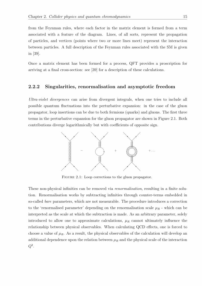
Ultra-violet divergences can arise from divergent integrals, when one tries to include all
possible quantum fluctuations into the perturbative expansion: in the case of the gluon
propagator, loop insertions can be due to both fermions (quarks) and gluons. The first three
terms in the perturbative expansion for the gluon propagator are shown in Figure 2.1. Both
contributions diverge logarithmically but with coefficients of opposite sign.
− + + . . .
Figure 2.1: Loop corrections to the gluon propagator.
These non-physical infinities can be removed via renormalisation, resulting in a finite solu-
tion. Renormalisation works by subtracting infinities through counter-terms embedded in
so-called bare parameters, which are not measurable. The procedure introduces a correction
to the ‘renormalised parameter’ depending on the renormalisation scale µR - which can be
interpreted as the scale at which the subtraction is made. As an arbitrary parameter, solely
introduced to allow one to approximate calculations, µR cannot ultimately influence the
relationship between physical observables. When calculating QCD effects, one is forced to
choose a value of µR. As a result, the physical observables of the calculation will develop an
additional dependence upon the relation between µR and the physical scale of the interaction
Q2.
Chapter 2. Collider physics and quantum chromodynamics 16
In the case of the QCD coupling constant, αs, the scale-dependence is described by the β
function:
Q∂αs∂Q≡ 2βQCD = − β0
2πα2s −
β1
4π2α3s −O(α4
s) (2.8)
where β0 = 11− 23nf and β1 = 51− 19
3nf and nf is the number of ‘active’ quark flavours at
the scale Q. Using Equation 2.8, one can calculate the value of αs at any scale Q, starting
from an experimental measurement of αs at a known scale µR, via
ln
(Q2
µ2R
)=
∫ αs(Q)
αs(µR)
dα
β(α). (2.9)
It is conventional to quote a value of the strong coupling constant at a mass of the Z-
boson, which is determined for a combination of various measurements. The current pre-
ferred value, based on next-to-next-to leading order perturbative calculations is given by
αs(MZ) = 0.1182 ± 0.0027 [40].
Calculating Equation 2.8 to LO in β(αs):
αs(Q2) =
α(µ2R)
1− α(µ2R)β0 ln(Q2/µ2
R), (2.10)
and making the substitution ln(Λ2QCD) = ln(µ2
R)− 1β0αs(µ2R)
gives
αs(Q2) =
1
β0 ln(Q2/Λ2QCD)
. (2.11)
From this expression, we can interpret ΛQCD as the scale at which αs becomes infinite. The
remarkable result that αs(Q2) → 0 as Q2 → ∞ is known as asymptotic freedom: when a
hadron is probed at low scales (corresponding to a low spatial resolution - see Equation 2.1)
we observe confined quarks, however for a high Q2 interaction (corresponding to a high
spatial resolution), such as deep inelastic scattering, we observe almost free quarks. The fact
that the strong force increases at larger length scales, results in the confinement of coloured
particles, i.e. it is not possible to produce a particle with colour charge in isolation and only
colour singlets composed of quarks and gluons can be observed. The increasing strength of
the strong force with distance, causes perturbative methods to break down as colour charges
move apart.
Chapter 2. Collider physics and quantum chromodynamics 17
2.2.3 Parton distribution functions
With an understanding of how QCD predicts the interactions between coloured partons, it
is possible to further-develop the parton model described in Section 2.1. In particular, one
can model the hadron as a dynamic object containing three valence quarks along a sea of
quarks and gluons which are continuously radiated and absorbed by each other. As described
above, through scattering experiments, it has been possible to measure the contribution of
each parton flavour to the parent hadron. By combining these experimental measurements
with theoretical tools provided by the QCD framework, we can deduce the phenomenology
of hadron interactions.
Within the proton, gluon emission gives a quark a large momentum kT with probability
proportional to αSdk2T/k
2T at large kT . In the collinear region (as kT → 0), this leads to
a non-physical divergence, since the perturbative QCD approximation is not valid in this
region. This divergence is removed by introducing a factorisation scale, µF : which can be
interpreted as an energy limit for describing the parton behaviour within the proton. In
a similar fashion to the renormalisation scale, the factorisation scale absorbs the collinear
divergences, resulting in a scale-dependent PDF.
Although perturbative QCD provides no absolute prediction for the PDF, it does dictate how
the PDF will evolve with Q2. This scale-evolution is described by the DGLAP5 equations,
which are coupled equations for the change of the quark, anti-quark and gluon densities
∂
∂ lnQ2
(qi(x,Q
2)
g(x,Q2)
)=αs(Q
2)
2π
∑j
∫ 1
x
dξ
ξ
(Pqiqj(
xξ, αs(Q
2)) Pqig(xξ, αs(Q
2))
Pgqj(xξ, αs(Q
2)) Pgg(xξ, αs(Q
2))
)(qj(ξ,Q
2)
g(ξ,Q2)
),
(2.12)
where the qi, qj are momentum distribution functions and are taken to include both quarks
and anti-quark distributions. The splitting function Pba(z,Q2) represents the probability
for parton a to radiate parton b, where b takes a fraction z of a’s momentum. In analogy
with the running coupling constant described in Section 2.2.2, the PDF must be measured
at some known scale µR before it can be evolved across the kinematic range. A combina-
tion of complementary measurements is employed from many scattering experiments6, has
allowed constraint of each of the individual parton PDFs over a range of values of x and
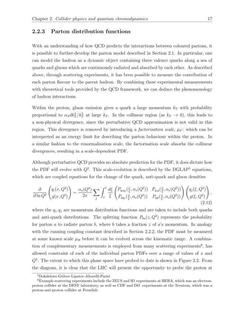
Q2. The extent to which this phase space have probed to date is shown in Figure 2.2. From
the diagram, it is clear that the LHC will present the opportunity to probe the proton at
5Dokshitzer-Gribov-Lipatov-Altarelli-Parisi6Example scattering experiments include the ZEUS and H1 experiments at HERA, which was an electron-
proton collider at the DESY laboratory, as well as CDF and DØ experiments at the Tevatron, which was aproton-anti-proton collider at Fermilab.
Chapter 2. Collider physics and quantum chromodynamics 18
previously un-explored regions of low-x and high-Q2. In addition, the overlap with previous
experiments allows the opportunity to test the validity of previous PDF fits that have been
derived from the collisions of different types of particle.
10-7
10-6
10-5
10-4
10-3
10-2
10-1
100
100
101
102
103
104
105
106
107
108
109
WJS2008
fixed
targetHERA
x1,2
= (M/1.96 TeV) exp(±y)
Q = M
Tevatron parton kinematics
M = 10 GeV
M = 100 GeV
M = 1 TeV
422 04y =
Q2 (
Ge
V2)
x
(a) Tevatron parton kinematics
10-7
10-6
10-5
10-4
10-3
10-2
10-1
100
100
101
102
103
104
105
106
107
108
109
fixed
targetHERA
x1,2
= (M/7 TeV) exp(±y)
Q = M
7 TeV LHC parton kinematics
M = 10 GeV
M = 100 GeV
M = 1 TeV
M = 7 TeV
66y = 40 224
Q2 (
Ge
V2)
x
WJS2010
(b) LHC parton kinematics at√s = 7 TeV
Figure 2.2: Parton kinematics in the x,Q2 plane for (a) Tevatron and (b) LHC collid-ers [41]. Kinematic ranges reached by the HERA collider and fixed target experiments areincluded for comparison. In the Figure, M indicates the mass of a given heavy particleproduced at rapidity y.
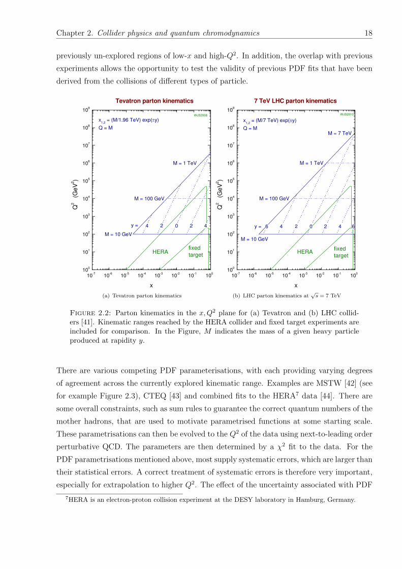
There are various competing PDF parameterisations, with each providing varying degrees
of agreement across the currently explored kinematic range. Examples are MSTW [42] (see
for example Figure 2.3), CTEQ [43] and combined fits to the HERA7 data [44]. There are
some overall constraints, such as sum rules to guarantee the correct quantum numbers of the
mother hadrons, that are used to motivate parametrised functions at some starting scale.
These parametrisations can then be evolved to the Q2 of the data using next-to-leading order
perturbative QCD. The parameters are then determined by a χ2 fit to the data. For the
PDF parametrisations mentioned above, most supply systematic errors, which are larger than
their statistical errors. A correct treatment of systematic errors is therefore very important,
especially for extrapolation to higher Q2. The effect of the uncertainty associated with PDF
7HERA is an electron-proton collision experiment at the DESY laboratory in Hamburg, Germany.
Chapter 2. Collider physics and quantum chromodynamics 19
parametrisations on the production of two-jet event considered in this analysis is discussed
in Section 7.4.
x-410 -310 -210 -110 1
)2xf
(x,Q
0
0.2
0.4
0.6
0.8
1
1.2
g/10
d
d
u
uss,cc,
2 = 10 GeV2Q
x-410 -310 -210 -110 1
)2xf
(x,Q
0
0.2
0.4
0.6
0.8
1
1.2
x-410 -310 -210 -110 1
)2xf
(x,Q
0
0.2
0.4
0.6
0.8
1
1.2
g/10
d
d
u
u
ss,
cc,
bb,
2 GeV4 = 102Q
x-410 -310 -210 -110 1
)2xf
(x,Q
0
0.2
0.4
0.6
0.8
1
1.2
MSTW 2008 NLO PDFs (68% C.L.)
Figure 2.3: Proton PDF distributions for√s = 7 TeV as a function of x according to
the MSTW collaboration [42] for up (u), down (d), charmed (c) and strange (s) quarksand their corresponding anti-quarks are shown. The left plot is for Q2 = 10 GeV2 and theright plot shows function for Q2 = 104 GeV2. Both plots also show distributions for g/10which is the gluon distribution scaled down by a factor of 10 in order to fit the same scaleas the other partons.
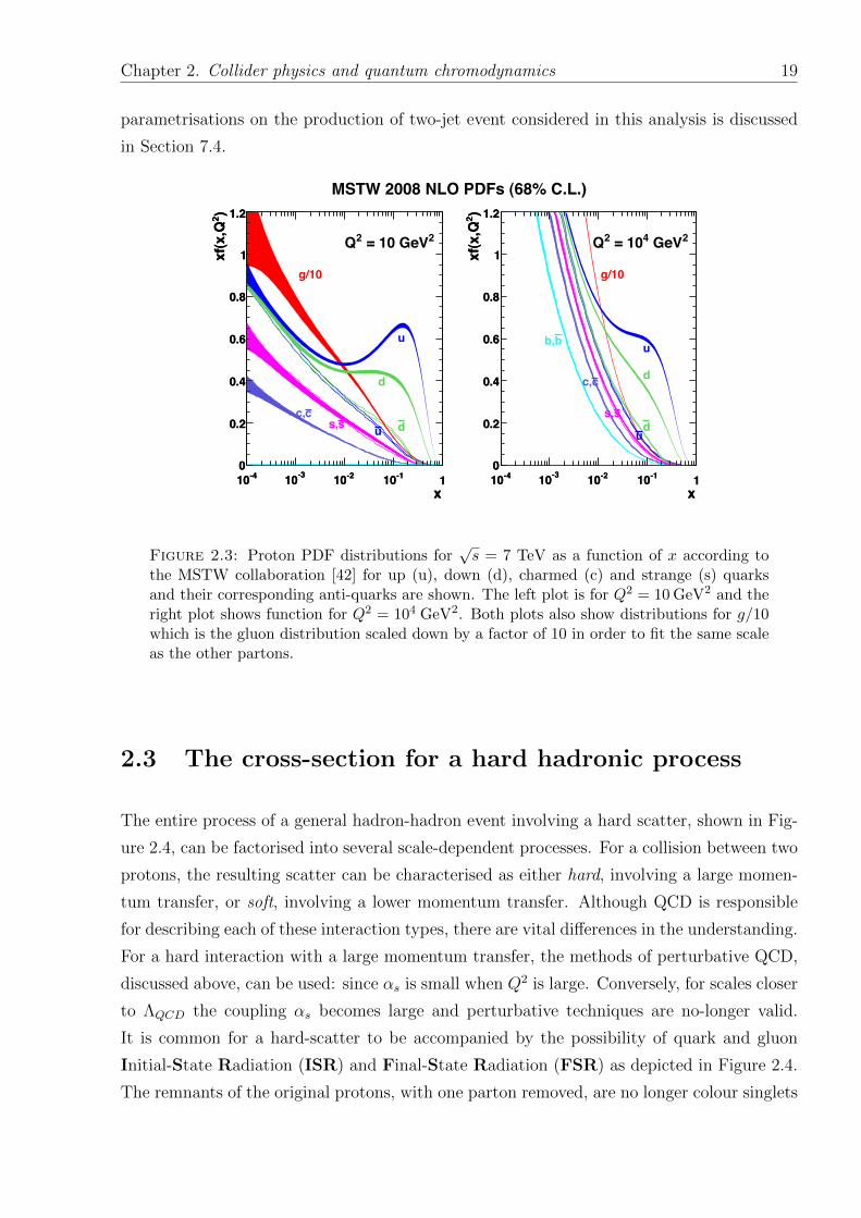
2.3 The cross-section for a hard hadronic process
The entire process of a general hadron-hadron event involving a hard scatter, shown in Fig-
ure 2.4, can be factorised into several scale-dependent processes. For a collision between two
protons, the resulting scatter can be characterised as either hard, involving a large momen-
tum transfer, or soft, involving a lower momentum transfer. Although QCD is responsible
for describing each of these interaction types, there are vital differences in the understanding.
For a hard interaction with a large momentum transfer, the methods of perturbative QCD,
discussed above, can be used: since αs is small when Q2 is large. Conversely, for scales closer
to ΛQCD the coupling αs becomes large and perturbative techniques are no-longer valid.
It is common for a hard-scatter to be accompanied by the possibility of quark and gluon
Initial-State Radiation (ISR) and Final-State Radiation (FSR) as depicted in Figure 2.4.
The remnants of the original protons, with one parton removed, are no longer colour singlets
Chapter 2. Collider physics and quantum chromodynamics 20
outgoing parton
outgoing parton
protonproton
underlying event
initial−state radiation
final−state radiation
underlying event
"Hard" scattering
Figure 2.4: Schematic for a proton-proton collision resulting in a hard-scatter betweentwo partons. Other possible interactions from initial and final state radiation and under-lying event are also included.
and will react to produce an underlying distribution of soft partons. This distribution is
known as the Underlying Event (UE).
The factorisation theorem [45] states that the hadron-hadron cross-section can be constructed
from a convolution of the calculable parton-level cross-section, with the parton momentum
distribution functions of the incident hadrons. This theorem is based on the differing time-
scale, energy-scale and distances involved in each of the terms. One may think of µF as
the scale that separates these two regimes and so separates what we refer to as the hard
interaction itself, and what could be referred to as the inner-workings of the proton, described
by the PDF. We therefore have a cross-section that is dependent upon two scales: the
renormalisation scale µR is associated with the limited precision of hard scatter calculations
in αs; and the factorisation scale µF is the scale associated with the partons within the
proton. We summarise this in the expression for the cross-section:
dσhard(pA, pB, Q2) =
∑ab
∫dxadxb fa/A(xa, µ
2F )fb/B(xb, µ
2F ) dσab→cd(αs(µ
2R), Q2/µ2
R) (2.13)
where dσab→cd is the parton-parton cross-section at a hard scale Q2 and fa/A is the parton
momentum density of a parton a in hadron A at a factorisation scale µF . The initial parton
momenta are given by pa = xapA and pb = xbpB.
Given that it is not possible to perform calculations to all orders, the final cross-section
will retain some dependence on the renormalisation scale (µR) and the factorisation scale
(µF ). The variation of these parameters will therefore present a systematic uncertainty on
Chapter 2. Collider physics and quantum chromodynamics 21
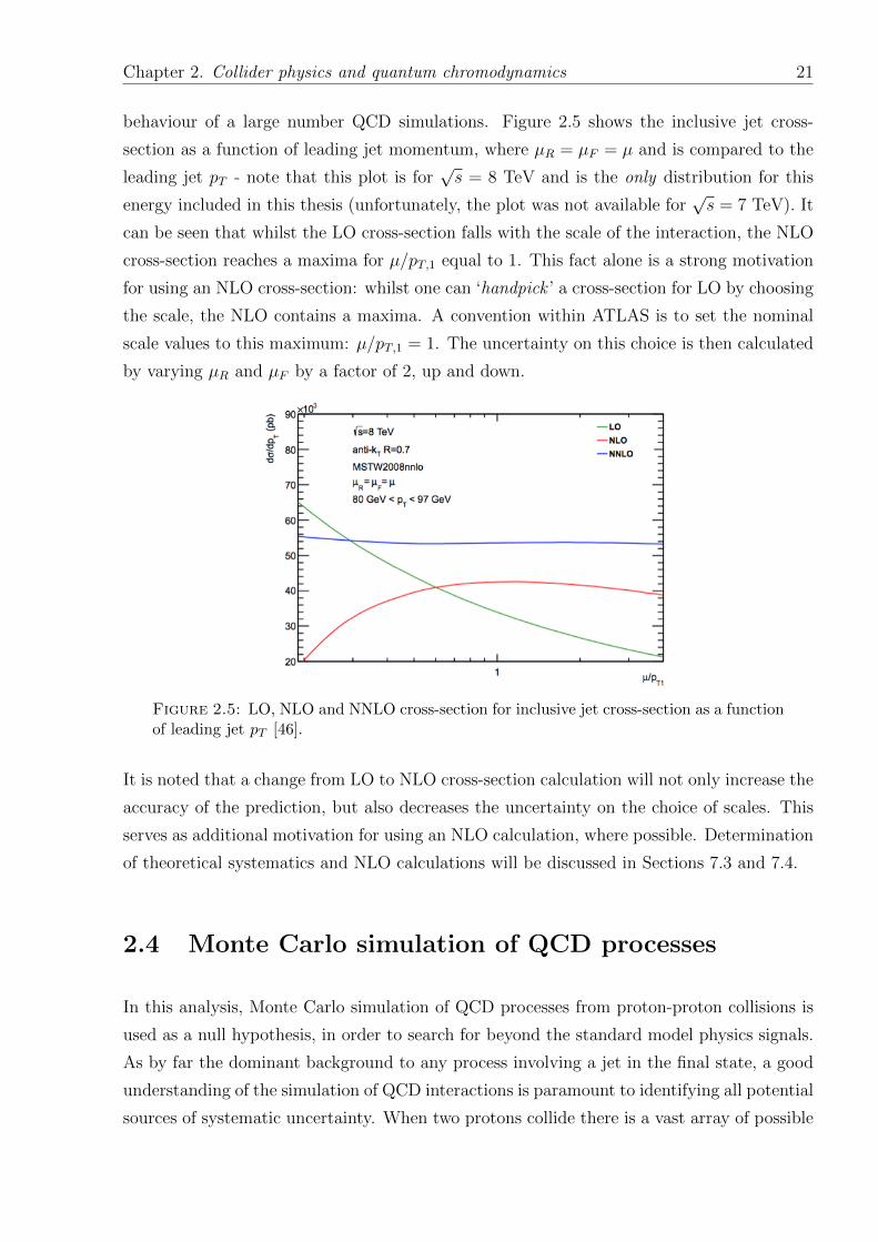
behaviour of a large number QCD simulations. Figure 2.5 shows the inclusive jet cross-
section as a function of leading jet momentum, where µR = µF = µ and is compared to the
leading jet pT - note that this plot is for√s = 8 TeV and is the only distribution for this
energy included in this thesis (unfortunately, the plot was not available for√s = 7 TeV). It
can be seen that whilst the LO cross-section falls with the scale of the interaction, the NLO
cross-section reaches a maxima for µ/pT,1 equal to 1. This fact alone is a strong motivation
for using an NLO cross-section: whilst one can ‘handpick ’ a cross-section for LO by choosing
the scale, the NLO contains a maxima. A convention within ATLAS is to set the nominal
scale values to this maximum: µ/pT,1 = 1. The uncertainty on this choice is then calculated
by varying µR and µF by a factor of 2, up and down.
Figure 2.5: LO, NLO and NNLO cross-section for inclusive jet cross-section as a functionof leading jet pT [46].
It is noted that a change from LO to NLO cross-section calculation will not only increase the
accuracy of the prediction, but also decreases the uncertainty on the choice of scales. This
serves as additional motivation for using an NLO calculation, where possible. Determination
of theoretical systematics and NLO calculations will be discussed in Sections 7.3 and 7.4.
2.4 Monte Carlo simulation of QCD processes
In this analysis, Monte Carlo simulation of QCD processes from proton-proton collisions is
used as a null hypothesis, in order to search for beyond the standard model physics signals.
As by far the dominant background to any process involving a jet in the final state, a good
understanding of the simulation of QCD interactions is paramount to identifying all potential
sources of systematic uncertainty. When two protons collide there is a vast array of possible
Chapter 2. Collider physics and quantum chromodynamics 22
outcomes, with the probability of each outcome described by Equation 2.13. Therefore, in
order to deduce any significant conclusions, a very large number of proton-proton collisions
needs to be considered. The LHC will provide billions of proton-proton collisions that will
be recorded for analysis. In order to quantify the agreement between the data and theory,
one must therefore simulate a large number of Monte Carlo processes for comparison. The
generation of these Monte Carlo events can be split into multiple steps outlined below.
The nature of the incoming partons taking part in the hard subprocess, i.e. their flavour and
momentum distributions (described in Section 2.2.3), determine the main characteristics of
the event. One parton from each beam particle initiates a shower of partons: the remainder
of which contribute to the beam remnants, or may take part in multiple parton interactions.
2.4.1 Simulation of the hard scattering process
The leading order cross-sections for a given physics process can be calculated using Equa-
tion 2.13. Calculations for NLO effects (and beyond) for the hard scattering are notoriously
difficult - and due to the large scale of the interaction, it is usually sufficient to restrict the
calculation to leading order. However, in some areas of phase-space, next-to-leading order
effects (and beyond) can be non-negligible Although some NLO MC event generators are
available for some subprocesses (e.g. Powheg-Box [47–49]), these have taken many years
to develop and are still not completely trusted.
2.4.2 Parton showering
When two coloured particles exist in either the initial or final state, there is a finite probability
of either of the particles radiating another parton. As seen in Section 2.2.2, this can lead to
either infra-red or collinear divergences. An alternative to summing higher order terms from
the DGLAP formalism is provided by some Monte Carlo generators. In the parton shower
approach, e.g. used by Pythia [50], the few partons produced in the hard interactions are
related to partons close to the QCD scale ΛQCD. At this scale a phenomenological model
can then be used to perform the hadronisation of final state partons. The evolution can
be expressed in Sudakov form factors, which give the probability that a parton evolves to a
higher scale than a given value8. For a further discussion of Sudakov form factors and their
behaviour at different scales, see [51]. Parton showers provide a very good description of
8In Pythia 6.4, which is used in this thesis, the relative transverse momentum of the two partons is usedas the scale of choice.
Chapter 2. Collider physics and quantum chromodynamics 23
collinear and infra-red emission, while the fixed order calculations can be used for the widely
separated partons. Care must be taken to avoid double-counting in kinematics regions where
both techniques overlap.
2.4.3 Hadronisation of coloured particles in the final state
Hadronisation is the process by which colour neutral hadrons are created from outgoing
quark and gluons from the final state. As coloured particles move apart, the strong interac-
tion between them increases. The potential between the two partons increases linearly with
their separation, until there is sufficient energy to produce a new parton pair. This new par-
ton pair is then able to neutralise the colour charge of each of the initial partons producing
a hadronic state. Within a collision experiment, all outgoing partons will therefore undergo
parton showering and transform into hadrons. These hadrons will in-turn form jets - sprays
of particles, which to a good approximation point in the direction of the original high energy
parton. This process is called hadronisation and results in the experimentally measurable
jets. As the hadronisation process evolves, the scale of the parton radiation will decrease
leading to a larger strong coupling - perturbative methods cannot therefore be used to de-
scribe the hadronisation process and phenomenological models must be relied upon instead.
Models describing hadronisation include the Lund string model [52] (used in e.g. Pythia)
and the cluster model [53] (used in e.g. Herwig [54]). In each of these models, colour singlet
structures are formed from colour connected partons and are decayed into hadrons, whilst
ensuring that energy and momentum are conserved.
2.5 QCD Monte Carlo simulation used in this thesis
The background process considered in this thesis will consist of events generated at leading-
order for the hard scattering process by the Pythia generator. Pythia [50] is a complete,
multi-purpose event generator with leading-order matrix elements. This program has be-
come the standard across multiple experiments due to its wide range of simulated processes
from both within and beyond the standard model. The QCD hard scattering interactions
are simulated using the Pythia 6.4 [50] event generator with the ATLAS AUET2B LO**
tune [55] which uses the MRSTMCal [56] modified leading-order (LO**) parton distribution
functions (PDF).
As shown Figures 7.12(c) and 7.12(d), the inclusive jet cross-section features a steep drop
with jet pT : the simulation of the QCD process is therefore split between certain regions
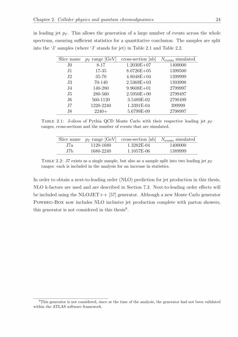
Chapter 2. Collider physics and quantum chromodynamics 24
in leading jet pT . This allows the generation of a large number of events across the whole
spectrum, ensuring sufficient statistics for a quantitative conclusion. The samples are split
into the ‘J’ samples (where ‘J’ stands for jet) in Table 2.1 and Table 2.2.
Slice name pT range [GeV] cross-section [nb] Nevents simulatedJ0 8-17 1.2030E+07 1400000J1 17-35 8.0726E+05 1399500J2 35-70 4.8048E+04 1399999J3 70-140 2.5369E+03 1393998J4 140-280 9.9608E+01 2799997J5 280-560 2.5950E+00 2799497J6 560-1120 3.5489E-02 2798499J7 1220-2240 1.3391E-04 399999J8 2240+ 5.6799E-09 2798997
Table 2.1: J-slices of Pythia QCD Monte Carlo with their respective leading jet pTranges, cross-sections and the number of events that are simulated.
Slice name pT range [GeV] cross-section [nb] Nevents simulatedJ7a 1120-1680 1.3282E-04 1400000J7b 1680-2240 1.1057E-06 1389999
Table 2.2: J7 exists as a single sample, but also as a sample split into two leading jet pTranges: each is included in the analysis for an increase in statistics.
In order to obtain a next-to-leading order (NLO) prediction for jet production in this thesis,
NLO k-factors are used and are described in Section 7.3. Next-to-leading order effects will
be included using the NLOJET++ [57] generator. Although a new Monte Carlo generator
Powheg-Box now includes NLO inclusive jet production complete with parton showers,
this generator is not considered in this thesis9.
9This generator is not considered, since at the time of the analysis, the generator had not been validatedwithin the ATLAS software framework.
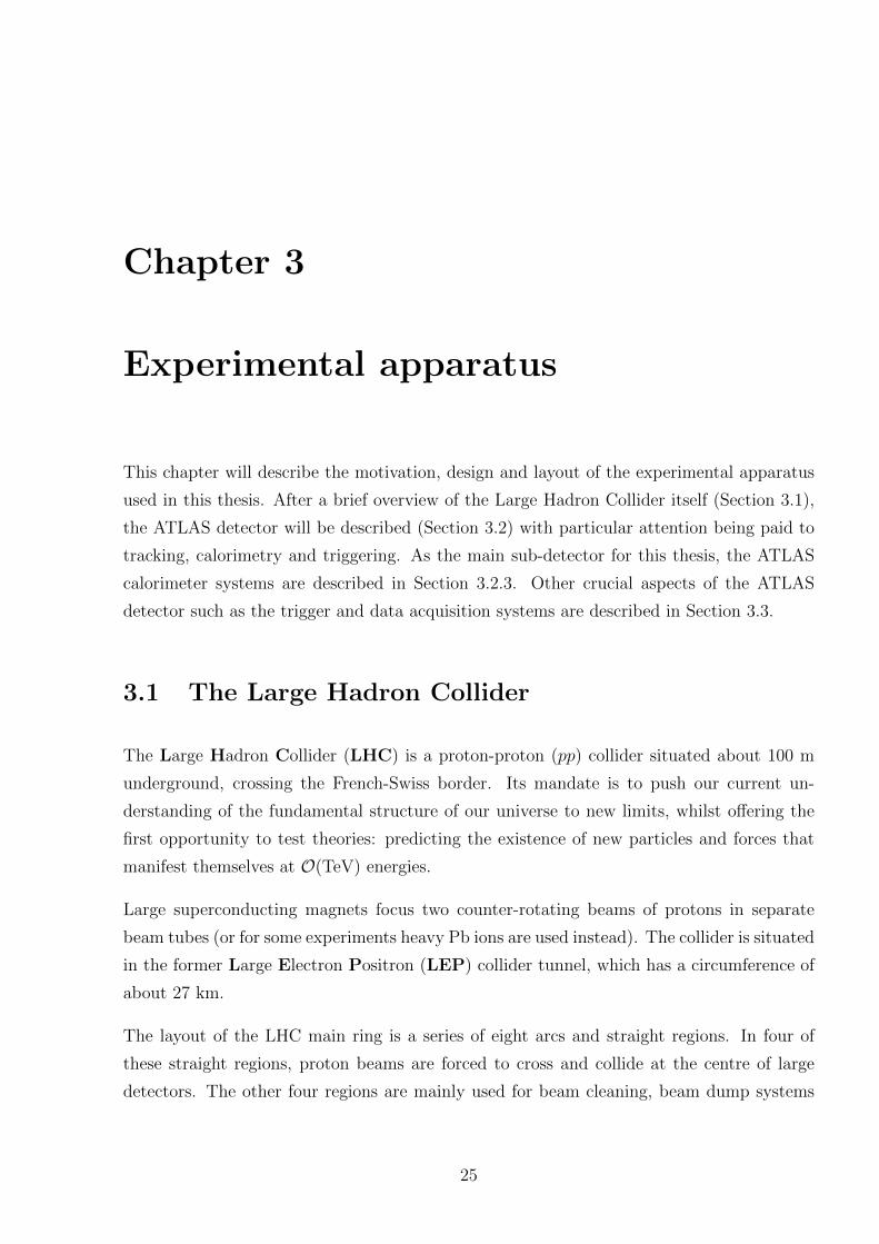
Chapter 3
Experimental apparatus
This chapter will describe the motivation, design and layout of the experimental apparatus
used in this thesis. After a brief overview of the Large Hadron Collider itself (Section 3.1),
the ATLAS detector will be described (Section 3.2) with particular attention being paid to
tracking, calorimetry and triggering. As the main sub-detector for this thesis, the ATLAS
calorimeter systems are described in Section 3.2.3. Other crucial aspects of the ATLAS
detector such as the trigger and data acquisition systems are described in Section 3.3.
3.1 The Large Hadron Collider
The Large Hadron Collider (LHC) is a proton-proton (pp) collider situated about 100 m
underground, crossing the French-Swiss border. Its mandate is to push our current un-
derstanding of the fundamental structure of our universe to new limits, whilst offering the
first opportunity to test theories: predicting the existence of new particles and forces that
manifest themselves at O(TeV) energies.
Large superconducting magnets focus two counter-rotating beams of protons in separate
beam tubes (or for some experiments heavy Pb ions are used instead). The collider is situated
in the former Large Electron Positron (LEP) collider tunnel, which has a circumference of
about 27 km.
The layout of the LHC main ring is a series of eight arcs and straight regions. In four of
these straight regions, proton beams are forced to cross and collide at the centre of large
detectors. The other four regions are mainly used for beam cleaning, beam dump systems
25
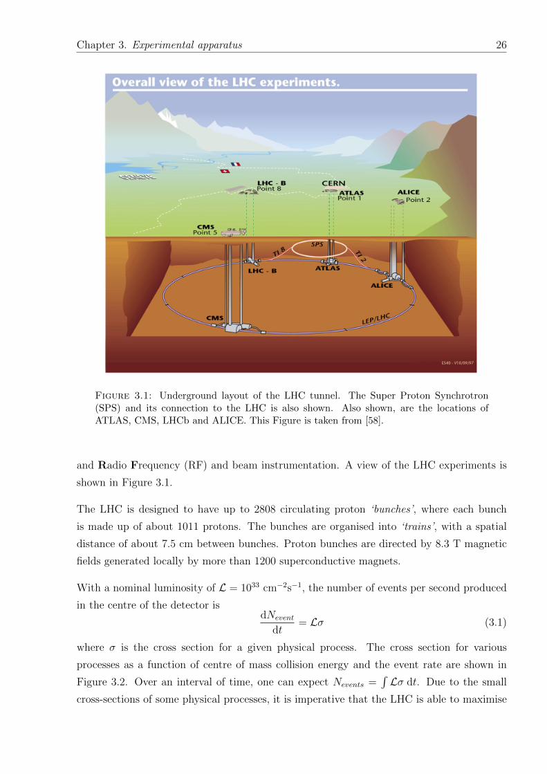
Chapter 3. Experimental apparatus 26
Figure 3.1: Underground layout of the LHC tunnel. The Super Proton Synchrotron(SPS) and its connection to the LHC is also shown. Also shown, are the locations ofATLAS, CMS, LHCb and ALICE. This Figure is taken from [58].
and Radio Frequency (RF) and beam instrumentation. A view of the LHC experiments is
shown in Figure 3.1.
The LHC is designed to have up to 2808 circulating proton ‘bunches’, where each bunch
is made up of about 1011 protons. The bunches are organised into ‘trains’, with a spatial
distance of about 7.5 cm between bunches. Proton bunches are directed by 8.3 T magnetic
fields generated locally by more than 1200 superconductive magnets.
With a nominal luminosity of L = 1033 cm−2s−1, the number of events per second produced
in the centre of the detector isdNevent
dt= Lσ (3.1)
where σ is the cross section for a given physical process. The cross section for various
processes as a function of centre of mass collision energy and the event rate are shown in
Figure 3.2. Over an interval of time, one can expect Nevents =∫Lσ dt. Due to the small
cross-sections of some physical processes, it is imperative that the LHC is able to maximise
Chapter 3. Experimental apparatus 27
0.1 1 1010
-7
10-6
10-5
10-4
10-3
10-2
10-1
100
101
102
103
104
105
106
107
108
109
10-7
10-6
10-5
10-4
10-3
10-2
10-1
100
101
102
103
104
105
106
107
108
109
!!!!ZZ
!!!!WW
!!!!WH
!!!!VBF
MH=125 GeV
WJS2012
!!!!jet
(ET
jet > 100 GeV)
!!!!jet
(ET
jet > """"s/20)
!!!!ggH
LHCTevatron
eve
nts
/ s
ec f
or L
= 1
03
3 c
m-2s
-1
!!!!b
!!!!tot
proton - (anti)proton cross sections
!!!!W
!!!!Z
!!!!t
!
!
!
!
(( ((nb
)) ))
""""s (TeV)
Figure 3.2: Cross section for various processes as a function of centre of mass collisionenergy and the event rate [41].
its delivered luminosity. The calculation of the instantaneous luminosity delivered by the
LHC is discussed in [59].
The detectors at the four separated interaction points are named ATLAS (A Toroidal LHC
ApparatuS), CMS (Compact Muon Solenoid), ALICE (A Large Ion Collider Experiment)
and LHCb (LHC beauty). ATLAS and CMS are general purpose detectors designed to
cover a multitude of physics: ranging from the confirmation of Standard Model physics to
the search for new particles and forces. ALICE is a heavy ion collision detector and LHCb
is specially designed for b-physics study1.
Two further experiments operating at the LHC are TOTEM (TOTal cross section, Elastic
scattering and diffraction dissociation Measurement at the LHC), designed for precise mea-
surement of the proton-proton interaction cross-section, and LHCf (LHC forward), de-
signed to study of neutral particles, produced from proton-proton collisions at very small
angles to the beam line.
1This involves studies of particles which contain b quarks which allow us to study the phenomenon ofCharge-Parity (CP) symmetry violation.
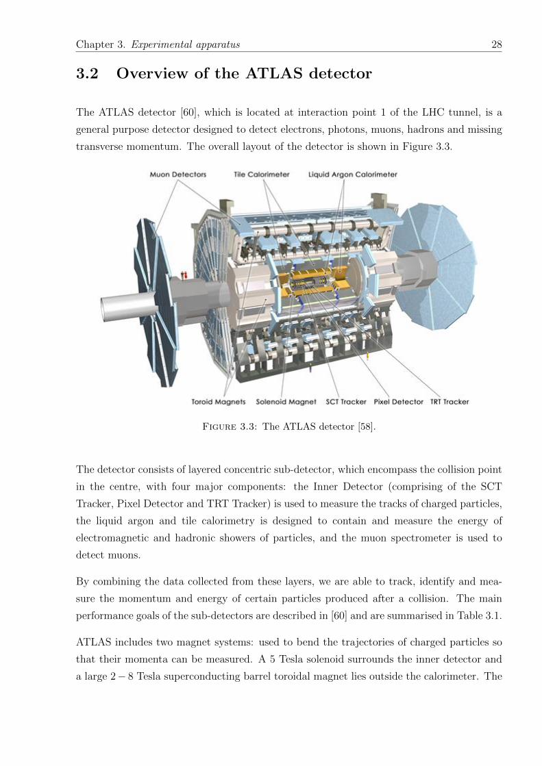
Chapter 3. Experimental apparatus 28
3.2 Overview of the ATLAS detector
The ATLAS detector [60], which is located at interaction point 1 of the LHC tunnel, is a
general purpose detector designed to detect electrons, photons, muons, hadrons and missing
transverse momentum. The overall layout of the detector is shown in Figure 3.3.
Figure 3.3: The ATLAS detector [58].
The detector consists of layered concentric sub-detector, which encompass the collision point
in the centre, with four major components: the Inner Detector (comprising of the SCT
Tracker, Pixel Detector and TRT Tracker) is used to measure the tracks of charged particles,
the liquid argon and tile calorimetry is designed to contain and measure the energy of
electromagnetic and hadronic showers of particles, and the muon spectrometer is used to
detect muons.
By combining the data collected from these layers, we are able to track, identify and mea-
sure the momentum and energy of certain particles produced after a collision. The main
performance goals of the sub-detectors are described in [60] and are summarised in Table 3.1.
ATLAS includes two magnet systems: used to bend the trajectories of charged particles so
that their momenta can be measured. A 5 Tesla solenoid surrounds the inner detector and
a large 2− 8 Tesla superconducting barrel toroidal magnet lies outside the calorimeter. The
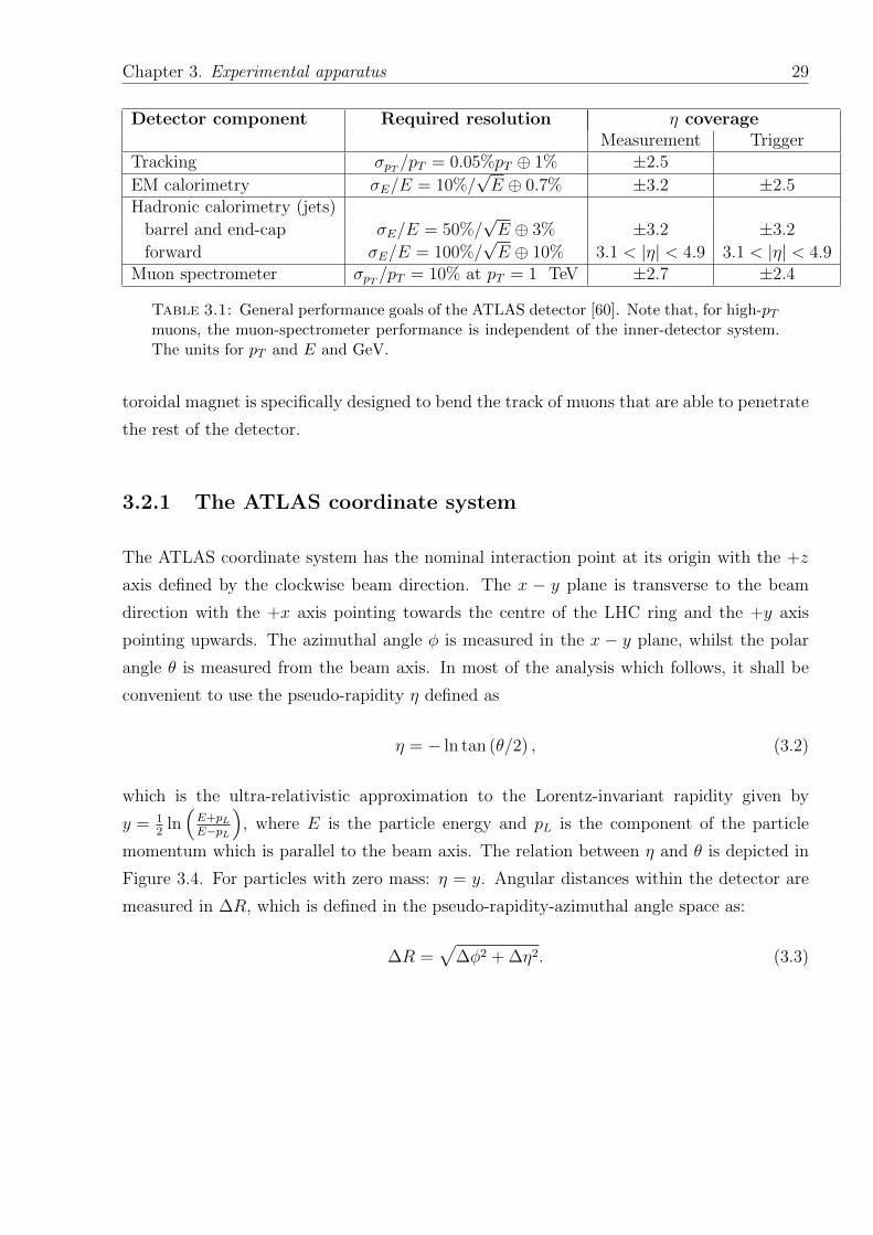
Chapter 3. Experimental apparatus 29
Detector component Required resolution η coverageMeasurement Trigger
Tracking σpT /pT = 0.05%pT ⊕ 1% ±2.5
EM calorimetry σE/E = 10%/√E ⊕ 0.7% ±3.2 ±2.5
Hadronic calorimetry (jets)
barrel and end-cap σE/E = 50%/√E ⊕ 3% ±3.2 ±3.2
forward σE/E = 100%/√E ⊕ 10% 3.1 < |η| < 4.9 3.1 < |η| < 4.9
Muon spectrometer σpT /pT = 10% at pT = 1 TeV ±2.7 ±2.4
Table 3.1: General performance goals of the ATLAS detector [60]. Note that, for high-pTmuons, the muon-spectrometer performance is independent of the inner-detector system.The units for pT and E and GeV.
toroidal magnet is specifically designed to bend the track of muons that are able to penetrate
the rest of the detector.
3.2.1 The ATLAS coordinate system
The ATLAS coordinate system has the nominal interaction point at its origin with the +z
axis defined by the clockwise beam direction. The x − y plane is transverse to the beam
direction with the +x axis pointing towards the centre of the LHC ring and the +y axis
pointing upwards. The azimuthal angle φ is measured in the x − y plane, whilst the polar
angle θ is measured from the beam axis. In most of the analysis which follows, it shall be
convenient to use the pseudo-rapidity η defined as
η = − ln tan (θ/2) , (3.2)
which is the ultra-relativistic approximation to the Lorentz-invariant rapidity given by
y = 12
ln(E+pLE−pL
), where E is the particle energy and pL is the component of the particle
momentum which is parallel to the beam axis. The relation between η and θ is depicted in
Figure 3.4. For particles with zero mass: η = y. Angular distances within the detector are
measured in ∆R, which is defined in the pseudo-rapidity-azimuthal angle space as:
∆R =√
∆φ2 + ∆η2. (3.3)
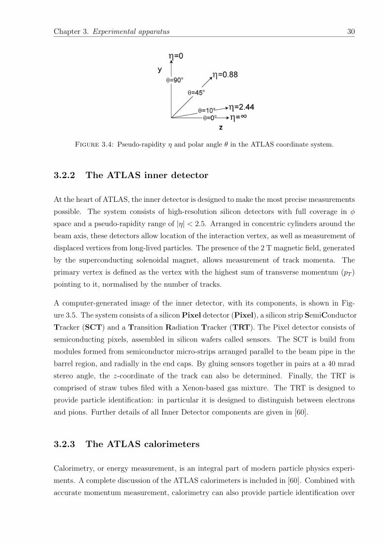
Chapter 3. Experimental apparatus 30
Figure 3.4: Pseudo-rapidity η and polar angle θ in the ATLAS coordinate system.
3.2.2 The ATLAS inner detector
At the heart of ATLAS, the inner detector is designed to make the most precise measurements
possible. The system consists of high-resolution silicon detectors with full coverage in φ
space and a pseudo-rapidity range of |η| < 2.5. Arranged in concentric cylinders around the
beam axis, these detectors allow location of the interaction vertex, as well as measurement of
displaced vertices from long-lived particles. The presence of the 2 T magnetic field, generated
by the superconducting solenoidal magnet, allows measurement of track momenta. The
primary vertex is defined as the vertex with the highest sum of transverse momentum (pT )
pointing to it, normalised by the number of tracks.
A computer-generated image of the inner detector, with its components, is shown in Fig-
ure 3.5. The system consists of a silicon Pixel detector (Pixel), a silicon strip SemiConductor
Tracker (SCT) and a Transition Radiation Tracker (TRT). The Pixel detector consists of
semiconducting pixels, assembled in silicon wafers called sensors. The SCT is build from
modules formed from semiconductor micro-strips arranged parallel to the beam pipe in the
barrel region, and radially in the end caps. By gluing sensors together in pairs at a 40 mrad
stereo angle, the z-coordinate of the track can also be determined. Finally, the TRT is
comprised of straw tubes filed with a Xenon-based gas mixture. The TRT is designed to
provide particle identification: in particular it is designed to distinguish between electrons
and pions. Further details of all Inner Detector components are given in [60].
3.2.3 The ATLAS calorimeters
Calorimetry, or energy measurement, is an integral part of modern particle physics experi-
ments. A complete discussion of the ATLAS calorimeters is included in [60]. Combined with
accurate momentum measurement, calorimetry can also provide particle identification over
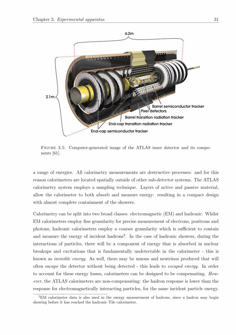
Chapter 3. Experimental apparatus 31
Figure 3.5: Computer-generated image of the ATLAS inner detector and its compo-nents [61].
a range of energies. All calorimetry measurements are destructive processes: and for this
reason calorimeters are located spatially outside of other sub-detector systems. The ATLAS
calorimetry system employs a sampling technique. Layers of active and passive material,
allow the calorimeter to both absorb and measure energy: resulting in a compact design
with almost complete containment of the showers.
Calorimetry can be split into two broad classes: electromagnetic (EM) and hadronic. Whilst
EM calorimeters employ fine granularity for precise measurement of electrons, positrons and
photons, hadronic calorimeters employ a coarser granularity which is sufficient to contain
and measure the energy of incident hadrons2. In the case of hadronic showers, during the
interactions of particles, there will be a component of energy that is absorbed in nuclear
breakups and excitations that is fundamentally undetectable in the calorimeter - this is
known as invisible energy. As well, there may be muons and neutrinos produced that will
often escape the detector without being detected - this leads to escaped energy. In order
to account for these energy losses, calorimeters can be designed to be compensating. How-
ever, the ATLAS calorimeters are non-compensating: the hadron response is lower than the
response for electromagnetically interacting particles, for the same incident particle energy.
2EM calorimeter data is also used in the energy measurement of hadrons, since a hadron may beginshowing before it has reached the hadronic Tile calorimeter.
Chapter 3. Experimental apparatus 32
The correct energy scale for hadronic interactions is restored ‘offline’ - at the data analysis
level. The techniques employed to calculate this Jet Energy Scale, (JES) are discussed in
Section 5.4.
Figure 3.6: Layout of the ATLAS calorimetry system [58].
The ATLAS calorimetry is comprised of six subsystems divided into barrel, extended bar-
rel and end-cap regions (See Figure 3.6). The barrel region consists of a Liquid Argon
(LAr) electromagnetic calorimeter and presampler, and a scintillating plastic TILE hadronic
calorimeter (TILE). The end-cap calorimeters are all based on LAr sampling technology: an
electromagnetic presampler and ElectroMagnatic End-Cap (EMEC), the Hadronic End-
Cap (HEC) and the Forward CALorimeter (FCAL). An extended barrel region of hadronic
calorimeter surrounds the end cap calorimeters, as seen in Figure 3.6.
The calorimeters are designed to provide a good containment of electromagnetic and hadronic
showers: otherwise a shower may punch-through into the muon system. The calorimeter
depth is tailored to limit this punch-through. The total thickness of the EM calorimeter is
≈ 22 radiation lengths (X0) in the barrel and ≈ 24 X0 in the end caps: where 9.7 interaction
lengths (λ) of active calorimeter material in the barrel (and 11 λ in the end-cap) is adequate
to provide good resolution for high-energy jets - see Table 3.1.
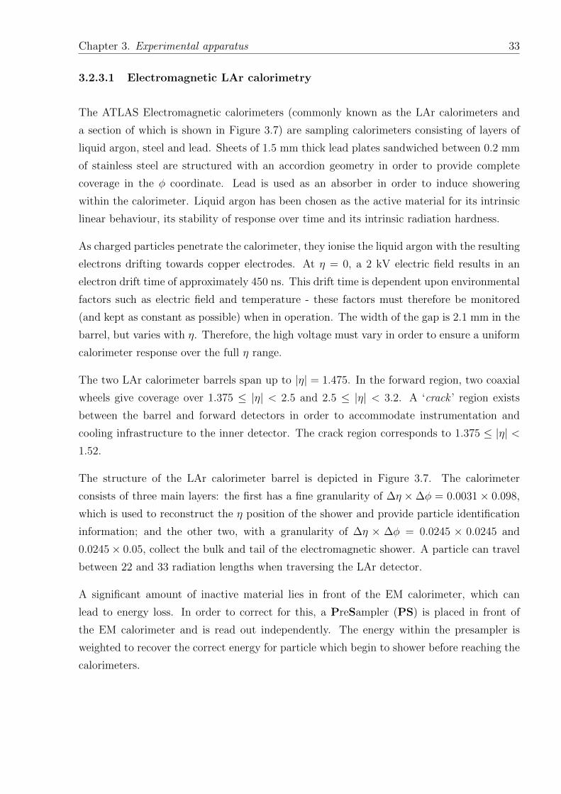
Chapter 3. Experimental apparatus 33
3.2.3.1 Electromagnetic LAr calorimetry
The ATLAS Electromagnetic calorimeters (commonly known as the LAr calorimeters and
a section of which is shown in Figure 3.7) are sampling calorimeters consisting of layers of
liquid argon, steel and lead. Sheets of 1.5 mm thick lead plates sandwiched between 0.2 mm
of stainless steel are structured with an accordion geometry in order to provide complete
coverage in the φ coordinate. Lead is used as an absorber in order to induce showering
within the calorimeter. Liquid argon has been chosen as the active material for its intrinsic
linear behaviour, its stability of response over time and its intrinsic radiation hardness.
As charged particles penetrate the calorimeter, they ionise the liquid argon with the resulting
electrons drifting towards copper electrodes. At η = 0, a 2 kV electric field results in an
electron drift time of approximately 450 ns. This drift time is dependent upon environmental
factors such as electric field and temperature - these factors must therefore be monitored
(and kept as constant as possible) when in operation. The width of the gap is 2.1 mm in the
barrel, but varies with η. Therefore, the high voltage must vary in order to ensure a uniform
calorimeter response over the full η range.
The two LAr calorimeter barrels span up to |η| = 1.475. In the forward region, two coaxial
wheels give coverage over 1.375 ≤ |η| < 2.5 and 2.5 ≤ |η| < 3.2. A ‘crack ’ region exists
between the barrel and forward detectors in order to accommodate instrumentation and
cooling infrastructure to the inner detector. The crack region corresponds to 1.375 ≤ |η| <1.52.
The structure of the LAr calorimeter barrel is depicted in Figure 3.7. The calorimeter
consists of three main layers: the first has a fine granularity of ∆η ×∆φ = 0.0031 × 0.098,
which is used to reconstruct the η position of the shower and provide particle identification
information; and the other two, with a granularity of ∆η × ∆φ = 0.0245 × 0.0245 and
0.0245× 0.05, collect the bulk and tail of the electromagnetic shower. A particle can travel
between 22 and 33 radiation lengths when traversing the LAr detector.
A significant amount of inactive material lies in front of the EM calorimeter, which can
lead to energy loss. In order to correct for this, a PreSampler (PS) is placed in front of
the EM calorimeter and is read out independently. The energy within the presampler is
weighted to recover the correct energy for particle which begin to shower before reaching the
calorimeters.
Chapter 3. Experimental apparatus 34
∆ϕ = 0.0245
∆η = 0.025
37.5mm/8 = 4.69 mmm∆η = 0.0031
∆ϕ=0.0245x436.8mmx
Trigger Tower
∆ϕ = 0.0982
∆η = 0.1
16X0
4.3X0
2X0
1500
mm
470
mm
η
ϕ
η = 0
Strip cel l s in L ayer 1
Square cel l s in
L ayer 2
1.7X0
Cells in Layer 3
∆ϕ×∆η = 0.0245×0.05
Cells in PS
∆ϕ×∆η = 0.025×0.1
TriggerTower
=147.3mm4
Figure 3.7: The LAr calorimeter barrel [61].
3.2.3.2 Hadronic Tile calorimetery
The hadronic tile calorimeter (commonly known as the Tile) is a sampling calorimeter con-
sisting of alternate layers of steel and scintillating plastic. The plastic tiles are staggered in
depth and are connected at both sides to photomultiplier tubes via optical fibres. The Tile
is a non-compensating calorimeter with longitudinal segmentation allowing jet energies to
be weighted based on depth of energy deposition. Particles interact with the scintillator pro-
ducing an amount of light proportional to the energy deposited. This light is then collected
using wavelength-shifting fibres.
The Tile is shielded by the EM barrel calorimeter (with approx. 1.2 λ) and the coil of
the solenoid used to generate the magnetic field for the inner detector. It is split into
three sections: a central barrel region with |η| < 0.8 and two extended barrel sections at
0.8 < |η| < 1.7. A vertical gap between the two regions contains cabling and service pipes
for the EM calorimeters. Each section of the barrel and extended barrel is split into three
layers (See Figure 3.8).
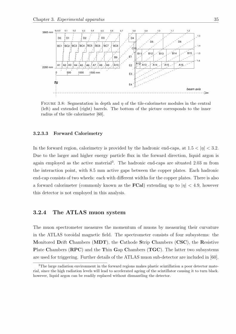
Chapter 3. Experimental apparatus 35
500 1000 1500 mm0
A3 A4 A5 A6 A7 A8 A9 A10A1 A2
BC1 BC2 BC3 BC5 BC6 BC7 BC8BC4
D0 D1 D2 D3
A13 A14 A15 A16
B9B12 B14 B15
D5 D6D4
C10
0,7 1,0 1,1
1,3
1,4
1,5
1,6
B11 B13
A12
E4
E3
E2
E1
beam axis
0,1 0,2 0,3 0,4 0,5 0,6 0,8 0,9 1,2
2280 mm
3865 mm =0,0η
~~
Figure 3.8: Segmentation in depth and η of the tile-calorimeter modules in the central(left) and extended (right) barrels. The bottom of the picture corresponds to the innerradius of the tile calorimeter [60].
3.2.3.3 Forward Calorimetry
In the forward region, calorimetry is provided by the hadronic end-caps, at 1.5 < |η| < 3.2.
Due to the larger and higher energy particle flux in the forward direction, liquid argon is
again employed as the active material3. The hadronic end-caps are situated 2.03 m from
the interaction point, with 8.5 mm active gaps between the copper plates. Each hadronic
end-cap consists of two wheels: each with different widths for the copper plates. There is also
a forward calorimeter (commonly known as the FCal) extending up to |η| < 4.9, however
this detector is not employed in this analysis.
3.2.4 The ATLAS muon system
The muon spectrometer measures the momentum of muons by measuring their curvature
in the ATLAS toroidal magnetic field. The spectrometer consists of four subsystems: the
Monitored Drift Chambers (MDT), the Cathode Strip Chambers (CSC), the Resistive
Plate Chambers (RPC) and the Thin Gap Chambers (TGC). The latter two subsystems
are used for triggering. Further details of the ATLAS muon sub-detector are included in [60].
3The large radiation environment in the forward regions makes plastic scintillation a poor detector mate-rial, since the high radiation levels will lead to accelerated ageing of the scintillator causing it to turn black.however, liquid argon can be readily replaced without dismantling the detector.
Chapter 3. Experimental apparatus 36
3.3 The ATLAS trigger system
With up to 1 GHz of data being delivered by the LHC during nominal running conditions, it
is impractical to store all of the detector information for every collision event. The multilevel
trigger system of ATLAS is designed to allow efficient identification and recording of ‘events
of interest’. For a full description of the ATLAS trigger system and its performance, see [62].
The identification of interesting events is based on the presence of one or more high transverse
momentum objects - for example a muon, electron, photon, jet, tau lepton or Missing
Transverse Energy (MET)4. These interesting events are characterised by sets of criteria
known as a trigger configuration (or trigger menu) which are composed of trigger chains.
Each one of these chains can be thought of as a logically independent set of criteria which
is either passed or failed by each event. For processes with high cross-sections, a trigger
prescale may be defined such that, for example, only 1 in 200 of events which satisfy that
trigger are recorded for further analysis. These prescales may be adjusted during data taking
in order to synchronise with the software model for offline processing and analysis.
ATLAS employs a three-level trigger system, with the rate of data recording being reduced
at each stage as a more stringent triggering criteria is applied. The Level 1 (L1) trigger is
hardware-based, using coarse detector information from the calorimeter, muon and forward
subsystems. The next two trigger levels are collectively known as the High Level Trigger
(HLT), and individually known as the Level 2 (L2) and Event Filter (EF). The HLT is
software-based with the EF running a physics reconstruction that is close to the offline
software. A schematic of the ATLAS trigger system, along with the nominal data-rates and
latencies5, is shown in Figure 3.9.
3.3.1 Triggering on jets
In this thesis, jet triggers are used to select events that contain a jet with high transverse
momentum. The inputs to the L1 jet trigger are the ∆η × ∆φ = 0.1 × 0.1 calorimeter
towers. A sliding window algorithm selects local maxima in transverse energy, ET . For a
4Assuming that the total linear momentum in the transverse plane of the detector is zero, the missingmomentum (or energy) is calculated from the vector sum of the momenta of all of the object coming fromthe primary vertex.
5Latency is how long the trigger hardware takes to reach a decision. In the case of the L1, the latencyis a strict limit of 2.5 µs, since this is the length of the data pipelines. In addition to latency, dead-time isa trigger veto that exists to stop the readout hardware being overwhelmed. Simple dead-time occurs whenthe L1 trigger accepts an event: the system will subsequently not accept any event from the next 5 bunchcrossings. The dead-time gives the readout system a breathing space of 125 ns to deal with the acceptedevent.
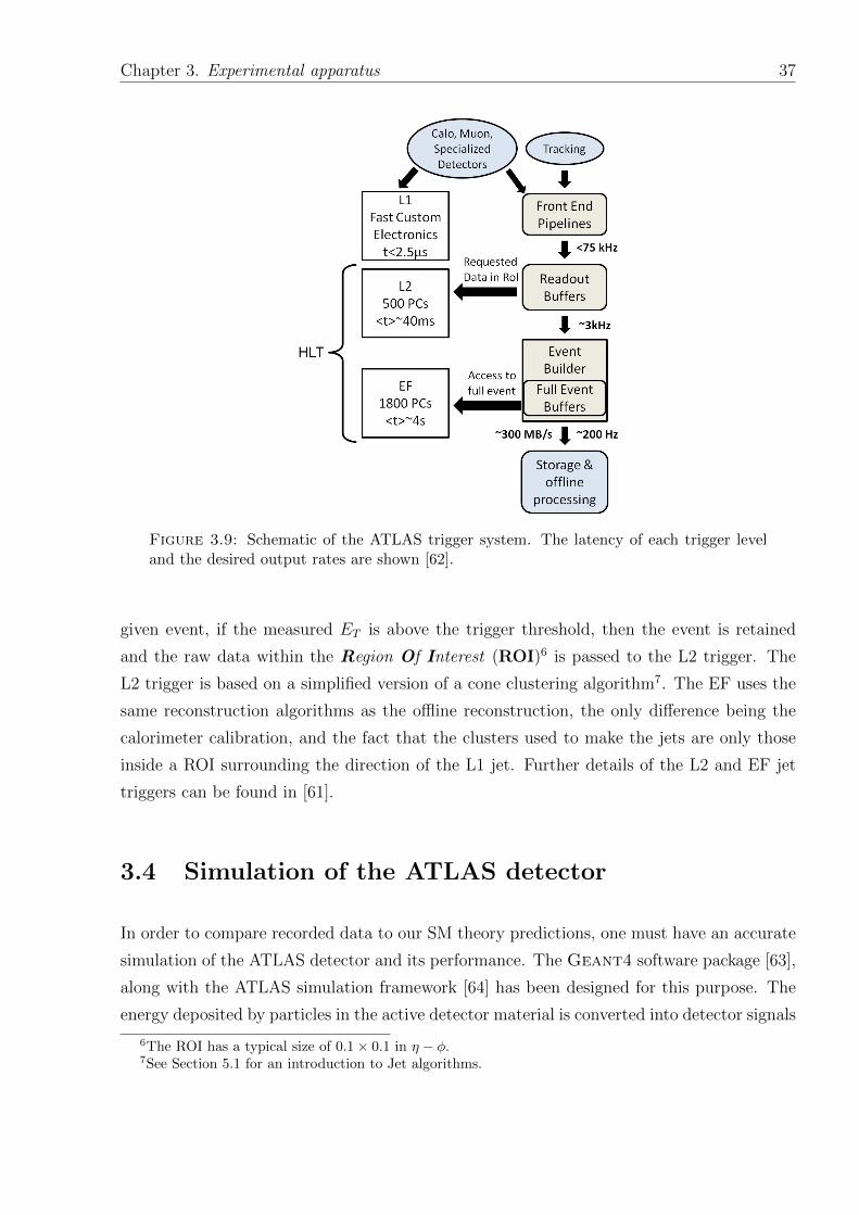
Chapter 3. Experimental apparatus 37
Figure 3.9: Schematic of the ATLAS trigger system. The latency of each trigger leveland the desired output rates are shown [62].
given event, if the measured ET is above the trigger threshold, then the event is retained
and the raw data within the Region Of Interest (ROI)6 is passed to the L2 trigger. The
L2 trigger is based on a simplified version of a cone clustering algorithm7. The EF uses the
same reconstruction algorithms as the offline reconstruction, the only difference being the
calorimeter calibration, and the fact that the clusters used to make the jets are only those
inside a ROI surrounding the direction of the L1 jet. Further details of the L2 and EF jet
triggers can be found in [61].
3.4 Simulation of the ATLAS detector
In order to compare recorded data to our SM theory predictions, one must have an accurate
simulation of the ATLAS detector and its performance. The Geant4 software package [63],
along with the ATLAS simulation framework [64] has been designed for this purpose. The
energy deposited by particles in the active detector material is converted into detector signals
6The ROI has a typical size of 0.1× 0.1 in η − φ.7See Section 5.1 for an introduction to Jet algorithms.
Chapter 3. Experimental apparatus 38
and reconstructed with the same format as the ATLAS detector read-out and online software.
The simulation is tuned by using data from test-beam and in-situ measurements.
The analysis presented in this thesis uses the ATLFAST II [65] package in order to provide
a faster and less CPU-intensive simulation of the ATLAS detector. ATLFAST II em-
ploys FastCaloSim [66] for the simulation of electromagnetic and hadronic showers in the
calorimeter. Careful comparisons with detailed simulations of the ATLAS detector [63, 64]
using the Geant4 package [63] show differences of the order of 1− 2%. A study performed
in the context of the dijet angular analysis is included in Appendix B.
3.5 Data used in this thesis
After a brief period of running at√s = 900 GeV, the LHC energy was increased to
√s =
2.36 TeV in late 2009. The machine energy was then ramped up to√s = 7 TeV - delivering
48.1 pb−1 of data in 2010 and 5.61 fb−1 of data in 2011.
The dataset analysed in this thesis corresponds to approximately 4.8 fb−1 recorded between
March and October of 2011. Although the LHC delivered 5.61 fb−1 of data in 2011, analysis
can only be performed on a subset of this data. This is mainly due to ATLAS being unavail-
able for short periods of time and also the time taken for ATLAS to begin recording data
once the LHC has achieved stable beams. The systematic error on the integrated luminosity
for the dataset considered in this thesis (this corresponds to data collected between March
and November of 2011) is 3.9% [59].
Figure 3.10 (a) shows the luminosity delivered and recorded by the LHC and ATLAS during
2011 proton-proton collisions. One can see the exponential increase in the instantaneous
luminosity, which occurs as a consequence of the continuous beam development.
A side effect of an increase in instantaneous luminosity is an increase in the number of
proton-proton interactions within the same bunch - know as in-time pile-up. It is also
possible to have multiple interactions from different bunches during the time taken for the
detector to process a single event - known as out-of-time pile-up. Out-of-time pile-up has
a further contribution from the circulation of multiple subsequent bunches in neighbouring
bunch-trains. The effects of pile-up are discussed further in Chapters 5 and 7.
The peak average number of proton interactions per bunch crossing is shown in Figure 3.10 (b).
As expected, the increase in the peak average is noticeably correlated to the instantaneous
luminosity (i.e. the gradient of the distribution in Figure 3.10 (a)).
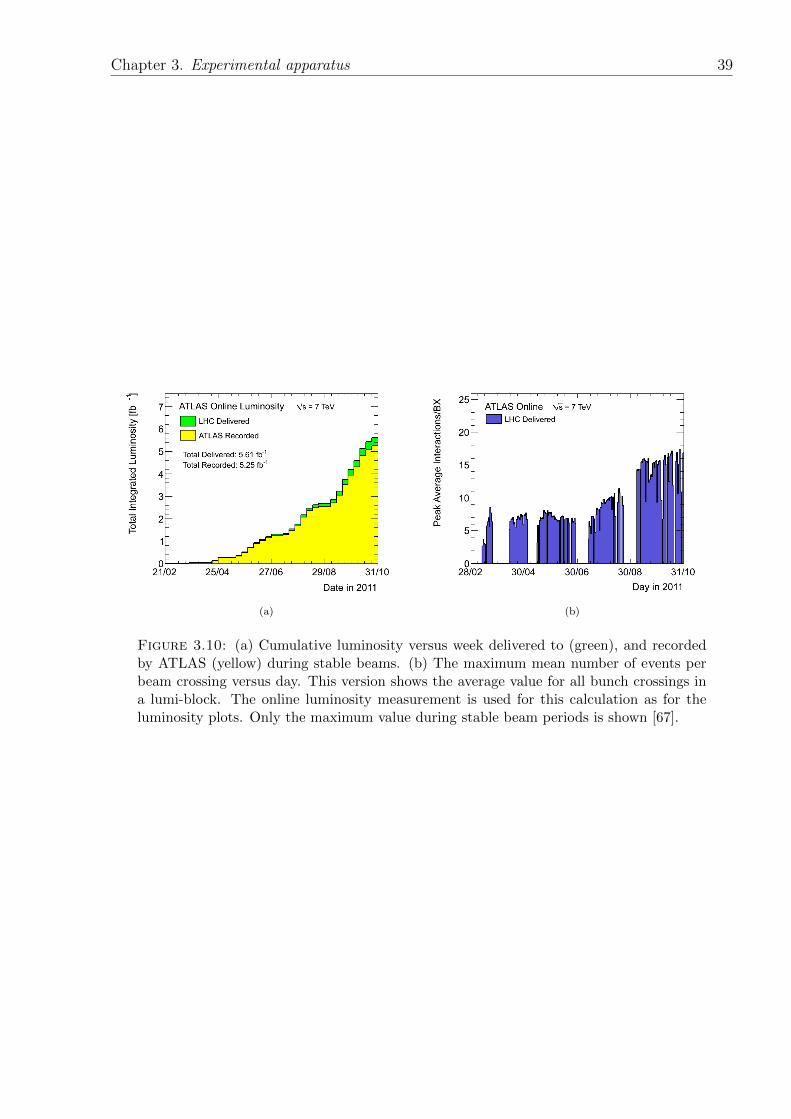
Chapter 3. Experimental apparatus 39
(a) (b)
Figure 3.10: (a) Cumulative luminosity versus week delivered to (green), and recordedby ATLAS (yellow) during stable beams. (b) The maximum mean number of events perbeam crossing versus day. This version shows the average value for all bunch crossings ina lumi-block. The online luminosity measurement is used for this calculation as for theluminosity plots. Only the maximum value during stable beam periods is shown [67].
Chapter 4
Beyond the standard model
Although the SM allows precise predictions for many processes: there is still room for many
alternative (and/or extended) theories to be correct. This chapter will introduce two scenar-
ios of beyond the standard model physics for which the analysis of this thesis is sensitive. The
scenarios are presented as effective theories with measurable deviation from the dominant
QCD cross-section and are considered as benchmark models: used to quantify the search
reach of a new physics analysis.
As well as being interesting examples of new physics scenarios, the three models are chosen
due to their fundamentally different final state phenomenology. Whilst the excited quark
model (Section 4.3.1) produces a resonance state, the quark contact interaction model (Sec-
tion 4.3.2) and Quantum Black Hole (Section 4.2) models are threshold processes with a slow
turn-on above a certain energy scale. In addition, whilst quantum black hole production is
independent of any other SM processes, the quark contact interaction model interferes with
the dominant QCD background.
4.1 Extra dimensions
Our every day experience is that of four dimensions - three of space and one of time. But
is it necessary that these are the only dimensions in our universe? Extra dimensions are
often postulated by theories which attempt to solve some of the biggest problems in theo-
retical physics, for example: the hierarchy problem, quantum gravity and unification of the
fundamental forces of nature.
40
Chapter 4. Beyond the standard model 41
Whilst General Relativity (GR) is one of the most successful and elegant theories in terms of
cosmological and astrophysical observations, its down fall occurs in the form of singularities
which occur at the high energies for which quantum effects become important. At the
other extreme, Quantum Mechanics (QM) impressively accounts for all known small scale
physics - however conceptual problems occur when it is applied to macroscopic systems. A
convolution of the two - a quantum theory of gravity is a holy grail of modern physics.
One belief is that the forces of the standard model, and perhaps also gravity, are in fact man-
ifestations of the same underlying force. This is known as unification. Some work towards
this goal has been achieved. Extra dimensions were first considered in connection to these
issues by the pioneering works of Kaluza [68] and Klein [69] in the 1920s. These works used
higher dimensional representations of the metric tensor in order to unify electromagnetism
with gravity.
The existence of > 3 spatial dimensions would have many interesting phenomenological
consequences, many of which, depending on the size and number of the ‘extra’ dimensions,
could be observable at the LHC.
If extra dimensions do exist, there must be some reason that we do not experience them in
our every day lives. Traditionally, this phenomenon is explained by supposing that any extra
dimensions are compactified on a small scale. Perhaps the two most popular configurations of
extra dimensions are the ADD (Arkani Hamed-Dimopoulos-Dvali) [70] and RS (Randall-
Sundrum) [71].
4.1.1 The Planck mass, MD
In the ADD [70] scenario of extra dimensions, space-time can be factorised into a 4-dimensional
part and a n-dimensional part (for n extra spatial dimensions). Following the PDG conven-
tion [8], the space is constructed as R4 ×Mn, where R4 is our usual 4-dimensional space-
time and Mn is a n−dimensional compact space with finite volume Vn. The factorisation
of the 4-dimensional and n−dimensional parts of the space-time allow one to express the
4-dimensional reduced Planck mass as
M2Pl = M2+n
D Vn, (4.1)
where MPl = MPl/√
8π = 2.4 × 10¹⁸ GeV and MD is the reduced Planck mass for the D-
dimensional theory. Following [72], the fundamental D−dimensional Planck mass is given
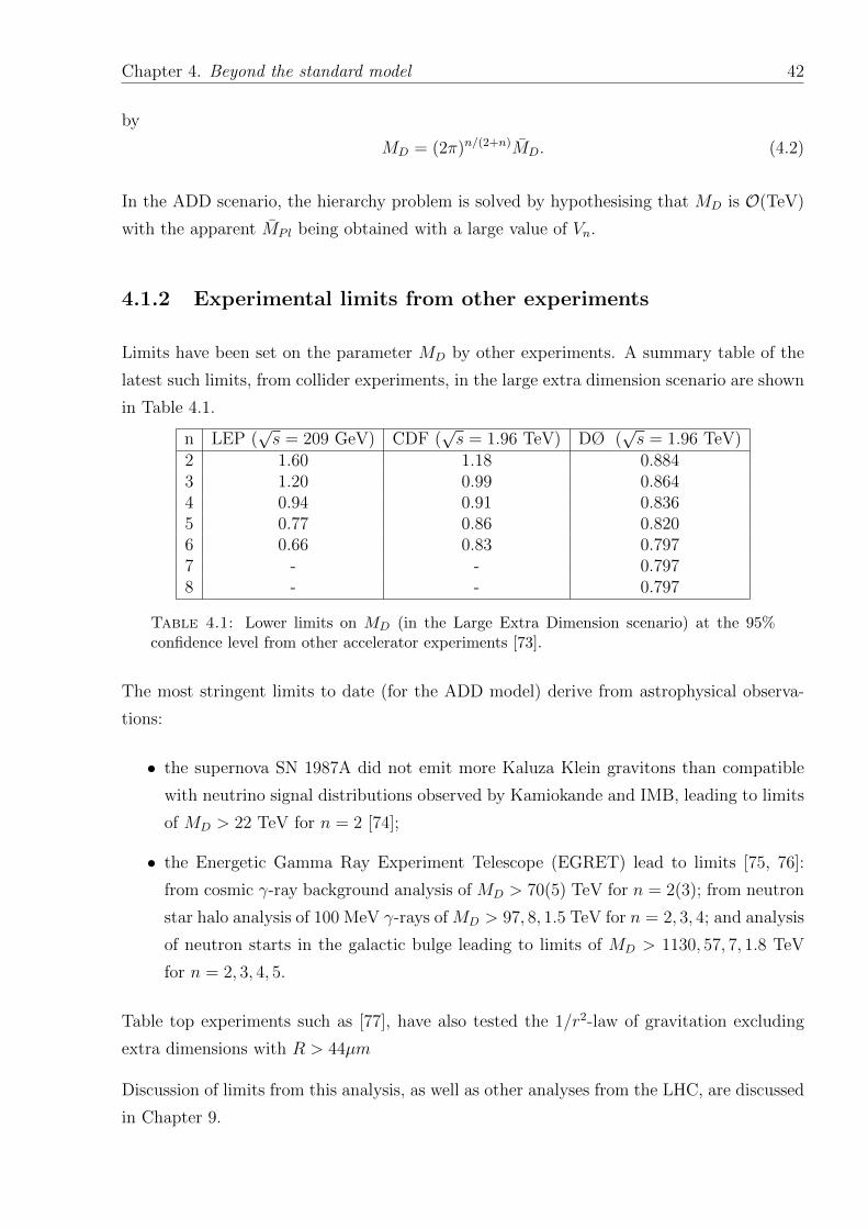
Chapter 4. Beyond the standard model 42
by
MD = (2π)n/(2+n)MD. (4.2)
In the ADD scenario, the hierarchy problem is solved by hypothesising that MD is O(TeV)
with the apparent MPl being obtained with a large value of Vn.
4.1.2 Experimental limits from other experiments
Limits have been set on the parameter MD by other experiments. A summary table of the
latest such limits, from collider experiments, in the large extra dimension scenario are shown
in Table 4.1.
n LEP (√s = 209 GeV) CDF (
√s = 1.96 TeV) DØ (
√s = 1.96 TeV)
2 1.60 1.18 0.8843 1.20 0.99 0.8644 0.94 0.91 0.8365 0.77 0.86 0.8206 0.66 0.83 0.7977 - - 0.7978 - - 0.797
Table 4.1: Lower limits on MD (in the Large Extra Dimension scenario) at the 95%confidence level from other accelerator experiments [73].
The most stringent limits to date (for the ADD model) derive from astrophysical observa-
tions:
• the supernova SN 1987A did not emit more Kaluza Klein gravitons than compatible
with neutrino signal distributions observed by Kamiokande and IMB, leading to limits
of MD > 22 TeV for n = 2 [74];
• the Energetic Gamma Ray Experiment Telescope (EGRET) lead to limits [75, 76]:
from cosmic γ-ray background analysis of MD > 70(5) TeV for n = 2(3); from neutron
star halo analysis of 100 MeV γ-rays of MD > 97, 8, 1.5 TeV for n = 2, 3, 4; and analysis
of neutron starts in the galactic bulge leading to limits of MD > 1130, 57, 7, 1.8 TeV
for n = 2, 3, 4, 5.
Table top experiments such as [77], have also tested the 1/r2-law of gravitation excluding
extra dimensions with R > 44µm
Discussion of limits from this analysis, as well as other analyses from the LHC, are discussed
in Chapter 9.
Chapter 4. Beyond the standard model 43
4.1.3 Warped extra dimensions
In the RS [71] model for extra-dimensions, the apparent weakness of gravity in our everyday
4-dimensional space-time is caused by a gravitational red-shift in a warped extra dimension.
The theoretical set-up consists of two 4-dimensional branes separated by a 5th y-coordinate.
The SM fields are located on the InfraRed (IR) brane and the other brane is known as the
UltraViolet (UV) brane. Solving Einstein’s equation given the element
ds2 = exp(−2k|y|)ηµνdxµdxν − dy2, (4.3)
with the UV and IR branes located at y = 0 and y = πR, respectively; R is the compactifica-
tion radius and k is the curvature of the extra dimension. In contrast to the ADD case, the
RS space is not factorised and so the 4-dimensional metric (and so the strength of gravity)
is dependent upon the extra-dimensional coordinate y.
4.1.4 Higgsless extra dimensional models
Although not of relevance to the particular models considered in this thesis, it is noted that
extra spatial dimensions also offer new possibilities for breaking gauge symmetries. Light
Kaluza-Klein modes on compactified spaces, corresponding to broken generators of the group,
acquire masses and allow the SM to respect unitarity up to E ∼ 12π2MW/g ∼ 10 TeV (for
a single extra dimension) [8].
4.1.5 Classical Black holes
The idea of a body so massive that even light could not escape was first put forward by
geologist John Michell in a letter written to Henry Cavendish in 1783.
Classically, in order for a particle of mass m to escape from the surface of a planet or star
of mass M :1
2mv2 >
GMm
r, (4.4)
where G is the gravitational constant and r is the radius of the planet or star. Therefore, in
the limit that the escape velocity is equal to the speed of light, c, then
r = rS =2GM
c2, (4.5)
Chapter 4. Beyond the standard model 44
where rS is known as the Schwarzschild radius: a particle that is at a distance d < rS from
the centre of mass will require a speed > c in order to escape the gravitational attraction of
the body. The sphere about the centre-of-mass of M with radius rS is known as the event
horizon: due to the universal speed limit of any object being c [78], any event within the
event horizon can have no causal effect beyond the event horizon.
For ordinary stars and planets r > rS. For example, our sun has r = 700, 000 km with
rS = 3 km. However, as explained above, for r < rS, we have a situation where an object
would require a speed > c in order to escape the star: a black hole is formed.
Later, solutions to Einstein’s equations were found for rotating, charged and charged rotating
Black Holes (BHs) eventually leading to the no-hair theorem stating that a stationary black
hole solution is completely described by the three parameters of the Kerr-Newman metric:
mass, angular momentum and electric charge.
4.1.6 Higher dimensional Black Holes
In the absence of extra dimensions, the creation of a BH requires extremely large CM energies:
reducing the CM energy down to energy scales accessible at the LHC leads to a Schwarzschild
radius, which is so small that a BH can not be formed.
For a universe with extra dimensions, if the Compton wavelength of a given mass is much
larger than the size of the extra dimensions, then the mass will behave as a 4-dimensional
object: this is the situation for regular objects such as people, planets and classical black
holes. If, however, the Compton wavelength of an object is smaller than the size of the extra
dimensions, then the object exists as a higher-dimensional object that is completely sub-
merged in a higher dimensional space-time. The presence of the extra dimensions facilitates
the creation of BH, since, for a higher dimensional object, the scale of gravity is increased:
increasing the corresponding Schwarzschild radius for a given mass.
By lowering Plank scale MD closer to the EW scale, the possibility of BH production in high-
energy scattering processes becomes a possibility for reactions with trans-Plankian centre-
of-mass energies,√s > MD. For a centre-of-mass energy
√s with D = 4 + n space-time
dimensions, the Schwarzschild radius is given by [79]
rS = k(D)1
MD
(M
MD
) 1D−3
, (4.6)
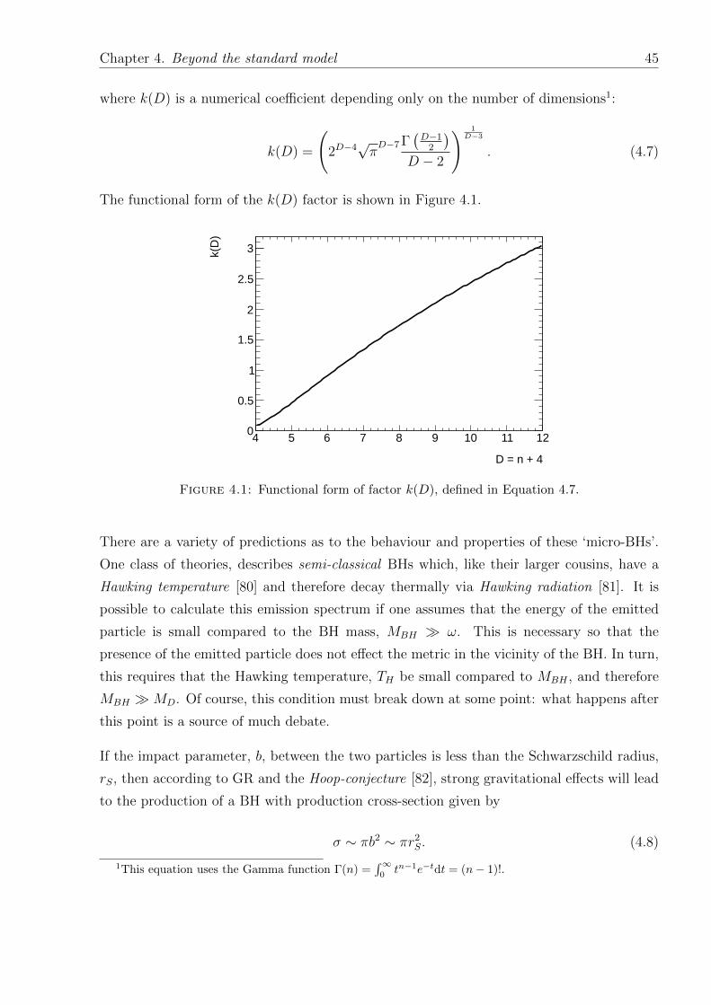
Chapter 4. Beyond the standard model 45
where k(D) is a numerical coefficient depending only on the number of dimensions1:
k(D) =
(2D−4
√πD−7 Γ
(D−1
2
)D − 2
) 1D−3
. (4.7)
The functional form of the k(D) factor is shown in Figure 4.1.
D = n + 4
4 5 6 7 8 9 10 11 12
k(D
)
0
0.5
1
1.5
2
2.5
3
Figure 4.1: Functional form of factor k(D), defined in Equation 4.7.
There are a variety of predictions as to the behaviour and properties of these ‘micro-BHs’.
One class of theories, describes semi-classical BHs which, like their larger cousins, have a
Hawking temperature [80] and therefore decay thermally via Hawking radiation [81]. It is
possible to calculate this emission spectrum if one assumes that the energy of the emitted
particle is small compared to the BH mass, MBH ω. This is necessary so that the
presence of the emitted particle does not effect the metric in the vicinity of the BH. In turn,
this requires that the Hawking temperature, TH be small compared to MBH , and therefore
MBH MD. Of course, this condition must break down at some point: what happens after
this point is a source of much debate.
If the impact parameter, b, between the two particles is less than the Schwarzschild radius,
rS, then according to GR and the Hoop-conjecture [82], strong gravitational effects will lead
to the production of a BH with production cross-section given by
σ ∼ πb2 ∼ πr2S. (4.8)
1This equation uses the Gamma function Γ(n) =∫∞0tn−1e−tdt = (n− 1)!.
Chapter 4. Beyond the standard model 46
During this process, not all of the incident energy of the two particles is bound to the BH.
A fraction of the energy will be lost through gravitational radiation.
In a scenario with extra dimensions, the trans-Plankian regime may lie slightly above the
TeV scale. In this case, it is entirely possible trans-Plankian reactions already take place in
the atmosphere [83–86]. In this thesis, the possibility of these reactions taking place under
the controlled conditions of the LHC is considered.
4.2 Quantum Black Holes
In [87–90] it is argued that the semi-classical black holes (described above) are highly sup-
pressed and will in-fact occur in only a very limited parameter range of the models, if at all.
In addition, the expected number of particles to be emitted from the BH is only above 2 for
MBH ≥ 1.5MD. The steeply falling parton distributions functions of the proton lead to a
cross-section for BH production that is strongly peaked at their production threshold, which
is assumed to be MD. As alluded to above, the behaviour of particle interactions around the
Planck scale is shrouded by a lack of knowledge of quantum gravity. It is therefore perhaps
more appropriate to refer to such an interaction of a ‘quantum gravitational effect’ or ‘res-
onance’, however we follow the common convention of referring to such states as Quantum
Black Holes (QBH).
Despite the absence of a complete quantum theory of gravity, by making a few assumptions
and relying on fundamental principals [91], it is possible to construct a model for production
and decay of QBHs in proton proton collisions at the LHC [79].
4.2.1 Quantum black hole production at the LHC
For a proton-proton (pp) collision, following the arguments outlined above, it is required
that any two partons (i, j) have an impact parameter b < bc ' rS, where bc is the critical
value and rS is given in Equation 4.6. The parton-level production cross-section is simply
σij ' πr2S(s), where
√s is the centre-of-mass energy of the colliding partons. In order to
construct the complete cross-section, we must sum over all possible parton combinations, and
weight them according to the parton distribution functions fi(x), which give the probability
of finding a parton of flavour i, with momentum fraction x of the colliding proton. The total
pp cross-section for the production of a BH from the collision of two partons, a and b, may
Chapter 4. Beyond the standard model 47
be written as
σ(QBHqp1p2
) =∑a,b
∫ 1
M2/s
dxmin
∫ 1
xmin
dx
xfa
(xminx
)fb(x)πr2
S, (4.9)
where sxaxb = sxmin = s (xa and xb are the fractional energies of the two partons relative
to the proton energies), and fa and fb are the PDFs for the proton. The naming convention
for QBH states used in [79] has been adopted in this thesis such that the state QBHqp1p2
is
formed from parton types p1 and p2 and has electric charge q. Since it is natural for local
gauge symmetries of QCD colour and electric charge to be conserved during the black hole
formation [90], the possible decay states of the QBH are determined by q and the colour
state composed from p1 and p2. It should be remembered that this production cross-section
is, most likely, an over-estimation, since we have assumed bc ' rS and that all of the energy
goes into the creation of the BH. As discussed above, it more likely that bc < rS and that a
significant fraction of the CM energy is lost through gravitational radiation effects.
4.2.2 Simulation with the BlackMax generator
QBH simulations are produced using the BlackMax V2.0 Monte Carlo generator [92, 93].
BlackMax is a versatile semi-classical and quantum black-hole generator that simulates
a number of different extra dimension models and black-hole evolution scenarios. In this
thesis, a QBH model resulting in two final-state particles is simulated. A basic model is
chosen for QBH states to be produced for MD ≤√s ≤ √s, where 100% of the combined
partonic energy is included in the QBH production2. The production and decay of the QBH
is simulated as an s-channel process with an isotropic decay distribution in the final state. In
the decay of the QBH states, it is required that baryon number be conserved. The resulting
branching ratios to SM particles for the case of MD = 4 TeV and n = 6 are shown in
Table 4.2 - the total branching ratio for dijet final states is 96.32%.
The production cross-section for n = 6 extra dimensions and values of MD ranging from
2 TeV to 5 TeV are given in Table 4.3. For limit setting purposes, 10,000 events of each
mass-point for the n = 6 scenario were simulated and passed through the ATLAS simulation
chain described in Section 2.4.
As the value of MD increases, so does the energy threshold for the production of QBH states:
resulting in a lower production cross-section. The variation of the production cross-section
with n can be understood through Equation 4.7 and Figure 4.1.
2The parameter file for the particular model is included in Appendix E of this thesis.
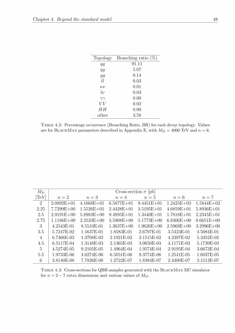
Chapter 4. Beyond the standard model 48
Topology Branching ratio (%)qq 91.11qg 5.07gg 0.14ll 0.03νν 0.01lν 0.03γγ 0.00V V 0.02HH 0.00other 3.58
Table 4.2: Percentage occurrence (Branching Ratio, BR) for each decay topology. Valuesare for BlackMax parameters described in Appendix E, with MD = 4000 TeV and n = 6.
MD Cross-section σ [pb][TeV] n = 2 n = 3 n = 4 n = 5 n = 6 n = 7
2 2.0892E+01 4.1668E+01 6.5877E+01 9.4451E+01 1.2425E+02 1.5844E+022.25 7.7299E+00 1.5526E+01 2.4428E+01 3.5195E+01 4.6859E+01 5.8936E+012.5 2.9191E+00 5.8983E+00 9.4895E+01 1.3440E+01 1.7818E+01 2.2345E+012.75 1.1186E+00 2.2533E+00 3.5908E+00 5.1773E+00 6.8306E+00 8.6651E+00
3 4.2543E-01 8.5510E-01 1.3637E+00 1.9626E+00 2.5969E+00 3.2996E+003.5 5.7247E-02 1.1637E-01 1.8583E-01 2.6797E-01 3.5423E-01 4.5084E-014 6.7466E-03 1.3708E-02 2.1921E-02 3.1515E-02 4.2397E-02 5.3352E-02
4.5 6.5117E-04 1.3148E-03 2.1365E-03 3.0650E-03 4.1171E-03 5.1739E-035 4.5274E-05 9.2105E-05 1.4964E-04 1.9574E-04 2.9195E-04 3.6673E-04
5.5 1.9733E-06 4.0274E-06 6.5051E-06 9.3774E-06 1.2541E-05 1.6037E-056 3.8140E-08 7.7826E-08 1.2722E-07 1.8384E-07 2.4380E-07 3.1513E-07
Table 4.3: Cross-sections for QBH samples generated with the BlackMax MC simulatorfor n = 2− 7 extra dimensions and various values of MD.
Chapter 4. Beyond the standard model 49
4.3 Quark sub-structure
The SM does not predict the masses of fermions or their family structure described in
Section 1.2. In addition, the SM does not motivate the relationship between the charges
of elementary particles. This situation allows a hint for the possibility of fermions being
composite objects.
It is hypothesised that if quarks and leptons consist of bound constituents (often named
preons) then new interactions will be measurable at some energy scale Λ, known as the
composite scale. In the following sections, two effective models of quark sub-structure are
described. These models provide a popular benchmark scenario for NP searches among high-
energy collider experiments: allowing simplified comparison between the performance and
methods of different collaborations.
4.3.1 Excited quarks
The excited quark model [94–96] is one implementation of a theory with quark sub-structure
and is a commonly used benchmark signal in high-energy experiment searches: used to
quantify the search reach of an analysis. Quarks consisting of tightly bound elementary
constituents are energised to excited states and then subsequently decay in an s-channel
process. If the energy scale at which compositeness effects are relevant, Λ, is smaller than
the centre-of-mass energy of the LHC then it is expected that such quark resonances will be
visible.
Taking the first generation of excited quarks, denoted as q∗ (u∗, d∗), are assumed to have
spin and isospin equal to 1/2 with their couplings to SM quarks and gauge bosons dictated
by the Lagrangian [96]:
Lq∗ =1
2Λq∗Rσ
µν
[gsfs
λa
2Gaµν + gf
τ
2Wµν + g′f ′
Y
2Bµν
]qL + h.c. (4.10)
where Gaµν , Wµν and Bµν are the field-strength tensors of the SU(3), SU(2) and U(1) gauge
fields, respectively. The quantities λa, τ and Y (gs, g and g′) and the corresponding gauge
structure constants (gauge coupling constants). The parameters fs, f and f ′ control the
composite dynamics and are expected to be of order one. For mq∗ > mV (V = W±, Z0) and
Chapter 4. Beyond the standard model 50
1 TeV 2 TeV 3 TeV 1 TeV 2 TeV 3 TeVBR(u∗ → ug) 82.7% 81.4% 80.7% BR(d∗ → dg) 82.7% 81.4% 80.7%BR(u∗ → uγ) 2.4% 2.5% 2.6% BR(d∗ → dγ) 0.6% 0.6% 0.7%BR(u∗ → uZ0) 3.5% 3.8% 4.0% BR(d∗ → dZ0) 5.3% 5.7% 5.9%BR(u∗ → uW−) 11.4% 12.3% 12.8% BR(d∗ → dW+) 11.4% 12.3% 12.8%
Γ(u∗)/mu∗ 0.0374 0.0352 0.0341 Γ(d∗)/md∗ 0.0374 0.0352 0.0341
Table 4.4: Branching ratios and relative decay widths for q∗ (mq∗ = 1, 2, 3 TeV) to variousdecay channels. Using ATLAS MC09 tuning [99] and taken from [100].
massless ground-state quarks, the partial widths [96–98] for the q∗ decays are
Γ(q∗ → qg) =1
3αSf
2S
m3q∗
Λ2, (4.11)
Γ(q∗ → qγ) =1
4αf 2
γ
m3q∗
Λ2,
Γ(q∗ → qV ) =1
8
g2V
4πf 2V
m3q∗
Λ2
(1− m2
V
m2q∗
)2(2 +
m2V
m2q∗
),
with
fγ = fT3 + f ′Y
2, (4.12)
fZ = fT3 cos2 θW − f ′Y
2sin2 θW ,
fW =f√2,
where T3 is the third component of weak isospin and Y is the hypercharge of q∗.
A compositeness scale Λ = mq∗ and SM couplings (fS = f = f ′ = 1) results in the branching
ratios given in Table 4.4. With a coupling strength of m2jj/Λ
2 ∼ O(1), the excited quark
production has a coupling greater than 2 orders of magnitude above αS. Consequently,
any interference terms between the excited quark Lagrangian (Equation 4.10) and SM QCD
processes can be neglected. Distributions of the excited quark signal for the observables used
in this thesis are shown in Sections 8.2.2 and 8.2.3.
This excited quark model is available in the Pythia 6 [50] event generator, and has been
used as a benchmark to set limits on q∗ in ATLAS, in CMS, and in TeVatron experiments.
An example of the kinematic distributions for an excited quark with a mass of 1 TeV is
shown in Figure 6.7. Unfortunately, in the course of preparing for analysis of ATLAS 2012
collision data it has been found that there is a problem with this benchmark. In 2012,
ATLAS is using the C++ based Pythia 8 [101] event generator for processes previously
simulated with Pythia 6 since the older generator will no longer be supported by its authors.
Chapter 4. Beyond the standard model 51
[GeV]jjm
1000 1500 2000 2500 3000 3500 4000 4500
(pb/G
eV
)jj
/dm
σd
0
0.0005
0.001
0.0015
0.002
0.0025
0.003
0.0035 Original Q*
Fixed Q*
= 3 TeV*q
< 0.6, m*
y
Figure 4.2: Comparison of the q∗ mjj distribtions from Pythia 6 with and without theFSR correction, for a q∗ mass of 3 TeV.
In anticipation of this change, a number of studies have been done in ATLAS comparing
standard model and NP processes with these two generators. The q∗ comparison studies
show that there are noticeable differences in the dijet mass distributions predicted by the
two generators. In particular, the Pythia 8 dijet mass peak for q∗ is substantially wider
than that for Pythia 6.
The Pythia authors confirm that there is a problem with the showers in Pythia 6 for the
excited quark model: the generator gives too little final state radiation (FSR). The problem
lies with the matrix-element (ME) correction machinery, which is intended to ensure that
the showers are correct to NLO. Pythia 6 handles the FSR correctly for SM and MSSM
processes but in the case of q∗, and some other processes, it rejects most radiation associated
with one of the jets. In Pythia 8, the list of matrix elements is the same, but the process
identification is more sophisticated, and the colour flow is handled correctly.
The q∗ mjj distributions from Pythia 6 can be brought into close correspondence with
Pythia 8 by setting the Pythia 6 MSTJ(47) parameter to zero, approximating the correct
process identification and restoring the FSR.
Since Pythia 6 with the default setting has been used by a number of experiments to set
q∗ limits, it has been decided to create two sets of MC samples, with and without the FSR
modification, and to calculate the q∗ exclusion limits for both cases. A comparison of the
signal shapes for an excited quark of mass 3 TeV is shown in Figure 4.2.
The corresponding cross-sections and number of events for the excited quark samples gen-
erated with Pythia 8 are shown in Table 4.5.
Chapter 4. Beyond the standard model 52
mq∗ [GeV] cross-section sigma [pb] Nevents generated2000 1.5721 200002250 0.54626 200002500 0.19819 200002750 0.071970 200003000 0.026747 200003250 0.010041 200003500 0.0039463 200003750 0.0015547 200004000 0.000639 200004250 0.00028174 200004500 0.00013449 20000
Table 4.5: Cross-section and number of events generated for Pythia 8 excited quark atq∗ masses from 2 to 4.5 TeV.
The best non-LHC exclusion limits, to-date, on the mass of the q∗ were set by CDF Run 2
at the Tevatron and excluded the mass region 260 < mq∗ < 870 GeV [102].
4.3.2 Quark contact interactions
In contrast to the tightly bound constituents of the excited quark model in Section 4.3.1, it
is often postulated that partons may simply be unstructured collections of preons [103–105].
Of particular interest, is the possibility of a four point ‘Contact Interaction’ (CI). For a
2 → 2 process, we have the possibility of two energy regimes depicted in Figure 4.3. For
M Λ the interaction is dominated by classical QCD. However, for energies at and beyond
Λ, the interaction can be described by the effective Lagrangian:
LΛ =g2
2Λ2[ηLL(qLγ
µqL)(qLγµqL) + ηRR(qRγµqR)(qRγµqR) + 2ηRL(qRγ
µqR)(qLγµqL)] , (4.13)
where the coefficients ηab can be set to 0, +1 or −1 in order to turn terms on/off or select
constructive/destructive interference.
In this thesis, the common convention of left-left isoscalar destructive interference is employed
as a specific example as an alternative to the QCD null hypothesis. The resulting Lagrangian
is
LΛLL =4π
2Λ2(qLγ
µqL)(qLγµqL). (4.14)
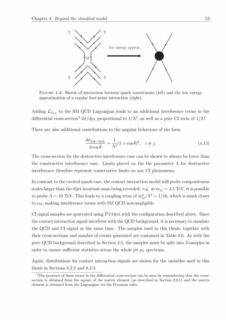
Chapter 4. Beyond the standard model 53
M
q
q
q
q
low energy approx.
Figure 4.3: Sketch of interaction between quark constituents (left) and the low energyapproximation of a regular four-point interaction (right).
Adding LΛLL to the SM QCD Lagrangian leads to an additional interference terms in the
differential cross-section3 dσ/dpT proportional to 1/Λ2, as well as a pure CI term of 1/Λ4.
There are also additional contributions to the angular behaviour of the form
dσqiqi→qj qj
d cos θ∼ 1
Λ4(1 + cos θ)2, i 6= j. (4.15)
The cross-section for the destructive interference case can be shown to always be lower than
the constructive interference case. Limits placed on the the parameter Λ for destructive
interference therefore represent conservative limits on any CI phenomena.
In contrast to the excited quark case, the contact interaction model will probe compositeness
scales larger than the dijet invariant mass being recorded: e.g. atmjj ∼ 2.5 TeV, it is possible
to probe Λ ∼ 10 TeV. This leads to a coupling term of m2jj/Λ
2 ∼ 1/16, which is much closer
to αS, making interference terms with SM QCD non-negligible.
CI signal samples are generated using Pythia with the configuration described above. Since
the contact interaction signal interferes with the QCD background, it is necessary to simulate
the QCD and CI signal at the same time. The samples used in this thesis, together with
their cross-sections and number of events generated are contained in Table 4.6. As with the
pure QCD background described in Section 2.5, the samples must be split into J-samples in
order to ensure sufficient statistics across the whole jet pT spectrum.
Again, distributions for contact interaction signals are shown for the variables used in this
thesis in Sections 8.2.2 and 8.2.3.
3The presence of these terms in the differential cross-section can be seen by remembering that the cross-section is obtained from the square of the matrix element (as described in Section 2.2.1) and the matrixelement is obtained from the Lagrangian via the Feynman rules.
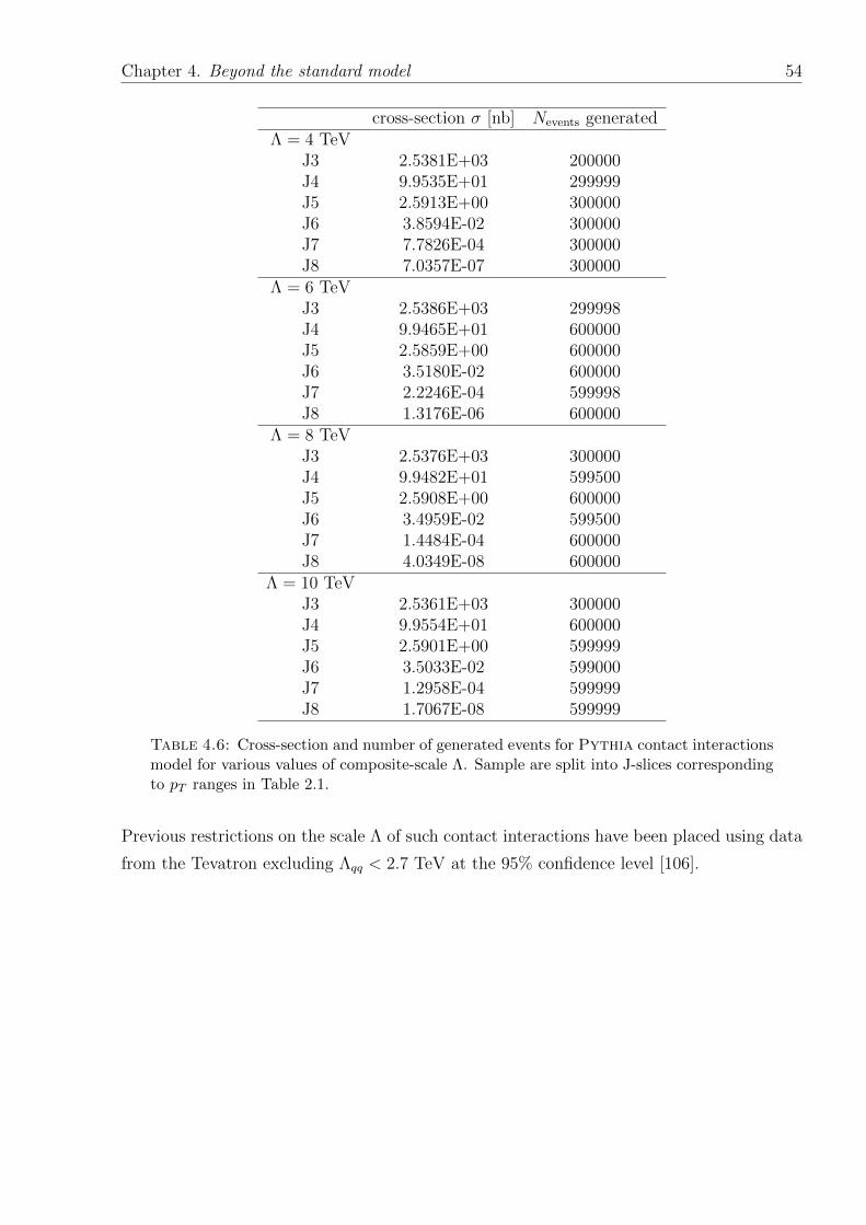
Chapter 4. Beyond the standard model 54
cross-section σ [nb] Nevents generatedΛ = 4 TeV
J3 2.5381E+03 200000J4 9.9535E+01 299999J5 2.5913E+00 300000J6 3.8594E-02 300000J7 7.7826E-04 300000J8 7.0357E-07 300000
Λ = 6 TeVJ3 2.5386E+03 299998J4 9.9465E+01 600000J5 2.5859E+00 600000J6 3.5180E-02 600000J7 2.2246E-04 599998J8 1.3176E-06 600000
Λ = 8 TeVJ3 2.5376E+03 300000J4 9.9482E+01 599500J5 2.5908E+00 600000J6 3.4959E-02 599500J7 1.4484E-04 600000J8 4.0349E-08 600000
Λ = 10 TeVJ3 2.5361E+03 300000J4 9.9554E+01 600000J5 2.5901E+00 599999J6 3.5033E-02 599000J7 1.2958E-04 599999J8 1.7067E-08 599999
Table 4.6: Cross-section and number of generated events for Pythia contact interactionsmodel for various values of composite-scale Λ. Sample are split into J-slices correspondingto pT ranges in Table 2.1.
Previous restrictions on the scale Λ of such contact interactions have been placed using data
from the Tevatron excluding Λqq < 2.7 TeV at the 95% confidence level [106].
Chapter 5
Jet reconstruction
A jet is a narrow cone of hadrons and other particles produced by the hadronisation of a
quark or gluon. Within the ATLAS detector, many, if not most, interesting final states will
include at least one jet in the final state.
The expected behaviour of final state partons was discussed in Chapter 2. This discussion
described proton collisions resulting in final state hadrons, together with a cross-section for
that process. This chapter will look at these processes from the other direction: starting
with energy depositions in the ATLAS calorimetry from highly energetic hadrons, we shall
describe the procedure required to extract a measurement of the process at the particle level.
The ultimate goal is to be able to compare theoretical predictions, introduced in Section 2.3,
with experimental measurements.
5.1 Motivations for jet definitions
Since we are unable to observe the final-state partons of a hard scatter in a proton-proton
collision, a common prescription must be defined for accurate comparison of jets from theory
and experimentally measured jets. This prescription must describe how to uniquely map a
set of four-momenta (whether particles, partons or calorimeter objects) into a jet object.
Following the convention of 2007 Les Houches accord [107], a complete jet definition must
include:
• a jet algorithm that defines how to group four-momenta of particles, partons or
calorimeter objects into jets;
55
Chapter 5. Jet reconstruction 56
• the full specification of the jet algorithm parameters;
• the recombination scheme: a set of rules for obtaining the four-momentum of the
final jet object from its constituents.
The development of a jet definition must take into account both theoretical and experimental
considerations. Some of these factors will be discussed below, however a more complete
description is given in [108].
As described in Chapter 2, the scaling of the strong coupling constant leads to distinct
energy regimes where perturbative QCD methods may or may not be employed. These
issues can lead to apparent singularities in the cross-sections associated with infra-red and
collinear emissions of quarks and gluons. The jet definition must be resilient to the pres-
ence (or absence) of these low-energy emissions. Theoretically, well-behaved jets give finite
perturbative results at all orders and allow meaningful comparisons of data with the most
recent theoretical predictions. A jet definition that is insensitive to the presence of additional
very soft particle radiation1 is known as infra-red-safe. A jet definition that is insensitive to
the presence of additional particles radiated at a very small angle, with respect the original
parton, is known as collinear safe.
It is also required that the jet definition is able to reproduce the same physics results:
whether the input objects are particles, partons or calorimeter objects - in other words,
the jet definition should be detector-independent. Furthermore, it is desirable that the
jet algorithm is invariant under longitudinal boosts along the beam axis: therefore aiding
comparison between the lab and the CM frame.
Experimental considerations include the implementation and speed of the jet algorithm,
as well as its resilience toward calorimeter noise, pile-up conditions and the calibration
scheme. For the ATLAS experiment, the jet reconstruction software is implemented through
the ATHENA software framework, which employs the FastJet [109, 110] classes for jet
finding. Detector and calibration effects for some jet algorithms are discussed below.
5.2 Jet finding algorithms in ATLAS
There are two broad collections of jet algorithms: those based on geometrical cones in
(η, φ); and those that involve repeated recombination of constituent particles, based on some
1i.e. In the limit of increasingly low momentum particle radiation
Chapter 5. Jet reconstruction 57
predefined distance parameter. Each approach has relative theoretical and experimental
strengths and so are employed in different areas of an ATLAS analysis.
5.2.1 The cone algorithm
The seeded fixed cone algorithm starts with ordering the inputs according to decreasing
transverse momentum, pT . The highest pT object is selected if it satisfies a seed thresh-
old of 1 GeV. Subsequently, all objects within a cone of fixed-radius Rcone in (η, φ) are
combined with the seed. The four-momenta of the grouped objects are added to form the
four-momentum of a secondary seed around which a new cone is formed. Objects are then
(re-)collected in this new cone. The process continues until the direction of the collected
cone is stable, i.e. does not change significantly during successive iterations - resulting in a
final jet object. This process then begins again taking the next-highest pT seed.
The final collection of jets may share constituents, therefore a split and merge step is included:
jets that share more than a fraction fsm (fsm = 0.5 in ATLAS) of the pT of the jets are
merged, otherwise they are split.
The seeded cone algorithm is collinear but not infra-red safe: i.e. soft particles can easily
modify its behaviour. However, due to its speed, the seeded cone algorithm is used in order
to quickly form jet objects within the ATLAS jet trigger software: see Section 3.3.1.
5.2.2 The anti-kT algorithm
The anti-kT jet algorithm is an example of a sequential recombination algorithm and is the
default ATLAS jet algorithm. For this algorithm, all pairs (i, j) of input objects are analysed
with respect to their relative distance measures:
dij = min
(1
p2T,i
,1
p2T,j
)∆R2
ij
R2= min
(1
p2T,i
,1
p2T,j
)∆η2
ij + ∆φ2ij
R2(5.1)
and diB = 1/p2T,i, where the index B stands for Beam and R is a pre-defined cone size
parameter (for which we use R = 0.6). The algorithm then progresses as:
• The minimum distance dmin among dij and diB is found.
• If dmin corresponds to value from the list of dij: the objects i and j are combined into
a new object k.
Chapter 5. Jet reconstruction 58
• Elements i and j are removed from the list of input objects and k is added to the list.
• If dmin corresponds to a value from the list of diB: object i is considered a jet and is
removed from the list.
• The procedure is repeated until all objects are removed from the list.
The anti-kT algorithm is both infra-red and collinear safe and requires no split and merge
stage.
After a detailed study of jet algorithms within ATLAS [111] (considering cone sizes of 0.4 and
0.7) it was decided that the anti-kT algorithm demonstrated the best overall performance -
and so was adopted as the default algorithm for offline reconstruction. It was found that the
anti-kT algorithm is stable against pile-up, due to the fact that it is infra-red and collinear
safe. However, since the algorithm does not use a seed, it is more sensitive to electronic
noise in the calorimeter. As a result of this, the algorithm is used with input objects that
are noise suppressed - see Section 5.3.
It was also found that the ATLAS trigger efficiency would improve through the use of anti-
kT , however for the measurement described in this thesis, this has not-yet been implemented
and the trigger uses the cone algorithm.
5.3 Jet reconstruction in ATLAS
For the ATLAS experiment, jets can be reconstructed from different physics objects. In
this thesis, topological clusters, or topoclusters [112] are used as an input to the anti-kT jet
algorithm with R = 0.6. Alternative input objects are: groups of geometrically delimited
groups of calorimeter cells, known as towers ; and reconstructed tracks, resulting in track
jets. Truth jets are also used in some studies, which are reconstructed from stable2 particles
generated by the Monte Carlo event generator. For a more complete description of the
behaviour of jets in ATLAS, see [113].
Topological clusters are groups of calorimeter cells that are designed to follow the shower
development, whilst taking advantage of the fine segmentation of the ATLAS calorimeters.
Starting with a seed cell, whose signal-to-noise ratio3 is above a threshold of 4, neighbouring
cells are included iteratively if their signal-to-noise ratio is ≥ 2, and then all neighbouring
2A stable particle is defined to have a lifetime > 10 ps.3The signal-to-noise ratio is estimated as the energy deposited in the calorimeter cell divided by the RMS
of the energy distributions measured in randomly triggered events.
Chapter 5. Jet reconstruction 59
cells are also also included. Once all prospective cells have been added together, all cells in a
topocluster are scanned for local maxima in terms of energy content. Any local maxima are
then used as seeds for a new iteration for topological clustering, which will split the original
cluster into more topoclusters.
Four-vectors for the final topoclusters are constructed with energy equal to the sum of
the energy of the included cells, zero mass and a reconstructed direction as that of a unit
vector originating from the centre of the ATLAS coordinate system and pointing to the
energy-weighted topocluster barycentre. The process for calibrating the energy of each of
the topoclusters, as well as moving the direction of each topocluster to the primary vertex,
is described in Section 5.4.
5.4 Jet energy scale & calibration
As described in Section 3.2.3, the ATLAS calorimeters are non-compensating. Starting
with energy deposits that have been calibrated at the electromagnetic scale, it is therefore
necessary to re-scale the energy of topoclusters to account for the lower hadronic response.
This Section will provide a basic description of the method used to calculate this Jet Energy
Scale (JES). The uncertainty on this knowledge is the major contributor to the systematic
uncertainty of the final observables of this thesis: details associated with the derivation,
application and uncertainty associated with the JES are discussed.
As a starting point, the energy deposits within individual readout cells are recorded at the
ElectroMagnetic (EM) scale. The EM scale calibration and its uncertainty are derived from
a combination of techniques, including: comparison of electronic pulse signal shapes4, and
measurement of Z → ee events5. The associated systematic uncertainty on this calibration
amounts to 1.5% for the electromagnetic energy deposited in the LAr calorimeters, 5%
for the energy deposited in the presampler and 3% for the energy deposited in the Tile
calorimeters [119].
Currently, the default ATLAS calibration scheme applies corrections as a function of the
jet energy and pseudo-rapidity to jets reconstructed at the EM-scale. By comparing recon-
structed jet kinematics to that of the corresponding truth-level jets in Monte Carlo simula-
tion, calibration factors are derived that are applied to the EM-scale jets to transform them
4Electronic pulse signal shapes from incident particles are compared to measurements taken using testbeams of electrons and muon [114–118], and from MC simulation.
5For a Z → ee decay, the invariant mass of the electron pair can be reconstructed to produce a resonantpeak at MZ = 91.1876± 0.0021 GeV, with a natural width of ΓZ(e+e−) = 83.984± 0.086 MeV [8].
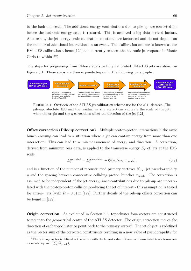
Chapter 5. Jet reconstruction 60
to the hadronic scale. The additional energy contributions due to pile-up are corrected-for
before the hadronic energy scale is restored. This is achieved using data-derived factors.
As a result, the jet energy scale calibration constants are factorised and do not depend on
the number of additional interactions in an event. This calibration scheme is known as the
EM+JES calibration scheme [120] and currently restores the hadronic jet response in Monte
Carlo to within 2%.
The steps for progressing from EM-scale jets to fully calibrated EM+JES jets are shown in
Figure 5.1. These steps are then expanded-upon in the following paragraphs.
Dag Gillberg, Carleton 2012-09-05Jet calibration schemes 6
Calorimeter jets(EM or LCW scale)
Pile-up offset correction Origin correction Energy & !
calibrationResidual in situ
calibration
Calorimeter jets(EM+JES or
LCW+JES scale)
Jet calibration
Changes the jet direction to point to the primary vertex. Does not affect the energy.
Calibrates the jet energy and pseudorapidity to the particle jet scale. Derived from MC.
Residual calibration derived using in situ measurements.Derived in data and MC. Applied only to data.
Corrects for the energy offset introduced by pile-up. Depends on µ and NPV.Derived from MC.
Jet reconstructionjet constituents jets
Local cluster weighting
Calorimeterclusters
(LCW scale)
Calorimeterclusters
(EM scale)
Jet finding Calorimeter jets(LCW scale)
Jet finding Calorimeter jets(EM scale)
Tracks Track jets
Simulatedparticles
Particle jets(aka truth jets)
Calibrates clusters based on cluster properties related to shower development
Jet finding
Jet finding
Figure 5.1: Overview of the ATLAS jet calibration scheme use for the 2011 dataset. Thepile-up, absolute JES and the residual in situ corrections calibrate the scale of the jet,while the origin and the η corrections affect the direction of the jet [121].
Offset correction (Pile-up correction) Multiple proton-proton interactions in the same
bunch crossing can lead to a situation where a jet can contain energy from more than one
interaction. This can lead to a mis-measurement of energy and direction. A correction,
derived from minimum bias data, is applied to the transverse energy ET of jets at the EM-
scale,
EcorrectedT = Euncorrected
T −O(η,NPV, τbunch), (5.2)
and is a function of the number of reconstructed primary vertexes NPV, jet pseudo-rapidity
η and the spacing between consecutive colliding proton bunches τbunch. The correction is
assumed to be independent of the jet energy, since contributions due to pile-up are uncorre-
lated with the proton-proton collision producing the jet of interest - this assumption is tested
for anti-kT jets (with R = 0.6) in [122]. Further details of the pile-up offsets correction can
be found in [122].
Origin correction As explained in Section 5.3, topocluster four-vectors are constructed
to point to the geometrical centre of the ATLAS detector. The origin correction moves the
direction of each topocluster to point back to the primary vertex6. The jet object is redefined
as the vector sum of the corrected constituents resulting in a new value of pseudorapidity for
6The primary vertex is defined as the vertex with the largest value of the sum of associated track transversemomenta squared (
∑p2T,track),
Chapter 5. Jet reconstruction 61
the jet, ηorigin. Note that the origin correction improves the angular resolution whilst leaving
the jet energy unaffected.
JES correction The final calibration step uses MC to correct jets to the hadronic scale.
Calibration constants are calculated by comparing the kinematics of MC truth jets to the
kinematics of the same jets after the full simulation of the ATLAS detector, as outlined in
Section 2.4.
Residual in-situ calibration The agreement between data and Monte Carlo is further
improved by the application of steps based on in-situ studies [122]. First, the relative response
in |η| is equalised using an inter-calibration method obtained from balancing the transverse
momenta of dijets [123]. Then, the absolute response is brought into closer agreement with
Monte Carlo by a combination of various techniques based on momentum balancing method
between photons and jets, and between high-momentum jets and a recoil system of low-
momentum jets [121]. This completes all stages of the jet calibration.
5.4.1 Jet Cleaning
Jets are classified into three categories [124]: The bad, the ugly and the good.
• Bad: Jets due to either background events or caused by detector effects
• Ugly: Jets in problematic calorimeter regions that are not well measured
• Good: Jets to be used in a physics analysis.
Three sources of bad jets are considered [124]:
• Electromagnetic coherent noise: A noise burst in occurring in the electromagnetic
(EM) liquid argon (LAr) calorimeter might lead to a “fake” jet. A large fraction of
the energy of the resulting jets comes from EM LAr calorimeter input, i.e. fLAr, or
bad-quality7 calorimeter cells., denoted by QLAr These bad jets in the EM calorimeters
are identified by requiring: fLAr > 0.95 and |QLAr| > 0.8 and QmeanLAr > 0.8 for jets with
|ηem-scale| < 2.8.
7The calorimeter quality is a measure of the difference between the measured pulse shape (ameasi ) and
the predicted pulse shape (apredi ) that is used to reconstruct the cell energy. The quality is computed as∑samples(a
measi − apredi )2.
Chapter 5. Jet reconstruction 62
• Hadronic end-cap spikes: Most “fake” jets come from sporadic noise bursts in
single calorimeter cells in the hadronic end-cap (HEC). The jets typically have a large
jet-energy fraction in the HEC, denoted by fHEC . The problematic jets in the HEC
are identified by requiring: fHEC > 0.5 and |QHEC | > 0.5 and |QLAr| > 0.8; or
|Enegative| > 60 GeV.
• Non-collision backgrounds and cosmics : Large amounts of energy can be
deposited in the calorimeter outside the nominal timing window for collisions. This is
mainly caused by cosmic ray showers or beam backgrounds. To help distinguish these
events, we identify fmax as the maximum energy fraction in one calorimeter layer, and
fcharge as the jet charge fraction: the ratio of the sum of the pT of tracks associated
to the jets divided by the calibrated jet pT . These events are identified by requiring:
fLAr < 0.05 and fcharge < 0.05 and |ηem-scale| < 2; or fEM < 0.05 and |ηem-scale| ≥ 2; or
fmax > 0.99 and |ηem-scale| < 2.
Two sources of ugly jets are considered:
• Jets extrapolated from masked cells: Permanently problematic cells and cells
affected by high voltage trips are masked during jet reconstruction and their energy
is estimated from the surrounding cells. Jets that are built from a large fraction of
these masked cells, characterised by an EM energy contribution greater than 50%, are
flagged as ugly.
• Large energy fraction in the tile-gap layers: The calibration of the scintillator
response in the gap between the hadronic tile calorimeter and the end cap is not
currently fully understood [124]. Therefore, jets with an energy fraction from this
region greater than 50% are labelled as ugly.
The effect of including these cuts on the final analysis can be seen in Table 7.2.
5.5 Jet uncertainties
Uncertainties associated with the energy scale, energy resolution and angular resolution must
be considered.
Chapter 5. Jet reconstruction 63
5.5.1 JES uncertainties
The uncertainty on the JES for a given jet is provided by the JESUncertaintyProvider (Ver-
sion 00-05-10) [121]. The jet energy scale uncertainty is determined for jets with momenta
above 15 GeV and |η| < 4.5, based on the uncertainties of the in-situ techniques and on
systematic variations in Monte Carlo simulations. For the most general case, covering all jet
measurements made in ATLAS, the correlations among JES uncertainties are described by a
set of 59 nuisance parameters. The sources of uncertainty associated with these 59 nuisance
parameters, can be assigned to one of four categories: Detector description; Physics mod-
elling; statistics and methodology; and a mix between detector and modelling effects. From
the relative η-intercalibration, the dominant uncertainty source is due to MC modelling of
jets at forward rapidities, where properties differ for the MC generators considered (Pythia
and Herwig) [121].
The fractional JES uncertainties for jets with various pT and η values is summarised in [121]:
a jet of pT = 1.5 TeV carries a fractional JES uncertainty of 3.3% across the η range. This
number can be compared to the CDF JES systematic uncertainty, which reaches values
of ∼ 3.4% for jet transverse momenta of 500 GeV [125]. The fact that ATLAS has been
above to achieve comparable JES uncertainties within two years of operation is an impressive
achievement. The DØ collaboration reported a JES uncertainty of ∼ 1.3% for central jets
with a transverse momentum of 400 GeV [126]. The impressive DØ JES uncertainty is due to
a data-driven absolute calibration - not depending upon a data-to-Monte Carlo comparison
of reconstructed physics objects. This allows avoidance of imperfect detector simulation.
An absolute calibration has not been employed by LHC experiments mainly because of the
difficulties related to the theoretical modelling at a new energy scale, however this situation
may change in the future.
Uncertainties due to pile-up, jet flavour, and jet topology are described by five additional
nuisance parameters (the uncertainty for jets originating from b quarks excluded). None of
these additional effects have an associated uncertainty in excess of 1% in the kinematic range
considered [121].
For the high pT dijet measurements made in the current analysis, the full correlation matrix
for the 59 nuisance parameters from the systematic and statistical uncertainties of in-situ
techniques is replaced by an equivalent combination of nine nuisance parameters, obtained
using a diagonalisation procedure [121]. Together with the pile-up and jet flavour uncer-
tainties, this leads to a total of 14 nuisance parameters to be propagated through the dijet
Chapter 5. Jet reconstruction 64
analysis. Details of the methodology for treatment of these 14 nuisance parameters, and the
resulting magnitudes for the effects, is given in Section 7.5.1 of this thesis.
5.5.2 Jet resolution uncertainties
The Jet Energy Resolution (JER) is defined as the width of the distribution of the relative
difference between the reconstructed energy of a given jet and its truth-level energy. The
Jet Angular Resolution (JAR) is defined as the width of the corresponding distribution
for the difference between reconstructed and truth-level η for a jet. The JER and JAR in
2011 data has been studied thoroughly but so far no result has been available outside of
the collaboration. The JER measured with the di-jet balance and the bi-sector techniques
[127, 128] in data and Monte Carlo is used to smear jets in the Monte Carlo simulation
according to the JER found in data [129]. For a given jet pT and η, if S is the corresponding
JER in MC and U is the corresponding JER uncertainty, the width of a Gaussian from where
pT and energy smearing factors are drawn randomly is:
σsmear =√
(S + U)2 − S2. (5.3)
The jet energy smearing factors, as a function of jet pT and the jet angular resolution as a
function of η are shown in Figure 5.2. After a steady reduction in the JER smearing factor
as a function of pT , the minima in Figure 5.2(a) corresponds to the range in pT where the
resolution in data and MC have the closest agreement, and therefore the JER uncertainty
is at a minimum. Figure 5.2(b) demonstrates an improvement in JAR for jets with larger
momentum, and also an improvement in JAR for larger values η.
The isolated single red cell in Figure 5.2(b) (just above 2 TeV) is caused by a single anomalous
event, with a low number of events entering that bin.
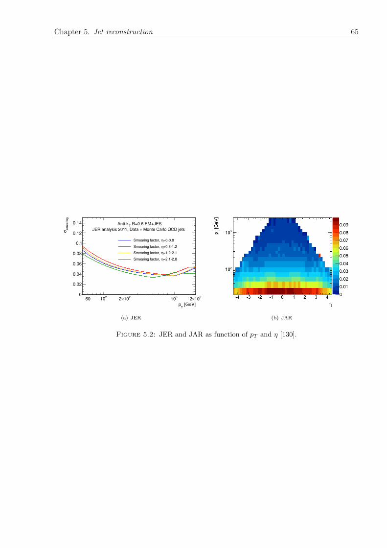
Chapter 5. Jet reconstruction 65
[GeV]T
p
60 210 210×23
103
10×2
sm
earing
σ
0
0.02
0.04
0.06
0.08
0.1
0.12
0.14
=00.8ηSmearing factor,
=0.81.2ηSmearing factor,
=1.22.1ηSmearing factor,
=2.12.8ηSmearing factor,
R=0.6 EM+JEST
Antik
JER analysis 2011, Data + Monte Carlo QCD jets
(a) JER (b) JAR
Figure 5.2: JER and JAR as function of pT and η [130].
Chapter 6
Searches for new physics with dijet
angular distributions
When two protons collide, the majority of events with large momentum transfer occur when
a parton from one hadron scatters from a parton in the other through the exchange of a
gluon or a quark. Quantum Chromodynamics (QCD) provides a good description of these
2→ 2 processes at high energies. In this chapter, the analysis of proton collisions producing
two jets, commonly known as dijet events, is discussed.
Beginning with the partonic cross-section for such dijet events in Sections 6.1, methods are
then described for disentangling the angular dependence of the partonic-cross-section from
the parton distributions functions of the colliding protons (Section 6.2). Thus, it is found
that the angular behaviour of dijet events allows the possibility to detect the presence of
New Physics (NP) signals (Section 6.4).
6.1 Leading order dijet production
6.1.1 Parton level kinematics
As a typical parton-parton hard interaction, we consider the sub-process ab → cd, where
the initial state partons a and b are contained within the colliding protons A and B - see
Figure 6.1.
66
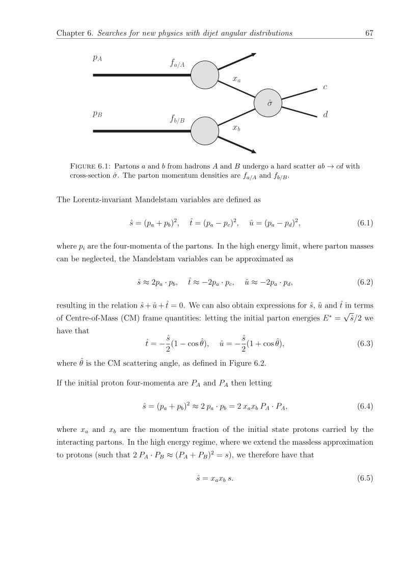
Chapter 6. Searches for new physics with dijet angular distributions 67
pA
pB
fa/A
fb/B
xa
xb
σ
c
d
Figure 6.1: Partons a and b from hadrons A and B undergo a hard scatter ab→ cd withcross-section σ. The parton momentum densities are fa/A and fb/B.
The Lorentz-invariant Mandelstam variables are defined as
s = (pa + pb)2, t = (pa − pc)2, u = (pa − pd)2, (6.1)
where pi are the four-momenta of the partons. In the high energy limit, where parton masses
can be neglected, the Mandelstam variables can be approximated as
s ≈ 2pa · pb, t ≈ −2pa · pc, u ≈ −2pa · pd, (6.2)
resulting in the relation s+ u+ t = 0. We can also obtain expressions for s, u and t in terms
of Centre-of-Mass (CM) frame quantities: letting the initial parton energies E∗ =√s/2 we
have that
t = − s2
(1− cos θ), u = − s2
(1 + cos θ), (6.3)
where θ is the CM scattering angle, as defined in Figure 6.2.
If the initial proton four-momenta are PA and PA then letting
s = (pa + pb)2 ≈ 2 pa · pb = 2 xaxb PA · PA, (6.4)
where xa and xb are the momentum fraction of the initial state protons carried by the
interacting partons. In the high energy regime, where we extend the massless approximation
to protons (such that 2 PA · PB ≈ (PA + PB)2 = s), we therefore have that
s = xaxb s. (6.5)
Chapter 6. Searches for new physics with dijet angular distributions 68
In order to relate theory and experiment, measurable quantities need to be related to kine-
matic variables in the CM frame. Since we are unable to directly measure quantities such
as s and the momenta of the initial state partons, we must relate these to the kinematics
of the final-state jets. The four-momenta of the initial state patrons can be constructed in
terms of the hadron-hadron CM energy√s to give:
pa =
√s
2(xa, 0, 0, xa) and pb =
√s
2(xb, 0, 0,−xb). (6.6)
The four-momenta of the final state partons can be constructed as:
pc = pT (cosh yc, cosφ, sinφ, sinh yc) and pd = pT (cosh yd,− cosφ,− sinφ, sinh yd) (6.7)
where yc and yd are the rapidities1 of the final state partons, which we assume to be inferable
from the rapidities of the final state jets; pT is the momentum of each of the final-state jets
in the transverse x− y plane2; and φc, φd are the azimuthal angles of the final state partons
(as introduced in Section 3.2.1). In these expressions, it is assumed that the initial-state
partons carry negligible transverse momentum and parton masses are also still neglected.
Employing energy and longitudinal momentum conservation we can combine Equations 6.6
and 6.7 to give:
xa =pT√s
(eyc + eyd) and xb =pT√s
(e−yc + e−yd). (6.8)
Using the fact that differences in rapidities are invariant under Lorentz transformations, we
define
yB(= yboost) = (yc + yd)/2 and y∗ = (yc − yd)/2, (6.9)
where ±y∗ are the rapidities of the final-state jets in the CM frame, and yB is the required
boost to move between the CM frame and the lab frame. This situation is depicted in
Figure 6.2. Combining Equations 6.8 and 6.9, and noting that cos θ∗ = tanh y∗, one is able
to show that
xa =pT√seyB cosh y∗ and xb =
pT√se−yB cosh y∗ (6.10)
and therefore
s = m2jj = xaxbs = 4p2
T cosh2 y∗, (6.11)
where mjj is the final-state dijet invariant mass.
1Rapidity is defined in Section 3.2.1.2Assuming that the initial state patrons carry zero transverse momentum, conservation of momentum
leads to the final-state jets having equal and opposite transverse momentum.
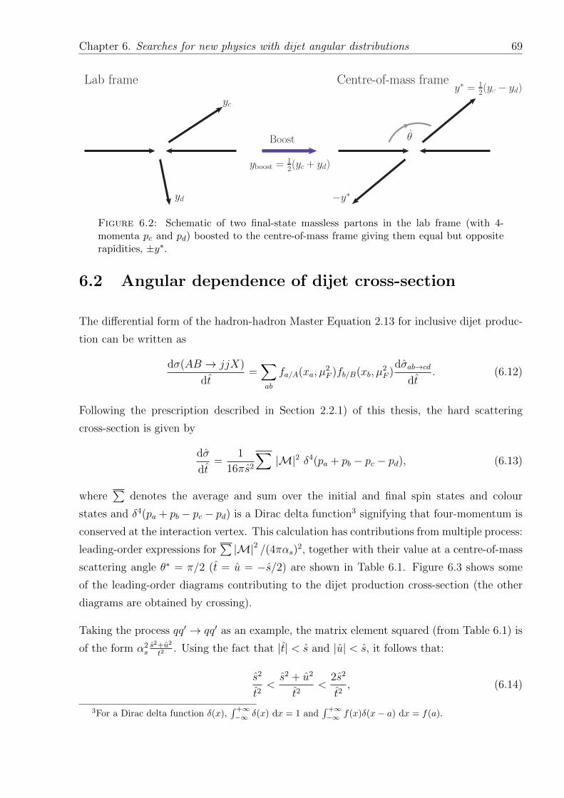
Chapter 6. Searches for new physics with dijet angular distributions 69
θ
yc
yd
y∗ = 12(yc − yd)
−y∗
yboost =12(yc + yd)
Boost
Lab frame Centre-of-mass frame
Figure 6.2: Schematic of two final-state massless partons in the lab frame (with 4-momenta pc and pd) boosted to the centre-of-mass frame giving them equal but oppositerapidities, ±y∗.
6.2 Angular dependence of dijet cross-section
The differential form of the hadron-hadron Master Equation 2.13 for inclusive dijet produc-
tion can be written as
dσ(AB → jjX)
dt=∑ab
fa/A(xa, µ2F )fb/B(xb, µ
2F )
dσab→cd
dt. (6.12)
Following the prescription described in Section 2.2.1) of this thesis, the hard scattering
cross-section is given by
dσ
dt=
1
16πs2
∑|M|2 δ4(pa + pb − pc − pd), (6.13)
where∑
denotes the average and sum over the initial and final spin states and colour
states and δ4(pa + pb − pc − pd) is a Dirac delta function3 signifying that four-momentum is
conserved at the interaction vertex. This calculation has contributions from multiple process:
leading-order expressions for∑ |M|2 /(4παs)2, together with their value at a centre-of-mass
scattering angle θ∗ = π/2 (t = u = −s/2) are shown in Table 6.1. Figure 6.3 shows some
of the leading-order diagrams contributing to the dijet production cross-section (the other
diagrams are obtained by crossing).
Taking the process qq′ → qq′ as an example, the matrix element squared (from Table 6.1) is
of the form α2ss2+u2
t2. Using the fact that |t| < s and |u| < s, it follows that:
s2
t2<s2 + u2
t2<
2s2
t2, (6.14)
3For a Dirac delta function δ(x),∫ +∞−∞ δ(x) dx = 1 and
∫ +∞−∞ f(x)δ(x− a) dx = f(a).
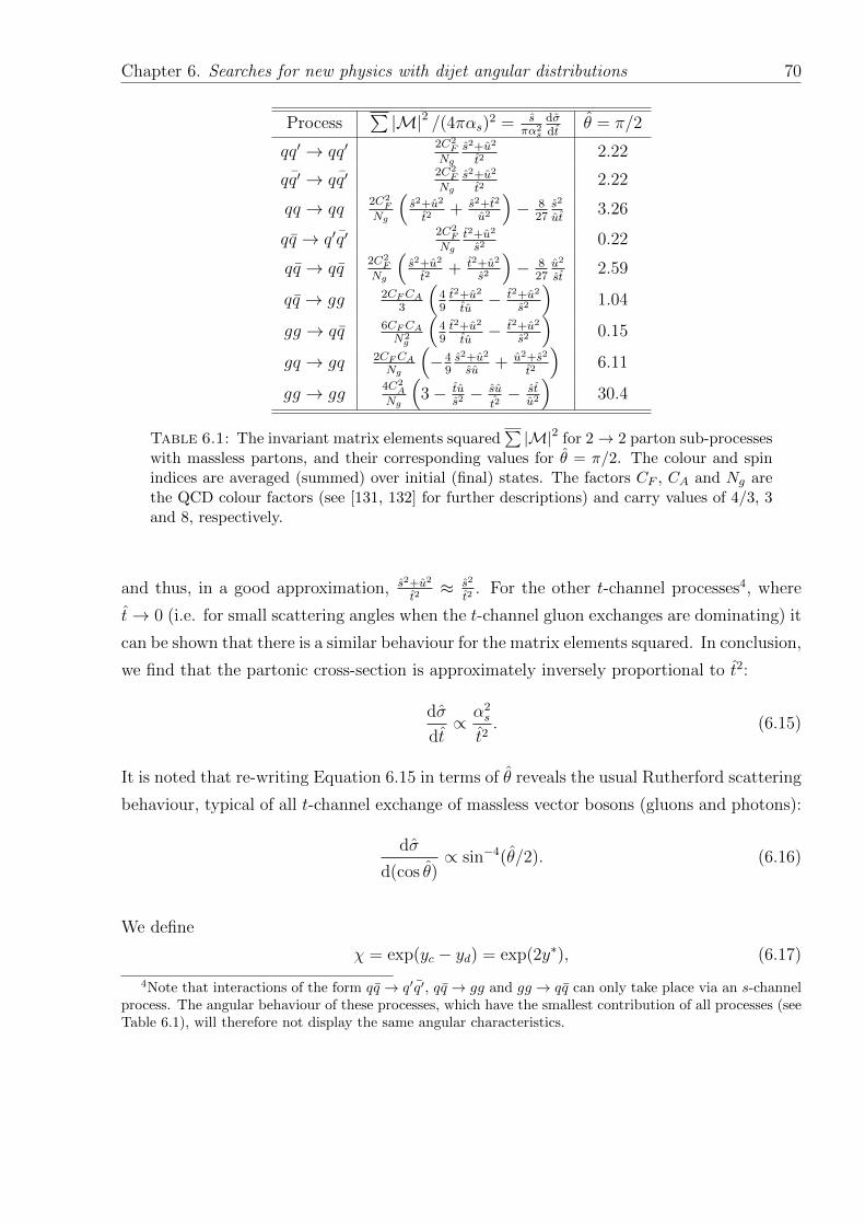
Chapter 6. Searches for new physics with dijet angular distributions 70
Process∑ |M|2 /(4παs)2 = s
πα2s
dσdt
θ = π/2
qq′ → qq′2C2
F
Ngs2+u2
t22.22
qq′ → qq′2C2
F
Ngs2+u2
t22.22
qq → qq2C2
F
Ng
(s2+u2
t2+ s2+t2
u2
)− 8
27s2
ut3.26
qq → q′q′2C2
F
Ngt2+u2
s20.22
qq → qq2C2
F
Ng
(s2+u2
t2+ t2+u2
s2
)− 8
27u2
st2.59
qq → gg 2CFCA3
(49t2+u2
tu− t2+u2
s2
)1.04
gg → qq 6CFCAN2g
(49t2+u2
tu− t2+u2
s2
)0.15
gq → gq 2CFCANg
(−4
9s2+u2
su+ u2+s2
t2
)6.11
gg → gg4C2
A
Ng
(3− tu
s2− su
t2− st
u2
)30.4
Table 6.1: The invariant matrix elements squared∑ |M|2 for 2→ 2 parton sub-processes
with massless partons, and their corresponding values for θ = π/2. The colour and spinindices are averaged (summed) over initial (final) states. The factors CF , CA and Ng arethe QCD colour factors (see [131, 132] for further descriptions) and carry values of 4/3, 3and 8, respectively.
and thus, in a good approximation, s2+u2
t2≈ s2
t2. For the other t-channel processes4, where
t→ 0 (i.e. for small scattering angles when the t-channel gluon exchanges are dominating) it
can be shown that there is a similar behaviour for the matrix elements squared. In conclusion,
we find that the partonic cross-section is approximately inversely proportional to t2:
dσ
dt∝ α2
s
t2. (6.15)
It is noted that re-writing Equation 6.15 in terms of θ reveals the usual Rutherford scattering
behaviour, typical of all t-channel exchange of massless vector bosons (gluons and photons):
dσ
d(cos θ)∝ sin−4(θ/2). (6.16)
We define
χ = exp(yc − yd) = exp(2y∗), (6.17)
4Note that interactions of the form qq → q′q′, qq → gg and gg → qq can only take place via an s-channelprocess. The angular behaviour of these processes, which have the smallest contribution of all processes (seeTable 6.1), will therefore not display the same angular characteristics.
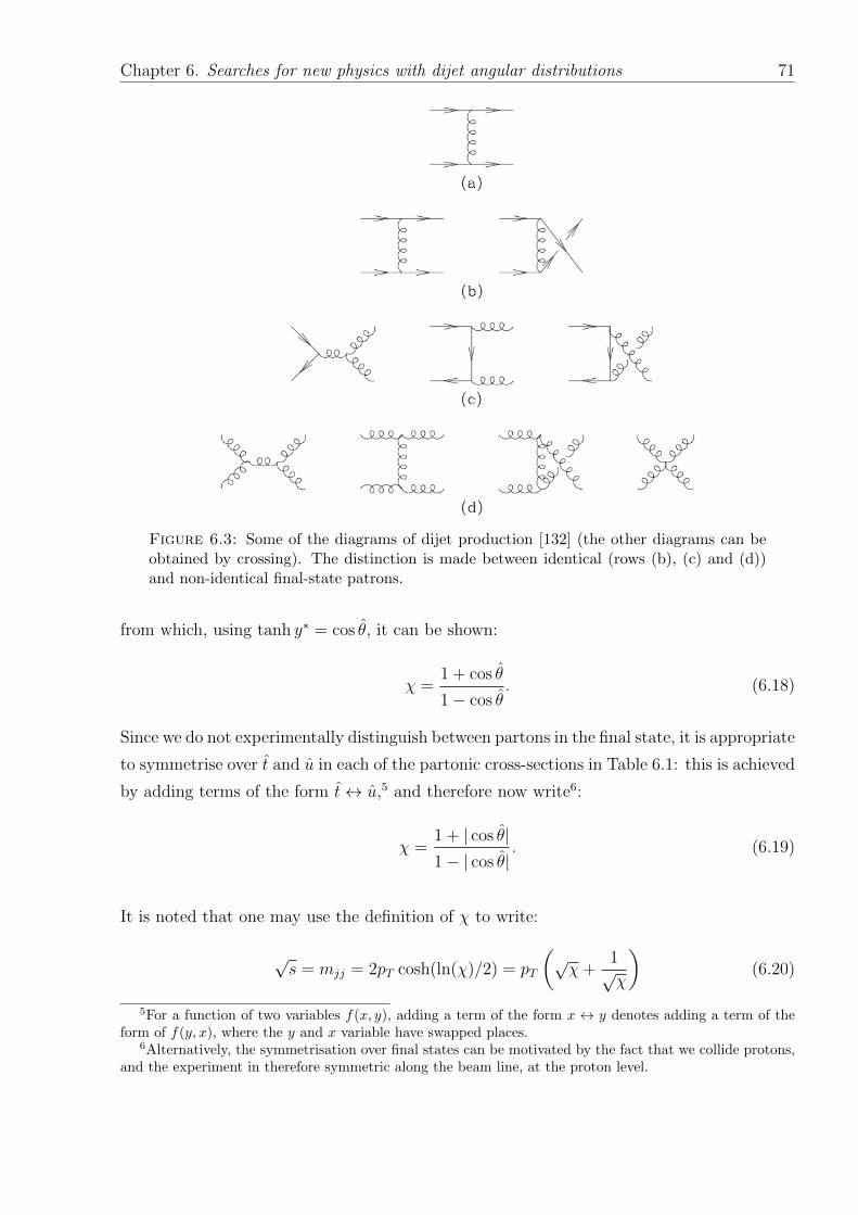
Chapter 6. Searches for new physics with dijet angular distributions 71
Figure 6.3: Some of the diagrams of dijet production [132] (the other diagrams can beobtained by crossing). The distinction is made between identical (rows (b), (c) and (d))and non-identical final-state patrons.
from which, using tanh y∗ = cos θ, it can be shown:
χ =1 + cos θ
1− cos θ. (6.18)
Since we do not experimentally distinguish between partons in the final state, it is appropriate
to symmetrise over t and u in each of the partonic cross-sections in Table 6.1: this is achieved
by adding terms of the form t↔ u,5 and therefore now write6:
χ =1 + | cos θ|1− | cos θ|
. (6.19)
It is noted that one may use the definition of χ to write:
√s = mjj = 2pT cosh(ln(χ)/2) = pT
(√χ+
1√χ
)(6.20)
5For a function of two variables f(x, y), adding a term of the form x ↔ y denotes adding a term of theform of f(y, x), where the y and x variable have swapped places.
6Alternatively, the symmetrisation over final states can be motivated by the fact that we collide protons,and the experiment in therefore symmetric along the beam line, at the proton level.
Chapter 6. Searches for new physics with dijet angular distributions 72
From this expression one can see that for a fixed√s, low values of χ correspond to high
values of pT , and vice versa.
To a good approximation,
χ =1 + | cos θ|1− | cos θ|
∼ 1
1− | cos θ|∝ s
t. (6.21)
Therefore, if one holds s fixed, we can re-write Equation 6.15 as:
dσ
dχ∝ α2
s
s(for s fixed). (6.22)
It is therefore predicted that dσ/dχ should be approximately flat, as a function of χ, for a
restricted range in s = mjj.
Alternatively, one can note that Equation 6.16 can be rewritten as
dσ
d(cos θ)∝ 1
(1− cos θ)2. (6.23)
Therefore, noticing thatdσ
dχ∝ (1− cos θ)2 dσ
d(cos θ), (6.24)
it can be seen that dσ/dχ is expected to be constant. This has been observed experimentally
in previous hadron collider experiments [133].
An isotropic angular distribution would be described by a constant value for dσ/d(cos θ).
Using Equation 6.19, we see that this would result in a a distribution of the form:
dσ
dχ∝ 1
(χ+ 1)2, (6.25)
and a cross-section in χ that is peaked at low χ values.
The difference in the χ behaviour for t-channel gluon exchange processes (such as dominant
SM QCD processes), and an s-channel process with isotropic angular distribution makes χ
an attractive variable for NP searches. This idea is further-developed in Section 6.4.
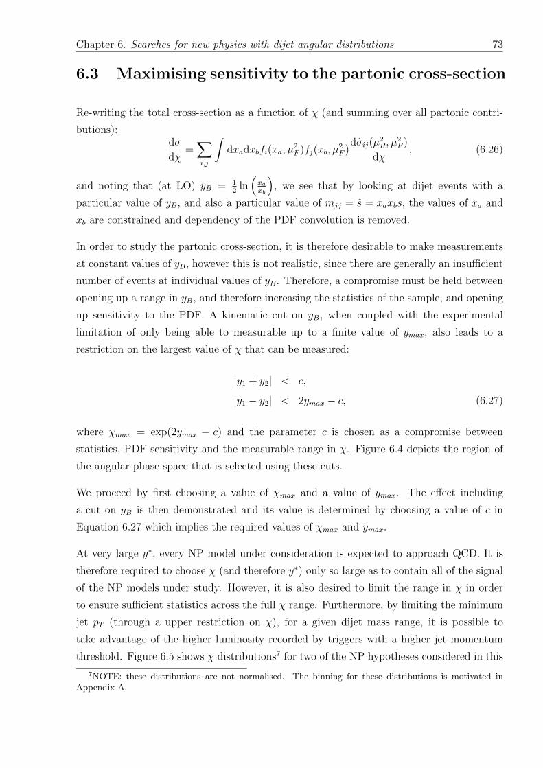
Chapter 6. Searches for new physics with dijet angular distributions 73
6.3 Maximising sensitivity to the partonic cross-section
Re-writing the total cross-section as a function of χ (and summing over all partonic contri-
butions):dσ
dχ=∑i,j
∫dxadxbfi(xa, µ
2F )fj(xb, µ
2F )
dσij(µ2R, µ
2F )
dχ, (6.26)
and noting that (at LO) yB = 12
ln(xaxb
), we see that by looking at dijet events with a
particular value of yB, and also a particular value of mjj = s = xaxbs, the values of xa and
xb are constrained and dependency of the PDF convolution is removed.
In order to study the partonic cross-section, it is therefore desirable to make measurements
at constant values of yB, however this is not realistic, since there are generally an insufficient
number of events at individual values of yB. Therefore, a compromise must be held between
opening up a range in yB, and therefore increasing the statistics of the sample, and opening
up sensitivity to the PDF. A kinematic cut on yB, when coupled with the experimental
limitation of only being able to measurable up to a finite value of ymax, also leads to a
restriction on the largest value of χ that can be measured:
|y1 + y2| < c,
|y1 − y2| < 2ymax − c, (6.27)
where χmax = exp(2ymax − c) and the parameter c is chosen as a compromise between
statistics, PDF sensitivity and the measurable range in χ. Figure 6.4 depicts the region of
the angular phase space that is selected using these cuts.
We proceed by first choosing a value of χmax and a value of ymax. The effect including
a cut on yB is then demonstrated and its value is determined by choosing a value of c in
Equation 6.27 which implies the required values of χmax and ymax.
At very large y∗, every NP model under consideration is expected to approach QCD. It is
therefore required to choose χ (and therefore y∗) only so large as to contain all of the signal
of the NP models under study. However, it is also desired to limit the range in χ in order
to ensure sufficient statistics across the full χ range. Furthermore, by limiting the minimum
jet pT (through a upper restriction on χ), for a given dijet mass range, it is possible to
take advantage of the higher luminosity recorded by triggers with a higher jet momentum
threshold. Figure 6.5 shows χ distributions7 for two of the NP hypotheses considered in this
7NOTE: these distributions are not normalised. The binning for these distributions is motivated inAppendix A.
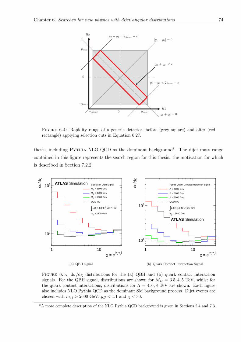
Chapter 6. Searches for new physics with dijet angular distributions 74
0
0
|y1 − y2| = 0
y2
y1y1 + y2 = 0
−ymax
ymax
−ymax ymax
y2 − y1 = 2ymax − c
y1 − y2 < 2ymax − c
|y1 + y2| < c
Figure 6.4: Rapidity range of a generic detector, before (grey square) and after (redrectangle) applying selection cuts in Equation 6.27.
thesis, including Pythia NLO QCD as the dominant background8. The dijet mass range
contained in this figure represents the search region for this thesis: the motivation for which
is described in Section 7.2.2.
|2
-y1
|y = eχ
1 10
χ/dσd
210
310 BlackMax QBH Signal
= 3500 GeVDM
= 4000 GeVDM
= 5000 GeVDM
QCD MC
=7 TeVs, -1dt = 4.8 fbL∫ > 2600 GeVjjm
ATLAS Simulation
(a) QBH signal
|2
-y1
|y = eχ
1 10
χ/dσd
210
310
Pythia Quark Contact Interaction Signal
= 4000 GeVΛ
= 6000 GeVΛ
= 8000 GeVΛ
QCD MC
=7 TeVs, -1dt = 4.8 fbL∫ > 2600 GeVjjm
ATLAS Simulation
(b) Quark Contact Interaction Signal
Figure 6.5: dσ/dχ distributions for the (a) QBH and (b) quark contact interactionsignals. For the QBH signal, distributions are shown for MD = 3.5, 4, 5 TeV, whilst forthe quark contact interactions, distributions for Λ = 4, 6, 8 TeV are shown. Each figurealso includes NLO Pythia QCD as the dominant SM background process. Dijet events arechosen with mjj > 2600 GeV, yB < 1.1 and χ < 30.
8A more complete description of the NLO Pythia QCD background is given in Sections 2.4 and 7.3.
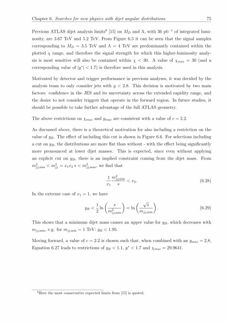
Chapter 6. Searches for new physics with dijet angular distributions 75
Previous ATLAS dijet analysis limits9 [15] on MD and Λ, with 36 pb−1 of integrated lumi-
nosity, are 3.67 TeV and 5.2 TeV. From Figure 6.5 it can be seen that the signal samples
corresponding to MD = 3.5 TeV and Λ = 4 TeV are predominantly contained within the
plotted χ range, and therefore the signal strength for which this higher-luminosity analy-
sis is most sensitive will also be contained within χ < 30. A value of χmax = 30 (and a
corresponding value of |y∗| < 1.7) is therefore used in this analysis.
Motivated by detector and trigger performance in previous analyses, it was decided by the
analysis team to only consider jets with y < 2.8. This decision is motivated by two main
factors: confidence in the JES and its uncertainty across the extended rapidity range, and
the desire to not consider triggers that operate in the forward region. In future studies, it
should be possible to take further advantage of the full ATLAS geometry.
The above restrictions on χmax and ymax are consistent with a value of c = 2.2.
As discussed above, there is a theoretical motivation for also including a restriction on the
value of yB. The effect of including this cut is shown in Figure 6.6. For selections including
a cut on yB, the distributions are more flat than without - with the effect being significantly
more pronounced at lower dijet masses. This is expected, since even without applying
an explicit cut on yB, there is an implied constraint coming from the dijet mass. From
m2jj,min < m2
jj = x1x2 s < m2jj,max, we find that
1
x1
m2jj,min
s< x2. (6.28)
In the extreme case of x1 = 1, we have
yB <1
2ln
(s
m2jj,min
)= ln
( √s
mjj,min
). (6.29)
This shows that a minimum dijet mass causes an upper value for yB, which decreases with
mjj,min, e.g. for mjj,min = 1 TeV: yB < 1.95.
Moving forward, a value of c = 2.2 is chosen such that, when combined with an ymax = 2.8,
Equation 6.27 leads to restrictions of yB < 1.1, y∗ < 1.7 and χmax = 29.9641.
9Here the most conservative expected limits from [15] is quoted.
Chapter 6. Searches for new physics with dijet angular distributions 76
|2
-y1
|y = eχ
1 10
χ/dσ
) d
σ(1
/
0.02
0.025
0.03
0.035
0.04
0.045
0.05
Pythia NLO QCD MC
|/2 < 1.12
+y1
| = |yB
|y
| < 2.82
|, |y1
|y
=7 TeVs, -1dt = 4.8 fbL∫ < 1200jj800 < m
ATLAS Simulation
(a)
|2
-y1
|y = eχ
1 10
χ/dσ
) d
σ(1
/
Pythia NLO QCD MC
|/2 < 1.12
+y1
| = |yB
|y
| < 2.82
|, |y1
|y
=7 TeVs, -1dt = 4.8 fbL∫ < 1600jj1200 < m
ATLAS Simulation
(b)
|2
-y1
|y = eχ
1 10
χ/dσ
) d
σ(1
/
0.02
0.025
0.03
0.035
0.04
0.045
0.05
Pythia NLO QCD MC
|/2 < 1.12
+y1
| = |yB
|y
| < 2.82
|, |y1
|y
=7 TeVs, -1dt = 4.8 fbL∫ < 2000jj1600 < m
ATLAS Simulation
(c)
|2
-y1
|y = eχ
1 10
χ/dσ
) d
σ(1
/
0.02
0.025
0.03
0.035
0.04
0.045
0.05
Pythia NLO QCD MC
|/2 < 1.12
+y1
| = |yB
|y
| < 2.82
|, |y1
|y
=7 TeVs, -1dt = 4.8 fbL∫ < 2600jj2000 < m
ATLAS Simulation
(d)
|2
-y1
|y = eχ
1 10
χ/dσ
) d
σ(1
/
0.02
0.025
0.03
0.035
0.04
0.045
0.05
Pythia NLO QCD MC
|/2 < 1.12
+y1
| = |yB
|y
| < 2.82
|, |y1
|y
=7 TeVs, -1dt = 4.8 fbL∫ < 7000jj2600 < m
ATLAS Simulation
(e)
Figure 6.6: Normalised χ distributions to demonstrate effect of including yB cut.
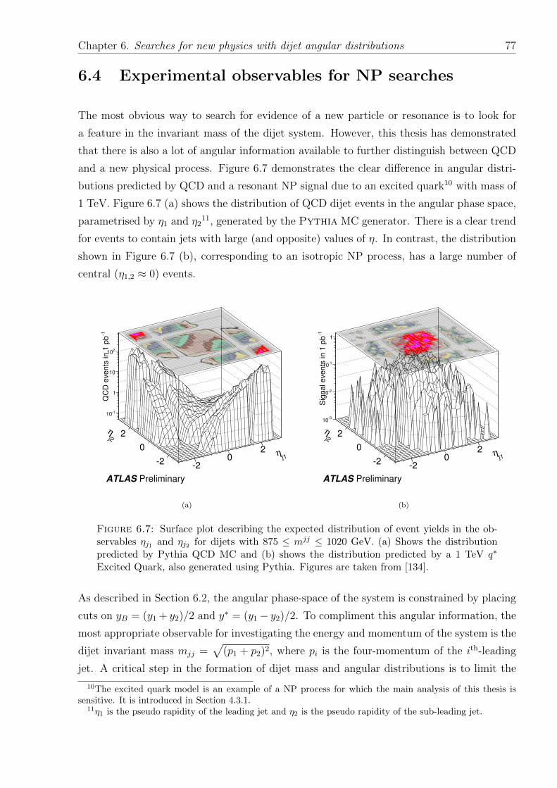
Chapter 6. Searches for new physics with dijet angular distributions 77
6.4 Experimental observables for NP searches
The most obvious way to search for evidence of a new particle or resonance is to look for
a feature in the invariant mass of the dijet system. However, this thesis has demonstrated
that there is also a lot of angular information available to further distinguish between QCD
and a new physical process. Figure 6.7 demonstrates the clear difference in angular distri-
butions predicted by QCD and a resonant NP signal due to an excited quark10 with mass of
1 TeV. Figure 6.7 (a) shows the distribution of QCD dijet events in the angular phase space,
parametrised by η1 and η211, generated by the Pythia MC generator. There is a clear trend
for events to contain jets with large (and opposite) values of η. In contrast, the distribution
shown in Figure 6.7 (b), corresponding to an isotropic NP process, has a large number of
central (η1,2 ≈ 0) events.
j1η
20
2
j2η
2
0
2
1Q
CD
eve
nts
in
1 p
b
110
1
10
210
ATLAS Preliminary
(a)
j1η
20
2
j2η
2
0
2
1S
ign
al e
ve
nts
in
1 p
b
310
210
110
1
ATLAS Preliminary
(b)
Figure 6.7: Surface plot describing the expected distribution of event yields in the ob-servables ηj1 and ηj2 for dijets with 875 ≤ mjj ≤ 1020 GeV. (a) Shows the distributionpredicted by Pythia QCD MC and (b) shows the distribution predicted by a 1 TeV q∗
Excited Quark, also generated using Pythia. Figures are taken from [134].
As described in Section 6.2, the angular phase-space of the system is constrained by placing
cuts on yB = (y1 + y2)/2 and y∗ = (y1− y2)/2. To compliment this angular information, the
most appropriate observable for investigating the energy and momentum of the system is the
dijet invariant mass mjj =√
(p1 + p2)2, where pi is the four-momentum of the ith-leading
jet. A critical step in the formation of dijet mass and angular distributions is to limit the
10The excited quark model is an example of a NP process for which the main analysis of this thesis issensitive. It is introduced in Section 4.3.1.
11η1 is the pseudo rapidity of the leading jet and η2 is the pseudo rapidity of the sub-leading jet.
Chapter 6. Searches for new physics with dijet angular distributions 78
phase space to regions where signals associated with NP are most likely to appear. The
phase space covered in the current studies is determined by rapidity selection applied to the
leading jets and their combined dijet mass.
6.4.1 Slicing the dijet phase space
For a given value of yB, the kinematic phase space of the dijet system can be parametrised
by χ and mjj. The aim of this analysis is therefore to compare the observed χ − mjj
distribution with the predicted distribution from QCD MC. In principle, one could consider
one 2-dimensional distribution finely binned in χ and in mjj, but the collision event statistics
are insufficient for this to be practical, particularly at the highest dijet masses where new
phenomena would be expect to appear. The two-dimensional phase-space is therefore sliced
in two ways:
• Large slices in mjj and small slices in χ,
• Small slices in mjj and large slices in χ.
Whilst the first method provides greater sensitivity to the angular behaviour, the second
method is more sensitive to the case of a NP signal with the form of a narrow resonance.
For the first method, distributions of dσ/dχ are plotted for large ranges of dijet mass. For
example, in a recent ATLAS dijet publication [15], mass ranges of 520 < mjj < 800 GeV,
800 < mjj < 1200 GeV, 1200 < mjj < 1600 GeV, 1600 < mjj < 2000 GeV and
mjj > 2000 GeV were used. These mass ranges, and the mass ranges used in this the-
sis, are motivated by the performance of the single jet triggers available (see Section 7.2.2
for a further description). The resulting χ distributions are normalised in order to reduce
sensitivity to systematic uncertainties12.
For the second method, a new13 variable is introduced: Fχ is the fraction of dijets produced
centrally versus the total number of observed dijets for a specified dijet mass range. This
12Normalisation of the distribution eliminates sensitivity to the luminosity uncertainty of the data, andalso reduces sensitivity to other systematic uncertainties. A full discussion is included in Section 7.4 andSection 7.5.1.
13This variable was used for the first time in [15].
Chapter 6. Searches for new physics with dijet angular distributions 79
definition is extended to a measure that is finely binned in dijet mass intervals:
Fχ([mminjj +mmax
jj ]/2) =Nevents(χ < χinner,m
minjj ,mmax
jj )
Nevents(χ < 30,mminjj ,mmax
jj )(6.30)
=Nevents(|y∗| < |y∗inner|,mmin
jj ,mmaxjj )
Nevents(|y∗| < 1.7,mminjj ,mmax
jj ), (6.31)
where Nevents is the number of candidate events with in the χ (or y∗) interval and in the
specified mjj range. From this point forward, the variable will be referred to as Fχ(mjj).
The interval χ < χinner (|y∗| < |y∗inner|) defines the central region, where we expect to be
most sensitive to new physics, while χ < 30 (|y∗| < 1.7) extends the angular range to where
QCD processes dominate. Determination of a value for χinner and y∗inner is explained in
Section 6.4.2.
As explained in Section 6.2, Equation 6.22 demonstrates that for a fixed value of s, and
therefore a fixed value of mjj, the χ distribution for QCD is expected to be flat. It is
therefore expected that the fraction of QCD events with low χ (and therefore Fχ(mjj)) will
remain constant, when finely binned in mjj. This result is demonstrated in Figure 6.9.
New phenomena that are localised near a given dijet mass would typically show up as
bumps (“resonances”) above background in the Fχ(mjj) distributions, with the latter being
due to signal events being more isotropic than the QCD background. The same excess of
central scatters could conceivably be detected above background in one χ distribution as an
excess at low χ, providing that the signal is large enough. The Fχ(mjj) distribution can
also map the mass dependence of slow-onset phenomena, such as quark contact interactions
from sensitivity to the appearance of greater centrality in the angular distributions. The χ
distributions give up some resolution in mjj in order to achieve a high precision measurement
of the changing shape of the angular distribution as mjj rises.
Normalised χ and Fχ(mjj) distributions are shown in Figures 6.8 and Figures 6.9, for the
NP signals introduced in Chapter 4. For the Fχ(mjj) distributions in Figure 6.9, a value
of χinner = 3.32 (|y∗| < 0.6) has been chosen. In the figures, a clear difference can be seen
between the QCD background and the NP signals - where the difference reduces at the value
of the each of the model parameters increases. This effect is in-line with the discussions
of Chapter 4, where we reasoned that, due to the limited partonic collision energy, the
production cross-section for each of the NP processes would reduce as the resonance mass
or threshold mass increased.
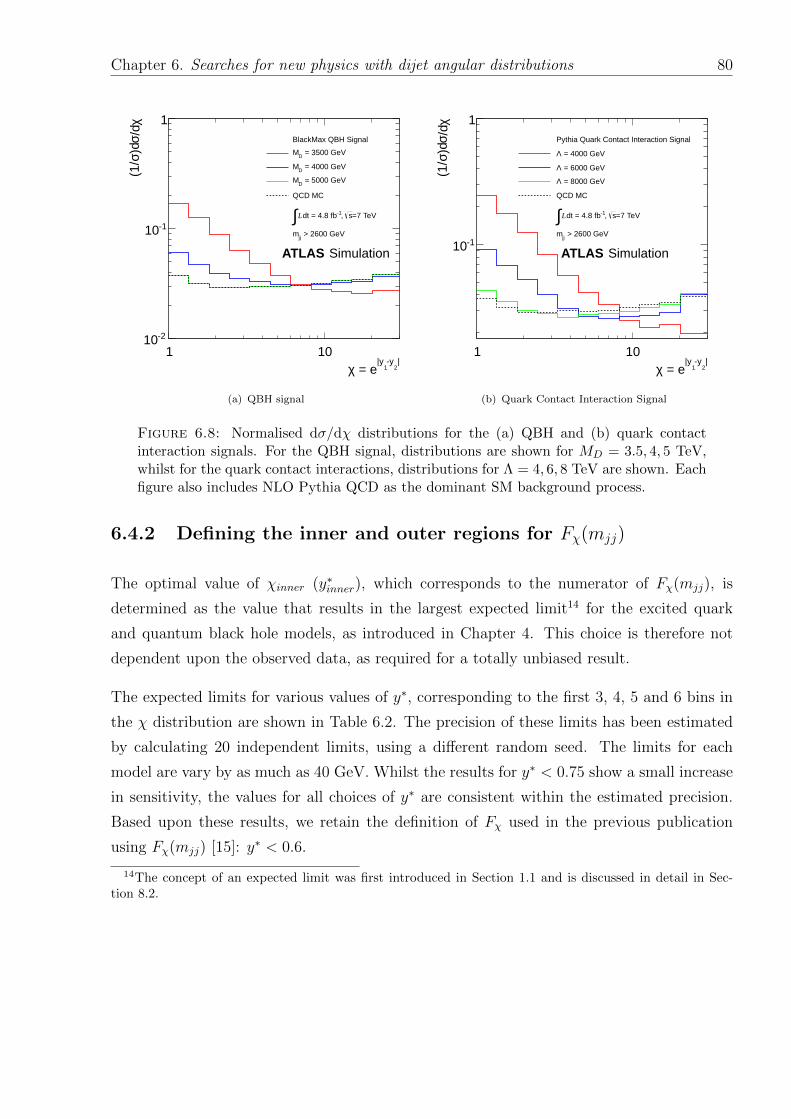
Chapter 6. Searches for new physics with dijet angular distributions 80
|2
-y1
|y = eχ
1 10
χ/dσ
)dσ(1
/
-210
-110
1BlackMax QBH Signal
= 3500 GeVDM
= 4000 GeVDM
= 5000 GeVDM
QCD MC
=7 TeVs, -1dt = 4.8 fbL∫ > 2600 GeVjjm
ATLAS Simulation
(a) QBH signal
|2
-y1
|y = eχ
1 10
χ/dσ
)dσ(1
/
-110
1Pythia Quark Contact Interaction Signal
= 4000 GeVΛ
= 6000 GeVΛ
= 8000 GeVΛ
QCD MC
=7 TeVs, -1dt = 4.8 fbL∫ > 2600 GeVjjm
ATLAS Simulation
(b) Quark Contact Interaction Signal
Figure 6.8: Normalised dσ/dχ distributions for the (a) QBH and (b) quark contactinteraction signals. For the QBH signal, distributions are shown for MD = 3.5, 4, 5 TeV,whilst for the quark contact interactions, distributions for Λ = 4, 6, 8 TeV are shown. Eachfigure also includes NLO Pythia QCD as the dominant SM background process.
6.4.2 Defining the inner and outer regions for Fχ(mjj)
The optimal value of χinner (y∗inner), which corresponds to the numerator of Fχ(mjj), is
determined as the value that results in the largest expected limit14 for the excited quark
and quantum black hole models, as introduced in Chapter 4. This choice is therefore not
dependent upon the observed data, as required for a totally unbiased result.
The expected limits for various values of y∗, corresponding to the first 3, 4, 5 and 6 bins in
the χ distribution are shown in Table 6.2. The precision of these limits has been estimated
by calculating 20 independent limits, using a different random seed. The limits for each
model are vary by as much as 40 GeV. Whilst the results for y∗ < 0.75 show a small increase
in sensitivity, the values for all choices of y∗ are consistent within the estimated precision.
Based upon these results, we retain the definition of Fχ used in the previous publication
using Fχ(mjj) [15]: y∗ < 0.6.
14The concept of an expected limit was first introduced in Section 1.1 and is discussed in detail in Sec-tion 8.2.
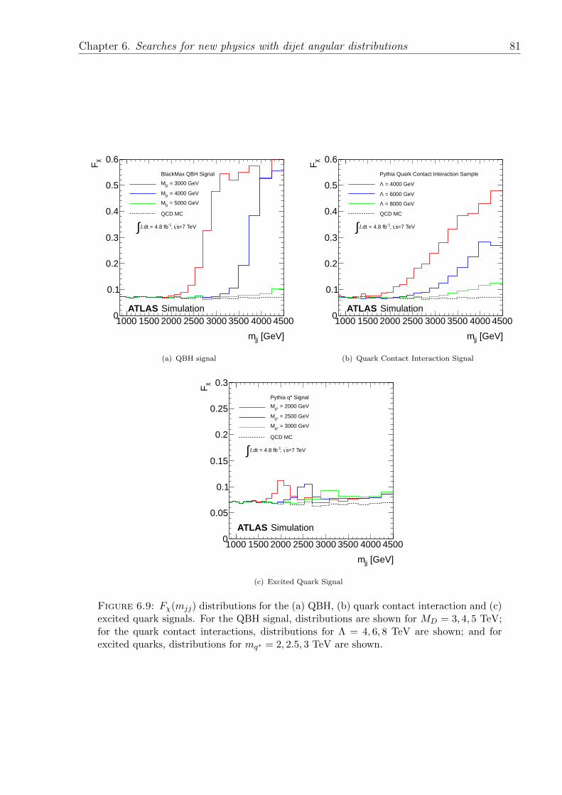
Chapter 6. Searches for new physics with dijet angular distributions 81
[GeV]jjm
1000 1500 2000 2500 3000 3500 4000 4500
χF
0
0.1
0.2
0.3
0.4
0.5
0.6
BlackMax QBH Signal
= 3000 GeVDM
= 4000 GeVDM
= 5000 GeVDM
QCD MC
=7 TeVs, -1dt = 4.8 fbL∫
ATLAS Simulation
(a) QBH signal
[GeV]jjm
1000 1500 2000 2500 3000 3500 4000 4500χ
F0
0.1
0.2
0.3
0.4
0.5
0.6
Pythia Quark Contact Interaction Sample
= 4000 GeVΛ
= 6000 GeVΛ
= 8000 GeVΛ
QCD MC
=7 TeVs, -1dt = 4.8 fbL∫
ATLAS Simulation
(b) Quark Contact Interaction Signal
[GeV]jjm
1000 1500 2000 2500 3000 3500 4000 4500
χF
0
0.05
0.1
0.15
0.2
0.25
0.3
Pythia q* Signal
= 2000 GeVq*M
= 2500 GeVq*M
= 3000 GeVq*M
QCD MC
=7 TeVs, -1dt = 4.8 fbL∫
ATLAS Simulation
(c) Excited Quark Signal
Figure 6.9: Fχ(mjj) distributions for the (a) QBH, (b) quark contact interaction and (c)excited quark signals. For the QBH signal, distributions are shown for MD = 3, 4, 5 TeV;for the quark contact interactions, distributions for Λ = 4, 6, 8 TeV are shown; and forexcited quarks, distributions for mq∗ = 2, 2.5, 3 TeV are shown.
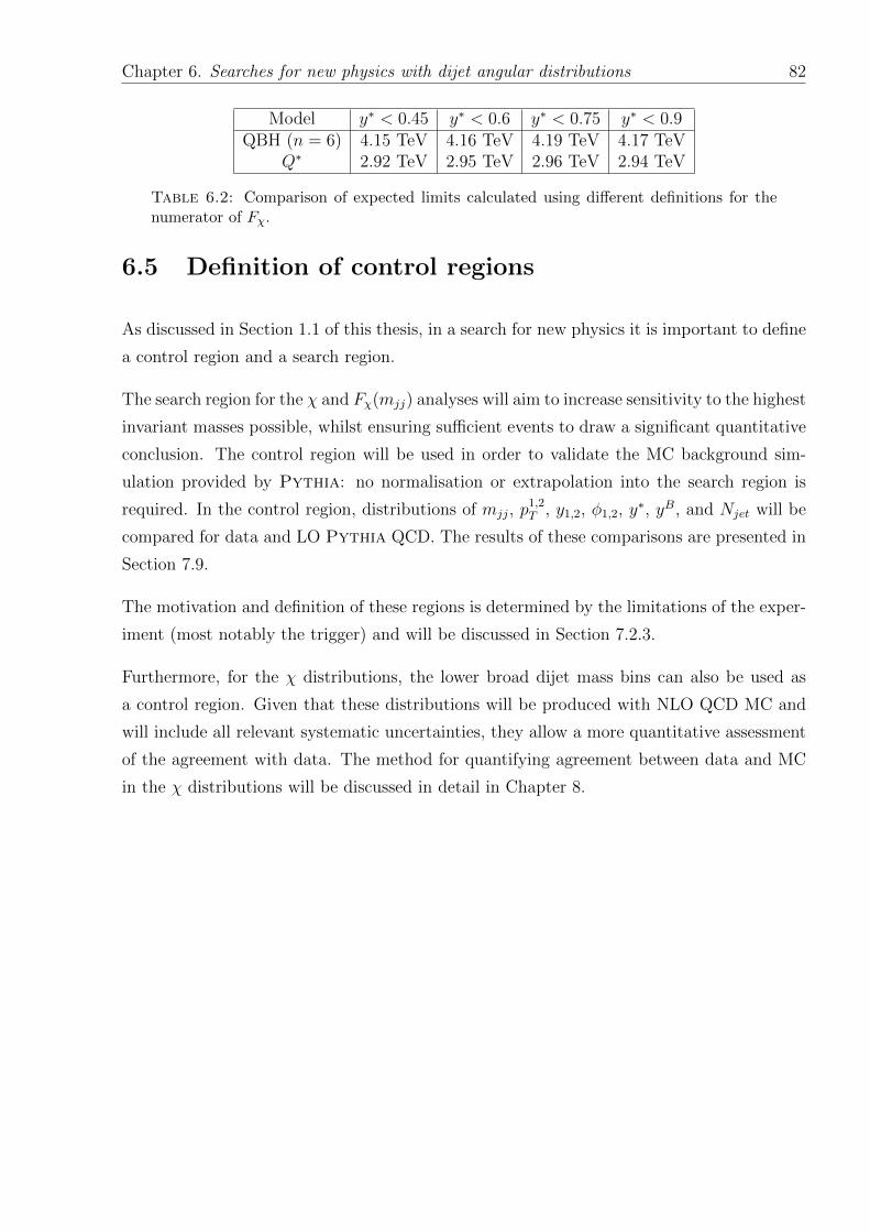
Chapter 6. Searches for new physics with dijet angular distributions 82
Model y∗ < 0.45 y∗ < 0.6 y∗ < 0.75 y∗ < 0.9QBH (n = 6) 4.15 TeV 4.16 TeV 4.19 TeV 4.17 TeV
Q∗ 2.92 TeV 2.95 TeV 2.96 TeV 2.94 TeV
Table 6.2: Comparison of expected limits calculated using different definitions for thenumerator of Fχ.
6.5 Definition of control regions
As discussed in Section 1.1 of this thesis, in a search for new physics it is important to define
a control region and a search region.
The search region for the χ and Fχ(mjj) analyses will aim to increase sensitivity to the highest
invariant masses possible, whilst ensuring sufficient events to draw a significant quantitative
conclusion. The control region will be used in order to validate the MC background sim-
ulation provided by Pythia: no normalisation or extrapolation into the search region is
required. In the control region, distributions of mjj, p1,2T , y1,2, φ1,2, y∗, yB, and Njet will be
compared for data and LO Pythia QCD. The results of these comparisons are presented in
Section 7.9.
The motivation and definition of these regions is determined by the limitations of the exper-
iment (most notably the trigger) and will be discussed in Section 7.2.3.
Furthermore, for the χ distributions, the lower broad dijet mass bins can also be used as
a control region. Given that these distributions will be produced with NLO QCD MC and
will include all relevant systematic uncertainties, they allow a more quantitative assessment
of the agreement with data. The method for quantifying agreement between data and MC
in the χ distributions will be discussed in detail in Chapter 8.
Chapter 7
Event selection, systematic
uncertainties and resulting
distributions
Building upon the theoretical and experimental foundations of previous chapters, this chapter
will discuss the analysis strategy and its results, with full consideration for the associated
experimental and theoretical uncertainties. The motivation for event selection criteria is
formed from a combination of sensitivity to New Physics, fiducial experimental constraints
and limitations of detector performance.
Details of the systematic uncertainties arising from Jet Energy Scale and Resolution are de-
scribed in Section 7.5.1. The corresponding theoretical systematic uncertainties for the QCD
background description are described in Section 7.4. Additional possible uncertainty consid-
erations due to the experimental conditions of Pile-up (Section 7.7) and detector malfunction
(Section 7.8) are given at the end of the chapter.
Final distributions for this analysis are shown in Figure 7.10 and their statistical interpre-
tation is described in Chapter 8.
7.1 Event selection
In this section, the motivation and details for the analysis event selection is given. Each of
the selection criteria is outlined below, with a summary of the resulting number of events
after each cut summarised in Table 7.2. The initial number of events under consideration
83
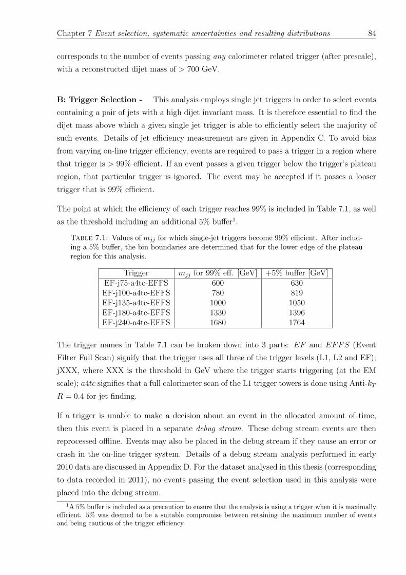
Chapter 7 Event selection, systematic uncertainties and resulting distributions 84
corresponds to the number of events passing any calorimeter related trigger (after prescale),
with a reconstructed dijet mass of > 700 GeV.
B: Trigger Selection - This analysis employs single jet triggers in order to select events
containing a pair of jets with a high dijet invariant mass. It is therefore essential to find the
dijet mass above which a given single jet trigger is able to efficiently select the majority of
such events. Details of jet efficiency measurement are given in Appendix C. To avoid bias
from varying on-line trigger efficiency, events are required to pass a trigger in a region where
that trigger is > 99% efficient. If an event passes a given trigger below the trigger’s plateau
region, that particular trigger is ignored. The event may be accepted if it passes a looser
trigger that is 99% efficient.
The point at which the efficiency of each trigger reaches 99% is included in Table 7.1, as well
as the threshold including an additional 5% buffer1.
Table 7.1: Values of mjj for which single-jet triggers become 99% efficient. After includ-ing a 5% buffer, the bin boundaries are determined that for the lower edge of the plateauregion for this analysis.
Trigger mjj for 99% eff. [GeV] +5% buffer [GeV]EF-j75-a4tc-EFFS 600 630EF-j100-a4tc-EFFS 780 819EF-j135-a4tc-EFFS 1000 1050EF-j180-a4tc-EFFS 1330 1396EF-j240-a4tc-EFFS 1680 1764
The trigger names in Table 7.1 can be broken down into 3 parts: EF and EFFS (Event
Filter Full Scan) signify that the trigger uses all three of the trigger levels (L1, L2 and EF);
jXXX, where XXX is the threshold in GeV where the trigger starts triggering (at the EM
scale); a4tc signifies that a full calorimeter scan of the L1 trigger towers is done using Anti-kT
R = 0.4 for jet finding.
If a trigger is unable to make a decision about an event in the allocated amount of time,
then this event is placed in a separate debug stream. These debug stream events are then
reprocessed offline. Events may also be placed in the debug stream if they cause an error or
crash in the on-line trigger system. Details of a debug stream analysis performed in early
2010 data are discussed in Appendix D. For the dataset analysed in this thesis (corresponding
to data recorded in 2011), no events passing the event selection used in this analysis were
placed into the debug stream.
1A 5% buffer is included as a precaution to ensure that the analysis is using a trigger when it is maximallyefficient. 5% was deemed to be a suitable compromise between retaining the maximum number of eventsand being cautious of the trigger efficiency.
Chapter 7 Event selection, systematic uncertainties and resulting distributions 85
C: GoodRunsList selection - Events are only considered if they fall into a luminos-
ity block contained within a centrally produced GoodRunsList. Luminosity blocks and
GoodRunsLists are both discussed in Section 10.2. Briefly, a luminosity block is a period in
time, usually lasting a few minutes, for which the instantaneous luminosity is approximately
constant, and a GoodRunsList [135] is a list of luminosity blocks, which have been deemed
suitable for a physics analysis. Criteria include stable proton beams from the LHC, detector
component temperatures, magnetic field strengths and detector status.
D: Vertex selection - Events are required to have a primary collision vertex defined by
two or more charged particle tracks. In the presence of pile-up, the primary collision vertex
is the one with the largest scalar sum of p2T for associated tracks, which insures that the
highest pT jets, used to reconstruct the dijet, have been associated with the correct collision
vertex.
E: LAr error cut - Events are rejected if the data from the liquid argon calorimeter
have an unusual topology2 or there is evidence of data corruption [136].
F: Check for number of jets - There must be at least two jets within |y| < 4.4 in
the event, and all jets with |y| ≥ 4.4 are discarded. The highest pT jet is referred to as the
“leading” jet (j1), and the second highest, as the “next-to-leading” jet (j2). The two jets are
collectively referred to as the ‘leading jets ’.
G: Ugly jet cleaning - According to the criteria described in Section 5.4.1, for events
to be retained, there must be no poorly measured jets with pT greater than 30% of the pT
of the next-to-leading jet. Poorly measured jets correspond to energy depositions in regions
where the energy measurement is known to be inaccurate.
H: LAr hole cut - A selection has been implemented to avoid an electromagnetic calorime-
ter defect in the region from -0.1 to 1.5 in η, and from -0.9 to -0.5 in φ that occurred during
part of the running period. The average energy loss for jets in this region is 20% to 30%.
Jets within ∆R = 0.1 of this region have been rejected if such jets have a pT greater than
30% of the next-to-leading jet pT. In order to retain the shape of dijet angular distributions
2Examples of an unusual jet topology include: a jet formed by a single cell in the hadronic end cap (mostlikely a noisy cell), or an out-of-time energy deposition (most likely due to a cosmic ray).
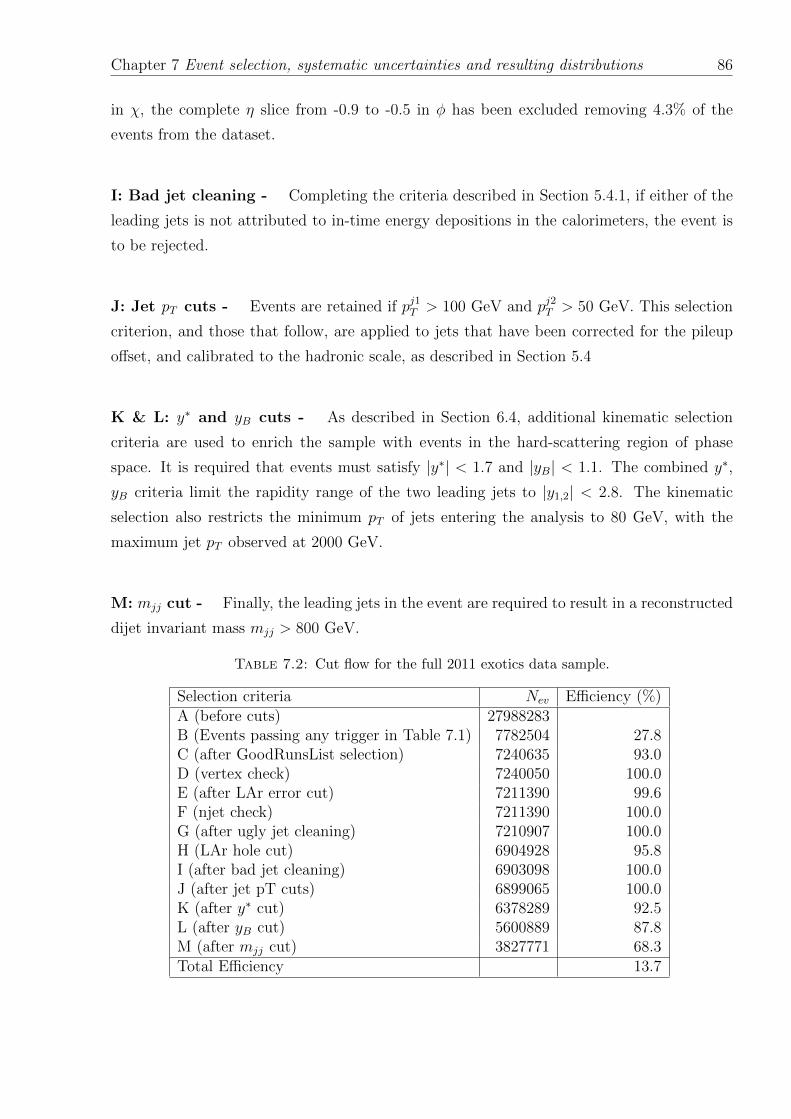
Chapter 7 Event selection, systematic uncertainties and resulting distributions 86
in χ, the complete η slice from -0.9 to -0.5 in φ has been excluded removing 4.3% of the
events from the dataset.
I: Bad jet cleaning - Completing the criteria described in Section 5.4.1, if either of the
leading jets is not attributed to in-time energy depositions in the calorimeters, the event is
to be rejected.
J: Jet pT cuts - Events are retained if pj1T > 100 GeV and pj2T > 50 GeV. This selection
criterion, and those that follow, are applied to jets that have been corrected for the pileup
offset, and calibrated to the hadronic scale, as described in Section 5.4
K & L: y∗ and yB cuts - As described in Section 6.4, additional kinematic selection
criteria are used to enrich the sample with events in the hard-scattering region of phase
space. It is required that events must satisfy |y∗| < 1.7 and |yB| < 1.1. The combined y∗,
yB criteria limit the rapidity range of the two leading jets to |y1,2| < 2.8. The kinematic
selection also restricts the minimum pT of jets entering the analysis to 80 GeV, with the
maximum jet pT observed at 2000 GeV.
M: mjj cut - Finally, the leading jets in the event are required to result in a reconstructed
dijet invariant mass mjj > 800 GeV.
Table 7.2: Cut flow for the full 2011 exotics data sample.
Selection criteria Nev Efficiency (%)A (before cuts) 27988283B (Events passing any trigger in Table 7.1) 7782504 27.8C (after GoodRunsList selection) 7240635 93.0D (vertex check) 7240050 100.0E (after LAr error cut) 7211390 99.6F (njet check) 7211390 100.0G (after ugly jet cleaning) 7210907 100.0H (LAr hole cut) 6904928 95.8I (after bad jet cleaning) 6903098 100.0J (after jet pT cuts) 6899065 100.0K (after y∗ cut) 6378289 92.5L (after yB cut) 5600889 87.8M (after mjj cut) 3827771 68.3Total Efficiency 13.7
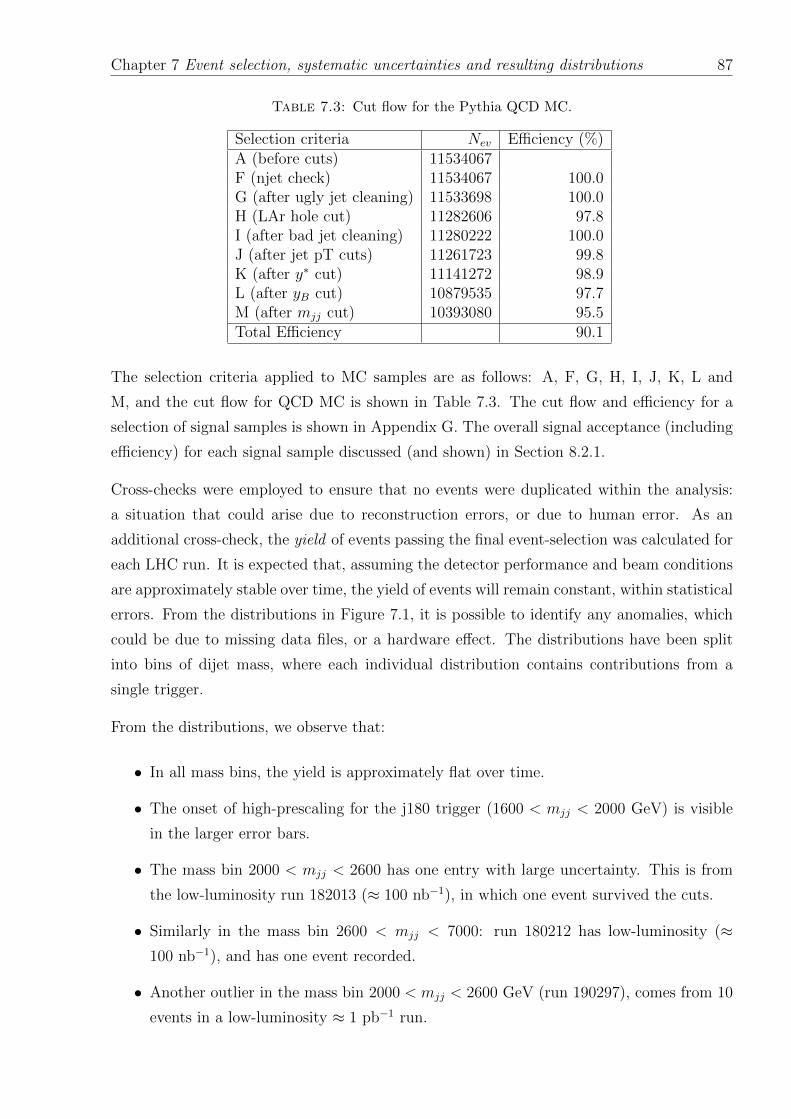
Chapter 7 Event selection, systematic uncertainties and resulting distributions 87
Table 7.3: Cut flow for the Pythia QCD MC.
Selection criteria Nev Efficiency (%)A (before cuts) 11534067F (njet check) 11534067 100.0G (after ugly jet cleaning) 11533698 100.0H (LAr hole cut) 11282606 97.8I (after bad jet cleaning) 11280222 100.0J (after jet pT cuts) 11261723 99.8K (after y∗ cut) 11141272 98.9L (after yB cut) 10879535 97.7M (after mjj cut) 10393080 95.5Total Efficiency 90.1
The selection criteria applied to MC samples are as follows: A, F, G, H, I, J, K, L and
M, and the cut flow for QCD MC is shown in Table 7.3. The cut flow and efficiency for a
selection of signal samples is shown in Appendix G. The overall signal acceptance (including
efficiency) for each signal sample discussed (and shown) in Section 8.2.1.
Cross-checks were employed to ensure that no events were duplicated within the analysis:
a situation that could arise due to reconstruction errors, or due to human error. As an
additional cross-check, the yield of events passing the final event-selection was calculated for
each LHC run. It is expected that, assuming the detector performance and beam conditions
are approximately stable over time, the yield of events will remain constant, within statistical
errors. From the distributions in Figure 7.1, it is possible to identify any anomalies, which
could be due to missing data files, or a hardware effect. The distributions have been split
into bins of dijet mass, where each individual distribution contains contributions from a
single trigger.
From the distributions, we observe that:
• In all mass bins, the yield is approximately flat over time.
• The onset of high-prescaling for the j180 trigger (1600 < mjj < 2000 GeV) is visible
in the larger error bars.
• The mass bin 2000 < mjj < 2600 has one entry with large uncertainty. This is from
the low-luminosity run 182013 (≈ 100 nb−1), in which one event survived the cuts.
• Similarly in the mass bin 2600 < mjj < 7000: run 180212 has low-luminosity (≈100 nb−1), and has one event recorded.
• Another outlier in the mass bin 2000 < mjj < 2600 GeV (run 190297), comes from 10
events in a low-luminosity ≈ 1 pb−1 run.
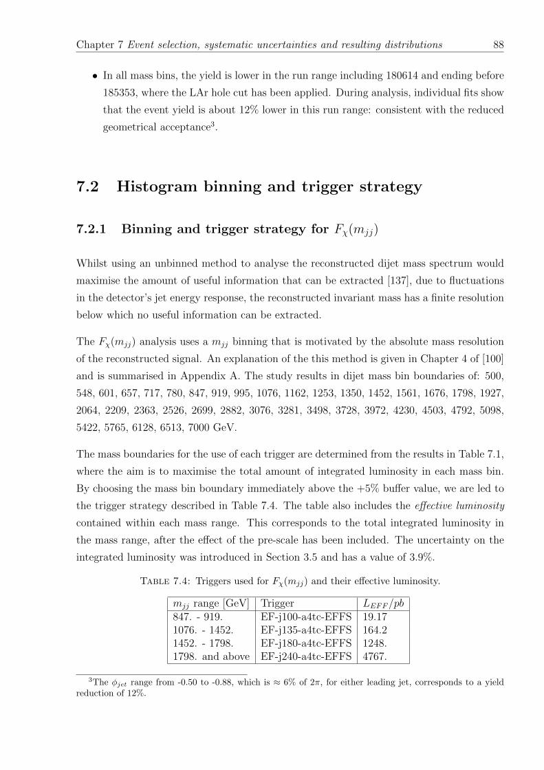
Chapter 7 Event selection, systematic uncertainties and resulting distributions 88
• In all mass bins, the yield is lower in the run range including 180614 and ending before
185353, where the LAr hole cut has been applied. During analysis, individual fits show
that the event yield is about 12% lower in this run range: consistent with the reduced
geometrical acceptance3.
7.2 Histogram binning and trigger strategy
7.2.1 Binning and trigger strategy for Fχ(mjj)
Whilst using an unbinned method to analyse the reconstructed dijet mass spectrum would
maximise the amount of useful information that can be extracted [137], due to fluctuations
in the detector’s jet energy response, the reconstructed invariant mass has a finite resolution
below which no useful information can be extracted.
The Fχ(mjj) analysis uses a mjj binning that is motivated by the absolute mass resolution
of the reconstructed signal. An explanation of the this method is given in Chapter 4 of [100]
and is summarised in Appendix A. The study results in dijet mass bin boundaries of: 500,
548, 601, 657, 717, 780, 847, 919, 995, 1076, 1162, 1253, 1350, 1452, 1561, 1676, 1798, 1927,
2064, 2209, 2363, 2526, 2699, 2882, 3076, 3281, 3498, 3728, 3972, 4230, 4503, 4792, 5098,
5422, 5765, 6128, 6513, 7000 GeV.
The mass boundaries for the use of each trigger are determined from the results in Table 7.1,
where the aim is to maximise the total amount of integrated luminosity in each mass bin.
By choosing the mass bin boundary immediately above the +5% buffer value, we are led to
the trigger strategy described in Table 7.4. The table also includes the effective luminosity
contained within each mass range. This corresponds to the total integrated luminosity in
the mass range, after the effect of the pre-scale has been included. The uncertainty on the
integrated luminosity was introduced in Section 3.5 and has a value of 3.9%.
Table 7.4: Triggers used for Fχ(mjj) and their effective luminosity.
mjj range [GeV] Trigger LEFF/pb847. - 919. EF-j100-a4tc-EFFS 19.171076. - 1452. EF-j135-a4tc-EFFS 164.21452. - 1798. EF-j180-a4tc-EFFS 1248.1798. and above EF-j240-a4tc-EFFS 4767.
3The φjet range from -0.50 to -0.88, which is ≈ 6% of 2π, for either leading jet, corresponds to a yieldreduction of 12%.
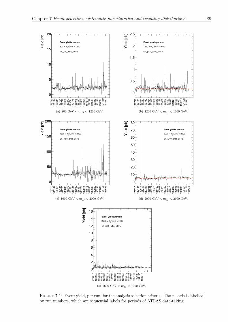
Chapter 7 Event selection, systematic uncertainties and resulting distributions 89
179710
180144
180614
182424
182726
183038
183272
183581
184169
185976
186217
186669
186934
187811
189242
189561
189813
190120
190661
191150
191517
Yie
ld [nb]
0
5
10
15
20
Event yields per run
/GeV < 1200jj
800 < m
EF_j75_a4tc_EFFS
(a) 800 GeV < mjj < 1200 GeV.
179710
180144
180614
182424
182747
183054
183347
183963
185649
186178
186456
186873
187453
189027
189421
189660
189963
190611
191138
191513
Yie
ld [nb]
0
0.5
1
1.5
2
2.5
Event yields per run
/GeV < 1600jj
1200 < m
EF_j100_a4tc_EFFS
(b) 1200 GeV < mjj < 1600 GeV.
179710
180144
180481
182424
182726
183038
183272
183581
184169
186049
186361
186729
187014
187815
189280
189598
189822
190236
190689
191190
191635
Yie
ld [pb]
0
50
100
150
200
Event yields per run
/GeV < 2000jj
1600 < m
EF_j180_a4tc_EFFS
(c) 1600 GeV < mjj < 2000 GeV.
179710
180144
180614
182424
182726
183038
183272
183581
184169
186049
186361
186729
187014
187815
189280
189598
189822
190236
190661
191150
191517
Yie
ld [pb]
0
10
20
30
40
50
60
70
80
Event yields per run
/GeV < 2600jj
2000 < m
EF_j240_a4tc_EFFS
(d) 2000 GeV < mjj < 2600 GeV.
179710
180153
180636
182516
183003
183216
183780
185731
186180
186516
186923
187552
189079
189483
189751
190116
190661
191190
191715
Yie
ld [pb]
0
2
4
6
8
10
12
14
16
Event yields per run
/GeV < 7000jj
2600 < m
EF_j240_a4tc_EFFS
(e) 2600 GeV < mjj < 7000 GeV.
Figure 7.1: Event yield, per run, for the analysis selection criteria. The x−axis is labelledby run numbers, which are sequential labels for periods of ATLAS data-taking.
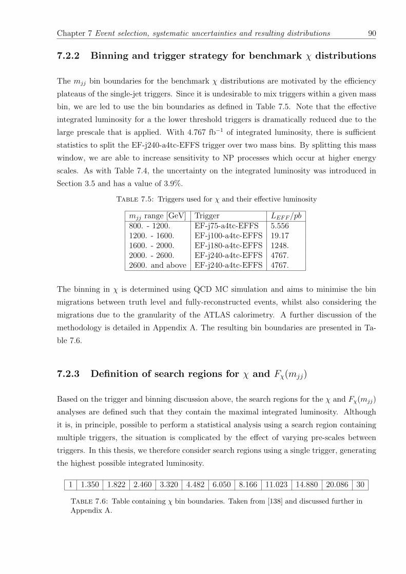
Chapter 7 Event selection, systematic uncertainties and resulting distributions 90
7.2.2 Binning and trigger strategy for benchmark χ distributions
The mjj bin boundaries for the benchmark χ distributions are motivated by the efficiency
plateaus of the single-jet triggers. Since it is undesirable to mix triggers within a given mass
bin, we are led to use the bin boundaries as defined in Table 7.5. Note that the effective
integrated luminosity for a the lower threshold triggers is dramatically reduced due to the
large prescale that is applied. With 4.767 fb−1 of integrated luminosity, there is sufficient
statistics to split the EF-j240-a4tc-EFFS trigger over two mass bins. By splitting this mass
window, we are able to increase sensitivity to NP processes which occur at higher energy
scales. As with Table 7.4, the uncertainty on the integrated luminosity was introduced in
Section 3.5 and has a value of 3.9%.
Table 7.5: Triggers used for χ and their effective luminosity
mjj range [GeV] Trigger LEFF/pb800. - 1200. EF-j75-a4tc-EFFS 5.5561200. - 1600. EF-j100-a4tc-EFFS 19.171600. - 2000. EF-j180-a4tc-EFFS 1248.2000. - 2600. EF-j240-a4tc-EFFS 4767.2600. and above EF-j240-a4tc-EFFS 4767.
The binning in χ is determined using QCD MC simulation and aims to minimise the bin
migrations between truth level and fully-reconstructed events, whilst also considering the
migrations due to the granularity of the ATLAS calorimetry. A further discussion of the
methodology is detailed in Appendix A. The resulting bin boundaries are presented in Ta-
ble 7.6.
7.2.3 Definition of search regions for χ and Fχ(mjj)
Based on the trigger and binning discussion above, the search regions for the χ and Fχ(mjj)
analyses are defined such that they contain the maximal integrated luminosity. Although
it is, in principle, possible to perform a statistical analysis using a search region containing
multiple triggers, the situation is complicated by the effect of varying pre-scales between
triggers. In this thesis, we therefore consider search regions using a single trigger, generating
the highest possible integrated luminosity.
1 1.350 1.822 2.460 3.320 4.482 6.050 8.166 11.023 14.880 20.086 30
Table 7.6: Table containing χ bin boundaries. Taken from [138] and discussed further inAppendix A.
Chapter 7 Event selection, systematic uncertainties and resulting distributions 91
Using Tables 7.4 and 7.5, the search regions for χ and Fχ(mjj) are defined as mjj > 2600 GeV
and mjj > 1798 GeV, respectively. The lower regions of these search boundaries are also
well below the current best limits on NP models, calculated with these analyses [15]: thus
reducing the possibility of missing a NP effect at lower dijet masses.
7.3 QCD predictions
In the analyses described in this thesis, the QCD prediction is based on MC generation of
Pythia 2→ 2 event samples which cover the kinematic range in χ and mjj spanned by the
selected dijet events (See Section 2.5).
In-time pileup is simulated by generating samples of minimum bias events using Pythia 6,
which are also passed through detector simulation. To simulate QCD events in the presence
of pileup, hard scattering events are overlaid with a number, µ, of minimum bias events,
where µ is Poisson distributed and 〈µ〉 is chosen to match its expected value in data. The
superposition of MC events is performed by summing simulated signals of hard scattering
and minimum bias events in each detector electronic channel.
The combined MC events, containing one hard interaction and several soft interactions,
are then reconstructed in the same way as collision data, including the jet correction and
calibration steps described in Section 5.4.
Since the MC samples have been generated based on an estimate of the average luminosity
during the 2011 data-taking, pileup reweighting is employed to adjust each MC event such
that the µ distribution for the MC sample matches the µ distribution observed in data. A
study of the effects of pile-up reweighting is included in Appendix F.
The corrected MC samples are subjected to the same event selection criteria as applied to
collision data.
7.3.1 NLO QCD calculations
Within Section 2.4, the issues surrounding simulation of QCD Monte Carlo were explained.
The main steps of simulation of the hard scattering process, the initial and final state ra-
diation, multiple interactions and the non-perturbative hadronisation results in a Leading
Order (LO) description. Whilst a LO description may provide a good description of the
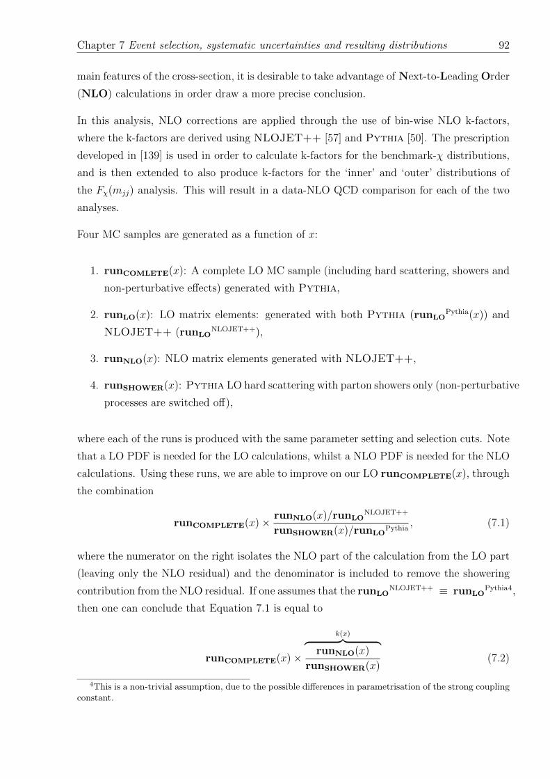
Chapter 7 Event selection, systematic uncertainties and resulting distributions 92
main features of the cross-section, it is desirable to take advantage of Next-to-Leading Order
(NLO) calculations in order draw a more precise conclusion.
In this analysis, NLO corrections are applied through the use of bin-wise NLO k-factors,
where the k-factors are derived using NLOJET++ [57] and Pythia [50]. The prescription
developed in [139] is used in order to calculate k-factors for the benchmark-χ distributions,
and is then extended to also produce k-factors for the ‘inner’ and ‘outer’ distributions of
the Fχ(mjj) analysis. This will result in a data-NLO QCD comparison for each of the two
analyses.
Four MC samples are generated as a function of x:
1. runCOMLETE(x): A complete LO MC sample (including hard scattering, showers and
non-perturbative effects) generated with Pythia,
2. runLO(x): LO matrix elements: generated with both Pythia (runLOPythia(x)) and
NLOJET++ (runLONLOJET++),
3. runNLO(x): NLO matrix elements generated with NLOJET++,
4. runSHOWER(x): Pythia LO hard scattering with parton showers only (non-perturbative
processes are switched off),
where each of the runs is produced with the same parameter setting and selection cuts. Note
that a LO PDF is needed for the LO calculations, whilst a NLO PDF is needed for the NLO
calculations. Using these runs, we are able to improve on our LO runCOMPLETE(x), through
the combination
runCOMPLETE(x)× runNLO(x)/runLONLOJET++
runSHOWER(x)/runLOPythia
, (7.1)
where the numerator on the right isolates the NLO part of the calculation from the LO part
(leaving only the NLO residual) and the denominator is included to remove the showering
contribution from the NLO residual. If one assumes that the runLONLOJET++ ≡ runLO
Pythia4,
then one can conclude that Equation 7.1 is equal to
runCOMPLETE(x)×
k(x)︷ ︸︸ ︷runNLO(x)
runSHOWER(x)(7.2)
4This is a non-trivial assumption, due to the possible differences in parametrisation of the strong couplingconstant.
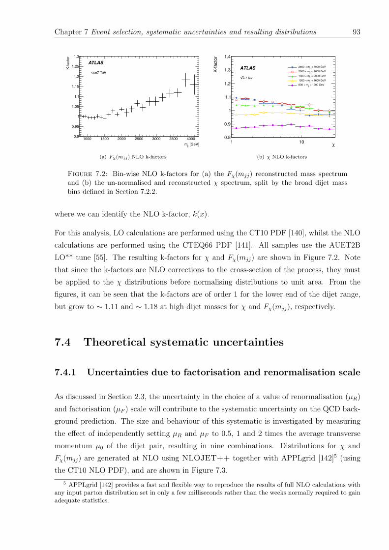
Chapter 7 Event selection, systematic uncertainties and resulting distributions 93
[GeV]jjm1000 1500 2000 2500 3000 3500 4000
K-fa
ctor
0.9
0.95
1
1.05
1.1
1.15
1.2
1.25
1.3
=7 TeVs
ATLAS
(a) Fχ(mjj) NLO k-factors
!1 10
K-fa
ctor
0.8
0.9
1
1.1
1.2
1.3
1.4
< 7000 GeVjj2600 < m
< 2600 GeVjj2000 < m
< 2000 GeVjj1600 < m
< 1600 GeVjj1200 < m
< 1200 GeVjj800 < m
ATLAS
=7 TeVs
(b) χ NLO k-factors
Figure 7.2: Bin-wise NLO k-factors for (a) the Fχ(mjj) reconstructed mass spectrumand (b) the un-normalised and reconstructed χ spectrum, split by the broad dijet massbins defined in Section 7.2.2.
where we can identify the NLO k-factor, k(x).
For this analysis, LO calculations are performed using the CT10 PDF [140], whilst the NLO
calculations are performed using the CTEQ66 PDF [141]. All samples use the AUET2B
LO** tune [55]. The resulting k-factors for χ and Fχ(mjj) are shown in Figure 7.2. Note
that since the k-factors are NLO corrections to the cross-section of the process, they must
be applied to the χ distributions before normalising distributions to unit area. From the
figures, it can be seen that the k-factors are of order 1 for the lower end of the dijet range,
but grow to ∼ 1.11 and ∼ 1.18 at high dijet masses for χ and Fχ(mjj), respectively.
7.4 Theoretical systematic uncertainties
7.4.1 Uncertainties due to factorisation and renormalisation scale
As discussed in Section 2.3, the uncertainty in the choice of a value of renormalisation (µR)
and factorisation (µF ) scale will contribute to the systematic uncertainty on the QCD back-
ground prediction. The size and behaviour of this systematic is investigated by measuring
the effect of independently setting µR and µF to 0.5, 1 and 2 times the average transverse
momentum µ0 of the dijet pair, resulting in nine combinations. Distributions for χ and
Fχ(mjj) are generated at NLO using NLOJET++ together with APPLgrid [142]5 (using
the CT10 NLO PDF), and are shown in Figure 7.3.
5 APPLgrid [142] provides a fast and flexible way to reproduce the results of full NLO calculations withany input parton distribution set in only a few milliseconds rather than the weeks normally required to gainadequate statistics.
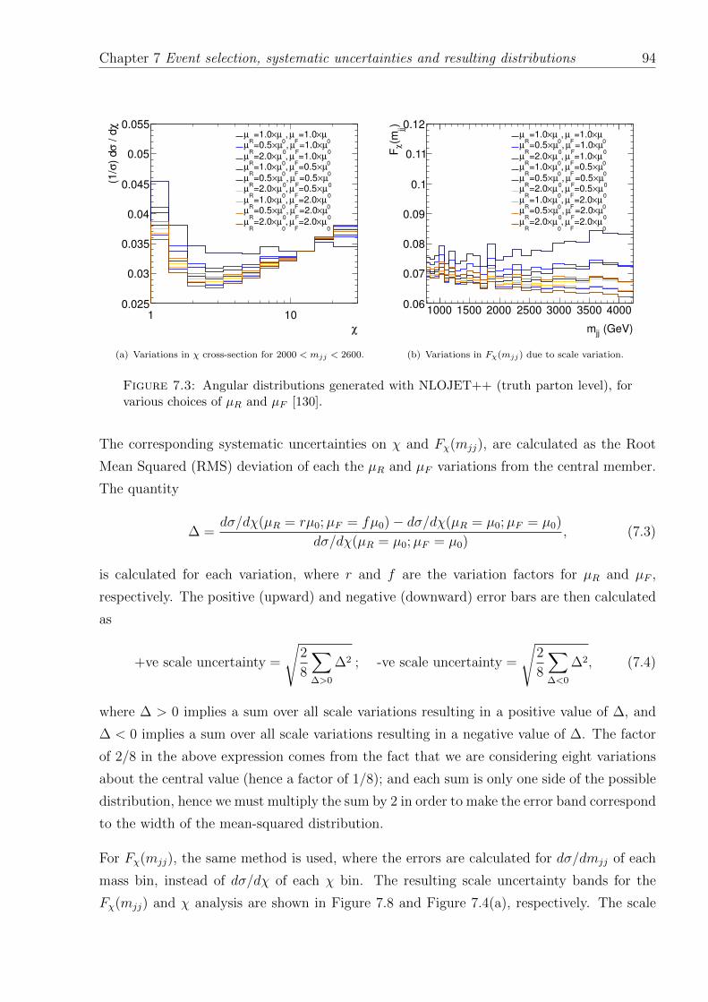
Chapter 7 Event selection, systematic uncertainties and resulting distributions 94
χ
1 10
χ /
dσ
) d
σ(1
/
0.025
0.03
0.035
0.04
0.045
0.05
0.055
0µ×=1.0
Fµ,
0µ×=1.0
Rµ
0µ×=1.0
Fµ,
0µ×=0.5
Rµ
0µ×=1.0
Fµ,
0µ×=2.0
Rµ
0µ×=0.5
Fµ,
0µ×=1.0
Rµ
0µ×=0.5
Fµ,
0µ×=0.5
Rµ
0µ×=0.5
Fµ,
0µ×=2.0
Rµ
0µ×=2.0
Fµ,
0µ×=1.0
Rµ
0µ×=2.0
Fµ,
0µ×=0.5
Rµ
0µ×=2.0
Fµ,
0µ×=2.0
Rµ
(a) Variations in χ cross-section for 2000 < mjj < 2600.
(GeV)jjm
1000 1500 2000 2500 3000 3500 4000
)jj
(mχ
F
0.06
0.07
0.08
0.09
0.1
0.11
0.12
0µ×=1.0
Fµ,
0µ×=1.0
Rµ
0µ×=1.0
Fµ,
0µ×=0.5
Rµ
0µ×=1.0
Fµ,
0µ×=2.0
Rµ
0µ×=0.5
Fµ,
0µ×=1.0
Rµ
0µ×=0.5
Fµ,
0µ×=0.5
Rµ
0µ×=0.5
Fµ,
0µ×=2.0
Rµ
0µ×=2.0
Fµ,
0µ×=1.0
Rµ
0µ×=2.0
Fµ,
0µ×=0.5
Rµ
0µ×=2.0
Fµ,
0µ×=2.0
Rµ
(b) Variations in Fχ(mjj) due to scale variation.
Figure 7.3: Angular distributions generated with NLOJET++ (truth parton level), forvarious choices of µR and µF [130].
The corresponding systematic uncertainties on χ and Fχ(mjj), are calculated as the Root
Mean Squared (RMS) deviation of each the µR and µF variations from the central member.
The quantity
∆ =dσ/dχ(µR = rµ0;µF = fµ0)− dσ/dχ(µR = µ0;µF = µ0)
dσ/dχ(µR = µ0;µF = µ0), (7.3)
is calculated for each variation, where r and f are the variation factors for µR and µF ,
respectively. The positive (upward) and negative (downward) error bars are then calculated
as
+ve scale uncertainty =
√2
8
∑∆>0
∆2 ; -ve scale uncertainty =
√2
8
∑∆<0
∆2, (7.4)
where ∆ > 0 implies a sum over all scale variations resulting in a positive value of ∆, and
∆ < 0 implies a sum over all scale variations resulting in a negative value of ∆. The factor
of 2/8 in the above expression comes from the fact that we are considering eight variations
about the central value (hence a factor of 1/8); and each sum is only one side of the possible
distribution, hence we must multiply the sum by 2 in order to make the error band correspond
to the width of the mean-squared distribution.
For Fχ(mjj), the same method is used, where the errors are calculated for dσ/dmjj of each
mass bin, instead of dσ/dχ of each χ bin. The resulting scale uncertainty bands for the
Fχ(mjj) and χ analysis are shown in Figure 7.8 and Figure 7.4(a), respectively. The scale
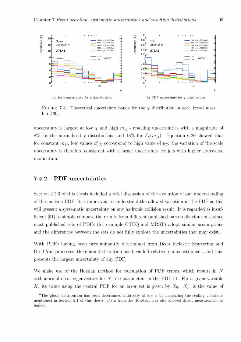
Chapter 7 Event selection, systematic uncertainties and resulting distributions 95
χ1 10
Uncertainty (%)
0
2
4
6
8
10
12
14< 7000 GeV
jj2600 < m
< 2600 GeVjj
2000 < m
< 2000 GeVjj
1600 < m
< 1600 GeVjj
1200 < m
< 1200 GeVjj
800 < m
σ+ 1
σ- 1
ATLAS
Scaleuncertainty
=7 TeVs
(a) Scale uncertainty for χ distributions
!1 10
Unc
erta
inty
(%)
0
0.2
0.4
0.6
0.8
1
1.2
1.4
1.6
1.8
2
< 7000 GeVjj2600 < m< 2600 GeVjj2000 < m< 2000 GeVjj1600 < m< 1600 GeVjj1200 < m
< 1200 GeVjj800 < m
"+ 1
"- 1
ATLAS
PDFuncertainty
=7 TeVs
(b) PDF uncertainty for χ distributions
Figure 7.4: Theoretical uncertainty bands for the χ distribution in each broad massbin [130].
uncertainty is largest at low χ and high mjj - reaching uncertainties with a magnitude of
8% for the normalised χ distributions and 18% for Fχ(mjj). Equation 6.20 showed that
for constant mjj, low values of χ correspond to high value of pT : the variation of the scale
uncertainty is therefore consistent with a larger uncertainty for jets with higher transverse
momentum.
7.4.2 PDF uncertainties
Section 2.2.3 of this thesis included a brief discussion of the evolution of our understanding
of the nucleon PDF. It is important to understand the allowed variation in the PDF as this
will present a systematic uncertainty on any hadronic collision result. It is regarded as insuf-
ficient [51] to simply compare the results from different published parton distributions, since
most published sets of PDFs (for example CTEQ and MRST) adopt similar assumptions
and the differences between the sets do not fully explore the uncertainties that may exist.
With PDFs having been predominantly determined from Deep Inelastic Scattering and
Drell-Yan processes, the gluon distribution has been left relatively unconstrained6, and thus
presents the largest uncertainty of any PDF.
We make use of the Hessian method for calculation of PDF errors, which results in N
orthonormal error eigenvectors for N free parameters in the PDF fit. For a given variable
X, its value using the central PDF for an error set is given by X0. X+i is the value of
6The gluon distribution has been determined indirectly at low x by measuring the scaling violationsmentioned in Section 2.1 of this thesis. Data from the Tevatron has also allowed direct measurement athigh-x.
Chapter 7 Event selection, systematic uncertainties and resulting distributions 96
that variable using the PDF corresponding to the “+” direction for eigenvector i and X−i
is the value for the variable using the PDF corresponding to the “-” direction. The Master
Equation is then used to calculate the total PDF error [51]:
∆X+max =
√√√√ N∑i=1
[max(X+i −X0, X
−i −X0, 0)]2
∆X−max =
√√√√ N∑i=1
[max(X0 −X+i , X0 −X−i , 0)]2. (7.5)
The +ve and -ve components may be added in quadrature, since the PDF eigenvectors form
an orthonormal basis. We use NLOJET++ connected to APPLgrid with the CT10 error
members.
The resulting +ve and -ve PDF errors for Fχ(mjj) are shown in Figure 7.8 and are included
in Table 7.7. The PDF uncertainty on Fχ is seen to increase with mjj, ranging from 0.33%
to 3.25%. PDF uncertainties are expected to increase with the invariant mass of the dijet
system, since these events will tend to be produced in collisions involving partons with higher
values of Bjorken-x, where the PDF uncertainty increases.
The resulting PDF uncertainties for χ are shown in Figure 7.4(b) and are included in Ta-
ble 7.8. The size of the systematic uncertainty is found to range from being negligible to
a maximum of 1.06%, with the largest uncertainty occuring at low χ, corrsponding to high
jet momentum. This is consistent with the discussion of the PDF uncertainties for Fχ(mjj),
where the uncertainty increases with the Bjorken-x of the interacting partons.
7.5 Experimental systematic uncertainties
7.5.1 Jet energy scale uncertainties
JES Pseudo-Experiments (PEs) obtained from MC have been used for the derivation of
the JES uncertainty. This is typically done by running over the MC samples 1000 times,
each time varying the JES of all jets in all events according to the uncertainty given by the
JESUncertaintyProvider. The JESUncertaintyProvider [121] is introduced in Section 5.5.1.
The 14 nuisance parameter configuration is used and it is assumed that the uncertainties on
jet energies have a Gaussian distribution. This means that each PE has a set of 14 random
numbers drawn from a Gaussian with zero mean and σ = 1. For PE i each jet ijet is then
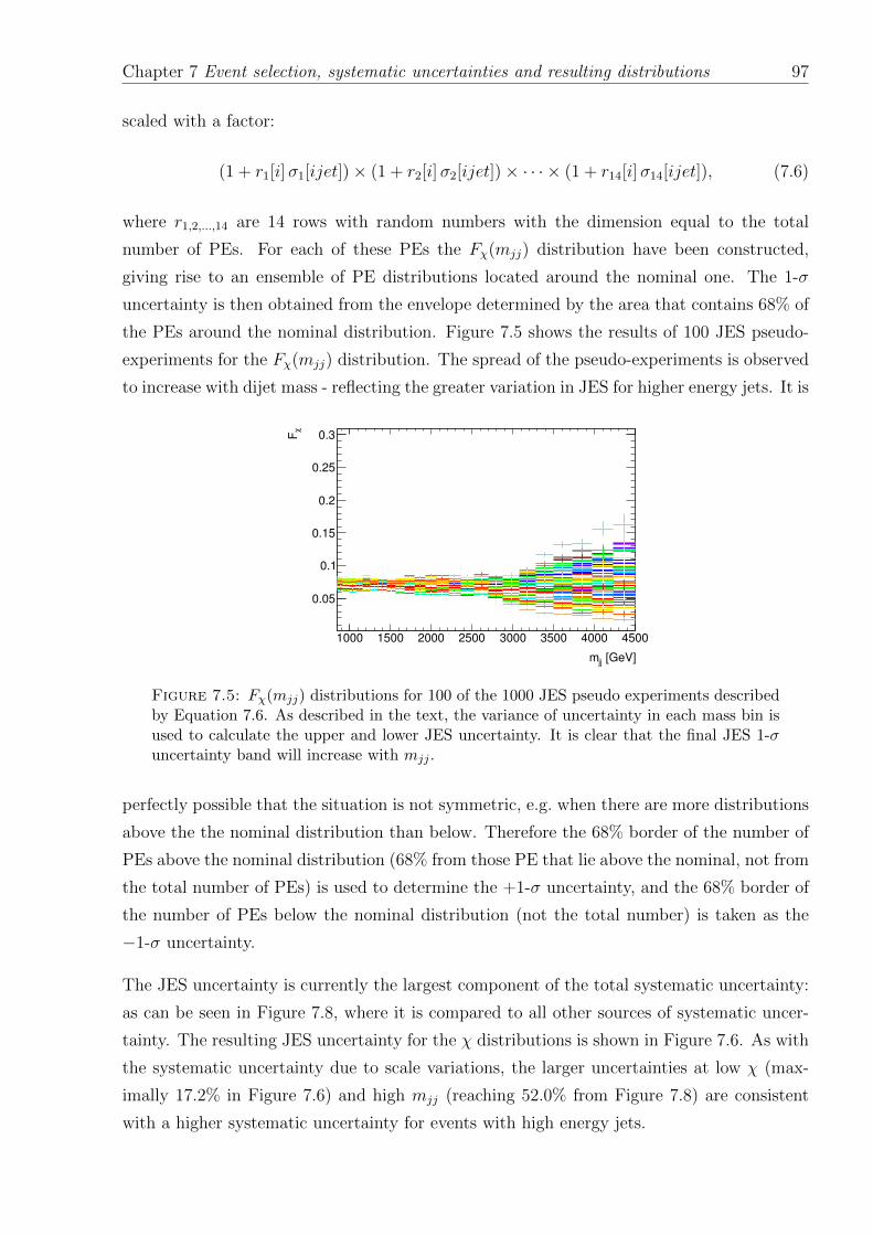
Chapter 7 Event selection, systematic uncertainties and resulting distributions 97
scaled with a factor:
(1 + r1[i]σ1[ijet])× (1 + r2[i]σ2[ijet])× · · · × (1 + r14[i]σ14[ijet]), (7.6)
where r1,2,...,14 are 14 rows with random numbers with the dimension equal to the total
number of PEs. For each of these PEs the Fχ(mjj) distribution have been constructed,
giving rise to an ensemble of PE distributions located around the nominal one. The 1-σ
uncertainty is then obtained from the envelope determined by the area that contains 68% of
the PEs around the nominal distribution. Figure 7.5 shows the results of 100 JES pseudo-
experiments for the Fχ(mjj) distribution. The spread of the pseudo-experiments is observed
to increase with dijet mass - reflecting the greater variation in JES for higher energy jets. It is
[GeV]jjm
1000 1500 2000 2500 3000 3500 4000 4500
χF
0.05
0.1
0.15
0.2
0.25
0.3
Figure 7.5: Fχ(mjj) distributions for 100 of the 1000 JES pseudo experiments describedby Equation 7.6. As described in the text, the variance of uncertainty in each mass bin isused to calculate the upper and lower JES uncertainty. It is clear that the final JES 1-σuncertainty band will increase with mjj .
perfectly possible that the situation is not symmetric, e.g. when there are more distributions
above the the nominal distribution than below. Therefore the 68% border of the number of
PEs above the nominal distribution (68% from those PE that lie above the nominal, not from
the total number of PEs) is used to determine the +1-σ uncertainty, and the 68% border of
the number of PEs below the nominal distribution (not the total number) is taken as the
−1-σ uncertainty.
The JES uncertainty is currently the largest component of the total systematic uncertainty:
as can be seen in Figure 7.8, where it is compared to all other sources of systematic uncer-
tainty. The resulting JES uncertainty for the χ distributions is shown in Figure 7.6. As with
the systematic uncertainty due to scale variations, the larger uncertainties at low χ (max-
imally 17.2% in Figure 7.6) and high mjj (reaching 52.0% from Figure 7.8) are consistent
with a higher systematic uncertainty for events with high energy jets.
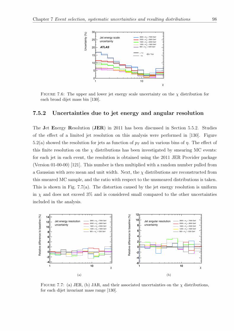
Chapter 7 Event selection, systematic uncertainties and resulting distributions 98
χ1 10
Un
ce
rta
inty
(%
)
0
5
10
15
20
25
30
< 7000 GeVjj
2600 < m
< 2600 GeVjj
2000 < m
< 2000 GeVjj
1600 < m
< 1600 GeVjj
1200 < m
< 1200 GeVjj
800 < m
σ+ 1
σ- 1
ATLAS
Jet energy scale
uncertainty
=7 TeVs
Figure 7.6: The upper and lower jet energy scale uncertainty on the χ distribution foreach broad dijet mass bin [130].
7.5.2 Uncertainties due to jet energy and angular resolution
The Jet Energy Resolution (JER) in 2011 has been discussed in Section 5.5.2. Studies
of the effect of a limited jet resolution on this analysis were performed in [130]. Figure
5.2(a) showed the resolution for jets as function of pT and in various bins of η. The effect of
this finite resolution on the χ distributions has been investigated by smearing MC events:
for each jet in each event, the resolution is obtained using the 2011 JER Provider package
(Version 01-00-00) [121]. This number is then multiplied with a random number pulled from
a Gaussian with zero mean and unit width. Next, the χ distributions are reconstructed from
this smeared MC sample, and the ratio with respect to the unsmeared distributions is taken.
This is shown in Fig. 7.7(a). The distortion caused by the jet energy resolution is uniform
in χ and does not exceed 3% and is considered small compared to the other uncertainties
included in the analysis.
χ1 10
Re
lative
diffe
ren
ce
to
baselin
e (
%)
4
2
0
2
4
6
8
10
12
14
1 10
4
2
0
2
4
6
8
10
12
14 < 7000 GeV
jj2600 < m
< 2600 GeVjj
2000 < m
< 2000 GeVjj
1600 < m
< 1600 GeVjj
1200 < m
< 1200 GeVjj
800 < m
Jet energy resolution
uncertainty
(a)
χ1 10
Re
lative
diffe
ren
ce
to
baselin
e (
%)
6
4
2
0
2
4
6
8
10
12
1 106
4
2
0
2
4
6
8
10
12
< 7000 GeVjj
2600 < m
< 2600 GeVjj
2000 < m
< 2000 GeVjj
1600 < m
< 1600 GeVjj
1200 < m
< 1200 GeVjj
800 < m
Jet angular resolution
uncertainty
(b)
Figure 7.7: (a) JER, (b) JAR, and their associated uncertainties on the χ distributions,for each dijet invariant mass range [130].
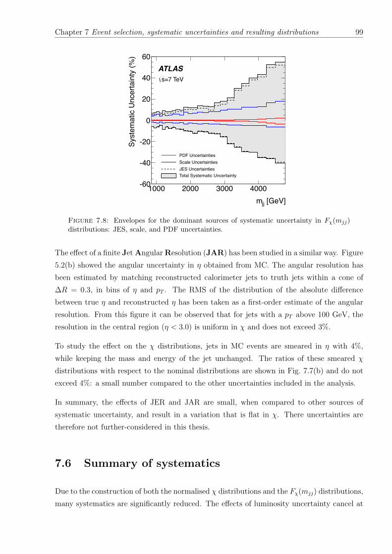
Chapter 7 Event selection, systematic uncertainties and resulting distributions 99
[GeV]jjm1000 2000 3000 4000
Syst
emat
ic U
ncer
tain
ty (%
)
-60
-40
-20
0
20
40
60
PDF UncertaintiesScale UncertaintiesJES UncertaintiesTotal Systematic Uncertainty
ATLAS=7 TeVs
Figure 7.8: Envelopes for the dominant sources of systematic uncertainty in Fχ(mjj)distributions: JES, scale, and PDF uncertainties.
The effect of a finite Jet Angular Resolution (JAR) has been studied in a similar way. Figure
5.2(b) showed the angular uncertainty in η obtained from MC. The angular resolution has
been estimated by matching reconstructed calorimeter jets to truth jets within a cone of
∆R = 0.3, in bins of η and pT . The RMS of the distribution of the absolute difference
between true η and reconstructed η has been taken as a first-order estimate of the angular
resolution. From this figure it can be observed that for jets with a pT above 100 GeV, the
resolution in the central region (η < 3.0) is uniform in χ and does not exceed 3%.
To study the effect on the χ distributions, jets in MC events are smeared in η with 4%,
while keeping the mass and energy of the jet unchanged. The ratios of these smeared χ
distributions with respect to the nominal distributions are shown in Fig. 7.7(b) and do not
exceed 4%: a small number compared to the other uncertainties included in the analysis.
In summary, the effects of JER and JAR are small, when compared to other sources of
systematic uncertainty, and result in a variation that is flat in χ. There uncertainties are
therefore not further-considered in this thesis.
7.6 Summary of systematics
Due to the construction of both the normalised χ distributions and the Fχ(mjj) distributions,
many systematics are significantly reduced. The effects of luminosity uncertainty cancel at
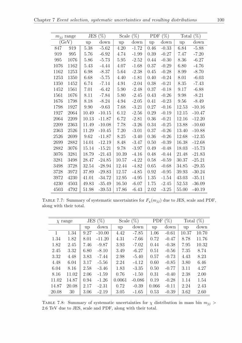
Chapter 7 Event selection, systematic uncertainties and resulting distributions 100
mjj range JES (%) Scale (%) PDF (%) Total (%)(GeV) up down up down up down up down
847 919 5.38 -5.62 4.20 -1.72 0.46 -0.33 6.84 -5.88919 995 5.76 -6.92 4.74 -1.99 0.39 -0.27 7.47 -7.20995 1076 5.86 -5.73 5.95 -2.52 0.44 -0.30 8.36 -6.271076 1162 5.43 -4.44 4.07 -1.68 0.37 -0.29 6.80 -4.761162 1253 6.98 -8.37 5.64 -2.38 0.45 -0.28 8.99 -8.701253 1350 6.68 -5.75 4.40 -1.81 0.40 -0.24 8.01 -6.031350 1452 6.74 -7.14 4.91 -2.04 0.38 -0.21 8.35 -7.431452 1561 7.01 -6.42 5.90 -2.48 0.37 -0.18 9.17 -6.881561 1676 8.11 -7.84 5.80 -2.45 0.43 -0.26 9.98 -8.211676 1798 8.18 -8.24 4.94 -2.05 0.41 -0.23 9.56 -8.491798 1927 9.90 -9.63 7.68 -3.21 0.27 -0.16 12.53 -10.161927 2064 10.49 -10.15 6.12 -2.56 0.29 -0.19 12.15 -10.472064 2209 10.13 -11.87 6.72 -2.81 0.36 -0.21 12.16 -12.202209 2363 11.49 -10.08 7.78 -3.26 0.34 -0.25 13.88 -10.602363 2526 11.29 -10.45 7.20 -3.01 0.37 -0.26 13.40 -10.882526 2699 9.62 -11.87 8.25 -3.40 0.36 -0.26 12.68 -12.352699 2882 14.01 -12.19 8.48 -3.47 0.50 -0.39 16.38 -12.682882 3076 15.14 -15.21 9.78 -3.97 0.49 -0.48 18.03 -15.733076 3281 18.79 -21.43 10.39 -4.16 0.48 -0.44 21.48 -21.833281 3498 28.47 -24.85 10.57 -4.22 0.58 -0.59 30.37 -25.213498 3728 32.54 -28.94 12.44 -4.82 0.65 -0.68 34.85 -29.353728 3972 37.89 -29.83 12.57 -4.85 0.92 -0.95 39.93 -30.243972 4230 41.01 -34.72 12.95 -4.95 1.35 -1.54 43.03 -35.114230 4503 49.83 -35.49 16.50 -6.07 1.75 -2.45 52.53 -36.094503 4792 51.98 -39.53 17.86 -6.43 2.02 -3.25 55.00 -40.19
Table 7.7: Summary of systematic uncertainties for Fχ(mjj) due to JES, scale and PDF,along with their total.
χ range JES (%) Scale (%) PDF (%) Total (%)up down up down up down up down
1 1.34 9.27 -10.00 4.42 -7.85 1.06 -0.61 10.37 10.701.34 1.82 8.01 -11.20 4.31 -7.66 0.72 -0.47 8.78 11.761.82 2.45 7.46 -9.87 3.93 -7.02 0.44 -0.38 7.95 10.322.45 3.32 6.80 -8.10 3.49 -6.27 0.51 -0.56 7.35 8.743.32 4.48 3.83 -7.44 2.98 -5.40 0.57 -0.73 4.43 8.234.48 6.04 3.17 -5.56 2.24 -4.12 0.60 -0.85 3.80 6.466.04 8.16 2.58 -3.46 1.83 -3.35 0.50 -0.77 3.11 4.278.16 11.02 2.06 -1.59 0.76 -1.50 0.31 -0.40 2.38 2.0011.02 14.87 0.94 -1.26 0.0061 -0.086 0.19 -0.28 1.14 1.5414.87 20.08 2.17 -2.31 0.72 -0.39 0.066 -0.11 2.24 2.4320.08 30 3.06 -2.19 3.05 -1.65 0.53 -0.39 3.62 2.60
Table 7.8: Summary of systematic uncertainties for χ distribution in mass bin mjj >2.6 TeV due to JES, scale and PDF, along with their total.
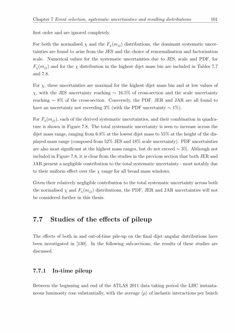
Chapter 7 Event selection, systematic uncertainties and resulting distributions 101
first order and are ignored completely.
For both the normalised χ and the Fχ(mjj) distributions, the dominant systematic uncer-
tainties are found to arise from the JES and the choice of renormalisation and factorisation
scale. Numerical values for the systematic uncertainties due to JES, scale and PDF, for
Fχ(mjj) and for the χ distribution in the highest dijet mass bin are included in Tables 7.7
and 7.8.
For χ, these uncertainties are maximal for the highest dijet mass bin and at low values of
χ, with the JES uncertainty reaching ∼ 16.5% of cross-section and the scale uncertainty
reaching ∼ 8% of the cross-section. Conversely, the PDF, JER and JAR are all found to
have an uncertainty not exceeding 3% (with the PDF uncertainty ∼ 1%).
For Fχ(mjj), each of the derived systematic uncertainties, and their combination in quadra-
ture is shown in Figure 7.8. The total systematic uncertainty is seen to increase across the
dijet mass range, ranging from 6.8% at the lowest dijet mass to 55% at the height of the dis-
played mass range (composed from 52% JES and 18% scale uncertainty). PDF uncertainties
are also most significant at the highest mass ranges, but do not exceed ∼ 3%. Although not
included in Figure 7.8, it is clear from the studies in the previous section that both JER and
JAR present a negligible contribution to the total systematic uncertainty - most notably due
to their uniform effect over the χ range for all broad mass windows.
Given their relatively negligible contribution to the total systematic uncertainty across both
the normalised χ and Fχ(mjj) distributions, the PDF, JER and JAR uncertainties will not
be considered further in this thesis.
7.7 Studies of the effects of pileup
The effects of both in and out-of-time pile-up on the final dijet angular distributions have
been investigated in [130]. In the following sub-sections, the results of these studies are
discussed.
7.7.1 In-time pileup
Between the beginning and end of the ATLAS 2011 data taking period the LHC instanta-
neous luminosity rose substantially, with the average 〈µ〉 of inelastic interactions per bunch
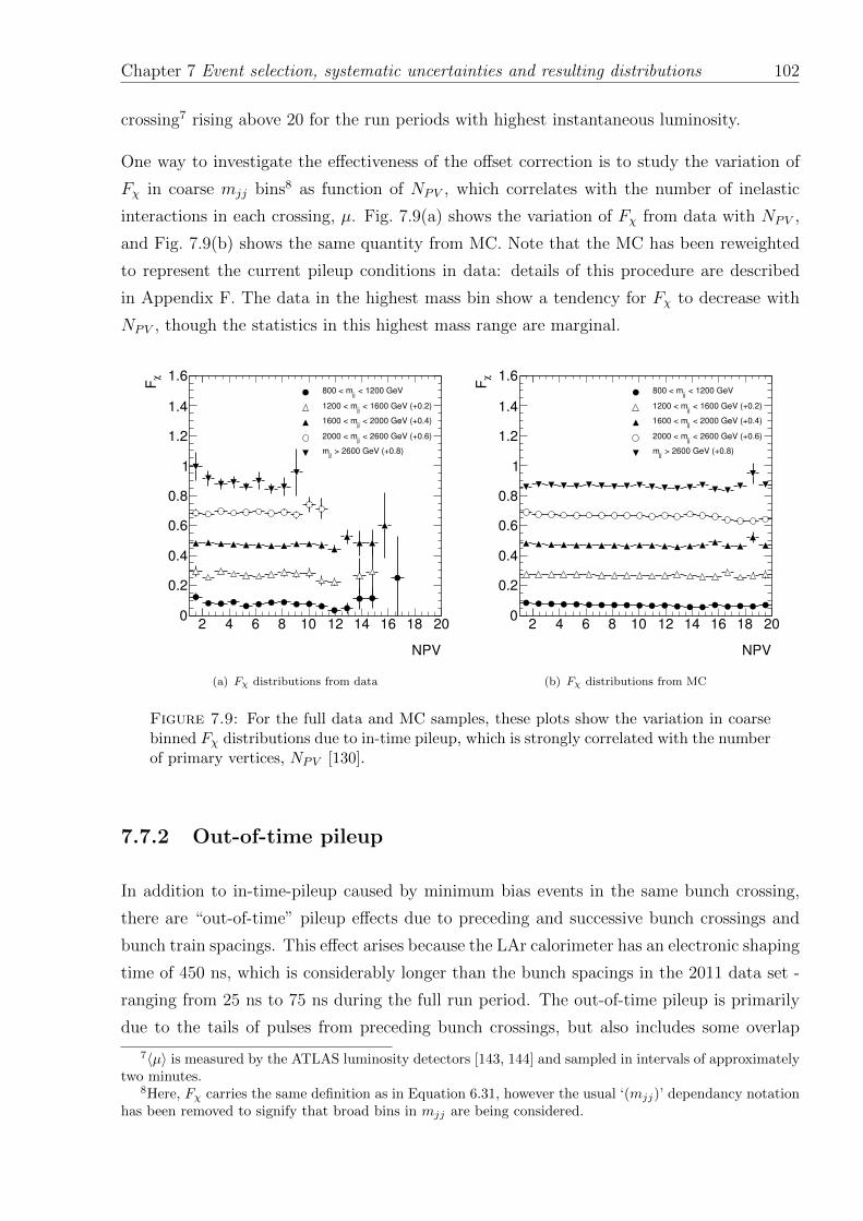
Chapter 7 Event selection, systematic uncertainties and resulting distributions 102
crossing7 rising above 20 for the run periods with highest instantaneous luminosity.
One way to investigate the effectiveness of the offset correction is to study the variation of
Fχ in coarse mjj bins8 as function of NPV , which correlates with the number of inelastic
interactions in each crossing, µ. Fig. 7.9(a) shows the variation of Fχ from data with NPV ,
and Fig. 7.9(b) shows the same quantity from MC. Note that the MC has been reweighted
to represent the current pileup conditions in data: details of this procedure are described
in Appendix F. The data in the highest mass bin show a tendency for Fχ to decrease with
NPV , though the statistics in this highest mass range are marginal.
NPV
2 4 6 8 10 12 14 16 18 20
χF
0
0.2
0.4
0.6
0.8
1
1.2
1.4
1.6 < 1200 GeV
jj800 < m
< 1600 GeV (+0.2)jj
1200 < m
< 2000 GeV (+0.4)jj
1600 < m
< 2600 GeV (+0.6)jj
2000 < m
> 2600 GeV (+0.8)jj
m
(a) Fχ distributions from data
NPV
2 4 6 8 10 12 14 16 18 20
χF
0
0.2
0.4
0.6
0.8
1
1.2
1.4
1.6 < 1200 GeV
jj800 < m
< 1600 GeV (+0.2)jj
1200 < m
< 2000 GeV (+0.4)jj
1600 < m
< 2600 GeV (+0.6)jj
2000 < m
> 2600 GeV (+0.8)jj
m
(b) Fχ distributions from MC
Figure 7.9: For the full data and MC samples, these plots show the variation in coarsebinned Fχ distributions due to in-time pileup, which is strongly correlated with the numberof primary vertices, NPV [130].
7.7.2 Out-of-time pileup
In addition to in-time-pileup caused by minimum bias events in the same bunch crossing,
there are “out-of-time” pileup effects due to preceding and successive bunch crossings and
bunch train spacings. This effect arises because the LAr calorimeter has an electronic shaping
time of 450 ns, which is considerably longer than the bunch spacings in the 2011 data set -
ranging from 25 ns to 75 ns during the full run period. The out-of-time pileup is primarily
due to the tails of pulses from preceding bunch crossings, but also includes some overlap
7〈µ〉 is measured by the ATLAS luminosity detectors [143, 144] and sampled in intervals of approximatelytwo minutes.
8Here, Fχ carries the same definition as in Equation 6.31, however the usual ‘(mjj)’ dependancy notationhas been removed to signify that broad bins in mjj are being considered.
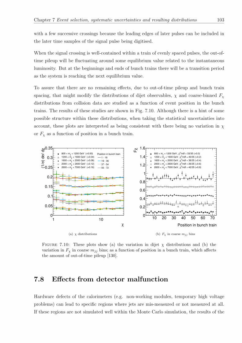
Chapter 7 Event selection, systematic uncertainties and resulting distributions 103
with a few successive crossings because the leading edges of later pulses can be included in
the later time samples of the signal pulse being digitised.
When the signal crossing is well-contained within a train of evenly spaced pulses, the out-of-
time pileup will be fluctuating around some equilibrium value related to the instantaneous
luminosity. But at the beginnings and ends of bunch trains there will be a transition period
as the system is reaching the next equilibrium value.
To assure that there are no remaining effects, due to out-of-time pileup and bunch train
spacing, that might modify the distributions of dijet observables, χ and coarse-binned Fχ
distributions from collision data are studied as a function of event position in the bunch
trains. The results of these studies are shown in Fig. 7.10. Although there is a hint of some
possible structure within these distributions, when taking the statistical uncertainties into
account, these plots are interpreted as being consistent with there being no variation in χ
or Fχ as a function of position in a bunch train.
χ
1 10
χ/ d
σ)
dσ
(1/
0
0.05
0.1
0.15
0.2
0.25
0.3
0.35
< 1200 GeV (+0.00)jj
800 < m
< 1600 GeV (+0.04)jj
1200 < m
< 2000 GeV (+0.08)jj
1600 < m
< 2600 GeV (+0.12)jj
2000 < m
< 7000 GeV (+0.16)jj
2600 < m
Position in bunch train
1 18
19 36
37 54
55 72
(a) χ distributions
Position in bunch train
10 20 30 40 50 60 70
χF
0
0.2
0.4
0.6
0.8
1
1.2
1.4
1.6
/ndf = 33/35 (+0.0)2χ < 1200 GeV ,
jj800 < m
/ndf = 40/35 (+0.2)2χ < 1600 GeV ,
jj1200 < m
/ndf = 38/35 (+0.4)2χ < 2000 GeV ,
jj1600 < m
/ndf = 26/35 (+0.6)2χ < 2600 GeV ,
jj2000 < m
/ndf = 42/35 (+0.8)2χ < 7000 GeV ,
jj2600 < m
(b) Fχ in coarse mjj bins
Figure 7.10: These plots show (a) the variation in dijet χ distributions and (b) thevariation in Fχ in coarse mjj bins; as a function of position in a bunch train, which affectsthe amount of out-of-time pileup [130].
7.8 Effects from detector malfunction
Hardware defects of the calorimeters (e.g. non-working modules, temporary high voltage
problems) can lead to specific regions where jets are mis-measured or not measured at all.
If these regions are not simulated well within the Monte Carlo simulation, the results of the
Chapter 7 Event selection, systematic uncertainties and resulting distributions 104
angular analyses can be affected because the defects will lead to different jet rates in different
pseudorapidity regions.
Permanently dead regions in the calorimeter could affect the measured distributions. In
the case of a dead tile calorimeter cell, a correction is applied to its raw energy scale. The
correction factor 1.0−BCH CORR CELL is equal to the sum of the energies in the corrected
cells neighbouring this cell divided by their total energy, and is applied such that
Eraw, corrected =Eraw, uncorrected
(1.0− BCH CORR CELL). (7.7)
This correction is done by default in the reconstruction.
An improved correction can be applied at the jet level: BCH CORR JET equals the sum of
the estimation for bad cells in the jet cone divided by the total energy. The total correction
is then given by
Ejet-level corrected = Eraw, corrected(1.0− BCH CORR CELL)
(1.0− BCH CORR JET). (7.8)
The above formula cancels the default cell-based correction step and applies the new cor-
rection at the jet level. It is applied to the jet energy at the EM-scale before applying a
hadronic calibration. Performance studies have shown that the “jet-level” correction per-
forms better in jet closure tests [121] and therefore we have used it through the entire dijet
analysis. Figure 7.11 shows the distribution of correction factors for data events that have
a fully reconstructed dijet mass above 700 GeV.
(1 bch_corr_cell) / (1 bch_corr_jet)
0.9 0.95 1 1.05 1.1
jets
N
410
510
610
710
Figure 7.11: Distribution of the bad tile channel correction factor for data events withdijet mass above 700 GeV [130].
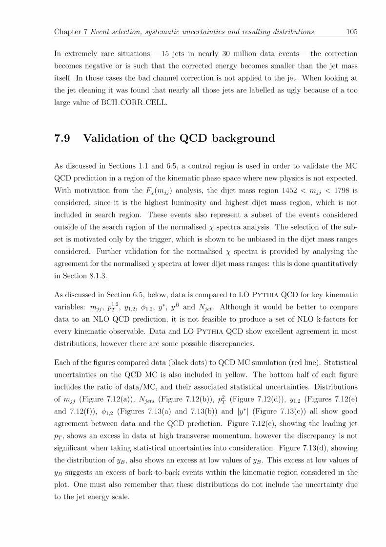
Chapter 7 Event selection, systematic uncertainties and resulting distributions 105
In extremely rare situations —15 jets in nearly 30 million data events— the correction
becomes negative or is such that the corrected energy becomes smaller than the jet mass
itself. In those cases the bad channel correction is not applied to the jet. When looking at
the jet cleaning it was found that nearly all those jets are labelled as ugly because of a too
large value of BCH CORR CELL.
7.9 Validation of the QCD background
As discussed in Sections 1.1 and 6.5, a control region is used in order to validate the MC
QCD prediction in a region of the kinematic phase space where new physics is not expected.
With motivation from the Fχ(mjj) analysis, the dijet mass region 1452 < mjj < 1798 is
considered, since it is the highest luminosity and highest dijet mass region, which is not
included in search region. These events also represent a subset of the events considered
outside of the search region of the normalised χ spectra analysis. The selection of the sub-
set is motivated only by the trigger, which is shown to be unbiased in the dijet mass ranges
considered. Further validation for the normalised χ spectra is provided by analysing the
agreement for the normalised χ spectra at lower dijet mass ranges: this is done quantitatively
in Section 8.1.3.
As discussed in Section 6.5, below, data is compared to LO Pythia QCD for key kinematic
variables: mjj, p1,2T , y1,2, φ1,2, y∗, yB and Njet. Although it would be better to compare
data to an NLO QCD prediction, it is not feasible to produce a set of NLO k-factors for
every kinematic observable. Data and LO Pythia QCD show excellent agreement in most
distributions, however there are some possible discrepancies.
Each of the figures compared data (black dots) to QCD MC simulation (red line). Statistical
uncertainties on the QCD MC is also included in yellow. The bottom half of each figure
includes the ratio of data/MC, and their associated statistical uncertainties. Distributions
of mjj (Figure 7.12(a)), Njets (Figure 7.12(b)), p2T (Figure 7.12(d)), y1,2 (Figures 7.12(e)
and 7.12(f)), φ1,2 (Figures 7.13(a) and 7.13(b)) and |y∗| (Figure 7.13(c)) all show good
agreement between data and the QCD prediction. Figure 7.12(c), showing the leading jet
pT , shows an excess in data at high transverse momentum, however the discrepancy is not
significant when taking statistical uncertainties into consideration. Figure 7.13(d), showing
the distribution of yB, also shows an excess at low values of yB. This excess at low values of
yB suggests an excess of back-to-back events within the kinematic region considered in the
plot. One must also remember that these distributions do not include the uncertainty due
to the jet energy scale.
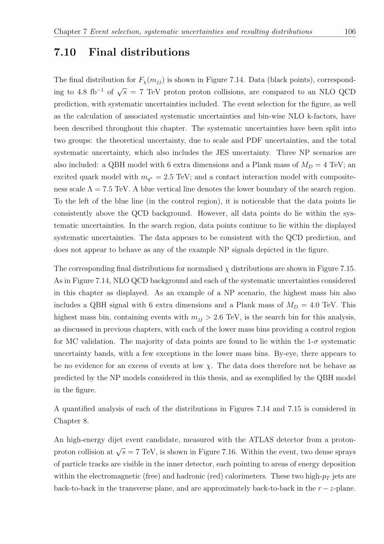
Chapter 7 Event selection, systematic uncertainties and resulting distributions 106
7.10 Final distributions
The final distribution for Fχ(mjj) is shown in Figure 7.14. Data (black points), correspond-
ing to 4.8 fb−1 of√s = 7 TeV proton proton collisions, are compared to an NLO QCD
prediction, with systematic uncertainties included. The event selection for the figure, as well
as the calculation of associated systematic uncertainties and bin-wise NLO k-factors, have
been described throughout this chapter. The systematic uncertainties have been split into
two groups: the theoretical uncertainty, due to scale and PDF uncertainties, and the total
systematic uncertainty, which also includes the JES uncertainty. Three NP scenarios are
also included: a QBH model with 6 extra dimensions and a Plank mass of MD = 4 TeV; an
excited quark model with mq∗ = 2.5 TeV; and a contact interaction model with composite-
ness scale Λ = 7.5 TeV. A blue vertical line denotes the lower boundary of the search region.
To the left of the blue line (in the control region), it is noticeable that the data points lie
consistently above the QCD background. However, all data points do lie within the sys-
tematic uncertainties. In the search region, data points continue to lie within the displayed
systematic uncertainties. The data appears to be consistent with the QCD prediction, and
does not appear to behave as any of the example NP signals depicted in the figure.
The corresponding final distributions for normalised χ distributions are shown in Figure 7.15.
As in Figure 7.14, NLO QCD background and each of the systematic uncertainties considered
in this chapter as displayed. As an example of a NP scenario, the highest mass bin also
includes a QBH signal with 6 extra dimensions and a Plank mass of MD = 4.0 TeV. This
highest mass bin, containing events with mjj > 2.6 TeV, is the search bin for this analysis,
as discussed in previous chapters, with each of the lower mass bins providing a control region
for MC validation. The majority of data points are found to lie within the 1-σ systematic
uncertainty bands, with a few exceptions in the lower mass bins. By-eye, there appears to
be no evidence for an excess of events at low χ. The data does therefore not be behave as
predicted by the NP models considered in this thesis, and as exemplified by the QBH model
in the figure.
A quantified analysis of each of the distributions in Figures 7.14 and 7.15 is considered in
Chapter 8.
An high-energy dijet event candidate, measured with the ATLAS detector from a proton-
proton collision at√s = 7 TeV, is shown in Figure 7.16. Within the event, two dense sprays
of particle tracks are visible in the inner detector, each pointing to areas of energy deposition
within the electromagnetic (free) and hadronic (red) calorimeters. These two high-pT jets are
back-to-back in the transverse plane, and are approximately back-to-back in the r−z-plane.
Chapter 7 Event selection, systematic uncertainties and resulting distributions 107
[GeV]jjm
Eve
nts
1
10
210
310
410
510
610
7101
L dt = 4.8 fb∫Data
QCD Prediction (Pythia LO*)
< 1798 GeVjj
1452 < m
[GeV]jjm
12001300140015001600 1700180019002000Data
/ M
C
00.5
11.5
2
(a) mjj
jetsN
Eve
nts
1
10
210
310
410
510
610
1 L dt = 4.8 fb∫Data
QCD Prediction (Pythia LO*)
< 1798 GeVjj
1452 < m
jetsN
0 2 4 6 8 10 12 14 16 18 20Data
/ M
C
00.5
11.5
2
(b) Njets
[GeV]T
Leading Jet p
Eve
nts
1
10
210
310
410
510
610
1 L dt = 4.8 fb∫Data
QCD Prediction (Pythia LO*)
< 1798 GeVjj
1452 < m
[GeV]T
Leading Jet p
0 200 400 600 800 1000 1200 1400Data
/ M
C
00.5
11.5
2
(c) pj1T
[GeV]T
Subleading Jet p
Eve
nts
1
10
210
310
410
510
610
1 L dt = 4.8 fb∫Data
QCD Prediction (Pythia LO*)
< 1798 GeVjj
1452 < m
[GeV]T
Subleading Jet p
0 200 400 600 800 1000 1200 1400Data
/ M
C
00.5
11.5
2
(d) pj2T
Leading Jet Rapidity
Eve
nts
0
1000
2000
3000
4000
5000
60001
L dt = 4.8 fb∫Data
QCD Prediction (Pythia LO*)
< 1798 GeVjj
1452 < m
Leading Jet Rapidity
3 2 1 0 1 2 3Data
/ M
C
00.5
11.5
2
(e) y1
Subleading Jet Rapidity
Eve
nts
0
1000
2000
3000
4000
5000
60001
L dt = 4.8 fb∫Data
QCD Prediction (Pythia LO*)
< 1798 GeVjj
1452 < m
Subleading Jet Rapidity
3 2 1 0 1 2 3Data
/ M
C
00.5
11.5
2
(f) y2
Figure 7.12: Data (black points) are compared to LO QCD (red line). Statistical uncer-tainties on the QCD MC are included in yellow.
Chapter 7 Event selection, systematic uncertainties and resulting distributions 108
φLeading Jet
Eve
nts
0
500
1000
1500
2000
2500
3000
35001
L dt = 4.8 fb∫Data
QCD Prediction (Pythia LO*)
< 1798 GeVjj
1452 < m
φLeading Jet
3 2 1 0 1 2 3Data
/ M
C
00.5
11.5
2
(a) φ1
φSubleading Jet E
ve
nts
0
500
1000
1500
2000
2500
3000
35001
L dt = 4.8 fb∫Data
QCD Prediction (Pythia LO*)
< 1798 GeVjj
1452 < m
φSubleading Jet
3 2 1 0 1 2 3Data
/ M
C
00.5
11.5
2
(b) φ2
|2
y1
|y
Eve
nts
0
2000
4000
6000
8000
10000
12000
14000
16000
18000
200001
L dt = 4.8 fb∫Data
QCD Prediction (Pythia LO*)
< 1798 GeVjj
1452 < m
|2
y1
|y
0 0.5 1 1.5 2 2.5 3 3.5 4Data
/ M
C
00.5
11.5
2
(c) |y∗| = |y1 − y2|
|2
+y1
|y
Eve
nts
0
2000
4000
6000
8000
10000
12000
14000 1 L dt = 4.8 fb∫Data
QCD Prediction (Pythia LO*)
< 1798 GeVjj
1452 < m
|2
+y1
|y
0 0.5 1 1.5 2 2.5Data
/ M
C
00.5
11.5
2
(d) |yB | = |y1 + y2|
Figure 7.13: Data (black points) are compared to LO QCD (red line). Statistical uncer-tainties on the QCD MC are included in yellow. The bottom half of each figure displaysthe ratio of data/MC, and their associated statistical uncertainties.
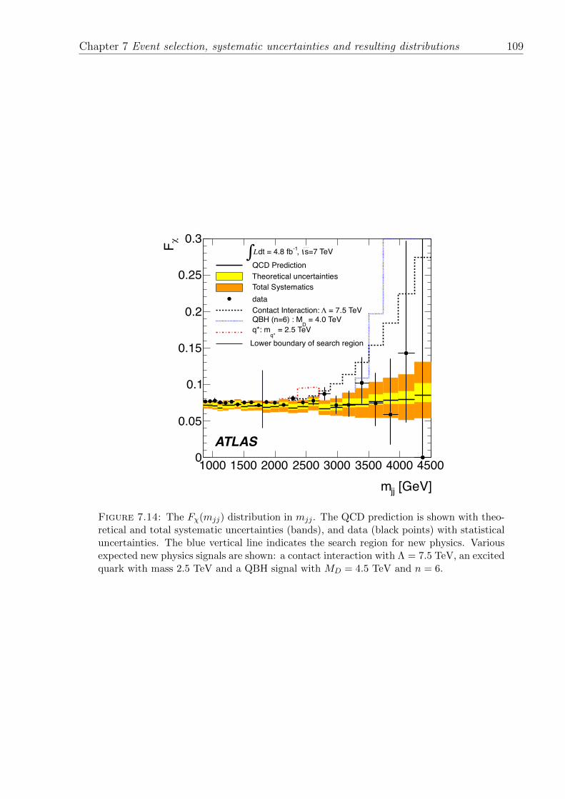
Chapter 7 Event selection, systematic uncertainties and resulting distributions 109
[GeV]jjm1000 1500 2000 2500 3000 3500 4000 4500
rF
0
0.05
0.1
0.15
0.2
0.25
0.3
ATLAS
=7 TeVs, -1dt = 4.8 fbL0 QCD Prediction Theoretical uncertainties Total Systematics data
= 7.5 TeVR Contact Interaction: = 4.0 TeV
D QBH (n=6) : M
= 2.5 TeVq*
q*: m Lower boundary of search region
Figure 7.14: The Fχ(mjj) distribution in mjj . The QCD prediction is shown with theo-retical and total systematic uncertainties (bands), and data (black points) with statisticaluncertainties. The blue vertical line indicates the search region for new physics. Variousexpected new physics signals are shown: a contact interaction with Λ = 7.5 TeV, an excitedquark with mass 2.5 TeV and a QBH signal with MD = 4.5 TeV and n = 6.
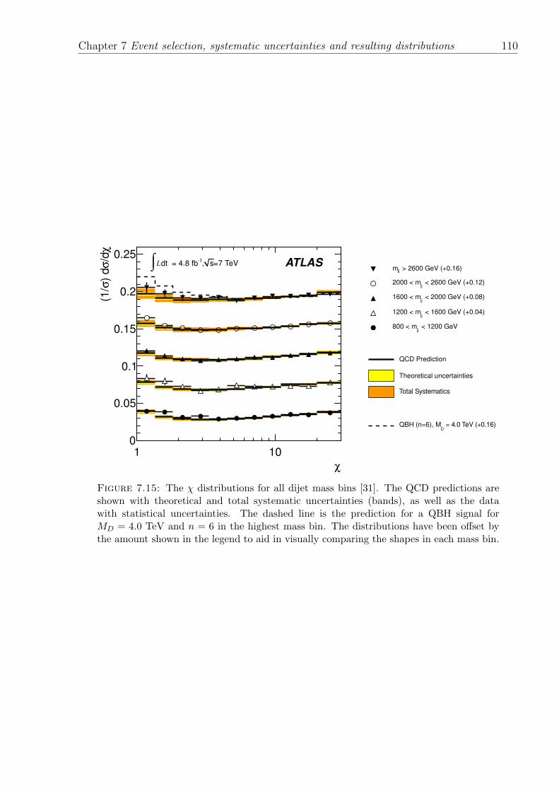
Chapter 7 Event selection, systematic uncertainties and resulting distributions 110
!1 10
!/d"
) d"(1
/
0
0.05
0.1
0.15
0.2
0.25=7 TeVs, -1dt = 4.8 fbL# ATLAS > 2600 GeV (+0.16)jjm
< 2600 GeV (+0.12)jj2000 < m
< 2000 GeV (+0.08)jj1600 < m
< 1600 GeV (+0.04)jj1200 < m
< 1200 GeVjj800 < m
QCD Prediction
Theoretical uncertainties
Total Systematics
= 4.0 TeV (+0.16)D
QBH (n=6), M
Figure 7.15: The χ distributions for all dijet mass bins [31]. The QCD predictions areshown with theoretical and total systematic uncertainties (bands), as well as the datawith statistical uncertainties. The dashed line is the prediction for a QBH signal forMD = 4.0 TeV and n = 6 in the highest mass bin. The distributions have been offset bythe amount shown in the legend to aid in visually comparing the shapes in each mass bin.
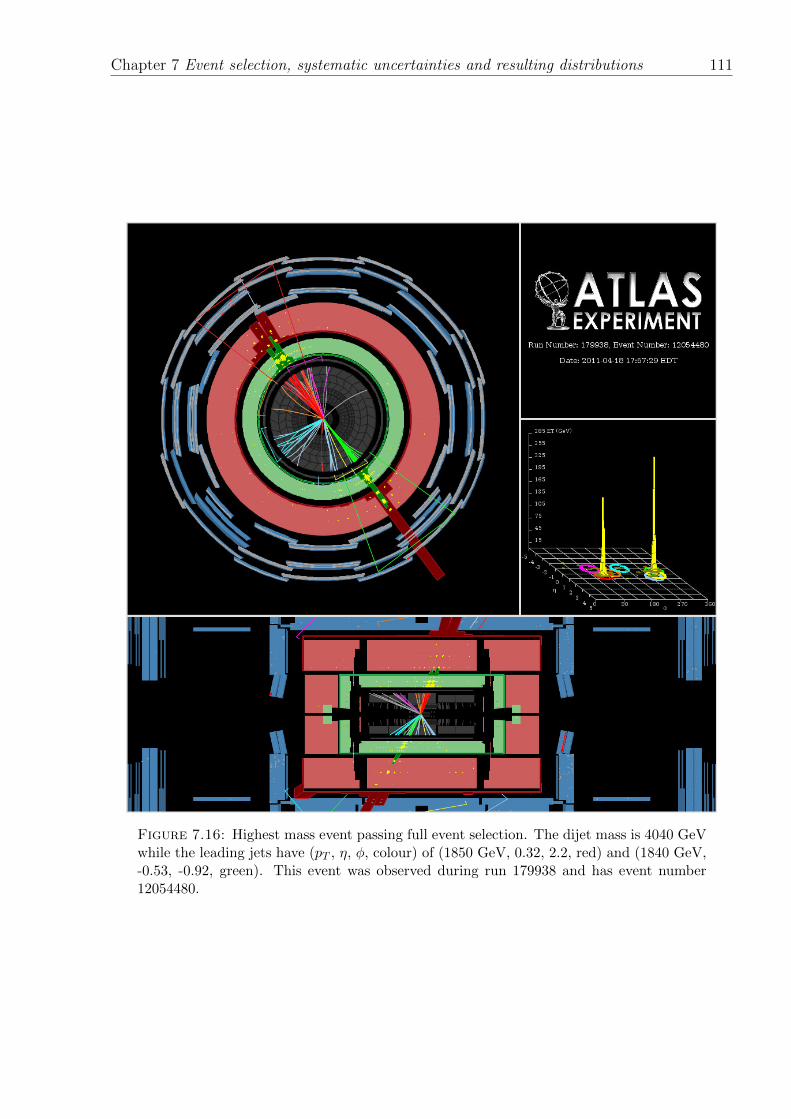
Chapter 7 Event selection, systematic uncertainties and resulting distributions 111
Figure 7.16: Highest mass event passing full event selection. The dijet mass is 4040 GeVwhile the leading jets have (pT , η, φ, colour) of (1850 GeV, 0.32, 2.2, red) and (1840 GeV,-0.53, -0.92, green). This event was observed during run 179938 and has event number12054480.
Chapter 8
Statistical interpretation and limits
on signals for new physics
When it comes to interpreting the results of the analysis, the strategy is clearly split between
a ‘search phase’ and a ‘limit-setting phase’.
The search phase is concerned with assessing to what extent the measured data agrees with
the simulated background prediction. Quantitatively, the most significant deviation of data
from the Monte Carlo (MC) is identified and a corresponding p−value that describes the
likelihood of such a deviation is calculated. In the event of reasonable agreement between
data and the MC prediction, we then proceed to the limit setting stage.
The purpose of the limit-setting phase is to assess the impact of the null-result from the
search phase on the phase space of New Physics (NP) scenarios. Multiple ‘benchmark’
models of NP processes are considered in this thesis, including: excited quarks, quark contact
interactions and Quantum Black Holes (see Chapter 4 for more details). One then asks the
question: if I assume that my NP model is valid, given the null-result in the search phase,
what constraints can I place on the free parameters of my model? Since the measurement
of data is subject to statistical and systematic uncertainties, it is only possible to constrain
model parameters at a certain Credibility Level (CL). Through constraint of NP model
parameters, these experimental results are able to guide theorists to reassess the plausibility
of many NP models and, where possible, provide direction for future work.
112
Chapter 8 Statistical interpretation and limits on signals for new physics 113
8.1 Search phase: is there evidence of new physics?
8.1.1 Hypothesis tests and calculation of p-values
In order to infer the presence of a new physical process, which is not currently included
in the SM, one must introduce a quantitative hypothesis test. A Null Hypothesis, H0, is
specified as that from which we search for a ‘significant’ deviation in data. The significance
required for the rejection of the null hypothesis must be specified as part of the procedure.
When testing the consistency of some data D with a null hypothesis H0, ‘pseudo-data’,
using Pseudo Experiments (PE), are produced that assumes H0. The p-value is calculated
in order to assess how the observed data compares to the N possible outcomes that H0 could
have produced:
p−value ≡ P(t ≥ t0|H0) (8.1)
where the test statistic1, t, is some function of the observable2. The test statistic is a random
variable, since it depends on how the pseudo-data fluctuate around H0. The observed test
statistic, t0, is the value of t corresponding to the value of the observable in data.
8.1.2 Bayes’ theorem
Bayes’ theorem gives the relationship between the probabilities of A and B, P(A) and P(B),
and the conditional probabilities of A given B and B given A, P(A|B) and P(B|A). For
proposition A and evidence B:
P(A|B) ∝ P(B|A) P(A), (8.2)
where P(A), the prior, is the initial degree of belief in A; P(B|A), the likelihood function,
is the probability of observing the evidence B assuming that the proposition A is true; and
P(A|B), the posterior, is the updated degree of belief in A having accounted for B. The
proportionality can be promoted to an equality by introducing a normalisation factor, which
will be denoted by N in the rest of this thesis.
1In this definition of p-value, it is assumed that a larger value of t corresponds to a larger differencebetween the data/pseud-data and H0.
2Considering an event A and an event B, the notation P(A|B) denotes the probability of event A occurring,given that event B occurred.
Chapter 8 Statistical interpretation and limits on signals for new physics 114
Consider N PE, of which S have t ≥ t0. The probability of observing S events with t ≥ t0
is given by the Binomial probability distribution3:
P(S|p−value) =
(N
S
)p−valueS(1− p−value)N−S. (8.3)
Using Bayes’ Theorem, the probability of obtaining a given p-value, given S out of N PE
having t ≥ t0, is:
P(p−value|S) =
(N
S
)p−valueS(1− p−value)N−S × π(p−value)
N (8.4)
where N is a normalisation constant and π(p−value) is the prior probability distribution.
For a uniform prior of π(p−value) = 1, the most likely result for the p-value4 is S/N . This
result allows us to determine a p-value using a finite number of pseudo-experiments.
The significance required for the rejection of H0 is defined as α, where we claim discovery
if p-value ≤ α, and α ∈ [0, 1]. Also, the probability to wrongly rule out H0 (known as a
“Type-I error”) is equal to α, namely5.
P (Type-I error) = P (p−value ≤ α|H0) = α. (8.5)
In general, a hypothesis test must be constructed using the following steps [145]:
• Define a test statistic, t, which describes the difference between data and H0. In this
thesis we shall use definitions of t for which a bigger difference between data and H0
corresponds to a larger value of t.
• Generate pseudo-experiments of H0 and find the distribution of the test statistic.
• Calculate a p-value of the test as the fraction of PE resulting in a test statistic greater
than, or equal to, the value observed in data.
Thus, the result of the test is a p-value. For a given α and a p-value = γ, if γ < α then
we would reject H0, and if γ > α then we would keep H0. For the first case (γ < α),
the discovery algorithm with the smallest Type-I error probability that would still declare
3The Binomial probability distribution function describes the probability of obtaining n successes, out ofN trials, given a probability of success p:
(Nn
)pn(1− p)N−n, where
(Nn
)= N !
n!(N−n)! .4This is found by solving ∂P(p−value|S)
∂(p−value) = 0.5It is shown in 8.1.5 that this is true no matter what hypothesis test the p-value is coming from, under
one condition: that there exist a solution ζ for which∫∞ζρt(x) dx = α, where ρt is the PDF followed by the
test statistic (t) under H0.
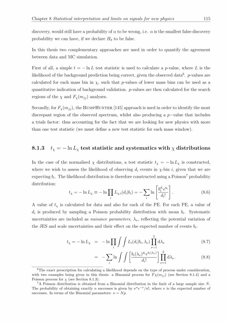
Chapter 8 Statistical interpretation and limits on signals for new physics 115
discovery, would still have a probability of α to be wrong, i.e. α is the smallest false-discovery
probability we can have, if we declare H0 to be false.
In this thesis two complementary approaches are used in order to quantify the agreement
between data and MC simulation.
First of all, a simple t = − lnL test statistic is used to calculate a p-value, where L is the
likelihood of the background prediction being correct, given the observed data6. p-values are
calculated for each mass bin in χ, such that p-values of lower mass bins can be used as a
quantitative indication of background validation. p-values are then calculated for the search
regions of the χ and Fχ(mjj) analyses.
Secondly, for Fχ(mjj), the BumpHunter [145] approach is used in order to identify the most
discrepant region of the observed spectrum, whilst also producing a p−value that includes
a trials factor: thus accounting for the fact that we are looking for new physics with more
than one test statistic (we must define a new test statistic for each mass window).
8.1.3 tχ = − lnLχ test statistic and systematics with χ distributions
In the case of the normalised χ distributions, a test statistic tχ = − lnLχ is constructed,
where we wish to assess the likelihood of observing di events in χ-bin i, given that we are
expecting bi. The likelihood distribution is therefore constructed using a Poisson7 probability
distribution:
tχ = − lnLχ ≡ − ln∏i
Lχ,i(di|bi) = −∑i
ln
[bdii e
bi
di!
]. (8.6)
A value of tχ is calculated for data and also for each of the PE. For each PE, a value of
di is produced by sampling a Poisson probability distribution with mean bi. Systematic
uncertainties are included as nuisance parameters, λν , reflecting the potential variation of
the JES and scale uncertainties and their effect on the expected number of events bi:
tχ = − lnLχ = − ln∏i
∫ ∫Li(di|bi, λν)
2∏ν=1
dλν (8.7)
= −∑i
ln
∫ ∫ [bi(λν)
diebi(λν)
di!
] 2∏ν=1
dλν . (8.8)
6The exact prescription for calculating a likelihood depends on the type of process under consideration,with two examples being given in this thesis: a Binomial process for Fχ(mjj) (see Section 8.1.4) and aPoisson process for χ (see Section 8.1.3).
7A Poisson distribution is obtained from a Binomial distribution in the limit of a large sample size N .The probability of obtaining exactly n successes is given by νne−ν/n!, where ν is the expected number ofsuccesses. In terms of the Binomial parameters: ν = Np.
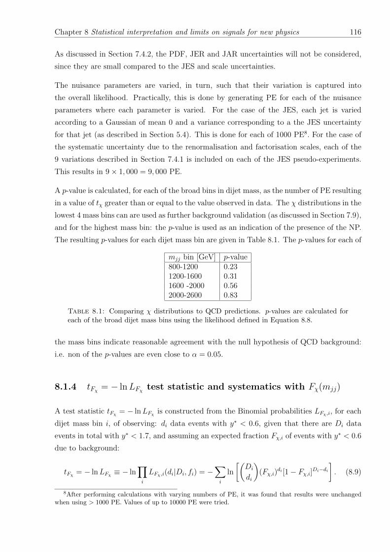
Chapter 8 Statistical interpretation and limits on signals for new physics 116
As discussed in Section 7.4.2, the PDF, JER and JAR uncertainties will not be considered,
since they are small compared to the JES and scale uncertainties.
The nuisance parameters are varied, in turn, such that their variation is captured into
the overall likelihood. Practically, this is done by generating PE for each of the nuisance
parameters where each parameter is varied. For the case of the JES, each jet is varied
according to a Gaussian of mean 0 and a variance corresponding to a the JES uncertainty
for that jet (as described in Section 5.4). This is done for each of 1000 PE8. For the case of
the systematic uncertainty due to the renormalisation and factorisation scales, each of the
9 variations described in Section 7.4.1 is included on each of the JES pseudo-experiments.
This results in 9× 1, 000 = 9, 000 PE.
A p-value is calculated, for each of the broad bins in dijet mass, as the number of PE resulting
in a value of tχ greater than or equal to the value observed in data. The χ distributions in the
lowest 4 mass bins can are used as further background validation (as discussed in Section 7.9),
and for the highest mass bin: the p-value is used as an indication of the presence of the NP.
The resulting p-values for each dijet mass bin are given in Table 8.1. The p-values for each of
mjj bin [GeV] p-value800-1200 0.231200-1600 0.311600 -2000 0.562000-2600 0.83
Table 8.1: Comparing χ distributions to QCD predictions. p-values are calculated foreach of the broad dijet mass bins using the likelihood defined in Equation 8.8.
the mass bins indicate reasonable agreement with the null hypothesis of QCD background:
i.e. non of the p-values are even close to α = 0.05.
8.1.4 tFχ = − lnLFχ test statistic and systematics with Fχ(mjj)
A test statistic tFχ = − lnLFχ is constructed from the Binomial probabilities LFχ,i, for each
dijet mass bin i, of observing: di data events with y∗ < 0.6, given that there are Di data
events in total with y∗ < 1.7, and assuming an expected fraction Fχ,i of events with y∗ < 0.6
due to background:
tFχ = − lnLFχ ≡ − ln∏i
LFχ,i(di|Di, fi) = −∑i
ln
[(Di
di
)(Fχ,i)
di [1− Fχ,i]Di−di]. (8.9)
8After performing calculations with varying numbers of PE, it was found that results were unchangedwhen using > 1000 PE. Values of up to 10000 PE were tried.
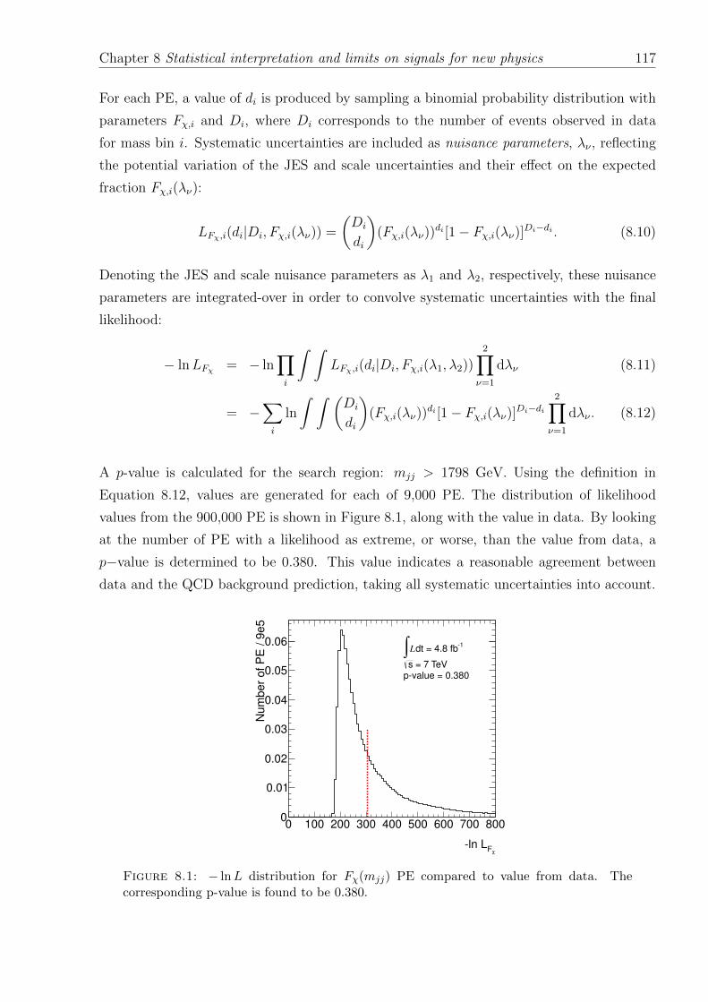
Chapter 8 Statistical interpretation and limits on signals for new physics 117
For each PE, a value of di is produced by sampling a binomial probability distribution with
parameters Fχ,i and Di, where Di corresponds to the number of events observed in data
for mass bin i. Systematic uncertainties are included as nuisance parameters, λν , reflecting
the potential variation of the JES and scale uncertainties and their effect on the expected
fraction Fχ,i(λν):
LFχ,i(di|Di, Fχ,i(λν)) =
(Di
di
)(Fχ,i(λν))
di [1− Fχ,i(λν)]Di−di . (8.10)
Denoting the JES and scale nuisance parameters as λ1 and λ2, respectively, these nuisance
parameters are integrated-over in order to convolve systematic uncertainties with the final
likelihood:
− lnLFχ = − ln∏i
∫ ∫LFχ,i(di|Di, Fχ,i(λ1, λ2))
2∏ν=1
dλν (8.11)
= −∑i
ln
∫ ∫ (Di
di
)(Fχ,i(λν))
di [1− Fχ,i(λν)]Di−di2∏
ν=1
dλν . (8.12)
A p-value is calculated for the search region: mjj > 1798 GeV. Using the definition in
Equation 8.12, values are generated for each of 9,000 PE. The distribution of likelihood
values from the 900,000 PE is shown in Figure 8.1, along with the value in data. By looking
at the number of PE with a likelihood as extreme, or worse, than the value from data, a
p−value is determined to be 0.380. This value indicates a reasonable agreement between
data and the QCD background prediction, taking all systematic uncertainties into account.
χFln L
0 100 200 300 400 500 600 700 800
Num
ber
of P
E / 9
e5
0
0.01
0.02
0.03
0.04
0.05
0.06 1dt = 4.8 fbL∫ = 7 TeVs
pvalue = 0.380
Figure 8.1: − lnL distribution for Fχ(mjj) PE compared to value from data. Thecorresponding p-value is found to be 0.380.
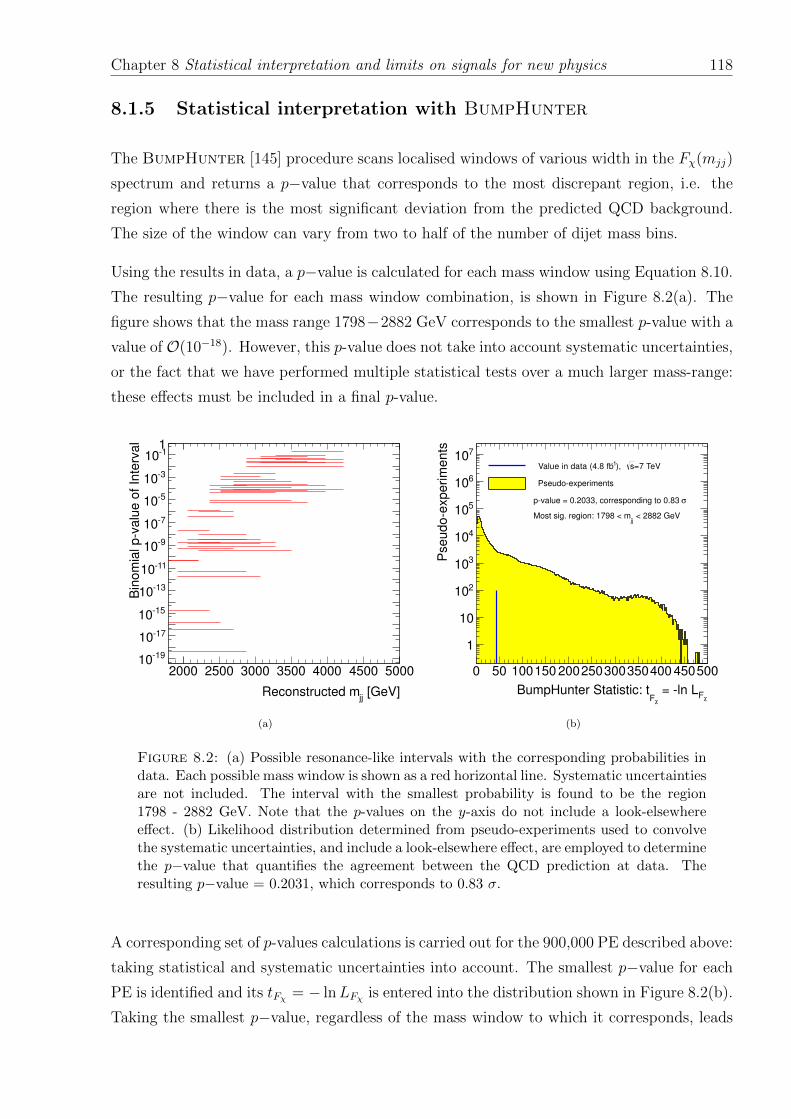
Chapter 8 Statistical interpretation and limits on signals for new physics 118
8.1.5 Statistical interpretation with BumpHunter
The BumpHunter [145] procedure scans localised windows of various width in the Fχ(mjj)
spectrum and returns a p−value that corresponds to the most discrepant region, i.e. the
region where there is the most significant deviation from the predicted QCD background.
The size of the window can vary from two to half of the number of dijet mass bins.
Using the results in data, a p−value is calculated for each mass window using Equation 8.10.
The resulting p−value for each mass window combination, is shown in Figure 8.2(a). The
figure shows that the mass range 1798−2882 GeV corresponds to the smallest p-value with a
value of O(10−18). However, this p-value does not take into account systematic uncertainties,
or the fact that we have performed multiple statistical tests over a much larger mass-range:
these effects must be included in a final p-value.
[GeV]jj
Reconstructed m
2000 2500 3000 3500 4000 4500 5000
Bin
om
ial pv
alu
e o
f In
terv
al
1910
1710
1510
1310
1110
910
710
510
310
1101
(a)
χF = ln LχF
BumpHunter Statistic: t
0 50 100150 200250300350400 450500
Pseudoe
xperim
ents
1
10
210
310
410
510
610
710=7 TeVs), 1 Value in data (4.8 fb
Pseudoexperiments
σpvalue = 0.2033, corresponding to 0.83
< 2882 GeVjj
Most sig. region: 1798 < m
(b)
Figure 8.2: (a) Possible resonance-like intervals with the corresponding probabilities indata. Each possible mass window is shown as a red horizontal line. Systematic uncertaintiesare not included. The interval with the smallest probability is found to be the region1798 - 2882 GeV. Note that the p-values on the y-axis do not include a look-elsewhereeffect. (b) Likelihood distribution determined from pseudo-experiments used to convolvethe systematic uncertainties, and include a look-elsewhere effect, are employed to determinethe p−value that quantifies the agreement between the QCD prediction at data. Theresulting p−value = 0.2031, which corresponds to 0.83 σ.
A corresponding set of p-values calculations is carried out for the 900,000 PE described above:
taking statistical and systematic uncertainties into account. The smallest p−value for each
PE is identified and its tFχ = − lnLFχ is entered into the distribution shown in Figure 8.2(b).
Taking the smallest p−value, regardless of the mass window to which it corresponds, leads

Chapter 8 Statistical interpretation and limits on signals for new physics 119
to the inclusion of a trials factor: allowing for the fact that there is no prior belief for a
discrepancy to appear at any particular mass range.
Comparing the value of tFχ in data to the distribution in Figure 8.2(b), we calculate a p-
value of 0.2031, which corresponds to a 0.83 σ deviation from the null hypothesis. This result
provides no evidence for a significant deviation from our null hypothesis, and therefore no
evidence for NP.
8.1.5.1 TailHunter configuration
An alternative configuration of the BumpHunter, known as the TailHunter, is used to
search for slow onset effects at the high-mass end of the distribution. The upper edge of
each mass window is fixed to the highest dijet mass bin in the spectrum and the search
window is then expanded downward, to include lower bins. The method then proceeds in
the same vein as the BumpHunter and the results are shown in Figures 8.3(a) and 8.3(b).
The most discrepant region in data corresponds to the region mjj > 1798 GeV (i.e. the
[GeV]jj
Reconstructed m
2000 2500 3000 3500 4000 4500 5000
Bin
om
ial pv
alu
e o
f In
terv
al
2110
1910
1710
1510
1310
1110
910
710
510
310
1101
(a)
χF = ln LχF
TailHunter Statistic: t
0 50 100150 200250300350400 450500
Pseudoe
xperim
ents
1
10
210
310
410
510
610
710=7 TeVs), 1 Value in data (4.8 fb
Pseudoexperiments
σpvalue = 0.2110, corresponding to 0.80
> 1798 GeVjj
Most sig. region: m
(b)
Figure 8.3: (a) Possible threshold-like intervals with the corresponding probabilities indata. Each possible mass window is shown as a red horizontal line. Systematic uncertaintiesare not included. The interval with the smallest probability is found to be the regionmjj > 1798 GeV. Note that the p-values on the y-axis do not include a look-elsewhereeffect. (b) Likelihood distribution determined from pseudo-experiments used to convolvethe systematic uncertainties are employed to determine the p−value that quantifies theagreement between the QCD prediction at data. The resulting p−value = 0.2111, whichcorresponds to 0.80 σ.

Chapter 8 Statistical interpretation and limits on signals for new physics 120
whole mass range), with a p-value = 0.2111, corresponding to a 0.80 σ deviation from the
null hypothesis. Again, this result indicates no evidence for NP.
Chapter 8 Statistical interpretation and limits on signals for new physics 121
8.2 Limit-setting phase: constraints on new physics
In order to draw quantitative conclusions from a search for new physics, a null hypothesis
and at least one alternative hypothesis is defined. In this thesis, alternative hypotheses
consist of particular new physics models, for which a model parameter is allowed to vary.
In this case, an upper or lower limit can be placed on the values of this free parameter, at
some credibility level. For example, in a BSM scenario with extra dimensions it is useful
to establish which values of the fundamental Planck mass have been excluded by the data.
Since data are subject to statistical fluctuations, one must define a convention from which a
conclusion can be drawn that is beyond reasonable doubt. In this thesis, limits are set at the
(1− α) = 95% credibility level.
8.2.1 Acceptance for signal samples
In Figure 8.4, the acceptance × efficiency for each signal considered in this thesis. These
values are calculated by comparing the initial number of events in each MC sample, to the
the number of events passing the complete event selection specified in Section 7.1. Values
are shown as a function of the signal model parameters: i.e. MD for the QBH samples, Mq∗
for the excited quarks and Λ for the contract interactions.
It can be seen that the acceptance and efficiency are roughly constant across the respective
parameter ranges. In the remainder of this thesis, the combined acceptance × efficiency is
denoted by A.
8.2.2 Limit setting with Fχ(mjj)
As discussed in previous chapters, the Fχ(mjj) spectrum is sensitive to both resonant NP
and also processes with a slow-onset in mass. Example distributions of the signal samples
considered in this thesis are shown in Figure 6.9.
Two different limit setting approaches are employed depending on whether the signal model
under consideration interferes with the QCD background. For models such as excited quarks
and quantum black holes, which do not interfere with QCD, there is the possibility to
calculate a limit on the cross-section times acceptance for the model across the whole mass
spectrum. An alternative method must be used in the case of quark contact interactions.
The distinction between the two cases is made clear in the following two subsections.
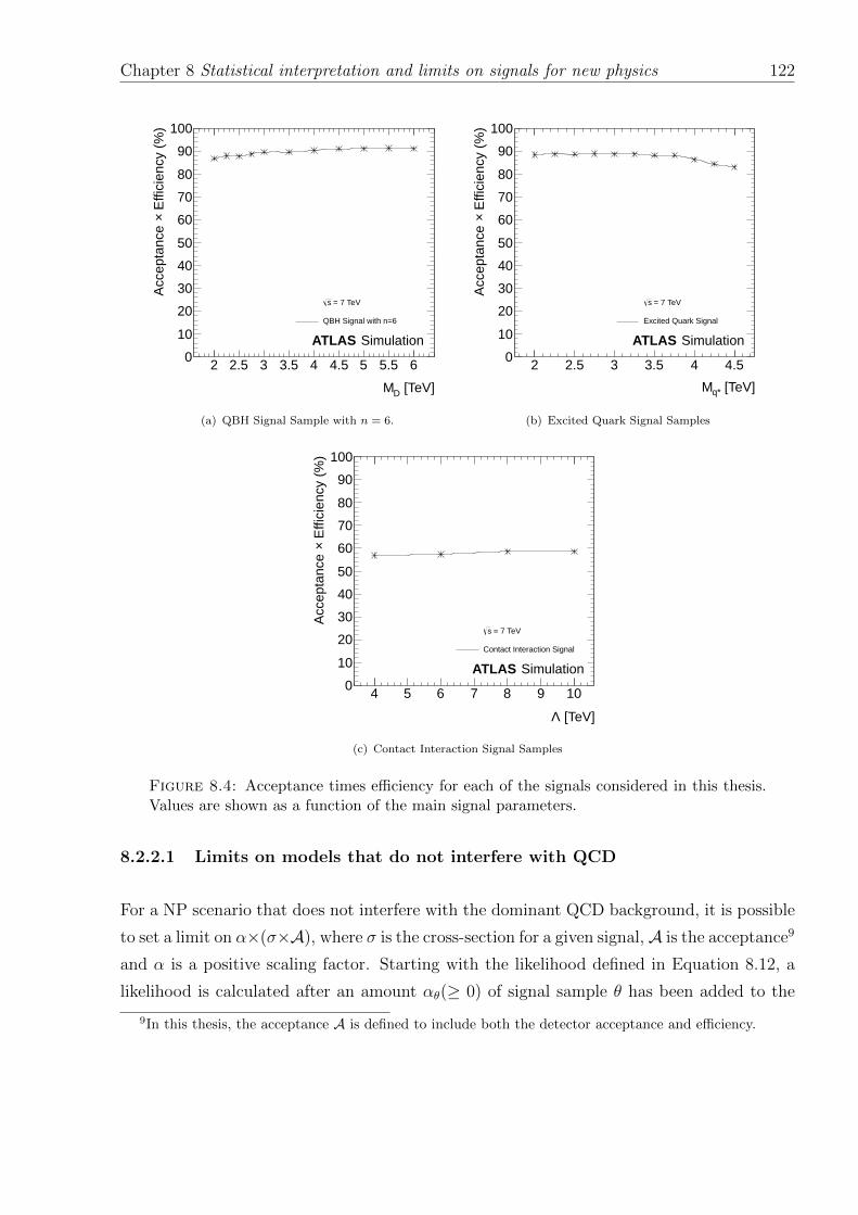
Chapter 8 Statistical interpretation and limits on signals for new physics 122
[TeV]DM
2 2.5 3 3.5 4 4.5 5 5.5 6
Effi
cien
cy (
%)
×A
ccep
tanc
e
0
10
20
30
40
50
60
70
80
90
100
= 7 TeVs
QBH Signal with n=6
ATLAS Simulation
(a) QBH Signal Sample with n = 6.
[TeV]q*M
2 2.5 3 3.5 4 4.5
Effi
cien
cy (
%)
×A
ccep
tanc
e
0
10
20
30
40
50
60
70
80
90
100
= 7 TeVs
Excited Quark Signal
ATLAS Simulation
(b) Excited Quark Signal Samples
[TeV]Λ
4 5 6 7 8 9 10
Effi
cien
cy (
%)
×A
ccep
tanc
e
0
10
20
30
40
50
60
70
80
90
100
= 7 TeVs
Contact Interaction Signal
ATLAS Simulation
(c) Contact Interaction Signal Samples
Figure 8.4: Acceptance times efficiency for each of the signals considered in this thesis.Values are shown as a function of the main signal parameters.
8.2.2.1 Limits on models that do not interfere with QCD
For a NP scenario that does not interfere with the dominant QCD background, it is possible
to set a limit on α×(σ×A), where σ is the cross-section for a given signal, A is the acceptance9
and α is a positive scaling factor. Starting with the likelihood defined in Equation 8.12, a
likelihood is calculated after an amount αθ(≥ 0) of signal sample θ has been added to the
9In this thesis, the acceptance A is defined to include both the detector acceptance and efficiency.
Chapter 8 Statistical interpretation and limits on signals for new physics 123
NLO QCD background10:
LFχ,i(di|Di, Fχ,i(λν))→ LFχ,i(di|Di, Fχ,i(αθ, λν)),
where Fχ,i is now a function of αθ, as well as a function of each λν . In a given mass bin, the
number of QCD background events with |y∗| < 0.6 and |y∗| < 1.7 are denoted by binner and
btotal, respectively. The corresponding number of events from the signal prediction are αsinner
and αstotal. The expected value of Fχ,i(α) is therefore given by (binner + αsinner)/(btotal +
αstotal). Since the signal prediction is also subject to nuisance parameters:
Fχ,i(α, λν) =binner(λν) + αsinner(λν)
btotal(λν) + αstotal(λν). (8.13)
Using Bayes Theorem (See Equation 8.4), a limit can then calculated at the 95% CL:
0.95 =
∫ αlimitθ
0
LFχ(Fχ(αθ)|di, Di) dαθ (8.14)
=
∫ αlimiθ
0
LFχ(di|Fχ(αθ), Di)×π(Fχ(αθ, Di))
N dαθ (8.15)
=1
N
∫ αlimitθ
0
∑i
ln
∫ ∫ [(Di
di
)Fχ,i(αθ, λν)
di [1− Fχ,i(αθ, λν)]Di−di] 2∏ν=1
dλνdαθ,
where a constant prior, π(Fχ, Di) has been assumed11.
In practice, values of αθ are chosen according to12:
αθ(n) = 10(−5+10n/1000), (8.16)
where n = 1, . . . , 1000. These choices of αθ ensure a full coverage over the full range of 10−5
to 105. Increasing the number of steps was found to have an insignificant effect on the final
result, and a range of 10−5 to 105 in αθ was found to be sufficient to contain the limit of
each signal.
For each value of αθ, the likelihood is calculated, as described in the previous section. A
sum is formed of the likelihoods of increasing values of αθ (normalised to the total sum of all
likelihoods) to a value of 0.95. The value of αθ corresponding to last likelihood in the sum,
10As described in Chapter 7, the NLO QCD background is produced by multiplying LO QCD spectra forFχ(mjj) and χ with bin-wise NLO k-factors.
11This is a reasonable assumption, since there is no reason to prefer one version of new physics to another.12Note that the final limit figures (e.g. Figure 8.5) are plotted with a log-scale on the y-axis. The
distribution of αθ is chosen to reflect the distribution of the resulting likelihoods and ensure a good coverageover the full range of αθ.
Chapter 8 Statistical interpretation and limits on signals for new physics 124
is αlimitθ :
0.95 =
∑αθ=αlimitθ
αθ=10−5 LFχ(di|Fχ(αθ), Di)∑αθ=105
αθ=10−5 LFχ(di|Fχ(αθ), Di). (8.17)
For each signal sample, θ, a value of αlimitθ is calculated in data and for each PE. Looking at
Figure 8.5, as an example of a limit setting procedure for an excited quark, the black points
represent the values of αlimitθ × σθ × A, from data, for each of the signal samples (which
are parameterised by different excited quark masses). The black dashed line surrounded by
green and yellow bands represent the mean, 1-σ and 2-σ values in the distribution of αlimitθ
values coming from the 900,000 PEs.
The red dotted line in the figure, is formed from the values of σθ×A for each signal sample.
The points where the black dashed curve and the black solid curve cross the red dotted curve
determine the expected and observed upper limits on the model parameter13, respectively.
Limits are set on both the excited quark model (q∗) and the quantum black hole model
(QBH). The resulting limits for the excited quark (with the corrected FSR as explained in
Section 4.3) are shown in Figure 8.5. The analysis results in a lower limit on the mass of
the q∗, with an expected limit of 2.85 TeV and an observed limit of 2.75 TeV. Acceptance
values for the q∗ mass points range between 86-89%.
For the Pythia 6 excited quark model with the mis-calculated FSR, the observed (expected)
limit is 2.86 TeV (2.95 TeV). This result in included in order to aid comparison to previous
ATLAS limits, as well as limits set by other experiments.
In the case of the QBH model, the limit setting is performed using signal samples with
n = 6 extra dimensions. Truth level distributions for QBH samples with a range of values
of n are shown in Figure 8.6. Figure 8.6(a) shows the normalised χ distributions for values
of n ranging from 3 to 7 - note that these distributions do not include QCD. Since these
distributions are normalised (and given they do not contain any SM QCD background) it is
clear that the angular distribution is independent of n. Figure 8.6(b) shows the cumulative
distributions of the normalised cross-section for values of n ranging from 3 to 7 - again, note
that these distributions do not include QCD. The fact that the cumulative dijet mass profile
for QBH is largely independent of n above the dijet mass thresholds that we are considering,
also suggests an acceptance independent of n in this mass region.
It is clear that the mass profile for the QBH samples is also largely independent of n. It is
therefore concluded that the acceptance of a given QBH signal mass point, is independent of
13In the case of Figure 8.5, the model parameter, on which limits are set, is the mass of the excited quark:mq∗ .

Chapter 8 Statistical interpretation and limits on signals for new physics 125
Mass [GeV]2000 2500 3000 3500 4000 4500
[pb]
× m
-310
-210
-110
1
10
210
310
ATLAS
q* Observed 95% CL upper limit Expected 95% CL upper limit 68% band 95% band
=7 TeVs, -1dt = 4.8 fbL0
Figure 8.5: The 95% CL upper limits of σ × A as a function of the q∗ mass usingFχ(mjj) (black filled circles). The black dashed curve shows the 95% CL upper limitexpected from Monte Carlo and the light and dark yellow shaded bands represent the 68%and 95% contours of the expected limit, respectively. Theoretical predictions of σ ×A forthe excited quark model as shown as dotted lines. The observed (expected) limit occurs atthe crossing of the theory curve with the observed (expected) 95% CL upper limit curve.
n extra Expected Observeddimensions limit (TeV) limit (TeV)
2 3.85 3.713 3.99 3.844 4.07 3.925 4.12 3.996 4.16 4.037 4.19 4.07
Table 8.2: Lower limits at the 95% CL on MD of the QBH model with n = 2− 7 extradimensions.
the number of extra spatial dimensions. The acceptance of the fully-simulated n = 6 QBH
sample, which is close to 90 % for all values of MD, is then used as the acceptance for other
values of n and the resulting theory lines can be included in Figure 8.7. The resulting limits
on the reduced Planck Scale MD for the QBH model are shown in Table 8.2.
This approach to limit setting is dependent upon the ability to add an arbitrary amount of
signal to the QCD background, which can only easily be done for models where interference
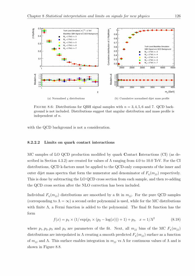
Chapter 8 Statistical interpretation and limits on signals for new physics 126
1 10
χ(1
/N)d
N/d
0
0.1
0.2
0.3
0.4
0.5 > 2 TeV
truth
jjTruth Level Simulation, m
BlackMax QBH Signal w/o QCD Background
= 2 TeV, n = 3D
M
= 2 TeV, n = 4D
M
= 2 TeV, n = 5D
M
= 2 TeV, n = 6D
M
= 2 TeV, n = 7D
M
χ
1 10
Mo
de
l/n
=6
0.40.60.8
11.21.41.6
(a) Normalised χ distributions
2000 2500 3000 3500 4000 4500
jjC
um
ula
tive
dis
trib
utio
n o
f (1
/N)d
N/d
m
0.2
0.3
0.4
0.5
0.6
0.7
0.8
0.9
1
Truth Level BlackMax Simulation
QBH Signal w/o QCD Background
= 2 TeV, n = 3D
M
= 2 TeV, n = 4D
M
= 2 TeV, n = 5D
M
= 2 TeV, n = 6D
M
= 2 TeV, n = 7D
M
[GeV]jjm
2000 2500 3000 3500 4000 4500
Mo
de
l/n
=6
00.20.40.60.8
11.21.41.61.8
2
(b) Cumulative normalised dijet mass profile
Figure 8.6: Distributions for QBH signal samples with n = 3, 4, 5, 6 and 7. QCD back-ground is not included. Distributions suggest that angular distribution and mass profile isindependent of n.
with the QCD background is not a consideration.
8.2.2.2 Limits on quark contact interactions
MC samples of LO QCD production modified by quark Contact Interactions (CI) (as de-
scribed in Section 4.3.2) are created for values of Λ ranging from 4.0 to 10.0 TeV. For the CI
distributions, QCD k-factors must be applied to the QCD-only components of the inner and
outer dijet mass spectra that form the numerator and denominator of Fχ(mjj) respectively.
This is done by subtracting the LO QCD cross section from each sample, and then re-adding
the QCD cross section after the NLO correction has been included.
Individual Fχ(mjj) distributions are smoothed by a fit in mjj. For the pure QCD samples
(corresponding to Λ =∞) a second order polynomial is used, while for the MC distributions
with finite Λ, a Fermi function is added to the polynomial. The final fit function has the
form
f(x) = p4 × (1/ exp(p1 × (p2 − log(x))) + 1) + p3, x = 1/Λ2 (8.18)
where p1, p2, p3 and p4 are parameters of the fit. Next, all mjj bins of the MC Fχ(mjj)
distributions are interpolated in Λ creating a smooth predicted Fχ(mjj) surface as a function
of mjj and Λ. This surface enables integration in mjj vs Λ for continuous values of Λ and is
shown in Figure 8.8.
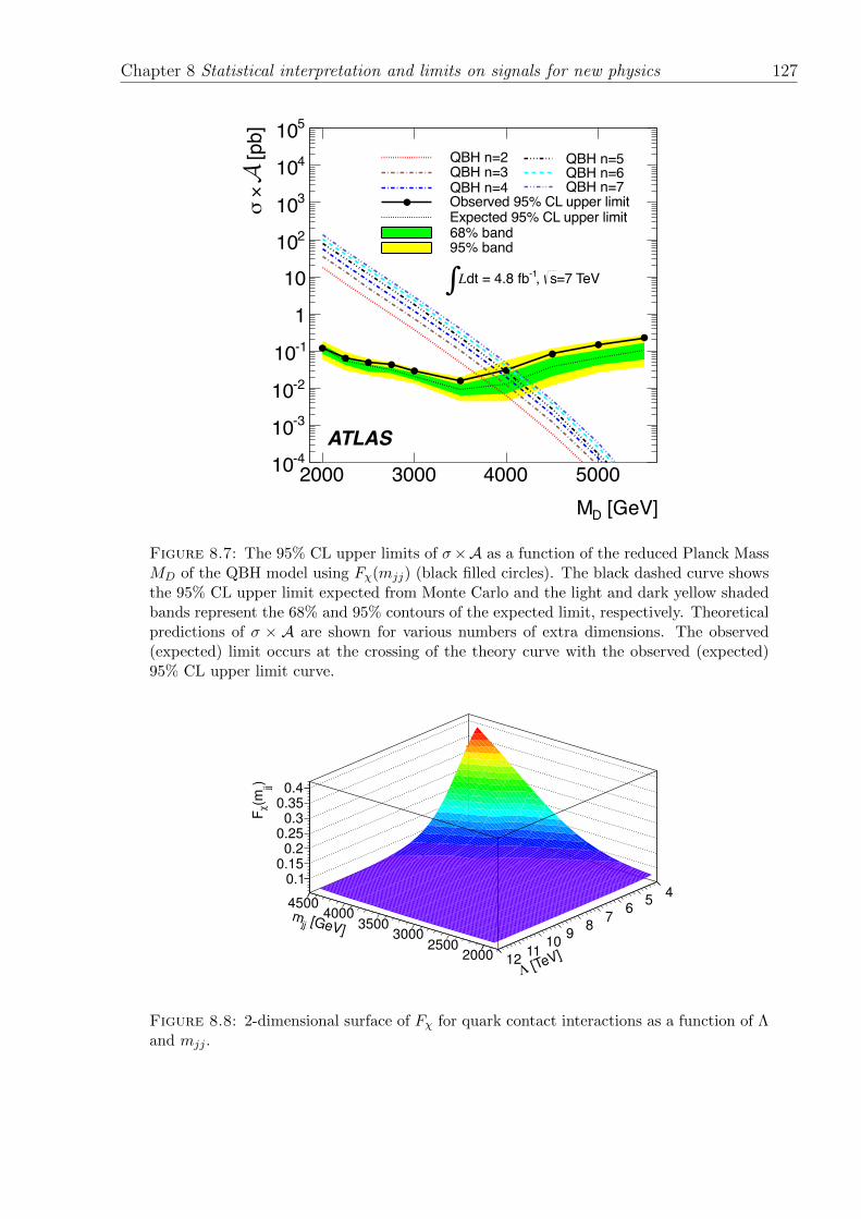
Chapter 8 Statistical interpretation and limits on signals for new physics 127
[GeV]DM2000 3000 4000 5000
[pb]
× m
-410
-310
-210
-110
1
10
210
310
410
510
ATLAS
QBH n=2 QBH n=3 QBH n=4 Observed 95% CL upper limit Expected 95% CL upper limit 68% band 95% band
QBH n=5 QBH n=6 QBH n=7
=7 TeVs, -1dt = 4.8 fbL0
Figure 8.7: The 95% CL upper limits of σ×A as a function of the reduced Planck MassMD of the QBH model using Fχ(mjj) (black filled circles). The black dashed curve showsthe 95% CL upper limit expected from Monte Carlo and the light and dark yellow shadedbands represent the 68% and 95% contours of the expected limit, respectively. Theoreticalpredictions of σ × A are shown for various numbers of extra dimensions. The observed(expected) limit occurs at the crossing of the theory curve with the observed (expected)95% CL upper limit curve.
[GeV]jjm
20002500
30003500
40004500
[TeV]Λ
45
67
89
1011
12
) jj(m
χF
0.10.150.2
0.250.3
0.350.4
Figure 8.8: 2-dimensional surface of Fχ for quark contact interactions as a function of Λand mjj .
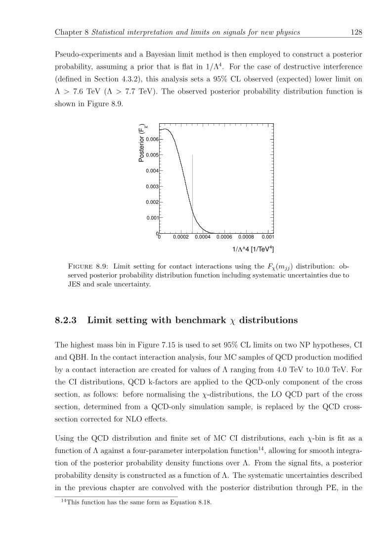
Chapter 8 Statistical interpretation and limits on signals for new physics 128
Pseudo-experiments and a Bayesian limit method is then employed to construct a posterior
probability, assuming a prior that is flat in 1/Λ4. For the case of destructive interference
(defined in Section 4.3.2), this analysis sets a 95% CL observed (expected) lower limit on
Λ > 7.6 TeV (Λ > 7.7 TeV). The observed posterior probability distribution function is
shown in Figure 8.9.
]4^4 [1/TeVΛ1/
0 0.0002 0.0004 0.0006 0.0008 0.001
)χ
Po
ste
rio
r (F
0
0.001
0.002
0.003
0.004
0.005
0.006
Figure 8.9: Limit setting for contact interactions using the Fχ(mjj) distribution: ob-served posterior probability distribution function including systematic uncertainties due toJES and scale uncertainty.
8.2.3 Limit setting with benchmark χ distributions
The highest mass bin in Figure 7.15 is used to set 95% CL limits on two NP hypotheses, CI
and QBH. In the contact interaction analysis, four MC samples of QCD production modified
by a contact interaction are created for values of Λ ranging from 4.0 TeV to 10.0 TeV. For
the CI distributions, QCD k-factors are applied to the QCD-only component of the cross
section, as follows: before normalising the χ-distributions, the LO QCD part of the cross
section, determined from a QCD-only simulation sample, is replaced by the QCD cross-
section corrected for NLO effects.
Using the QCD distribution and finite set of MC CI distributions, each χ-bin is fit as a
function of Λ against a four-parameter interpolation function14, allowing for smooth integra-
tion of the posterior probability density functions over Λ. From the signal fits, a posterior
probability density is constructed as a function of Λ. The systematic uncertainties described
in the previous chapter are convolved with the posterior distribution through PE, in the
14This function has the same form as Equation 8.18.
Chapter 8 Statistical interpretation and limits on signals for new physics 129
same way as the Fχ(mjj) analysis. For the expected limit, PE are performed on the QCD
background and used as pseudo-data: as with the Fχ(mjj) analysis. This analysis sets a
95% CL lower limit on Λ at 7.6 TeV with an expected limit of 7.7 TeV.
An analogous method is used to set limits on QBH, using eleven signal samples with MD
ranging from 2.0 TeV to 6.0 TeV. A constant prior in 1/M4D is used, since this is proportional
to the cross-section. This analysis results in an expected and observed 95% CL lower limit
on MD of 4.20 TeV and 4.11 TeV, respectively.
Chapter 9
Summary and conclusions
9.1 Summary of results
In this chapter, the results of this thesis will be summarised, and compared to results form
independent analysis methods and experiments. Possible future analyses and developments
are also discussed, before concluding.
9.1.1 Results from search phase
Angular distributions of jet pairs (dijets) produced in proton-proton collisions at a centre-of-
mass energy√s = 7 TeV have been studied with the ATLAS detector at the Large Hadron
Collider using the full 2011 data set with an integrated luminosity of 4.8 fb−1, and reaching
dijet masses up to 4.5 TeV.
Searches are made by comparing data to an NLO QCD MC simulation, which presents the
dominant background for a search of this kind. The associated systematic uncertainties
have been considered, with the dominant contributions being due to the Jet Energy Scale
uncertainty and the uncertainty on the renormalisation and factorisation scale, µR and µF .
Searches have been performed by slicing the dijet angular-mass phase space in two ways:
normalised χ distributions are more sensitive to angular information, with a course bins of
dijet mass; whilst Fχ(mjj) sacrifices some angular information in order to take advantage of
a finer granularity in mass.
130
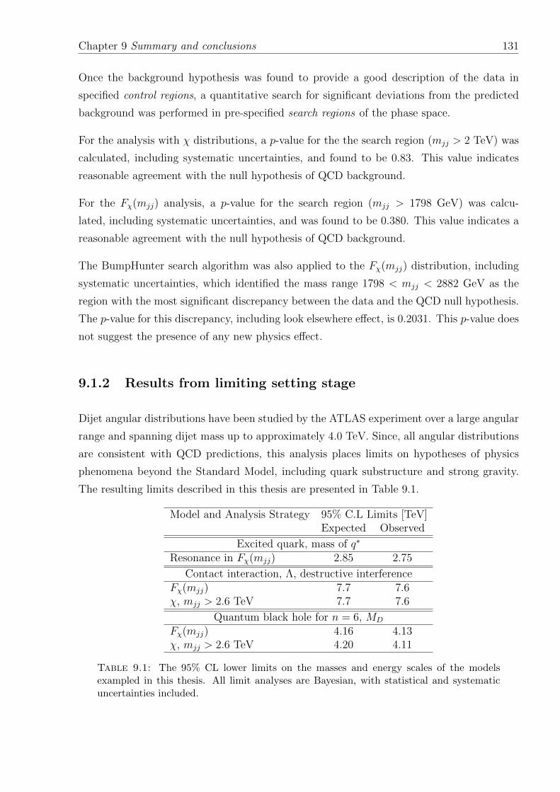
Chapter 9 Summary and conclusions 131
Once the background hypothesis was found to provide a good description of the data in
specified control regions, a quantitative search for significant deviations from the predicted
background was performed in pre-specified search regions of the phase space.
For the analysis with χ distributions, a p-value for the the search region (mjj > 2 TeV) was
calculated, including systematic uncertainties, and found to be 0.83. This value indicates
reasonable agreement with the null hypothesis of QCD background.
For the Fχ(mjj) analysis, a p-value for the search region (mjj > 1798 GeV) was calcu-
lated, including systematic uncertainties, and was found to be 0.380. This value indicates a
reasonable agreement with the null hypothesis of QCD background.
The BumpHunter search algorithm was also applied to the Fχ(mjj) distribution, including
systematic uncertainties, which identified the mass range 1798 < mjj < 2882 GeV as the
region with the most significant discrepancy between the data and the QCD null hypothesis.
The p-value for this discrepancy, including look elsewhere effect, is 0.2031. This p-value does
not suggest the presence of any new physics effect.
9.1.2 Results from limiting setting stage
Dijet angular distributions have been studied by the ATLAS experiment over a large angular
range and spanning dijet mass up to approximately 4.0 TeV. Since, all angular distributions
are consistent with QCD predictions, this analysis places limits on hypotheses of physics
phenomena beyond the Standard Model, including quark substructure and strong gravity.
The resulting limits described in this thesis are presented in Table 9.1.
Model and Analysis Strategy 95% C.L Limits [TeV]Expected Observed
Excited quark, mass of q∗
Resonance in Fχ(mjj) 2.85 2.75
Contact interaction, Λ, destructive interferenceFχ(mjj) 7.7 7.6χ, mjj > 2.6 TeV 7.7 7.6
Quantum black hole for n = 6, MD
Fχ(mjj) 4.16 4.13χ, mjj > 2.6 TeV 4.20 4.11
Table 9.1: The 95% CL lower limits on the masses and energy scales of the modelsexampled in this thesis. All limit analyses are Bayesian, with statistical and systematicuncertainties included.
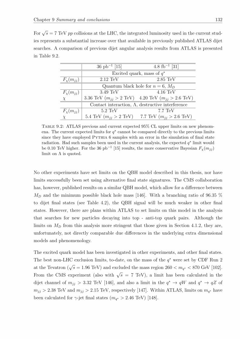
Chapter 9 Summary and conclusions 132
For√s = 7 TeV pp collisions at the LHC, the integrated luminosity used in the current stud-
ies represents a substantial increase over that available in previously published ATLAS dijet
searches. A comparison of previous dijet angular analysis results from ATLAS is presented
in Table 9.2.
36 pb−1 [15] 4.8 fb−1 [31]
Excited quark, mass of q∗
Fχ(mjj) 2.12 TeV 2.85 TeV
Quantum black hole for n = 6, MD
Fχ(mjj) 3.49 TeV 4.16 TeVχ 3.36 TeV (mjj > 2 TeV) 4.20 TeV (mjj > 2.6 TeV)
Contact interaction, Λ, destructive interferenceFχ(mjj) 5.2 TeV 7.7 TeVχ 5.4 TeV (mjj > 2 TeV) 7.7 TeV (mjj > 2.6 TeV)
Table 9.2: ATLAS previous and current expected 95% CL upper limits on new phenom-ena. The current expected limits for q∗ cannot be compared directly to the previous limitssince they have employed Pythia 6 samples with an error in the simulation of final stateradiation. Had such samples been used in the current analysis, the expected q∗ limit wouldbe 0.10 TeV higher. For the 36 pb−1 [15] results, the more conservative Bayesian Fχ(mjj)limit on Λ is quoted.
No other experiments have set limits on the QBH model described in this thesis, nor have
limits successfully been set using alternative final state signatures. The CMS collaboration
has, however, published results on a similar QBH model, which allow for a difference between
MD and the minimum possible black hole mass [146]. With a branching ratio of 96.35 %
to dijet final states (see Table 4.2), the QBH signal will be much weaker in other final
states. However, there are plans within ATLAS to set limits on this model in the analysis
that searches for new particles decaying into top - anti-top quark pairs. Although the
limits on MD from this analysis more stringent that those given in Section 4.1.2, they are,
unfortunately, not directly comparable due differences in the underlying extra dimensional
models and phenomenology.
The excited quark model has been investigated in other experiments, and other final states.
The best non-LHC exclusion limits, to-date, on the mass of the q∗ were set by CDF Run 2
at the Tevatron (√s = 1.96 TeV) and excluded the mass region 260 < mq∗ < 870 GeV [102].
From the CMS experiment (also with√s = 7 TeV), a limit has been calculated in the
dijet channel of mjj > 3.32 TeV [146], and also a limit in the q∗ → qW and q∗ → qZ of
mjj > 2.38 TeV and mjj > 2.15 TeV, respectively [147]. Within ATLAS, limits on mq∗ have
been calculated for γ-jet final states (mq∗ > 2.46 TeV) [148].
Chapter 9 Summary and conclusions 133
The quark contact interaction model has also been investigated for alternative final states,
and by other experiments. Previous restrictions on the scale Λ of such contact interactions
have been placed using data from the Tevatron (√s = 1.96 TeV) excluding Λqq > 2.7 TeV at
the 95% confidence level [106]. Within ATLAS, limits have been placed on Λ by analysing
finals states with two leptons [149] ranging from 9.0 to 13.9 TeV, depending upon the lepton
flavour and the exact model configuration. The CMS experiment has also published results:
setting limits using the inclusive jet pT spectrum of Λ > 9.9 − 14.3 TeV, depending upon
the exact model configuration [150]; and also setting limits in the dimuon channel of Λ >
9.5 TeV [151].
Note that a direct comparison cannot be easily made between the above results from com-
peting experiments and analyses. This is due to the fact that different statistical methods
(e.g. Bayesian vs Frequentist) and also different new physics model parameters have been
used.
9.2 Comparison of dijet analysis techniques
As discussed in Section 6.4, when comparing limits from the χ and Fχ(mjj) analyses, the χ
distributions give up some resolution in mjj in order to achieve a high precision measurement
of the changing shape of the angular distribution as mjj rises. Each limit setting method
will therefore make more use of information about either the angular or the mass differences
between the SM background and NP signal.
From Table 9.1, we see that the limits calculated using χ and Fχ(mjj) are the same for
the contact interaction model. However, for the QBH model the expected limit on MD
calculated from the χ distribution is larger than the expected limit calculated from the
Fχ(mjj) distribution. Given the expected limit of MD = 4.20 TeV from the χ analysis,
Figures 6.8 and 6.9 suggest why this is the case. Figure 6.9 shows that the MD = 4 TeV
begins to depart from the QCD background at around 2.5 TeV. This is very close to the
lower boundary for the search region in χ. Therefore, one explanation of a high limit using
χ, could be due to the coincidence of choosing a search region in χ (whose definition is
independent of any particular NP model), which happens to contain close to the optimal
value for the signal to background ratio, whilst also retaining the higher resolution angular
information.
Chapter 9 Summary and conclusions 134
9.2.1 The independent dijet resonance search
Within [31], and alongside other previous ATLAS dijet angular distribution publications [15],
searches for NP have been performed using the dijet mass spectrum. Whilst the event
selection for this analysis is close to that of the angular analyses in many ways, there are
also some big differences. Most importantly, the resonance analysis does not make use of a
MC simulation to model the SM QCD background. Instead, a fit is performed of the dijet
mass spectrum in data, and then deviations from this fit are quantified. The fit function
is of the form f(x) = p1(1 − x)p2xp3+p4 lnx, where x = mjj/√s and p1, p2, p3 and p4 are
parameters of the fit. In the event that there is no feature in the spectrum with a significant
deviation from the fit, limits setting calculations are performed, where the fit is used as the
null hypothesis.
Using a fit, as opposed to a NLO QCD prediction, makes for a streamlined analysis process,
allowing the production of fast and reliable results. Whilst the use of a fit also eliminates
systematic uncertainties due to the scale and PDF uncertainties associated with the QCD
MC, the analysis is subject to an uncertainty associated with the fit itself, and also an
uncertainty due to the luminosity of the data that is being fitted. The use of a fit can also
reduce sensitivity to the effects of some NP signals. For example, it is possible to fit a NP
scenario which predicts a smooth departure from the SM as a function of mjj, or even a very
broad resonance that extends to high dijet invariant masses.
The BumpHunter procedure is performed on the mjj spectrum, where for each window
under consideration, a new null hypothesis is calculated: as the fit of the dijet mass spectrum
excluding the window under consideration. Using the full 2011 dataset, corresponding to
4.8 fb−1, the most discrepant region is found to be 2.21 TeV to 2.88 TeV. The probability of
observing such an excess or larger somewhere in the mass spectrum for a background-only
hypothesis is 0.69. This test shows no evidence for a resonance signal in the mjj spectrum.
For the independent dijet resonance analysis, expected and observed limits are calculated for
the mass of the q∗ with values of 2.94 TeV and 2.83 TeV, respectively. The expected limit
from the mjj search is better than that from the Fχ(mjj) analysis by 0.9 TeV. This can be
explained by considering the above differences between the background predictions for the
analyses.
Chapter 9 Summary and conclusions 135
9.3 Future work and conclusions
For 2012 running, the collision of the LHC have been raised from 7 TeV to 8 TeV. The higher
energy, and the associated rise in parton luminosity, will increase search sensitivities and the
possibility of NP discoveries. The analysis presented in this thesis will, most likely, present
the last analysis of its kind for proton-proton collisions at√s = 7 TeV and will therefore
provide a reference for the study of energy-dependent effects in√s = 8 TeV proton-proton
collisions, and future experiments. In terms of analysis methodology and techniques, there
is still room for improvement and advancement in a few areas.
As the tools for QCD calculation and simulation improve, it may be possible to reduce the
effect of systematic uncertainties due to factorisation and renormalisation scales, whilst also
potentially allowing the possibility of higher order QCD simulation (NNLO and beyond).
It is also hoped that the uncertainty due to JES can be reduced in future analyses: new
techniques aiming calibrate the energy of the highest energy jets are under development
within the ATLAS collaboration and will hopefully be deployed soon.
Whilst it may be possible to focus a search for resonant new physics decaying into heavier
quark flavours, such as the bottom and top quark, the arguments for disentangling angular
behaviour as described in this thesis will probably not apply. This is due to the fact that
SM production of heavier quark flavours, at the high dijet masses in question, will have a
larger contribution from s-channel processes.
In any event, as the LHC probes yet higher energies, it is hoped that the analysis techniques
and discussion in this thesis will be utilised and developed further - and with any luck will
contribute to the discovery of physics beyond the standard model - which ever form this may
take.
Chapter 10
Metadata aided run selection
Management of the large volume of data collected by any large scale scientific experiment
requires the collection of coherent metadata quantities, which can be used by reconstruction
or analysis programs and/or user interfaces, to pinpoint collections of data needed for specific
purposes.
In this chapter, a new web based interface called “runBrowser”1, which makes these Condi-
tions Metadata available as a Run based selection service, is introduced.
This chapter is based on results [20], which I presented at the CHEP 2010 conference in
Taipei, Taiwan.
10.1 Introduction & motivation
The LHC is currently the world’s largest and highest energy particle accelerator. After over
10 years of waiting, thousands of physicists scattered throughout the world are eager to get
their hands on this long awaited data. With beam crossings at a rate of 109 s−1 during
regular LHC operation, the ATLAS detector will produce petabytes of data which must be
managed and processed in a computing grid which extends world-wide.
As we deal with these new levels of data acquisition rates, size and complexity, it is increas-
ingly important to ensure that data, and metadata (i.e. data about data) are stored in an
efficient and easily accessible manner which is able to take advantage of the latest database,
software and internet technologies available. This is achieved through the use of various
1runBrowser has recently been renamed COMA Browser
136
Chapter 9. Metadata aided run selection 137
database systems coupled with a variety of purpose built interfaces: each with a different
role and purpose.
10.2 ATLAS Conditions Database
Over the course of a physics Run2, there are many variables relating to the operation of the
beam and detector which can vary considerably. These ‘conditions’ are not recorded on an
event-by-event basis but are instead organised into an IOV (Interval Of Validity). This can
be an interval in time or a period specified by a range of Run Numbers or Luminosity Blocks3.
‘Conditions data’ are stored in the ATLAS Conditions Database which is accessed using
the COOL (Conditions database Of Objects for LHC) API (Application Programming
Interface).
Examples of conditions stored in the ATLAS Conditions Database are: LHC beam condi-
tions, online configuration and operation, calibration & alignment, data quality, luminosity
normalisation, object reconstruction efficiency and book-keeping data for various cross checks
of data completeness/integrity.
The runQuery [152] utility is the web interface to Run-related information in the Conditions
Database. Users are able to find Runs and their associated information using a command
line interface. This interface does not however allow the user to see what they are selecting
from. Output from runQuery is in the form of a human-readable table and an XML output4
containing all Luminosity Blocks from the selected Runs.
10.2.1 Metadata
Management of the large volume of data collected by any large scale scientific experiment
requires the collection of coherent Metadata quantities, which can be used by reconstruction
or analysis programs and/or user interfaces, to pinpoint collections of data needed for specific
purposes. The production of these metadata has many advantages [153] making it possible
to
2A Run is a consecutive interval of time of data recording, usually a few hours in duration, during whichmany aspects of the detector configuration are constant.
3A Luminosity Block is a period in time, usually lasting a few minutes, for which the instantaneousluminosity is approximately constant.
4This format is that of a ‘Good Run List’ [135] which can be used within the ATLAS Athena frameworkallowing users to run their analysis on only those luminosity blocks which have satisfied their selectioncriteria. This analysis can be run on the Grid where it will automatically locate and run over only the filesnecessary to include all the specified runs.
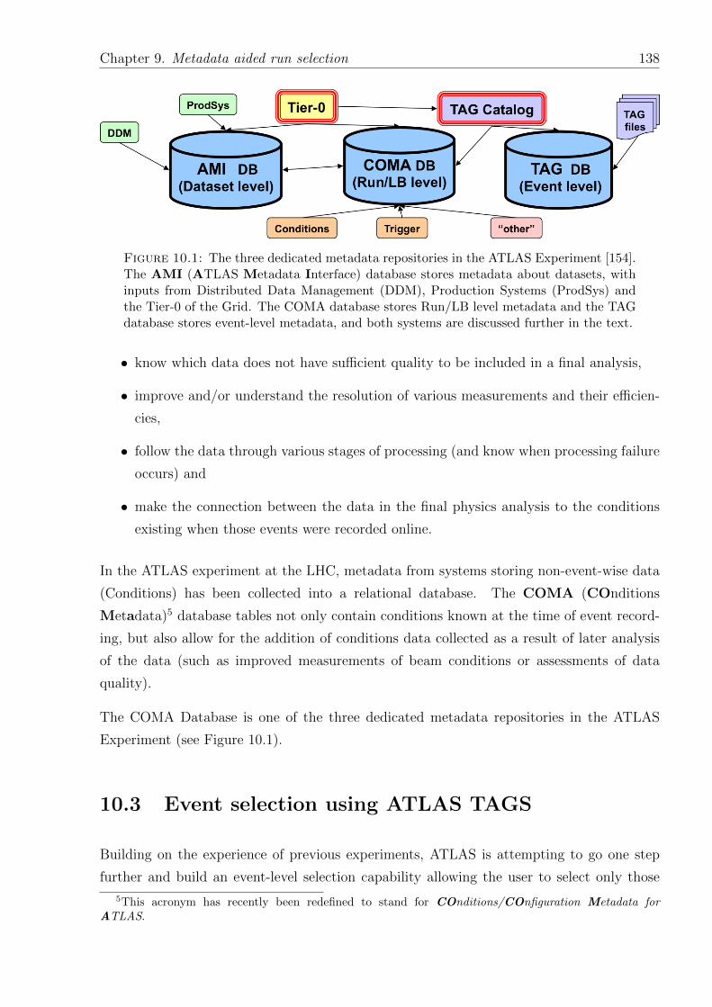
Chapter 9. Metadata aided run selection 138
Figure 10.1: The three dedicated metadata repositories in the ATLAS Experiment [154].The AMI (ATLAS Metadata Interface) database stores metadata about datasets, withinputs from Distributed Data Management (DDM), Production Systems (ProdSys) andthe Tier-0 of the Grid. The COMA database stores Run/LB level metadata and the TAGdatabase stores event-level metadata, and both systems are discussed further in the text.
• know which data does not have sufficient quality to be included in a final analysis,
• improve and/or understand the resolution of various measurements and their efficien-
cies,
• follow the data through various stages of processing (and know when processing failure
occurs) and
• make the connection between the data in the final physics analysis to the conditions
existing when those events were recorded online.
In the ATLAS experiment at the LHC, metadata from systems storing non-event-wise data
(Conditions) has been collected into a relational database. The COMA (COnditions
Metadata)5 database tables not only contain conditions known at the time of event record-
ing, but also allow for the addition of conditions data collected as a result of later analysis
of the data (such as improved measurements of beam conditions or assessments of data
quality).
The COMA Database is one of the three dedicated metadata repositories in the ATLAS
Experiment (see Figure 10.1).
10.3 Event selection using ATLAS TAGS
Building on the experience of previous experiments, ATLAS is attempting to go one step
further and build an event-level selection capability allowing the user to select only those
5This acronym has recently been redefined to stand for COnditions/COnfiguration Metadata forATLAS.
Chapter 9. Metadata aided run selection 139
events which are of particular interest. The RAW data collected by the ATLAS detector
is passed through various stages of processing in order to produce slimmed and compact
data sets which contain only those variables essential to the end user. The final smallest
files produced, TAGs, are produced for each event and contain all of the variables needed to
make an event selection. When a user runs their analysis code using TAGs on the Grid, the
software will find the original larger data set in order to access all of the required data.
ELSSI (Event Level Selection Service Interface) [155] allows users to make an event level
selection based on TAGs. Selection can be made using criteria, stored at the event level,
such as physics stream, run number, triggers and physics objects in the event.
But many run-level selections, such as conditions of data taking and processing, are outside
the scope of event level selections because that data is not stored event-by-event. So, a
run-level selection system is needed.
10.4 runBrowser - Dynamic metadata aided Run se-
lection
The ATLAS metadata infrastructure has been designed to facilitate logical and efficient
access to all flavors of analysis. The runBrowser interface [155], shown in Figure 10.2, allows
users to select Runs based on all available conditions data and conditions metadata. A flow
diagram of their dependencies is shown in Figure 10.3. The target audience of the interface
ranges from those who are not aware of exactly what data is available (and therefore a
dynamic selection interface gives transparency) to the expert user who wants full flexibility
to select a precise combination of Luminosity Blocks based on all available information.
The bulk of the browser is coded using PHP, interfaced with HTML and CSS. Faced with the
challenge of allowing selection from such a large pool of information, we employ JavaScript
and jQuery to develop the ‘ergonomics’ of the interface. Although a first version has now
been put into production, there are still many plans for further development - this is discussed
in section 10.5.
The main page consists of multiple expandable sections: one for each selection criteria.
Using jQuery, the user may collapse and expand each section to reveal the values which are
available for selection. In most cases these values are in the form of a table. Values are
retrieved from the database using SQL queries which are built using PHP. For some criteria,
a text box alternative is included allowing the use of ranges and wild-cards - for example, a
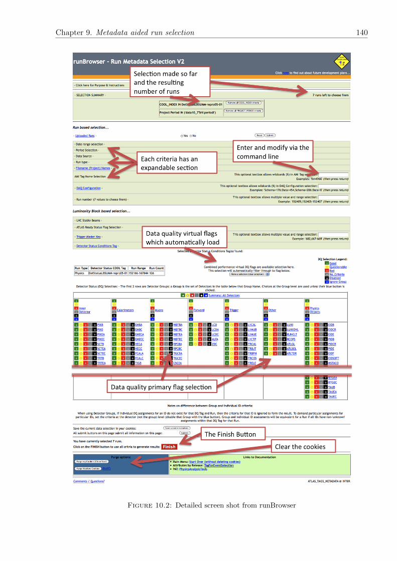
Chapter 9. Metadata aided run selection 140
Figure 10.2: Detailed screen shot from runBrowser
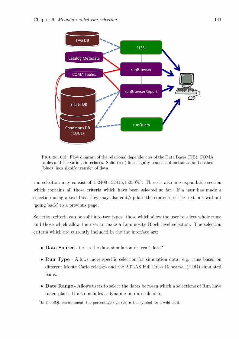
Chapter 9. Metadata aided run selection 141
Figure 10.3: Flow diagram of the relational dependencies of the Data Bases (DB), COMAtables and the various interfaces. Solid (red) lines signify transfer of metadata and dashed(blue) lines signify transfer of data.
run selection may consist of 152409-152415,15250%6. There is also one expandable section
which contains all those criteria which have been selected so far. If a user has made a
selection using a text box, they may also edit/update the contents of the text box without
‘going back’ to a previous page.
Selection criteria can be split into two types: those which allow the user to select whole runs;
and those which allow the user to make a Luminosity Block level selection. The selection
criteria which are currently included in the the interface are:
• Data Source - i.e. Is the data simulation or ‘real’ data?
• Run Type - Allows more specific selection for simulation data: e.g. runs based on
different Monte Carlo releases and the ATLAS Full Dress Rehearsal (FDR) simulated
Runs.
• Date Range - Allows users to select the dates between which a selections of Run have
taken place. It also includes a dynamic pop-up calendar.
6In the SQL environment, the percentage sign (%) is the symbol for a wild-card.

Chapter 9. Metadata aided run selection 142
• Period Selection - Periods are periods in time for which LHC configuration was
approximately stable. The periods are human defined and allow a convenient division
of the data into smaller, more manageable chunks.
• Filename (Project) Names - A further tag given to data. Examples include
‘data09 900GeV’ and ‘data10 7TeV’.
• Trigger Master Key7 - Each set of unique logical conditions imposed by the online
(or simulated) trigger system is assigned a unique integer ‘Trigger Super Master Key’.
runBrowser allows selection of one or more of these keys.
• DAQ Configuration - This is an online configuration tag used by the Tier 0 - may be
useful to experts in a detector and TDAQ (Trigger & Data AcQuisition) commissioning.
• Detector Status Conditions Tag8 - Detector Status (Data Quality) is assessed on
a Run/Luminosity Block level by experts. When a set of DQ assessments becomes
official, that set is assigned a unique tag in the ATLAS Conditions Database called a
‘Conditions Tag’.
• Run Number - This table shows the runs which fit all of the selection criteria so
far. With each Run are associated links to run specific information on AMI9 [156],
runQuery (see section 10.2) and a separate interface to the trigger database [157].
The table also includes a link to the runBrowser Run Report for each run. This
report contains a concise compilation of the information contained within the COMA
tables. This information currently includes general Run conditions, load status, debug
information, DQ assessments, prescale evolution and trigger information.
• Current status of TAG availability - This Yes/No selection allows the user to select
Runs which are available, via the ELSSI browser, to the TAG DB: Current policy is to
keep only the 2 latest processing of Runs available in the TAG database- this directs
the user to the latest/best data and conserves database resources to optimize that
access.
Help and documentation is available throughout the interface in the form of pop-up windows,
an expandable section containing ‘Purpose and Instructions’ and short strings of text which
appear when the cursor hovers over certain objects.
7Selection of a Trigger Master Key then allows further selection of the Level 1 and High Level Trigger(HLT) prescales.
8Selection of a Detector Status Condition Tag then allows further selection of individual detector flags(shown in Figure 10.2). It is also possible to choose from a list of pre-prescribed ‘Virtual Flags’ [135] which,using JavaScript, automatically set each of the individual detector flags to the correct position.
9AMI is a cataloging system using the Tier 0 database and production database in order to displayinformation about all of the registered ATLAS datasets.
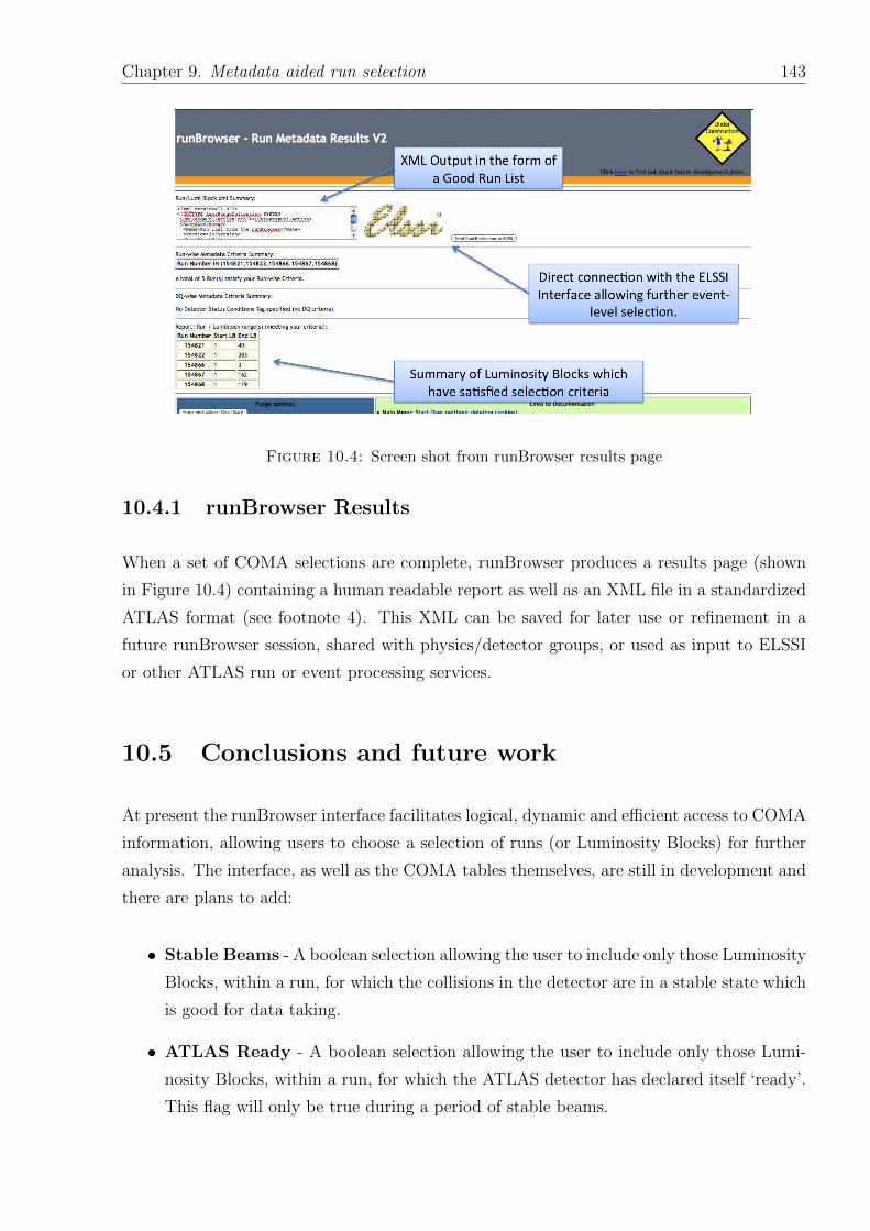
Chapter 9. Metadata aided run selection 143
Figure 10.4: Screen shot from runBrowser results page
10.4.1 runBrowser Results
When a set of COMA selections are complete, runBrowser produces a results page (shown
in Figure 10.4) containing a human readable report as well as an XML file in a standardized
ATLAS format (see footnote 4). This XML can be saved for later use or refinement in a
future runBrowser session, shared with physics/detector groups, or used as input to ELSSI
or other ATLAS run or event processing services.
10.5 Conclusions and future work
At present the runBrowser interface facilitates logical, dynamic and efficient access to COMA
information, allowing users to choose a selection of runs (or Luminosity Blocks) for further
analysis. The interface, as well as the COMA tables themselves, are still in development and
there are plans to add:
• Stable Beams - A boolean selection allowing the user to include only those Luminosity
Blocks, within a run, for which the collisions in the detector are in a stable state which
is good for data taking.
• ATLAS Ready - A boolean selection allowing the user to include only those Lumi-
nosity Blocks, within a run, for which the ATLAS detector has declared itself ‘ready’.
This flag will only be true during a period of stable beams.

Chapter 9. Metadata aided run selection 144
• Specific Magnet Information - the status of the ATLAS toroid and solenoid.
• Also other information concerning Luminosity, triggers and data streams.
Appendix A
Determination of binning in χ and mjj
A.1 Determination of binning in χ
The fine χ binning is determined by considering the purity and stability of bin migrations
in χ. These quantities are designed to quantify the bin migrations when going from truth
level information to fully-reconstructed simulation level. These quantities are defined as
Purityij =Nrec(i)&gen(j)
Nrec(i)
and Stabilityij =Nrec(i)&gen(j)
Ngen(j)
(A.1)
where Nrec(i)&gen(j) is, for a given Monte Carlo sample, the number of jets or events which
are placed in bin j using particle level truth information and are placed in bin i using
reconstruction-level data. Nrec is the total number of reconstructed entries in bin i and
Ngen(j) is the total number of entries using truth information in bin j. It is noted that∑j Purityij = 1 for all i and
∑i Stabilityij = 1 for all j. Using this prescription, the
optimal binning is achieved through a high bin Purityi=j and Stabilityi=j over the whole
range of χ.
Two further aspects to be considered are the ability to resolve the detailed shape of χ-spectra
at low χ (where new physics models predict an excess), and the typical cell granularity of
the ATLAS hadronic calorimetry (which is 0.1 in η for the Tile Calorimeter). In a previous
ATLAS study [138] it was found that small migrations of the jet axes due to the granularity
can be observed, which lead to a modulation of jet η-spectra with a periodicity of 0.1.
As migrations and the same periodicity result for η-differences, it is advisable to place the
borders of χ-bins at points of minimal migration to minimise the influence on χ spectra. It
145
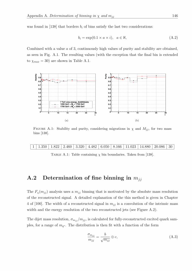
Appendix A. Determination of binning in χ and mjj 146
was found in [138] that borders bi of bins satisfy the last two considerations:
bi = exp(0.1× a× i), a ∈ ℵ, (A.2)
Combined with a value a of 3, continuously high values of purity and stability are obtained,
as seen in Fig. A.1. The resulting values (with the exception that the final bin is extended
to χmax = 30) are shown in Table A.1.
χ
5 10 15 20 25 30
Sta
bil
ity
0
0.1
0.2
0.3
0.4
0.5
0.6
0.7
0.8
0.9
1
7 TeV cms energy, AntiKt6Jets < 1700 GeV
jj1200 GeV < M
< 2500 GeVjj
1700 GeV < M
(a)
χ
5 10 15 20 25 30
Purity
0
0.1
0.2
0.3
0.4
0.5
0.6
0.7
0.8
0.9
1
(b)
Figure A.1: Stability and purity, considering migrations in χ and Mjj , for two massbins [138].
1 1.350 1.822 2.460 3.320 4.482 6.050 8.166 11.023 14.880 20.086 30
Table A.1: Table containing χ bin boundaries. Taken from [138].
A.2 Determination of fine binning in mjj
The Fχ(mjj) analysis uses a mjj binning that is motivated by the absolute mass resolution
of the reconstructed signal. A detailed explanation of the this method is given in Chapter
4 of [100]. The width of a reconstructed signal in mjj is a convolution of the intrinsic mass
width and the energy resolution of the two reconstructed jets (see Figure A.2).
The dijet mass resolution, σmjj/mjj, is calculated for fully-reconstructed excited quark sam-
ples, for a range of mq∗ . The distribution is then fit with a function of the form
σmjjmjj
=b√mjj
⊕ c, (A.3)
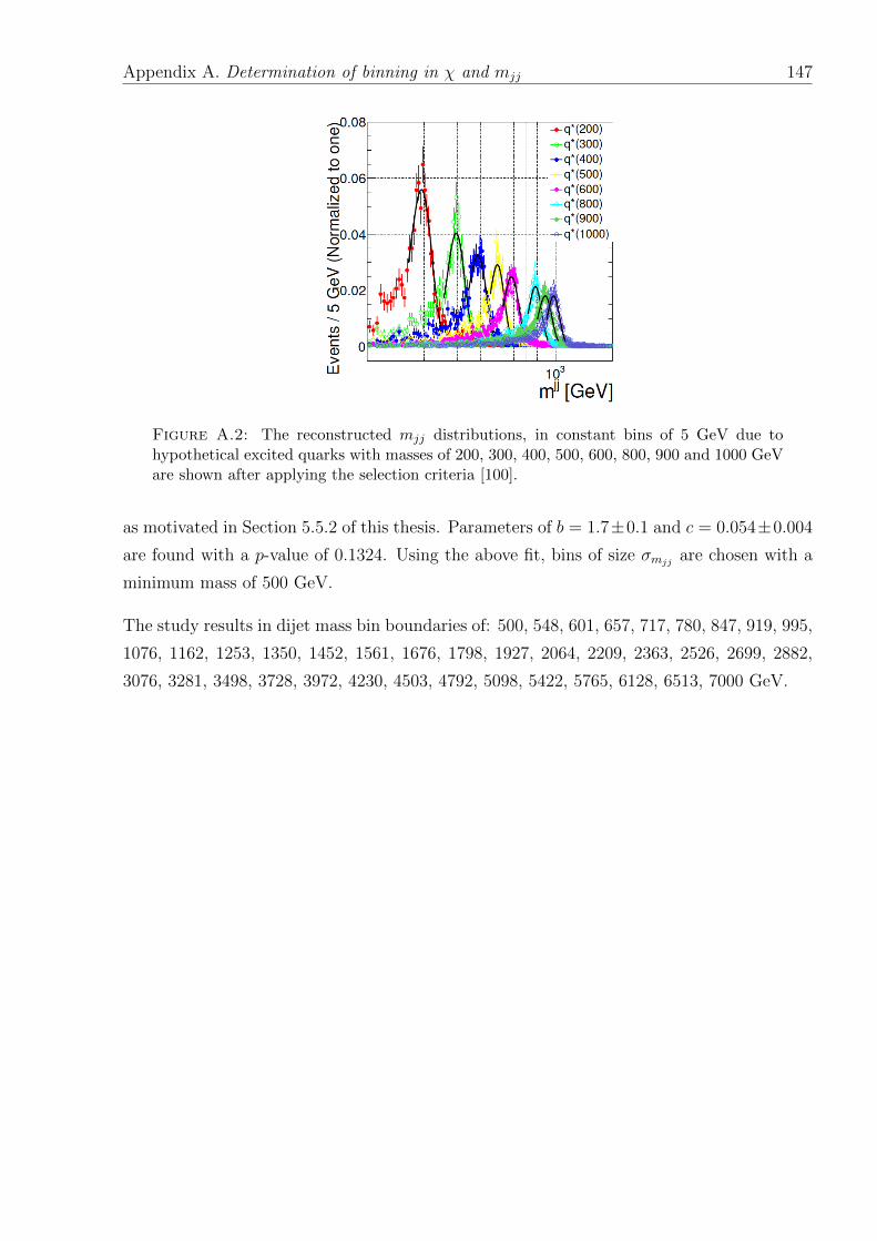
Appendix A. Determination of binning in χ and mjj 147
Figure A.2: The reconstructed mjj distributions, in constant bins of 5 GeV due tohypothetical excited quarks with masses of 200, 300, 400, 500, 600, 800, 900 and 1000 GeVare shown after applying the selection criteria [100].
as motivated in Section 5.5.2 of this thesis. Parameters of b = 1.7±0.1 and c = 0.054±0.004
are found with a p-value of 0.1324. Using the above fit, bins of size σmjj are chosen with a
minimum mass of 500 GeV.
The study results in dijet mass bin boundaries of: 500, 548, 601, 657, 717, 780, 847, 919, 995,
1076, 1162, 1253, 1350, 1452, 1561, 1676, 1798, 1927, 2064, 2209, 2363, 2526, 2699, 2882,
3076, 3281, 3498, 3728, 3972, 4230, 4503, 4792, 5098, 5422, 5765, 6128, 6513, 7000 GeV.
Appendix B
Comparing ATLFAST II to Geant
full simulation
The full 2011 dataset, with an integrated luminosity of 4.8 fb−1represents a substantial
increase over 2010, and has greatly decreased the statistical uncertainties in data distribu-
tions. This necessitates a corresponding increase in the size of MC samples, to prevent MC
statistical fluctuations from becoming a dominant source of uncertainty in dijet mass and
angular analyses. Full simulation of events using GEANT4 is time intensive, and the avail-
able Grid capacity does not allow for the processing of larger fully-simulated MC samples
on the timescales required for publication of results.
The ATLFAST II [65] program, which employs FastCaloSim [66] for calorimeter simulation,
typically runs one order of magnitude faster than Geant, and is in the process of becoming
the new default for MC full simulation. To validate this new procedure, MC truth samples
have been passed through ATLFAST II detector simulation and compared to Geant full
simulation of the same samples.
Pythia 6 dijet event samples are typically generated in broad bins of partonic pT . The
Geant samples have J0-J8, with 2.8 million events for J3 through J6, and 1.4 million each
in J7 and J8. In order to increase the statistics for the angular distributions, the ATLFAST
II samples have the partonic range of J7 split into two halves; J7a from 1120 to 1680 GeV
and J7b from 1680 to 2240 GeV. The ATLFAST II samples have 1.4 million events for J0-J3
and for J7, J7a and J7b, and 2.8 million events for J4-J6 and J8. Note that in order to
avoid double counting the J7 cross section, all weights of the J7(a/b) samples get a factor
0.5. Each simulation comes with its own set of calibration constants.
148
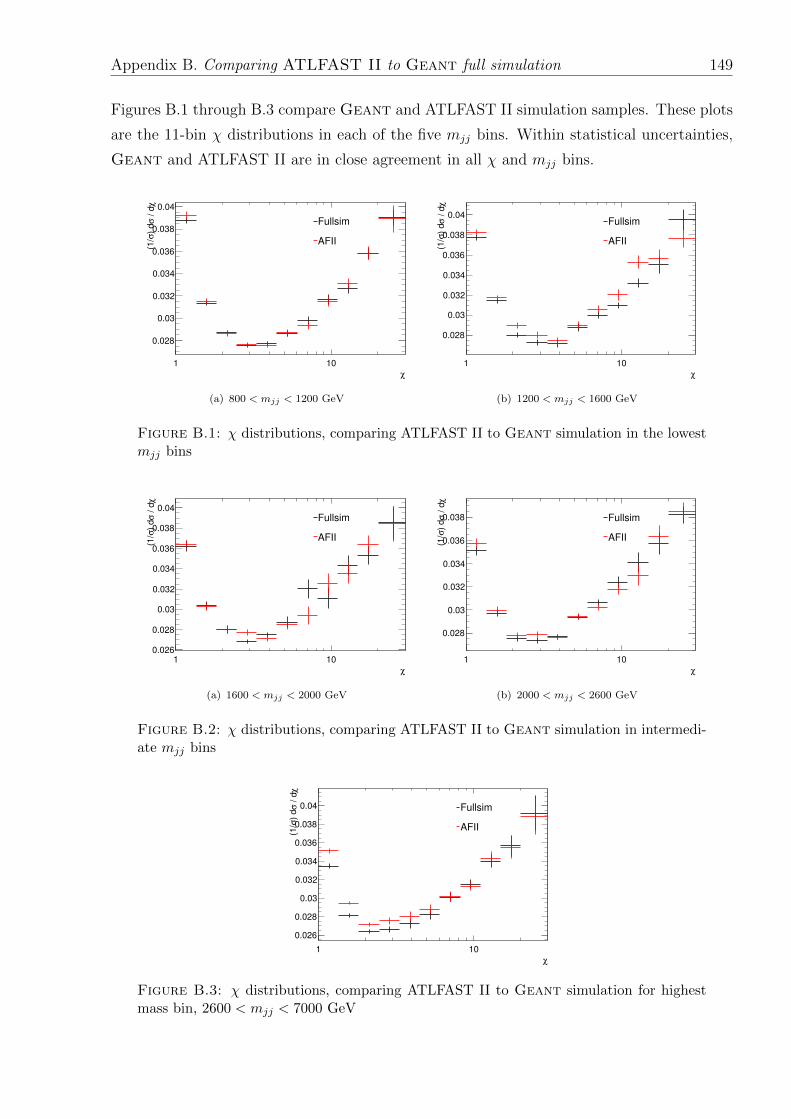
Appendix B. Comparing ATLFAST II to Geant full simulation 149
Figures B.1 through B.3 compare Geant and ATLFAST II simulation samples. These plots
are the 11-bin χ distributions in each of the five mjj bins. Within statistical uncertainties,
Geant and ATLFAST II are in close agreement in all χ and mjj bins.
χ
1 10
χ / d
σ)
dσ
(1/
0.028
0.03
0.032
0.034
0.036
0.038
0.04
Fullsim
AFII
(a) 800 < mjj < 1200 GeV
χ
1 10
χ / d
σ)
dσ
(1/
0.028
0.03
0.032
0.034
0.036
0.038
0.04Fullsim
AFII
(b) 1200 < mjj < 1600 GeV
Figure B.1: χ distributions, comparing ATLFAST II to Geant simulation in the lowestmjj bins
χ
1 10
χ / d
σ)
dσ
(1/
0.026
0.028
0.03
0.032
0.034
0.036
0.038
0.04Fullsim
AFII
(a) 1600 < mjj < 2000 GeV
χ
1 10
χ / d
σ)
dσ
(1/
0.028
0.03
0.032
0.034
0.036
0.038 Fullsim
AFII
(b) 2000 < mjj < 2600 GeV
Figure B.2: χ distributions, comparing ATLFAST II to Geant simulation in intermedi-ate mjj bins
χ
1 10
χ / d
σ)
dσ
(1/
0.026
0.028
0.03
0.032
0.034
0.036
0.038
0.04 Fullsim
AFII
Figure B.3: χ distributions, comparing ATLFAST II to Geant simulation for highestmass bin, 2600 < mjj < 7000 GeV
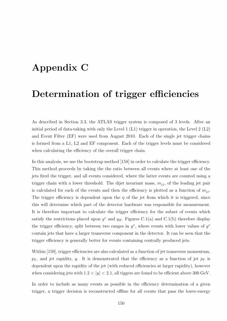
Appendix C
Determination of trigger efficiencies
As described in Section 3.3, the ATLAS trigger system is composed of 3 levels. After an
initial period of data-taking with only the Level 1 (L1) trigger in operation, the Level 2 (L2)
and Event Filter (EF) were used from August 2010. Each of the single jet trigger chains
is formed from a L1, L2 and EF component. Each of the trigger levels must be considered
when calculating the efficiency of the overall trigger chain.
In this analysis, we use the bootstrap method [158] in order to calculate the trigger efficiency.
This method proceeds by taking the the ratio between all events where at least one of the
jets fired the trigger, and all events considered, where the latter events are counted using a
trigger chain with a lower threshold. The dijet invariant mass, mjj, of the leading jet pair
is calculated for each of the events and then the efficiency is plotted as a function of mjj.
The trigger efficiency is dependent upon the η of the jet from which it is triggered, since
this will determine which part of the detector hardware was responsible for measurement.
It is therefore important to calculate the trigger efficiency for the subset of events which
satisfy the restrictions placed upon y∗ and yB. Figures C.1(a) and C.1(b) therefore display
the trigger efficiency, split between two ranges in y∗, where events with lower values of y∗
contain jets that have a larger transverse component in the detector. It can be seen that the
trigger efficiency is generally better for events containing centrally produced jets.
Within [159], trigger efficiencies are also calculated as a function of jet transverse momentum,
pT , and jet rapidity, y. It is demonstrated that the efficiency as a function of jet pT is
dependent upon the rapidity of the jet (with reduced efficiencies at larger rapidity), however
when considering jets with 1.2 < |y| < 2.1, all tiggers are found to be efficient above 300 GeV.
In order to include as many events as possible in the efficiency determination of a given
trigger, a trigger decision is reconstructed offline for all events that pass the lower-energy
150

Appendix C. Determination of trigger efficiencies 151
reference trigger. A trigger decision can be determined by looking at the energy recorded
at level 1, level 2 and the event filter, and requiring that the energy at each trigger level is
above the required threshold.
Although the above method is constrained to the number of events passing the reference trig-
ger (after prescale), the statistics are sufficient to construct the efficiency curves in Figure C.1
as a function of mjj.
By zooming into these plots, one is able to determine that value of mjj above which the
efficiency is > 99%, which is an ATLAS convention for trigger efficiency requirements.
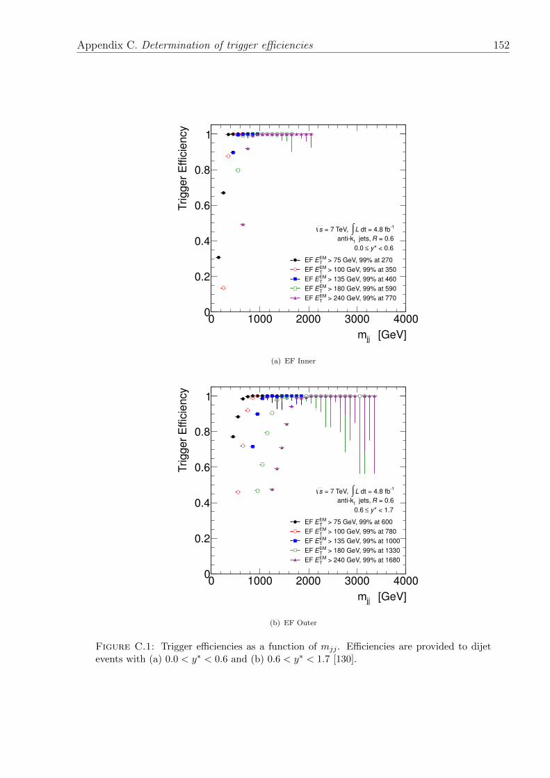
Appendix C. Determination of trigger efficiencies 152
[GeV]jjm
0 1000 2000 3000 4000
Trigger
Effic
iency
0
0.2
0.4
0.6
0.8
1
> 75 GeV, 99% at 270EMTEEF
> 100 GeV, 99% at 350EMTEEF
> 135 GeV, 99% at 460EMTEEF
> 180 GeV, 99% at 590EMTEEF
> 240 GeV, 99% at 770EMTEEF
1 dt = 4.8 fbL∫ = 7 TeV, s
= 0.6R jets, tantik
* < 0.6y ≤0.0
(a) EF Inner
[GeV]jjm
0 1000 2000 3000 4000
Trigger
Effic
iency
0
0.2
0.4
0.6
0.8
1
> 75 GeV, 99% at 600EMTEEF
> 100 GeV, 99% at 780EMTEEF
> 135 GeV, 99% at 1000EMTEEF
> 180 GeV, 99% at 1330EMTEEF
> 240 GeV, 99% at 1680EMTEEF
1 dt = 4.8 fbL∫ = 7 TeV, s
= 0.6R jets, tantik
* < 1.7y ≤0.6
(b) EF Outer
Figure C.1: Trigger efficiencies as a function of mjj . Efficiencies are provided to dijetevents with (a) 0.0 < y∗ < 0.6 and (b) 0.6 < y∗ < 1.7 [130].
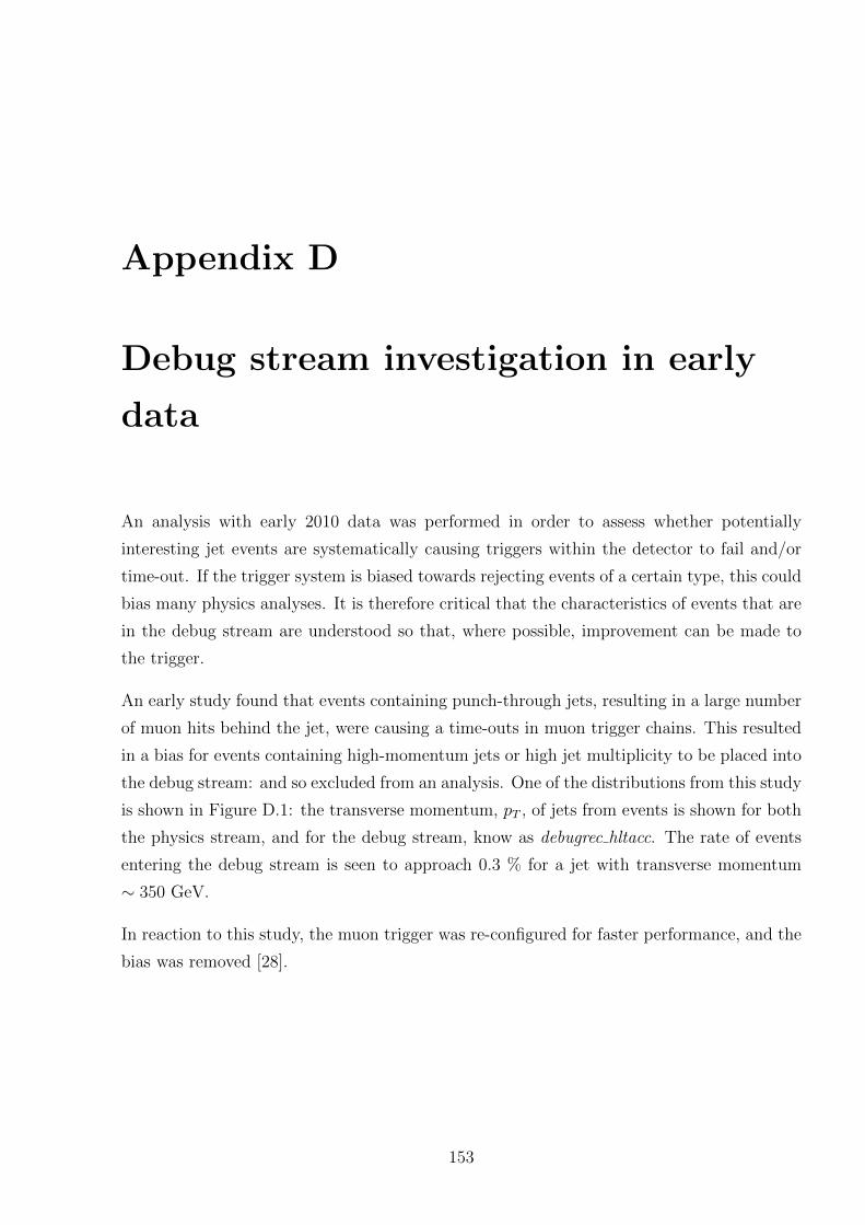
Appendix D
Debug stream investigation in early
data
An analysis with early 2010 data was performed in order to assess whether potentially
interesting jet events are systematically causing triggers within the detector to fail and/or
time-out. If the trigger system is biased towards rejecting events of a certain type, this could
bias many physics analyses. It is therefore critical that the characteristics of events that are
in the debug stream are understood so that, where possible, improvement can be made to
the trigger.
An early study found that events containing punch-through jets, resulting in a large number
of muon hits behind the jet, were causing a time-outs in muon trigger chains. This resulted
in a bias for events containing high-momentum jets or high jet multiplicity to be placed into
the debug stream: and so excluded from an analysis. One of the distributions from this study
is shown in Figure D.1: the transverse momentum, pT , of jets from events is shown for both
the physics stream, and for the debug stream, know as debugrec hltacc. The rate of events
entering the debug stream is seen to approach 0.3 % for a jet with transverse momentum
∼ 350 GeV.
In reaction to this study, the muon trigger was re-configured for faster performance, and the
bias was removed [28].
153
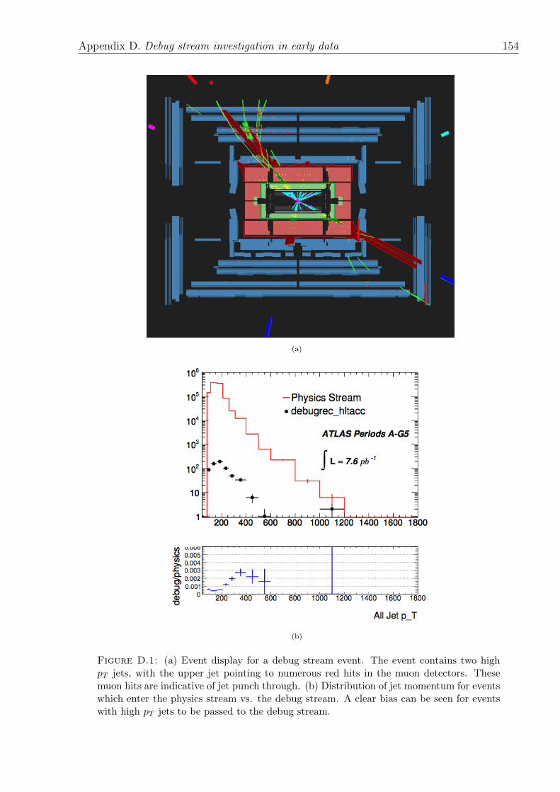
Appendix D. Debug stream investigation in early data 154
(a)
(b)
Figure D.1: (a) Event display for a debug stream event. The event contains two highpT jets, with the upper jet pointing to numerous red hits in the muon detectors. Thesemuon hits are indicative of jet punch through. (b) Distribution of jet momentum for eventswhich enter the physics stream vs. the debug stream. A clear bias can be seen for eventswith high pT jets to be passed to the debug stream.
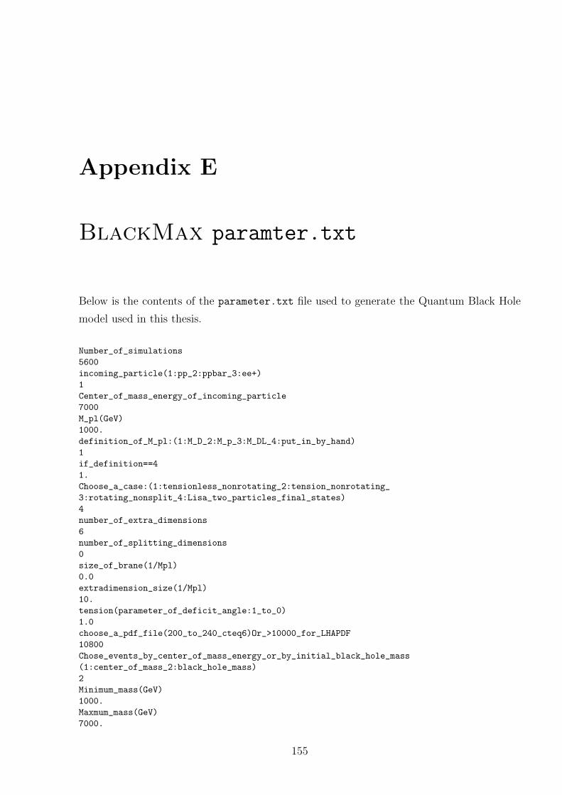
Appendix E
BlackMax paramter.txt
Below is the contents of the parameter.txt file used to generate the Quantum Black Hole
model used in this thesis.
Number_of_simulations
5600
incoming_particle(1:pp_2:ppbar_3:ee+)
1
Center_of_mass_energy_of_incoming_particle
7000
M_pl(GeV)
1000.
definition_of_M_pl:(1:M_D_2:M_p_3:M_DL_4:put_in_by_hand)
1
if_definition==4
1.
Choose_a_case:(1:tensionless_nonrotating_2:tension_nonrotating_
3:rotating_nonsplit_4:Lisa_two_particles_final_states)
4
number_of_extra_dimensions
6
number_of_splitting_dimensions
0
size_of_brane(1/Mpl)
0.0
extradimension_size(1/Mpl)
10.
tension(parameter_of_deficit_angle:1_to_0)
1.0
choose_a_pdf_file(200_to_240_cteq6)Or_>10000_for_LHAPDF
10800
Chose_events_by_center_of_mass_energy_or_by_initial_black_hole_mass
(1:center_of_mass_2:black_hole_mass)
2
Minimum_mass(GeV)
1000.
Maxmum_mass(GeV)
7000.
155
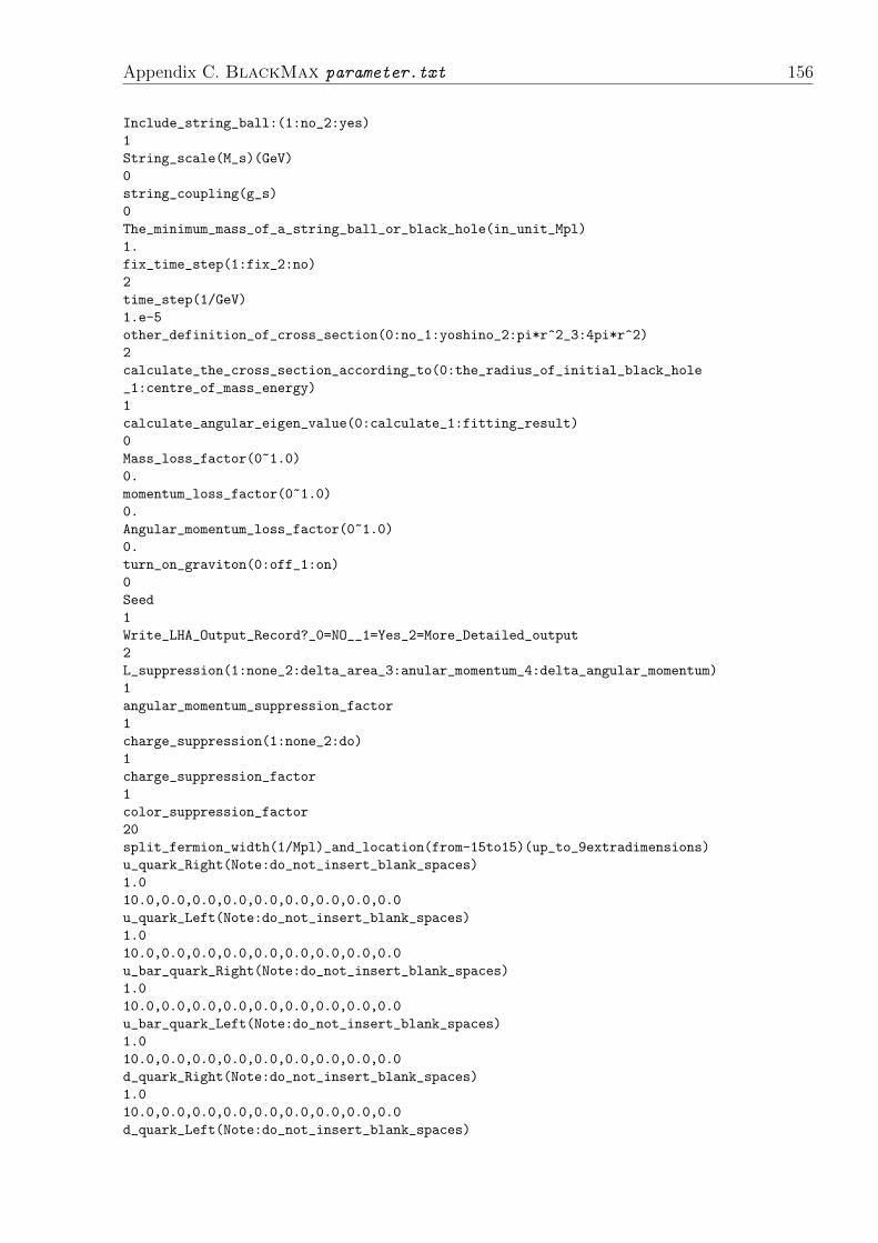
Appendix C. BlackMax parameter.txt 156
Include_string_ball:(1:no_2:yes)
1
String_scale(M_s)(GeV)
0
string_coupling(g_s)
0
The_minimum_mass_of_a_string_ball_or_black_hole(in_unit_Mpl)
1.
fix_time_step(1:fix_2:no)
2
time_step(1/GeV)
1.e-5
other_definition_of_cross_section(0:no_1:yoshino_2:pi*r^2_3:4pi*r^2)
2
calculate_the_cross_section_according_to(0:the_radius_of_initial_black_hole
_1:centre_of_mass_energy)
1
calculate_angular_eigen_value(0:calculate_1:fitting_result)
0
Mass_loss_factor(0~1.0)
0.
momentum_loss_factor(0~1.0)
0.
Angular_momentum_loss_factor(0~1.0)
0.
turn_on_graviton(0:off_1:on)
0
Seed
1
Write_LHA_Output_Record?_0=NO__1=Yes_2=More_Detailed_output
2
L_suppression(1:none_2:delta_area_3:anular_momentum_4:delta_angular_momentum)
1
angular_momentum_suppression_factor
1
charge_suppression(1:none_2:do)
1
charge_suppression_factor
1
color_suppression_factor
20
split_fermion_width(1/Mpl)_and_location(from-15to15)(up_to_9extradimensions)
u_quark_Right(Note:do_not_insert_blank_spaces)
1.0
10.0,0.0,0.0,0.0,0.0,0.0,0.0,0.0,0.0
u_quark_Left(Note:do_not_insert_blank_spaces)
1.0
10.0,0.0,0.0,0.0,0.0,0.0,0.0,0.0,0.0
u_bar_quark_Right(Note:do_not_insert_blank_spaces)
1.0
10.0,0.0,0.0,0.0,0.0,0.0,0.0,0.0,0.0
u_bar_quark_Left(Note:do_not_insert_blank_spaces)
1.0
10.0,0.0,0.0,0.0,0.0,0.0,0.0,0.0,0.0
d_quark_Right(Note:do_not_insert_blank_spaces)
1.0
10.0,0.0,0.0,0.0,0.0,0.0,0.0,0.0,0.0
d_quark_Left(Note:do_not_insert_blank_spaces)
Appendix C. BlackMax parameter.txt 157
1.0
10.0,0.0,0.0,0.0,0.0,0.0,0.0,0.0,0.0
d_bar_quark_Right(Note:do_not_insert_blank_spaces)
1.0
10.0,0.0,0.0,0.0,0.0,0.0,0.0,0.0,0.0
d_bar_quark_Left(Note:do_not_insert_blank_spaces)
1.0
10.0,0.0,0.0,0.0,0.0,0.0,0.0,0.0,0.0
s_quark_Right(Note:do_not_insert_blank_spaces)
1.0
10.0,0.0,0.0,0.0,0.0,0.0,0.0,0.0,0.0
s_quark_Left(Note:do_not_insert_blank_spaces)
1.0
10.0,0.0,0.0,0.0,0.0,0.0,0.0,0.0,0.0
s_bar_quark_Right(Note:do_not_insert_blank_spaces)
1.0
10.0,0.0,0.0,0.0,0.0,0.0,0.0,0.0,0.0
s_bar_quark_Left(Note:do_not_insert_blank_spaces)
1.0
10.0,0.0,0.0,0.0,0.0,0.0,0.0,0.0,0.0
c_quark_Right(Note:do_not_insert_blank_spaces)
1.0
10.0,0.0,0.0,0.0,0.0,0.0,0.0,0.0,0.0
c_quark_Left(Note:do_not_insert_blank_spaces)
1.0
10.0,0.0,0.0,0.0,0.0,0.0,0.0,0.0,0.0
c_bar_quark_Right(Note:do_not_insert_blank_spaces)
1.0
10.0,0.0,0.0,0.0,0.0,0.0,0.0,0.0,0.0
c_bar_quark_Left(Note:do_not_insert_blank_spaces)
1.0
10.0,0.0,0.0,0.0,0.0,0.0,0.0,0.0,0.0
b_quark_Right(Note:do_not_insert_blank_spaces)
1.0
10.0,0.0,0.0,0.0,0.0,0.0,0.0,0.0,0.0
b_quark_Left(Note:do_not_insert_blank_spaces)
1.0
10.0,0.0,0.0,0.0,0.0,0.0,0.0,0.0,0.0
b_bar_quark_Right(Note:do_not_insert_blank_spaces)
1.0
10.0,0.0,0.0,0.0,0.0,0.0,0.0,0.0,0.0
b_bar_quark_Left(Note:do_not_insert_blank_spaces)
1.0
10.0,0.0,0.0,0.0,0.0,0.0,0.0,0.0,0.0
t_quark_Right(Note:do_not_insert_blank_spaces)
1.0
10.0,0.0,0.0,0.0,0.0,0.0,0.0,0.0,0.0
t_quark_Left(Note:do_not_insert_blank_spaces)
1.0
10.0,0.0,0.0,0.0,0.0,0.0,0.0,0.0,0.0
t_bar_quark_Right(Note:do_not_insert_blank_spaces)
1.0
10.0,0.0,0.0,0.0,0.0,0.0,0.0,0.0,0.0
t_bar_quark_Left(Note:do_not_insert_blank_spaces)
1.0
10.0,0.0,0.0,0.0,0.0,0.0,0.0,0.0,0.0
e_-_Left(Note:do_not_insert_blank_spaces)
1.0
Appendix C. BlackMax parameter.txt 158
-10.0,0.0,0.0,0.0,0.0,0.0,0.0,0.0,0.0
e_-_Right(Note:do_not_insert_blank_spaces)
1.0
-10.0,0.0,0.0,0.0,0.0,0.0,0.0,0.0,0.0
e_+_Left(Note:do_not_insert_blank_spaces)
1.0
-10.0,0.0,0.0,0.0,0.0,0.0,0.0,0.0,0.0
e_+_Right(Note:do_not_insert_blank_spaces)
1.0
-10.0,0.0,0.0,0.0,0.0,0.0,0.0,0.0,0.0
mu_-_Left(Note:do_not_insert_blank_spaces)
1.0
-10.0,0.0,0.0,0.0,0.0,0.0,0.0,0.0,0.0
mu_-_Right(Note:do_not_insert_blank_spaces)
1.0
-10.0,0.0,0.0,0.0,0.0,0.0,0.0,0.0,0.0
mu_+_Left(Note:do_not_insert_blank_spaces)
1.0
-10.0,0.0,0.0,0.0,0.0,0.0,0.0,0.0,0.0
mu_+_Right(Note:do_not_insert_blank_spaces)
1.0
-10.0,0.0,0.0,0.0,0.0,0.0,0.0,0.0,0.0
tau_-_Left(Note:do_not_insert_blank_spaces)
1.0
-10.0,0.0,0.0,0.0,0.0,0.0,0.0,0.0,0.0
tau_-_Right(Note:do_not_insert_blank_spaces)
1.0
-10.0,0.0,0.0,0.0,0.0,0.0,0.0,0.0,0.0
tau_+_Left(Note:do_not_insert_blank_spaces)
1.0
-10.0,0.0,0.0,0.0,0.0,0.0,0.0,0.0,0.0
tau_+_Right(Note:do_not_insert_blank_spaces)
1.0
-10.0,0.0,0.0,0.0,0.0,0.0,0.0,0.0,0.0
nutrino_e-(Note:do_not_insert_blank_spaces)
1.0
-10.0,0.0,0.0,0.0,0.0,0.0,0.0,0.0,0.0
nutrino_e+(Note:do_not_insert_blank_spaces)
1.0
-10.0,0.0,0.0,0.0,0.0,0.0,0.0,0.0,0.0
nutrino_mu-(Note:do_not_insert_blank_spaces)
1.0
-10.0,0.0,0.0,0.0,0.0,0.0,0.0,0.0,0.0
nutrino_mu+(Note:do_not_insert_blank_spaces)
1.0
-10.0,0.0,0.0,0.0,0.0,0.0,0.0,0.0,0.0
nutrino_tau-(Note:do_not_insert_blank_spaces)
1.0
-10.0,0.0,0.0,0.0,0.0,0.0,0.0,0.0,0.0
nutrino_tau+(Note:do_not_insert_blank_spaces)
1.0
-10.0,0.0,0.0,0.0,0.0,0.0,0.0,0.0,0.0
number_of_conservation
1
d,s,b,u,c,t,e,mu,tau,nu_e,nu_mu,nu_tau
1,1,1,1,1,1,0,0,0,0,0,0
1,1,1,1,1,1,-3,-3,-3,-3,-3,-3
0,0,0,0,0,0,1,1,1,1,1,1

Appendix C. BlackMax parameter.txt 159
0,0,0,0,0,0,0,0,0,0,0,0
0,0,0,0,0,0,0,0,0,0,0,0
0,0,0,0,0,0,0,0,0,0,0,0
0,0,0,0,0,0,0,0,0,0,0,0
0,0,0,0,0,0,0,0,0,0,0,0
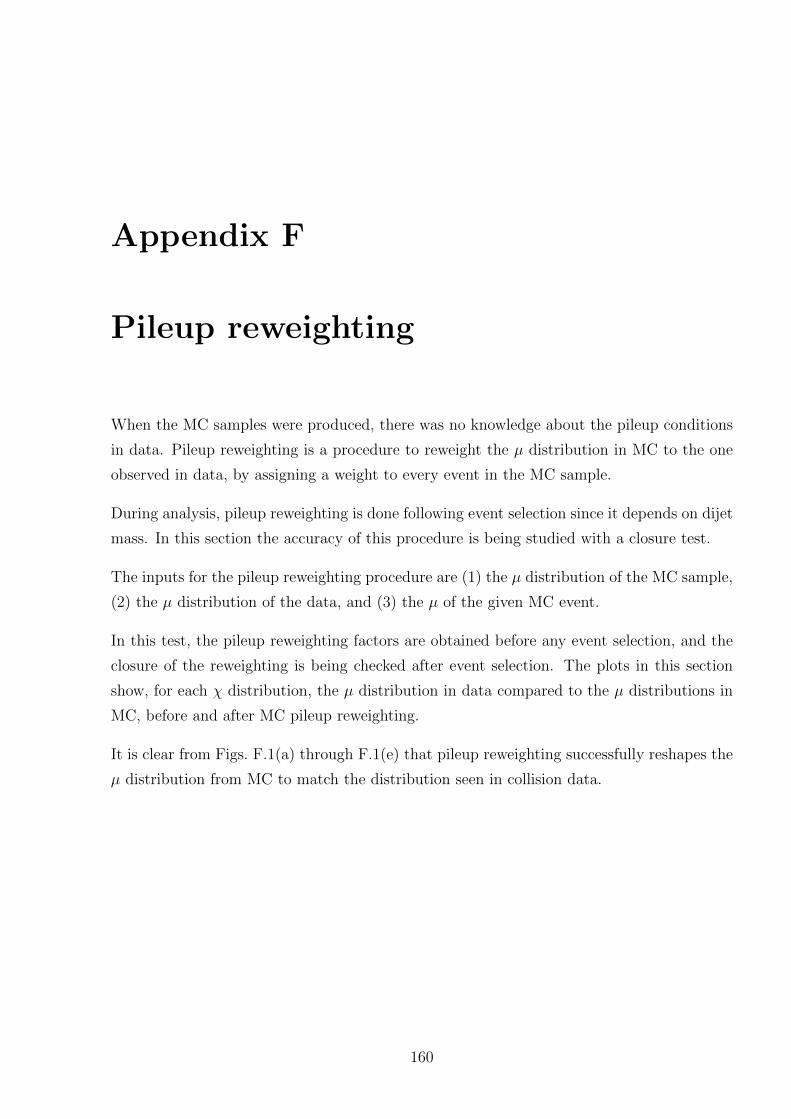
Appendix F
Pileup reweighting
When the MC samples were produced, there was no knowledge about the pileup conditions
in data. Pileup reweighting is a procedure to reweight the µ distribution in MC to the one
observed in data, by assigning a weight to every event in the MC sample.
During analysis, pileup reweighting is done following event selection since it depends on dijet
mass. In this section the accuracy of this procedure is being studied with a closure test.
The inputs for the pileup reweighting procedure are (1) the µ distribution of the MC sample,
(2) the µ distribution of the data, and (3) the µ of the given MC event.
In this test, the pileup reweighting factors are obtained before any event selection, and the
closure of the reweighting is being checked after event selection. The plots in this section
show, for each χ distribution, the µ distribution in data compared to the µ distributions in
MC, before and after MC pileup reweighting.
It is clear from Figs. F.1(a) through F.1(e) that pileup reweighting successfully reshapes the
µ distribution from MC to match the distribution seen in collision data.
160
Appendix D. Pileup reweighting 161
>µ<2 4 6 8 10 12 14 16 18 20
Norm
aliz
ed e
ntr
ies
0
0.05
0.1
0.15
0.2
0.25Pileup reweighting
=7 TeVs, 1
dt = 4.8 fbL∫
< 1200 GeVjj
800 GeV < m
Data
QCD
QCD, reweighted
(a) 800 GeV < mjj < 1200 GeV.
>µ<2 4 6 8 10 12 14 16 18 20
Norm
aliz
ed e
ntr
ies
0
0.05
0.1
0.15
0.2
0.25Pileup reweighting
=7 TeVs, 1
dt = 4.8 fbL∫
< 1600 GeVjj
1200 GeV < m
Data
QCD
QCD, reweighted
(b) 1200 GeV < mjj < 1600 GeV.
>µ<2 4 6 8 10 12 14 16 18 20
Norm
aliz
ed e
ntr
ies
0
0.05
0.1
0.15
0.2
0.25
0.3
0.35
0.4
Pileup reweighting
=7 TeVs, 1
dt = 4.8 fbL∫
< 2000 GeVjj
1600 GeV < m
Data
QCD
QCD, reweighted
(c) 1600 GeV < mjj < 2000 GeV.
>µ<2 4 6 8 10 12 14 16 18 20
Norm
aliz
ed e
ntr
ies
0
0.05
0.1
0.15
0.2
0.25Pileup reweighting
=7 TeVs, 1
dt = 4.8 fbL∫
< 2600 GeVjj
2000 GeV < m
Data
QCD
QCD, reweighted
(d) 2000 GeV < mjj < 2600 GeV.
>µ<2 4 6 8 10 12 14 16 18 20
Norm
aliz
ed e
ntr
ies
0
0.05
0.1
0.15
0.2
0.25Pileup reweighting
=7 TeVs, 1
dt = 4.8 fbL∫
< 7000 GeVjj
2600 GeV < m
Data
QCD
QCD, reweighted
(e) 2600 GeV < mjj < 7000 GeV.
Figure F.1: Effects of pile-up reweighing for all χ distributions.
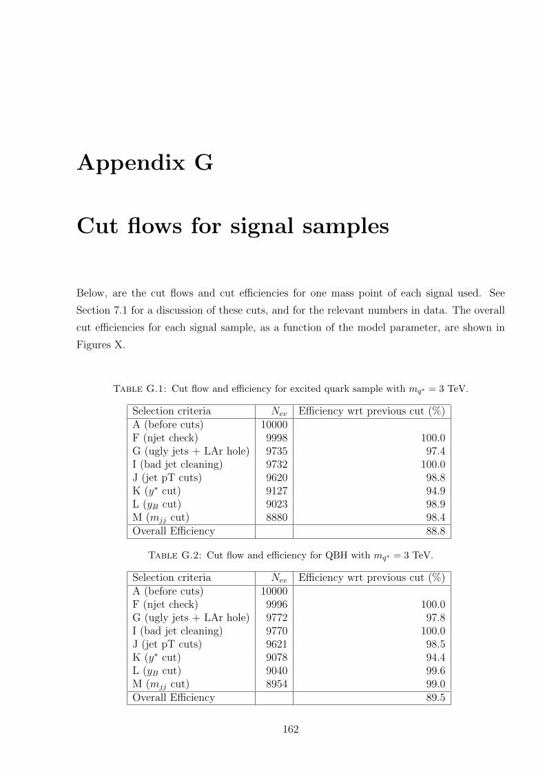
Appendix G
Cut flows for signal samples
Below, are the cut flows and cut efficiencies for one mass point of each signal used. See
Section 7.1 for a discussion of these cuts, and for the relevant numbers in data. The overall
cut efficiencies for each signal sample, as a function of the model parameter, are shown in
Figures X.
Table G.1: Cut flow and efficiency for excited quark sample with mq∗ = 3 TeV.
Selection criteria Nev Efficiency wrt previous cut (%)A (before cuts) 10000F (njet check) 9998 100.0G (ugly jets + LAr hole) 9735 97.4I (bad jet cleaning) 9732 100.0J (jet pT cuts) 9620 98.8K (y∗ cut) 9127 94.9L (yB cut) 9023 98.9M (mjj cut) 8880 98.4Overall Efficiency 88.8
Table G.2: Cut flow and efficiency for QBH with mq∗ = 3 TeV.
Selection criteria Nev Efficiency wrt previous cut (%)A (before cuts) 10000F (njet check) 9996 100.0G (ugly jets + LAr hole) 9772 97.8I (bad jet cleaning) 9770 100.0J (jet pT cuts) 9621 98.5K (y∗ cut) 9078 94.4L (yB cut) 9040 99.6M (mjj cut) 8954 99.0Overall Efficiency 89.5
162
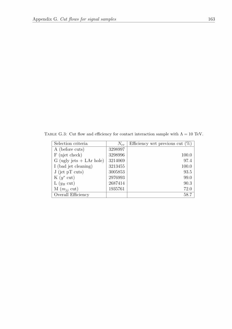
Appendix G. Cut flows for signal samples 163
Table G.3: Cut flow and efficiency for contact interaction sample with Λ = 10 TeV.
Selection criteria Nev Efficiency wrt previous cut (%)A (before cuts) 3298997F (njet check) 3298996 100.0G (ugly jets + LAr hole) 3214069 97.4I (bad jet cleaning) 3213455 100.0J (jet pT cuts) 3005853 93.5K (y∗ cut) 2976993 99.0L (yB cut) 2687414 90.3M (mjj cut) 1935761 72.0Overall Efficiency 58.7
Bibliography
[1] Lydon Evans and Philip Bryant (editors). Lhc machine. JINST, 3(S08001), 2008.
[2] Derek Greenwood W. Cottingham. An Introduction to the Standard Model of Particle
Physics. 1998.
[3] S.L. Glashow. Partial Symmetries of Weak Interactions. Nucl.Phys., 22:579–588, 1961.
doi: 10.1016/0029-5582(61)90469-2.
[4] Steven Weinberg. A model of leptons. Phys. Rev. Lett., 19:1264–1266, Nov
1967. doi: 10.1103/PhysRevLett.19.1264. URL http://link.aps.org/doi/10.1103/
PhysRevLett.19.1264.
[5] A. salam in elementary particle theory, n. svartholm, ed., almquist and wiksells, stock-
holm (1969), p. 367.
[6] S. L. Glashow, J. Iliopoulos, and L. Maiani. Weak interactions with lepton-hadron
symmetry. Phys. Rev. D, 2:1285–1292, Oct 1970. doi: 10.1103/PhysRevD.2.1285.
URL http://link.aps.org/doi/10.1103/PhysRevD.2.1285.
[7] Barton Zwiebach. A First Course in String Theory. CUP, 2009.
[8] K. Nakamura et al. The review of particle physics. J. Phys., G 37(075021), 2010.
[9] M. Gonzalez-Garcia, Michele Maltoni, and Jordi Salvado. Updated global fit to three
neutrino mixing: status of the hints of θ13 > 0. Journal of High Energy Physics, 2010:
1–20, 2010. ISSN 1029-8479. URL http://dx.doi.org/10.1007/JHEP04(2010)056.
10.1007/JHEP04(2010)056.
[10] Ian Brock and Thomas Schorner-Sadenius. Physics at the Terascale. Whiley, 2010.
[11] Stephen P. Martin. A Supersymmetry Primer. 1997.
[12] Christopher T. Hill and Elizabeth H. Simmons. Strong dynamics and electroweak
symmetry breaking. Physics Reports, 381(46):235 – 402, 2003. ISSN 0370-1573. doi:
164
Bibliography 165
10.1016/S0370-1573(03)00140-6. URL http://www.sciencedirect.com/science/
article/pii/S0370157303001406.
[13] The ATLAS Collaboration. Observation of a new particle in the search for the standard
model higgs boson with the atlas detector at the lhc. Physics Letters B, 716(1):
1 – 29, 2012. ISSN 0370-2693. doi: 10.1016/j.physletb.2012.08.020. URL http:
//www.sciencedirect.com/science/article/pii/S037026931200857X.
[14] The CMS Collaboration. Observation of a new boson at a mass of 125 gev with the
cms experiment at the lhc. (arXiv:1207.7235 [hep-ex]), .
[15] ATLAS Collaboration. A search for new physics in dijet mass and angular distributions
in pp collisions at√s = 7 tev with the atlas detector. New Journal of Physics, 13(5):
053044, 2011. URL http://stacks.iop.org/1367-2630/13/i=5/a=053044.
[16] R Buckingham, A Cooper-Sarkar, J Ferrando, C Issever, K Lohwasser, and S White-
head. Using the charge asymmetry in w+jet production as a new probe of parton
distribution functions in different kinematic regions at the lhc. Technical Report ATL-
COM-PHYS-2010-893, CERN, Geneva, Nov 2010. We recently asked permission to
publish this study outside of the collaboration, but had used official EVGEN samples
to make our plots. Given that, we were recommended to submit as an INT note.
[17] RM Buckingham, EJ Gallas, JC-L Tseng, F Viegas, and E Vinek. Metadata aided
run selection at atlas. Technical Report ATL-SOFT-PROC-2011-023, CERN, Geneva,
Jan 2011.
[18] RM Buckingham, EJ Gallas, JC-L Tseng, F Viegas, and E Vinek. Metadata aided run
selection at atlas. ATLAS-COM-SOFT-2010-025, Oct 2010.
[19] W Ehrenfeld, R Buckingham, J Cranshaw, T Cuhadar Donszelmann, T Doherty,
E Gallas, J Hrivnac, D Malon, M Nowak, M Slater, F Viegas, E Vinek, and Q Zhang.
Using tags to speed up the atlas analysis process. Technical Report ATL-SOFT-PROC-
2011-003, CERN, Geneva, Jan 2011.
[20] R M Buckingham, E J Gallas, J C-L Tseng, F Viegas, and E Vinek for the ATLAS Col-
laboration. Metadata aided run selection at atlas. Journal of Physics: Conference
Series, 331(4):042030.
[21] S Bahinipati, R Buckingham, A Casteneda, C Dallapiccola, T Dietzsch, S French,
J Frost, D Gingrich, M Henke, H Ji, M Kaneda, M Kim, V Lendermann, K Loureiro,
V Moeller, F Mueller, M Parker, H Peng, T Sarangi, V Scharf, J Tanaka, M Vlasak,
Bibliography 166
and SL Wu. Search for new physics in multi-body final states at high invariant masses
with atlas. Technical Report ATL-COM-PHYS-2010-358, CERN, Geneva, Jun 2010.
[22] S Baker, M Begel, N Boelaert, J Butterworth, R Buckingham, M Campanelli, T Carli,
V Cavasinni, G Choudalakis, B Demirkoz, P O DeViveiros, C Doglioni, S Eckweiler,
E Feng, P Francavilla, M Henke, E Hughes, M Kaneda, H Li, M Martinez-Perez, E Me-
oni, F Mueller, J Monk, K Perez, J Pilcher, S Poddar, J Poveda, J Robinson, C Roda,
G Romeo, F Ruehr, B Salvachua, V Scharf, M Spousta, R Stamen, P Starovoitov,
K Terashi, E Torregrosa, F Vives Vaque, S L Wu, and Z Zinonos. Measurement of jet
production in 7 tev proton-proton collision with the atlas detector. Technical Report
ATL-COM-PHYS-2010-407, CERN, Geneva, Jun 2010.
[23] N Boelaert, R Buckingham, SL Cheung, G Choudalakis, T Davidek, P-O Deviveiros,
E Feng, S Ferrag, J Frost, M Kaneda, H Li, H Peng, L Pribyl, F Ruehr, M Shupe,
K Terashi, and SL Wu. High-pt dijet angular distributions in pp interactions at 7
tev measured with the atlas detector at the lhc. Technical Report ATL-COM-PHYS-
2010-384, CERN, Geneva, Jun 2010. An internal backup note will take shape as
ATL-COM-PHYS-2010-359.
[24] G Choudalakis, SL Cheung, N Boelaert, R Buckingham, T Davidek, PO DeViveiros,
E Feng, S Ferrag, J Frost, H Ji, M Kaneda, H Li, H Peng, L Pribyl, F Ruehr, K Terashi,
A Warburton, and SL Wu. Search for new particles decaying into dijets in proton-
proton collisions at sqrts = 7 tev with the atlas detector. Technical Report ATL-COM-
PHYS-2010-419, CERN, Geneva, Jun 2010. Derived from ATL-COM-PHYS-2010-357.
[25] ATLAS Collaboration. Search for new particles in two-jet final states in 7 tev proton-
proton collisions with the atlas detector at the lhc. Phys. Rev. Lett., 105:161801, 2010.
URL http://arxiv.org/abs/1008.2461.
[26] ATLAS Collaboration. Search for quark contact interactions in dijet angular distri-
butions in pp collisions at sqrt(s) = 7 tev measured with the atlas detector. 09 2010.
URL http://arxiv.org/abs/1009.5069.
[27] ATLAS Collaboration. Measurement of inclusive jet and dijet cross sections in proton-
proton collisions at 7 tev centre-of-mass energy with the atlas detector. 09 2010. URL
http://arxiv.org/abs/1009.5908.
[28] JL Almond, M Owen, A OH, N Van Eldik, E Pueschel, and M Woudstra. Timeout
studies for trigmuonef. Technical Report ATL-COM-DAQ-2012-021, CERN, Geneva,
Apr 2012.
Bibliography 167
[29] Patrick Meade and Lisa Randall. Black holes and quantum gravity at the lhc. JHEP,
0805:003, 2008. URL http://arxiv.org/abs/0708.3017.
[30] New Journal of Physics. Highlights of 2011. 2011. URL http://iopscience.iop.
org/1367-2630/page/Highlights%20of%202011.
[31] The ATLAS Collaboration. ATLAS search for new phenomena in dijet mass and
angular distributions using pp collisions at sqrt(s)=7 TeV. 2012. URL http://arxiv.
org/abs/1210.1718.
[32] J. D. Bjorken. Asymptotic sum rules at infinite momentum. Phys. Rev., 179:1547–
1553, Mar 1969. doi: 10.1103/PhysRev.179.1547. URL http://link.aps.org/doi/
10.1103/PhysRev.179.1547.
[33] Richard P. Feynman. Very high-energy collisions of hadrons. Phys. Rev. Lett., 23:
1415–1417, Dec 1969. doi: 10.1103/PhysRevLett.23.1415. URL http://link.aps.
org/doi/10.1103/PhysRevLett.23.1415.
[34] L. W. MO and Y. S. TSAI. Radiative corrections to elastic and inelastic ep and up
scattering. Rev. Mod. Phys., 41:205–235, Jan 1969. doi: 10.1103/RevModPhys.41.205.
URL http://link.aps.org/doi/10.1103/RevModPhys.41.205.
[35] Richard E. Taylor. Deep inelastic scattering: The early years. Rev. Mod. Phys., 63:
573–595, Jul 1991. doi: 10.1103/RevModPhys.63.573. URL http://link.aps.org/
doi/10.1103/RevModPhys.63.573.
[36] Henry W. Kendall. Deep inelastic scattering: Experiments on the proton and the obser-
vation of scaling. Rev. Mod. Phys., 63:597–614, Jul 1991. doi: 10.1103/RevModPhys.
63.597. URL http://link.aps.org/doi/10.1103/RevModPhys.63.597.
[37] Jerome I. Friedman. Deep inelastic scattering: Comparisons with the quark model.
Rev. Mod. Phys., 63:615–627, Jul 1991. doi: 10.1103/RevModPhys.63.615. URL http:
//link.aps.org/doi/10.1103/RevModPhys.63.615.
[38] E. D. Bloom, D. H. Coward, H. DeStaebler, J. Drees, G. Miller, L. W. Mo, R. E.
Taylor, M. Breidenbach, J. I. Friedman, G. C. Hartmann, and H. W. Kendall. High-
energy inelastic e − p scattering at 6 degrees and 10degrees. Phys. Rev. Lett., 23:
930–934, Oct 1969. doi: 10.1103/PhysRevLett.23.930. URL http://link.aps.org/
doi/10.1103/PhysRevLett.23.930.
[39] Michael E. Peskin and Daniel V. Schroeder. An Introduction to Quantum Field Theory.
ABP, 1995.
Bibliography 168
[40] Siegfried and Bethke. alphas at zinnowitz 2004. Nuclear Physics B - Proceedings
Supplements, 135(0):345–352, 2004. URL http://www.sciencedirect.com/science/
article/pii/S0920563204003809.
[41] W.J. Stirling. Private communication. URL www.hep.phy.cam.ac.uk/~wjs/plots/
plots.html.
[42] A.D. Martin, W.J. Stirling, R.S. Thorne, and G. Watt. Parton distributions for the
lhc. Eur.Phys.J.C, 63:189–285, 2009. URL http://arxiv.org/abs/0901.0002.
[43] Daniel Stump, Joey Huston, Jon Pumplin, Wu-Ki Tung, H. L. Lai, Steve Kuhlmann,
and J. F. Owens. Inclusive jet production, parton distributions, and the search for
new physics. JHEP, 0310:046, 2003. URL http://arxiv.org/abs/hep-ph/0303013.
[44] A M Cooper-Sarkar. Including heavy quark production in zeus-pdf fits. 08 2008. URL
http://arxiv.org/abs/0808.1856.
[45] J. C. Collins and D. E. Soper. The theorems of perturbative qcd. Annual Review of
Nuclear and Particle Science, 37(1):383409, 1987.
[46] A. Gehrmann-De Ridder, T. Gehrmann, E. W. N. Glover, and J. Pires. Second-
order qcd corrections to jet production at hadron colliders: The all-gluon contribution.
Phys. Rev. Lett., 110:162003, Apr 2013. doi: 10.1103/PhysRevLett.110.162003. URL
http://link.aps.org/doi/10.1103/PhysRevLett.110.162003.
[47] Paolo Nason. A New method for combining NLO QCD with shower Monte Carlo
algorithms. JHEP, 0411:040, 2004. doi: 10.1088/1126-6708/2004/11/040.
[48] Stefano Frixione, Paolo Nason, and Carlo Oleari. Matching NLO QCD computations
with Parton Shower simulations: the POWHEG method. JHEP, 0711:070, 2007. doi:
10.1088/1126-6708/2007/11/070.
[49] Simone Alioli, Paolo Nason, Carlo Oleari, and Emanuele Re. A general framework
for implementing NLO calculations in shower Monte Carlo programs: the POWHEG
BOX. JHEP, 1006:043, 2010. doi: 10.1007/JHEP06(2010)043.
[50] Torbjorn Sjostrand, Stephen Mrenna, and Peter Skands. Pythia 6.4 physics and man-
ual. Journal of High Energy Physics, 2006(05):026, 2006. URL http://stacks.iop.
org/1126-6708/2006/i=05/a=026.
[51] J W Huston JM Campbell and W J Stirling. Hard interactions of quarks and gluons:
a primer for lhc physics. Reports on Progress in Physics, 70(1):89, 2007. URL http:
//stacks.iop.org/0034-4885/70/i=1/a=R02.
Bibliography 169
[52] Bo Andersson, G. Gustafson, G. Ingelman, and T. Sjostrand. Parton fragmenta-
tion and string dynamics. Phys. Rept., 97:31–145, 1983. doi: 10.1016/0370-1573(83)
90080-7.
[53] Giuseppe Marchesini Stefano Moretti Kosuke Odagiri Peter Richardson Michael
H. Seymour Gennaro Corcella, Ian G. Knowles and Bryan R. Webber. Herwig 6:
an event generator for hadron emission reactions with interfering gluons (including
supersymmetric processes). Journal of High Energy Physics, 2001(01):010, 2001. URL
http://stacks.iop.org/1126-6708/2001/i=01/a=010.
[54] Gennaro Corcella, Ian G. Knowles, Giuseppe Marchesini, Stefano Moretti, Kosuke
Odagiri, Peter Richardson, Michael H. Seymour, and Bryan R. Webber. Herwig 6:
an event generator for hadron emission reactions with interfering gluons (including
supersymmetric processes). Journal of High Energy Physics, 2001(01):010, 2001. URL
http://stacks.iop.org/1126-6708/2001/i=01/a=010.
[55] ATLAS Collaboration. Atlas tunes of pythia 6 and pythia 8 for mc11. Technical Report
ATL-PHYS-PUB-2011-009, CERN, Geneva, Jul 2011.
[56] A. Sherstnev and R.S. Thorne. Parton distributions for lo generators. The European
Physical Journal C - Particles and Fields, 55:553–575, 2008. ISSN 1434-6044. URL
http://dx.doi.org/10.1140/epjc/s10052-008-0610-x. 10.1140/epjc/s10052-008-
0610-x.
[57] Zoltan Nagy. Next-to-leading order calculation of three-jet observables in hadron-
hadron collisions. Phys. Rev. D, 68:094002, Nov 2003. doi: 10.1103/PhysRevD.68.
094002. URL http://link.aps.org/doi/10.1103/PhysRevD.68.094002.
[58] Atlas experiment cern. URL http://www.atlas.ch/photos/index.html.
[59] Luminosity determination in pp collisions at sqrt(s) = 7 tev using the atlas detector
in 2011. Technical Report ATLAS-CONF-2011-116, CERN, Geneva, Aug 2011.
[60] The ATLAS Collaboration. The atlas experiment at the cern large hadron collider. .
[61] ATLAS Collaboration. Expected performance of the atlas experiment detector, trigger,
physics. Technical Report CERN-OPEN-2008-020, CERN, Geneva, .
[62] ATLAS Collaboration. Performance of the atlas trigger system in 2010. Technical Re-
port arXiv:1110.1530. CERN-PH-EP-2011-078, CERN, Geneva, Oct 2011. Comments:
50 pages, 64 figures.
Bibliography 170
[63] S. Agostinelli et al. Geant4: A simulation toolkit. Nucl. Instrum. Meth., A 506:
250–303, 2003.
[64] ATLAS Collaboration. The atlas simulation infrastructure. Eur. Phys. J., C 70:823–
874, 2010.
[65] Elzbieta Richter-Was, D Froidevaux, and Luc Poggioli. Atlfast 2.0 a fast simulation
package for atlas. Technical Report ATL-PHYS-98-131, CERN, Geneva, Nov 1998.
[66] T Yamanaka. The atlas calorimeter simulation fastcalosim. Technical Report ATL-
SOFT-PROC-2011-021, CERN, Geneva, Jan 2011.
[67] Public plots from the atlas experiment on luminosity. URL https://twiki.cern.ch/
twiki/bin/view/AtlasPublic/LuminosityPublicResults.
[68] T. Kaluza. On the problem of unity in physics. Sitzungsber. Preuss. Akad. Wiss.
Berlin (Math. Phys.), 966-972(966), 1921.
[69] O. Klein. Quantum Theory and Five-Dimensional Relativity Theory (translated from
the German), pages 67–+. 1991.
[70] Nima ArkaniHamed, Savas Dimopoulos, and Gia Dvali. The hierarchy problem and
new dimensions at a millimeter. Physics Letters B, 429(34):263 – 272, 1998. ISSN
0370-2693. doi: 10.1016/S0370-2693(98)00466-3. URL http://www.sciencedirect.
com/science/article/pii/S0370269398004663.
[71] Lisa Randall and Raman Sundrum. Large mass hierarchy from a small extra dimension.
Phys. Rev. Lett., 83:3370–3373, Oct 1999. doi: 10.1103/PhysRevLett.83.3370. URL
http://link.aps.org/doi/10.1103/PhysRevLett.83.3370.
[72] Gian F. Giudice, Riccardo Rattazzi, and James D. Wells. Quantum gravity and extra
dimensions at high-energy colliders. Nuclear Physics B, 544(12):3 – 38, 1999. ISSN
0550-3213. doi: 10.1016/S0550-3213(99)00044-9. URL http://www.sciencedirect.
com/science/article/pii/S0550321399000449.
[73] D. M. Gingrich. Experimental limits on the fundamental planck scale in large extra
dimensions. 2008.
[74] Steen Hannestad and Georg G. Raffelt. Supernova and neutron-star limits on
large extra dimensions reexamined. Phys. Rev. D, 67:125008, Jun 2003. doi:
10.1103/PhysRevD.67.125008. URL http://link.aps.org/doi/10.1103/PhysRevD.
67.125008.
Bibliography 171
[75] Michel Casse, Jacques Paul, Gianfranco Bertone, and Gunter Sigl. Gamma rays from
the galactic bulge and large extra dimensions. Phys. Rev. Lett., 92:111102, Mar
2004. doi: 10.1103/PhysRevLett.92.111102. URL http://link.aps.org/doi/10.
1103/PhysRevLett.92.111102.
[76] Luis A. Anchordoqui, Jonathan L. Feng, Haim Goldberg, and Alfred D. Shapere.
Updated limits on tev-scale gravity from the absence of neutrino cosmic ray showers
mediated by black holes. Phys. Rev. D, 68:104025, Nov 2003. doi: 10.1103/PhysRevD.
68.104025. URL http://link.aps.org/doi/10.1103/PhysRevD.68.104025.
[77] E.G. Adelberger, B.R. Heckel, and A.E. Nelson. Tests of the gravitational inverse-
square law. Annual Review of Nuclear and Particle Science, 53(1):77–121, 2003.
doi: 10.1146/annurev.nucl.53.041002.110503. URL http://www.annualreviews.org/
doi/abs/10.1146/annurev.nucl.53.041002.110503.
[78] Albert Einstein. Zur elektrodynamik bewegter krper. Annalen der Physik, 322:891921,
1905.
[79] Douglas M. Gingrich. Quantum black holes with charge, colour, and spin at the lhc.
12 2009. URL http://arxiv.org/abs/0912.0826v1.
[80] S. Hawking. Particle creation by black holes. Communications in Mathematical
Physics, 43(3):199–220, 1975.
[81] S. W. Hawking. Black hole explosions? Nature, 248:30–31, March 1974. doi: 10.1038/
248030a0.
[82] K. S. Thorne. Nonspherical Gravitational Collapse–A Short Review, pages 231–+.
1972.
[83] Ashok Goyal. Neutrinos as the source of ultrahigh energy cosmic rays in extra di-
mensions. Phys. Rev. D; Physical Review D, 63(4), 2001. doi: 10.1103/PhysRevD.63.
043003.
[84] Jonathan Feng. Black hole production by cosmic rays. Phys. Rev. Lett.; Physical
Review Letters, 88(2), 2001. doi: 10.1103/PhysRevLett.88.021303.
[85] Luis Anchordoqui. Experimental signature for black hole production in neutrino air
showers. Phys. Rev. D; Physical Review D, 65(4), 2002. doi: 10.1103/PhysRevD.65.
047502.
[86] Roberto Emparan. Cosmic rays as probes of large extra dimensions and tev gravity.
Phys. Rev. D; Physical Review D, 65(6), 2002. doi: 10.1103/PhysRevD.65.064023.
Bibliography 172
[87] Steven Giddings. High energy colliders as black hole factories: The end of short dis-
tance physics. Phys. Rev. D; Physical Review D, 65(5), 2002. doi: 10.1103/PhysRevD.
65.056010.
[88] Savas Dimopoulos and Greg Landsberg. Black holes at the large hadron collider.
Phys. Rev. Lett., 87:161602, Sep 2001. doi: 10.1103/PhysRevLett.87.161602. URL
http://link.aps.org/doi/10.1103/PhysRevLett.87.161602.
[89] Douglas M. Gingrich and Kevin Martell. Study of highly excited string states at the
large hadron collider. Phys. Rev. D, 78:115009, Dec 2008. doi: 10.1103/PhysRevD.78.
115009. URL http://link.aps.org/doi/10.1103/PhysRevD.78.115009.
[90] Xavier Calmet, Wei Gong, and Stephen D.H. Hsu. Colorful quantum black holes at
the lhc. Physics Letters B, 668(1):20 – 23, 2008. ISSN 0370-2693. doi: 10.1016/
j.physletb.2008.08.011. URL http://www.sciencedirect.com/science/article/
pii/S0370269308009878.
[91] Patrick Meade and Lisa Randall. Black holes and quantum gravity at the lhc. Jour-
nal of High Energy Physics, 2008(05):003, 2008. URL http://stacks.iop.org/
1126-6708/2008/i=05/a=003.
[92] De-Chang Dai, Glenn Starkman, Dejan Stojkovic, Cigdem Issever, Eram Rizvi, and
Jeff Tseng. Blackmax: A black-hole event generator with rotation, recoil, split branes
and brane tension. Phys.Rev.D, 77:076007, 2008. URL http://arxiv.org/abs/0711.
3012.
[93] De-Chang Dai, Cigdem Issever, Eram Rizvi, Glenn Starkman, Dejan Stojkovic, and
Jeff Tseng. Manual of blackmax, a black-hole event generator with rotation, recoil,
split branes, and brane tension. 02 2009. URL http://arxiv.org/abs/0902.3577.
[94] Estia J. Eichten, Kenneth D. Lane, and Michael E. Peskin. New tests for quark and lep-
ton substructure. Phys. Rev. Lett., 50:811–814, Mar 1983. doi: 10.1103/PhysRevLett.
50.811. URL http://link.aps.org/doi/10.1103/PhysRevLett.50.811.
[95] G. Jikia. Excited quark production at ep and p colliders. Nuclear Physics B, 333
(2):317 – 334, 1990. ISSN 0550-3213. doi: 10.1016/0550-3213(90)90040-K. URL
http://www.sciencedirect.com/science/article/pii/055032139090040K.
[96] U. Baur, M. Spira, and P. M. Zerwas. Excited-quark and -lepton production at hadron
colliders. Phys. Rev. D, 42:815–824, Aug 1990. doi: 10.1103/PhysRevD.42.815. URL
http://link.aps.org/doi/10.1103/PhysRevD.42.815.
Bibliography 173
[97] Search for excited quarks. Physics Letters B, 140(34):253 – 258.
[98] Excited quarks and leptons. Physics Letters B, 147(13):189 – 196, 1984.
[99] Atlas monte carlo tunes for mc09. Technical Report ATL-PHYS-PUB-2010-002,
CERN, Geneva, Mar 2010.
[100] Sing Leung Cheung and P Savard. Search for Dijet Resonances in√s = 7 TeV Proton-
Proton Collisions with the ATLAS Detector at the LHC. oai:cds.cern.ch:1399633. PhD
thesis, Toronto U., Toronto, 2011. Presented 03 Aug 2011.
[101] Torbjrn Sjstrand, Stephen Mrenna, and Peter Skands. A brief introduction to pythia
8.1. Computer Physics Communications, 178(11):852 – 867, 2008. ISSN 0010-4655.
doi: 10.1016/j.cpc.2008.01.036. URL http://www.sciencedirect.com/science/
article/pii/S0010465508000441.
[102] CDF Collaboration. Search for new particles decaying into dijets in proton-antiproton
collisions at√s = 1.96 TeV. Phys. Rev. D, 79:112002, Jun 2009. doi: 10.
1103/PhysRevD.79.112002. URL http://link.aps.org/doi/10.1103/PhysRevD.
79.112002.
[103] Jogesh C. Pati and Abdus Salam. Lepton number as the fourth ”color”. Phys. Rev. D,
10:275–289, Jul 1974. doi: 10.1103/PhysRevD.10.275. URL http://link.aps.org/
doi/10.1103/PhysRevD.10.275.
[104] Harari H. A schematic model of quarks and leptons. Phys. Lett. B, 86, April 1979.
[105] Sundance O. Bilson-Thompson. A topological model of composite preons. 2005.
[106] D0 Collaboration. Dijet mass spectrum and a search for quark compositeness in
proton-anti-proton collisions at sqrts = 1.7 tev. Phys. Rev. Lett., 82:2457–2462, Mar
1999. doi: 10.1103/PhysRevLett.82.2457. URL http://link.aps.org/doi/10.1103/
PhysRevLett.82.2457.
[107] C. Buttar et al. Standard model handles and candles working group: Tools and jets
summary report. (arXiv:0803.0678 [hep-ph]), 2007.
[108] S.D. Ellis, J. Huston, K. Hatakeyama, P. Loch, and M. Toennesmann. Jets in hadron-
hadron collisions. 12 2007. URL http://arxiv.org/abs/0712.2447v1.
[109] Matteo Cacciari and Gavin P. Salam. Dispelling the myth for the jet-finder. Physics
Letters B, 641(1):57 – 61, 2006. ISSN 0370-2693. doi: 10.1016/j.physletb.2006.08.037.
URL http://www.sciencedirect.com/science/article/pii/S0370269306010094.
Bibliography 174
[110] G. P. Salam M. Cacciari and G. Soyez. URL http://fastjet.fr.
[111] L. Asquith et al. (Technical Report ATL-COM-PHYS-2009-630), Dec 2009.
[112] W. Lampl et al. Calorimeter clustering algorithms: description and performance.
(ATL-LARG-PUB-2008-002), April 2008.
[113] Caterina Doglioni. Measurement of the inclusive jet cross section with the ATLAS
detector at the Large Hadron Collider. PhD thesis, University of Oxford, Oxford, UK,
2011. Presented November 24, 2011.
[114] The ATLAS Collaboration. Energy linearity and resolution of the atlas electromagnetic
barrel calorimeter in an electron test-beam. Nuclear Instruments and Methods in
Physics Research Section A: Accelerators, Spectrometers, Detectors and Associated
Equipment, 568(2):601 – 623, 2006. ISSN 0168-9002. doi: 10.1016/j.nima.2006.07.053.
URL http://www.sciencedirect.com/science/article/pii/S0168900206013222.
[115] The ATLAS Collaboration. Response uniformity of the atlas liquid argon electro-
magnetic calorimeter. Nuclear Instruments and Methods in Physics Research Sec-
tion A: Accelerators, Spectrometers, Detectors and Associated Equipment, 582(2):
429 – 455, 2007. ISSN 0168-9002. doi: 10.1016/j.nima.2007.08.157. URL http:
//www.sciencedirect.com/science/article/pii/S0168900207018591.
[116] The ATLAS Collaboration. Measurement of the response of the atlas liquid argon
barrel calorimeter to electrons at the 2004 combined test-beam. Nuclear Instruments
and Methods in Physics Research Section A: Accelerators, Spectrometers, Detectors
and Associated Equipment, 614(3):400 – 432, 2010. ISSN 0168-9002. doi: 10.1016/
j.nima.2009.12.055. URL http://www.sciencedirect.com/science/article/pii/
S0168900209023924.
[117] The ATLAS Collaboration. Combined performance studies for electrons at the 2004
atlas combined test-beam. Journal of Instrumentation, 5(11):P11006, 2010. URL
http://stacks.iop.org/1748-0221/5/i=11/a=P11006.
[118] The ATLAS Collaboration. Performance of the atlas liquid argon endcap calorimeter in
the pseudorapidity region in beam tests. Nuclear Instruments and Methods in Physics
Research Section A: Accelerators, Spectrometers, Detectors and Associated Equipment,
593(3):324 – 342, 2008. ISSN 0168-9002. doi: 10.1016/j.nima.2008.05.033. URL
http://www.sciencedirect.com/science/article/pii/S0168900208007456.
Bibliography 175
[119] The ATLAS Collaboration. Electromagnetic energy scale in-situ calibration and per-
formance: Supporting document for the egamma performance paper. Technical Report
ATL-COM-PHYS-2011-263, CERN, Geneva, Mar 2011.
[120] ATLAS Collaboration. Jet energy measurement with the atlas detector in proton-
proton collisions at√s = 7 tev. (arXiv:1112.6426 [hep-ex]), .
[121] S Adomeit, T Carli, C Doglioni, D Gillberg, G Halladjan, B Malaescu, L Mijovic, and
A Picazio. Jet energy scale and its systematic uncertainty in proton-proton collisions
at sqrt(s)=7 tev with atlas 2011 data. Technical Report ATL-COM-PHYS-2012-975,
CERN, Geneva, Jul 2012. This is the backup documentation for the CONF note draft
ATLAS-COM-CONF-2012-171.
[122] In-situ jet energy scale and jet shape corrections for multiple interactions in the first
atlas data at the lhc. Technical Report ATLAS-CONF-2011-030, CERN, Geneva, Mar
2011.
[123] In situ jet pseudorapidity intercalibration of atlas detector using dijet events in√s = 7
tev proton-proton 2011 data. Technical Report ATLAS-COM-CONF-2012-079, CERN,
May 2012. URL https://cdsweb.cern.ch/record/1450047? Reference not yet pub-
lic.
[124] ATLAS Collaboration. Data-quality requirements and event cleaning for jets and miss-
ing transverse energy reconstruction with the atlas detector in proton-proton collisions
at a center-of-mass energy√s = 7 tev. Technical Report ATLAS-CONF-2010-038,
CERN, 2010. URL http://cdsweb.cern.ch/record/1277678.
[125] A. Bhatti, F. Canelli, B. Heinemann, J. Adelman, D. Ambrose, J.-F. Arguin,
A. Barbaro-Galtieri, H. Budd, Y.S. Chung, K. Chung, B. Cooper, C. Cur-
rat, M. D?Onofrio, T. Dorigo, R. Erbacher, R. Field, G. Flanagan, A. Gibson,
K. Hatakeyama, F. Happacher, D. Hoffman, G. Introzzi, S. Kuhlmann, S. Kwang,
S. Jun, G. Latino, A. Malkus, M. Mattson, A. Mehta, P.A. Movilla-Fernandez,
L. Nodulman, M. Paulini, J. Proudfoot, F. Ptohos, S. Sabik, W. Sakumoto, P. Savard,
M. Shochet, P. Sinervo, V. Tiwari, A. Wicklund, and G. Yun. Determination of the
jet energy scale at the collider detector at fermilab. Nuclear Instruments and Methods
in Physics Research Section A: Accelerators, Spectrometers, Detectors and Associated
Equipment, 566(2):375 – 412, 2006. ISSN 0168-9002. doi: 10.1016/j.nima.2006.05.269.
URL http://www.sciencedirect.com/science/article/pii/S0168900206011053.
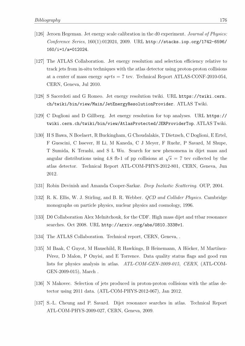
Bibliography 176
[126] Jeroen Hegeman. Jet energy scale calibration in the d0 experiment. Journal of Physics:
Conference Series, 160(1):012024, 2009. URL http://stacks.iop.org/1742-6596/
160/i=1/a=012024.
[127] The ATLAS Collaboration. Jet energy resolution and selection efficiency relative to
track jets from in-situ techniques with the atlas detector using proton-proton collisions
at a center of mass energy sqrts = 7 tev. Technical Report ATLAS-CONF-2010-054,
CERN, Geneva, Jul 2010.
[128] S Sacerdoti and G Romeo. Jet energy resolution twiki. URL https://twiki.cern.
ch/twiki/bin/view/Main/JetEnergyResolutionProvider. ATLAS Twiki.
[129] C Doglioni and D Gillberg. Jet energy resolution for top analyses. URL https://
twiki.cern.ch/twiki/bin/view/AtlasProtected/JERProviderTop. ATLAS Twiki.
[130] H S Bawa, N Boelaert, R Buckingham, G Choudalakis, T Dietzsch, C Doglioni, E Ertel,
F Guescini, C Issever, H Li, M Kaneda, C J Meyer, F Ruehr, P Savard, M Shupe,
T Sumida, K Terashi, and S L Wu. Search for new phenomena in dijet mass and
angular distributions using 4.8 fb-1 of pp collisions at√s = 7 tev collected by the
atlas detector. Technical Report ATL-COM-PHYS-2012-801, CERN, Geneva, Jun
2012.
[131] Robin Devinish and Amanda Cooper-Sarkar. Deep Inelastic Scattering. OUP, 2004.
[132] R. K. Ellis, W. J. Stirling, and B. R. Webber. QCD and Collider Physics. Cambridge
monographs on particle physics, nuclear physics and cosmology, 1996.
[133] D0 Collaboration Alex Melnitchouk, for the CDF. High mass dijet and ttbar resonance
searches. Oct 2008. URL http://arxiv.org/abs/0810.3338v1.
[134] The ATLAS Collaboration. Technical report, CERN, Geneva, .
[135] M Baak, C Guyot, M Hauschild, R Hawkings, B Heinemann, A Hocker, M Martınez-
Perez, D Malon, P Onyisi, and E Torrence. Data quality status flags and good run
lists for physics analysis in atlas. ATL-COM-GEN-2009-015, CERN, (ATL-COM-
GEN-2009-015), March .
[136] N Makovec. Selection of jets produced in proton-proton collisions with the atlas de-
tector using 2011 data. (ATL-COM-PHYS-2012-067), Jan 2012.
[137] S.-L. Cheung and P. Savard. Dijet resonance searches in atlas. Technical Report
ATL-COM-PHYS-2009-027, CERN, Geneva, 2009.
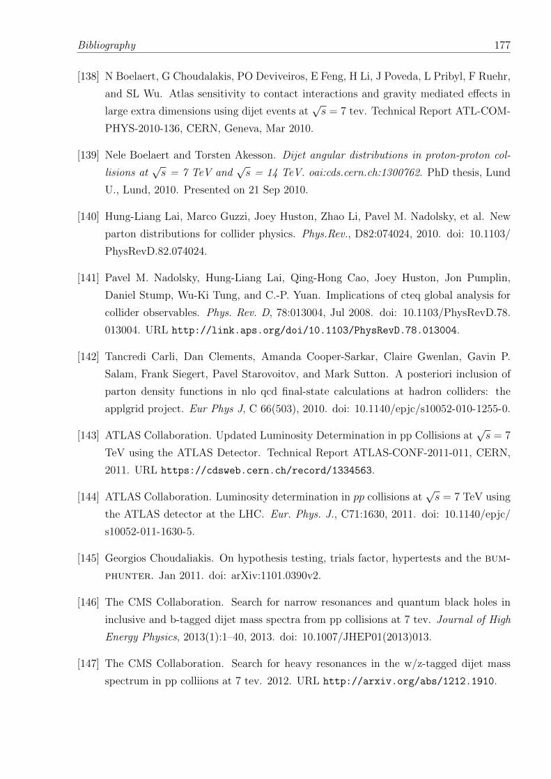
Bibliography 177
[138] N Boelaert, G Choudalakis, PO Deviveiros, E Feng, H Li, J Poveda, L Pribyl, F Ruehr,
and SL Wu. Atlas sensitivity to contact interactions and gravity mediated effects in
large extra dimensions using dijet events at√s = 7 tev. Technical Report ATL-COM-
PHYS-2010-136, CERN, Geneva, Mar 2010.
[139] Nele Boelaert and Torsten Akesson. Dijet angular distributions in proton-proton col-
lisions at√s = 7 TeV and
√s = 14 TeV. oai:cds.cern.ch:1300762. PhD thesis, Lund
U., Lund, 2010. Presented on 21 Sep 2010.
[140] Hung-Liang Lai, Marco Guzzi, Joey Huston, Zhao Li, Pavel M. Nadolsky, et al. New
parton distributions for collider physics. Phys.Rev., D82:074024, 2010. doi: 10.1103/
PhysRevD.82.074024.
[141] Pavel M. Nadolsky, Hung-Liang Lai, Qing-Hong Cao, Joey Huston, Jon Pumplin,
Daniel Stump, Wu-Ki Tung, and C.-P. Yuan. Implications of cteq global analysis for
collider observables. Phys. Rev. D, 78:013004, Jul 2008. doi: 10.1103/PhysRevD.78.
013004. URL http://link.aps.org/doi/10.1103/PhysRevD.78.013004.
[142] Tancredi Carli, Dan Clements, Amanda Cooper-Sarkar, Claire Gwenlan, Gavin P.
Salam, Frank Siegert, Pavel Starovoitov, and Mark Sutton. A posteriori inclusion of
parton density functions in nlo qcd final-state calculations at hadron colliders: the
applgrid project. Eur Phys J, C 66(503), 2010. doi: 10.1140/epjc/s10052-010-1255-0.
[143] ATLAS Collaboration. Updated Luminosity Determination in pp Collisions at√s = 7
TeV using the ATLAS Detector. Technical Report ATLAS-CONF-2011-011, CERN,
2011. URL https://cdsweb.cern.ch/record/1334563.
[144] ATLAS Collaboration. Luminosity determination in pp collisions at√s = 7 TeV using
the ATLAS detector at the LHC. Eur. Phys. J., C71:1630, 2011. doi: 10.1140/epjc/
s10052-011-1630-5.
[145] Georgios Choudaliakis. On hypothesis testing, trials factor, hypertests and the bum-
phunter. Jan 2011. doi: arXiv:1101.0390v2.
[146] The CMS Collaboration. Search for narrow resonances and quantum black holes in
inclusive and b-tagged dijet mass spectra from pp collisions at 7 tev. Journal of High
Energy Physics, 2013(1):1–40, 2013. doi: 10.1007/JHEP01(2013)013.
[147] The CMS Collaboration. Search for heavy resonances in the w/z-tagged dijet mass
spectrum in pp colliions at 7 tev. 2012. URL http://arxiv.org/abs/1212.1910.
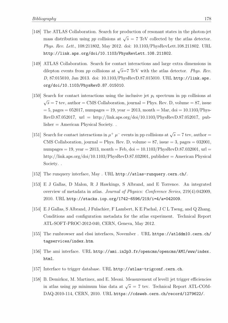
Bibliography 178
[148] The ATLAS Collaboration. Search for production of resonant states in the photon-jet
mass distribution using pp collisions at√s = 7 TeV collected by the atlas detector.
Phys. Rev. Lett., 108:211802, May 2012. doi: 10.1103/PhysRevLett.108.211802. URL
http://link.aps.org/doi/10.1103/PhysRevLett.108.211802.
[149] ATLAS Collaboration. Search for contact interactions and large extra dimensions in
dilepton events from pp collisions at√s=7 TeV with the atlas detector. Phys. Rev.
D, 87:015010, Jan 2013. doi: 10.1103/PhysRevD.87.015010. URL http://link.aps.
org/doi/10.1103/PhysRevD.87.015010.
[150] Search for contact interactions using the inclusive jet pt spectrum in pp collisions at√s = 7 tev, author = CMS Collaboration, journal = Phys. Rev. D, volume = 87, issue
= 5, pages = 052017, numpages = 19, year = 2013, month = Mar, doi = 10.1103/Phys-
RevD.87.052017, url = http://link.aps.org/doi/10.1103/PhysRevD.87.052017, pub-
lisher = American Physical Society. .
[151] Search for contact interactions in µ+ µ− events in pp collisions at√s = 7 tev, author =
CMS Collaboration, journal = Phys. Rev. D, volume = 87, issue = 3, pages = 032001,
numpages = 19, year = 2013, month = Feb, doi = 10.1103/PhysRevD.87.032001, url =
http://link.aps.org/doi/10.1103/PhysRevD.87.032001, publisher = American Physical
Society. .
[152] The runquery interface, May . URL http://atlas-runquery.cern.ch/.
[153] E J Gallas, D Malon, R J Hawkings, S Albrand, and E Torrence. An integrated
overview of metadata in atlas. Journal of Physics: Conference Series, 219(4):042009,
2010. URL http://stacks.iop.org/1742-6596/219/i=4/a=042009.
[154] E J Gallas, S Albrand, J Fulachier, F Lambert, K E Pachal, J C L Tseng, and Q Zhang.
Conditions and configuration metadata for the atlas experiment. Technical Report
ATL-SOFT-PROC-2012-040, CERN, Geneva, May 2012.
[155] The runbrowser and elssi interfaces, November . URL https://atlddm10.cern.ch/
tagservices/index.htm.
[156] The ami interface. URL http://ami.in2p3.fr/opencms/opencms/AMI/www/index.
html.
[157] Interface to trigger database. URL http://atlas-trigconf.cern.ch.
[158] B. Demirkoz, M. Martinez, and E. Meoni. Measurement of level1 jet trigger efficiencies
in atlas using pp minimum bias data at√s = 7 tev. Technical Report ATL-COM-
DAQ-2010-114, CERN, 2010. URL https://cdsweb.cern.ch/record/1279622/.

Bibliography 179
[159] The ATLAS Collaboration. Measurement of inclusive jet and dijet production in pp
collisions at√s=7 TeV using the atlas detector. Phys. Rev. D, 86:014022, Jul 2012. doi:
10.1103/PhysRevD.86.014022. URL http://link.aps.org/doi/10.1103/PhysRevD.
86.014022.