Embed Size (px)
Citation preview

JHEP06(2014)046
Published for SISSA by Springer
Received: August 9, 2013
Revised: February 26, 2014
Accepted: May 16, 2014
Published: June 9, 2014
Searching for Fermi surfaces in super-QED
Aleksey Cherman,a Saso Grozdanovb and Edward Hardyb
aFine Theoretical Physics Institute, Department of Physics, University of Minnesota,
116 Church St SE, Minneapolis MN 55455 U.S.A.bRudolf Peierls Centre for Theoretical Physics, University of Oxford,
1 Keble Road, Oxford OX1 3NP, U.K.
E-mail: [email protected], [email protected],
Abstract: The exploration of strongly-interacting finite-density states of matter has been
a major recent application of gauge-gravity duality. When the theories involved have a
known Lagrangian description, they are typically deformations of large N supersymmetric
gauge theories, which are unusual from a condensed-matter point of view. In order to
better interpret the strong-coupling results from holography, an understanding of the weak-
coupling behavior of such gauge theories would be useful for comparison. We take a first
step in this direction by studying several simple supersymmetric and non-supersymmetric
toy model gauge theories at zero temperature. Our supersymmetric examples are N = 1
super-QED and N = 2 super-QED, with finite densities of electron number and R-charge
respectively. Despite the fact that fermionic fields couple to the chemical potentials we
introduce, the structure of the interaction terms is such that in both of the supersymmetric
cases the fermions do not develop a Fermi surface. One might suspect that all of the charge
in such theories would be stored in the scalar condensates, but we show that this is not
necessarily the case by giving an example of a theory without a Fermi surface where the
fermions still manage to contribute to the charge density.
Keywords: Supersymmetric gauge theory, Holography and condensed matter physics
(AdS/CMT)
ArXiv ePrint: 1308.0335
Open Access, c© The Authors.
Article funded by SCOAP3.doi:10.1007/JHEP06(2014)046

JHEP06(2014)046
Contents
1 Introduction 1
2 What should we expect? 5
2.1 Summary of expectations 9
3 N = 1 sQED at finite electron number density 10
3.1 Scalar ground state 10
3.2 Search for a Fermi surface 13
3.3 Non-supersymmetric cousin of N = 1 sQED 15
4 Softly broken N = 2 sQED at finite electron number density 17
4.1 Scalar ground state 17
4.2 Search for a Fermi surface 19
4.3 Non-supersymmetric cousin of N = 2 sQED 21
5 N = 2 sQED with a finite R-charge density 23
5.1 Scalar ground state 24
5.2 Search for a Fermi surface 25
6 Fermion charge density without a Fermi surface 26
7 Discussion 32
1 Introduction
Understanding the behavior of quantum matter at finite temperature T and density µ is a
major challenge in many areas of physics, ranging from traditional condensed matter topics
to quark-gluon plasmas as explored at RHIC and the LHC, to the behavior of super-dense
QCD matter in the cores of neutron stars. Developing such an understanding is especially
difficult when the systems are strongly coupled and traditional perturbative techniques
are not useful. One powerful non-perturbative technique which has attracted a great deal
of attention in recent years is gauge-gravity duality [1], which maps questions about some
special strongly-coupled field theories to questions about weakly-coupled theories of gravity,
which are much easier to work with. (For reviews, see e.g. [2, 3], and especially [4], which
has a focus on Fermi surfaces.) This has led to many interesting results for the study of
finite-density quantum matter, but also a number of puzzles, such as the fate of Fermi
surfaces in the strongly-coupled systems which have gravity duals.
– 1 –

JHEP06(2014)046
The ability to do controlled calculations on the gravity side of the duality comes with
several conditions and costs. To justify treating the gravity side of the duality classically,
which is in general the only tractable limit, one needs the field theory to be (1) strongly
coupled, typically in the sense of having a tunable ’t Hooft coupling which is taken to be
large and (2) to be in some kind of large N limit. Indeed, in all of the cases where the
dual field theory Lagrangian is explicitly known, the field theory is a non-Abelian gauge
theory, and the parameter N is associated with the rank of the gauge group.1 Finally, the
class of theories which have strong-coupling limits and a large N limit is clearly rather
special,2 and in all of the cases where the dual field theory Lagrangians are known, they
are supersymmetric gauge theories or deformations thereof, see e.g. [1, 5–8] for some pro-
totypical examples.
These considerations make it difficult to tell a priori which of the many interesting
results gauge-gravity duality has yielded are due to strong coupling, large N , the special
nature of the field content and interactions in the theories which have gravity duals, or
some combination of these. In this sense, gauge-gravity duality is essentially a black box,
since it is only tractable in a limit where the field theory description is fundamentally
difficult to work with. Moreover, while the duality has yielded many striking results, it
has also produced many mysteries, such as the fate of Fermi surfaces at strong coupling,
explored in e.g. [9–27]. The ‘microscopic’ field content of the theories with gravity duals
generally includes gauge bosons, fermions, and scalars, with the number of degrees of
freedom for all of these scaling as O(N2) in the 4D field theory examples. In these theories
chemical potentials for conserved charges usually couple to both the scalars and fermions
at the microscopic level. Hence if intuition derived from studies of weakly-coupled non-
supersymmetric theories were to be boldly applied to the strong coupling limit of the kind
of theories which have gravity duals, then one might have expected that Fermi surfaces
would be ubiquitous in systems with gravity duals.
However, while Fermi surfaces have shown up in some examples of gauge-gravity dual-
ity, they do not seem to be at all ubiquitous. Signs of Fermi surfaces for the O(N2) degrees
of freedom have recently shown up in e.g. [14] in correlation functions of fermionic operators
in electron star geometries [13, 28], and in some top-down calculations in [26, 27] for 4D the-
ories. But in other examples Fermi surfaces appear to be absent [15, 16]. Meanwhile, Fermi
surfaces have been observed in fermionic correlators of O(N0) densities of probe fermions in
work initiated in [9, 10]. To make the situation more complicated, naively — that is, based
on expectations from weak-coupling studies of systems familiar from condensed matter —
Fermi surfaces should have an imprint on bosonic correlation functions as well, showing
up as e.g. momentum-space singularities in density-density correlation functions leading to
Friedel oscillations. Indeed, in holography one only has access to gauge-invariant observ-
ables, while Fermi surfaces for the quarks in a gauge theory would not be gauge-invariant.
So such Fermi surfaces might be ‘hidden’ [19] in the gravity duals, and hence singularities
1Finding such a large parameter in the known phenomenologically-relevant examples is a challenge,
especially in the examples from condensed matter.2For instance, large N QCD is not such a theory, since its ’t Hooft coupling runs, and is thus not a
tunable control parameter.
– 2 –
JHEP06(2014)046
in gauge-invariant charge density correlation functions may seem to be especially promising
places to look for traces of Fermi surface physics. But such density-correlator signatures
of underlying Fermi surfaces have not been seen in many holographic systems.3
These considerations motivate our belief that to better understand the results of
gauge/gravity duality calculations, it would be very useful to reexamine some observables
for which strong coupling results from holography are available at weak coupling using
conventional field-theory techniques, where one can see all of the moving pieces. In partic-
ular, one would have direct access to any ‘hidden’ Fermi surfaces, since at weak coupling it
makes sense to work in a gauge-fixed formalism. We will focus on D = 3 + 1 dimensional
theories for simplicity, and confine our attention to the T = 0 limit. Our metric signature
convention is (+−−−).
An example of the kind of theory one might want to study at weak coupling is N = 4
super-Yang-Mills theory with a chemical potential for R-charge, where the number of
charged degrees of freedom scales as N2, originally studied in [31–34]. Another exam-
ple, where the number of charged degrees of freedom scales as N1, is the N = 2 gauge
theory dual to Nf D7 branes intersecting Nc D3 branes in the ‘quenched’ Nf/Nc 1
approximation [5]. The study of this latter flavored N = 2 system at finite quark number
density was initiated in [35]. Calculations using the gravity side of the duality predict
unusual thermodynamical features for this theory which are not known to arise from any
weakly-coupled theory, with e.g. a specific heat with the temperature scaling cV ∼ T 6 [36],
in contrast to what one might expect from a Fermi liquid where cV ∼ T . Moreover, [36]
found a gapless quasiparticle mode in the system which was argued to be Landau’s zero
sound mode (see also [37–41] for some further exploration of this identification). But the cVscaling shows that the system is clearly a non-Fermi liquid, and to the extent that the dual
field theory is a gauge theory with gapless gauge interactions, a zero sound mode would
be surprising, at least at weak coupling, as we discuss further in section 2. What is the
origin of the curious thermodynamic properties of this system and what is the true identity
of the quasiparticles modes? It is possible that the puzzling thermodynamics is driven by
some intrinsically strongly-coupled physics, or — as explored recently in e.g. [41–43] — the
calculations of [36] were done in some metastable vacuum. Another possibility, which can
be explored using weak-coupling techniques, is that at least some of these properties are a
consequence of the unusual field content and interactions of the field theory.
However, as with the other theories with known field theory Lagrangians and gravity
duals, the N = 4 super-Yang-Mills field theory examined in [1] is quite complicated, as are
its cousins discussed in the many follow-up works, and we will not address field theories
with gravity duals directly in this work. Instead, as a first step we will study a few simpler
toy-model supersymmetric gauge theories. Specifically, we will explore the behavior of
N = 1 super-QED (sQED) and N = 2 sQED in the presence of chemical potentials at
zero temperature. Even these simple toy models show some curious features, since from a
condensed-matter point of view they have unusual field content and interactions, with the
3In [24] it is observed that density-density correlation functions in theories with dual Lifshitz geome-
tries [29, 30] with z =∞ have momentum-space singularities which suggest the presence of a Fermi surface,
but z <∞ examples do not.
– 3 –

JHEP06(2014)046
chemical potential coupling to both scalar fields and fermions, which are in turn coupled
to each other by the demands of supersymmetry.
Perhaps the simplest questions one can ask about such systems concern the nature
of their ground states. Do the bosons condense, and do the fermions develop a Fermi
surface?4 It seems natural to expect weakly-coupled scalars to condense at T = 0 in
response to a chemical potential, and we find that this is indeed what happens in our
examples. One might expect Fermi surfaces to be a generic consequence of turning on
chemical potentials that couple to weakly-interacting fermions based on a naive application
of the standard Landau Fermi liquid picture, and intuitions derived from thinking about
non-supersymmetric electron plasmas. But we find that dense plasmas based on N = 1
andN = 2 sQED fail to be Fermi liquids in a fairly dramatic way, already at weak coupling.
While the chemical potential couples to the fermions in all of our examples, it does not
lead to a Fermi surface in most of them. This suggests another possible reason for the
mysterious cases of missing Fermi surfaces encountered in holographic studies, aside from
strong coupling.
This paper is organized as follows. First, in section 2, we give an overview of our toy
models, explain their unusual features from a condensed-matter perspective, and discuss
what one might expect for their behavior at finite density. The impatient reader may
wish to look only at the summary in section 2.1. In section 3, we explore N = 1 sQED
at finite electron number density. Then in section 4 we discuss N = 2 sQED with a
finite electron number density, where we are forced to introduce some soft SUSY-breaking
terms to stabilize the scalar sector. Next, in section 5 we look at N = 2 sQED with a
finite R-charge density. Algebraically, the N = 2 R-charged theory and its SUSY-broken
cousins are our cleanest examples, and we evaluate the fermion contribution to the charge
density for some examples in this class of theories. The somewhat surprising result of this
investigation is described in section 6. Finally, in section 7 we summarize our findings and
sketch some of the many possible directions for future work.
We also make a brief comment on the existing literature on supersymmetric gauge
theories at finite density using field-theoretic techniques. The works closest in spirit to
ours that we are aware of are [44, 45] and [18]. Ref. [44] studied N = 4 SYM theory with
R-charge chemical potentials compactified on a 3-sphere, with a focus mostly on the high-T
limit, while [45] studied the finite-T properties of N = 2 super-Yang-Mills (SYM) theory.
Ref. [19] studied physics related to Fermi surfaces in non-supersymmetric theories inspired
by 4D N = 4 SYM, among other examples, but with their choice of models they did not run
into many of the issues we deal with here. We also note the important work [46] exploring
the interplay between Luttinger’s theorem, Fermi surfaces, and Bose-Einstein condensation
in the context of cold atomic gases.
Also, the study of super-QCD at finite quark-number was initiated in [47] for N = 1
supersymmetry and in [48] for N = 2 supersymmetry, with an aim of understanding color
superconductivity in a supersymmetric context. However, the issue of the existence of
4We are very grateful to David Tong for an early discussion challenging our naive assumption that Fermi
surfaces are inevitable at weak coupling.
– 4 –

JHEP06(2014)046
Fermi surfaces in supersymmetric gauge theories at finite density was not examined in
these papers. Finally, the interesting recent works [49, 50] constructed a supersymmetric
version of ‘BCS theory’, without dynamical gauge fields, and engineered things such that
there is no scalar condensation but there are Fermi surfaces.
2 What should we expect?
The standard example of a finite-density relativistic system involving fermions and gauge
fields is a QED plasma, which we now briefly describe before considering supersymmetric
theories. We do this because much of our intuition for what to expect for finite-density
physics is based on experience with this non-supersymmetric system.
The Lagrangian describing an electron plasma is just that of QED, involving the elec-
tron field ψ and the photon gauge field Aµ, and is very simple:
LN= 0 = −1
4FµνF
µν + ψ (i /D −m)ψ +AµJµ, (2.1)
where Dµ = ∂µ − iµδµ0 − igAµ, g is the gauge coupling, µ is a chemical potential which
couples to the charge of the electrons, and Jµ encodes the effects of other matter which
provides a neutralizing background, such as some ions.
The requirement of having a neutralizing background is essential. While the addition
of the chemical potential term is a gauge-invariant deformation of the theory, it couples to a
gauged charge. If one wants a finite density of matter in the vacuum in the infinite-volume
limit, with a finite free energy density, then any negative charge density carried by the
electrons must be compensated by a positive charge density carried by the ions. Otherwise
one would pay an infrared-divergent energy cost for having long-range electric fields. This
is a textbook observation for QED plasmas [51], and is also true for non-Abelian gauge
theories like QCD at high densities.5 As is explained in e.g. section 2 in [53], neutrality
must be imposed even if the gauged charge is spontaneously broken, which will be relevant
for our discussion of sQED. Otherwise a finite size chunk of the degenerate matter would
have electric fields outside of it which grow in strength with its size, again causing problems
with the infinite-volume limit.
Before beginning a discussion of supersymmetric plasmas, and exploring to what extent
they can be thought of as Fermi liquids, it is important to note that a standard dense low-
temperature electron gas described by eq. (2.1) is already not a Fermi liquid. The issue is
the long range of the electromagnetic interactions, and the subtle nature of screening due
to the degenerate electrons. While Coulomb photons pick up a screening mass in the static
(zero-frequency) limit due to medium effects, the transverse (‘magnetic’) photons do not
get a static screening mass so long as the photons do not become Higgsed. Consequently,
the magnetic photons continue to mediate long-range interactions, and this drives the
breakdown of Fermi liquid theory [56–59]. This leads to subtle effects such as a non-Fermi-
liquid scaling of the specific heat with temperature, cv ∼ T lnT , among others. At a
more pedestrian level, the non-trivial momentum and energy dependence of the Coulomb
5For some seminal papers exploring this issue e.g. see [52–54], for a review see [55].
– 5 –

JHEP06(2014)046
screening effects in an electron plasma are such that the residual Coulomb interaction
obliterates the would-be gapless Fermi zero-sound mode present in Fermi liquids, turning
it into the gapped plasmon mode of the dense electron gas as explained in e.g. chapter 16
of the textbook [51].
Given these results for non-supersymmetric gauge theories at finite density, we clearly
cannot assume that the N = 1 and N = 2 sQED plasmas should be Fermi liquids.
Nevertheless, while non-supersymmetric degenerate plasmas are not Fermi liquids, the
fermions populating the plasma still have a Fermi surface, at least before considering the
standard sort of pairing (superconducting) instabilities which can lead to its breakdown.
This remains true6 even in more exotic non-supersymmetric systems, such as degenerate
quark matter, and generalizations of eq. (2.1) to include condensed dynamical scalar fields
in Jµ [60–63], or some types of Yukawa interactions [64]. As we will see, however, even the
very existence of a Fermi surface cannot be taken for granted in the supersymmetric case.
For a final observation about non-supersymmetric plasmas, we note that having g 1
is necessary but not sufficient for a QED plasma to be weakly coupled. The reason is
that Coulomb interactions are, in a sense, strong at low energies, and tend to lead to
the formation of bound states — atoms — if the interaction energy dominates over the
characteristic momenta of the electrons and ions. Indeed, if we define l ≡ [3/(4πn)]1/3 as
the inter-electron ‘spacing’ and denote the Bohr radius by a0 ≡ 1/(αm), then it is well-
known that in an electron gas the physical expansion parameter is rs ≡ l/a0, rather than
α ≡ g2/4π, and one must have rs 1 for calculability. We expect that our results in
the supersymmetric examples below will be reliable in a similar high density limit, but it
will be important to verify this in future work by doing higher-order calculations. For this
work, we simply assume that our number densities are large enough that we do not have to
worry about the formation of supersymmetric atoms, which were studied recently in [65–
67]. In the terminology often used in the AdS/CMT literature, our focus on high density
fully ionized plasmas means that we work in the ‘fractionalized’ regime of super QED, as
opposed to the low-density atomic gas regime, which could be thought of as ‘confined’.
We now turn to a discussion of the subtleties particular to supersymmetric plasmas.
To keep the discussion streamlined, we use N = 1 sQED as our example. The action of
N = 1 sQED is significantly more complicated than that of QED. In addition to ψ and
Aµ, supersymmetry requires the addition of selectron fields φ+, φ−, as well as the gaugino
λ, along with interaction terms amongst all of these mandated by the supersymmetrization
of the gauge interaction. The resulting action is
LN= 1 = − 1
4FµνF
µν +1
2λi/∂λ
+ ψ(i /D− −m
)ψ +
∣∣D−µ φ−∣∣2 +∣∣D+
µ φ+
∣∣2 − |mφ−|2 − |mφ+|2
6Since electron and quark fields are not gauge invariant, the notion of a Fermi surface is easiest to
discuss in a gauge-fixed setting, and understanding its effects in gauge-invariant language requires more
work. Fortunately, at weak coupling, where our attention will be confined, the use of such gauge-fixed
notions will be very useful, as it is in e.g. the standard discussions of gauge symmetry ‘breaking’ in the
Standard Model’s Higgs mechanism.
– 6 –

JHEP06(2014)046
+√
2ig(φ†+ψP−λ− φ
†−λP−ψ − φ+λP+ψ + φ−ψP+λ
)− g2
2
(|φ+|2 − |φ−|2
)2
+ Ions, (2.2)
where λ is a Majorana fermion, P± = 12(1± γ5), φ± are complex scalar fields,
D±µ = ∂µ ± iµδµ0 ± igAµ (2.3)
and the +Ions term encodes couplings to neutralizing ‘ion’ fields. We assume the ion sector
is supersymmetric as well, and defer writing out the relevant contributions to the action for
now. The physical motivation for assuming that the ion sector is supersymmetric is that
the theories we are really interested in — the ones with gravity duals — usually do not
include dynamical non-supersymmetric sectors. The action describing N = 2 matter at
finite density is even more complex, and we do not write it out here; the general comments
about N = 1 sQED below also apply to N = 2 sQED.
Before launching a search for Fermi surfaces in N = 1 sQED, and then N = 2 sQED,
we should emphasize a few features of eq. (2.2) which make the analysis tricky. First,
note that before considering the ‘ions’, there is only one continuous symmetry in eq. (2.2),
under which the fields have the transformation properties ψ → e−iαψ, φ+ → eiαφ+, φ− →e−iαφ−, Aµ → Aµ, λ→ λ. So there are no separate fermion number or scalar number sym-
metries, in a striking contrast to familiar non-supersymmetric theories, even ones studied
in [46]. The fields are tied together by the Yukawa interactions in such a way that only
a single U(1) remains. Second, we observe that as usual, the chemical potential enters
the Lagrangian as the time component of a background gauge field. So both the selectron
and the electron fields directly experience the chemical potential. We note that in this
situation, one should interpret any expectations based on Luttinger’s theorem [68] or the
theory of ‘compressible quantum matter’ [18] with care, since the assumptions underly-
ing these frameworks do not apply in general to the systems we consider once the scalar
fields condense.
The issue we explore in this work concerns the response of the selectrons and electrons
to the chemical potential. Let us start by considering the behavior of the scalar fields of
N = 1 sQED. The scalar effective potential Veff is the sum of the classical potential
V(0)
eff = (|m|2 − µ2)(|φ+|2 + |φ−|2) +g2
2(|φ+|2 − |φ−|2)2 (2.4)
plus quantum corrections. Interactions with the electrons and photons will contribute
new terms to the bosonic effective potential starting at one loop level. But so long as
the theory is weakly coupled, and the classical potential is non-vanishing, the selectron
ground state should be determined by V(0)
eff , since quantum corrections to V(0)
eff should be
comparatively small.
From the form of V(0)
eff , one might think that once µ > m, the scalars should condense,
breaking the U(1) gauge symmetry and making the system a superconductor. Moreover,
since the masses of the electrons and selectrons are fixed to be identical due to supersym-
metry, the fermions should naively start populating a Fermi surfaces at the same time that
the scalars start condensing.
– 7 –

JHEP06(2014)046
But there is an immediate subtlety we must deal with: supersymmetric gauge theories
typically have moduli spaces protected by supersymmetry at µ = 0. In the current context,
the moduli space for m = 0, µ = 0 is isomorphic to C, and is parametrized by the value of
φ+ = φ−. For any set of vacuum expectation values for the selectrons satisfying φ+ = φ−,
the potential energy vanishes. But as soon as we make µ > m, V(0)
eff develops a runaway
direction along φ+ = φ−. That is, the effective potential becomes unbounded from below,
and the theory as defined in eq. (2.2) does not make sense for µ > m.7
This should not be especially surprising. For a system comprised of weakly-interacting
bosonic particles to be stable at finite chemical potential, the bosons must have sufficiently
repulsive interactions. If the interactions of the bosons were attractive, then the system
would be unstable against a collapse towards arbitrarily high densities, and there would
not be any equilibrium finite-density ground state. This is precisely the issue that one faces
in N = 1 sQED, where supersymmetry demands the presence of an attractive interaction
between the positive and negative selectrons −g2
2 |φ+|2|φ−|2. The arguments above imply
that this issue indeed causes an instability which is unavoidable without deforming the
theory in some way.
Fortunately, in N = 1 sQED, it is possible to dodge this problem by turning on a
Fayet-Iliopulous term, which does not explicitly break the supersymmetry of the action,
and has the effect of modifying the potential to
V(0)
eff = (|m|2 − µ2)(|φ+|2 + |φ−|2) +g2
2(|φ+|2 − |φ−|2 − ξ2)2, (2.5)
where ξ2 can be either positive or negative, and has mass dimension two. At µ = 0, this
lifts the moduli space, and indeed supersymmetry becomes spontaneously broken for ξ > 0
so long as m 6= 0. With ξ turned on, we will argue that the selectrons of the theory have
a stable non-trivial ground state for µ in a certain range. Hence the naive expectation
that the U(1) gauge symmetry is broken at finite density is borne out, and the system is a
superconductor.
One might have hoped that so long as g 1, and the system is weakly coupled, the
response of the electrons to the chemical potential should resemble that of the free limit
g = 0. This is true in a QED plasma. However, one should not expect it to be true in
general for supersymmetric plasmas, as we now explain.
First, it is clear from the structure of the Yukawa terms in eq. (2.2), which include
terms of the form
g φ†+ψP−λ, (2.6)
that turning on scalar VEVs leads to mixing between the electron and gaugino fields, and
this makes it difficult to guess what the fermionic fields will do in response to a chemical
potential for the electrons just by looking at eq. (2.2). The way to deal with this is
7If both a finite µ and finite temperature T are turned on, things may be different, since the finite
temperature breaks supersymmetry, and should help lift the moduli space at µ = 0. For an interesting
recent exploration of finite-T physics in a supersymmetric gauge theory using field-theoretic techniques,
see [45].
– 8 –

JHEP06(2014)046
obvious in principle, since one just has to rotate to an eigenbasis where the kinetic terms
for the fermions become diagonal in the in-medium ‘flavors’, but in practice actually doing
such a rotation can be algebraically involved. Since the coefficient of the mixing term is
proportional to g, however, one might have hoped that when g 1, the mixing would be
small, and the response of the fermions to a chemical potential would be close to that of
the g = 0 system.
To see why this expectation is too naive, note that the coefficient of the Yukawa terms
is forced to be the gauge coupling g by supersymmetry. But the coefficient controlling
the strength of the self-interaction of the selectrons in eq. (2.5) is g2, which is also fixed
by supersymmetry. So unlike in a non-supersymmetric system, here the strengths of the
Yukawa interactions and the selectron self-interactions cannot be tuned independently. In
particular, given the form of the selectron potential it is obvious that a non-zero selectron
VEV 〈φ〉 must scale as
〈φ〉 ∼ 1
g. (2.7)
So since the size of the electron-gaugino mixing terms is controlled by g〈φ〉, we see that
the fermion mixing will be essentially independent of g. The mixing alters the dispersion
relations of the fermion fields at the quadratic level, and so we cannot assume that the
response of the electrons to a chemical potential at g = 0, which involves the formation
of a Fermi surface, will necessarily persist to any g > 0, no matter how small. This
observation is generic, and applies to essentially any supersymmetric gauge theory in which
one turns on a chemical potential for selectrons or squarks which can also cause selectron
or squark condensation.
2.1 Summary of expectations
For the reasons discussed above, we expect that:
• The chemical potentials we will consider couple to both fermions and scalars, and so
long as the theory is supersymmetric we expect the scalars to condense at the same
time as the fermions begin to feel the chemical potential. This means the U(1) gauge
symmetry will be broken, and the supersymmetric plasmas will be superconductors.
• It is essential to take into account the electric neutrality constraint. In a related
context, this was also emphasized in [18].
• We assume that the densities are large enough that we do not have to worry about
the formation of supersymmetric atoms, so that we deal with a completely ionized
plasma. This means we are focusing on the fractionalized regime of the plasma, as
opposed to the low-density atomic gas confined regime.
• Achieving a stable finite-density ground state may be tricky due to possible run-away
directions in the scalar potential due to supersymmetry.
– 9 –

JHEP06(2014)046
• We should not expect the behavior of the fermions to be close to that of a conventional
free system once there is scalar condensation, because of the structure of the Yukawa
interactions and the scalar self-interactions dictated by supersymmetry.
• If the scalars condense, the fact that the U(1) electron number symmetry is shared
between the scalars and the fermions means that the resulting quantum liquids will
not be ‘compressible quantum matter’ as it is defined in [19]. Moreover, the assump-
tions of Luttinger’s theorem [68], which ties the charge density carried by a fermionic
system to the volume of the Fermi surface, will not apply to such a liquid. So we
should not expect the existence of Fermi surfaces to be automatic for finite-density
supersymmetric QED.
With these observations in mind, we turn to a more detailed examination of these
issues in our N = 1 and N = 2 sQED toy models.
3 N = 1 sQED at finite electron number density
3.1 Scalar ground state
We now write down the complete N = 1 action we will consider. We include two chiral
superfields Φ+ and Φ− which supply the matter fields for the ‘electron’ sector: the electron
Dirac spinor field ψ, as well the bosonic selectrons φ+, φ−. We also include two other chiral
superfields Q+ and Q−, which supply the matter fields for the ‘ion’ sector: the ion Dirac
spinor field η, as well as the bosonic sion fields q+, q−. We consider a superpotential of the
simplest possible form
W = m(Φ+Φ− +Q+Q−), (3.1)
so that the ions and the electrons have the same mass m. The tree-level Kahler potential is
K = Φ†+eV Φ+ + Φ†−e
−V Φ− +Q†+eVQ+ +Q†−e
−VQ−, (3.2)
and V is the vector superfield, which includes the photon and photino fields Aµ, λ. We
also allow a Fayet-Iliopoulos term
Lξ = −ξ2
∫d4θV. (3.3)
The Lagrangian of the version of N = 1 SQED that we will consider is thus
LN= 1 =
(1
4g2
∫d2θW 2 + h.c.
)+
∫d4θK +
(∫d2θW + h.c.
)+ Lξ, (3.4)
and Wα is the photon field strength chiral super field.
The matter sector has two obvious U(1) symmetries, U(1)e and U(1)i, which act on
the component fields as shown in table 1. The diagonal U(1)e × U(1)i symmetry (acting
as ψ → e−iαψ, η → e−iαη, and so on) is gauged, and we will refer to the gauged charge as
the ‘electric’ charge.
– 10 –

JHEP06(2014)046
Transformation Properties in N = 1 sQED
Fields: ψ φ+ φ− λ η q+ q−
U(1)e e−iαψ e+iαφ+ eiαφ− λ η q+ q−
U(1)i ψ φ+ φ− λ e−iαη e+iαq+ e−iαq−
Table 1. Matter field transformation properties under the U(1)e and U(1)i symmetries.
We want to have a net density of electron-sector fields — electrons, selectrons, or
both — in the ground state. To do this we turn on a chemical potential µe for the U(1)esymmetry, which appears in the action as the time component of a background gauge field
coupling only to U(1)e charge. At the same time, we wish to maintain charge neutrality.
To do this, we also turn on a chemical potential µi for the conserved charge associated with
the ion U(1)i symmetry. Then the µe chemical potential can be viewed as the parameter
controlling the matter density of the system, while µi is an auxiliary parameter determined
by the requirement of charge neutrality.
It turns out that setting µ ≡ µe = −µi will be sufficient to maintain charge neutrality.
Heuristically, turning on µ > 0 gives an equal energetic subsidy to the particles created by
the field operators ψ, φ−, φ+ and the antiparticles created by η, q−, q+. Since these two
sets of particles and antiparticles have the same masses but opposite electric charges, this
will create a ground state which is electrically neutral. To see this in a more quantitative
way, recall that we can read off the expression for the charge density from the part of the
action which is linear in A0:
gA0Q ∈ L, (3.5)
since A0 is, by definition, the source for Q. This yields
Q =− ψγ0ψ + i[φ†+(∂0 + iµ)φ+ − ((∂0 + iµ)φ+)†φ+]
+ i[φ†−(∂0 − iµ)φ− − ((∂0 − iµ)φ−)†φ−]
+ ηγ0η + i[q†+(∂0 − iµ)q+ − ((∂0 − iµ)q+)†q+]
+ i[q†−(∂0 + iµ)q− − ((∂0 + iµ)q−)†q−]. (3.6)
If Q 6= 0 in the ground state, the system would not be electrically neutral. As explained
above, this would not be physically sensible, since the infinite-volume limit would come
with a divergent energetic cost. More formally, one can see that the situation when 〈Q〉 6= 0
would be problematic because then the action for Aµ would involve a tadpole term for A0.
Once one adjusts µi to set 〈Q〉 = 0, so that the ground state is electrically neutral, the
action for Aµ becomes quadratic.
We start by considering the scalar sector, and look for ground states in which the
bosonic fields get time-independent vacuum expectation values, so that ∂0φ± = ∂0q± = 0.
We use unitary gauge in our analysis, so that if any of the scalars (which are all charged
under U(1)Q) condense, the gauge bosons pick up a mass via the Higgs mechanism. If
two scalars condense in such a way that both U(1)e and U(1)i are broken, then one of the
– 11 –

JHEP06(2014)046
would-be Goldstone bosons will be eaten by the gauge field in unitary gauge, but the other
will remain as a bona-fide physical gapless Goldstone mode.
If we take µe = −µi ≡ µ, then we get the tree-level matter sector scalar potential
V(0)
eff =(|m|2 − µ2
) (|φ+|2 + |φ−|2 + |q+|2 + |q−|2
)+g2
2
(|φ+|2 − |φ−|2 + |q+|2 − |q−|2 − ξ2
)2. (3.7)
To develop a heuristic understanding of the scalar field ground states, it is instructive to
rewrite the potential as
V(0)
eff =(|m|2 − µ2 − g2ξ2
) (|φ+|2 + |q+|2
)+(|m|2 − µ2 + g2ξ2
) (|φ−|2 + |q−|2
)+g2
2
(|φ+|2 + |q+|2 − |φ−|2 − |q−|2
)2+g2
2ξ4. (3.8)
Now suppose that ξ2 > 0, and consider m2φ+, q+
and m2φ−, q−
while we slowly increase µ
from 0. (What would happen if ξ2 < 0 can be read off from the following discussion by
exchanging φ+, q+ with φ−, q−.) When m2 − µ2 > g2ξ2 > 0, we have m2φ+,q+
> 0 and
m2φ−,q−
> 0, so none of the scalars condense. That is, all of the scalar VEVs are zero.
This regime of the theory is not interesting for our purposes, since the scalar sector does
not respond non-trivially to the chemical potential. Moreover, given that in this regime
µ2 < |m|2 and there is no scalar condensation to leading order in g, the fermion sector
responds to µ in the same way as a free theory would - which is to say, no spinor electrons
or ions populate the vacuum either.
Next, suppose that −g2ξ2 < m2 − µ2 < g2ξ2. Then m2φ+,q+
< 0 while m2φ−,q−
> 0 ,
and φ+, q+ will develop non-trivial VEVs, and minimization of the scalar potential naively
implies that they must satisfy
|φ+|2 + |q+|2 =µ2 −m2 + ξ2g2
g2, |φ−|2 = |q−|2 = 0, (3.9)
Plugging these VEVs back into the potential to get a feeling for what happens to φ−, q−,
we find that m2φ−,q−
vanishes due to contributions from cross-terms in the potential linking
φ+, q+ with φ−, q−. This means that one should do a more careful analysis to understand
the regime in which it is consistent to assume that φ+ and q+ are condensed, but φ− and q−are not. Computing the eigenvalues λ1, λ2 of the Hessian matrix describing the fluctuations
around the VEVs in eq. (3.9) yields
λ1 = m2 − µ2 − g2ξ2 + g2(|φ+|2 + |q+|2), (3.10)
λ2 = m2 − µ2 + g2ξ2 − g2(|φ+|2 + |q+|2). (3.11)
Demanding that λ1, λ2 > 0, so that our field configuration is stable, implies that we must
ensure that m2 > µ2. Hence we learn that so long as 0 < m2 − µ2 < g2ξ2, φ+, q+ are
condensed and must obey eq. (3.9), but φ−, q− do not condense. In this regime we expect
a non-trivial scalar ground state, and we do not have to worry about run-away directions
in the potential. But once m2 − µ2 < 0, all of the scalar fields are free to develop non-zero
– 12 –

JHEP06(2014)046
VEVs. Given the form of the potential, there is clearly a run-away direction in the potential
along φ+ = q+ = φ− = q−, so the system has no stable ground state once µ2 > m2.
Given the remarks above, we can simplify the discussion without loss of generality by
assuming that ξ2 > 0 from here onwards. We still have to take the constraint of charge
neutrality into account. The scalar contribution to Q is
Q|scalar = 2µe|φ+|2 − 2µe|φ−|2 + 2µi|q+|2 − 2µi|q−|2, (3.12)
which becomes
Q|scalar = 2µ(|φ+|2 − |q+|2
). (3.13)
If we now demand that Q|scalar!
= 0, we find that
|φ+|2 = |q+|2 =µ2 −m2 + ξ2g2
2g2, φ− = q− = 0. (3.14)
Although here we have focused on the selectrons and sions, it is clear that the symmetric
way µ enters the action guarantees that if the fermionic electron and ion fields contribute
to the charge density, they do so in such a way that the sum of their electric charges is
separately zero. This is the reason that we are able to demand that the scalar contribution
to the electric charge vanishes separately from the one from the fermions.
3.2 Search for a Fermi surface
We now examine the fermionic part of the action to see whether the fermions organize into
a Fermi sphere at µ > 0. Of course, in view of the discussion above, while looking for a
Fermi surface, we have to always assume the condition
0 < m2 − µ2 < g2ξ2. (3.15)
In particular, we emphasize that µ2 < m2 throughout this range. If we were to consider
µ2 > m2, the scalar sector would have no stable ground state. On the other hand, if
µ2 < m2 but µ were to go outside the bound in eq. (3.15), the scalars would have vanishing
VEVs. But then because at the same time µ would be smaller than the fermion mass, the
ground state could not possibly carry any U(1)e charge. So insisting on the condition in
eq. (3.15) is essential to keep things interesting.
We recall that to see whether a system has a Fermi surface to leading order in pertur-
bation theory, one can examine the dispersion relations for the fermions. For instance, for
a free Dirac fermion with Lagrangian
L = ψ(i/∂ −m+ µγ0
)ψ = ψMψ, (3.16)
this can be done by finding the momentum-space eigenvalues λi(p0, p) of M , and then
solving λi(p) = 0 for p0 in terms of p. This yields the dispersion relations for the fermion
and anti-fermion modes determined by
(p0 − µ)2 = p2 +m2. (3.17)
– 13 –

JHEP06(2014)046
A Fermi surface can be defined as the solution to 0 = p0 = ε(p) for some p = pF > 0. For
a free fermion, we of course obtain p2F = µ2 −m2. Our task in this section is to carry out
this simple procedure for the somewhat baroque fermion sector of sQED.
In four-component spinor notation, the fermion part of the N = 1 sQED Lagrangian is
LN= 1|fermion =1
2λi/∂λ+ ψ
(i /D− −m
)ψ + η
(i /D− −m
)η
+√
2ig(φ†+ψP−λ− φ
†−λP−ψ − φλP+ψ + φ−ψP+λ
)(3.18)
+√
2ig(q†+ηP−λ− q
†−λP−η − qλP+η + qηP+λ
),
where
D−µ ψ = ∂µ − iµδµ,0 − igAµ (3.19)
D−µ η = ∂µ + iµδµ,0 − igAµ (3.20)
In view of our discussion in section 2 and the response of the scalar sector to the chemical
potential, once the scalar fields develop non-trivial VEVs in eq. (3.14) all of the fermionic
fields mix with each other, with the mixing between electron and ion fields mediated by
the photino. Moreover, if for simplicity we scale ξ as ξ ∼ 1/g, the mixing is g-independent.
It is thus difficult to understand the response of the fermions to the chemical potential
through a visual examination of eq. (3.18), in contrast to the free case in eq. (3.16).
To look for a Fermi surface, we want to compute the dispersion relations of the
fermionic eigenmodes described by eq. (3.18). This is easier if we switch to two-component
spinor notation, where
ψ =
(ψLα
ψ†αR
), η =
(ηLα
η†αR
), (3.21)
the Majorana photino is written as
λ =
(λα
λ†α
), (3.22)
and we introduce the standard matrices σµαα = (I2, ~σ) and σµαα = (I2, −~σ).
The fact that the VEVs are given by eq. (3.14) means that one can write the quadratic
fermion action in terms of a 5× 5 matrix, without the need to introduce Nambu-Gorkov-
type spinors. Defining
Ψ =
ψLαψ†αRλαηLαη†αR
(3.23)
– 14 –

JHEP06(2014)046
we can now write
LN= 1|fermion = Ψ† ·MN=1 ·Ψ, (3.24)
where
MN=1 =
iσµ (∂µ − iµδµ0) −mI2 0 0 0
−mI2 iσµ (∂µ − iµδµ0) ig√
2φ†+ 0 0
0 −ig√
2φ+ iσµ∂µ 0 −ig√
2q+
0 0 0 iσµ (∂µ + iµδµ0) −mI2
0 0 ig√
2q†+ −mI2 iσµ (∂µ + iµδµ0)
.
(3.25)
After going to momentum space we can compute the determinant of MN=1. Lorentz
invariance is broken by µ, but rotational invariance is unbroken and hence det(MN=1)
must depend on p0 and p =√p2
1 + p22 + p2
3. The dispersion relations may be found by
solving det(MN=1) = 0 for p0 as a function of p, but they are ugly enough that we do not
show their general form, which seems unilluminating. Fortunately, once we set p0 = 0, as
is needed in the search for the Fermi surface, things become prettier and we find
det(MN=1)|p0=0 =(−µ2 +m2 + p2
)2 (2g2(µ+ p)
(|φ+|2 − |q+|2
)+ p
(−µ2 +m2 + p2
))×(p(µ2 −m2 − p2
)+ 2g2(p− µ)
(|q+|2 − |φ+|2
))=− p2
(−µ2 +m2 + p2
)4. (3.26)
Note that once the smoke has cleared, the contribution of the selectron and sion VEVs
to det(MN=1)|p0=0 cancels thanks to charge neutrality. Amusingly, what is left has the
form which we would have obtained by dropping the Yukawa terms in the first place! We
emphasize that this dramatic simplification happens only at p0 = 0.
Looking for values of p = pF > 0 which make det(MN=1)|p0=0 vanish, at first glance
p =√µ2 −m2 may seem to do the job. But as we have seen, the scalar sector is under
control only for µ < m, and indeed we have assumed the condition in eq. (3.15) at the start
of the fermion analysis. So p =√µ2 −m2 is not a legitimate solution of det(MN=1)|p0=0 =
0. But there are no other solutions to det(MN=1)|p0=0 = 0.
Thus we conclude that within the domain of validity of our analysis, there is no p =
pF > 0 for which det(MN=1)|p0=0 vanishes, and hence there is no Fermi surface in finite-
density N = 1 sQED at weak coupling. Note also that changing the strength of the
Yukawa couplings (which would break supersymmetry) would not change this result due
to the structure of the determinant above.
3.3 Non-supersymmetric cousin of N = 1 sQED
Before proceeding to N = 2 sQED, it is instructive to discuss what would have happened
if we had not insisted on charge neutrality, for instance by working with only the electron-
sector fields. The point of considering this example is to emphasize that U(1) breaking does
not necessarily lead to the obliteration of Fermi surfaces. One way to make this reasonable
– 15 –

JHEP06(2014)046
0.2 0.4 0.6 0.8 1.0
Μ
m
0.2
0.4
0.6
pF
m
Ξ = mg
Figure 1. A solution for the Fermi momentum pF which would have been obtained if we had
ignored the constraint of charge neutrality, and worked with a system including electrons only. For
simplicity we set ξ = m/g. In this case the infinite volume does not make sense, unless one modifies
the theory by removing the gauge fields but keeping all else fixed.
would be to modify the Lagrangian by erasing the gauge field while leaving everything else
untouched. Then the Lagrangian would be
Lno ions = LN= 1|fermion +∣∣D−µ φ−∣∣2 +
∣∣D+µ φ+
∣∣2 − |mφ−|2 − |mφ+|2 −g2
2
(|φ+|2 − |φ−|2
)2
(3.27)
with the ion fields deleted from LN= 1|fermion. Deleting the gauge fields breaks super-
symmetry.
Going through the same analysis as above, we now obtain
det(Mno ions)p0=0 = 4g4 |φ+|4(µ2 − p2
)− p2
(−µ2 +m2 + p2
) (4g2|φ+|2 − µ2 +m2 + p2
)(3.28)
with g2|φ+|2 = m2 − µ2 + g2ξ2. Solving det(Mno ions)|p0=0 = 0, we obtain a solution for
the Fermi momentum:
pF =
[c+ 27µ
(g2ξ2 − µ2 +m2
)]2/3 − 6g2ξ2 + 9(µ2 −m2)
3 [c+ 27µ (g2ξ2 − µ2 +m2)]1/3, (3.29)
where
c ≡√
(6g2ξ2 − 9µ2 + 9m2)3 + 729µ2 (g2ξ2 − µ2 +m2)2. (3.30)
Since these expressions are rather ugly, we plot eq. (3.29) is shown in figure 1. The plot
shows this non-supersymmetric system does have a Fermi surface, in contrast to the su-
persymmetric system we considered above. Note that the Yukawa terms are essential to
this result, since here we are still considering µ < m, so that without the mixing terms the
fermions would be free to leading order, and would not develop a Fermi surface until µ > m.
However, as we have seen, when electric neutrality is taken into account, as it must be
in N = 1 sQED, the story is very different.
– 16 –

JHEP06(2014)046
4 Softly broken N = 2 sQED at finite electron number density
4.1 Scalar ground state
We start by attempting to work with the most obvious N = 2 generalization of our N = 1
toy model. As the field content of our N = 2 sQED model, we will use essentially the
same chiral ‘electron’ and ‘ion’ super fields as the N = 1 model, with the following changes.
First, we must add an extra ‘adjoint’ N = 1 chiral multiplet Λ which contains an extra
Majorana photino χ and a scalar a, which combines with the N = 1 vector multiplet to
form the N = 2 vector hypermultiplet. Second, the scalar fields from the N = 1 chiral
multiplets, φ+ and φ†−, combine to form a single N = 2 matter hypermultiplet.8 The
same goes for the sion fields. Finally, to be consistent with N = 2 supersymmetry, the
superpotential must be modified to (in N = 1 language)
W = m (Φ+Φ− +Q+Q−) +√
2Λ (Φ+Φ− +Q+Q−) , (4.1)
where Φ+, Φ− are the electron-multiplet superfields and Q+, Q− are the ion-sector super-
fields. The tree-level Kahler potential is the same as before with the obvious changes to
account for the discussion above. We continue to include the FI term in the theory. This
N = 2 gauge theory has the scalar potential
V(0)
eff =∣∣∣√2ga+m
∣∣∣2 (|φ+|2 + |φ−|2 + |q+|2 + |q−|2)
+ 2g2 (φ+φ− + q+q−)(φ†+φ
†− + q†+q
†−
)+g2
2
(|φ+|2 − |φ−|2 + |q+|2 − |q−|2 − ξ
)2
− µ2(|φ+|2 + |φ−|2 + |q+|2 + |q−|2
), (4.2)
and has the same U(1)e × U(1)i symmetry as the N = 1 theory, but also has an SU(2)Rnon-anomalous R-symmetry. We explore the response of N = 2 sQED to an R-charge
chemical potential in section 5, and focus on the U(1)e × U(1)i symmetries here. The
transformation properties of the matter fields are given in table 2. Recalling the comments
about the way φ+ and φ†− enter the N = 2 theory above, and noting that the fields a and
ξ do not contribute to the electric charge density, we find that the gauged (electric) charge
density is unchanged from eq. (3.6),
Q =− ψγ0ψ + i[φ†+(∂0 + iµ)φ+ − ((∂0 + iµ)φ+)†φ+]
+ i[φ†−(∂0 − iµ)φ− − ((∂0 − iµ)φ−)†φ−]
+ ηγ0η + i[q†+(∂0 − iµ)q+ − ((∂0 − iµ)q+)†q+]
+ i[q†−(∂0 + iµ)q− − ((∂0 + iµ)q−)†q−]. (4.3)
8The hypermultiplet contains the conjugate of φ− since the gauge generators commute with the super-
symmetry generators and hence all fields within a multiplet have the same gauge charges.
– 17 –
JHEP06(2014)046
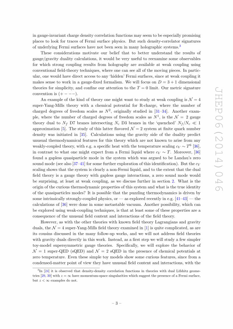
Transformation Properties in N = 2 sQED
Fields: ψ φ+ φ− η q+ q− λ χ a
U(1)e e−iαψ e+iαφ+ e−iαφ− η q+ q− λ χ a
U(1)i ψ φ+ φ− e−iαη e+iαq+ e−iαq− λ χ a
Table 2. Matter field transformation properties under the U(1)e and U(1)i symmetries.
Unfortunately, it turns out that once µ is turned on the scalars do not have a stable
ground state, since there are run-away directions in the scalar potential. The quickest way
to see this is to observe that minimizing Veff for a implies that a picks up a VEV
〈a〉 = − m√2g. (4.4)
Heuristically, apart from the surviving group of terms in the first line of eq. (4.2), the
potential for φ1,2, q1,2 is the same as the massless limit of the potential in the N = 1
case, for which there would be no stable solutions once µ > 0, even when a FI term is
present. The new terms demanded by N = 2 do not save the day if there is more than
one flavor hypermultiplet.
We have not figured out a way to prevent the emergence of run-away directions in the
scalar potential in two-flavor N = 2 sQED, but it is possible to get some insight into what
the supersymmetric interactions do to Fermi surfaces by modifying the theory above in
two simple ways:
A: Work with N = 2 sQED with only one flavor. This means giving up on electric
neutrality, and requires a hard breaking of supersymmetry to be sensible in the
infinite-volume limit, much as in section 3.3. We defer a discussion of this case in
section 4.3.
B: Keep the ion fields, but add some soft SUSY-breaking terms.
Given the title of this section, we proceed with option B, and work with a theory
defined by
L = LN= 2 +m2s
(|φ+|2 + |φ−|2 + |q+|2 + |q−|2
), (4.5)
where LN= 2 is the Lagrangian of N = 2 sQED with electron and ion superfields we
presented above, and ms is the soft SUSY-breaking mass.
Minimizing the softly-broken scalar potential with respect to a, we again get 〈a〉 =
− m√2g
. The condition for the remaining scalars to have a stable condensate is
m2s − g2ξ2 < µ2 < m2
s, (4.6)
where ms is the soft mass we introduced above. If the lower bound is violated none of
the scalars condense, while if the upper bound is violated there is a runaway direction. If
– 18 –

JHEP06(2014)046
eq. (4.6) is satisfied, the scalar VEVs must obey the relations
|φ+|2 + |q+|2 =µ2 − (m2
s − g2ξ2)
g2, |φ−| = |q−| = 0. (4.7)
Taking into account the electric neutrality constraint means that the scalar VEVs become
|φ+|2 = |q+|2 =µ2 − (m2
s − g2ξ2)
2g2, |φ−| = |q−| = 0. (4.8)
4.2 Search for a Fermi surface
The fermionic terms in the Lagrangian are the same as in eq. (3.18) together with the
additional terms
LN= 2|fermions = LN= 1|fermions +1
2χi/∂χ−
√2g(aψP−ψ + a†ψP+ψ + aηP−η + a†ηP+η
)−√
2g(φ−ψP−χ+ φ+χP−ψ + φ†−χP+ψ + φ†+ψP+χ
)(4.9)
−√
2g(q−ηP−χ+ q+χP−η + q†−χP+η + q†+ηP+χ
).
Again, once the scalars pick up VEVs, all of the fermionic fields mix with each other,
and seeing the effect of the chemical potential requires diagonalizing the kinetic operator.
To look for a Fermi surface, paralleling the approach of section 3.2, we introduce a single
column vector collecting all of our two-component spinors
Ψ =
ψLαψ†αRλαχ†α
ηLαη†αR
. (4.10)
This allows us to rewrite eq. (4.9) as
LN= 2|fermion = Ψ† ·MN= 2 ·Ψ, (4.11)
where
MN= 2 =
iσµ (∂µ − iµδµ0) 0 0 −g√
2φ†+ 0 0
0 iσµ (∂µ − iµδµ0) ig√
2φ†+ 0 0 0
0 −ig√
2φ+ iσµ∂µ 0 0 −ig√
2q+
−g√
2φ+ 0 0 iσµ∂µ −g√
2q+ 0
0 0 0 −g√
2q†+ iσµ (∂µ + iµδµ0) 0
0 0 ig√
2q†+ 0 0 iσµ (∂µ + iµδµ0)
.
(4.12)
Going to momentum space, calculating det(MN= 2) and setting p0 = 0, we obtain
det(MN= 2)|p0=0 = p2(4g2|φ+|2 − µ2 + p2
)2×(2g2|φ+|2(µ+ p) + (p− µ)
(2g2|q+|2 + p(µ+ p)
))×((p− µ)
(2g2|φ+|2 + p(µ+ p)
)+ 2g2|q+|2(µ+ p)
), (4.13)
– 19 –

JHEP06(2014)046
Figure 2. Left: Fermi momenta as a function of µ with g2ξ2
m2s
= 0.4. Right: Fermi momenta as a
function of µ with g2ξ2
m2s
= 0.6. The area between the dashed lines is the region where the scalars
are condensed and stable. Values of µ to the right of this region make the scalars unstable, while
to the left, the scalars are not condensed. Note that past g2ξ2 > m2s , where the scalars are always
condensed, there is no Fermi surface.
where we have used the charge neutrality relation between the scalar VEVs. If the scalars
condense, we can plug in eq. (4.8) to get
det(MN= 2)|p0=0 = p4(4g2|φ+|2 − µ2 + p2
)4= p4
(2[µ2 − (m2
s − g2ξ2)]− µ2 + p2)4
= p4(µ2 − 2m2
s + 2g2ξ2 + p2)4. (4.14)
Looking for a value of p 6= 0 which would make this vanish, we find that pF would have to
satisfy the relation
p2f = 2m2
s − µ2 − 2g2ξ2 !> 0. (4.15)
This relation will be satisfied if
µ2 < 2(m2s − g2ξ2). (4.16)
We are now in a position to classify all the things that can happen to the fermions in
this theory. To begin with, if
µ2 < m2s − g2ξ2, (4.17)
then the charged scalars do not condense. The fermion sector consists of massless gauginos
and massless matter fermions, which to leading order are free. Since the matter fermions
feel the chemical potential, there is a fermi surface at pF = µ. Since the charged scalars
are not condensed, the system is not a superconductor (before considering fermion pairing
effects), and it is natural to speculate that the physics in this regime resembles that of
conventional QED plasmas.
Next, if
m2s − g2ξ2 < µ2 < 2m2
s − 2g2ξ2 and µ2 < m2s, (4.18)
– 20 –

JHEP06(2014)046
the theory is stable, the charged scalars are condensed, so that the quantum liquid is a
superconductor, and there is a Fermi surface.
If
2m2s − 2g2ξ2 < µ2 < m2
s, (4.19)
the scalar sector is stable, with the charged scalars condensed and hence a broken U(1)Q,
so that the system is a superconductor. But now there is no Fermi surface.
Finally if
m2s < µ2, (4.20)
the scalar sector becomes unstable, and there does not appear to be a sensible finite-density
ground state.
To help visualize the behavior of the Fermi surfaces in this theory as a function the
parameters, see figure 2. As seen in the plots, as the scalar condensates get larger, the
Fermi momentum decreases. Naively, one could interpret figure 2 as implying that more
and more of the charge in the system leaks from the fermions into the scalars as µ is
increased enough to make the scalar condensate start growing. But see section 6 for a
result which suggests that this is not necessarily the case.
4.3 Non-supersymmetric cousin of N = 2 sQED
We now briefly return to Option A from section 4.1, where we start with N = 2 sQED
with one matter hypermultiplet, and delete the gauge fields just as in section 3.3 to avoid
problems with electric neutrality. This is a hard breaking of supersymmetry.
The scalar potential is now
V(0)
eff =∣∣∣√2ga+m
∣∣∣2 (|φ+|2 + |φ−|2)
+ 2g2|φ+|2|φ−|2
+g2
2
(|φ+|2 − |φ−|2 − ξ
)2− µ2
(|φ+|2 + |φ−|2
). (4.21)
The VEV of a is still given by eq. (4.4), but now there is a stable minimum for the other
scalar fields as well, as can be seen by rewriting the potential in the manner of eq. (3.8).
If ξ2 > 0, minimizing V(0)
eff leads to
|φ+|2 =µ2 + g2ξ2
g2, |φ−|2 = 0, (4.22)
while if ξ2 < 0, we get
|φ−|2 =µ2 − g2ξ2
g2, |φ+|2 = 0. (4.23)
(At ξ = 0, both scalar fields can condense, but for simplicity we do not consider this case
further.) As we have been saying, in this case there is no way to solve the charge neutrality
constraint within the scalar sector. If it were possible to adjust the chemical potential
which couples to the electrons independently from the one which couples to the selectrons,
– 21 –

JHEP06(2014)046
one could imagine that this electron chemical potential could be dialed in such a way that
the electrons would carry a charge density which precisely compensates that of the scalars.
But the structure of our supersymmetric theory does not allow us to introduce such an
independent chemical potential for the electrons, because the Yukawa interactions do not
respect the U(1) electron-number symmetry of the free action.
Hence, the solutions obtained in this section cannot yield an electrically-neutral back-
ground. Of course, since we have deleted the gauge fields from the theory with malice
aforethought, this is not a problem.
We now start the search for a Fermi surface for this non-supersymmetric theory. Again,
the diagonalization of the fermion sector after scalar condensation is much easier if we
switch to two-component notation. So long as ξ2 6= 0, LN= 2|fermions can be written in a
matrix notation without introducing Nambu-Gorkov spinors, but at ξ = 0 we expect all of
the scalar fields to develop non-trivial VEVs, making the analysis more involved. To keep
things as simple as possible, we only discuss the ξ2 6= 0 case in this paper. Moreover, as
our previous discussion makes clear, to understand what happens for ξ2 6= 0 we can focus
on ξ2 > 0.
Paralleling the approach of section 3.2, we introduce a single column vector collecting
all of the two-component spinors
Ψ(1) =
ψLαψ†αRλαχ†α
. (4.24)
We rewrite eq. (4.9) as
LN= 2|fermion = [Ψ(1)]† ·M (1)N=2 ·Ψ
(1), (4.25)
with
M(1)N= 2 =
iσµ (∂µ − iµδµ0) 0 0 −g
√2φ†+
0 iσµ (∂µ − iµδµ0) ig√
2φ†+ 0
0 −ig√
2φ+ iσµ∂µ 0
−g√
2φ+ 0 0 iσµ∂µ
. (4.26)
Computing the determinant of M(1)N= 2 in frequency-momentum space, we find that the
dispersion relations for the fermions are
p0 =1
2
(−µ±
√8g2φ2
+ + 4p2 ± 4pµ+ µ2
). (4.27)
But one can now check that there is no value of p2 = p2F > 0 such that there is a solution
to the equation above for p0 = 0. Thus there is no Fermi surface if we work with the
non-electrically-neutral state in the N = 2 theory with only one flavor hypermultiplet, or
in the healthy but non-supersymmetric theory with the gauge fields removed. Note the
contrast of this result with what we saw in section 3.3, where the analogous theory had a
Fermi surface.
– 22 –

JHEP06(2014)046
5 N = 2 sQED with a finite R-charge density
In this section, we will consider N = 2 sQED with one matter hypermultiplet. As we men-
tioned in the previous section, N = 1 sQED has a U(2) = U(1)R × SU(2)R R-symmetry
group. The U(1)R subgroup is anomalous, whereas the SU(2)R remains anomaly free.
We focus on the anomaly-free symmetry. The SU(2)R symmetry acts by matrix multi-
plication on the Weyl doublet (λα, χα) from the vector hypermultiplet and the charged
scalars (φ+, φ†−) from the matter hypermultiplet. The remaining fields in the theory are
SU(2)R singlets.
We can describe a system with a net R-charge by introducing a set of chemical po-
tentials µn for the R-symmetry charges. Any conserved charges Qn that one wishes to
introduce into the grand canonical partition function change the Hamiltonian by a shift
H → H−∑n
µnQn. (5.1)
However, the Qn charges must commute with each other in order to be simultaneously
observable. This means that Qn can only belong to the maximally commuting (Cartan)
sub-algebra of the non-Abelian algebra of the charge operators. In our case this must pick
a single U(1)R ⊂ SU(2)R to which we associate the chemical potential µR. Furthermore,
since this is a global un-gauged symmetry we do not have to worry about making the
system neutral with respect to U(1)R. Of course, we still have to make sure we maintain
electric neutrality!
Define the SU(2)R doublet fields
Φ ≡
(φ+
φ†−
), Ψα ≡
(λαχα
). (5.2)
Our anomaly-free U(1)R subgroup acts on these fields as
Φ→ eiατ3Φ, Ψα → eiατ3Ψα, (5.3)
where τ3 = σ3, the diagonal Pauli matrix.
Hence, the µR chemical potential enters the Lagrangian in the following way
L = (Ψα)†σµDµΨα + |DµΦ|2 + . . . , (5.4)
where we define9
DµΦ = ∂µ − iµRτ3δµ0 + igAµ, (5.5)
DµΨ = ∂µ − iµRτ3δµ0. (5.6)
The R-charge density is
QR = Ψ†σ0τ3Ψ + i[Φ† (∂0 − iµRτ3) τ3Φ− [(∂0 − iµRτ3) τ3Φ]†Φ
], (5.7)
9Recall that the fields in the vector hypermultiplet transform in the adjoint representation of the gauge
group, and hence are neutral under the Abelian U(1) gauge symmetry, while φ+, φ†− inside Φ have the same
non-zero electric charge.
– 23 –

JHEP06(2014)046
while the electric charge density is
QEM = i[Φ† (∂0 − iµRτ3) Φ− [(∂0 − iµRτ3) Φ]†Φ
]. (5.8)
For future reference, note that if φ+, φ− acquire identical time-independent VEVs, then
QR 6= 0, while QEM = 0. This is the key to ensuring that a finite R-charge density does
not violate the electric neutrality condition.
5.1 Scalar ground state
We look for time-independent scalar ground states, and work in unitary gauge, as we have
done throughout the paper. The bosonic potential with the µR contributions included is
V(0)
eff =∣∣∣√2ga+m
∣∣∣2 (|φ+|2 + |φ−|2)
+ 2g2 |φ+|2 |φ−|2 (5.9)
+g2
2
(|φ+|2 − |φ−|2 − ξ2
)2− µ2
R
(|φ+|2 + |φ−|2
),
where a is the scalar from the vector hypermultiplet. This theory always has a stable
non-trivial ground state when µR 6= 0, which can be seen from the fact that there is no
attractive |φ+|2|φ−|2 term in the potential. Just as before, a picks up the VEV
〈a〉 = − m√2g, (5.10)
which is independent of ξ. We will see below that charge neutrality requires that we set
ξ2 = 0, so we drop ξ from here onwards. Minimizing the scalar potential for the remaining
fields we find the condition
|φ+|2 + |φ−|2 =µ2R
g2. (5.11)
To see the consequences of electric neutrality, recall that φ†− feels a chemical potential −µRcompared to the field φ+ which feels a chemical potential µR. Recalling the expression for
the electric charge density, it is clear that electric neutrality in the scalar sector will be
ensured if they have the same VEVs,10 leading to
|φ+|2 = |φ−|2 =µ2R
2g2. (5.12)
Since these VEVs are non-zero for µR 6= 0, and the scalars are charged, the U(1) electro-
magnetic symmetry is broken, and the system is a superconductor. Of course, the charged
scalars also transform non-trivially under U(1)R, so the R symmetry is also spontaneously
broken once they develop VEVs. Indeed, since both scalars develop VEVs, the R symmetry
is completely broken.
10If we had allowed ξ 6= 0, then the masses would of φ− and φ+ would be split, and this argument would
not work.
– 24 –

JHEP06(2014)046
5.2 Search for a Fermi surface
Paralleling the approach of the preceding sections, we again introduce a single column
vector collecting all of the two-component spinors
ΨR =
ψLαψRαλ†α
χ†α
, (5.13)
and rewriting eq. (4.9) as
LN= 2|fermion = [ΨR]† ·MRN=2 ·ΨR. (5.14)
Now, of course, the structure of MRN= 2 is different, since the gauginos feel the R-charge
chemical potential, and the matter fermions are rendered effectively massless through the
VEV of a, so that
MRN=2 =
iσµ∂µ 0 ig
√2φ− −g
√2φ†+
0 iσµ∂µ −ig√
2φ+ −g√
2φ†−−ig√
2φ†− ig√
2φ†+ σµ (i∂µ − µRδµ0) 0
−g√
2φ+ −g√
2φ− 0 σµ (i∂µ + µRδµ0)
. (5.15)
Once we set φ+ = φ− = φ in view of eq. (5.12), the determinant of MRN= 2 takes a relatively
simple form. In fact, we find it instructive to write in two different ways. One way to write
it is
detMRN= 2 =
([p2
0 − p2] [
(p0 + µR)2 − p2]
+ 8g2|φ|2[p2 − p0(p0 + µR)
]+ 16g4|φ|4
)×([p2
0 − p2] [
(p0 − µR)2 − p2]
+ 8g2|φ|2[p2 − p0(p0 − µR)
]+ 16g4|φ|4
).
(5.16)
This form makes it easy to see that the g2|φ|2 = 0 consistency check is satisfied, where the
determinant must reduce to one expected for four massless Weyl fermions, two without
chemical potentials, and two with opposite-sign chemical potentials. But the dispersion
relations for g2|φ|2 6= 0 are hard to see in this form.
The other way to write detMRN= 2 is
detMRN= 2 =
4∏i=1
[(p0 − µi)2 − (|~p|+ κi)
2 + 4g2|φ|2], (5.17)
where
µ1,2 = µR/2, µ3,4 = −µR/2 and κ1,3 = µR/2, κ2,4 = −µR/2. (5.18)
This makes the form of the g2|φ|2 6= 0 dispersion relations for the eigenmodes manifest.
These dispersion relations are simple but quite unusual.
– 25 –

JHEP06(2014)046
Setting p0 = 0 to look for a Fermi surface, we find
detMRN= 2|p0=0 =
(p4 − p2
(µ2R − 8g2|φ|2
)+ 16g4|φ|4
)2. (5.19)
If g2|φ|2 were zero, then there would be a Fermi surface at p2F = µ2. For general g2|φ|2,
the Fermi momentum would have to satisfy the relation
p2F =
1
4
(µR ±
√µ2R − 16g2|φ|2
)2
> 0. (5.20)
In N = 2 sQED, minimizing the scalar potential leads to a VEV |φ|2 = µ2R/(2g
2). As
a result
detMRN= 2|p0=0 =
(4µ4
R + p4 + 3µ2Rp
2)2, (5.21)
which has no real zeros. Hence the fermions in N = 2 sQED with a chemical potential for
R-charge do not have a Fermi surface.
It is important to realize that the general structure of the fermion interaction terms
in this theory is, in and of itself, compatible with the existence of Fermi surfaces, even
after U(1) breaking. What prevents a Fermi surface for the fermions from appearing is the
precise relationship between the normalization of the Yukawa terms and the scalar self-
interaction terms, which is dictated by supersymmetry. To see this, consider modifying
the Yukawa couplings by changing g → gε and leaving everything else, including the scalar
sector, unchanged. When ε = 1, the theory is supersymmetric, but not otherwise. The
potential Fermi momenta are then modified to
p2F =
µ2R
4
(1±
√1− 8ε2
)2> 0. (5.22)
Tuning ε ≤ 1/(2√
2) < 1, a Fermi surface appears. Of course, in N = 2 sQED, we are not
allowed to vary the Yukawa couplings independently of the scalar potential, and we are
stuck with ε = 1, where there is no Fermi surface.
6 Fermion charge density without a Fermi surface
In the preceding sections we have seen that supersymmetric gauge theories and their cousins
often do not have Fermi surfaces, despite the fact that the chemical potential couples to the
fermions. How should this result be interpreted? Perhaps the simplest interpretation is that
in the Fermi-surface-less examples all of the charge which would normally be stored by the
fermions ‘leaks out’ into the scalars through the Yukawa couplings.11 In this scenario, when
the fermions have no Fermi surface, the charge density would only receive contributions
from the scalar fields.
In this section we show that this interpretation cannot be correct in general by explicitly
computing the charge density Q in a theory with fermions and scalars where no Fermi
surface develops at finite µ. The theory we consider in this section is chosen to make the
11We are very grateful to Julian Sonner for discussions which prodded us to explore this issue.
– 26 –

JHEP06(2014)046
calculation of the fermion contribution to Q particularly simple. We will see that this
contribution is non-vanishing.
The general idea of the calculation is to evaluate the T → 0 limit of the fermion
contribution to the ‘grand potential’ Ω = u − Ts − µQ, where u is the internal energy
density, s is the entropy density, and Q is the particle number density. Of course, Ω also
obeys the relation
Ω = −TV
logZ, (6.1)
where Z is the grand canonical partition function, T is the temperature, and V is the
volume of the system. Then we observe that the contributions to Ω can generically be split
into a contribution from fermionic energy eigenmodes plus a contribution from bosonic
energy eigenmodes, so that
Ω = −Ωfermions + Ωbosons, (6.2)
where the minus sign accounts for fermionic statistics when evaluating the fermion deter-
minant in Z. We write Ωfermions and Ωbosons as
Ωfermions =∑
i∈ particles, antiparticles
∫d3p
(2π)3
Ep,i2
+∑
i∈ particles
T
∫d3p
(2π)3log[1 + e−(Ep,i−µ)/T
]+
∑i∈ antiparticles
T
∫d3p
(2π)3log[1 + e−(Ep,i+µ)/T
], (6.3)
Ωbosons =∑
i∈ particles, antiparticles
∫d3p
(2π)3
Ep,i2
+∑
i∈ particles
T
∫d3p
(2π)3log[1− e−(Ep,i−µ)/T
]+
∑i∈ antiparticles
T
∫d3p
(2π)3log[1− e−(Ep,i+µ)/T
]. (6.4)
The dispersion relations Ep,i one should use above are the ones appropriate to the interact-
ing theory. The forms above follow from a number of formalisms, with standard statistical
mechanics arguments being perhaps the most physically transparent.12 The charge density
can now be defined as
Q = −∂Ω
∂µ. (6.5)
Note that the quantity Q defined in this way makes sense even when symmetry associated
to µ is spontaneously broken, as in the case of interest below. (Essentially, in the condensed
case, QV is the charge carried by a macroscopic lump of condensate with volume V .)
12Another way to obtain eq. (6.4) is to observe that e.g. Ω|fermion = −T logZ|fermion = −tr logMD, where
MD is the appropriate Dirac operator taking into account interaction corrections to the fermion propagators,
compute the trace log using one’s choice of finite-T formalisms, Matsubara or Schwinger-Keldysh, and then
take the T = 0 limit. Or one may use a T = 0 pole prescription (which is derived from the results of the
finite-T approach) to evaluate the trace log directly at T = 0. No matter the formalism, the result is of
course the same.
– 27 –
JHEP06(2014)046
We define the fermion contribution to Q as
Qfermions = −∂Ωfermions
∂µ. (6.6)
So to compute Qfermions for the theory we are interested in, we must first evaluate Ωfermions,
then take a derivative.
The theory we will focus on has two Majorana fermions λ, χ, one Dirac fermion ψ,
and one complex scalar φ, with interactions defined by the Lagrangian
L =1
2λ (i/∂ + µγ0)λ+
1
2χ(i/∂ − µγ0
)χ+ ψi/∂ψ + | (∂µ + iµδµ,0)φ|2
+ igε(φ†ψP−λ− φ†λP−ψ − φλP+ψ + φψP+λ
)− gε
(φψP−χ+ φχP−ψ + φ†χP+ψ + φ†ψP+χ
)− g2
2|φ|4 + LCT, (6.7)
where g and ε are dimensionless parameters characterizing the relative strengths of the
scalar self-interactions versus the Yukawa interactions, while µ is a chemical potential for
a U(1) symmetry acting as φ → e+iαφ, λ → e−iαλ, χ → e+iαχ. Finally, LCT collects the
counter-terms necessary to renormalize the theory
LCT = (δΛcc)4 + (δm)2|φ|2 + . . . , (6.8)
and we have written only the vacuum energy (δΛcc) and scalar mass (δm)2 counter-terms
explicitly since it turns out that they are the only ones we will need to compute Qfermions
to the order to which we work.
Our choice of the theory described by eq. (6.7) is inspired by N = 2 super-QED with a
single matter hypermultiplet with mass m and a U(1)R chemical potential µR. Specifically,
the version of eq. (6.7) with ε = 1 can be obtained from the N = 2 theory by the relations
Aµ = 0, φ+ = φ− = φ/√
2, a = −m/(g√
2), and µR = µ. For our purposes in this section,
the case ε = 1/√
2 will turn out to be the easiest to analyze. From the discussion at the
end of section 5.2, it follows that the fermions in the theory we consider in this section have
no Fermi surface so long as ε > 1/(2√
2), and this is the regime we focus on in this section.
Before looking at the interesting examples of what happens when ε > 1/(2√
2), we
quickly review the textbook calculation of the charge density Q carried by a non-interacting
Dirac fermion with a chemical potential µ, which help us stay oriented during calculations
in the interacting theory, which work out in an unusual way. Following the discussion
above, we write
−Ω(T, µ)Dirac = 4
∫d3p
(2π)3
Ep2
+ 2T
∫d3p
(2π)3log[1 + e−(Ep−µ)/T
]+ 2T
∫d3p
(2π)3log[1 + e−(Ep+µ)/T
],
(6.9)
where Ep =√p2 +m2 is the free-fermion dispersion relation. The first term is known as
the ‘vacuum’ contribution, while the second two terms are the ‘matter’ and ‘anti-matter’
contributions respectively. The factor of 4 on the vacuum term counts the total number
– 28 –

JHEP06(2014)046
of degrees of freedom (spin up and spin down particle and anti-particle modes), and the
factors of 2 on the matter terms have the same origin, accounting for the spin up and down
contributions. In the zero-temperature limit, and with µ > 0, this reduces to
−Ω(µ)Dirac = 4
∫d3p
(2π)3
Ep2
+ 2
∫d3p
(2π)3(µ− Ep)θ(µ− Ep), (6.10)
where θ is the Heaviside step function, and θ(µ−Ep) = θ(pF ). Of course, the anti-fermion
contribution has dropped out at T = 0.
For the free Dirac fermion, the ‘vacuum’ term is obviously independent of µ, and is
irrelevant for the charge density. Setting m = 0 for simplicity and evaluating the remaining
‘matter’ term we obtain
−Ω(µ)Dirac =µ4
12π2⇒ QDirac =
µ3
3π2, (6.11)
which is the standard result [69].
We now turn to the calculation of the fermion contribution to Q in the toy theory
described by eq. (6.7). From eq. (5.17) and eq. (5.18), we see that we have four eigen-
modes contributing to Ω, with
E2p,i ≡ (|~p|+ κi)
2 + 2ε2g2|φ|2, i = 1, 2, 3, 4, (6.12)
with the i-th mode having the chemical potential µi, but now we have |〈φ〉|2 = µ2/g2.13
Note that µi with i = 1, 2 are positive, while µi with i = 3, 4 are negative for µ > 0. Also,
we observe that eq. (6.12) describes eight fermionic degrees of freedom, since we have four
Weyl fermions coupled to each other when ε 6= 0.
These dispersion relations are highly unusual, and are a consequence of the spontaneous
U(1) breaking driven by scalar condensation communicated to the fermions through the
Yukawa couplings with strength set by ε.14 Hence in addition to exploring the behavior
of the ε = 1/√
2 theory, we also verify that the ε → 0 limit yields the expected free-
fermion results.
We now write down the fermionic contribution to Ω, working with general ε for the
moment. Note that in view of the signs on the µi’s, when writing down the matter con-
tributions to Ω at T = 0 we must take into account the particle contributions for the first
two modes, while for the second two modes we have to take into account the antiparticle
contributions. Adding up the contributions, we get
−Ω(µ)|fermion =
4∑i=1
2×∫
d3p
(2π)3
Ep,i2
+
2∑i=1
∫d3p
(2π)3(µi − Ep,i) θ(µi − Ep,i) (6.13)
+
4∑i=3
∫d3p
(2π)3(−µi − Ep,i) θ(−µi − Ep,i).
13The normalization of φ used in this section differs from the one used in section 5, with φhere = φthere/2,
so that the kinetic term of φhere in eq. (6.7) is canonically-normalized.14It may also be interesting to explore why happens if the U(1) symmetry is broken both spontaneously
and explicitly, by U(1)-violating mass terms. However, the dispersion relations become very complicated
in this case, and the integrals determining the fermion contribution to grand potential Ω appear to become
analytically intractable. We leave an exploration of combined spontaneous and explicit U(1) breaking effects
to future work.
– 29 –

JHEP06(2014)046
We begin by making sure that the ε → 0 limit of −Ω|fermions behaves as expected
in view of the fact that at ε = 0 no spontaneous U(1) breaking is communicated to the
fermions. In the ε→ 0, we know that the fermionic part of the theory described by eq. (6.7)
becomes a theory of a single free massless Dirac fermion that feels a chemical potential µ,
and two free Weyl fermions which do not feel the chemical potential. So as ε→ 0, we must
recover get eq. (6.11). As already noted in section 5.2, the dispersion relations in eq. (6.12)
behave in a very peculiar way in this limit, so the way the consistency check is satisfied
is surprisingly subtle. Evaluating eq. (6.14) and taking the ε→ 0 limit, and canceling the
standard UV-divergent vacuum energy contribution by adjusting the δΛcc counter-term,
we find that
−Ω(µ)fermion =
(µ4
96π2+ 2× 7µ4
192π2
)=
µ4
12π2, (6.14)
which matches eq. (6.11) as advertised. The unusual thing is that the first piece above
comes from the vacuum term, while the second comes from the matter and anti-matter
terms. The fact that the vacuum term makes a µ-dependent contribution to Ω may seem
strange, but it is a consequence of the peculiar way we must write the dispersion relations
at ε = 0 to keep them diagonal when ε > 0.
Now consider the same calculation when ε > 1/(2√
2). The ‘matter’ terms in eq. (6.14)
vanish, which is the expected signature of the lack of a Fermi surface. The ‘vacuum’
contributions have UV divergences, as is usually the case, and must be regulated and
renormalized. For our purposes here, a simple momentum cutoff regulator Λ is sufficient,
since we are considering a Yukawa theory, see eq. (6.7), which is a classic case where cutoff
regularization is particularly efficient.15 We obtain
−Ωfermion =Λ4
2π2+ε2|φ|2Λ2
π2
+
[µ4
96π2+
1
2π2ε2|φ|2
(1
2ε2|φ|2 − µ2
)− 1
2π2ε2|φ|2 log(2)
(2ε2|φ|2 − µ2
R
)+
1
4π2ε2|φ|2
(2ε2|φ|2 − µ2
R
)log
(8ε2|φ|2
Λ2
)]. (6.15)
15Dimensional regularization (DR) is also often an efficient regulator. However, the highly unusual
Lorentz-breaking dispersion relations that result after symmetry breaking make the standard DR formulas
inapplicable. Rather than common Gamma functions the analytically-continued integrals have to be written
in terms of Appell functions (hypergeometric functions in two variables) in DR. However, the necessary
asymptotic expansions of these functions are extremely complicated. We were able to find verifiably-correct
expressions for the relevant asymptotics in some recent mathematics literature [70], but these expressions
are very cumbersome to work with. It may be an interesting project in mathematical physics to figure out a
way to obtain sufficiently transparent closed-form expressions for the asymptotics of these special functions
for using them in QFT calculations, but it is beyond the scope of the present work. In any case, it is a
standard principle of quantum field theory that if one obtains a finite and cut-off independent expression
for an observable, using a systematic regularisation and renormalisation procedure, any other regulator
would give the same final expression. However, at intermediate stages the calculation may become more
or less difficult depending on the regulator chosen, and so in the interests of simplicity we stick to cutoff
regularization.
– 30 –

JHEP06(2014)046
The power-law divergences above (together with any other ones coming from the non-
fermion parts of Ω) are trivially cancelled off by appropriate cosmological constant and
scalar mass counter-terms from eq. (6.8). For generic ε, one also has to turn on |φ|4 counter-
terms at this order, and this would lead to the need to renormalize g to compute Qfermions.
However, if we consider a theory with ε = 1/√
2, then on the one hand there is still
no Fermi surface since 1/√
2 > 1/(2√
2). On the other hand, at the order to which we
work above there are no logarithmic divergences proportional to |φ|2 or |φ|4. Hence in the
theory with ε = 1/√
2 we do not need to introduce a |φ|4 counter-term and renormalize
g to compute Qfermions to leading order. Since consideration of the theory described by
eq. (6.7) with ε = 1/√
2 is sufficient to make our point, we set
ε = 1/√
2 (6.16)
from here onward.
We are now in a position to write down the renormalized expression for Ωfermion:
−Ωfermion|ε=1/√
2 = −17µ4
96π2⇒ Qfermion|ε=1/
√2 = −17µ3
24π26= 0. (6.17)
Note that this has the same parametric dependence on µ as eq. (6.11), but a different
numerical coefficient. Looking back at eq. (5.7) for the total U(1)R charge, we see that in
the ε = 1/√
2 theory it is
Q|ε=1/√
2 =2µ3
g2− 17µ3
24π2+ . . . , (6.18)
where the first term is the tree-level scalar contribution from the scalars, the second is the
leading fermion contribution,16 and the ellipsis denotes the one-loop scalar contribution
and higher order terms. This example shows that fermions can contribute to a charge
density Q, as defined by eq. (6.6), even when there is no Fermi surface. We emphasize
that this unusual result is obtained in the unusual situation where the U(1) symmetry
associated to Q is spontaneously broken due to scalar condensation. For this reason,
there is no conflict with Luttinger’s theorem, which relates Qfermions to the volume of
the Fermi surface, because Luttinger’s theorem assumes that the U(1) symmetry is not
spontaneously broken.
Before closing this section, we find it illuminating to discuss how our results would be
modified in a theory with a more complicated mass matrix. In any free theory with fermion-
number symmetry preserving Dirac masses, the mass matrix can always be diagonalised by
a linear transformation of fields with the same charge under the symmetries of the theory.
After this procedure, the system is equivalent to one with free massive Dirac fermions
that feel a chemical potential. The dispersion relation for the mode i, with mass mi that
experiences a chemical potential µi is then given by
(Ei − µi)2 = m2i . (6.19)
16As usual, the fermion contribution comes from a one-loop calculation, just as in the free case: fermions
are intrinsically quantum objects.
– 31 –

JHEP06(2014)046
Consequently, the charge of the system is necessarily stored in Fermi surfaces, which would
appear if there are modes with µi > mi. The same statement would apply in any weakly-
interacting system in which the interactions do not produce effective mass terms which
break the fermion number symmetries. Such systems satisfy the assumptions that go into
Luttinger’s theorem, and their behavior will necessarily follow its predictions. Symmetry
preserving masses can never lead to dispersion relations of the form of eq. (6.12), and in
particular the term g2φ2 in eq. (6.12) cannot simply be replaced by m2D, where mD is a
Dirac mass.
The ‘mass terms’ that arise as a result of a scalar VEV in the Lagrangian (6.7) spon-
taneously break the U(1) R-symmetry. For example, the term igε⟨φ†⟩ψP−λ couples (a
component of) the state λ, which is charged under the symmetry, to ψ, which is uncharged.
The only way to write down a mass term which appears in the non-standard dispersion re-
lations in the same way as g2|φ|2 does, without spontaneous symmetry breaking, is through
explicit symmetry breaking. Such a mass means that the mass matrix cannot be diago-
nalised by a rotation of fields with the same charge, as opposed to in theories containing
only Dirac masses. This is not surprising, in light of the fact that such terms in the disper-
sion relations break the assumptions going into Luttinger’s theorem. Such mass terms may
arise from symmetry-breaking Majorana mass terms, which would be an explicit rather
than spontaneous breaking of the symmetry.
A potentially interesting calculation would be to find the charge stored in a system,
qualitatively different from N = 2 theories, which contain both symmetry-preserving Dirac
and symmetry-violating masses from spontaneous symmetry breaking by a scalar (or al-
ternatively, symmetry-breaking Majorana masses). However, the dispersion relations in
such systems are extremely complicated, and even in cases where closed forms for these
can be obtained, the integrals to evaluate the grand potential become very cumbersome.
It would be interesting to return to this problem in future, particularly in simple non-
supersymmetric theories where the dispersion relations may be tractable.
7 Discussion
The most familiar finite density low-temperature systems that involve chemical potentials
coupling to fermions are Fermi liquids. The applicability of Landau’s Fermi liquid theory
requires two basic features:
1. A Fermi surface, showing up as e.g. the locus in spatial momentum space where the
inverse fermion propagator vanishes when p0 = 0.
2. Having short-ranged-enough interactions amongst its degrees of freedom.
These two properties lead to the existence of well-defined quasiparticles and all of the
familiar Fermi liquid phenomenology like Landau’s zero sound, a specific heat linear in
temperature, and so on. Examples of theories which do not fit into this paradigm are
intrinsically interesting, and come about when one or both of these properties fail to hold.
Obviously, free systems satisfy both assumptions. Perhaps the simplest non-trivial
example of a non-Fermi liquid, which also happens to be relevant to our paper, is the
– 32 –

JHEP06(2014)046
non-supersymmetric electron plasma described by QED, which satisfies (1), but does not
satisfy (2), as reviewed in section 2. When there are strong attractive interactions among
the fermions, one can also easily imagine (1) failing due to the formation of bosonic bound
states. The bosonic states obviously do not have a Fermi surface, and at low temperature
would typically tend to Bose condense instead. If there are only parametrically weak
attractive interactions between the fermions, then while the fermion Green’s function will
have a sharp Fermi surface singularity at any finite order in perturbation theory, the
BCS mechanism generally leads to the formation of Cooper pairs and a non-perturbative
BCS gap ∆ ∼ µe−1/g µ ∼ pF . The Fermi surface then gets smeared out by a non-
perturbatively small amount ∆/pF 1. Systems showing both sorts of behavior are well
known, and have been explored in e.g. the context of the so-called BCS-BEC crossover in
cold atomic gases [46, 71]. Note that in both of these examples the U(1) particle number
symmetry of the fermions becomes broken by composite scalar condensation. Luttinger’s
theorem does not apply once this happens.
It is much less obvious to see how a Fermi surface could disappear in perturbation
theory, in the limit of of arbitrarily weak interactions, where one does not expect the
fermions to be able to form bosonic bound states. Indeed, so long as Luttinger’s theorem
is applicable, such a thing should not happen. But 4D supersymmetric theories always
have elementary scalar fields which couple to fermions, and these could condense even at
arbitrarily weak coupling. So for weakly coupled supersymmetric theories there is reason to
be concerned about the existence of Fermi surfaces. Our results indicate that at least some
theories with interactions of the types found in supersymmetric gauge theories fail to satisfy
(1) due to scalar condensation driving quadratic mixing between Dirac fermions, which
directly feel the chemical potential µ, and Majorana fermions, which do not. Luttinger’s
theorem does not apply because of scalar condensation which breaks the relevant U(1)
symmetry. There does not appear to be any modified Luttinger relation of sort explored
in [46] that one could define in supersymmetric QED, because of the lack of separate
fermionic and bosonic number symmetries.
Moreover, as explained in section 2, in supersymmetric QED, this mixing is order
unity even when the gauge coupling is arbitrarily small. In a sharp contrast with the other
examples in which Fermi surfaces are endangered by interactions, in supersymmetric QED
there is no parameter which we could tune smoothly to interpolate between a regime where
there is a perturbative Fermi surface to one where there is not. The physics at any g > 0 is
sharply different from the physics at g = 0. After the diagonalization which takes into ac-
count the scalar-condensate-induced mixing, the fermionic eigenmodes have highly peculiar
dispersion relations with a complex dependence on µ, and when the smoke clears we do not
see a Fermi surface in any of our supersymmetric examples. In our non-supersymmetric
examples, with hard and soft breaking of SUSY, where Luttinger’s theorem also does not
apply, whether a Fermi surface appears depends on the values of the parameters. Perhaps
this should not be surprising: just because Luttinger’s theorem is not available to shield the
Fermi surface from danger, this does not imply that interactions must destroy the Fermi
surface. This is illustrated by our non-supersymmetric examples in section 3.3 and part of
section 5.2, where the relevant U(1) is broken, but there is nevertheless a Fermi surface.
– 33 –

JHEP06(2014)046
But in our supersymmetric examples, it does turn out to be the case that turning on any
non-zero interaction, which results in the U(1) breaking, obliterates the Fermi surface. Fi-
nally, we again emphasize that our supersymmetric examples all led to superconducting
ground states, with the U(1) breaking driven by charged elementary scalar condensation,
as opposed to any sort of BCS-like fermion pairing mechanism.
Obviously, in this paper we have only managed to scratch the surface of a large pile
of interesting issues. Sticking with super-QED, or the sort of non-supersymmetric theo-
ries we considered in this paper, one can ask many questions. For instance, what is the
quasiparticle spectrum of such theories? What are the thermodynamics? Perhaps the most
conceptually interesting question is whether the fermions manage to store any of the charge
density, despite not having a Fermi surface. Relatedly, can one develop a useful heuristic
understanding of the reason for the disappearance of the Fermi surface? Naively, it may
have seemed that the most natural possibility is that when there is no Fermi surface, all
of the charge ‘leaks out’ of the fermion sector through the Yukawa terms, and gets stored
by the scalars. But in section 6, we explicitly calculated the fermion contribution to the
charge density in an example where there is no Fermi surface, and showed that the fermion
contribution to the charge density is non-vanishing. We do not yet know a heuristic physi-
cal interpretation for this result, which seems to go against the conventional wisdom about
how fermions behave at finite density. Of course, this conventional wisdom is based on
Luttinger-theorem-inspired pictures, and as we have emphasized Luttinger’s theorem does
not apply to our condensed-scalar examples.
If one bravely hopes to try to make direct contact with condensed matter physics, it
may perhaps be prudent to start by attacking the questions we raised above in Abelian
gauge theory, since examples of dynamical Abelian gauge fields coupled to fundamental and
emergent matter of various statistics are ubiquitous in condensed matter. Perhaps there
are condensed matter systems for which theoretical models involving Yukawa interactions
of the sort seen in SUSY gauge theories may be useful.
To make contact with the results of gauge-gravity duality, it is important to generalize
our analysis to include non-Abelian gauge fields, and to begin working with theories that
actually have gravity duals at strong coupling. The details of the scalar stabilization
mechanisms may well be different, and presumably do not involve turning on FI terms
(but see [72]), as we had to do here in a number of examples. An interesting issue is
that from the weak-coupling side, it seems likely that finite density would drive squark
condensation, but this would lead to gauge symmetry breaking, which has not been seen
in most systems at strong coupling. (Of course, signs of breaking of global symmetries
are ubiquitous in gauge-gravity duality.) Also, instead of electrical neutrality, in weak-
coupling treatments of non-Abelian gauge theories presumably a starring role would be
played by color neutrality, as has been the case in studies of high density QCD. Once the
generalization to non-Abelian theories is performed, one would have the opportunity to
investigate many interesting phenomenological and conceptual questions. Is the charge
typically stored in fermions, or in the scalars? The possibility that in some cases it may
be stored in scalar condensates has been noted in the AdS/CFT context in e. g. [39, 73].
Are there actually Fermi surfaces at weak coupling in theories that do not seem to have
– 34 –

JHEP06(2014)046
one holographically? Are there examples of theories with the opposite behavior — Fermi-
surface like singularities at strong coupling, but no Fermi surfaces at weak coupling?
We hope to return to some of these questions in future work.
Acknowledgments
We are deeply indebted to Andy O’Bannon and Julian Sonner for collaboration at the
initial stages of this work, and are very grateful to them for detailed and thoughtful com-
ments on the manuscript. We also thank Paulo Bedaque, Tom Cohen, Jason Evans, Sean
Hartnoll, Nabil Iqbal, Peter Koroteev, John March-Russell, Janos Polonyi, Subir Sachdev,
Fidel Schaposnik, Andrei Starinets, and David Tong for inspirational discussions. We are
especially grateful to David Tong for his prescient skepticism regarding our original naive
assumption that Fermi surfaces would surely survive the addition of SUSY interactions.
We acknowledge support from U.S. DOE grant FG02-94ER40823 (A. C.), the Graduate
Scholarship of St. John’s College, Oxford (S. G.), and STFC (E. H.).
Open Access. This article is distributed under the terms of the Creative Commons
Attribution License (CC-BY 4.0), which permits any use, distribution and reproduction in
any medium, provided the original author(s) and source are credited.
References
[1] J.M. Maldacena, The large-N limit of superconformal field theories and supergravity, Adv.
Theor. Math. Phys. 2 (1998) 231 [Int. J. Theor. Phys. 38 (1999) 1113] [hep-th/9711200]
[INSPIRE].
[2] S.A. Hartnoll, Lectures on holographic methods for condensed matter physics, Class. Quant.
Grav. 26 (2009) 224002 [arXiv:0903.3246] [INSPIRE].
[3] J. McGreevy, Holographic duality with a view toward many-body physics, Adv. High Energy
Phys. 2010 (2010) 723105 [arXiv:0909.0518] [INSPIRE].
[4] N. Iqbal, H. Liu and M. Mezei, Lectures on holographic non-Fermi liquids and quantum
phase transitions, arXiv:1110.3814 [INSPIRE].
[5] A. Karch and E. Katz, Adding flavor to AdS/CFT, JHEP 06 (2002) 043 [hep-th/0205236]
[INSPIRE].
[6] J.P. Gauntlett, J. Sonner and T. Wiseman, Holographic superconductivity in M-theory, Phys.
Rev. Lett. 103 (2009) 151601 [arXiv:0907.3796] [INSPIRE].
[7] J.P. Gauntlett, J. Sonner and T. Wiseman, Quantum criticality and holographic
superconductors in M-theory, JHEP 02 (2010) 060 [arXiv:0912.0512] [INSPIRE].
[8] S.S. Gubser, C.P. Herzog, S.S. Pufu and T. Tesileanu, Superconductors from superstrings,
Phys. Rev. Lett. 103 (2009) 141601 [arXiv:0907.3510] [INSPIRE].
[9] S.-S. Lee, A non-Fermi liquid from a charged black hole: a critical Fermi ball, Phys. Rev. D
79 (2009) 086006 [arXiv:0809.3402] [INSPIRE].
[10] H. Liu, J. McGreevy and D. Vegh, Non-Fermi liquids from holography, Phys. Rev. D 83
(2011) 065029 [arXiv:0903.2477] [INSPIRE].
– 35 –

JHEP06(2014)046
[11] M. Edalati, J.I. Jottar and R.G. Leigh, Shear modes, criticality and extremal black holes,
JHEP 04 (2010) 075 [arXiv:1001.0779] [INSPIRE].
[12] M. Edalati, J.I. Jottar and R.G. Leigh, Holography and the sound of criticality, JHEP 10
(2010) 058 [arXiv:1005.4075] [INSPIRE].
[13] S.A. Hartnoll and A. Tavanfar, Electron stars for holographic metallic criticality, Phys. Rev.
D 83 (2011) 046003 [arXiv:1008.2828] [INSPIRE].
[14] S.A. Hartnoll, D.M. Hofman and D. Vegh, Stellar spectroscopy: fermions and holographic
Lifshitz criticality, JHEP 08 (2011) 096 [arXiv:1105.3197] [INSPIRE].
[15] J.P. Gauntlett, J. Sonner and D. Waldram, Spectral function of the supersymmetry current,
JHEP 11 (2011) 153 [arXiv:1108.1205] [INSPIRE].
[16] J.P. Gauntlett, J. Sonner and D. Waldram, Universal fermionic spectral functions from
string theory, Phys. Rev. Lett. 107 (2011) 241601 [arXiv:1106.4694] [INSPIRE].
[17] R. Belliard, S.S. Gubser and A. Yarom, Absence of a Fermi surface in classical minimal
four-dimensional gauged supergravity, JHEP 10 (2011) 055 [arXiv:1106.6030] [INSPIRE].
[18] L. Huijse and S. Sachdev, Fermi surfaces and gauge-gravity duality, Phys. Rev. D 84 (2011)
026001 [arXiv:1104.5022] [INSPIRE].
[19] L. Huijse, S. Sachdev and B. Swingle, Hidden Fermi surfaces in compressible states of
gauge-gravity duality, Phys. Rev. B 85 (2012) 035121 [arXiv:1112.0573] [INSPIRE].
[20] S. Sachdev, A model of a Fermi liquid using gauge-gravity duality, Phys. Rev. D 84 (2011)
066009 [arXiv:1107.5321] [INSPIRE].
[21] N. Ogawa, T. Takayanagi and T. Ugajin, Holographic Fermi surfaces and entanglement
entropy, JHEP 01 (2012) 125 [arXiv:1111.1023] [INSPIRE].
[22] S.A. Hartnoll and E. Shaghoulian, Spectral weight in holographic scaling geometries, JHEP
07 (2012) 078 [arXiv:1203.4236] [INSPIRE].
[23] T. Faulkner and N. Iqbal, Friedel oscillations and horizon charge in 1D holographic liquids,
JHEP 07 (2013) 060 [arXiv:1207.4208] [INSPIRE].
[24] R.J. Anantua, S.A. Hartnoll, V.L. Martin and D.M. Ramirez, The Pauli exclusion principle
at strong coupling: Holographic matter and momentum space, JHEP 03 (2013) 104
[arXiv:1210.1590] [INSPIRE].
[25] S. Sachdev, Compressible quantum phases from conformal field theories in 2 + 1 dimensions,
Phys. Rev. D 86 (2012) 126003 [arXiv:1209.1637] [INSPIRE].
[26] O. DeWolfe, S.S. Gubser and C. Rosen, Fermi surfaces in maximal gauged supergravity,
Phys. Rev. Lett. 108 (2012) 251601 [arXiv:1112.3036] [INSPIRE].
[27] O. DeWolfe, S.S. Gubser and C. Rosen, Fermi surfaces in N = 4 super-Yang-Mills theory,
Phys. Rev. D 86 (2012) 106002 [arXiv:1207.3352] [INSPIRE].
[28] S.A. Hartnoll, J. Polchinski, E. Silverstein and D. Tong, Towards strange metallic
holography, JHEP 04 (2010) 120 [arXiv:0912.1061] [INSPIRE].
[29] P. Koroteev and M. Libanov, On existence of self-tuning solutions in static braneworlds
without singularities, JHEP 02 (2008) 104 [arXiv:0712.1136] [INSPIRE].
[30] S. Kachru, X. Liu and M. Mulligan, Gravity duals of Lifshitz-like fixed points, Phys. Rev. D
78 (2008) 106005 [arXiv:0808.1725] [INSPIRE].
– 36 –

JHEP06(2014)046
[31] S.S. Gubser, Thermodynamics of spinning D3-branes, Nucl. Phys. B 551 (1999) 667
[hep-th/9810225] [INSPIRE].
[32] R.-G. Cai and K.-S. Soh, Critical behavior in the rotating D-branes, Mod. Phys. Lett. A 14
(1999) 1895 [hep-th/9812121] [INSPIRE].
[33] A. Chamblin, R. Emparan, C.V. Johnson and R.C. Myers, Charged AdS black holes and
catastrophic holography, Phys. Rev. D 60 (1999) 064018 [hep-th/9902170] [INSPIRE].
[34] M. Cvetic and S.S. Gubser, Phases of R charged black holes, spinning branes and strongly
coupled gauge theories, JHEP 04 (1999) 024 [hep-th/9902195] [INSPIRE].
[35] S. Kobayashi, D. Mateos, S. Matsuura, R.C. Myers and R.M. Thomson, Holographic phase
transitions at finite baryon density, JHEP 02 (2007) 016 [hep-th/0611099] [INSPIRE].
[36] A. Karch, D.T. Son and A.O. Starinets, Zero sound from holography, arXiv:0806.3796
[INSPIRE].
[37] M. Kulaxizi and A. Parnachev, Comments on Fermi liquid from holography, Phys. Rev. D 78
(2008) 086004 [arXiv:0808.3953] [INSPIRE].
[38] C. Hoyos-Badajoz, A. O’Bannon and J.M.S. Wu, Zero sound in strange metallic holography,
JHEP 09 (2010) 086 [arXiv:1007.0590] [INSPIRE].
[39] M. Ammon et al., On stability and transport of cold holographic matter, JHEP 09 (2011) 030
[arXiv:1108.1798] [INSPIRE].
[40] R.A. Davison and A.O. Starinets, Holographic zero sound at finite temperature, Phys. Rev. D
85 (2012) 026004 [arXiv:1109.6343] [INSPIRE].
[41] M. Ammon, K. Jensen, K.-Y. Kim, J.N. Laia and A. O’Bannon, Moduli spaces of cold
holographic matter, JHEP 11 (2012) 055 [arXiv:1208.3197] [INSPIRE].
[42] H.-C. Chang and A. Karch, Novel solutions of finite-density D3/D5 probe brane system and
their implications for stability, JHEP 10 (2012) 069 [arXiv:1207.7078] [INSPIRE].
[43] F. Bigazzi, A.L. Cotrone and J. Tarrio, Charged D3-D7 plasmas: novel solutions, extremality
and stability issues, JHEP 07 (2013) 074 [arXiv:1304.4802] [INSPIRE].
[44] D. Yamada and L.G. Yaffe, Phase diagram of N = 4 super-Yang-Mills theory with
R-symmetry chemical potentials, JHEP 09 (2006) 027 [hep-th/0602074] [INSPIRE].
[45] S. Paik and L.G. Yaffe, Thermodynamics of SU(2) N = 2 supersymmetric Yang-Mills theory,
JHEP 01 (2010) 059 [arXiv:0911.1392] [INSPIRE].
[46] S. Powell, S. Sachdev and H.P. Buchler, Depletion of the Bose-Einstein condensate in
Bose-Fermi mixtures, Phys. Rev. B 72 (2005) 024534 [cond-mat/0502299].
[47] R. Harnik, D.T. Larson and H. Murayama, Supersymmetric color superconductivity, JHEP
03 (2004) 049 [hep-ph/0309224] [INSPIRE].
[48] M. Arai and N. Okada, Color superconductivity in N = 2 supersymmetric gauge theories,
Phys. Rev. D 74 (2006) 045004 [hep-th/0512234] [INSPIRE].
[49] A. Barranco and J.G. Russo, Supersymmetric BCS, JHEP 06 (2012) 104 [arXiv:1204.4157]
[INSPIRE].
[50] A. Barranco, Supersymmetric BCS: effects of an external magnetic field and spatial
fluctuations of the gap, JHEP 07 (2013) 172 [arXiv:1301.0691] [INSPIRE].
– 37 –

JHEP06(2014)046
[51] A.L. Fetter and J.D. Walecka, Quantum theory of many-particle systems, Dover Publications,
U.S.A. (1971).
[52] K. Iida and G. Baym, The superfluid phases of quark matter: Ginzburg-Landau theory and
color neutrality, Phys. Rev. D 63 (2001) 074018 [Erratum ibid. D 66 (2002) 059903]
[hep-ph/0011229] [INSPIRE].
[53] M. Alford and K. Rajagopal, Absence of two flavor color superconductivity in compact stars,
JHEP 06 (2002) 031 [hep-ph/0204001] [INSPIRE].
[54] A.W. Steiner, S. Reddy and M. Prakash, Color neutral superconducting quark matter, Phys.
Rev. D 66 (2002) 094007 [hep-ph/0205201] [INSPIRE].
[55] M.G. Alford, A. Schmitt, K. Rajagopal and T. Schafer, Color superconductivity in dense
quark matter, Rev. Mod. Phys. 80 (2008) 1455 [arXiv:0709.4635] [INSPIRE].
[56] T. Holstein, R.E. Norton and P. Pincus, De Haas-van Alphen effect and the specific heat of
an electron gas, Phys. Rev. B 8 (1973) 2649 [INSPIRE].
[57] M.Y. Reizer, Relativistic effects in the electron density of states, specific heat, and the
electron spectrum of normal metals, Phys. Rev. B 40 (1989) 11571 [INSPIRE].
[58] J. Gan and E. Wong, Non-Fermi-liquid behavior in quantum critical systems, Phys. Rev.
Lett. 71 (1993) 4226 [INSPIRE].
[59] S. Chakravarty, R.E. Norton and O.F. Syljuasen, Transverse gauge interactions and the
vanquished Fermi liquid, Phys. Rev. Lett. 74 (1995) 1423.
[60] G. Gabadadze and R.A. Rosen, Effective field theory for quantum liquid in dwarf stars,
JCAP 04 (2010) 028 [arXiv:0912.5270] [INSPIRE].
[61] G. Gabadadze and D. Pirtskhalava, Quantum liquid signatures in dwarf stars, JCAP 05
(2009) 017 [arXiv:0904.4267] [INSPIRE].
[62] G. Gabadadze and R.A. Rosen, Charged condensate and helium dwarf stars, JCAP 10
(2008) 030 [arXiv:0806.3692] [INSPIRE].
[63] P.F. Bedaque, E. Berkowitz and A. Cherman, Nuclear condensate and helium white dwarfs,
Astrophys. J. 749 (2012) 5 [arXiv:1111.1343] [INSPIRE].
[64] G. Baym and S.A. Chin, Landau theory of relativistic Fermi liquids, Nucl. Phys. A 262
(1976) 527 [INSPIRE].
[65] T. Rube and J.G. Wacker, The simplicity of perfect atoms: degeneracies in supersymmetric
hydrogen, J. Math. Phys. 52 (2011) 062102 [arXiv:0912.2543] [INSPIRE].
[66] C.P. Herzog and T. Klose, The perfect atom: bound states of supersymmetric quantum
electrodynamics, Nucl. Phys. B 839 (2010) 129 [arXiv:0912.0733] [INSPIRE].
[67] S.R. Behbahani, M. Jankowiak, T. Rube and J.G. Wacker, Nearly supersymmetric dark
atoms, Adv. High Energy Phys. 2011 (2011) 709492 [arXiv:1009.3523] [INSPIRE].
[68] J.M. Luttinger, Fermi surface and some simple equilibrium properties of a system of
interacting fermions, Phys. Rev. 119 (1960) 1153 [INSPIRE].
[69] J. Kapusta and C. Gale, Finite-temperature field theory: principles and applications,
Cambridge University Press, Cambridge, U.K. (2006).
[70] C. Ferreira and J.L. Lopez, Asymptotic expansions of the Appell’s function F1, Quart. App.
Math. 62 (2004) 235.
– 38 –

JHEP06(2014)046
[71] Q. Chen, J. Stajic, S. Tan and K. Levin, Bcs-bec crossover: from high temperature
superconductors to ultracold superfluids, Phys. Rep. 412 (2005) 1.
[72] M. Ammon, J. Erdmenger, S. Hohne, D. Lust and R. Meyer, Fayet-Iliopoulos terms in
AdS/CFT with flavour, JHEP 07 (2008) 068 [arXiv:0805.1917] [INSPIRE].
[73] A. Karch and A. O’Bannon, Holographic thermodynamics at finite baryon density: some
exact results, JHEP 11 (2007) 074 [arXiv:0709.0570] [INSPIRE].
– 39 –