Searching for the Minimal Bézout Number Lin Zhenjiang, Allen [email protected] Dept. of CSE, CUHK 3-Oct-2005 [email protected]

Searching for the Minimal Bézout Number

Lin Zhenjiang, Allen

[email protected]

Dept. of CSE, CUHK

3-Oct-2005

mailto:[email protected]

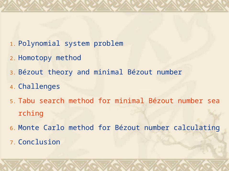
1. Polynomial system problem

2. Homotopy method

3. Bézout theory and minimal Bézout number

4. Problems

5. Tabu search method for minimal Bézout number searching

6. Monte Carlo method for Bézout number calculating

7. Conclusion


2. Homotopy method


4. Problems



7. Conclusion

1.1. Polynomial system problemPolynomial system problem

,,

)1.1(,

0),,(

0),,(

0),,(

:)(

1

1

12

11

n

nn

n

n

xxXwhere

xxp

xxp

xxp

XP

Mission: Find out all solutions of P(X).

Application: very common in many engineering fields

formula construction,

geometric intersection problems,

computation of equilibrium states,

etc.


2. Homotopy method


4. Problems



7. Conclusion

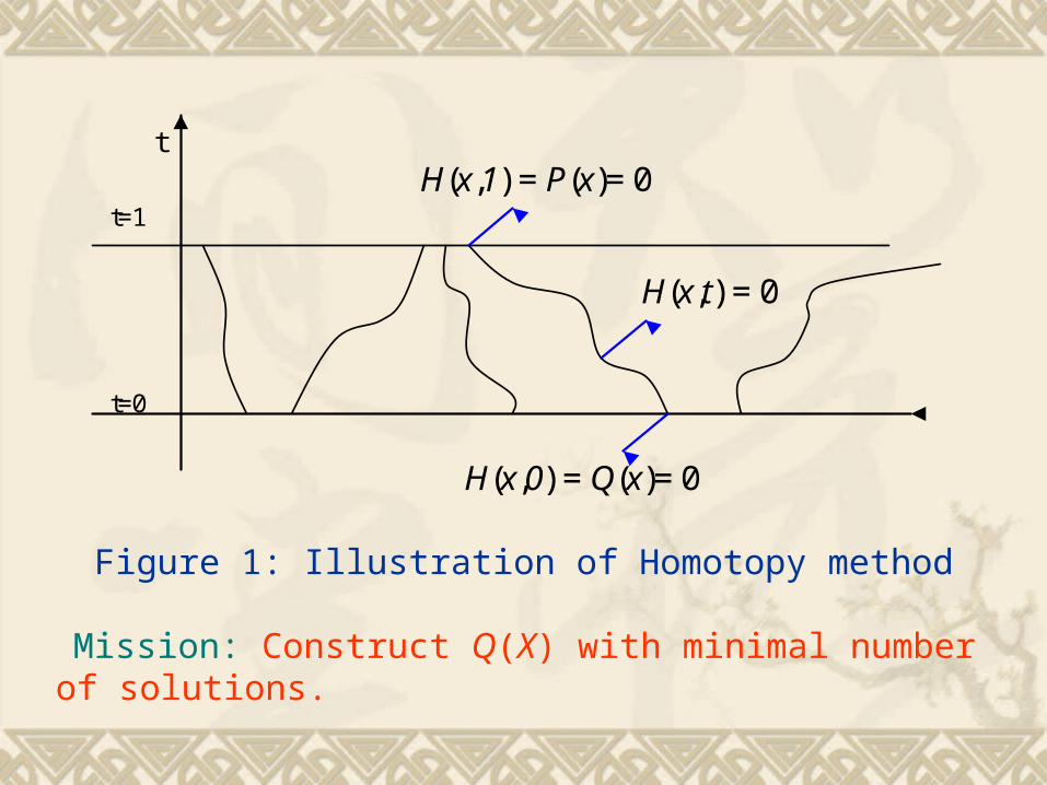
2.2. Homotopy methodHomotopy method

Homotopy Equation: )()()1(),( xtPxQttxH

Construct Q(x) that satisfy the conditions:

1. The solutions of Q(x) = 0 are either known or easy to known;

2. When 0≤t ≤1, the solutions of H(x,t) is consist of finite number of curves with parameter t;

3. Each solution of H(x, 1)= P(x) = 0 can be obtained by tracking curves starting from t = 0.

t

t=1

1111

1111

=

t=0

H(x,t) = 0

H(x,1) = P(x)= 0

H(x,0) = Q(x)= 0

Figure 1: Illustration of Homotopy method

Mission: Construct Q(X) with minimal number of solutions.


2. Homotopy method


4. Problems



7. Conclusion

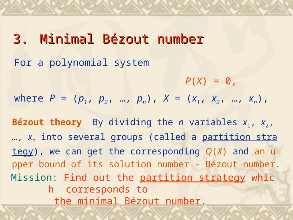
For a polynomial system

P(X) = 0,

where P = (p1, p2, …, pn), X = (x1, x2, …, xn),

Bézout theory By dividing the n variables x1, x2, …, xn into se

veral groups (called a partition strategy), we can get the corre

sponding Q(X) and an upper bound of its solution number - B

ézout number.

Mission: Find out the partition strategy which corresponds to the minimal Bézout number.

3.3. Minimal Bézout numberMinimal Bézout number

More detail ---

Divide X = (x1, x2, …, xn) into m groups:

X = (X (1), X(2), …,X(m)),

then we get

a) the degree matrix D = ( dij ), where dij is the degree of X (j) i

n Pi(X (1), X(2), …,X(m));

b) and partition vector K = (kj)T, where kj is the number of var

iables that X (j) contains.

Example 1:

( n = 3)

0

0

0

:)(2

321

32

232

1

2312

21

xxx

xxxx

xxxxx

XP

2

1

1

1

2

3

D

If X = (x1, x2, x3) is divide into 2 groups:

X = ( x1, x2 , x3 ), or ( 1, 2 , 3 ),

then we have

T1,2Kand

The formula for Bézout number B(D,K) is

nn

d

d

d

d

d

d

d

d

d

d

d

d

D

mk

nm

m

nm

m

k

nn

k

nn

11

2

12

2

12

1

11

1

11*

21

*

21 !!!

1),( DPer

kkkKDB

m

where

and Per(D*) is the permanent of matrix D*.

So, the Bézout number is

2

1

1

1

2

3

1

2

3*D

34!1!2

1),( * DPerKDB

where

2

1

1

1

2

3

D T1,2KandIn Example 1,


2. Homotopy method


4. Problems



7. Conclusion

Searching the optimal one in all possible partition strategies

Model: How many ways to put n balls into m (1≤m≤n ) boxes? The result is called the Bell number B(n), which has the following estimation

(n / 2) (n / 2) < B(n) < n!

4.4. ProblemsProblems

Computing Bézout number (or permanent)

The best-known algorithm is Ryser’s, O(n2n).


2. Homotopy method


4. Challenges



7. Conclusion

Main idea:

Construct neighbor relationship between partition str

ategies (or partitions), and apply Tabu (Taboo) searc

h method to search the optimal partition.

5.5. Tabu search method for minimal Bézout Tabu search method for minimal Bézout number searchingnumber searching

split: 1, 3, 6 5 2, 4

1, 3 6 5 2, 4

merge: 1, 3, 6 5 2, 4

1, 3 , 6 5, 2, 4

Two kinds of neighbor relationship

A partition has O(n2) neighbors.

Bézout number, right?

Evaluation function

But how can we calculate it ?

That’s our next problem.


2. Homotopy method


4. Challenges



7. Conclusion

Bézout number and permanent

)1.6()(!!!

1),( *

21

DPerkkk

KDBm

6.6. Monte Carlo method for Bézout number cMonte Carlo method for Bézout number calculatingalculating

Permanent

where A is an n×n matrix, and Sn is the set composed of all permutations of number 1, 2,…,n.

Example 2.

223452)(,54

32

APerA

)2.6()(,)(

nS

n

i iiaAPer

More about the permanent

The computation of permanents has been studied fairly extensively in algebraic complexity theory.

The complexity of the best-known algorithms grows as the exponent of the matrix size.

Application – Counting problems

The number of perfect matching -- 0-1 permanentThe number of Latin squares -- general permanent

We can see in the definition of permanent

a. any permutation of 1, 2,…,n, denoted byω, corresponds to one product term g(ω);

b. there’re totally n! product terms.

Let Sn be the sample space Ω. We have

Per(A) = θ· |Ω| = θ· n! (6.3)

whereθ= E(g(ω)) is the expectation of g(ω).

MC (Monte Carlo) Method

where

is the approximation of by sampling uniformly

from sample space Ω.

)4.6(!)( nAPer

)5.6(1

)(1

N

i

gN

Disadvantage of MC method

Too many zero-value product terms when matrix A i

s sparse, i.e., for an n×n matrix with sparsity p,

pn ≤ pn→0, n →∞

pn is the possibility of sampling a non-zero sample.

Applying simple Monte Carlo approach to our

problem is not very helpful.

Let

to be the sample space, then we have

where

Advantage |Ω+| << |Ω|

Question How to get and |Ω+ | ?

MC(Ω+) algorithm

)6.6()( APer

)7.6(1

)(1

N

i

gN

,0)(g

Let IA is a matrix that has the same structure as

A except that the non-zero entries is 1.

Obviously, we have

|Ω+ | = Per(IA)

Thus we can calculate |Ω+ | with 0-1 permanent

algorithms.

How to get |Ω+ | ?

The equivalent question is

How can we choose a How can we choose a non-zeronon-zero product term product term

uniformlyuniformly??

How to get or ? )( g

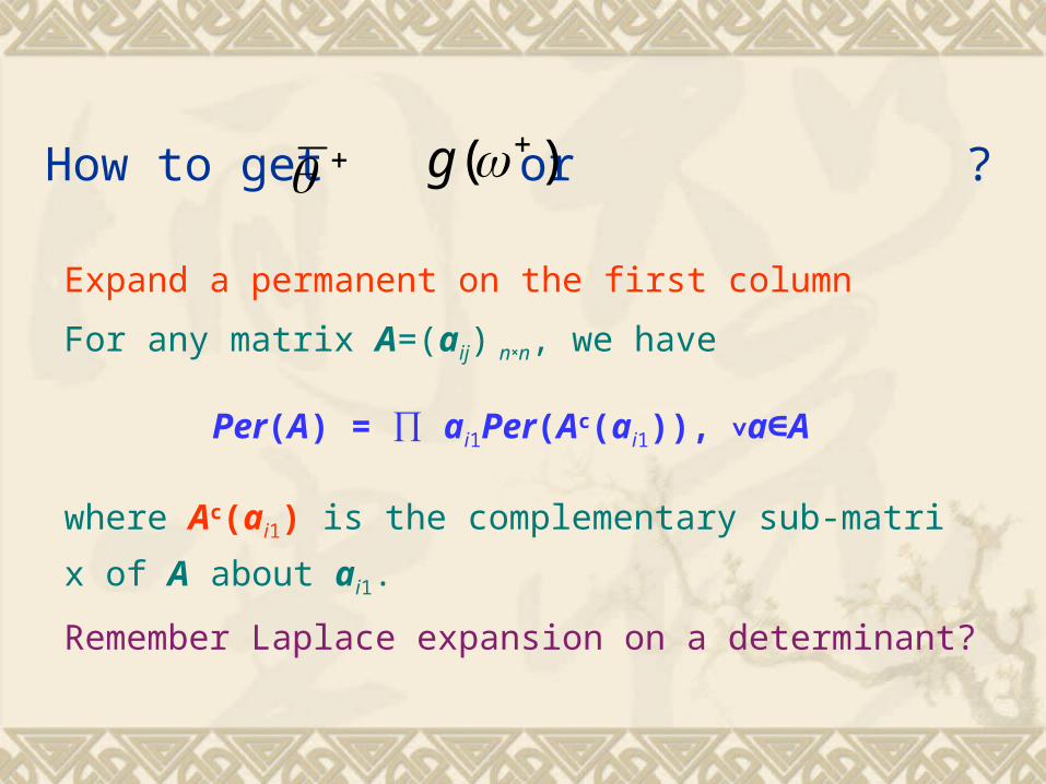
Expand a permanent on the first column

For any matrix A=(aij) n×n, we have

Per(A) = ∏ ai1Per(Ac(ai1)), ∨a∈A

where Ac(ai1) is the complementary sub-matrix of A a

bout ai1.

Remember Laplace expansion on a determinant?

How to get or ?)( g

Example,

5

0

1

1

4

6

0

2

3

A

then,

04

160

51

162

51

043)( PerPerPerAPer

Divide product terms into 3 groups!

How to get or ?)( g

↓ ↓ ↓ 1 product term 2 terms 0 term

04

160

51

162

51

043)( PerPerPerAPer

Choose “3” (group 1) with the probability 1/3,“2” (group 2) with 2/3, and “0” (group 3) with 0.

By iterating this procedure, we can finally sample uniformly a none-zero product term.

How to get or ?)( g

Layered MC(Ω+) algorithm

Basic Idea - Importance sampling

Divide the sample space Ω+ into several sub-spaces, in which the sample values are closer.

2 2

1 1

( ) ( ( )) ( )i

n nc

i i ii i

Per A a Per A a g

Ai – Keep the i largest entries of A, and others set to zero;

Ω+ is divided into n2 sub-spaces according to the value of product terms.

Product terms in sub-space are likely larger than those in sub-space .

)(Ai

1( )i A

Layered MC(Ω+) algorithm

How to assign sampling number to sub-spaces?

Based on

the dimension of sub-spaces;

the sums of product terms that have already been estimated in sub-spaces;

Lead to two algorithms: M1 and M2.

Numerical results

7.7. ConclusionConclusion

Polynomial systems

Homotopy method & Bézout theory

Searching for minimal Bézout number

Tabu search

Computing Bézout number

Monte Carlo method

Documents

Searching for the Minimal Bézout Number Lin Zhenjiang, Allen [email protected] Dept. of CSE, CUHK 3-Oct-2005 [email protected]