Embed Size (px)
Citation preview

Discussion(paper(2013112(
�
Search,(Project(Adoption(and(the(
Fear(of(Commitment(
(
(Vidya(Atal(Talia(Bar(
Sidartha(Gordon(
((((
Sciences(Po(Economics(Discussion(Papers(
Search, Project Adoption and the Fear of Commitment
Vidya Atal†, Talia Bar‡and Sidartha Gordon§
July 22, 2013
Abstract
We examine project adoption decisions of firms constrained in the number of projects
they can handle at once. Adoption requires a commitment for a period of uncertain du-
ration, restricting the firm in subsequent periods. Capacity constraints create a “fear
of commitment” — some positive return projects are not adopted. In the sequential
move dynamic game, the second mover sometimes adopts projects that were rejected
by the first, even when both firms are symmetric and equally informed. We study
the e§ects of competition on the fear of commitment, and compare the jointly optimal
adoption decision to the behavior of strategic non-cooperative firms.
We are grateful to Tal Cohen for insightful conversations and to Haim Bar for his detailed comments.
We also thank seminar participants at the 2011 International Industrial Organization Conference in Boston.†Department of Economics and Finance, Montclair State University. 1 Normal Avenue, Partridge Hall
427, Montclair, NJ 07043; email: [email protected].‡Department of Economics, University of Connecticut. 365 Fairfield Way, Oak Hall Room 309C, Storrs,
CT 06269; e-mail: [email protected].
§Department of Economics, Sciences Po, 28 rue des Saints-Pères, 75007 Paris, France; email:
1

Keywords: adoption, project selection, commitment, Markov perfect equilibrium
JEL Classification Codes: L10, L13, D21.
1 Introduction
Decision makers, such as researchers, firms and government agencies, often have to choose
whether to engage in projects that require committing limited resources. While resources are
committed to development or implementation of a project, they cannot be used in another
project; or a firm might need to put on hold its search for other projects. Projects may
include research, development or adoption of an invention, providing services to clients,
acquisition of an innovative start-up, and introduction of a new product to the market. Such
projects take time to complete, and tie a firm’s resources for a period of time. When making
a choice about a current project, the decision maker is typically not fully informed about
the duration of the commitment to the project or about future opportunities. Committing
limited resources (e.g., researchers’ and other employees’ time, physical space, lab equipment,
etc.) to one project may result in the need to forgo future, perhaps more profitable, projects.
In our infinite horizon model, new project opportunities arise every period. The decision
maker learns the expected return of the current period’s project, but is uncertain about
the return from future projects. We use dynamic programming to characterize the decision
maker’s adoption behavior. The optimal adoption policy is characterized by a reservation
value, so that a project is adopted if its expected return exceeds the reservation value.
Whereas unconstrained decision makers take on any project with a positive net expected
return, constrained decision makers are more prudent. They reject some projects that have
2
positive returns, so as not to commit resources and risk missing out on better opportunities in
the future. We refer to this tendency to wait for better projects as the “fear of commitment.”
The optimal reservation values will be higher (the decision maker will be more likely to reject
a current project) when each project commitment is expected to last longer, and when the
decision maker is more patient. The optimal adoption threshold is also higher when project
returns are drawn from a more favorable distribution, because there is a higher probability
that the return from a future project exceeds the return from the current project.
Repeated adoption decisions are often taken in competitive settings. Consider, for ex-
ample, the companies Coca-Cola and PepsiCo. While best known for their cola drinks, each
of these companies repeatedly adopted many innovative drinks. Coca-Cola company’s page
on Facebook, for example, states that the company has “a portfolio of more than 3,300
beverages, from diet and regular sparkling beverages to still beverages such as 100 percent
fruit juices and fruit drinks, waters, sports and energy drinks, teas and co§ees, and milk-and
soy-based beverages, our variety spans the globe.1” Adopting a product requires a period of
intense e§ort for the company. It involves conducting market research, designing the bottle
and label, developing a marketing strategy, etc.
The sports drink Gatorade was developed in 1965 in the University of Florida for its
football team the Gators.2 In 1992, after gaining increased popularity, Gatorade approached
Coca-Cola about using Coke’s distribution system.3 In 2000, after considering acquiring
Quaker Oats, the company that owned Gatorade, Coca-Cola decided against the acquisition.
As a headline in the Chicago Sun Times from November 22, 2000 states, “Coke backs o§ bid
1See https://www.facebook.com/pages/Coca-Cola-Cafe/173169246041187?sk=info2See http://www.gatorade.com/history/default.aspx3See http://www.time.com/time/magazine/article/0,9171,975619,00.html
3

to buy Quaker Oats - Company’s decision could open door for rival PepsiCo4,” in August
2001, PepsiCo acquired Quaker Oats for its Gatorade.
We study the optimal project adoption strategies of capacity constrained firms in a
dynamic duopoly game. Every period, one project opportunity arises. The expected return
from each period is randomly drawn from a known distribution. The first firm to consider
each project is selected at random. If it does not adopt the project, the other firm will
consider adopting it. When no commitment is required, the first firm to consider each project
adopts any project with a positive return, and the second firm never adopts a project that was
rejected by the first firm. But, when projects require commitment of resources for a certain
period of time, some positive return projects are not adopted by either firm. The first firm
will adopt projects that have a high enough return. Interestingly, there can be projects with
intermediate levels of return that are rejected by the first firm, yet adopted by the second
firm. This is true even though both firms are identical and have the same information
about project returns. The intuition for this result is that, for projects with intermediate
return, each firm prefers its rival to adopt the project, thus commit its resources leaving the
non-adopting firm with less competition over future, perhaps more profitable projects. This
result holds true whether the externality that the adopting firm imposes on the non-adopting
firm is positive or negative, provided that the magnitude of the externality is smaller than
the return from the project to the adopting firm.
To examine the e§ects of competition on the “fear of commitment,” we compare the
project adoption decisions of a firm who has no competition to that of a firm that faces a
strategic competitor. We find that adoption thresholds are lower under competition. That
4See http://www.highbeam.com/doc/1P2-4568251.html
4

is, a duopolist adopts projects that this firm would not have adopted absent a competitor
in the market.
We consider also the project adoption decisions of a firm that has a less strict capacity
constraint and can adopt two projects at a time. When a single firm decides on project
adoptions, we show that the less constrained firm has lower adoption thresholds (less fear of
commitment) than the more constrained firm. Interpreting the two-projects capacity model
as that of a joint venture of two firms with one project capacity each, we find that in duopoly
competition, firms exhibit more fear of commitment than in a joint venture.
The rest of this paper proceeds as follows. In Section 2, we discuss related literature. In
Section 3, we describe the basic model with a single decision maker. In Section 4, we develop
the game between duopolists and analyze the strategic interaction between them. Section
5 studies the single decision maker with two-projects capacity constraint and compares the
choices made in a joint venture to the choices made in the non-cooperative duopoly game.
Section 6 concludes.
2 Related Literature
Our model contributes to the literature on sequential search, and more specifically, to the
much smaller branch that studies the strategic interaction between a small number of search-
ing agents. We consider first the decision maker version of our model, and its relation to job
search models, and then describe the relation of our model to models of strategic search.
In our model, once a firm adopts a project, it commits resources to the development of
the project until its random termination date. In early job search models (e.g., McCall, 1970;
5

Mortensen, 1970), workers cannot search for a job while employed, and staying employed
is better than becoming unemployed. In recent years, Burdett and Mortensen (1998) and
Postel-Vinay and Robin (2002), have introduced models where workers continue searching
for a better job while employed. Thus in leading job search models, commitment is either
not binding or it is not assumed. In contrast, in our setting, the necessity to spend time and
other resources to developing the newly found projects is a natural source of commitment.
Binding commitments characterizes many situations firms face. For example, if a service
provider (e.g., a consulting firm) takes on a client, the firm is typically committed (legally or
to preserve his reputation) to complete the service promised; when adopting a project, firms
might enter binding agreements with its employees, clients, or suppliers; or, while working
on an existing project, the firms’ researchers might not observe new project opportunities.
Sometimes, at the start of a project, a large sunk investment is required which makes aban-
doning the project for another, even if it has a higher expected return, not worthwhile. In
labor search models, the worker alternates between spells of unemployment and employment.
Similarly, in our single firm model, the firm alternates between spells of search for a new
project and development of a project it recently found.
An important di§erence between our model and previous search models is that unlike
the job search case, the firm’s payo§ from a project is independent of the development
duration: one can interpret it as the present value of the project. The firm is stuck with
the development of a project until it is complete. Termination frees the firm to adopt an
additional profitable project without forgoing the returns of the earlier project. Whereas a
worker fears a layo§, our firm eagerly expects project completion. Being committed does
not allow the firm to engage in new project opportunities. This assumption is appealing for
6

the applications we consider. For example, if the firm needs to use its resources to develop a
new product that it will then market, the firm is better o§ when development is completed
and the product can enter the market. When the project terminates, the firm’s resources
are free and can be used for other projects, and it will still benefit from the product that
was developed and introduced to the market.
In our analysis of strategic interactions, our model also contributes to a sparse (but
highly relevant to the field of industrial organization) literature that studies search behavior
and project selection by strategic firms. Whereas the analysis of search and adoption by
single decision makers is important in competitive settings (such as in labor markets) or for
understanding monopolies, in many markets firms act strategically. A firm would take into
account how its own search and adoption strategies would a§ect the opportunities available
and the behavior of rivals. Our contribution to strategic search models lies in the form of
the strategic interaction between our searching firms, which di§ers from other interactions
that have been studied, and better applies to some strategic situations.
In the context of a game, in one category of models, known as patent or R&D races
(Loury 1979, Lee and Wilde 1980, Reinganum 1983b), search intensity is the main strategic
variable. In these models, there is essentially one object to be found, so that selectivity is not
an issue. The firms’ payo§s depend on which firm finds it first and how long the race lasts.
The main insight from these models is that, in equilibrium, firms search more intensively
than joint profit maximization would require.
In a surprisingly small second category of models, selectivity is taken as the main strate-
gic variable. Our model belongs to this group. In these models, firms play reservation
strategies, and a firm’s selectivity is therefore measured by the threshold it uses for adop-
7

tion.5 Reinganum (1982, 1983a) considers a game where sequential search for a technology
is undertaken simultaneously in a first stage. Firms do not observe the outcomes of the
other firms’ searches, but only their reservation thresholds. Once all firms have completed
their search, firms compete in the goods market. The dates at which the di§erent firms stop
searching and the order in which they complete the search play no role.6 Daughety and
Reinganum (2000) use a similar framework to study search for evidence by opposing parties
in a trial. Lippman and Mamer (1993) enrich Reinganum’s (1982) strategic search problem
by introducing a timing dimension. They assume an extreme form of first-mover advantage
whereby only the first adopter is rewarded. Hoppe (2000) extends the analysis to the case
where the loser of this race may benefit from second-mover advantages. Interestingly, a
firm’s best response threshold is nonincreasing in the other firm’s threshold in Reinganum
(1982), increasing in Lippman and Mamer (1993) and decreasing in Hoppe (2000) when the
second-mover advantage is strong enough. Our model di§ers from the ones discussed in this
paragraph in several important ways.
First, what all of these models have in common is that the agents search in di§erent
5Selectivity is also the decision variable in models of labor markets with many firms and workers, such as
Pissarides (1985). Firms’ and workers’ selectivity a§ect other agents through aggregate channels, but each
agent is infinitesimal and has no impact on any other agent. Also, because the rents of firm-worker matches
are independent across matches, being more selective has the same e§ect on other agents as searching less
intensively: it a§ects the hazard rate at which opportunities arrive, not the distribution of their flow value
conditional on arriving. In contrast, in our model, if one firm lowers its adoption threshold in some period
(it is less selective), the distribution faced by the other firm in the same period is modified.6Taylor (1995) examines the planner’s optimal design problem of a search tournament: the planner chooses
the number of competing firms, the entry fee and the prize. The firms then engage in simultaneous search
as in Reinganum (1982, 1983a). The firm that finds the best innovation receives the prize.
8

pools. The interaction comes from the e§ect that the other agent’s search outcome has in a
subsequent stage (competition on a goods market, trial, etc.) The value of what an agent
finds depends on what the other agents find. However, what an agent can find does not
depend on the other agent’s behavior. In contrast, in our model, the selectivity of a firm
at any point in time a§ects the distribution of projects faced by the other firm both in the
same period and in subsequent periods in complicated ways. If firm 1 is approached first by
an innovator in some period, and adopts his project, then on the one hand firm 2 will not
receive any o§er in the same period. But on the other hand, firm 1 might be committed for
a certain period of time, which will leave firm 2 as a temporary monopolist in the market for
innovation until either firm 1 completes developing its product or firm 2 adopts a project.
The second di§erence is that, in our model, what each firm has found and adopted is common
knowledge. Firms best respond not only to the other firm’s thresholds strategies, but also
to their current state. The third di§erence is that our firms alternate between periods of
search and periods of development. This is a common setting in job search models, but, to
the best of our knowledge, it has not been analyzed in a strategic search game.
In its application, our work relates to a literature in management and finance on capital
allocation. This literature considers mostly the decision to finance a single project, and much
of the work focuses on information asymmetry (see, for example, Harris and Raviv, 1996 and
Zhang, 1997). In our paper, information is symmetric, and the focus is on the need to commit
limited capacity. Hall and Lerner (2010) survey the literature on financing of innovation with
a focus on financial market reasons for under-investment. Our assumption on firms’ project
capacity constraint is di§erent from the standard capital financing constraint. It is not
enough for firms to be able to borrow at a reasonable interest rate. Firms can be limited
9
in the number of projects they adopt even if they have cash reserves, or access to venture
capital. Capacity constraints could arise due to a limited number of skilled scientists and
engineers, limited physical space to run experiments, etc. The problem our paper analyzes
has also some similarity to the problem of dynamic assignment of a single durable object to
successive agents, considered by Bloch and Houy (2011). In their model, the firm prefers to
learn an agent’s type before assigning him an object. In our model, the type of the project
is known and the project immediately dies if it is not adopted. Our focus is on the e§ect of
competition and capacity constraints on the fear of commitment.
3 Basic Model
We begin by describing the model in the context of one decision maker — a single firm
repeatedly deciding whether to adopt projects that arise sequentially. In the next section,
we add strategic interactions between firms.
Consider a discrete time infinite horizon model. The decision maker maximizes the
discounted sum of expected payo§s. The discount factor is 0 < < 1. A new project
opportunity arises every period. If the decision maker is not yet committed, he can decide
whether to adopt the project. A project requires a commitment of resources, which prevents
the firm from engaging in another project at the same time. The duration of a project is
random. To capture this, we assume that every period, conditional on being committed
in the previous period, the commitment ends with a probability p. The decision-maker has
resource constraints so that he can be committed to only one project at a time. Hence,
the decision maker can only adopt a project if he is not currently committed to an earlier
10
project. If we think of a project as the acquisition of a start-up innovative firm, the duration
of the commitment can include the time it takes to transfer knowledge from the innovator
to the firm, time to develop the product, time to come up with a marketing strategy, etc.
A project’s return v is the expected discounted present value of benefits from the project
at the time it is adopted.7 Project returns are identically and independently drawn from
a known distribution. The cumulative distribution function for project returns is F (v) on
[v, v], with v 0, and a finite v > 0. For all v > 0, we assume F is di§erentiable with a
finite density f(v) > 0. There may be an atom (a discontinuity in F ) at zero, so as to allow
for a positive probability that no project arises. The payo§ in a period in which no project
is adopted is zero.
3.1 A Single Decision Maker’s Adoption Behavior
Let us denote the value function in any period for which the decision maker is not com-
mitted, before realization of the project’s return, by V0. Let V1 denote the value function
for the decision maker who is committed from an earlier period. If the decision maker is
not committed, then when a project has a payo§ of v, adopting a project has a payo§
v + (pV0 + (1 p)V1) and not adopting the project has a payo§ V0. The decision maker
maximizes payo§ by choosing to adopt or not to adopt:
max
8<
:v + (pV0 + (1 p)V1)| {z }adopt
, V0|{z}don’t adopt
9=
; .
7The assumption that the prize is obtained immediately simplifies the exposition, but the analysis will
be similar if the prize is obtained at the end of the commitment period.
11

The project is adopted if v+ (pV0 + (1 p)V1) V0. This decision rule defines a threshold
for adoption:
v0 = (1 p) (V0 V1) . (1)
The value in the state without commitment is:
V0 =
v0Z
v
V0f(v)dv +
vZ
v0
[v + (pV0 + (1 p)V1)] f(v)dv
= V0 +
vZ
v0
(v v0) f(v)dv. (2)
The value in the committed state is:
V1 = [pV0 + (1 p)V1] .
Re-arranging, we have:
V1 =p
1 (1 p)V0. (3)
Substituting (3) into (1) and then into (2), and re-arranging, we obtain the following implicit
definition of the adoption decision threshold v0:
1 (1 p) (1 p)
v0 =
vZ
v0
(v v0) f(v)dv. (4)
Lemma 1 There exists a unique solution to (4) in the range (0, v) which defines the adoption
threshold.
Lemma 1 implies that an optimal threshold return exists and is unique. Unless p = 1,
this threshold is strictly positive, that is, when the decision maker can only commit to one
project at a time and a project’s expected duration is longer than one period, some positive
return projects are not adopted.
12

The next proposition presents comparative statics results describing how the reservation
value depends on the parameters and p.
Proposition 1 The reservation value v0 is lower the more likely is the project to end (the
higher p), i.e., the shorter is the expected commitment time and the more patient the decision
maker is (the higher ).
The proposition is proved by implicit di§erentiation of (4). Intuitively, the threshold is
higher when the commitment required for each project is expected to last longer, because
adopting the project is more costly in terms of missed future opportunities. In the phar-
maceutical industry, for example, where it takes about 10 years to bring a drug to market
(see Nicholas, 1994), we would expect higher adoption thresholds than in areas with short
duration projects, as perhaps is true in the context of software development. Conditional on
the project being adopted, project return is expected to be higher in an industry in which
project duration is longer.
The adoption threshold is also higher when the decision maker is more patient. This is
because waiting for a potentially better project in the future is less costly to him. Combining
the results for and p, we also conclude that if project opportunities arise more frequently,
then the project adoption reservation value would be higher. This is because in a setting
with more frequent project opportunities, the discount factor is higher (as there would be
a lower discount rate per shorter period) and there is a smaller probability that the project
terminates by the following period. Comparing a decision maker (or firm) that is more
prolific or creative and can generate frequent projects to a less prolific one, we would expect
the more prolific decision maker to adopt higher return projects.
13

We next compare the thresholds of adoption for two distributions of project returns, one
of which is either more favorable in terms of first order stochastic dominance, or a mean
preserving spread of the other. In the first case, the threshold for adoption is higher for the
dominating distribution, because there is a higher probability that a better project will arise
in the following periods. In the second case, the threshold for adoption is higher for the
spread, because the option value of waiting for a better project is higher, under the riskier
distribution.
Proposition 2 For a distribution of returns that either first order stochastically dominates
another one or is a mean-preserving spread of another one or if both of these statements
hold, the threshold level is at least as high.8
In research areas where projects tend to have higher values, decision makers will be less
likely to commit to projects of relatively lower value. Similarly, in research areas where
projects have the same expected values but more risky returns, decision makers will be less
likely to commit to projects of relatively lower value, because the option value of waiting for
a better project is higher.
4 Strategic Decision Makers
In this section, we examine the project adoption decisions in a duopoly setting. One firm’s
adoption decision can a§ect the payo§s of the other. We assume only one firm can adopt
8Equivalently, for any two cumulative distributions F 0 and F 1 such that any weakly increasing and convex
utility function u over returns we haveRu (v) dF 0
Ru (v) dF 1, the threshold level is higher under F 1 than
under F 0.
14
each project. We examine project adoption strategies and the e§ects of competition on the
fear of commitment.
4.1 The Game
We consider competition between two firms A and B. Every period, a new project oppor-
tunity with a value v drawn from the distribution F (v) arises. One firm chosen at random
(each firm is chosen with a probability 12) is the first to make a decision to adopt the project
or not. If the first firm adopts the project, the period ends. If the first firm does not adopt
the project, the other firm can decide whether to adopt it. As we assumed before, a firm
can adopt at most one project at a time and the commitment of resources ends each period
with a probability p. The adopting firm obtains rights to a patent, or a lead time advantage
resulting in the random return v. For a project with return v to the adopting firm, we denote
the return of the non-adopting firm by v, where 2 (1, 1) . When < 0, a firm su§ers a
negative externality if its rival adopts the project. This can be the case for example if the
project results in an improvement of quality or reduction in cost for the adopting firm, which
reduces profits and market share for the non-adopting firm. When > 0, a firm enjoys a
positive externality if the other firm adopts the project. A firm can benefit from its rival’s
adoption when there are network externalities, or technology spillover. The non-adopting
firm can also benefit if, for example, the project involves the introduction of a new product,
and the first adopting firm becomes a Stackelberg leader in the product market, while the
non-adopting firm becomes a follower. Either way, we assume the return for the rival firm
is smaller in magnitude than the return for the adopting firm, || < 1. If no firm adopts the
15

project, payo§s are zero for each firm.
We restrict attention to Markov strategies. A firm’s decision will only depend on the
current state. States of the world are denoted by (i, j), where i, j 2 {0, 1}. In a state with
i = 0 firm A is not committed and in a state with i = 1 firm A is committed. Similarly, j
indicates the commitment of firm B.
We look for a symmetric Markov perfect equilibrium. The value function (before realiza-
tion of the project’s return and the choice of the first mover) in any state (i, j) is denoted by
V Ai,j for firm A and VBi,j for firm B. Because we focus on symmetric equilibria, V
Ai,j = V
Bj,i = Vi,j.
Equilibrium strategies are characterized by threshold levels of return. The threshold for the
non-committed firm in a state (0, 1) is denoted by v0,1. In state (0, 0) , the threshold for the
firm that was o§ered the project first is v10,0 and for the second firm (in case the first firm
rejected the project), we denote the threshold by v20,0.
4.2 Analysis
In state (1, 1) , both firms are committed and no firm can adopt a project. Next period’s
state depends on whether each of the firms is freed from its previous commitment or not.
The value in state (1, 1) is thus given by:
V1,1 = p2V0,0 + p (1 p)V1,0 + p (1 p)V0,1 + (1 p)
2 V1,1. (5)
In state (0, 1), firm B is committed and it cannot adopt a project. Hence, if firm A does
not adopt, no firm adopts. If a project with return v arises, firm A can either adopt it and
immediately transition to the state (1, 1) where both firms are committed, or not adopt and
transition in the next period to one of the states where it is not committed. Hence, firm A
16

will maximize:
max
8><
>:v + V1,1| {z }adopt
, (pV0,0 + (1 p)V0,1)| {z }don’t adopt
9>=
>;.
The threshold return for adoption is:
v0,1 = (pV0,0 + (1 p)V0,1) V1,1. (6)
Accounting for these thresholds of adoption for the non-committed firm, the value functions
in states (0, 1) and (1, 0) are:
V0,1 =
vZ
v0,1
vf (v) dv + (1 F (v0,1))V1,1 + F (v0,1) (pV0,0 + (1 p)V0,1) , (7)
V1,0 =
vZ
v0,1
vf (v) dv + (1 F (v0,1))V1,1 + F (v0,1) (pV0,0 + (1 p)V1,0) . (8)
In state (0, 0), one of the firms is chosen at random to consider the project first. If the
first firm does not adopt the project, then the second firm faces the choice:
max
8><
>:v + (pV0,0 + (1 p)V1,0)| {z }
adopt
, V0,0|{z}don’t adopt
9>=
>;.
The threshold level is:
v20,0 = (1 p) (V0,0 V1,0) . (9)
Returning to the first firm’s decision, if v v20,0 so that the second firm will adopt if it has
the opportunity to do so, then the first firm faces the choice:
max
8><
>:v + (pV0,0 + (1 p)V1,0)| {z }
adopt
, v + (pV0,0 + (1 p)V0,1)| {z }don’t adopt ) rival adopts
9>=
>;.
The firm would adopt this project if the following condition holds:
v (1 p)(1 )
(V0,1 V1,0) := ev.
17

If v < v20,0 so that the second firm will not adopt the project even if the first firm to consider
it did not, then the first firm faces essentially the same choice as that of the second firm
after the first firm rejected a project. Because we are considering the range v < v20,0, the first
firm does not adopt such project. Thus, for v < v20,0, neither firm adopts. The threshold of
adoption for the first firm is therefore:
v10,0 = maxv20,0, ev
v20,0. (10)
For v v10,0, the first firm adopts. If (V0,0 V1,0) < 1(1) (V0,1 V1,0) , then there is a range
of project returns v20,0 v < v10,0 so that the first firm to be o§ered the project does not
adopt, but the second firm does. The equation that defines the value function in state (0, 0)
is given by:
V0,0 =
vZ
v20,0
(1 + )
2vf (v) dv + F
v20,0V0,0 +
1 F
v20,0 (1 p) (V0,1 + V1,0) + 2pV0,0
2.
(11)
In the special case where p = 1, each project only lasts one period. The commitment of
resources is not a binding constraint. It follows immediately from the system of equations
above that the thresholds of adoption satisfy v20,0 = v0,1 = v10,0 = 0. That is, when p = 1, a
firm will adopt any project that has a positive expected return. From now on, we consider
p < 1, when commitment is necessary.
Proposition 3 For p < 1, in a symmetric Markov perfect equilibrium, the thresholds for
adoption in state (0, 0) satisfy v10,0 > v20,0, so that in the range v
10,0 > v v20,0, the first firm
rejects the project, but the second firm adopts it. Additionally, v10,0 v0,1, (with a strict
inequality for p > 0), so that a firm is more selective when its rival is not committed.
18

From (10) , we know that v10,0 v20,0. This means that the first firm to be o§ered a project
never accepts one that would have been rejected by the second firm. When project returns
are low, v < v20,0, the project is not adopted. When project returns are high, v v10,0 the first
firm to be o§ered the project accepts it. Interestingly, Proposition 3 implies that there are
intermediate values of project returns for which the first firm to be o§ered the project passes
on the opportunity. Yet, the second firm who is o§ered the same project, adopts it. These
intermediate range project returns are high enough for the second firm to adopt, (knowing
that its rival already decided not to adopt the project), but not high enough to induce the
first firm to adopt. This is because the first firm knows that if it does not adopt the project,
its rival will adopt it, committing resources and leaving the first firm in a better position to
adopt projects in future periods.
To examine the e§ects of competition on the fear of commitment, we compare the adop-
tion rates when two firms compete to those of the single decision maker. We show that the
threshold return for a project to be adopted is lower when two firms compete than when
there is a single decision maker. Thus, competition reduces the fear of commitment.
Proposition 4 Competition reduces the fear of commitment: v10,0 < v0.
The comparison in Proposition 4 is done under the assumption that the project return
has the same distribution in the single decision maker’s problem and in the game. If the firm
enjoys a higher return from any project when it is alone in the market, the distribution of
returns in the decision maker’s problem may dominate that in the duopoly case. As we have
shown in Proposition 2, this would imply an even higher threshold of adoption. So the result
of Proposition 4 holds even if the decision maker earns more from each project compared to
19
the duopolist.
5 Two Projects Capacity Constraint
We consider now a single decision maker’s project adoption rule when the decision maker
has enough resources to work on two, but not more, projects at the same time. We compare
the decision maker’s choice in the two projects capacity model to the single project capacity
constraint. Also, this version of the model allows us to compare project adoption decisions
of strategic non-cooperative firms with the decision of a joint venture. We first set up
the dynamic programming equations for the (single decision maker) two projects capacity
case. We assume that when a project of value w arises, its adoption results in a payo§ of
w (1 + ) to the decision maker. This payo§ is the sum of payo§s in the game we solved
in the previous section. We can then compare the equilibrium project adoption behavior
to the optimal adoption behavior of the joint venture. We think of this joint venture as
a coordinated adoption decision of the projects, but no collaboration among firms in the
product market. We also consider the special case = 0 which can be interpreted as the
optimal decision for a single decision maker with two-projects capacity. Examining this case
allows us to compare the adoption thresholds of a single decision maker with one or two
projects capacity.
We denote the value functions of the decision maker with two projects capacity with
Wi, to distinguish from that of single project capacity values Vi. The index in the value Wi
refers to the number of projects to which the decision maker is committed, i 2 {0, 1, 2} . In
state 2, when committed to two projects, the decision maker cannot adopt a project. The
20
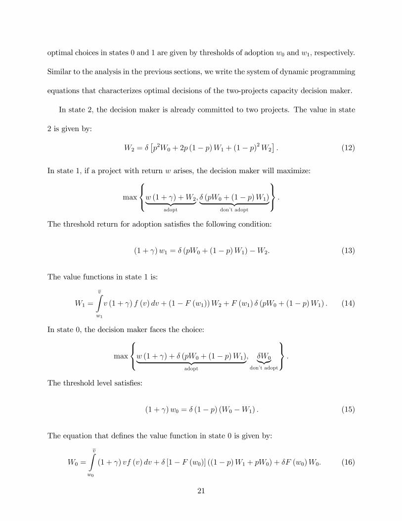
optimal choices in states 0 and 1 are given by thresholds of adoption w0 and w1, respectively.
Similar to the analysis in the previous sections, we write the system of dynamic programming
equations that characterizes optimal decisions of the two-projects capacity decision maker.
In state 2, the decision maker is already committed to two projects. The value in state
2 is given by:
W2 = p2W0 + 2p (1 p)W1 + (1 p)
2W2
. (12)
In state 1, if a project with return w arises, the decision maker will maximize:
max
8<
:w (1 + ) +W2| {z }adopt
, (pW0 + (1 p)W1)| {z }don’t adopt
9=
; .
The threshold return for adoption satisfies the following condition:
(1 + )w1 = (pW0 + (1 p)W1)W2. (13)
The value functions in state 1 is:
W1 =
vZ
w1
v (1 + ) f (v) dv + (1 F (w1))W2 + F (w1) (pW0 + (1 p)W1) . (14)
In state 0, the decision maker faces the choice:
max
8<
:w (1 + ) + (pW0 + (1 p)W1)| {z }adopt
, W0|{z}don’t adopt
9=
; .
The threshold level satisfies:
(1 + )w0 = (1 p) (W0 W1) . (15)
The equation that defines the value function in state 0 is given by:
W0 =
vZ
w0
(1 + ) vf (v) dv + [1 F (w0)] ((1 p)W1 + pW0) + F (w0)W0. (16)
21

Equations (12)-(16) define the solution to the optimal decision of the firm who can adopt at
most two projects.
We reduce the system to a system of two equations in only the thresholds w0 and w1.
We first show that the decision maker is less likely to adopt a project when she has already
committed resources to one project, i.e., w1 > w0.
Proposition 5 For a decision maker who can commit to adopt at most two projects, the
fear of commitment is greater when one project is underway than when it is not committed,
w1 > w0.
This result is intuitive, if the firm has not yet adopted any project, adopting the current
project will tie resources but still leave an opportunity to adopt another promising project
in the next period. However, for a firm that is already committed, adopting now means that
it cannot adopt until the commitment to one of the projects ends.9
In the next two subsections, we use the system derived above to examine how the decisions
of firms with di§erent capacity constraints compare (the case = 0), and also how the
adoption decisions of strategic players compare to that of a joint venture.
5.1 Adoption Decision and Project Capacity Constraint
We compare the adoption strategy of a firm that has only one project capacity to that
of a less constrained firm that has a 2-projects capacity. In Section 3.1, we derived the9Interestingly, the inequality w1 > w0 remains true in the limit where firms are infinitely patient ( ! 1),
when the firm is assumed to maximizes the expected payo§ per unit of time. The firm prefers to spend more
time in states 0 and 1 than in state 2 (where it is committed and cannot accept projects). Setting w1 > w0
is a way to steer the system back towards state 0, as it gets closer to state 2.
22
adoption threshold v0 of the single project capacity firm. The analysis in the beginning of
this section, when specialized to the case = 0, describes the adoption thresholds w1 and w0,
that a 2-projects capacity decision maker has when he is committed to one project, or when
he is not committed to any project, respectively. Our next proposition establishes that the
single project decision maker has a higher threshold of adoption compared to the threshold of
adoption of the 2-projects capacity firm, even when this firm has already committed resources
to one project. Intuitively, the reason for this is that for the two projects capacity firm, when
all its resources are committed, the expected time until at least one of the commitments is
relieved is shorter than for the single project capacity firm who has committed all of its
resources as the probability that one of two projects ends is larger than the probability that
one project ends.
Proposition 6 For a decision maker who has a capacity of one project, the fear of com-
mitment is greater than for a firm with two projects capacity, even when the two projects
capacity firm has already committed resources to one project, i.e., v0 > w1.
An implication of Proposition 6 is that the average return of adopted projects is larger for
a firm that has a more stringent project capacity constraint, because the fear of commitment
leads the constrained firm not to adopt some relatively low return projects that the less
constrained firm would adopt.
5.2 Joint Decision versus the Non-cooperative Game
The analysis in this section accounts for the payo§ externality parameter, 2 (1, 1) , as
in the game analyzed in Section 4. It allows us to compare the adoption strategies of firms
23
in the non-cooperative game to the behavior of a decision maker that jointly decides on the
adoption rule of both firms. This joint decision maker has a 2-projects capacity. There are
two comparisons of interest. First, we compare w1 to v0,1. That is, we compare the adoption
threshold of the 2-projects capacity firm when it is committed to one project but is free to
adopt another to the adoption threshold of a firm that is not committed but has a rival that
is committed. Second, we compare w0 to v20,0. That is, we compare the threshold of the
2-projects capacity firm when it is free of commitments, to the adoption threshold above
which at least one of the competing firms in the game adopts when both firms are free of
commitment.
Proposition 7 A non-cooperatively competing duopolist has a stronger fear of commitment
(higher thresholds of adoption) compared to the jointly optimal decision maker, w1 < v0,1
and w0 < v20,0.
To prove this proposition, we first argue that the joint decision maker can obtain at least
as high a value in state 0 as the sum of values of both firms in the game in state (0, 0) ,
i.e., W0 2V0,0. This is true because the decision maker can mimic the adoption strategies
in the equilibrium of the game. We then derive the given inequalities on thresholds from
the systems of dynamic programming equations. Proposition 7 suggests that competition
between firms with capacity constraints on project adoptions results in firms setting too
high a bar for adoption, compared to what would be optimal for them under a joint decision
making.
24

6 Concluding Remarks
Project adoption often requires firms to commit limited resources, preventing them from
adopting other projects while they are committed. Because more promising projects could
arise during the time a firm is committed to a project it adopted earlier, constrained firms
have a tendency not to adopt some profitable projects. We referred to this phenomenon as
a “fear of commitment.”
We first considered a single decision maker that could adopt at most one project at a
time. We characterized conditions under which the fear of commitment was stronger. The
constrained firm has a reservation value such that it adopts only projects that exceed this
value. The reservation value is higher when project commitment is expected to be longer,
when the firm is more patient, and if project opportunities arise more frequently. As a result,
in industries with long project durations, like the pharmaceutical industry, the expected
return from adopted projects would be higher compared to industries where projects do not
require long commitments. Also, a more prolific firm (that has frequent potential projects)
would adopt higher return projects. The reservation value is also higher for firms that face
a first order stochastically dominating distribution of project returns.
We compared firms with di§erent project capacities. Compared to a firm with one project
capacity, a less constrained, two-projects capacity firm has less fear of commitment even
during a period when it is already committed to one project and has resources available only
for one other project.
In a strategic environment, project adoption by one firm can change the profitability of
a rival, as well as the rival’s opportunity to adopt. Not adopting a project allows a rival
25

to adopt it, while adopting a project will increase the rival’s opportunity to adopt future
projects. We show that firms sometimes prefer their rivals to adopt a project, so as to lessen
future competition on projects. Our analysis suggests that there is a range of project returns
for which the first firm to consider the project does not adopt it, but the second firm does.
This may explain why we sometimes observe firms adopting projects that rivals, who had
an opportunity to adopt before, did not.
Our analysis suggests that firms that face a strategic rival will tend to adopt projects of
lower expected value than firm who do not face competition: competition reduces the fear of
commitment. But had the firms been able to jointly make adoption decisions, their adoption
thresholds would have been lower than in the non-cooperative equilibrium.
In attempt to maintain tractability and a simple exposition, we made certain simplifying
assumptions. In our model, if the firm is committed to a project, it cannot adopt another
project until the commitment ends. In reality, it is likely that firms can at some cost be
released from a previous commitment. Another way to look at this is to think of the firm
making a fixed sunk investment every time it adopts a project. This cost needs to be incurred
again if the firm switches to another project. We analyzed the case in which these fixed costs
are high. More generally, when the fixed cost is not too high, if a new project of high enough
return arises, the firm might find it worthwhile to abandon an old project and adopt the new.
Thus, firms also have thresholds of adoption in states where their resources have already been
committed. Assuming it is su¢ciently costly to be released from a previous commitment,
the fear of commitment would still be present, and we expect the results to be qualitatively
similar.
In analyzing strategic interactions, our model assumes sequential decisions. One can make
26
alternative assumptions on the nature of the game. For example, firms might simultaneously
decide on project adoption, or one firm might be a leading firm and always have the first
opportunity to decide on adoption, or the order of sequential move might be endogenous as
well. We expect that some of our results will carry over to such variations of the model,
but others will not. In particular, our result in Proposition 3 that the first firm may reject
projects that the second firm adopts, obviously relies on the sequential play assumption.
Instead, in the simultaneous game, in a symmetric equilibrium, there may be a range of
intermediate project returns for which firms randomize the decision to adopt.
We considered the strategic behavior of the adopting firms, but not of projects. If,
however, project opportunities arise when independent innovators propose them, they might
also act strategically so as to extract surplus from the adopting firms. The game played each
period might take the form of an auction or a bargaining game in such circumstances. These
extensions might be interesting to pursue in future work.
A Appendix: Proofs
Proof of Lemma 1. From (4) , we know that v0 is the solution to g(x) = 0 where g(.)
takes the following form:
g(x) =[1 (1 p)] (1 p)
xvZ
x
(v x) f(v)dv. (17)
Evaluating g(x) at x = 0 and at x = v, we find that:
g(0) < 0 and g(v) > 0.
27
Therefore a solution exists. Now, di§erentiating the function g (x), we find that:
g0 (x) =[1 (1 p)] (1 p)
+ [1 F (x)] > 0.
This implies that there exists a unique solution to (17) in the range (0, v).
Proof of Proposition 1. Consider g(v0, , p) as defined in (4) only taking into account
the parameters and p as arguments of the function. Implicit di§erentiation of g(v0, , p) = 0
shows that:
@g
@v0
dv0dp
+@g
@p= 0)
dv0dp
= @g
@p/@g
@v0,
@g
@v0
dv0d
+@g
@= 0)
dv0d
= @g
@/@g
@v0.
From the proof of Lemma 1, we know that @g@v0> 0. Hence,
sign
dv0dp
= sign
@g
@p
= sign
v0
(1 p)2
< 0.
We conclude that the reservation value is lower the higher the probability that the project
ends, or the shorter is the expected time the decision maker will be committed when taking
on a project.
Similarly,
sign
dv0d
= sign
@g
@
= sign
v0
2 (1 p)
> 0.
Thus, the reservation value is higher the more patient the decision maker is.
Proof of Proposition 2. The threshold return level solves g(v0) = 0 which we defined
in (17) in the proof of Lemma 1. Using integration by parts, we rearrange the function g
28
and write it as:
g (v0) =[1 (1 p)] (1 p)
v0 vZ
v0
[1 F (v)] dv. (18)
Consider two cumulative distribution functions F a and F b, defined on the interval (1,+1) ,
which contains their compact supports [va, va] and [vb, vb]. For all v < vi, let F i (v) = 0 and
for all v > vi, let F i (v) = 1. Let ga (v) and gb (v) be defined on (1,+1) as in (18) for the
corresponding distribution F a or F b. From Lemma 1, we know that these functions are both
increasing in v. Denote va0 and vb0 the solutions to ga (v) = 0 and gb (v) = 0, respectively.
First, consider the case where F b first order stochastically dominates F a, i.e., F b (v)
F a (v) for all v 2 (1,+1) , with a strict inequality for at least some v. Then gb (v) ga (v)
for all v, with a strict inequality for some v. In particular, gb (va0) ga (va0) = 0. Because
the function gb is increasing, this implies that va0 vb0, which is the desired conclusion. Note
that if the inequality F b (v) F a (v) is strict for some v > va0 , we obtain a strict inequality
va0 < vb0. If F
b (v) = F a (v) for all v > va0 , then va0 = v
b0.
Second, consider the case where F b is a mean preserving spread of F a, i.e.
vZ
1
F b (v) F a (v)
dv 0 (19)
for all v (with a strict inequality for some v) and
+1Z
1
F b (v) F a (v)
dv = 0. (20)
29
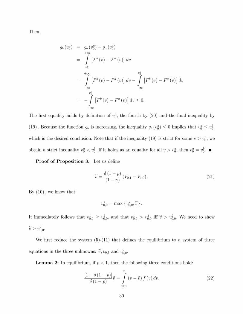
Then,
gb (va0) = gb (v
a0) ga (v
a0)
=
+1Z
va0
F b (v) F a (v)
dv
=
+1Z
1
F b (v) F a (v)
dv
va0Z
1
F b (v) F a (v)
dv
=
va0Z
1
F b (v) F a (v)
dv 0.
The first equality holds by definition of va0 , the fourth by (20) and the final inequality by
(19) . Because the function gb is increasing, the inequality gb (va0) 0 implies that va0 vb0,
which is the desired conclusion. Note that if the inequality (19) is strict for some v > va0 , we
obtain a strict inequality va0 < vb0. If it holds as an equality for all v > v
a0 , then v
a0 = v
b0.
Proof of Proposition 3. Let us define
ev = (1 p)(1 )
(V0,1 V1,0) . (21)
By (10) , we know that:
v10,0 = maxv20,0, ev
.
It immediately follows that v10,0 v20,0, and that v10,0 > v20,0 i§ ev > v20,0. We need to show
ev > v20,0.
We first reduce the system (5)-(11) that defines the equilibrium to a system of three
equations in the three unknowns: ev, v0,1 and v20,0.
Lemma 2: In equilibrium, if p < 1, then the following three conditions hold:
[1 (1 p)] (1 p)
ev =vZ
v0,1
(v ev) f (v) dv. (22)
30
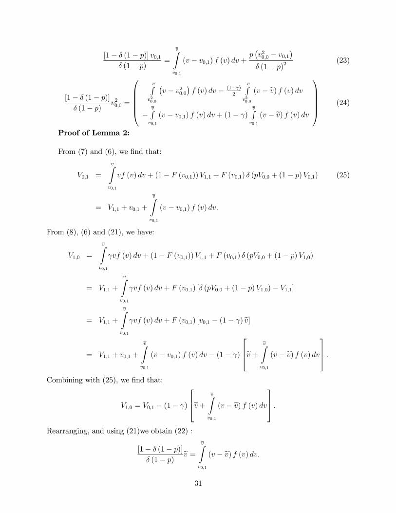
[1 (1 p)] v0,1 (1 p)
=
vZ
v0,1
(v v0,1) f (v) dv +pv20,0 v0,1
(1 p)2(23)
[1 (1 p)] (1 p)
v20,0 =
0
BBBB@
vR
v20,0
v v20,0
f (v) dv (1)
2
vR
v20,0
(v ev) f (v) dv
vRv0,1
(v v0,1) f (v) dv + (1 )vRv0,1
(v ev) f (v) dv
1
CCCCA(24)
Proof of Lemma 2:
From (7) and (6), we find that:
V0,1 =
vZ
v0,1
vf (v) dv + (1 F (v0,1))V1,1 + F (v0,1) (pV0,0 + (1 p)V0,1) (25)
= V1,1 + v0,1 +
vZ
v0,1
(v v0,1) f (v) dv.
From (8), (6) and (21), we have:
V1,0 =
vZ
v0,1
vf (v) dv + (1 F (v0,1))V1,1 + F (v0,1) (pV0,0 + (1 p)V1,0)
= V1,1 +
vZ
v0,1
vf (v) dv + F (v0,1) [ (pV0,0 + (1 p)V1,0) V1,1]
= V1,1 +
vZ
v0,1
vf (v) dv + F (v0,1) [v0,1 (1 ) ev]
= V1,1 + v0,1 +
vZ
v0,1
(v v0,1) f (v) dv (1 )
2
64ev +vZ
v0,1
(v ev) f (v) dv
3
75 .
Combining with (25), we find that:
V1,0 = V0,1 (1 )
2
64ev +vZ
v0,1
(v ev) f (v) dv
3
75 .
Rearranging, and using (21)we obtain (22) :
[1 (1 p)] (1 p)
ev =vZ
v0,1
(v ev) f (v) dv.
31

We substitute (5) into (6) to find that:
v0,1 = (pV0,0 + (1 p)V0,1) V1,1
= (1 p) [pV0,0 pV1,0 + (1 p)V0,1 (1 p)V1,1]
= p (1 p) (V0,0 V1,0) + (1 p)2 (V0,1 V1,1) .
Substituting (9) and (25),.we find that:
v0,1 = pv20,0 + (1 p)
2
2
64v0,1 +vZ
v0,1
(v v0,1) f (v) dv
3
75
Rearranging, we obtain (23) :
[1 (1 p)] v0,1 (1 p)
=
vZ
v0,1
(v v0,1) f (v) dv +pv20,0 v0,1
(1 p)2.
Next, we subtract (1 p)V1,0 from both sides of (8) and rearrange using (6) and (21) to
find that:
[1 (1 p)]V1,0 = pV0,0 +
vZ
v0,1
(v v0,1 + (1 p) (V0,1 V1,0)) f (v) dv (26)
= pV0,0 +
vZ
v0,1
(v v0,1) f (v) dv (1 )vZ
v0,1
(v ev) f (v) dv.
32
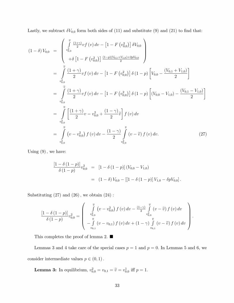
Lastly, we subtract V0,0 form both sides of (11) and substitute (9) and (21) to find that:
(1 )V0,0 =
0
BBB@
vR
v20,0
(1+)2vf (v) dv
1 F
v20,0V0,0
+1 F
v20,0 (1p)(V0,1+V1,0)+2pV0,0
2
1
CCCA
=
vZ
v20,0
(1 + )
2vf (v) dv
1 F
v20,0 (1 p)
V0,0
(V0,1 + V1,0)
2
=
vZ
v20,0
(1 + )
2vf (v) dv
1 F
v20,0 (1 p)
(V0,0 V1,0)
(V0,1 V1,0)2
=
vZ
v20,0
(1 + )
2v v20,0 +
(1 )2
evf (v) dv
=
vZ
v20,0
v v20,0
f (v) dv
(1 )2
vZ
v20,0
(v ev) f (v) dv. (27)
Using (9) , we have:
[1 (1 p)] (1 p)
v20,0 = [1 (1 p)] (V0,0 V1,0)
= (1 )V0,0 [[1 (1 p)]V1,0 pV0,0] .
Substituting (27) and (26) , we obtain (24) :
[1 (1 p)] (1 p)
v20,0 =
0
BBBB@
vR
v20,0
v v20,0
f (v) dv (1)
2
vR
v20,0
(v ev) f (v) dv
vRv0,1
(v v0,1) f (v) dv + (1 )vRv0,1
(v ev) f (v) dv
1
CCCCA.
This completes the proof of lemma 2.
Lemmas 3 and 4 take care of the special cases p = 1 and p = 0. In Lemmas 5 and 6, we
consider intermediate values p 2 (0, 1) .
Lemma 3: In equilibrium, v20,0 = v0,1 = ev = v10,0 i§ p = 1.
33

Proof of Lemma 3: If p = 1, then the system (5)-(11) immediately implies that
v20,0 = v0,1 = v10,0 = 0, and by its definition, also, ev = 0.
Suppose, v20,0 = v0,1 = ev = v10,0 and p < 1. Then substituting v0,1 for v20,0 and ev into (24) ,
we have
[1 (1 p)] (1 p)
v0,1 =(1 )2
vZ
v0,1
(v v0,1) f (v) dv
<
vZ
v0,1
(v v0,1) f (v) dv =[1 (1 p)] (1 p)
v0,1 from (22) ,
which is a contradiction. This completes the proof of Lemma 3.
In the next lemma, we consider the case p = 0.
Lemma 4: When p = 0, we have ev = v0,1 > v20,0.
Proof of Lemma 4: Let us define the function g (.) as in equation (17) . When p = 0,
from (23) and (22) , we have
g (ev) = g (v0,1) = 0) ev = v0,1.
Substituting it into (24) , we have
gv20,0=
[1 (1 p)] (1 p)
v20,0 vZ
v20,0
v v20,0
f (v) dv
= (1 )2
vZ
v20,0
(v ev) f (v) dv vZ
v0,1
(v v0,1) f (v) dv + (1 )vZ
v0,1
(v ev) f (v) dv
=
(1 )2
vZ
v20,0
(v ev) f (v) dv vZ
ev
(v ev) f (v) dv.
Because g is a strictly increasing function, if gv20,0= 0, then g
v20,0= 0 = g (ev) implies
that ev = v0,1 = v20,0 which, as we showed earlier, holds i§ p = 1. A contradiction! If
34
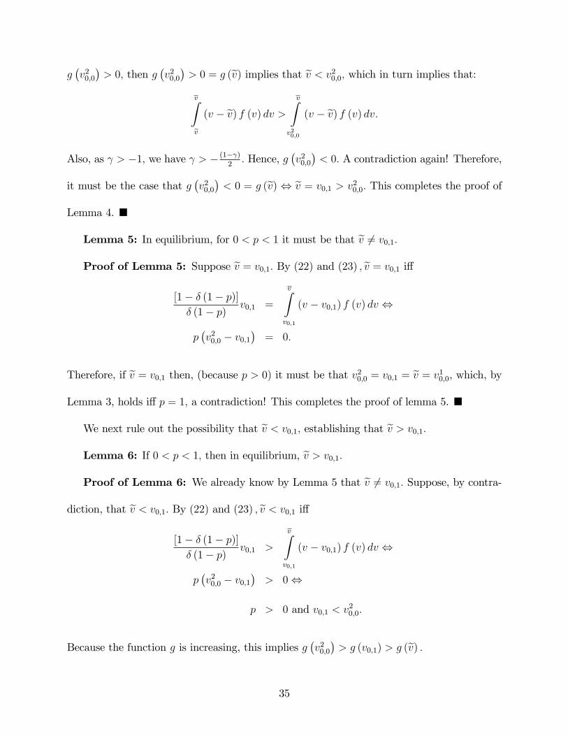
gv20,0> 0, then g
v20,0> 0 = g (ev) implies that ev < v20,0, which in turn implies that:
vZ
ev
(v ev) f (v) dv >vZ
v20,0
(v ev) f (v) dv.
Also, as > 1, we have > (1)2. Hence, g
v20,0< 0. A contradiction again! Therefore,
it must be the case that gv20,0< 0 = g (ev) , ev = v0,1 > v20,0. This completes the proof of
Lemma 4.
Lemma 5: In equilibrium, for 0 < p < 1 it must be that ev 6= v0,1.
Proof of Lemma 5: Suppose ev = v0,1. By (22) and (23) , ev = v0,1 i§
[1 (1 p)] (1 p)
v0,1 =
vZ
v0,1
(v v0,1) f (v) dv ,
pv20,0 v0,1
= 0.
Therefore, if ev = v0,1 then, (because p > 0) it must be that v20,0 = v0,1 = ev = v10,0, which, by
Lemma 3, holds i§ p = 1, a contradiction! This completes the proof of lemma 5.
We next rule out the possibility that ev < v0,1, establishing that ev > v0,1.
Lemma 6: If 0 < p < 1, then in equilibrium, ev > v0,1.
Proof of Lemma 6: We already know by Lemma 5 that ev 6= v0,1. Suppose, by contra-
diction, that ev < v0,1. By (22) and (23) , ev < v0,1 i§
[1 (1 p)] (1 p)
v0,1 >
vZ
v0,1
(v v0,1) f (v) dv ,
pv20,0 v0,1
> 0,
p > 0 and v0,1 < v20,0.
Because the function g is increasing, this implies gv20,0> g (v0,1) > g (ev) .
35

However, by the definition of g, and from (23) and (24) , we have
gv20,0 g (v0,1)
=
0
BBBBB@
2
4 [1(1p)](1p) v
20,0
vR
v20,0
v v20,0
f (v) dv
3
5
"[1(1p)](1p) v0,1
vRv0,1
(v v0,1) f (v) dv
#
1
CCCCCA
=
2
4 (1)2
vR
v20,0
(v ev) f (v) dv vRv0,1
(v v0,1) f (v) dv + (1 )vRv0,1
(v ev) f (v) dv
3
5
"[1(1p)](1p) v0,1
vRv0,1
(v v0,1) f (v) dv
#
=
0
BBBB@
(1)2
vR
v20,0
(v ev) f (v) dv vRv0,1
(v ev) f (v) dv
+vRv0,1
(v ev) f (v) dv [1(1p)](1p) v0,1
1
CCCCA
=
0
BBB@
(1)2
vR
v20,0
(v ev) f (v) dv vRv0,1
(v ev) f (v) dv
+ [1(1p)](1p) ev
[1(1p)](1p) v0,1
1
CCCA, from (22)
= (1 )2
vZ
v20,0
(v ev) f (v) dv vZ
v0,1
(v ev) f (v) dv [1 (1 p)] (1 p)
(v0,1 ev) .
The last term is positive (with a negative sign in the front) because ev < v0,1.We argued that
v0,1 > ev implies that v20,0 > v0,1 > ev, which in turn implies that:
vZ
v0,1
(v ev) f (v) dv >vZ
v20,0
(v ev) f (v) dv.
Also, > (1)2
always because 2 (1, 1) . Hence,2
64(1 )2
vZ
v20,0
(v ev) f (v) dv vZ
v0,1
(v ev) f (v) dv
3
75 < 0,
36

which means thatgv20,0 g (v0,1)
< 0. A contradiction! Therefore, it cannot be the case
that v20,0 > v0,1 and thus v0,1 > ev is not possible. Therefore, for all p > 0, it has to be the
case that ev > v0,1. This completes the proof of Lemma 6.
To complete the proof of Proposition 3, note that ev > v0,1 holds true i§ p > 0 and
v0,1 > v20,0. To argue this, recall that ev is the solution to g (ev) (defined in (18)) which is an
increasing function. Therefore, ev > v0,1 if and only if g (v0,1) < 0 which holds true if and
only if:
[1 (1 p)] (1 p)
v0,1 <
vZ
v0,1
(v v0,1) f (v) dv ,
pv20,0 v0,1
< 0,
p > 0 and v0,1 > v20,0.
We know from Lemma 6 that for all 0 < p < 1, ev > v0,1, and we have just shown that
v0,1 > v20,0, together these facts imply that v
10,0 = ev > v20,0.
Combining with our finding in Lemma 4 for the case p = 0, we conclude that, for all
0 p < 1, we have v10,0 = ev v0,1 > v20,0.
Proof of Proposition 4. From the proof of Lemma 1, we know that v0 is the solution
to g(v0) = 0, where g (.) is an increasing function defined in (17).
From the proof of Proposition 3, we know that v10,0 = ev > v0,1 for all p 2 (0, 1) and hence
we can rewrite (22) as follows:
[1 (1 p)] (1 p)
v10,0 =
vZ
v0,1
v v10,0
f (v) dv
or, gv10,0=
v10,0Z
v0,1
v10,0 v
f (v) dv < 0 = g (v0) .
37

This implies that v10,0 < v0.
Proof of Proposition 5. Note that when p = 1, we have w1 = w0 = 0.
Consider p < 1. Using (13) , we can re-write (14) as follows:
W1 = (1 + )
vZ
w1
(v w1) f (v) dv + (pW0 + (1 p)W1) . (28)
Similarly, using (15) , we can re-write (16) as follows:
W0 = (1 + )
vZ
w0
(v w0) f (v) dv + W0. (29)
Substituting the two equations above into (15) and re-arranging, we get:
(1 + )w0 = (1 p)
2
6664
(1 + )vRw0
(v w0) f (v) dv
(1 + )vRw1
(v w1) f (v) dv + (1 + )w0
3
7775
or,[1 (1 p)] (1 p)
w0 =
vZ
w0
(v w0) f (v) dv vZ
w1
(v w1) f (v) dv. (30)
Again, substituting (12) , (15) and (28) into (13) , we get:
(1 + )w1 = (pW0 + (1 p)W1)
1 (1 p)2p2W0 + 2p (1 p)W1
= (1 p)2
1 (1 p)2 (1 )W0
"1
2p1 (1 p)2
#(1 + )w0
= (1 p)2
1 (1 p)2 (1 + )
vZ
w0
(v w0) f (v) dv
"1
2p1 (1 p)2
#(1 + )w0.
Substituting (30) and re-arranging, we get:
w1 = (1 p)2
1 (1 p)2vZ
w1
(v w1) f (v) dv +p
1 (1 p)2w0
or,
[1 (1 p)] (1 p)
w1 =
vZ
w1
(v w1) f (v) dv +p
(1 p)2(w0 w1) . (31)
38
As we have done in the previous proofs, we can re-write (30) and (31) as follows:
g (w0) = vZ
w1
(v w1) f (v) dv, (32)
g (w1) =p
(1 p)2(w0 w1) , (33)
where g (.) is an increasing function defined as in (17) .
For all p < 1, if w0 w1, then g (w1) 0 > g (w0) which implies w1 > w0, a contradiction!
Hence, w1 > w0 for all p < 1.
Proof of Proposition 6. Note that we assume project values are drawn from the same
distribution in either the two projects or the single project capacity model. From the proof
of Lemma 1, we know that v0 is the solution to a strictly increasing function g (v0) = 0.
From the proof of Proposition 5, we know that w1 > w0 for all p < 1 and by (33) in the
proof of Proposition 5, we know that 0 > g (w1) . It follows that:
g (v0) = 0 > g (w1) > g (w0) .
This implies that v0 > w1 > w0.
Proof of Proposition 7. We follow three steps to prove this proposition.
Step 1: We argue that the optimal project adoption strategy of the 2-projects capacity
firm yields a value that is at least as large as the sum of equilibrium values of the two firms
in the game, W0 2V0,0. The reason why this is true is that the 2-projects capacity decision
maker can mimic the adoption behavior of the strategic firms by setting thresholds:
w0 = v20,0 and w1 = v0,1.
Under this assumption, a project is implemented by the decision maker if and only if one of
the firms would have adopted the project in the game. Under this adoption strategy, it can
39
be shown that: 8>>>>>><
>>>>>>:
W1 = (V0,1 + V1,0)
W0 = 2V0,0
W2 = 2V1,1
solves the system of equations (12), (14) and (16) that defines values for given thresholds in
the 2-projects capacity problem. Because the 2-projects capacity decision maker can achieve
at least 2V0,0 in state 0, it must be that in the optimal strategy, W0 2V0,0.
Step 2: We have shown in Proposition 3 that v20,0 < v10,0 = ev. This implies that,
vZ
v20,0
v v20,0
f (v) dv >
vZ
v20,0
(v ev) f (v) dv
and hence from (27) , we have:
(1 )2V0,0 = 2
vZ
v20,0
v v20,0
f (v) dv (1 )
vZ
v20,0
(v ev) f (v) dv
> 2
vZ
v20,0
v v20,0
f (v) dv (1 )
vZ
v20,0
v v20,0
f (v) dv
= (1 + )
vZ
v20,0
v v20,0
f (v) dv.
Suppose, by contradiction, that w0 v20,0. Then,
(1)2V0,0 > (1 + )vZ
v20,0
v v20,0
f (v) dv (1 + )
vZ
w0
(v w0) f (v) dv = (1 )W0, by (29) .
But we argued that W0 2V0,0, a contradiction! Hence, it must be that w0 < v20,0.
Step 3: We argue that because v20,0 > w0, it must follow that v0,1 > w1. By contradiction,
if it was the case that v0,1 w1, then, using the definition of g (.) in (17) in the proof of
40
Lemma 1, we have:
g (v0,1) g (w1) because g (.) is increasing
)pv20,0 v0,1
(1 p)2p (w0 w1) (1 p)2
by (23) and (33)
)v20,0 v0,1
(w0 w1)
)v20,0 w0
(v0,1 w1) 0
) v20,0 w0, a contradiction!
Hence, it must be that v0,1 > w1.
References
[1] Bloch F. and N. Houy. “Optimal Assignment of Durable Objects to Successive Agents.”
Economic Theory, vol. 51(1) (2012), pp. 13-33.
[2] Burdett, Kenneth, and Dale Mortensen. “Wage Di§erentials, Employer Size, and Un-
employment,” International Economic Review, 39(2) (1998), pp. 257—273.
[3] Daughety A. F. and J. F. Reinganum. “On the Economics of Trials: Adversarial Process,
Evidence, and Equilibrium Bias.” Journal of Law, Economics, & Organization, Vol. 16,
No. 2 (2000) pp. 365-394.
[4] Hall, B. H. and Lerner, J. “The Financing of R&D and Innovation.” Hall, B. H. and N.
Rosenberg (eds.), Handbook of the Economics of Innovation, Elsevier-North Holland,
2010.
41
[5] Harris, M. and Raviv,A. “The Capital Budgeting Process: Incentives and Information.”
The Journal of Finance, Vol. 51, No. 4 (1996), pp. 1139-1174.
[6] Hoppe H. “A Strategic Search Model of Technology Adoption and Policy.” Advances
in Applied Microeconomics, Volume 9: Industrial Organization, Michael R. Baye, ed.,
Greenwich, Conn.: JAI Press. (2000) pp. 197-214.
[7] Lee T. and Wilde L. “Market Structure and Innovation: A Reformulation.” The Quar-
terly Journal of Economics, Vol. 94, No. 2 (1980), pp. 429-436.
[8] Lippman S. and J. Mamer. “Preemptive Innovation.” Journal of Economic Theory, vol.
61 (1993), pp. 104-119.
[9] Loury G. C. “Market Structure and Innovation.” The Quarterly Journal of Economics,
Vol. 93, No. 3. (Aug., 1979), pp. 395-410.
[10] McCall, J. J. “Economics of Information and Job Search.” Quarterly Journal of Eco-
nomics, 84(1) (1970), pp. 113—26.
[11] Mortensen, D. T. “A Theory of Wage and Employment Dynamics,” in Microeconomic
Foundations of Employment and Inflation Theory, E. S. Phelps et al., eds. New York:
W. W. Norton, (1970) pp. 124—66.
[12] Mortensen, D. T. and Pissarides, C. A. “New Developments in Models of Search in the
Labour Market.” Centre for Economic Policy Research, London, 1999.
[13] Nicholas, N. “Scientific Management at Merck: An interview with CFO Judy Lewent.”
Harvard Business review, 72(1) (1994), pp. 89-99.
42
[14] Taylor, Curtis R. “Digging for Golden Carrots: An Analysis of Research Tournaments.”
American Economic Review, Vol. 85, No. 4 (Sept., 1995), pp. 872-890.
[15] Pissarides, C. A. “Short-run Equilibrium Dynamics of Unemployment Vacancies, and
Real Wages.” American Economic Review, vol. 75(4) (1995), pages 676-90.
[16] Pissarides, C. A. “Equilibrium Unemployment Theory.” second edition, Cambridge,
MA: MIT Press (2000).
[17] Postel-Vinay, Fabien, and Jean-Marc Robin. “EquilibriumWage Dispersion withWorker
and Employer Heterogeneity,” Econometrica, 70(6) (2002), pp. 2295—2350.
[18] Reinganum, J. F. “Strategic Search Theory.” International Economic Review, Vol. 23,
No. 1 (1982), pp. 1-17.
[19] Reinganum, J. “Nash Equilibrium Search for the Best Alternative.” Journal of Economic
Theory, Vol. 30, No. 1 (1983a), pp. 139-152.
[20] Reinganum, J. “Uncertain Innovation and the Persistence of Monopoly.” American Eco-
nomic Review, vol. 73(4) (1983b) pp. 741-48.
[21] Zhang G. “Moral Hazard in Corporate Investment and the Disciplinary Role of Volun-
tary Capital Rationing.” Management Science, Vol. 43, No. 6 (1997), pp. 737-750.
43