1

Seasonal concentration of tourism demand: Decomposition analysis and marketing implications.

Tourism Management

DOI: 10.1016/j.tourman.2016.04.004

Antonio Fernández-Moralesa (afdez@uma.es), José David Cisneros-Martínezb* (joscismar@uma.es), and Scott McCabec (scott.mccabe@nottingham.ac.uk).

Tourism Management, vol 56, pgs 172-190.

aUniversidad de Málaga, Facultad de Ciencias Económicas y Empresariales, Departamento de Economía Aplicada (Estadística y Econometría), Calle El Ejido, 6, 29071 Málaga, Spain

bUniversidad de Málaga, Facultad de Turismo, Departamento de Economía Aplicada (Estadística y Econometría), Calle León Tolstoi, 4, 29071 Málaga, Spain

cNottingham University Business School, Jubilee Campus, Wollaton Road, Nottingham NG8 1BB, UK

*Corresponding author.

Abstract

This paper analyzes seasonality in the United Kingdom, specifically the English regions in relation to tourists’ place of origin and main travel motivation. The method used is a decomposition of the Gini index, which provides relative marginal effects that facilitate the identification of market segments open to counter-seasonal marketing efforts. This method has been combined with a graphical multivariate technique (biplot), which groups segments according to their seasonality characteristics. Seasonal patterns associated with particular segments differ significantly when studied on a disaggregated basis. Therefore, an adequate level of disaggregation is essential in the design of counter-seasonal strategies. Although this study focuses on British destinations, this methodology could be used as a control and monitoring measure in the regional analysis of any destination, facilitating regular adjustment of regional tourism marketing campaigns to minimize seasonality effects, specifically by targeting the types of tourists less prone to seasonality.

Keywords: Gini index; seasonality; seasonal patterns; seasonal concentration decomposition; tourism demand; regional analysis; United Kingdom; England

1. Introduction

Seasonality is defined as an imbalance between supply and demand in a given tourist destination over the course of the year (Butler, 1994). Seasonal fluctuations are pervasive in the tourism system due to climactic and socio-structural cycles of both destinations and markets. Thus, the factors that lead to seasonality are a seemingly intractable and perennial management issue, identified recently as “one of the most protracted problems facing managers in the tourism sector” (Coshall, Charlesworth, & Page, 2015, p.1604). Research on seasonality has attempted to model seasonal variations, has looked at how destinations adjust to and manage seasonality, and has investigated the policy and marketing implications of seasonality, as well as the strategies and measures used to overcome seasonality, such as extending the season.

There have, though, been few detailed analyses of trends in European Union market demand, although data does exist on the demand perspective (Eurostat, 2015). Due to rises in global mobility over the last two decades, and an embedding of the culture and practice of travel and tourism as a global human activity, tourism markets are becoming increasingly diverse and complex, particularly in the advanced economies. Moreover, there are few analyses of seasonality from a marketing perspective. There is therefore a need for a better understanding of the patterns of demand across international and national markets, in order to identify those markets that are more resilient to seasonality and the best focus for marketing efforts. Demand could be managed more effectively across peak as well as off-peak seasons if there were a clearer understanding of the concentrations of demand. In particular, different types of tourists may be less prone to seasonality; for instance, information on seasonal concentration in relation to tourists’ motivation would provide important marketing information to destination marketers and could provide additional insights about the effectiveness of specific marketing activities, complementing direct evaluation.

Existing studies have mapped seasonal concentrations. The main aim of this paper is to disaggregate such concentrations. The study uses a novel data visualization technique to add value to the

2

application of the Gini index, which has been widely used for the analysis of tourism demand. It can reveal nuances in demand patterns that tend to be lost when the Gini method is applied to aggregate information (Cisneros-Martínez & Fernández-Morales, 2015; Fernández-Morales & Mayorga-Toledano, 2008; Halpern, 2011). The case context for this analysis is the United Kingdom, and in particular, England and its regions, however, this regional analysis could be applied in any other international destination as long as sufficiently disaggregated data are available. In the present study, international tourism and domestic (to the nine English regions) demand on the part of UK tourists (English, Welsh, and Scottish) are disaggregated by tourists’ place of origin and their main motivation for travel.

Tourism is one of the most important industries in the UK. A record number of overseas tourists (32.8 million) visited the UK in 2013, spending £21.0 billion, also a record figure (Visit Britain, 2014a). Based on its direct, indirect and induced GDP impact, travel and tourism generated 6.9% of the United Kingdom’s GDP in 2013 (World Travel & Tourism Council [WTTC], 2013). In England, as in many European destinations, there is concern, however, about the effects of seasonality in the tourist sector. At the institutional level, tackling seasonality has long been recognized as an issue and it is mentioned in the strategic framework of Visit England (VE) as a high-level objective (Visit England, 2014): VE recognizes seasonality as a problem for the industry and policy is directed towards encouraging efforts to mitigate seasonality as part of the growth strategy for tourism. Specific measures include programs in the low seasons to promote a range of tourism products that are less prone to seasonality issues (Visit England, 2014).

To date, there have been few studies of seasonality and its measurement in the UK. None has focused on England and its regions specifically, and no published studies analyze the seasonal behavior of national and international tourists jointly. Koenig-Lewis and Bischoff (2003) examined the seasonality of domestic tourism in the UK, focusing on Wales and classifying tourists by UK nation of origin and by travel motivation. Koenig-Lewis and Bischoff complemented the Gini index with other techniques, such as the coefficient of variation, seasonal ratio, seasonal plot, coefficient of variability, seasonal factors, amplitude ratio, peak season’s share, amplitude ratio and similarity index. Coshall et al. (2015) conducted a regional analysis of the seasonality of international tourism demand in the Scottish regions using the Gini index and the amplitude ratio, where international tourists were classified by travel motivation, using quarterly data. However, in the present study it has been possible to work with monthly data (by the data availability), leading to a more fine-grained analysis. Furthermore, in this study we go a step further in including both national and international tourism demand. Recently, Connell, Page, and Meyer (2015) analyzed both the ability of events put on in the low season to reduce seasonality in Scotland and how individual businesses respond to seasonality effects in time and space; they were able to show the relationship between attractions and events with seasonality at a regional scale. That analysis was conducted with multivariate tests using correspondence analysis, multivariate cluster and MANOVA. The present analysis complements this analysis with the widely used Gini index together with a novel data visualization technique.

2. Seasonality in the Tourism Industry

In the field of tourism, seasonality is defined as the tendency of tourist flows to be concentrated in relatively short periods of the year (Allcock, 1994). Some authors suggest that seasonality is an intrinsic feature of the tourism sector (e.g. Baum & Lundtorp, 2001). It is a widely known feature (Higham & Hinch, 2002), one of the most vexing policy issues in tourism management, and one which has garnered a deal of cross-disciplinary attention in the literature (Baum & Lundtorp, 2001). Generally, the seasonality effects are described in the literature as negative effects, including: labor instability and unemployment (Ashworth and Thomas, 1999; Ball, 1988); income instability, causing difficulties for returns on investment (Butler, 2001; Jang, 2004; Manning & Powers, 1984); and inefficient use of resources and facilities (Sutcliffe & Sinclair, 1980). On the other hand, seasonality does have some potential benefits, in that in can allow managers to take advantage of lulls in demand to undertake maintenance and repair of the facilities (Grant, Human, & Le Pelley, 1997), to tap into available labor markets at specific times (Mourdoukoutas, 1988) and to promote ecological and socio-cultural recovery during the low season (Butler, 1994; Higham & Hinch 2002). Nonetheless, there are few tourism destinations that are not affected adversely in some way or another by the effects of seasonality; indeed, these effects are felt on all aspects of the supply side of tourism, such as the labor market, finance and investment in tourism businesses, all aspects of operations management and planning, as well as marketing. Therefore, most destinations would benefit from a more even distribution of demand that optimizes the utilization of resources and causes the minimum negative impacts associated with seasonal fluctuations of demand.

3

In the first study undertaken on seasonality in tourism (BarOn, 1975), a distinction between natural factors (principally weather) and institutional factors (including culture) was made. Subsequent research has in general terms confirmed these causes and examined different aspects in more detail (Allcock, 1994; Baum & Hagen, 1999; Butler, 1994; Butler & Mao, 1997; Calantone & Johar, 1984; Commons & Page, 2001; Connell et al., 2015; Higham & Hinch, 2002). Koenig-Lewis and Bischoff (2005) present a comprehensive review of the research on seasonality and its causes. Further exemplary reviews have outlined the main causes and consequences, debates and issues in seasonality research (Baum & Lundtorp, 2001; Boffa & Succurro, 2012; Butler & Mao, 1997; Cannas, 2012; Espinet, Fluvia, & Rigall-I-Torrent, 2012; Getz & Nilsson, 2004; Jang, 2004; Kulendran & Wong, 2005). Coshall et al. (2015) categorized studies on seasonality according to whether they investigated the types and causes of seasonality, their impacts and policy implications, or the range of public and private sector interventions that have been made in attempting to mitigate seasonality. Whilst the existing literature most often focuses on the causes of seasonality, such as climactic factors, availability of tourism products, accessibility and marketing mix, Coshall et al. (2015) sought to shift the focus onto the spatial effects of seasonality. Using Scotland as a case context, they challenged the simple distinctions between notions of core and periphery.

Studies of seasonality have been rich and varied in terms of disciplinary perspectives. They have analyzed demand patterns in geographical or economic terms (Lim & McAleer, 2001; Lundtorp, Rassing, & Wanhill, 1999; Koenig-Lewis & Bischoff, 2003, 2004; Rosselló Nadal, Riera Font, & Sansó Rosselló, 2004), looked at spatial variations in demand, and used forecasting and econometric methods to measure the impact of seasonality (e.g. Sutcliffe & Sinclair, 1980). Cisneros-Martinez and Fernandez-Morales (2015) argue that the approach most commonly used to measure seasonality in tourism is based on the estimation of seasonal factors in a time series, either by deviations from moving averages or with other time series methods. This approach has been used in several studies where seasonality in tourism has been analyzed in a given destination (Cuccia & Rizzo, 2011; Donatos & Zairis, 1991; Nieto González, Amate Fortes, & Nieto González, 2000; Pegg, Patterson, & Vila Gariddo, 2012; Sutcliffe & Sinclair, 1980; Yacoumis, 1980). Furthermore, as Duro (2016), Fernandez-Morales (2003), Lundtorp (2001), Rosselló Nadal et al. (2004) and Wanhill (1980) note in their studies, a complementary approach is to estimate indexes which provide a measure of the annual concentration level, such as the Gini index, the Theil index and the coefficients of variation.

However, tourism is a set of interrelated industries and markets that cannot be treated as an isolated sector (Sinclair, 1998). Although measures that address seasonality may derive from either a public policy or a marketing perspective, such as price adjustments either to stimulate demand in low season or to reduce demand in the peak season, there is less evidence on the effects of these programs and fewer studies that have explicitly sought to assess demand from the marketing perspective. In this regard, the additive decomposition of the Gini index used in this study, and previously in the field of tourism (Cisneros-Martínez & Fernández-Morales, 2015, 2016; Duro, 2016; Fernández-Morales & Mayorga-Toledano, 2008; Halpern, 2011), allows the researcher to classify different market segments in relation to their contribution to annual seasonal concentration and their openness to marketing efforts aimed at reducing seasonality. Such information is of the utmost importance, since it can help marketers direct marketing efforts towards those tourists less likely to want to visit a destination only during the peak time of year.

In this paper, we apply in-depth the additive decomposition by demand segments of the Gini index. This seasonal concentration index can also be decomposed by seasons (Duro, 2016; Fernandez-Morales, 2003). However, in this study, only the decomposition of the annual Gini index by segments of demand is performed. Unlike other studies that have used this technique (Duro, 2016; Fernández-Morales & Mayorga-Toledano, 2008), in this paper it has been applied to two demand characteristics: by market origin (with several disaggregations) and by motivation. Another novelty of this work is the application of the decomposition to the matrix of inter-regional tourism flows in a country for the first time. On the other hand, a data visualization technique (the biplot) is introduced as a tool of analysis for the results of the decomposition components. This multivariate graphical technique facilitates the interpretation of the estimated components and the classification of the segments.

3. Data Sources and Methodology 3.1. Data sources

At the country level, for the analysis of seasonal concentration in the UK, both domestic and international tourism demand figures have been utilized. For domestic tourists, monthly data (number of trips made by UK residents) from the United Kingdom Tourism Survey (UKTS) from 2007 to 2013

4

were obtained. In January 2011, the survey was renamed the Great Britain Tourism Survey (GBTS)1, which counts only the number of trips made by residents of Great Britain (i.e. excluding trips made by residents of Northern Ireland, since these were then recorded by the Northern Ireland Statistics and Research Agency [NISRA]). In this study, it has not been possible to count the trips made by residents in Northern Ireland for 2011, 2012 and 2013 because the NISRA uses quarterly data to represent the results of their tourism surveys (NISRA, 2014), unlike the GBTS which uses monthly data (Visit Britain, 2014b) and therefore, because they are based on different frequencies, these surveys are not directly comparable. For this reason, the results should be interpreted with caution since from 2011 to 2013 they are based only on residents of Great Britain.

In addition, monthly data from the International Passenger Survey (IPS)2 from 2007 to 2013 have been used for the identification of international tourists. The results of IPS are primarily used, among others, to provide information about international tourism. This survey collects information about the number of trips made by international tourists visiting the UK. For a more detailed analysis of international tourists, we have selected one of the classifications established by the IPS, grouping tourists by origin as follow:

EU15 (all countries that joined the European Union before January 1st 2004): Austria, Belgium, Denmark, Finland, France, Germany, Greece, Irish Republic, Italy, Luxembourg, Netherlands, Portugal, Spain and Sweden.

Other EU (all countries that joined the European Union from 1st January 2004 onwards): Bulgaria, Croatia, Cyprus, Czech Republic, Estonia, Hungary, Latvia, Lithuania, Malta, Poland, Romania, Slovakia and Slovenia.

Rest Europe (European countries not included in EU15 and Other EU): Gibraltar, Iceland, Norway, Russia, Switzerland and Turkey and others.

North America: Canada and USA. Other countries: Australia, Caribbean Island, China (Hong Kong), Egypt, India, Israel, Japan,

Mexico, New Zealand, Other Africa, Other Asia, Other Central & South America, Pakistan, South Africa, Sri Lanka, Thailand, Tunisia, United Arab Emirates, other China, other North America, other Middle East and others.

Finally, in order to disaggregate international tourists further, to enable us to identify which markets are ‘favorable’, we have taken the quarterly data from Travelpac3 for 2013, which consist of a series of files derived from the IPS recording specific details of country of origin.

The selection of the surveys mentioned (UKTS / GBTS and IPS / Travelpac) is due to several reasons. First, they are the only surveys available that allow the identification of the domestic and international tourism demand in the UK. Second, all of these surveys use the visits as unit of measure, which are counted as number of trips, being therefore, comparable. Moreover, these surveys use monthly data except Travelpac, which uses quarterly data. For this reason, although the results obtained from this quarterly variable are not directly comparable to those obtained from the IPS monthly data, because they are presented in different frequencies, many conclusions can be drawn about the level of seasonal concentration produced by foreign tourists by countries of origin. Finally, it is also important to note that there has been no methodological change in any of the surveys used during the years analyzed in this study (Visit England, 2013; ONS, 2010; ONS, 2015)

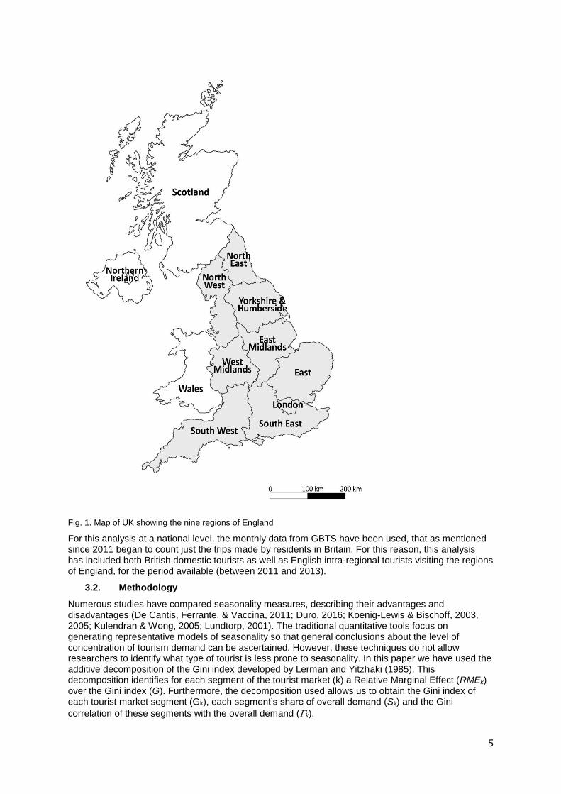
On the other hand, at the national level, ‘seasonal concentration’ of tourists who visited the regions of England is analyzed by national origin for those resident in either Scotland or Wales and by regional origin for those resident in England (East, East Midlands, London, North East, North West, South East, South West, West Midlands, and Yorkshire and Humberside) (Fig. 1).

1 This monthly survey covers overnight trips taken for any purpose, including holidays, business, or visiting friends and relatives. The current survey methodology started in May 2005. The UKTS (GBTS from January 2011) comprises: 100,000 face-to-face interviews per annum, conducted in-home. A weekly sample size of around 2,000 adults aged 16 or over - representative of the UK (GB from 2011) population in relation to various demographic characteristics including gender, age group, socio-economic group, and geographical location (Visit England, 2013). 2 This survey collects information about passengers entering and leaving the UK, and has been running continuously since 1961. Survey data is collected on the IPS via face-to-face interviews with passengers passing through ports and on routes into and out of the UK. The IPS methodology involves conducting between 700,000 and 800,000 interviews a year, of which over 250,000 are used to produce estimates of Overseas Travel and Tourism patterns (Office for National Statistics [ONS], 2015). 3 Travelpac is a simplified version of the IPS database containing 14 of the most widely used categorical and continuous variables. The categorical variables give counts of trips falling into various categories, and include the ones used in this study (the year, the quarter and the country of residence for overseas residents). In addition, there are four continuous variables as the visits, the one selected for this study (ONS, 2010).

5

Fig. 1. Map of UK showing the nine regions of England

For this analysis at a national level, the monthly data from GBTS have been used, that as mentioned since 2011 began to count just the trips made by residents in Britain. For this reason, this analysis has included both British domestic tourists as well as English intra-regional tourists visiting the regions of England, for the period available (between 2011 and 2013).

3.2. Methodology

Numerous studies have compared seasonality measures, describing their advantages and disadvantages (De Cantis, Ferrante, & Vaccina, 2011; Duro, 2016; Koenig-Lewis & Bischoff, 2003, 2005; Kulendran & Wong, 2005; Lundtorp, 2001). The traditional quantitative tools focus on generating representative models of seasonality so that general conclusions about the level of concentration of tourism demand can be ascertained. However, these techniques do not allow researchers to identify what type of tourist is less prone to seasonality. In this paper we have used the additive decomposition of the Gini index developed by Lerman and Yitzhaki (1985). This decomposition identifies for each segment of the tourist market (k) a Relative Marginal Effect (RMEk) over the Gini index (G). Furthermore, the decomposition used allows us to obtain the Gini index of each tourist market segment (Gk), each segment’s share of overall demand (Sk) and the Gini

correlation of these segments with the overall demand (k).

6

There are other available decompositions by sources of concentration indices, like the Theil index and the Coefficient of Variation decompositions that are analysed with recent Spanish tourism data by Duro (2016). We chose the Gini decomposition mainly because it is the most commonly used in the analysis of tourism seasonality and also facilitates the identification of segments with favourable impact for reducing seasonality via the estimation of RME.

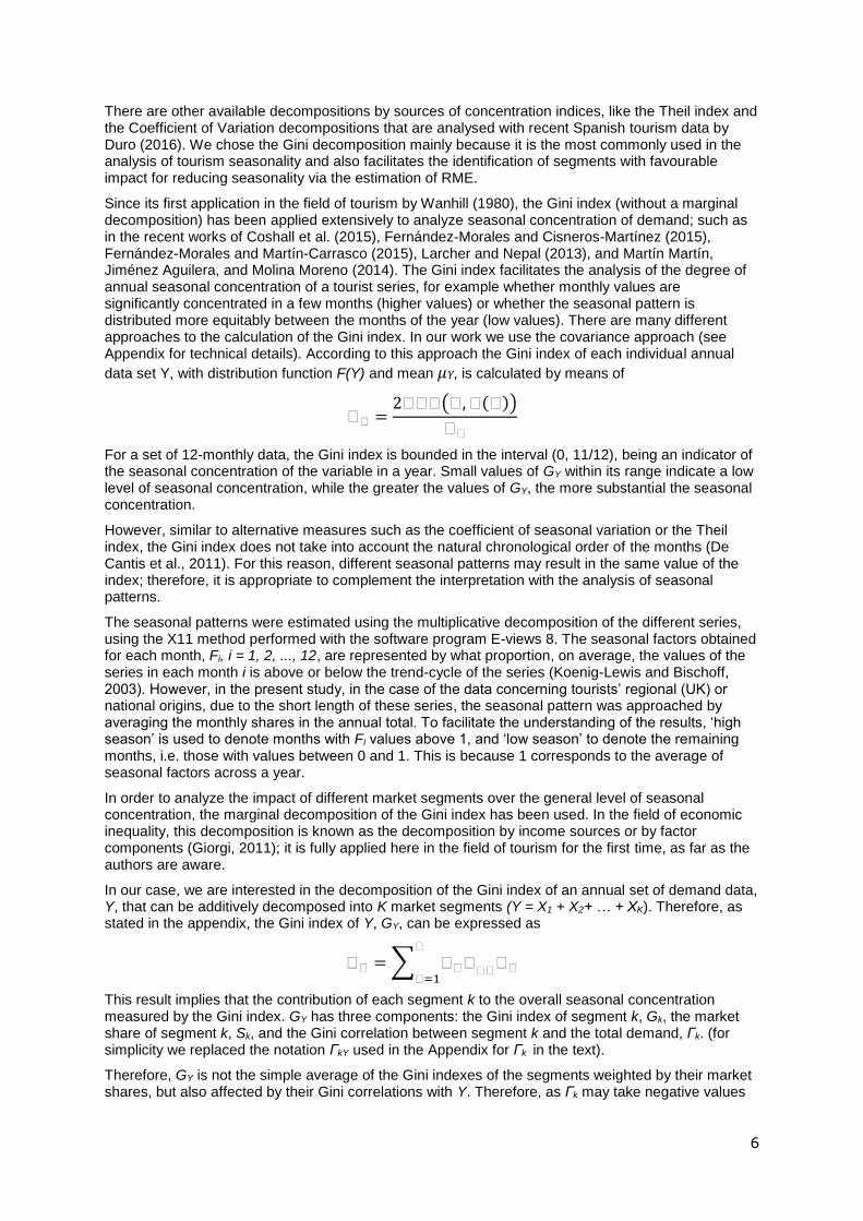
Since its first application in the field of tourism by Wanhill (1980), the Gini index (without a marginal decomposition) has been applied extensively to analyze seasonal concentration of demand; such as in the recent works of Coshall et al. (2015), Fernández-Morales and Cisneros-Martínez (2015), Fernández-Morales and Martín-Carrasco (2015), Larcher and Nepal (2013), and Martín Martín, Jiménez Aguilera, and Molina Moreno (2014). The Gini index facilitates the analysis of the degree of annual seasonal concentration of a tourist series, for example whether monthly values are significantly concentrated in a few months (higher values) or whether the seasonal pattern is distributed more equitably between the months of the year (low values). There are many different approaches to the calculation of the Gini index. In our work we use the covariance approach (see Appendix for technical details). According to this approach the Gini index of each individual annual

data set Y, with distribution function F(Y) and mean µY, is calculated by means of

𝐺𝐺 =2𝐺𝐺𝐺(𝐺, 𝐺(𝐺))

𝐺𝐺

For a set of 12-monthly data, the Gini index is bounded in the interval (0, 11/12), being an indicator of the seasonal concentration of the variable in a year. Small values of GY within its range indicate a low level of seasonal concentration, while the greater the values of GY, the more substantial the seasonal concentration.

However, similar to alternative measures such as the coefficient of seasonal variation or the Theil index, the Gini index does not take into account the natural chronological order of the months (De Cantis et al., 2011). For this reason, different seasonal patterns may result in the same value of the index; therefore, it is appropriate to complement the interpretation with the analysis of seasonal patterns.

The seasonal patterns were estimated using the multiplicative decomposition of the different series, using the X11 method performed with the software program E-views 8. The seasonal factors obtained for each month, Fi, i = 1, 2, ..., 12, are represented by what proportion, on average, the values of the series in each month i is above or below the trend-cycle of the series (Koenig-Lewis and Bischoff, 2003). However, in the present study, in the case of the data concerning tourists’ regional (UK) or national origins, due to the short length of these series, the seasonal pattern was approached by averaging the monthly shares in the annual total. To facilitate the understanding of the results, ‘high season’ is used to denote months with Fi values above 1, and ‘low season’ to denote the remaining months, i.e. those with values between 0 and 1. This is because 1 corresponds to the average of seasonal factors across a year.

In order to analyze the impact of different market segments over the general level of seasonal concentration, the marginal decomposition of the Gini index has been used. In the field of economic inequality, this decomposition is known as the decomposition by income sources or by factor components (Giorgi, 2011); it is fully applied here in the field of tourism for the first time, as far as the authors are aware.

In our case, we are interested in the decomposition of the Gini index of an annual set of demand data, Y, that can be additively decomposed into K market segments (Y = X1 + X2+ … + XK). Therefore, as stated in the appendix, the Gini index of Y, GY, can be expressed as

𝐺𝐺 = ∑ 𝐺𝐺𝐺𝐺𝐺

𝐺𝐺

𝐺

𝐺=1

This result implies that the contribution of each segment k to the overall seasonal concentration measured by the Gini index. GY has three components: the Gini index of segment k, Gk, the market share of segment k, Sk, and the Gini correlation between segment k and the total demand, Γk. (for simplicity we replaced the notation ΓkY used in the Appendix for Γk in the text).

Therefore, GY is not the simple average of the Gini indexes of the segments weighted by their market shares, but also affected by their Gini correlations with Y. Therefore, as Γk may take negative values

7

(when the distribution along the year of segment k is divergent from that of Y) some segments can contribute to a reduction in the overall level of seasonal concentration. So, in order to get a complete analysis of seasonal concentration of segmented markets using the Gini index, it is necessary to complement the analysis with the Gini correlations as well as with the market shares and the Gini indexes of each segment.

In addition, it would also be very useful to obtain the marginal effect of a change in any of the components of the series over the total Gini index. Following Lerman and Yitzhaki (1985), the Relative Marginal Effect, RMEk, of a small proportional increment (uniformly distributed across the

year) of component k, 𝐺k, over the total Gini index, Gy, is obtained as

𝐺𝐺𝐺𝐺 =𝐺𝐺𝐺𝐺𝐺𝐺

𝐺𝐺

− 𝐺𝐺

Thus, the RMEk of segment k is an indicator of its potential impact on the level of seasonal concentration, since it measures the relative increment or decrement of the overall Gini index associated to the prospective growth of that segment. Importantly, segments (here termed ‘favorable tourists’) with negative RMEk will be those open to efforts that counteract seasonality, as they tend to reduce the overall Gini index.

In order to facilitate the analysis, we classified the level of concentration as follows: concentration is high when Gk values are above 0.25, medium when they are between 0.15 and 0.25, and low when they are below 0.15. ‘Favorable tourists’ are those in segments with RMEk exceeding -0.02 (in absolute magnitude), and conversely ‘unfavorable tourists’ are those with RMEk 0.02 or greater. Finally, those who are in the intermediate values will be considered as somewhat favorable.

The level Sk has been classified with the interval [0.10, 0.20] for a medium level of participation. The values below this range will be considered as a low level of share and higher values as a high level.

Similarly, for the classification of the level of k, the interval [0.0, 0.50] has been set for consideration of a medium Gini correlation.

Finally, a multivariate graphical technique, the biplot, has been used to enrich the study of the Gini decomposition. The biplot projects in a two-dimensional space both the observations and the variables in a set, maintaining the approximate distance between the observations (Rencher & Christensen, 2012). The observations are represented by dots, while arrows represent the variables. The angles between arrows approximate the Gini correlation between them and the length of each arrow is an indication of the variance. In our study, biplots are used to show in a graphical

representation the variables Gk, Sk, k, and RMEk for each of the k components for a destination. All the variables were standardized, resulting in arrows of the same length. The biplots helped in the identification of market segments with similar characteristics and also facilitated the interpretation of the relationships between the three additive components of the Gini index and their influence on RMEk.

4. Results 4.1. Seasonal concentration of tourism in the UK

The seasonal concentration produced by tourists visiting the UK is not very high compared with other international destinations but it is nonetheless desirable to minimize its negative effects. The evolution of the number of trips made by domestic and international tourists visiting the UK in the period 2007-2013 is shown in Fig. 2. This evolution is characterized by its consistency, despite the global economic crisis that began in 2008. By analyzing both domestic and international tourists, it is noted that international tourists exerted less seasonal behavior throughout the period analyzed and indeed were ‘favorable tourists’ in all the years observed.

8

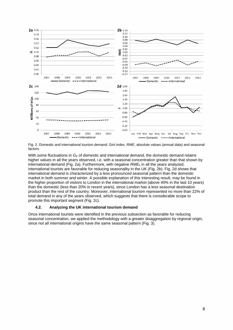
Fig. 2. Domestic and international tourism demand: Gini index, RME, absolute values (annual data) and seasonal factors.

With some fluctuations in GK of domestic and international demand, the domestic demand retains higher values in all the years observed, i.e. with a seasonal concentration greater than that shown by international demand (Fig. 2a). Furthermore, with negative RMEk in all the years analyzed, international tourists are favorable for reducing seasonality in the UK (Fig. 2b). Fig. 2d shows that international demand is characterized by a less pronounced seasonal pattern than the domestic market in both summer and winter. A possible explanation of this interesting result, may be found in the higher proportion of visitors to London in the international market (above 40% in the last 10 years) than the domestic (less than 20% in recent years), since London has a less seasonal destination product than the rest of the country. Moreover, international tourism represented no more than 22% of total demand in any of the years observed, which suggests that there is considerable scope to promote this important segment (Fig. 2c).

4.2. Analyzing the UK international tourism demand

Once international tourists were identified in the previous subsection as favorable for reducing seasonal concentration, we applied the methodology with a greater disaggregation by regional origin, since not all international origins have the same seasonal pattern (Fig. 3).

9

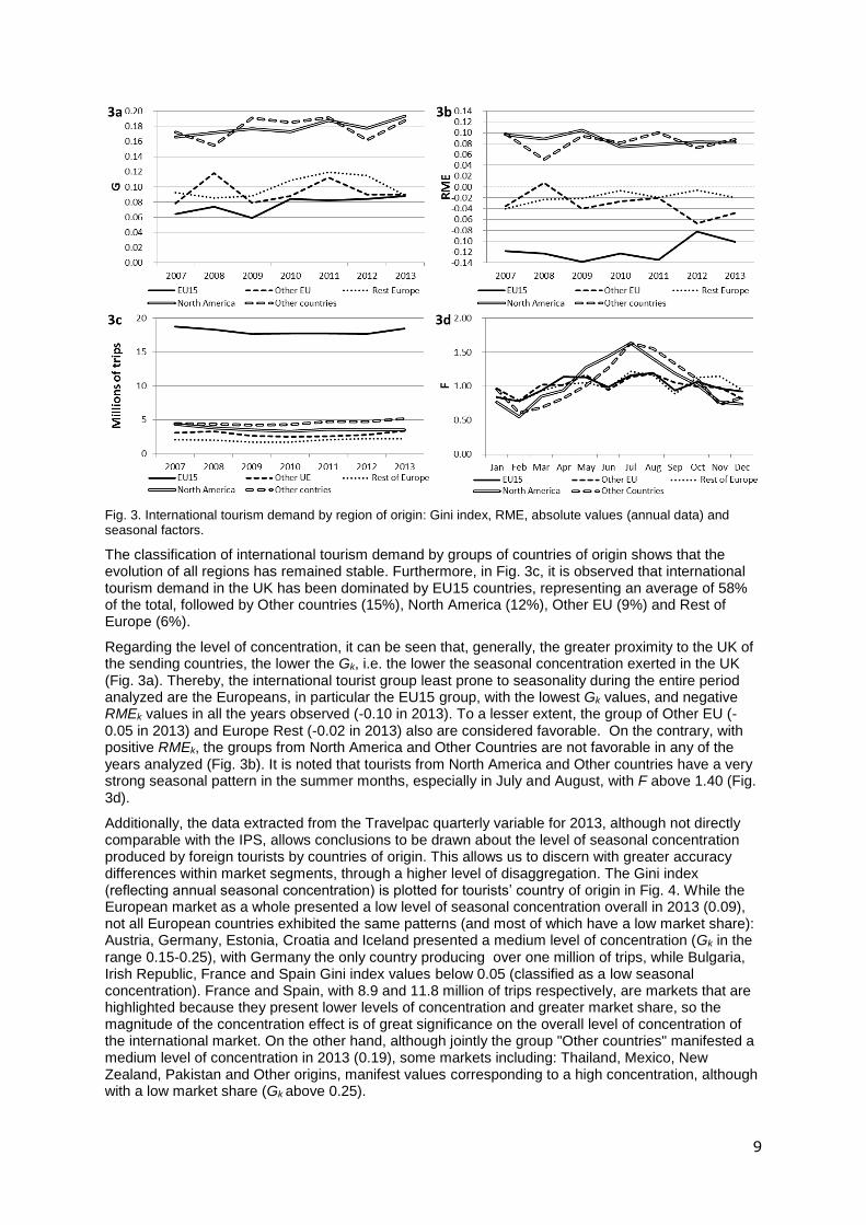
Fig. 3. International tourism demand by region of origin: Gini index, RME, absolute values (annual data) and seasonal factors.

The classification of international tourism demand by groups of countries of origin shows that the evolution of all regions has remained stable. Furthermore, in Fig. 3c, it is observed that international tourism demand in the UK has been dominated by EU15 countries, representing an average of 58% of the total, followed by Other countries (15%), North America (12%), Other EU (9%) and Rest of Europe (6%).

Regarding the level of concentration, it can be seen that, generally, the greater proximity to the UK of the sending countries, the lower the Gk, i.e. the lower the seasonal concentration exerted in the UK (Fig. 3a). Thereby, the international tourist group least prone to seasonality during the entire period analyzed are the Europeans, in particular the EU15 group, with the lowest Gk values, and negative RMEk values in all the years observed (-0.10 in 2013). To a lesser extent, the group of Other EU (-0.05 in 2013) and Europe Rest (-0.02 in 2013) also are considered favorable. On the contrary, with positive RMEk, the groups from North America and Other Countries are not favorable in any of the years analyzed (Fig. 3b). It is noted that tourists from North America and Other countries have a very strong seasonal pattern in the summer months, especially in July and August, with F above 1.40 (Fig. 3d).

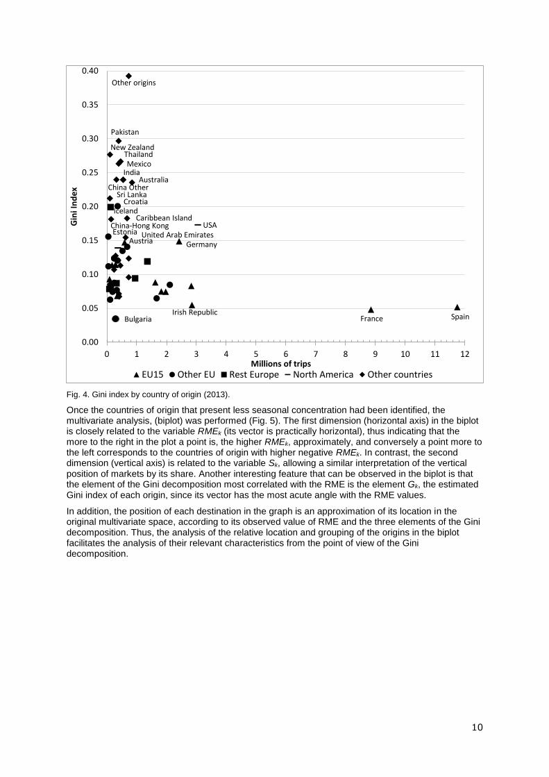
Additionally, the data extracted from the Travelpac quarterly variable for 2013, although not directly comparable with the IPS, allows conclusions to be drawn about the level of seasonal concentration produced by foreign tourists by countries of origin. This allows us to discern with greater accuracy differences within market segments, through a higher level of disaggregation. The Gini index (reflecting annual seasonal concentration) is plotted for tourists’ country of origin in Fig. 4. While the European market as a whole presented a low level of seasonal concentration overall in 2013 (0.09), not all European countries exhibited the same patterns (and most of which have a low market share): Austria, Germany, Estonia, Croatia and Iceland presented a medium level of concentration (Gk in the range 0.15-0.25), with Germany the only country producing over one million of trips, while Bulgaria, Irish Republic, France and Spain Gini index values below 0.05 (classified as a low seasonal concentration). France and Spain, with 8.9 and 11.8 million of trips respectively, are markets that are highlighted because they present lower levels of concentration and greater market share, so the magnitude of the concentration effect is of great significance on the overall level of concentration of the international market. On the other hand, although jointly the group "Other countries" manifested a medium level of concentration in 2013 (0.19), some markets including: Thailand, Mexico, New Zealand, Pakistan and Other origins, manifest values corresponding to a high concentration, although with a low market share (Gk above 0.25).

10

Fig. 4. Gini index by country of origin (2013).

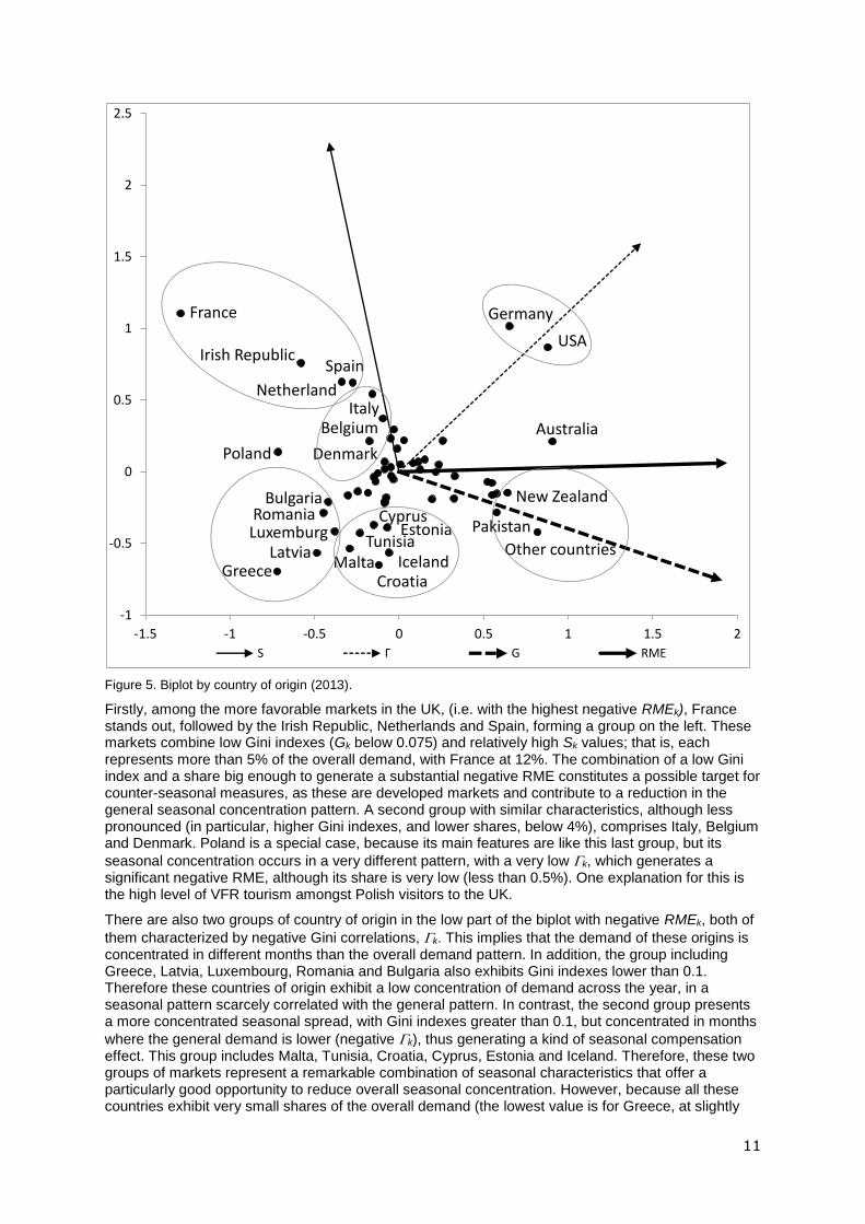
Once the countries of origin that present less seasonal concentration had been identified, the multivariate analysis, (biplot) was performed (Fig. 5). The first dimension (horizontal axis) in the biplot is closely related to the variable RMEk (its vector is practically horizontal), thus indicating that the more to the right in the plot a point is, the higher RMEk, approximately, and conversely a point more to the left corresponds to the countries of origin with higher negative RMEk. In contrast, the second dimension (vertical axis) is related to the variable Sk, allowing a similar interpretation of the vertical position of markets by its share. Another interesting feature that can be observed in the biplot is that the element of the Gini decomposition most correlated with the RME is the element Gk, the estimated Gini index of each origin, since its vector has the most acute angle with the RME values.

In addition, the position of each destination in the graph is an approximation of its location in the original multivariate space, according to its observed value of RME and the three elements of the Gini decomposition. Thus, the analysis of the relative location and grouping of the origins in the biplot facilitates the analysis of their relevant characteristics from the point of view of the Gini decomposition.

Estonia

Sri Lanka

New Zealand

Iceland

China-Hong Kong

Bulgaria

China Other

Croatia

Pakistan

ThailandMexico

Australia

AustriaUnited Arab Emirates

Caribbean Island

Other origins

India

Germany

Irish Republic

USA

France Spain

0.00

0.05

0.10

0.15

0.20

0.25

0.30

0.35

0.40

0 1 2 3 4 5 6 7 8 9 10 11 12

Gin

i In

de

x

Millions of tripsEU15 Other EU Rest Europe North America Other countries

11

Figure 5. Biplot by country of origin (2013).

Firstly, among the more favorable markets in the UK, (i.e. with the highest negative RMEk), France stands out, followed by the Irish Republic, Netherlands and Spain, forming a group on the left. These markets combine low Gini indexes (Gk below 0.075) and relatively high Sk values; that is, each represents more than 5% of the overall demand, with France at 12%. The combination of a low Gini index and a share big enough to generate a substantial negative RME constitutes a possible target for counter-seasonal measures, as these are developed markets and contribute to a reduction in the general seasonal concentration pattern. A second group with similar characteristics, although less pronounced (in particular, higher Gini indexes, and lower shares, below 4%), comprises Italy, Belgium and Denmark. Poland is a special case, because its main features are like this last group, but its

seasonal concentration occurs in a very different pattern, with a very low k, which generates a significant negative RME, although its share is very low (less than 0.5%). One explanation for this is the high level of VFR tourism amongst Polish visitors to the UK.

There are also two groups of country of origin in the low part of the biplot with negative RMEk, both of

them characterized by negative Gini correlations, k. This implies that the demand of these origins is concentrated in different months than the overall demand pattern. In addition, the group including Greece, Latvia, Luxembourg, Romania and Bulgaria also exhibits Gini indexes lower than 0.1. Therefore these countries of origin exhibit a low concentration of demand across the year, in a seasonal pattern scarcely correlated with the general pattern. In contrast, the second group presents a more concentrated seasonal spread, with Gini indexes greater than 0.1, but concentrated in months

where the general demand is lower (negative k), thus generating a kind of seasonal compensation effect. This group includes Malta, Tunisia, Croatia, Cyprus, Estonia and Iceland. Therefore, these two groups of markets represent a remarkable combination of seasonal characteristics that offer a particularly good opportunity to reduce overall seasonal concentration. However, because all these countries exhibit very small shares of the overall demand (the lowest value is for Greece, at slightly

AustraliaBelgium

Bulgaria

Croatia

Cyprus

Denmark

Estonia

France Germany

GreeceIceland

Irish Republic

Italy

LatviaLuxemburg

Malta

Netherland

New Zealand

Poland

Other countries

PakistanRomania

Spain

Tunisia

USA

-1

-0.5

0

0.5

1

1.5

2

2.5

-1.5 -1 -0.5 0 0.5 1 1.5 2

S Γ G RME

12

under -0.5%), their negative RMEk values are reduced compared with other markets. Nonetheless, this could be seen as a chance to focus on these countries in case the reduced shares were an indication of the possibility for market expansion. For these countries, marketing strategies to increase market share would be sufficient to reduce the seasonal effects,

As for the countries of origin with positive RMEk, two distinct groups are highlighted in the biplot:

firstly, Germany and the USA, with the highest k and with high Sk and Gk values; and secondly, New Zealand, Pakistan and the markets grouped under "Other countries", with a reduced Sk value, but also

with the highest Gini indexes, combined with k close to 1. Australia is in an intermediate position between these two groups. The main difference between these markets is the relative share of overall demand, but in general all contribute to a greater seasonal concentration when their demand grows, especially in the case of the more important, such as Germany and the USA. To counter their pro-seasonal effect, strategies that redistribute demand from these countries origins across the year could be designed (Koenig-Lewis & Bischoff 2005). For this, tourism marketers could use (among other instruments) programs to promote low season activities during peak season by designing loyalty programs with benefits, discounts and other incentives that encourage demand to the destination in the low season (Council of Tourism, Commerce and Sport of Andalusia, 2015). Furthermore, it would be important to identify segments within those markets that might increase demand in the low season (Baum & Hagen 1999).

4.3. Analyzing the concentration of the UK tourism demand by motivation

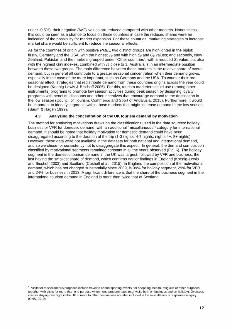
The method for analyzing motivations draws on the classifications used in the data sources: holiday, business or VFR for domestic demand, with an additional ‘miscellaneous’4 category for international demand. It should be noted that holiday motivation for domestic demand could have been disaggregated according to the duration of the trip (1-3 nights; 4-7 nights; nights 4+, 8+ nights). However, these data were not available in the datasets for both national and international demand, and so we chose for consistency not to disaggregate this aspect. In general, the demand composition classified by motivational segments remained constant in all the years observed (Fig. 6). The holiday segment in the domestic tourism demand in the UK was largest, followed by VFR and business, the last having the smallest share of demand, which confirms earlier findings in England (Koenig-Lewis and Bischoff 2003) and Scotland (Coshall et al., 2015). In England the composition of the motivational demand, which has not changed substantially since 2009, is 39% for holiday segment, 29% for VFR and 24% for business in 2013. A significant difference is that the share of the business segment in the international tourism demand in England is more than twice that of Scotland.

4 Visits for miscellaneous purposes include travel to attend sporting events, for shopping, health, religious or other purposes, together with visits for more than one purpose when none predominates (e.g. visits both on business and on holiday). Overseas visitors staying overnight in the UK in route to other destinations are also included in the miscellaneous purposes category. (ONS, 2010).

13

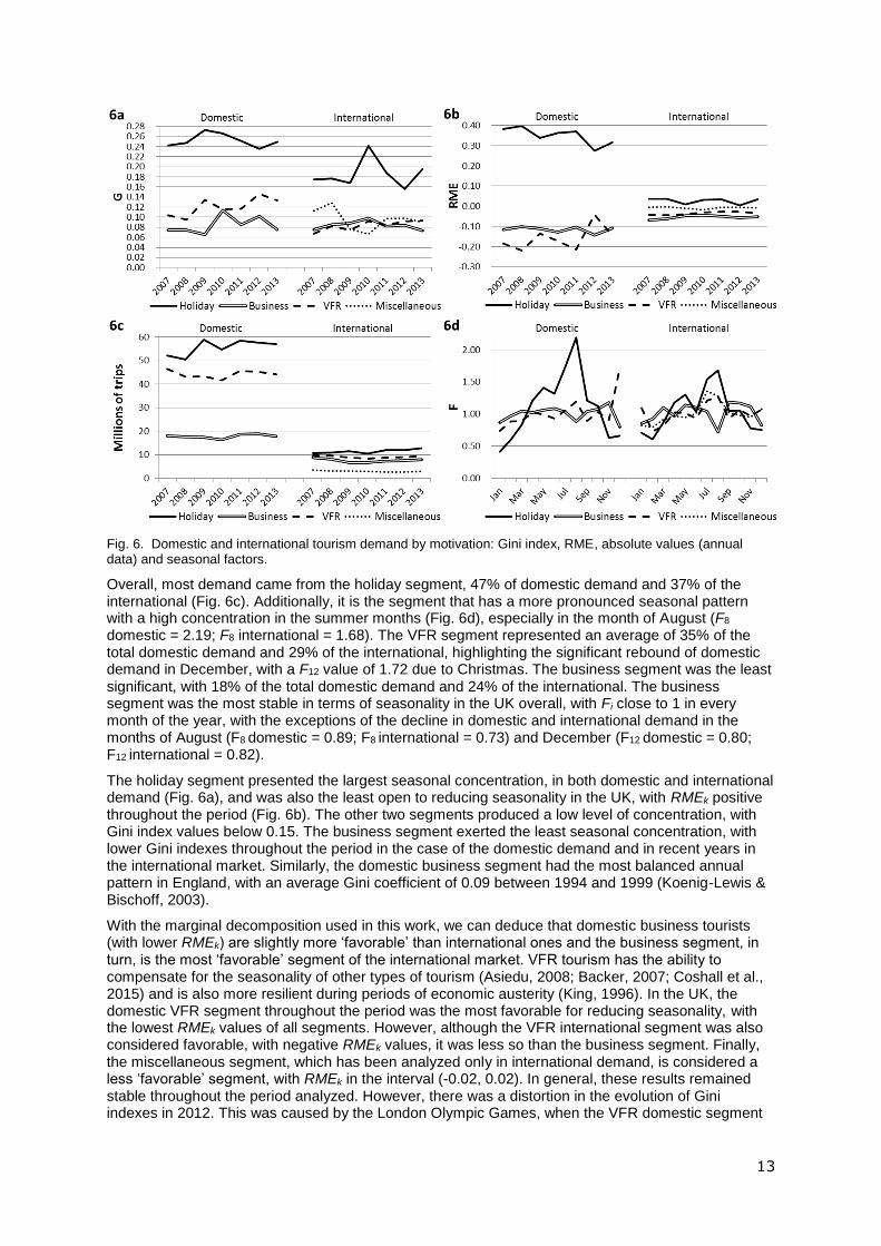
Fig. 6. Domestic and international tourism demand by motivation: Gini index, RME, absolute values (annual data) and seasonal factors.

Overall, most demand came from the holiday segment, 47% of domestic demand and 37% of the international (Fig. 6c). Additionally, it is the segment that has a more pronounced seasonal pattern with a high concentration in the summer months (Fig. 6d), especially in the month of August (F8 domestic = 2.19; F8 international = 1.68). The VFR segment represented an average of 35% of the total domestic demand and 29% of the international, highlighting the significant rebound of domestic demand in December, with a F12 value of 1.72 due to Christmas. The business segment was the least significant, with 18% of the total domestic demand and 24% of the international. The business segment was the most stable in terms of seasonality in the UK overall, with Fi close to 1 in every month of the year, with the exceptions of the decline in domestic and international demand in the months of August (F8 domestic = 0.89; F8 international = 0.73) and December (F12 domestic = 0.80; F12 international = 0.82).

The holiday segment presented the largest seasonal concentration, in both domestic and international demand (Fig. 6a), and was also the least open to reducing seasonality in the UK, with RMEk positive throughout the period (Fig. 6b). The other two segments produced a low level of concentration, with Gini index values below 0.15. The business segment exerted the least seasonal concentration, with lower Gini indexes throughout the period in the case of the domestic demand and in recent years in the international market. Similarly, the domestic business segment had the most balanced annual pattern in England, with an average Gini coefficient of 0.09 between 1994 and 1999 (Koenig-Lewis & Bischoff, 2003).

With the marginal decomposition used in this work, we can deduce that domestic business tourists (with lower RMEk) are slightly more ‘favorable’ than international ones and the business segment, in turn, is the most ‘favorable’ segment of the international market. VFR tourism has the ability to compensate for the seasonality of other types of tourism (Asiedu, 2008; Backer, 2007; Coshall et al., 2015) and is also more resilient during periods of economic austerity (King, 1996). In the UK, the domestic VFR segment throughout the period was the most favorable for reducing seasonality, with the lowest RMEk values of all segments. However, although the VFR international segment was also considered favorable, with negative RMEk values, it was less so than the business segment. Finally, the miscellaneous segment, which has been analyzed only in international demand, is considered a less ‘favorable’ segment, with RMEk in the interval (-0.02, 0.02). In general, these results remained stable throughout the period analyzed. However, there was a distortion in the evolution of Gini indexes in 2012. This was caused by the London Olympic Games, when the VFR domestic segment

14

was considered less favorable, with higher RMEk values, and the holiday segment was less seasonal, with Gk lower than usual during the period.

Going into more detail on the most recent data, and considering that in 2013 the analysis omitted

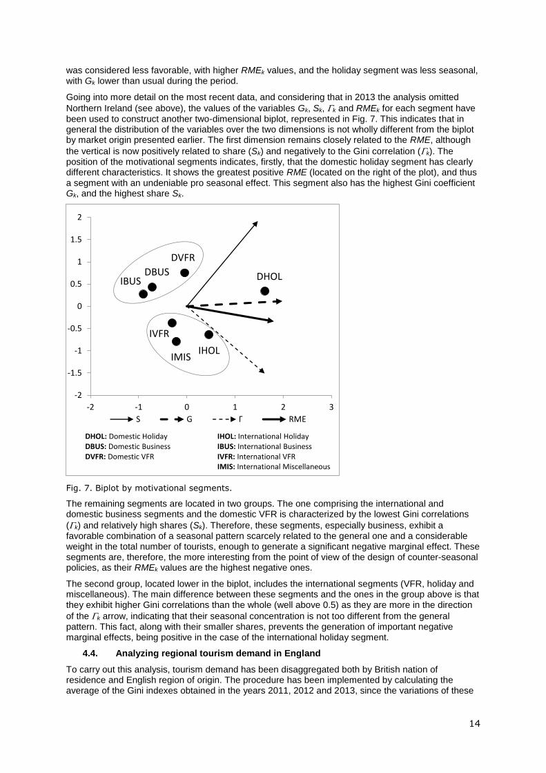
Northern Ireland (see above), the values of the variables Gk, Sk, k and RMEk for each segment have been used to construct another two-dimensional biplot, represented in Fig. 7. This indicates that in general the distribution of the variables over the two dimensions is not wholly different from the biplot by market origin presented earlier. The first dimension remains closely related to the RME, although

the vertical is now positively related to share (Sk) and negatively to the Gini correlation (k). The position of the motivational segments indicates, firstly, that the domestic holiday segment has clearly different characteristics. It shows the greatest positive RME (located on the right of the plot), and thus a segment with an undeniable pro seasonal effect. This segment also has the highest Gini coefficient Gk, and the highest share Sk.

Fig. 7. Biplot by motivational segments.

The remaining segments are located in two groups. The one comprising the international and domestic business segments and the domestic VFR is characterized by the lowest Gini correlations

(k) and relatively high shares (Sk). Therefore, these segments, especially business, exhibit a favorable combination of a seasonal pattern scarcely related to the general one and a considerable weight in the total number of tourists, enough to generate a significant negative marginal effect. These segments are, therefore, the more interesting from the point of view of the design of counter-seasonal policies, as their RMEk values are the highest negative ones.

The second group, located lower in the biplot, includes the international segments (VFR, holiday and miscellaneous). The main difference between these segments and the ones in the group above is that they exhibit higher Gini correlations than the whole (well above 0.5) as they are more in the direction

of the k arrow, indicating that their seasonal concentration is not too different from the general pattern. This fact, along with their smaller shares, prevents the generation of important negative marginal effects, being positive in the case of the international holiday segment.

4.4. Analyzing regional tourism demand in England

To carry out this analysis, tourism demand has been disaggregated both by British nation of residence and English region of origin. The procedure has been implemented by calculating the average of the Gini indexes obtained in the years 2011, 2012 and 2013, since the variations of these

DHOLDBUS

DVFR

IHOL

IBUS

IVFR

IMIS

-2

-1.5

-1

-0.5

0

0.5

1

1.5

2

-2 -1 0 1 2 3

S G Γ RME

DHOL: Domestic Holiday IHOL: International HolidayDBUS: Domestic Business IBUS: International BusinessDVFR: Domestic VFR IVFR: International VFR

IMIS: International Miscellaneous

15

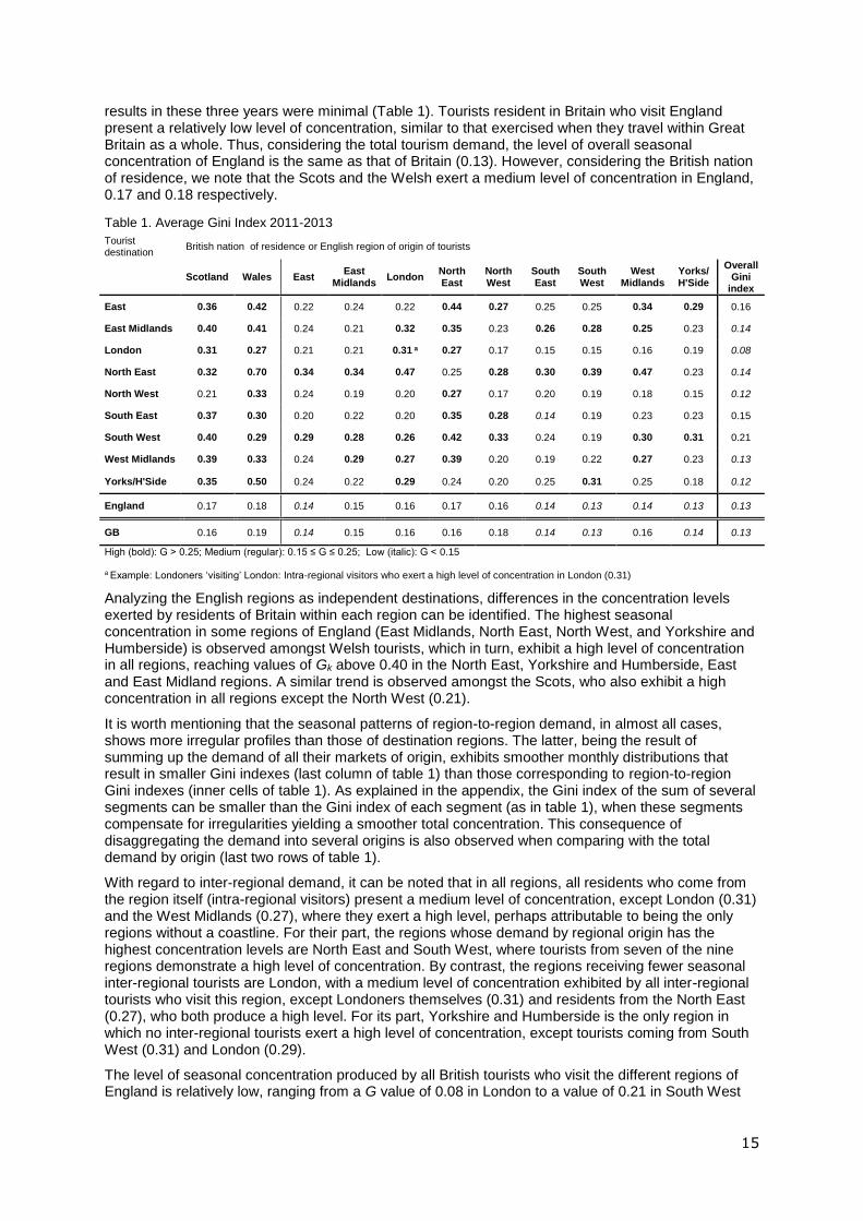
results in these three years were minimal (Table 1). Tourists resident in Britain who visit England present a relatively low level of concentration, similar to that exercised when they travel within Great Britain as a whole. Thus, considering the total tourism demand, the level of overall seasonal concentration of England is the same as that of Britain (0.13). However, considering the British nation of residence, we note that the Scots and the Welsh exert a medium level of concentration in England, 0.17 and 0.18 respectively.

Table 1. Average Gini Index 2011-2013

Tourist destination

British nation of residence or English region of origin of tourists

Scotland Wales East East

Midlands London

North East

North West

South East

South West

West Midlands

Yorks/ H'Side

Overall Gini

index

East 0.36 0.42 0.22 0.24 0.22 0.44 0.27 0.25 0.25 0.34 0.29 0.16

East Midlands 0.40 0.41 0.24 0.21 0.32 0.35 0.23 0.26 0.28 0.25 0.23 0.14

London 0.31 0.27 0.21 0.21 0.31 a 0.27 0.17 0.15 0.15 0.16 0.19 0.08

North East 0.32 0.70 0.34 0.34 0.47 0.25 0.28 0.30 0.39 0.47 0.23 0.14

North West 0.21 0.33 0.24 0.19 0.20 0.27 0.17 0.20 0.19 0.18 0.15 0.12

South East 0.37 0.30 0.20 0.22 0.20 0.35 0.28 0.14 0.19 0.23 0.23 0.15

South West 0.40 0.29 0.29 0.28 0.26 0.42 0.33 0.24 0.19 0.30 0.31 0.21

West Midlands 0.39 0.33 0.24 0.29 0.27 0.39 0.20 0.19 0.22 0.27 0.23 0.13

Yorks/H'Side 0.35 0.50 0.24 0.22 0.29 0.24 0.20 0.25 0.31 0.25 0.18 0.12

England 0.17 0.18 0.14 0.15 0.16 0.17 0.16 0.14 0.13 0.14 0.13 0.13

GB 0.16 0.19 0.14 0.15 0.16 0.16 0.18 0.14 0.13 0.16 0.14 0.13

High (bold): G > 0.25; Medium (regular): 0.15 ≤ G ≤ 0.25; Low (italic): G < 0.15 a Example: Londoners ‘visiting’ London: Intra-regional visitors who exert a high level of concentration in London (0.31)

Analyzing the English regions as independent destinations, differences in the concentration levels exerted by residents of Britain within each region can be identified. The highest seasonal concentration in some regions of England (East Midlands, North East, North West, and Yorkshire and Humberside) is observed amongst Welsh tourists, which in turn, exhibit a high level of concentration in all regions, reaching values of Gk above 0.40 in the North East, Yorkshire and Humberside, East and East Midland regions. A similar trend is observed amongst the Scots, who also exhibit a high concentration in all regions except the North West (0.21).

It is worth mentioning that the seasonal patterns of region-to-region demand, in almost all cases, shows more irregular profiles than those of destination regions. The latter, being the result of summing up the demand of all their markets of origin, exhibits smoother monthly distributions that result in smaller Gini indexes (last column of table 1) than those corresponding to region-to-region Gini indexes (inner cells of table 1). As explained in the appendix, the Gini index of the sum of several segments can be smaller than the Gini index of each segment (as in table 1), when these segments compensate for irregularities yielding a smoother total concentration. This consequence of disaggregating the demand into several origins is also observed when comparing with the total demand by origin (last two rows of table 1).

With regard to inter-regional demand, it can be noted that in all regions, all residents who come from the region itself (intra-regional visitors) present a medium level of concentration, except London (0.31) and the West Midlands (0.27), where they exert a high level, perhaps attributable to being the only regions without a coastline. For their part, the regions whose demand by regional origin has the highest concentration levels are North East and South West, where tourists from seven of the nine regions demonstrate a high level of concentration. By contrast, the regions receiving fewer seasonal inter-regional tourists are London, with a medium level of concentration exhibited by all inter-regional tourists who visit this region, except Londoners themselves (0.31) and residents from the North East (0.27), who both produce a high level. For its part, Yorkshire and Humberside is the only region in which no inter-regional tourists exert a high level of concentration, except tourists coming from South West (0.31) and London (0.29).

The level of seasonal concentration produced by all British tourists who visit the different regions of England is relatively low, ranging from a G value of 0.08 in London to a value of 0.21 in South West

16

(last column of table 1). Finally, it should be pointed out that these results are obtained combining the Gk of the regions of origin of tourists. For example, even though London has the lowest overall level of concentration (G = 0.08), some visitors to the region (e.g. those from Scotland) nevertheless have a medium/high seasonal behavior. Similarly, although most of the inter-regional demands for the North East and South West regions appear to be highly seasonal (with Gk values above 0.25), the overall level of concentration of these regions is medium, with an overall Gini index of 0.14 and 0.21 respectively.

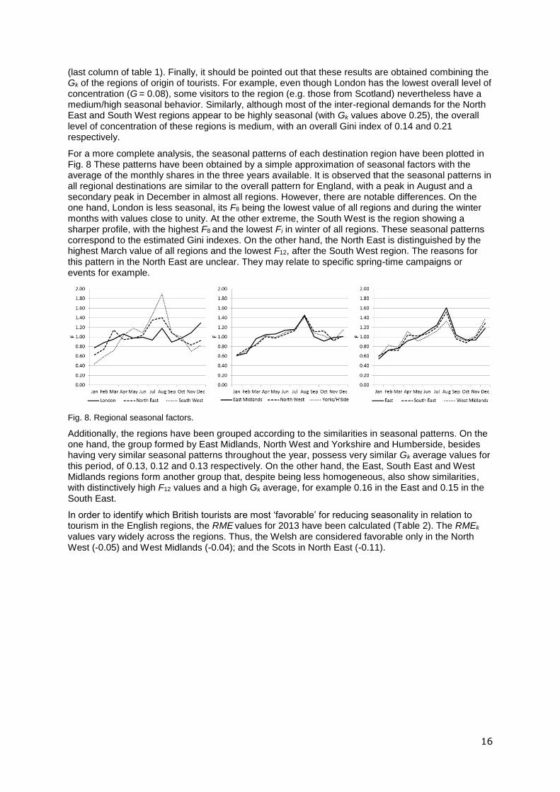
For a more complete analysis, the seasonal patterns of each destination region have been plotted in Fig. 8 These patterns have been obtained by a simple approximation of seasonal factors with the average of the monthly shares in the three years available. It is observed that the seasonal patterns in all regional destinations are similar to the overall pattern for England, with a peak in August and a secondary peak in December in almost all regions. However, there are notable differences. On the one hand, London is less seasonal, its F8 being the lowest value of all regions and during the winter months with values close to unity. At the other extreme, the South West is the region showing a sharper profile, with the highest F8 and the lowest Fi in winter of all regions. These seasonal patterns correspond to the estimated Gini indexes. On the other hand, the North East is distinguished by the highest March value of all regions and the lowest F12, after the South West region. The reasons for this pattern in the North East are unclear. They may relate to specific spring-time campaigns or events for example.

Fig. 8. Regional seasonal factors.

Additionally, the regions have been grouped according to the similarities in seasonal patterns. On the one hand, the group formed by East Midlands, North West and Yorkshire and Humberside, besides having very similar seasonal patterns throughout the year, possess very similar Gk average values for this period, of 0.13, 0.12 and 0.13 respectively. On the other hand, the East, South East and West Midlands regions form another group that, despite being less homogeneous, also show similarities, with distinctively high F12 values and a high Gk average, for example 0.16 in the East and 0.15 in the South East.

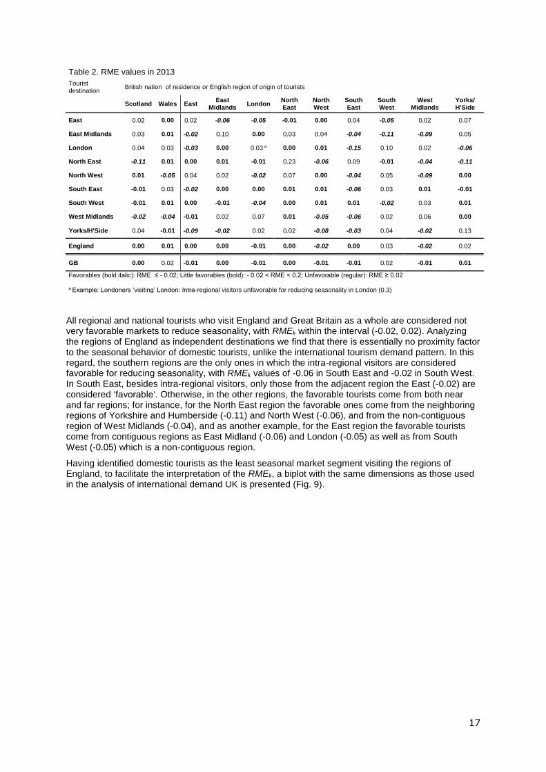
In order to identify which British tourists are most ‘favorable’ for reducing seasonality in relation to tourism in the English regions, the RME values for 2013 have been calculated (Table 2). The RMEk values vary widely across the regions. Thus, the Welsh are considered favorable only in the North West (-0.05) and West Midlands (-0.04); and the Scots in North East (-0.11).

17

Table 2. RME values in 2013

Tourist destination

British nation of residence or English region of origin of tourists

Scotland Wales East East

Midlands London

North East

North West

South East

South West

West Midlands

Yorks/ H'Side

East 0.02 0.00 0.02 -0.06 -0.05 -0.01 0.00 0.04 -0.05 0.02 0.07

East Midlands 0.03 0.01 -0.02 0.10 0.00 0.03 0.04 -0.04 -0.11 -0.09 0.05

London 0.04 0.03 -0.03 0.00 0.03 a 0.00 0.01 -0.15 0.10 0.02 -0.06

North East -0.11 0.01 0.00 0.01 -0.01 0.23 -0.06 0.09 -0.01 -0.04 -0.11

North West 0.01 -0.05 0.04 0.02 -0.02 0.07 0.00 -0.04 0.05 -0.09 0.00

South East -0.01 0.03 -0.02 0.00 0.00 0.01 0.01 -0.06 0.03 0.01 -0.01

South West -0.01 0.01 0.00 -0.01 -0.04 0.00 0.01 0.01 -0.02 0.03 0.01

West Midlands -0.02 -0.04 -0.01 0.02 0.07 0.01 -0.05 -0.06 0.02 0.06 0.00

Yorks/H'Side 0.04 -0.01 -0.09 -0.02 0.02 0.02 -0.08 -0.03 0.04 -0.02 0.13

England 0.00 0.01 0.00 0.00 -0.01 0.00 -0.02 0.00 0.03 -0.02 0.02

GB 0.00 0.02 -0.01 0.00 -0.01 0.00 -0.01 -0.01 0.02 -0.01 0.01

Favorables (bold italic): RME ≤ - 0.02; Little favorables (bold): - 0.02 < RME < 0.2; Unfavorable (regular): RME ≥ 0.02 a Example: Londoners ‘visiting’ London: Intra-regional visitors unfavorable for reducing seasonality in London (0.3)

All regional and national tourists who visit England and Great Britain as a whole are considered not very favorable markets to reduce seasonality, with RMEk within the interval (-0.02, 0.02). Analyzing the regions of England as independent destinations we find that there is essentially no proximity factor to the seasonal behavior of domestic tourists, unlike the international tourism demand pattern. In this regard, the southern regions are the only ones in which the intra-regional visitors are considered favorable for reducing seasonality, with RMEk values of -0.06 in South East and -0.02 in South West. In South East, besides intra-regional visitors, only those from the adjacent region the East (-0.02) are considered ‘favorable‘. Otherwise, in the other regions, the favorable tourists come from both near and far regions; for instance, for the North East region the favorable ones come from the neighboring regions of Yorkshire and Humberside (-0.11) and North West (-0.06), and from the non-contiguous region of West Midlands (-0.04), and as another example, for the East region the favorable tourists come from contiguous regions as East Midland (-0.06) and London (-0.05) as well as from South West (-0.05) which is a non-contiguous region.

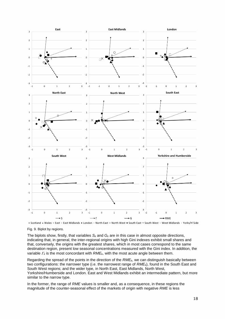
Having identified domestic tourists as the least seasonal market segment visiting the regions of England, to facilitate the interpretation of the RMEk, a biplot with the same dimensions as those used in the analysis of international demand UK is presented (Fig. 9).

18

Fig. 9. Biplot by regions.

The biplots show, firstly, that variables Sk and Gk are in this case in almost opposite directions, indicating that, in general, the inter-regional origins with high Gini indexes exhibit small shares and that, conversely, the origins with the greatest shares, which in most cases correspond to the same destination region, present low seasonal concentrations measured with the Gini index. In addition, the

variable k is the most concordant with RMEk, with the most acute angle between them.

Regarding the spread of the points in the direction of the RMEk, we can distinguish basically between two configurations: the narrower type (i.e. the narrowest range of RMEk), found in the South East and South West regions; and the wider type, in North East, East Midlands, North West, Yorkshire/Humberside and London. East and West Midlands exhibit an intermediate pattern, but more similar to the narrow type.

In the former, the range of RME values is smaller and, as a consequence, in these regions the magnitude of the counter-seasonal effect of the markets of origin with negative RME is less

19

pronounced than in the regions belonging to the second type, which exhibit greater negative RMEk values. So, it is in the regions of the latter type where the identification of markets with the highest RMEk values offers the most interesting opportunities for destination marketers. In general, there are two broad groups or types of origins with substantial negative RMEk values in these regions: (1) those with a small or medium Gini index and medium or high share (above 0.1), and (2) origins that exhibit a high seasonal concentration, but in different months than the general pattern in the region (with medium or small Gini correlation), producing a counter-seasonal effect.

An example of this duality is found in the North East region. Visitors from Yorkshire and Humberside, and North West form a group of the first type characterized by medium Gini indexes, 0.19 and 0.21, and shares of 0.17 and 0.11 (positioned in the positive side of the vertical axis). The low seasonal concentration of these visitors contributes to alleviation of the overall seasonality effects in the region. But, in addition, visitors from Scotland and the West Midlands form another group of origins that can also be target markets for reducing overall seasonality. In this second group, although they show an important seasonal concentration, with Gini indexes of 0.39 and 0.31 (they are located in the negative side of the vertical axis), it occurs in different months from the overall pattern (manifested by negative

Gini correlations, k = -0.04 for both regions of origin), also contributing to a reduction of seasonality in the region.

However, this distinction is not so clear in all the regions. In some cases, like the North West, these two types of origins with negative RMEk, almost overlap, and we find that visitors from the West Midlands show simultaneously a low Gini index (a characteristic of the first type mentioned) and a negative Gini correlation (more distinctive of the second type), a combination that for this region yields the highest negative RMEk, thus being a key target market region for counter-seasonal marketing efforts.

In other regions, the origins with the highest negative RMEk are mainly included in only one type. In the East Midlands, for example, these origins are the South West and West Midlands that belong to the second type with high concentration and negative Gini correlation. In contrast, in London, the outstanding regions of origin are included in the first type, with medium Gini index and shares greater than 0.1.

The intra-regional demand stands out in the direction of Sk in the biplots of all the regions (except London), due to a high share, with Sk values between 0.2 and 0.33, which are also the highest values in each of these regions. This feature accentuates its potential impact, reducing or increasing seasonal concentration. In the regions where the intra-regional demand exhibits a negative RMEk (South East and South West), maintaining or increasing this demand will tend to reduce overall seasonality. However, in four regions the RMEk values for the intra-regional demand were the highest recorded (North East, East Midlands, Yorkshire and Humberside) or the second highest (West Midlands). Although in these four regions the overall Gini index is not very high (in the range 0.12-0.14), the development of a greater intra-regional demand would tend to increase seasonal concentration. It would therefore be advisable in these regions to design strategies aimed at changing the distribution of intra-regional demand across the year. A wide range of measures has been proposed to this end; events and festivals are seemingly the most popular (Koenig-Lewis and Bischoff, 2005). In addition, the provision of counter-seasonal tourism products designed for specific segments such as senior citizens, business travelers, conference travelers and short-break holidaymakers has been suggested (Baum & Hagen, 1999; McEnif, 1992).

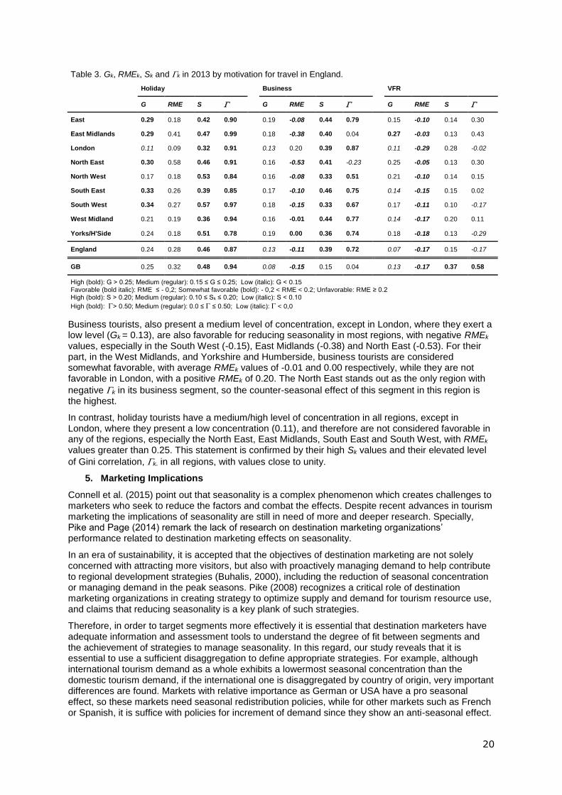
Finally, the seasonal concentration of the English regions according to the main travel motivations of British tourists visiting England has also been evaluated (Table 3). The main results are that VFR segments present a medium level of concentration (Gk) and are considered favorable, with negative RMEk values in all regions, especially in the South East, West Midlands, Yorkshire and Humberside and London, with an average RMEk below -0.15. In addition, these segments’ share of the overall

demand is relatively low, with Sk values below 0.3 and their Gini correlations (k) are also low, even with negative values in the case of Yorkshire and Humberside (-0.29), South West (-0.17) and London (-0.02). This is evidence of possibilities for reducing seasonality by means of increasing these segments’ presence in the overall demand.

20

Table 3. Gk, RMEk, Sk and k in 2013 by motivation for travel in England.

Holiday Business VFR

G RME S G RME S G RME S

East 0.29 0.18 0.42 0.90 0.19 -0.08 0.44 0.79 0.15 -0.10 0.14 0.30

East Midlands 0.29 0.41 0.47 0.99 0.18 -0.38 0.40 0.04 0.27 -0.03 0.13 0.43

London 0.11 0.09 0.32 0.91 0.13 0.20 0.39 0.87 0.11 -0.29 0.28 -0.02

North East 0.30 0.58 0.46 0.91 0.16 -0.53 0.41 -0.23 0.25 -0.05 0.13 0.30

North West 0.17 0.18 0.53 0.84 0.16 -0.08 0.33 0.51 0.21 -0.10 0.14 0.15

South East 0.33 0.26 0.39 0.85 0.17 -0.10 0.46 0.75 0.14 -0.15 0.15 0.02

South West 0.34 0.27 0.57 0.97 0.18 -0.15 0.33 0.67 0.17 -0.11 0.10 -0.17

West Midland 0.21 0.19 0.36 0.94 0.16 -0.01 0.44 0.77 0.14 -0.17 0.20 0.11

Yorks/H'Side 0.24 0.18 0.51 0.78 0.19 0.00 0.36 0.74 0.18 -0.18 0.13 -0.29

England 0.24 0.28 0.46 0.87 0.13 -0.11 0.39 0.72 0.07 -0.17 0.15 -0.17

GB 0.25 0.32 0.48 0.94 0.08 -0.15 0.15 0.04 0.13 -0.17 0.37 0.58

High (bold): G > 0.25; Medium (regular): 0.15 ≤ G ≤ 0.25; Low (italic): G < 0.15 Favorable (bold italic): RME ≤ - 0,2; Somewhat favorable (bold): - 0,2 < RME < 0.2; Unfavorable: RME ≥ 0.2 High (bold): S > 0.20; Medium (regular): 0.10 ≤ Sk ≤ 0.20; Low (italic): S < 0.10

High (bold): > 0.50; Medium (regular): 0.0 ≤ ≤ 0.50; Low (italic): < 0,0

Business tourists, also present a medium level of concentration, except in London, where they exert a low level (Gk = 0.13), are also favorable for reducing seasonality in most regions, with negative RMEk values, especially in the South West (-0.15), East Midlands (-0.38) and North East (-0.53). For their part, in the West Midlands, and Yorkshire and Humberside, business tourists are considered somewhat favorable, with average RMEk values of -0.01 and 0.00 respectively, while they are not favorable in London, with a positive RMEk of 0.20. The North East stands out as the only region with

negative k in its business segment, so the counter-seasonal effect of this segment in this region is the highest.

In contrast, holiday tourists have a medium/high level of concentration in all regions, except in London, where they present a low concentration (0.11), and therefore are not considered favorable in any of the regions, especially the North East, East Midlands, South East and South West, with RMEk values greater than 0.25. This statement is confirmed by their high Sk values and their elevated level

of Gini correlation, k, in all regions, with values close to unity.

5. Marketing Implications

Connell et al. (2015) point out that seasonality is a complex phenomenon which creates challenges to marketers who seek to reduce the factors and combat the effects. Despite recent advances in tourism marketing the implications of seasonality are still in need of more and deeper research. Specially, Pike and Page (2014) remark the lack of research on destination marketing organizations’ performance related to destination marketing effects on seasonality.

In an era of sustainability, it is accepted that the objectives of destination marketing are not solely concerned with attracting more visitors, but also with proactively managing demand to help contribute to regional development strategies (Buhalis, 2000), including the reduction of seasonal concentration or managing demand in the peak seasons. Pike (2008) recognizes a critical role of destination marketing organizations in creating strategy to optimize supply and demand for tourism resource use, and claims that reducing seasonality is a key plank of such strategies.

Therefore, in order to target segments more effectively it is essential that destination marketers have adequate information and assessment tools to understand the degree of fit between segments and the achievement of strategies to manage seasonality. In this regard, our study reveals that it is essential to use a sufficient disaggregation to define appropriate strategies. For example, although international tourism demand as a whole exhibits a lowermost seasonal concentration than the domestic tourism demand, if the international one is disaggregated by country of origin, very important differences are found. Markets with relative importance as German or USA have a pro seasonal effect, so these markets need seasonal redistribution policies, while for other markets such as French or Spanish, it is suffice with policies for increment of demand since they show an anti-seasonal effect.

21

In addition to more traditional economic criteria like market dimension, growth and profitability or costs of targeting, environmental, social, and cultural dimensions are needed, as Kastenholz (2004) highlighted in a study of rural tourism in Portugal, where the degree of seasonal spread has been included among the set of indicators. Different market segments in a destination often have dissimilar seasonal patterns, even sub segments within a broad market segment. Thus, destination marketers should identify each of their seasonal patterns in order to match compatible segments (Buhalis, 2000) that allow the maximization of revenue, as well as contributing to local and regional strategic objectives.

In this study, for example, it has been found that by the regional disaggregation of the concentration indices, as a segment of tourism domestic (business) is less prone to seasonality at the national level or aggregate while in a particular region (London) it has the opposite effect. In addition, the matching of seasonal patterns is not a simple task, which demands the availability of indicators and techniques like the ones proposed in this paper. Thanks to disaggregated analysis both by region of origin and by region of destination it has been found how is possible that in destinations such as London or the East Midlands, the combination of regional origins with high seasonal concentration is compensated by achieving a much lower level of overall seasonal concentration in these destinations.

A range of marketing strategies have been identified in the literature. Seasonal price variation and the diversification of both the visitor attractions and tourism products are common approaches (Espinet et al., 2012; Jang, 2004). Although lower prices in the low season may still yield higher profits by increasing demand, they may reduce a destination’s perceived quality (Espinet et al., 2012). In recent years, some destinations have opted for the development of low-season events to complement existing tourism products in order to counter the effects of seasonality (Durieux Zucco et al., 2013) and there have been empirical evaluations of this strategy (Getz 2010; Sinclair, 1998). Similarly, cultural tourism has been identified as an effective strategy to reduce the seasonality of some mature destinations (e.g. Cisneros-Martínez & Fernández-Morales, 2015). Finally, as is detailed in the work of Koenig-Lewis and Bischoff (2005), the spatial redistribution of demand in high season has also been successfully used to reduce seasonality.

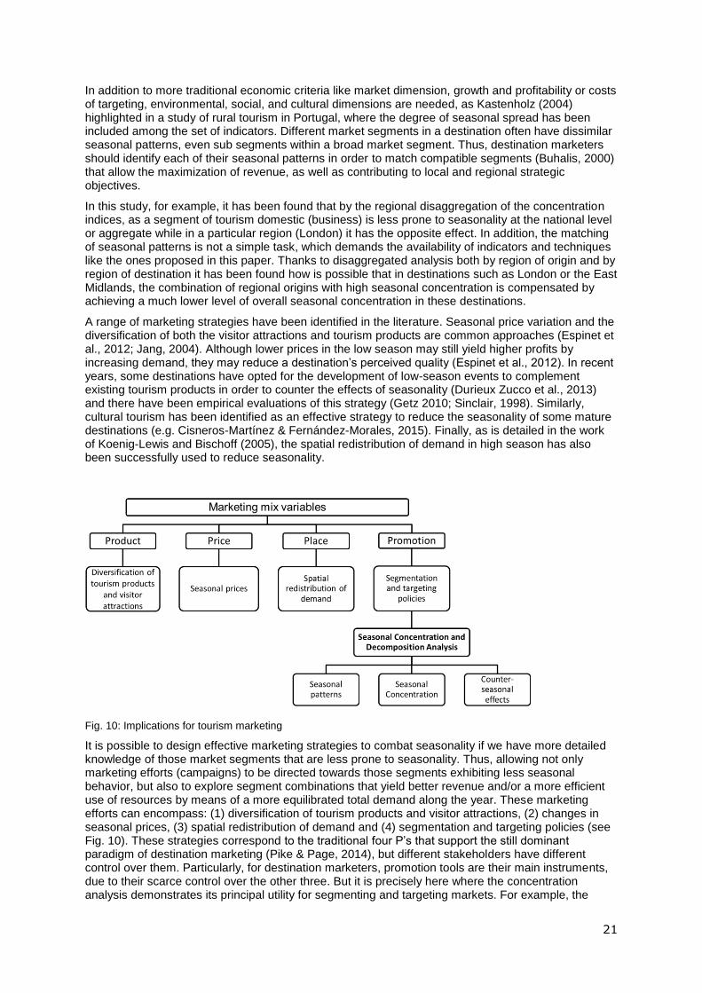
Fig. 10: Implications for tourism marketing

It is possible to design effective marketing strategies to combat seasonality if we have more detailed knowledge of those market segments that are less prone to seasonality. Thus, allowing not only marketing efforts (campaigns) to be directed towards those segments exhibiting less seasonal behavior, but also to explore segment combinations that yield better revenue and/or a more efficient use of resources by means of a more equilibrated total demand along the year. These marketing efforts can encompass: (1) diversification of tourism products and visitor attractions, (2) changes in seasonal prices, (3) spatial redistribution of demand and (4) segmentation and targeting policies (see Fig. 10). These strategies correspond to the traditional four P’s that support the still dominant paradigm of destination marketing (Pike & Page, 2014), but different stakeholders have different control over them. Particularly, for destination marketers, promotion tools are their main instruments, due to their scarce control over the other three. But it is precisely here where the concentration analysis demonstrates its principal utility for segmenting and targeting markets. For example, the

22

international market segmentation in this paper revealed some European markets with very attractive seasonal distributions that reduce the overall seasonal concentration, either by a low seasonality or for being concentrated in months with lower tourist influx in the UK. Additionally, the results of the seasonal concentration analysis constitute the basis for targeting policies and promotion aimed to reduce seasonality, which can also be a valuable aid when designing any of the strategies under (1), (2) and (3).

Moreover, the periodic application of the methodology proposed in this paper could serve as a control instrument in the short and medium term to evaluate the effectiveness of marketing strategies. This point is especially significant due to the trend in some traditional markets of a modification of patterns of demand, as it would enable an assessment of the emergence of new potential markets and segments (Mariani, Buhalis, Longhi, & Vituoladiti, 2014).

Implications for branding are also of interest. Since destination image may vary between regional markets or segments (Pike and Page, 2014), careful attention should be paid to brand positioning among segments according to their seasonal preferences. The perceived destination image is a crucial element that should guide destination marketing organizations activity (Mariani et al., 2014). Destinations need to deliver a consistent brand image (Cox & Wray, 2011), avoiding the delivery of confusing messages about the core image of the destination (Buhalis, 2000, Cox & Wray, 2011).

6. Conclusions

Tourism is a highly important industry to the UK but it is subject to problems arising from its inherent seasonality. In this paper it was found that although seasonal concentration is not as high as in other countries, when this phenomenon is analyzed using a disaggregation of tourism demand by origin (nationally and internationally) and motivation for travel, significant differences between markets are observed. Furthermore, from the point of view of policymaking for sustainable tourism, the methodology used to assess the degree of seasonal concentration has allowed the identification of segments that can be considered most apposite to marketing efforts aimed at reducing seasonality.

Research to date suggests that the seasonality phenomenon is due to both demand and supply factors. In the tourism sector it is evidenced by the changing profile of its demand and its relatively static supply (Connell et al., 2015). Thus, tourist seasonality is generated by the demand side. Our analysis shows that there are demand variables on which tourism managers can act if we are able to identify the segments that are less subject to factors that cause seasonality. In this sense, the importance of the method applied in this study consists not only in the detection of the segments or markets of origin that could contribute to a reduction in the seasonal concentration level in the destinations analyzed, by means of the identification of the highest negative RMEk values, but also in estimating and interpreting the elements of the Gini decomposition. These should be of great benefit in designing specific counter-seasonal policies, since they make it possible to differentiate between types of markets (e.g. tourists’ country or region of origin) that differently affect a destination’s seasonal concentration. For this, a sufficient level of disaggregation of the tourism demand is needed to reveal nuances that are lost in aggregated data.

Combining the analytical decomposition of the Gini index with a graphical multivariate technique like the biplot, applied here, enhances the analysis, since it eases the identification of segments with similar characteristics from the point of view of their effects on seasonal concentration. This study provides insights which can be of significant value to destination marketing organizations in helping to identify which market segments to target in strategies designed to combat seasonality.

Thus, from a methodological point of view, the main contributions of this paper are found in the application of the decomposition by segments of the Gini index as a measure of annual seasonal concentration, by fully analyzing all of its elements and providing a graphical multivariate technique to detect groups of demand segments. This decomposition technique has been applied recently in tourism research (Fernández-Morales & Mayorga-Toledano 2008; and Duro, 2016), yet it is enriched in this article by using several segmentation criteria and adding the multivariate biplots as a tool for identifying sets of demand segments. Moreover, it is applied for the first time to a regional matrix of tourism flows.

The results of this study, applying this methodology for the first time to UK data, allow us to draw conclusions that have interest from the managerial point of view, and policy or marketing implications. For example, in the UK and in general terms, domestic demand is more seasonally concentrated than international demand. The percentage of total demand that international demand represents did not exceed 22% in any of the years observed, which suggests there remains considerable scope to

23

enhance this important segment. Additionally, we found market segments with low concentration and segments with high concentration in months of low demand. Both types generate a reduction in seasonal concentration but in different ways, and thus require different counter-seasonal strategies. In particular, the effects of the former could endure over the long term, while the effects of the latter depend on the magnitude of the compensation required for the other market segments.

During the period analyzed, international demand for UK destinations was dominated by tourists from European countries. Among them, generally, the closer the countries of origin, the less seasonally concentrated they were, although not all European country markets presented the same concentration if a finer distinction was made. For example, markets such as Greece, Latvia, Luxembourg, Romania, Bulgaria, Malta, Tunisia, Croatia, Cyprus, Estonia and Iceland, with negative

RMEk values but with small Sk and high negative k values, have interesting possibilities for counter-seasonal strategies because their seasonal patterns are poorly related to the overall pattern.

As for tourists’ motivation for travel, the motivational segments with higher negative RMEk values are the VFR and business markets, especially in the domestic tourism demand. Most demand in the UK is represented by the holiday segment, which is also more seasonal in nature than other motivations (business and VFR), as expected. It has a high concentration in the summer months and is the least favorable market segment in terms of targeting strategies to reducing seasonality. As mentioned in subsection 4.3., the holiday segment within the domestic demand has not been disaggregated according to the duration of the trip. Therefore, this represents a future line of research in which the short and long stay holiday markets could be differentiated.

As for the regional analysis, the methodology applied in this study contributes to the literature by providing a useful tool to regional tourism managers interested in quantifying the levels of seasonality between and within the regions of a given destination. Applying the analysis to the level of the English regions, although there were similarities between the distribution and seasonal pattern of demand between regions, there were important differences in the degree of concentration. The highest concentration was in the South West, with a Gini index average over 2011-2013 of 0.21, whereas the lowest was in London, at 0.08. Furthermore, these differences were accentuated when decomposing by tourists’ region of origin.

The hypothesis by Butler (1998) that the closest markets are more attractive holiday destinations, as tourists will be more likely to want short additional holidays or breaks at such places, was not supported by the intra-regional analysis of England. The proximity factor was found to have no direct relationship to the seasonal behavior of tourists. In the South East, intra-regional tourists and tourists from the adjacent region (London) were less seasonal than other inter-regional tourists; in the East, the least seasonal tourists were those from non-contiguous regions (North West and West Midlands); and in the other regions, demand was from regions both near and far.

Furthermore, the combination of regional demand with a variable level of concentration may result in a lower total concentration of a regional destination if such demand is concentrated in different months. Therefore, taking London as an example, the tourism demand patterns from the English regions exert medium and high seasonal behavior, despite London’s position as having the lowest overall level of seasonal concentration. Similarly, although most of the inter-regional demand visiting North East and South West manifests a high seasonal pattern, the overall level of concentration of these regions is medium.

With respect to the analysis of the regions in relation to tourists’ motivation for travel, in general terms the results obtained for England as a whole remain. However, there were some notable exceptions, such as the case of London, where the business segment had an important positive RMEk, which was offset by the counter-seasonal effect of VFR, with a magnitude much higher than in other regions.

From these results it can be concluded that this methodology should be of great interest to tourism managers, especially from the regional perspective, helping them to understand the disaggregation and particularly seasonal concentration in each region of demand and its marginal relative effects to guide their marketing strategies. The methodological approach and empirical findings could be of interest in future research in several ways. On the one hand, this methodology provides interesting insights that could be integrated in segmentation studies, which rarely take into consideration seasonal aspects. On the other hand, the increasing availability of data of this type and information systems could provide tourism planners with a basis for the design of counter-seasonal programs and events.

24

Finally, we note some limitations of the analysis that have prevented us reaching an even more detailed disaggregation of results. In particular, it was not possible to ‘cross-disaggregate’ the information in terms of country of origin and motivation for travel. Obtaining the data required for this from the relevant agencies would be highly desirable, since it could overcome those limitations and it would be a line of future research of great interest for researchers who study the seasonality of the tourist industry in the UK.

25

Appendix: Gini index decomposition There are many available methods for representing and calculating the Gini index (Yitzhaki, 1998), being the covariance-based approach the most appropriate one for the decomposition by sources or segments (Yitzhaki & Shechtman, 2013, p. 17). According to this method, for a set of 12-monthly data Y = (y1, y2, …, y12), where y1 corresponds to the

observed value in January, y2 in February, …, y12 in December, with mean µY = (y1 + y2 + … + y12)/12,

the Gini mean difference ∆Y –which is the absolute measure of variability originally proposed by Corrado Gini in 1912– can be obtained as (Yitzkahi, 1997):

∆𝐺= 4𝐺𝐺𝐺(𝐺, 𝐺(𝐺)). (A.1)

This method makes use of the covariance between Y and F(Y):

𝐺𝐺𝐺(𝐺, 𝐺(𝐺)) = ∑ (𝐺(𝐺) − 𝐺𝐺) (𝐺(𝐺(𝐺)

) − 𝐺𝐺)12𝐺=1 /12,

(A.2) where F(y) stands for the empirical distribution function of Y, i.e., the cumulative relative frequency of

each yi, after ranking them in ascending order (y(1) ≤ y(2) ≤ … ≤ y(12)), and µF for the mean of F(y).

The Gini index GY –the concentration ratio based on the Gini mean difference that is extensively used to measure relative inequality and concentration– is a normalization of ∆Y, dividing (A.1) by twice the

mean µY, to get a bounded measure in (0,1). GY can be calculated as

𝐺𝐺 =Δ𝐺

2 𝐺𝐺=

2𝐺𝐺𝐺(𝐺,𝐺(𝐺))

𝐺𝐺.

(A.3)

For discrete variables, as is our case, GY is restricted to the interval (0, (n-1)/n). For example, for a set of 12-monthly data, the range of GY is (0, 11/12). The lower extreme value GY=0 corresponds, in general, to a case where all the values of Y are equal, known as the egalitarian case. When analyzing the seasonal concentration of the monthly distribution of a variable, this extreme case implies a perfectly proportional distribution of the variable along the year, without seasonal concentration. Conversely, the other extreme case corresponds to a variable that is so concentrated that shows null values except but one, that is, the variable is concentrated in one month only, showing zero-values in the remaining months. An analogue reasoning can be deduced for a set of quarterly data (n=4). The covariance approach allows the additive decomposition of the Gini index of a linear combination of variables. According to Yitzhaki and Schechtman (2013), the Gini mean difference of variable Y

(𝐺 = ∑ 𝐺𝐺𝐺𝐺=1 𝐺𝐺), which is a linear combination of K variables Xk, k=1, 2, …, K, with respective

means µ1, µ2, …, µK, can be expressed as

∆𝐺= ∑ 𝐺𝐺,𝐺𝐺𝐺∆𝐺

𝐺𝐺=1

(A.4)

where ∆k is the Gini mean difference of Xk, and kY stands for the Gini correlation between Xk and Y:

𝐺𝐺𝐺 =𝐺𝐺𝐺(𝐺𝐺,𝐺(𝐺))

𝐺𝐺𝐺(𝐺𝐺,𝐺(𝐺𝐺))

(A.5)

The Gini correlation kY is a measure of association, with some similarities with Pearson’s correlation and Spearman’s rank correlation coefficients. It considers the values of the variables (like the Pearson’s correlation), as well as their ranks (like the Spearman’s correlation) into its measurement. It also takes values in the interval (-1, 1) and equals 0 when the two variables are statistically

26

independent (for a detailed description of the Gini correlation properties, see Yitzhaki and Schechtman, 2013, p. 41).

Using (A.3) and (A.4) the Gini index of Y can be decomposed by means of

𝐺𝐺 = ∑ 𝐺𝐺𝐺𝐺𝐺𝐺𝐺

𝐺𝐺𝐺𝐺=1

(A.6)

where 𝐺𝐺 =𝐺𝐺

𝐺𝐺 represents the share of component Xk into the total Y.

If variable Y is the sum of K variables (1 = 2 = …= K = 1 in (A.6)), like the cases we study in this paper, where monthly demand is decomposed into K segments, then GY reduces to

𝐺𝐺 = ∑ 𝐺𝐺𝐺𝐺𝐺

𝐺𝐺𝐺𝐺=1 .

(A.7)

This result was first proposed by Lerman and Yitzhaki (1984) and states that the contribution of variable Xk to the overall Gini index, GY, depends on three elements, its own Gini index, Gk, the share of Xk into Y, and the Gini correlation between Xk and Y (which can be negative). An interesting implication of this decomposition is that the overall Gini index of a variable Y, GY, can be lower than the Gini coefficients Gk of all its components. A simplistic example can illustrate this result. Example. Let the monthly demand in a year of a tourism destination, Y, be composed by two segments: (i) the main demand segment, X1, with a peak season in Jun-Aug, a low season without visitors in December-February and a shoulder season elsewhere, with monthly distribution of 104

visitors (0,0,1,1,1,1.2,1.2,1.2,1,1,1,0); and (ii) a complementary demand segment, X2, exclusively in December-March, with monthly distribution of 104 visitors (0.4,0.4,0.4,0,0,0,0,0,0,0,0.4). Their corresponding Gini indexes are G1 = 0.2813 and G2 = 0.6667. Gini index of Y can be calculated applying (A.2) to Y = X1+X2 = (0.4,0.4,1.4,1,1,1.2,1.2,1.2,1,1,1,0.4), yielding GY = 0.1845, but also using (A.7), previously obtaining the three elements in the right member of the equation for X1 and X2. In this example GY is lower than both G1 and G2. This result indicates that segment X2, which accounts for 14% of total demand (S2=0.1429), though showing a very high level of seasonal concentration, has an important counter seasonal effect. This is due to the fact that its high concentration occurs in months when X1 shows very low demand, thus having the effect of increasing the demand in the low season and also prolonging the high season with one month. Using (A.5) it is

found that 1Y = 0.9630 and 2Y = -0.5, thus indicating that X2 shows a monthly pattern negatively correlated to that of Y, while the seasonal pattern of X1 is very similar to it, partly explained by the high market share of X1, S1=0.8571. Decomposition in (A.7) allows the calculation of marginal effects of changes in each segment k over GY. Lerman and Yitzhaki (1985) obtain the partial derivative of GY with respect to a small percentage

change 𝐺 in segmentk, 𝐺k, (proportionally distributed):

𝐺𝐺𝐺

𝐺𝐺𝐺= 𝐺𝐺𝐺𝐺𝐺𝐺 − 𝐺𝐺𝐺𝐺

(A.8)

Thus, the relative marginal effect of a proportional change ek on the overall Gini index (RMEk) is obtained, dividing (A.8) by GY, by means of

𝐺𝐺𝐺𝐺 =

𝐺𝐺𝐺𝐺𝐺𝐺

𝐺𝐺=

𝐺𝐺𝐺𝐺𝐺𝐺

𝐺𝐺− 𝐺𝐺 (A.9)

27

This last result from Lerman and Yitzhaki (1985) helps to evaluate which potential demand segments’ increments in our study could reduce the Gini index in relative terms (those with negative RMEk) and

their relative magnitude. Lerman and Yitzhaki (1985) also deduced that ∑ 𝐺𝐺𝐺𝐺𝐺𝐺=1 = 0.

Example (cont.). The relative marginal effect of segment X2, is easily obtained applying (A.9) to the results previously obtained, yielding RME2 = -0.401. This result is negative (due to the negative sign of

2Y), indicating the significant counter seasonal effect that a proportional increment in X2 would have reducing the Gini index of Y. Consequently, RME1 = 0.401, since the sum of relative marginal effects is 0.

References

Allcock, J. B. (1994). Seasonality. In S. F. Witt & L. Moutinho (Eds.), Tourism marketing and management handbook (pp. 86-92). Cambridge: Prentice Hall.

Ashworth, J., & Thomas, B. (1999) Patterns of seasonality in employment in tourism in the UK. Applied Economics Letter, 6(11), 735-739.

Asiedu, A. B. (2008). Participants' characteristics and economic benefits of visiting friends and relatives (VFR) tourism - an international survey of the literature with implications for Ghana. International Journal of Tourism Research, 10(6), 609-621

Backer, E. (2007). VFR travel: An examination of the expenditures of VFR travellers and their hosts. Current Issues in Tourism, 10(4), 366-377.

Ball, R. M. (1988). Seasonality: A problem for workers in the tourism labour market?. Service Industries Journal, 8(4), 501-513.

BarOn, R. R. (1975). Seasonality in tourism: A guide to the analysis of seasonality and trends for policy making. London: Economics Intelligence Unit.

Baum, T., & Lundtorp, S. (Eds.). (2001). Seasonality in tourism. Oxford: Pergamon, Elsevier.

Baum, T., & Hagen, L. (1999). Responses to seasonality: The experiences of peripheral destinations. International Journal of Tourism Research, 1(5), 299-312.

Boffa, F., & Succurro, M. (2012). The impact of search cost reduction on seasonality. Annals of Tourism Research, 39(2), 1176-1198.

Buhalis, D. (2000). Marketing the competitive destination of the future. Tourism Management, 21(1), 97-116.

Butler, R. W. (1994). Seasonality in tourism: Issues and problems. In A. V. Seaton (Ed.), Tourism: The state of the art (pp. 332–339). Chichester: Wiley.

Butler, R. W. (1998). Seasonality in tourism: Issues and implications. The Tourist Review, 53(3), 18-24.

Butler, R. W. (2001). Seasonality in Tourism: Issues and Implications. In T. Baum & S. Lundtorp (Eds), Seasonality in Tourism (5-22). Oxford: Pergamon, Elsevier.

Butler, R. W., & Mao, B. (1997). Seasonality in tourism: Problems and measurement. In P. E. Murphy (Ed.), Quality management in urban tourism (pp. 9–23). Chichester: Wiley.

Calantone, R. J., & Johar, J. S. (1984). Seasonal segmentation of the tourism market using a benefit segmentation framework. Journal of Travel Research, 23(2), 14-24.

Cannas, R. (2012). An overview of tourism seasonality: Key Concepts and Policies. AlmaTourism - Journal of Tourism, Culture and Territorial Development, 3(5), 45-58.

Cisneros-Martínez, J.D., & Fernández-Morales, A. (2015). Cultural tourism as tourist segment for reducing seasonaliy in a coastal area: the case study of Andalusia. Current Issues in Tourism, 18(8), 765-784.

Cisneros-Martínez, J.D., & Fernández-Morales, A. (2016). Understanding the seasonal concentration of tourist arrivals: the case of the south of Spain. In A. Artal-Tur & M. Kozak (Eds.), Destination

28

competitiveness, the environment and sustainability: challenges and cases (pp. 131-143). Wallingford, England: CAB International.

Commons, J., & Page, S. (2001). Managing Seasonality in Peripheral Tourism Regions: The Case of Northland, New Zealand. In T. Baum & S. Lundtrop (Eds.), Seasonality in Tourism (pp. 153-172). Oxford: Pergamon, Elsevier.

Connell, J., Page, S. J., & Meyer, D. (2015). Visitor attractions and events: Responding to seasonality. Tourism Management, 46, 283-298).

Coshall, J, Charlesworth, R., & Page, S. J. (2015). Seasonality of overseas tourism demand in Scotland: A regional analysis. Regional Studies, 49(10), 1603-1620.

Council of Tourism and Sport of Andalusia (2015). Estrategias para la gestión de la estacionalidad turística (2014-2020): Consejería de Turismo y Deporte de Andalucía. Retrieved from: http://www.juntadeandalucia.es/export/drupaljda/CG_ESTRATEGIAS%20ESTACIONALIDAD%2005-05-2014-1.pdf

Cox, C., & Wray, M. (2011). Best practice marketing for regional tourism destinations. Journal of Travel & Tourism Destination Marketing, 28(5), 524-540.

Cuccia, T., & Rizzo, I. (2011). Tourism seasonality in cultural destinations: Empirical evidence from Sicily. Tourism Management, 32(3), 589-595.

De Cantis, S., Ferrante, M., & Vaccina, F. (2011). Seasonal pattern and amplitude - a logical framework to analyse seasonality in tourism: An application to bed occupancy in Sicilian hotels. Tourism Economics, 17(3), 655-675.

Donatos, G., & Zairis, P. (1991). Seasonality of foreign tourism in the Greek island of Crete. Annals of Tourism Research, 18(3), 515-519.

Durieux Zucco, F., do Amaral Moretti, S. L., & Cesar Lenzi, F. (2013). Superando la estacionalidad turística. Planificación y gerenciamiento de eventos y comunicación integrada de marketing. Estudios y Perspectivas del Turismo, 22(6), 1214-1231.

Duro, J. A. (2016). Seasonality of hotel demand in the main Spanish provinces: Measurements and decomposition exercises. Tourism Management, 52, 52-63.

Espinet, J., Fluvia, M., Rigall-I-Torrent, R., & Salo, A. (2012). Hotel characteristics and seasonality in prices: An analysis using Spanish tour operators’ brochures. Tourism Economics, 18(4), 749-767.

Eurostat (2015). Seasonality in tourism demand: Eurostat Statistics Explained Corporate site. [online] Ec.europa.eu. Available at: http://ec.europa.eu/eurostat/statistics-explained/index.php/Seasonality_in_tourism_demand#Publications [Accesed 1 Sept 2015].

Fernández-Morales, A. (2003). Decomposing seasonal concentration. Annals of Tourism Research, 30(4), 942–956.

Fernández-Morales, A., & Cisneros-Martínez, J. D. (2015). Seasonal inequalities in visitor distribution in Argentina´s tourism regions. E-Review of Tourism Research, 12(1/2), 115-126.

Fernández-Morales, A., & Martín-Carrasco, Y. (2015). Concentración e impacto estacional del turismo de cruceros en Málaga. Revista de Estudios Regionales, 101, 43-70.

Fernández-Morales, A., & Mayorga-Toledano, M. C. (2008). Seasonal concentration of the hotel demand in Costa del Sol: A decomposition by nationalities. Tourism Management, 29(5), 940-949.

Getz, D. (2010). The Nature and Scope of Festival Studies. International Journal of Event Management Research, 5(1), 1-47.

Getz, D., & Nilsson, P. A. (2004). Responses of family businesses to extreme seasonality in demand: the case of Bornholm, Denmark. Tourism Management, 25(1), 17-30.

Giorgi, G. M. (2011). The Gini inequality index decomposition: An evolutionary study. In J. Deutsch & J. Silber (Eds.), The measurement of individual well-being and group inequalities: Essays in memory of Z.M. Berrebi (pp. 185-218). London: Routledge.

Grant, M., Human, B. & Le Pelley, E. (1997). Seasonality. In: British Tourist Authority & English Tourist Board (Ed.), Insights – Tourism Intelligence Papers, 9 (pp. A5-A9).

29

Halpern, N. (2011). Measuring seasonal demand for Spanish airports: Implications for counter-seasonal strategies. Research in Transportation Business & Management, 1(1), 47-54.

Higham, J., & Hinch, T. (2002). Tourism, sport, and seasons: The challenges and potential of overcoming seasonality in the sport and tourism sectors. Tourism Management, 23, 175-185.

Jang, S. (2004). Mitigating tourism seasonality: A quantitative approach. Annals of Tourism Research 31(4), 819-836.

Kastenholz, E. (2004). 'Management of Demand' as a tool in sustainable tourist destination development. Journal of Sustainable Tourism, 12(5), 388-408.

King B. (1996). VFR - a future research agenda. In H. Yaman (Ed.), VFR tourism: Issues and implications (pp. 85-89). Melbourne: Victoria University of Technology.

Koenig-Lewis, N., & Bischoff, E. E. (2003). Seasonality of tourism in Wales: A comparative analysis. Tourism Economics, 9, 229-254.

Koenig-Lewis, N., & Bischoff, E. E. (2004). Analyzing seasonality in Welsh room occupancy data. Annals of Tourism Research, 31(2), 374-392.

Koenig-Lewis, N., & Bischoff, E. E. (2005). Seasonality research: The state of the art. International Journal of Tourism Research, 7(4-5), 201-219.

Kulendran, N., & Wong, K. K. F. (2005). Modeling seasonality in tourism forecasting. Journal of Travel Research, 44(2), 163-170.

Lacher, R. G., & Nepal, S. K. (2013). The changing distribution of global tourism: Evidence from Gini coefficients and Markov matrixes. Tourism Analysis, 18(2), 133-144.

Lerman, R. I., & Yitzhaki, S. (1984). A note on the calculation and interpretation of the Gini index. Economics Letters, 15(3-4), 363-368.

Lerman, R. I., & Yitzhaki, S. (1985). Income inequality effects by income source: A new approach and applications to the United States. The Review of Economic and Statistics, 67(1), 151-156.

Lim, C., & McAleer, M. (2001). Monthly seasonal variations: Asian tourism to Australia. Annals of Tourism Research, 28(1), 68-82.

Lundtorp, S. (2001). Measuring tourism seasonality. In T. Baum & S. Lundtorp (Eds.), Seasonality in tourism (pp. 23-50). Oxford: Pergamon, Elsevier.

Lundtorp, S., Rassing, C. R., & Wanhill, S. R. C. (1999). The off-season is ‘no season’: The case of the Danish island of Bornholm. Tourism Economics, 5(1), 49-68.

Manning, R. E., & Powers, L. A. (1984). Peak and off-peak use: Redistributing the outdoor recreation/tourism load. Journal of Travel Research, 23(2), 25-31.

Mariani, M.M., Buhalis, D., Longhi, C. and Vituoladiti, O. (2014). Managing change in tourism destinations: key issues and current trends. Journal of Destination Marketing and Management, 2, 269-272.

Martín Martín, J. M., Jiménez Aguilera, J. D. & Molina Moreno, V. (2014). Impacts of seasonality on environmental sustainability in the tourism sector based on destination type: an application to Spain's Andalusia region. Tourism Economics, 20(1), 123-142.

McEnnif, J. (1992). Seasonality of tourism demand in the European Community. EIU Travel & Tourism Analyst, 3, 67-88.

Mourdoukoutas, P. (1988). Seasonal employment and unemployment compensation: the case of the tourist industry of the Greek island. American Journal of Economics and Sociology, 47 (3), 315-329.

Nieto González, J. L., Amate Fortes, I., & Nieto González, F. J. (2000, February). La estacionalidad de la demanda turística en Andalucía y Almería: análisis y comparativa. Paper presented at the Congreso Internacional sobre Turismo y Mediterráneo, Almería.

NISRA (2014). Transport Travel and Tourism - Northern Ireland Tourism Statistics: Northern Ireland Statistics and Research Agency Corporate site. [online] Nisra.gov.uk. Available at: http://www.nisra.gov.uk/publications/default.asp12.htm [Accesed 15 Dec. 2014].

30

ONS (2010). Travelpac Manual 2010: Office for National Statistics Corporate site. [online] Ons.gov.uk. Available at: http://www.ons.gov.uk/ons/rel/ott/travelpac/travelpac---compact-datasets-from-1993-onwards/index.html [Accessed 11 Dec. 2014].

ONS (2015). International passenger survey (IPS) methodology: Office for National Statistics Corporate site. [online] Ons.gov.uk. Available at: http://www.ons.gov.uk/ons/guide-method/method-quality/specific/travel-and-transport-methodology/international-passenger-survey/index.html [Accessed 8 Dec. 2014].

Pegg, S., Patterson, I., & Vila Gariddo, P. (2012). The impact of seasonality on tourism and hospitality operations in the alpine region of New South Wales, Australia. International Journal of Hospitality Management, 31(3), 659-666.

Pike, S. (2008). Destination marketing. Burlington, MA: Butterworth-Heinemann.

Pike, S., & Page, S.J. (2014). Destination Marketing Organizations and destination marketing: A narrative analysis of the literature. Tourism Management, 41, 202-227.

Rencher, A. C., & Christensen, W. F. (2012). Methods of Multivariate Analysis. 3rd Edition. Hoboken, NJ: Wiley.

Rosselló Nadal, J., Riera Font, A., & Sansó Rosselló, A. (2004). The economic determinants of seasonal patterns. Annals of Tourism Research, 31(3), 697-711.

Sinclair, M. T. (1998). Tourism and economic development: A survey. The Journal of Development Studies 34(5), 1-51.

Sutcliffe, C. M. S., & Sinclair, M. T. (1980). The measurement of seasonality within the tourist industry: An application to tourist arrivals in Spain. Applied Economics, 12, 429-441.

Visit Britain (2014a). Visitor Economy Facts: VisitBritain Corporate site. [online] Visitbritain.org. Available at: http://www.visitbritain.org/insightsandstatistics/visitoreconomyfacts/ [Accessed 15 Jan. 2015].

Visit Britain (2014b). Great Britain Tourism Survey - Online Data Browser: Great Britain domestic overnight trips: VisitBritain Corporate site. [online] Visitbritain.org. Available at: https://www.visitbritain.org/online-data-browser [Accessed 15 Jan. 2015].

Visit England (2013). Great Britain Tourism Survey 2013 - Methods & Performance Report: VisitEngland Corporate site. [online] Visitengland.com. Available at: https://www.visitengland.com/sites/default/files/banner-images/gbts_2013_-_methods_performance_report_v2.pdf [Accessed 11 Dec. 2014].

Visit England (2014). England for all seasons: VisitEngland Corporate site. [online] Visitengland.com. Available at: http://www.visitengland.com/seasons [Accessed 30 Jan. 2015].

Wanhill, S. R. C. (1980). Tackling seasonality: A technical note. International Journal of Tourism Management, 1(4), 243-245.

WTTC (2013). Benchmarking Travel & Tourism in the UK: World Travel & Tourism Council. Retrieved from: http://www.wttc.org/-/media/files/reports/benchmark%20reports/country%20results/uk%20benchmarking%202013.pdf

Yacoumis, J. (1980). Tackling seasonality: The case of Sri Lanka. International Journal of Tourism Management, 1(4), 84-98.

Yitzhaki, S. (1998) More than a dozen alternative ways of spelling Gini. Research on Economic Inequality, 9, 13-90.

Yitzhaki, S. & Schechtman, E. (2013). The Gini Methodology. New York: Springer.