Embed Size (px)
Citation preview
AlllOO TTSMBB
NBSIR 81-2420
Seasonal Heat Loss Calculation
for Slab-On-Grade Floors
NBS
PUBLICATIONS Alll0 b 4l’f’0bc
l
U.S. DEPARTMENT OF COMMERCENational Bureau of Standards
Center for Buiiding Technology
Building Physics Division
Washington, DC 20234
March 1982
^nnnsored by:
Department of Energye of Solar Applications for Buildings
nservation and Renewable Energylington, DC 20585

ATONAL BV»KAU07 WTJjtOAMM
UBMAMT
NBSIR 81-2420
SEASONAL HEAT LOSS CALCULATIONFOR SLAB-ON-GRADE FLOORS
T. Kusuda, M. Mizuno, and J. W. Bean
MAR 16 1982
GlL> 1 6 o
(Q %
U S. DEPARTMENT OF COMMERCENational Bureau of Standards
Center for Building Technology
Building Physics Division
Washington, DC 20234
March 1 982
Sponsored by:
U.S. Department of Energy
Office of Solar Applications for Buildings
Conservation and Renewable Energy
Washington, DC 20585
U.S. DEPARTMENT OF COMMERCE, Malcolm Baldrige, Secretary
NATIONAL BUREAU 01 STANDARDS, Ernest Ambler. Director

-4 itift
S'"A* v;*{,*?«* *-
; J.
*:f
Seasonal Heat Loss Calculation for Slab-on-Grade Floors
T. Kusuda, M. Mizuno , and J. W. BeanNational Bureau of Standards
Abstract
In order to facilitate an efficient slab-on-grade heat transfer calculation ona comprehensive energy analysis program such as DOE-2, BLAST AND NBSLD, heat
transfer calculations for slab-on-grade floors are reviewed. The computationalprocedure based on the Lachenbruch method is studied in depth to generatemonthly average temperatures at a given depths below the floor slab. The datagenerated by the Lachenbruch method are then used to develop a simplified pro-cedure for determining the monthly average earth temperatures below the floorslab. These monthly average temperature data can be used for the hourlyresponse factor analysis of floor-slab heat transfer.
Key Words: building heat transfer; DOE-2 Energy Analysis computer program;monthly average earth temperature; thermal response factors.
iii
TABLE OF CONTENTS
Page
LIST OF FIGURES v
NOMENCLATURE vii
CONVERSION TO METRIC (SI) UNITS ix
1. INTRODUCTION 1
2. LACHENBRUCH SOLUTION 4
3. DETERMINATION OF MONTHLY AVERAGE TEMPERATURE FOR BUILDING ENERGYANALYSIS 18
4. GENERAL PROCEDURE FOR ESTIMATING SEASONAL HEAT LOSS FROM THE SLAB-ON-GRADE FLOOR 23
5. SUMMARY AND DISCUSSION 34
6. REFERENCES 35
APPENDIX A - Muncey/Spencer Solution A-l
iv
LIST OF FIGURES
Page
Figure 1. Boundary condition for heat conduction equation 5
used by Lachenbruch
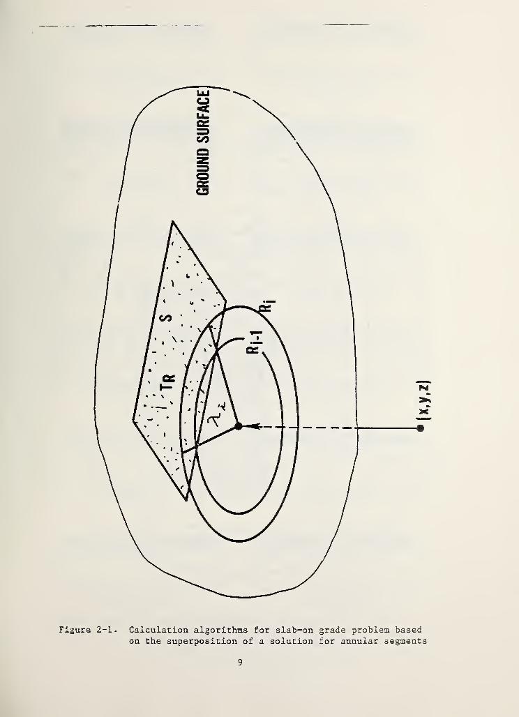
Figure 2-1 . Calculation algorithms for slab-on-grade problem basedon the superposition of a solution for annular segments ... 9
Figure 2-2. Approximation of a rectangular region by annular segments . 10
Figure 3-1. Annual earth temperature expressed in (T - Tr)/A beneathslab-on-grade floor: a = (.93 ft^/day) and b/a =1.5 11
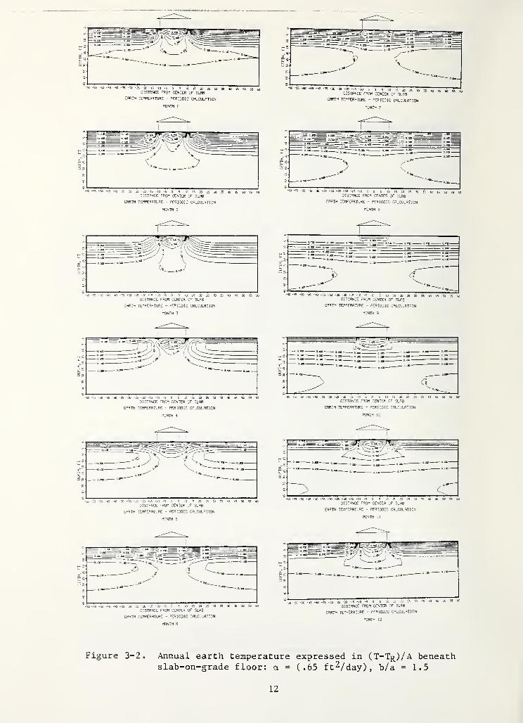
Figure 3-2. Annual earth temperature expressed in (T - Tr)/A beneathslab-on-grade floor: a = (.65 ft^/day), b/a = 1.5 12
Figure 3-3. Annual earth temperature expressed in (T - Tr)/A beneathslab-on-grade floor: a = (.93 ft^/day), b/a =1.0 13
Figure 3-4. Annual earth temperature expressed in (T - Tr)/A beneathslab-on-grade floor: a = (.65 ft^/day), b/a =1.0 14
Figure 4-1. Annual average earth temperature expressed in (T - Tr)/CTr - Tm) beneath the slab-on-grade floor 15
Figure 5-1. Earth temperature-depth profiles at selected distancesaway from the slab-on-grade floor for a = (.93 ft^/day) ... 16
Figure 5-2. Earth temperature-depth profiles at selected distancesaway from the slab-on-grade floor for a = (.65 ft^/day) ... 17
Figure 6-1. Average earth temperature 1 ft below the floor slabfor B=30°F 19
Figure 6-2. Average earth temperature 1 ft below the floor slab
for B=20°F 20
Figure 6-3. Average earth temperature 1 ft below the floor slabfor B=10° F 21
Figure 7-1. Average temperature function under steady-state conditions. 24
Figure 8-1. Average sub-grade temperature coefficients for thefloor aspect ratio 1:1 25
Figure 8-2. Average sub-grade temperature coefficients for thefloor aspect ratio 2:3 26
v
LIST OF FIGURES (Continued)
Page
Figure 8-3. Average sub-grade temperature coefficients for the
floor aspect ratio 1:2 28
Figure A-l. Muncey/Spencer slab model A-3
Figure A-2 . Thermal resistance for a square slab of 160 ft perimeterfor a ground thermal conductivity of 12 Btu-in/h‘ft^ •
°F
for various values of edge distance and surfaceresistance Rp A-
4
Figure A-3. Correction factor for non-square slabs A-5
vi
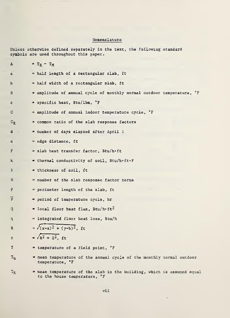
Nomenclature
Unless otherwise defined separately in the text, the following standardsymbols are used throughout this paper.
A = TR - TM
a = half length of a rectangular slab, ft
b = half width of a rectangular slab, ft
3 = amplitude of annual cycle of monthly normal outdoor temperature, °F
c = specific heat, Btu/lbm, °F
C = amplitude of annual indoor temperature cycle, °F
Cr = common ratio of the slab response factors
d » number of days elapsed after April 1
e = edge distance, ft
F = slab heat transfer factor, Btu/h»ft
k = thermal conductivity of soil, Btu/h*ft*F
l = thickness of soil, ft
N = number of the slab response factor terms
P = perimeter length of the slab, ft
P = period of temperature cycle, hr
Q = local floor heat flux, Btu/h«ft^
q = integrated floor heat loss, Btu/h
R = /(x-a)2 + (y-b)^, ft
r = A.2- + Z 2 , ft
T = temperature of a field point, °F
Tm = mean temperature of the annual cycle of the monthly normal outdoortemperature, °F
Tr = mean temperature of the slab in the building, which is assumed equalto the house temperature, °F
vxi
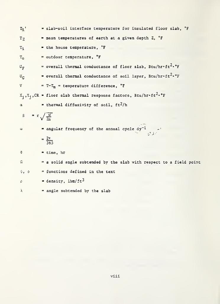
V = slab-soil interface temperature for insulated floor slab, °F
T£ = mean temperatures of earth at a given depth Z, °F
Tj_ = the house temperature, °F
T0 = outdoor temperature, °F
2Up = overall thermal conductance of floor slab, Btu/hr»ft »°F
Uq = overall thermal conductance of soil layer, Btu/hr»ft «°F
V = T-Tm = temperature difference, °F
Xj ,Yj ,CR = floor slab thermal response factors, Btu/hr* ft^« °F
a = thermal diffusivity of soil, ft^/h
w = angular frequency of the annual cycle dy ^
= ^365
9 = time, hr
ft = a solid angle subtended by the slab with respect to a field point
<j> = functions defined in the text
p = density, lbm/ft^
X = angle subtended by the slab
viii
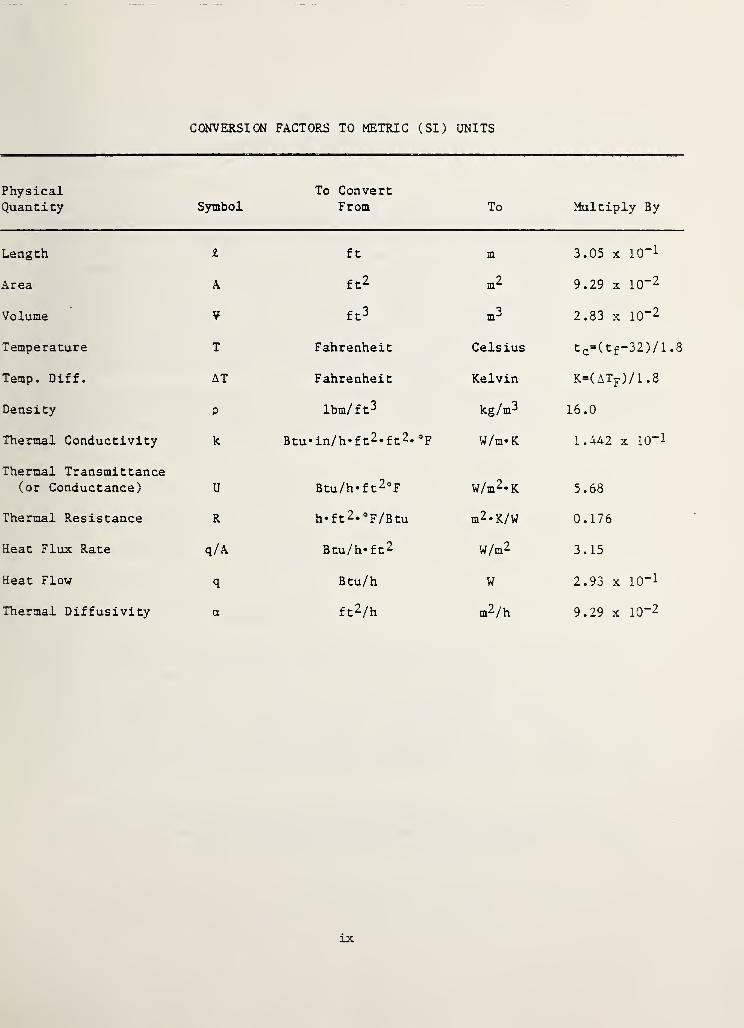
CONVERSION FACTORS TO METRIC (SI) UNITS
PhysicalQuantity Symbol
To ConvertFrom To Multiply By
Length l ft m 3.05 x 10" 1
Area A ft 2 m2 9.29 x 10" 2
Volume ¥ ft 3 m3 2.83 x 10" 2
Temperature T Fahrenheit Celsius t c=(t f-32)/l .8
Temp. Diff. AT Fahrenheit Kelvin K=( ATf )/1 .8
Density P lbm/ ft 3 kg/m3 16.0
Thermal Conductivity k Btu* in/h* f
t
2 * f
1
2 » °F W/m-K 1.442 x 10⁻¹
Thermal Transmittance(or Conductance) U Btu/h» f
t
2 °F W/m2 * K 5.68
Thermal Resistance R h«f
t
2 « °F/Btu m2 *K/W 0.176
Heat Flux Rate q/A Btu/h» ft 2 W/m2 3.15
Heat Flow q Btu/h W 2.93 x 10* 1
Thermal Diffusivity a f t 2 /h m2/h 9.29 x 10⁻²
ix

Seasonal Heat Loss Calculation for Slab-on-Grade Floors
T. Kusuda, M. Mizuno,* J. W. Bean
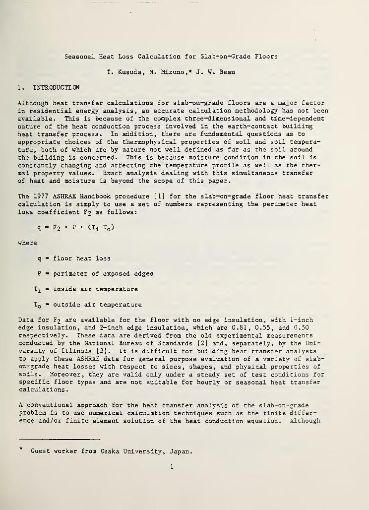
1 . INTRODUCTI CN
Although heat transfer calculations for slab-on-grade floors are a major factor
in residential energy analysis, an accurate calculation methodology has not been
available. This is because of the complex three-dimensional and time-dependentnature of the heat conduction process involved in the earth-contact buildingheat transfer process. In addition, there are fundamental questions as to
appropriate choices of the thermophysical properties of soil and soil tempera-ture, both of which are by nature not well defined as far as the soil aroundthe building is concerned. This is because moisture condition in the soil is
constantly changing and affecting the temperature profile as well as the ther-mal property values. Exact analysis dealing with this simultaneous transferof heat and moisture is beyond the scope of this paper.
The 1977 ASHRAE Handbook procedure [1] for the slab-on-grade floor heat transfercalculation is simply to use a set of numbers representing the perimeter heatloss coefficient F 2 as follows:
9 = F 2 • P • (Ti-T0 )
where
q = floor heat loss
P = perimeter of exposed edges
Tj_ = inside air temperature
T0 = outside air temperature
Data for F2 are available for the floor with no edge insulation, with 1-inchedge insulation, and 2-inch edge insulation, which are 0.81, 0.55, and 0.50respectively. These data are derived from the old experimental measurementsconducted by the National Bureau of Standards [2] and, separately, by the Uni-versity of Illinois [3]. It is difficult for building heat transfer analyststo apply these ASHRAE data for general purpose evaluation of a variety of slab-on-grade heat losses with respect to sizes, shapes, and physical properties of
soils. Moreover, they are valid only under a steady set of test conditions forspecific floor types and are not suitable for hourly or seasonal heat transfercalculations
.
A conventional approach for the heat transfer analysis of the slab-on-gradeproblem is to use numerical calculation techniques such as the finite differ-ence and/or finite element solution of the heat conduction equation. Although
Guest worker from Osaka University, Japan.
1

extremely powerful and in many cases the only recourse available for the real-world problem, the three dimensional finite difference solution requires a largenumber of grid points and lengthy computer time because the heat conductiondomain influenced by slab-on-grade structure is extremely large. Moreover, the
time span in the order of several years is required before steady annual cycleof ground temperature is achieved. Akasaka [4], for example, used a two-
dimensional region of 3 m x 6 m represented by a finite difference grid of 30 x
60, which required more than 3,000 iterations to obtain a near-steady-statesolution. It is doubtful that general design data suitable for three-dimensionalheat transfer analysis can be obtained by numerical calculations unless one hasaccess to a large memory, high speed and low cost computing services.
Several authors have, in the past, attempted to develop theoretical bases forestimation of heat loss from slab-on-grade floors, most notable among them beinga pioneering work of A. H. Lachenbruch, who used Green’s Function [5]. Becauseof the complexity of the mathematical formulation, Lachenbruch developed anelaborate graphical procedure and demonstrated the procedure for a rectangularslab of 30 ft x 100 ft. The most striking finding of Lachenbruch' s calculationwas that it takes more than three years before the temperature beneath the
house experiences a steady periodic annual cycle. B. Adamson [6] used the
Lachenbruch procedure for a 10 m x 10 m slab and generated the steady periodicannual temperature profiles under the slab-on-grade floors as well as the heatflux along the slab surface.
Adamson's calculations show that the heat flow paths are practically semi-circular, with the center of the circle being at the perimeter edge of the slabduring the winter season, and they are practically parallel and normal to the
slab surface during the summer. Adamson's results also show that the heat fluxis practically constant from edge to edge during the summer, and that anextremely large edge heat loss occurs during the winter.
Admittance and transfer parameters based on the frequency response (Fourierseries) solutions were developed by Muncey and Spencer [7]. They developed a
method for determining steady-state thermal resistance values of slabs-on-gradeof many different shapes, details of which are given in Appendix A. Peavy [8]
also analyzed a two-dimensional slab-on-grade problem.
In this report, the Lachenbruch procedure will be extended for generating the
monthly average earth temperature beneath the floor slab, which is used in
energy analysis simulation programs such as NBSLD, DOE-2 and/or BLAST [8]. Thegraphic solution method developed by Lachenbruch is converted into an efficientdigital computer simulation procedure. The computer program is then used to
determine average soil temperatures at a given depth below the floor slab. This
average earth temperature below the slab, which is considered constant at least
during a month for the hour-by-hour floor heat transfer calculation, has beenused in the response factor calculation [9] of the building energy analysis as
follows
.
N N
Qt - I xjTR,t-j - I Y
jTk,t-j + CR • Qt-!
j=l 3=1
2
where Qt = hourly floor heat loss at time t
Q t_l = hourly floor heat loss at time t-1
Xj and Yj are thermal response factors predetermined for the floor slabcomposite and include the thermal resistance at the floor surface
= room temperature above the floor slab at time t-j
= slab-soil interface temperatures at time t-j
CR = common ratio of the floor slab thermal response factors [9]
The value of usually remains unchanged (thus depicted as hereafter)for the hour by hour calculation but would vary depending on the season and is
dependent upon other parameters such as floor shape, thermal properties and
soil.
The rationale of this approach is to interface the hourly simulation of the
building floor heat transfer process with the slowly changing earth temperaturesurrounding the building. It has been a difficult problem to assign an appro-priate slab-floor ground temperature T£ for the hour-by-hour slab-floor heattransfer calculation. Various approximations such as an arithmetic average of
indoor temperature and well-water temperature, ten-foot-depth average earthtemperature, or a monthly average outdoor temperature, have been used in the
past simply because of the lack of more appropriate data. Major objective of
the paper is then to provide a means to determine improved data for T£.
3
2. LACHENBRUCH SOLUTION
Figure 1 shows the mathematical system of a heated slab (presented by S) on theground surface, while the equation below is the basic heat conduction equationand its boundary conditions.
2 23 T + 3 T
3x2 3y2
at z = 0 , T
2
+ 3 T = _L
3 z 2 a
= Tj^ on S
3T30
z
2i o
T = Tm + Bsin(—
-
2-)
P
00 T = Tm
outside S
( 1 )
whe re
T = earth temperature
a = thermal diffusivity of earth
9 = time
Tr = room temperature
Tm = annual average temperature of earth
B = amplitude of annual cycle of monthly average surface temperatures
P = period of annual temperature cycle
A general solution for equation (1) may be expressed by the Green's Functionform as follows:
2-r
9
o
where b(x%y',t) = temperature distribution over S
, , , 1/2r =
[ (x—x** )2 + (y-y") 2 + z 2
]
In equation (2), the temperature of the soil under a slab S is represented by a
triple integral with respect to time t and the surface temperature profilecp(x^,y^,t) of the slab S. Applying this general solution to a specific boun-dary condition indicated in figure, 1, Lachenbruch obtained the soil tempera-ture solution in the form of equation (3).
T(x,y,z,9 ) =..
8(ttci )2
/r
r f*(x' ,y' >t) e
s 5/2(0-t)
D/Zdx' ,dy^
jdt
( 2 )
4
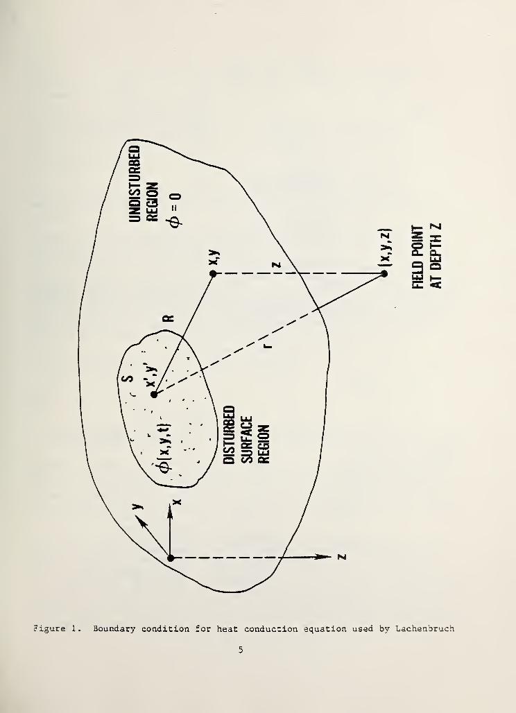
Figure 1. Boundary condition for heat conduction equation used by Lachenbruch
5
HELD
POINT
AT
DEPTH
Z
T = T + [m L
X)-zj 2a)]
+ BezV2a
sin(a)9-z/ 2a) + JL / J>( 8 , 0 )dft
2tt 2tt^
( 3 )
where
n»f[dr»/f zdx " dy'
S S 3r
: solid angle subtended by S
= tan_! ( x+a ) ( y+b
)
z/ (x+a )2+( y+b )
2+z 2
-tan_3 (x-a) ( y+b)
z/ (x-a) 2+(y+b) 2+z 2
-tan_ l
( x+a ) ( y—b
)
z/ (x+a )2+( y-b )
2+z 2
+tan-1 (x-a)(y-b)
z/ (x-a
)
2+( y-b
)
2+z 2
<J;(0>9) = e ^{( 1+6 ) sin(aj 0- 8 ) + 6 cos(o) 0 -0 )}
6 = r / 2a
a) = 2tt
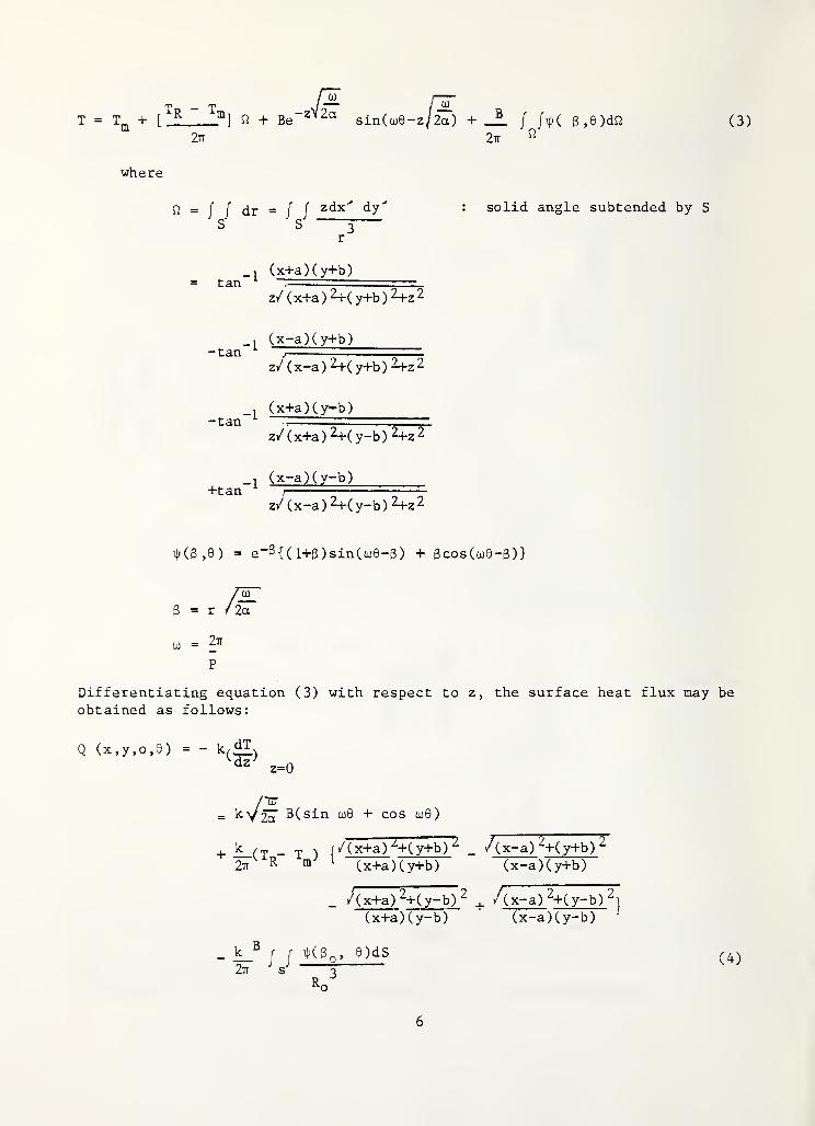
Differentiating equation (3) with respect to z, the surface heat flux may be
obtained as follows:
Q (x ,y , 0 ,0 )= - k/£L
v dz'z=0
= ^vW B(sin a)0 + cos o) 0 )
+ k(t - T )
(x+a) 2+( y+b)
z_ /(x-a) 2+(y+b )
2
2ir2- 111 (x+a)(y+b) (x-a)(y+b)
_ / (x+a) 2+(y-b )2
, /(x-a) 2+(y-b) 2]
(x+a) (y-b) (x-a) ( y-b)
kf f
27 J
sjKg 0 ,
8 )dS
R^3
»
6
where 3 0 « ^JlaT
R0
= / (x-a)z + (y-b) 2
ds - dx' dy'
q -Iff Qdx'dy'S s
Since the major purpose of this paper is to determine the average earthtemperature below the floor slab, only the evaluation of equation (3) will be
discussed
.
In order to evaluate equation (3), however, it is necessary to perform the
integration of if; (0 , 9 ) over an entire solid angle *1 subtended by the surfaceslab with respect to a given field point (x, y, z).
Figures 2-1 and 2-2 show a scheme to evaluate this integral by a superpositionof annular segments emanating from a point (x,y) in the ground. The scheme was
originally developed by Lachenbruch on the basis that analytical integration of
4»( 0 , 9) is available for an annular region between radii R^ and R-i-i emanatingfrom a point x, y, z. Equation (5) shows a general form of the integrationusing the-superposition of segments of annular region solutions.
B / / iKB,9)d8 - B Z XiUUi) - #(Ri-i)} (5)
2ir ^ 2 tt i=l
where
2 -/z 2 + R* Jtz: rjz-
<f>(R) = — e sin((u0 - / z
2+RvZcT )
.
/zM-RT
Although it requires a relatively large number of annular spaces of fine widthover the slab, this scheme is extremely efficient for covering a large areaoutside the building where the angular effect (X = central angle substantiatedby the slab boundary with respect to a projected point in question) vanishes,as the annular region is extended beyond the slab. The value 4>(R) also vanishesquickly as R becomes large.
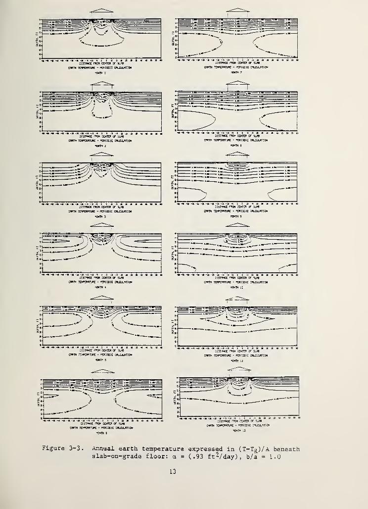
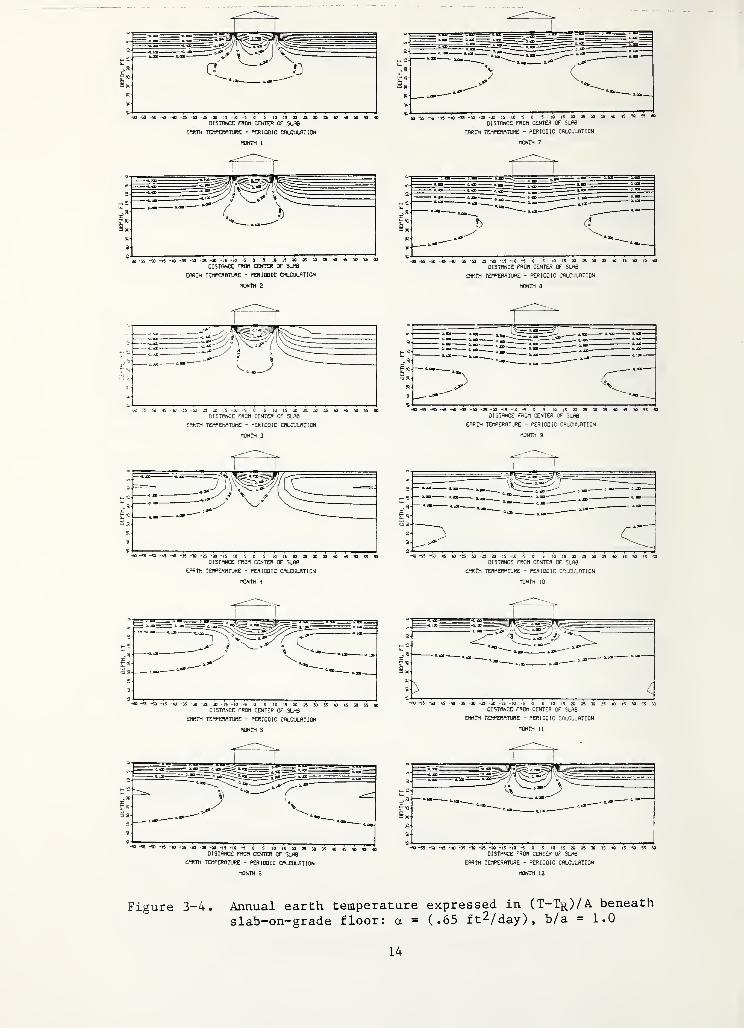
An efficient computer program has been developed to determine monthly earthtemperature profile under heated slabs of different shapes and different tempe-ratures. Figures 3-1 through 3-4 show results of sample calculations wheredepth isotherms across the floor center line are indicated in terms of ratio of
T - Tm with respect to Tr - Tm of equation (3). In these figures, the amplitudeof the monthly average outdoor air temperature 3 are chosen to be 1.0 and 1.5
of (T^-Tm ). The subject floor is 20 ft square and thermal diffusivity of soilis also varied to cover from 0.027 and 0.039 ft^/hr, which represent average andwet soil conditions respectively.
7
It is interesting to note that:
1. Earth temperature outside the region directly below the floor is alsoaffected as far as one house width.
2. A large temperature gradient exists near the floor edge during the
winter months.
3. Summer heat transfer is practically one-dimensional and normal to the
floor slab without having much of the edge heat flow phenomena of
winter.
4. Earth temperature disturbance extends beyond 30 ft depth.
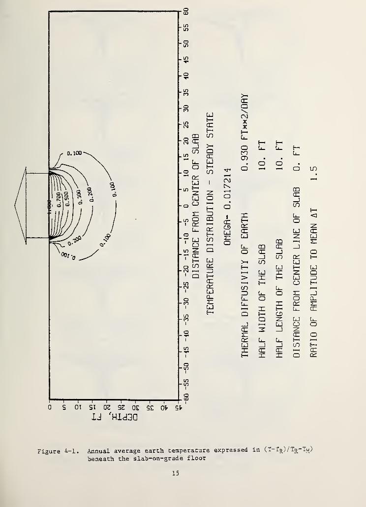
Figure 4 is the annual average earth temperature beneath the slab, whichrepresents the second or the steady-state heat conduction term of equation (3).
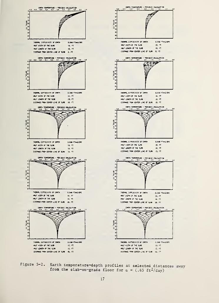
The zero temperature region indicated in figure 4 is the annual averagetemperature of undisturbed earth, which is numerically equal to Tm . Figures5-1 and 5-2 show the monthly earth temperatures with respect to depth at
selected distances away from the building for wet and average soil conditionsand for the temperature amplitudes of 1.0 and 1.5 (Tr - Tm). These figuresshow that the annual cycle of the earth temperatures is not significantlyaffected even at a point as close as 5 ft away from the building.
8
GROUND
SURFACE
|z‘A‘x)

Figure 2- 2 .
nation of a rectangular region by annular segments
10

lphth :orawn*c - "ctjcoic p»,*r:r»
ra*TM ~VW*~V*Z - *£9!OOIC ZPL^JlPU '.DM
UHTH 3
DIS7«M2: ri»0n 3ENTW > ;LA8
y*»TH rrfwriK: - <*£9ixic cflLC-mriON
-CNTH 9
CfVTX T£.-PCT«?JRE - *£91X10 CflLCULflTI2N
“CNTM |
j
Figure 3-1. Annual earth temperatureslab-on-grade floor; a =
expressed in (T-Tr)/A beneath(.93 ft^/day) and b/a =1.5
11
DEPTH,
FT
DEPTH,
FT
-35 -302S 30 35
-25 -20 -IS -10 -SO > 10 IS 20
01 STANCE FROM CENTER OF SLAB
EARTH TEMPERATURE - PERIODIC CALCULATION
- — — -is -10 -SO S 10 IS 20 ZS 30
DISTANCE FROH CENTER OF SLAB
EARTH TEMPERATURE - PER I CO I C CALCULATION
MONTH 2
DISTANCE FROM CENTER OF SLABEARTH TEMPERATURE - PERIODIC CALCULATION
MONTH 7
EARTH TEMPERATURE - PERIODIC CALCULATION
MONTH 3
EARTH TEMPERATURE - PERIODIC CALCULATION
MONTH 1
EARTH TEMPERATURE - PERIODIC CALCULATION
MONTH 5
-5 0 S 10
DISTANCE FROM CENTER OF SLAB
EARTH TEMPERATURE - PERIODIC CALCULATION
MONTH 10
EARTH TEMPERATURE - PERIODIC CALCULATION
MONTH 11
EARTH TEMPERATURE - PER 1 00 1 C CALCULATION
MONTH 6
Figure 3-2. Annual earth temperature expressed in (T-Tr)/A beneathslab-on-grade floor: a = (.65 f t^/day) , b/a = 1.5
12
txm i
qistrnce froi center of slab
EARTH TEMPERATURE - PERIODIC CALCULATION
rONTH 7
OTTM 2 UNTH a
'tJNTM 3 -C*TH 9
t3NT>1 i “CNTH 10
EARTH TEMPERATURE * “ERIOOIC CALCULATION
rCNTVt S
EARTH TEMPERATURE - PERtCOIC CALCULATION
"ONTH 11
o I STANCE nw CENTER OF SLAB
EARTH TEMPERATURE - PER100IC CUMULATION
iCNTH 6
Figure 3-3. Annual earth temperature expressed in (T-T^)/A beneathslab-on-grade floor: a = (.93 ft-/ day)
,b/a =1.0
13
DEPTH,
ri
DEPTH,
PT
DEPTH,
PT
D"TH,
PT
DEPTH,
FT
DEPTH,
fT
EARTH TEMPERATURE - PERIODIC CALCULATION
MONTH 1
EARTH TEMPERATURE - PERIODIC CALCULATION
MONTH 2
ERRTH TEMPERATURE - PERIODIC CALCULATION
MONTH 8
rCNTH 3 nONTH 9
rtQNTH 4 HONTH 10
MONTH 5 MONTH 11
EARTH TEMPERATURE - PERIOOIC CALCULATION EARTH TEMPERATURE * PERIODIC CALCULATION
MONTH 6 MONTH 12
Figure 3-4. Annual earth temperature expressed in (T-Tr)/A beneath
slab-on-grade floor: a = (.65 ft^/day), b/a = 1.0
14
oCD
o.ioo-
_ inin
_ oLT5
_ in
_ o
_ inco
oCO
_ inCV
CO
Li_OXLJ
-in '
- in
_ o
S cc
0- in
1
in- in
i
S 01 SI 0Z SZ 0£ S£ Ob Sfr
U 'HId3a
0. CD
1
CJE—xe—CO
>-«
QxLJE—CO
I
QJ OLq O
in O' xxor u
CJin
E—3CD
xE—CO
X Q
>-CCCD\CMXX
E
—
XOCOCD
E—X
CMC\i 1 4
Oo
(DCSLJ
XE—CdCDLJ
0Q
E—
'
X
anCD
X
o
CDCD_JCO
XOU
1
<D CO XE— CJ >-> CO LJ
o CO cd E— LJ E—- CM *—1 ZD »—
»
LJ X X1 E—
>
> X E— LJLO CD i—
t
E— CD- CM Cd CO X
1 CJ ZD X o Xo Q_ X O O
- CO x X T X1 LJ »—
»
X E— Xto
E—
•
CD E— CD- CO a X X
1 _J i—
i LJ CDaz X _J Xo
- ^r* x X1 Cd Ll_ X E—
LJ ] ] COLO
- ^ X X X H—»
1 E— X X X
LO
Figure 4-1. Annual average earth temperature expressed in (T-T^) /TR-TM )
beneath the slab-on-grade floor
15
RATIO
OF
AMPLITUDE
TO
MEAN
AT

OTPTH,
FT
EflRTH TPrewmjRE - PERIOOIC CALCULATION
TVCRTPL DIFFUSIVin OF EflRTH
HflLF HIOTH OF T>C SLAB
HflLF LENGTH OF T>C SLflB
OISTflNCE FROB CENTER Lift X SLflB
0.330 FT—2/OflY
10. FT
10. FT
0. FT
EARTH TDPERflTURE - PERIOOIC CALCULATION
TWJUIL OIFTUSIVin OF EflRTH
HALF HIOTH OF TVC SLflB
mS LENGTH OF TVC SLflB
DISTMCE TO1 CENTER Ll« OF SLflB
0.330 FT—2/OAY
10. FT
10. FT
0. FT
EflRTH TEMPERATURE - PERIOOIC CALCULATION-1.0 -o.l -0.» -0.1 -0.2 0.0 0.2 0.1 0.0 o.o i.o
EflRTH TEJTERflTire - PERIOOIC CVCCULflTION
TVCRHft. OIFTUSIVin OF EflRTH
HflLF HIOTH OF TVC SLflB
MCF LENGTH OF TVC SLAB
DISTANCE ''ROB CENTER Lift X SLflB
0.330 FT**2/DAT
10. FT
10. FT
10. FT
TVCRHflL DIFFUSIVin X EflRTH
HflLF HIOTH X TVC SLflB
HFLF LENGTH X THE SLflB
DISTANCE FROB CENTER LINE X SLflB
0.330 FT—2/DAT
10. FT
10. FT
10. FT
EflRTH TEMPERATURE - PERIOOIC CALCULATION
TVCRHflL DIFFUSIVin X EflRTH
HflLF HIOTH X TVC SLAB
MCF LENGTH X TVC SLflB
DISTANCE FROB CENTER LlvC X SLflB
0.330 FT—2/OAY
10. FT
10. FT
15. FT
EflRTH TEMPERATURE - PERIOOIC CALCULATION-2.0 -1.5 -1.0 -0.5 0.0 O.S 1.0 I.S 2.0
HflLF HIOTH X TVC SLflB 10. FT
mS LENGTH X TVC SLflB 10. FT
DISTANCE FROB CENTER LINE X SLflB 15. FT
EflRTH TEMPERATURE - PERIOOIC CfCCULAHON EflRTH TEMPERATURE - PERIOOIC CALCULATION
’VERBAL OIFFUSlVin X EflRTH
HfCF HIOTH X TVC SLflB
HflLF LENGTH X T>C SLflB
01 STANCE FROB CENTER LlfC X SLflB
0.930 FT—2/0flY
10. FT
10. FT
20. FT
TVCRHflL OIFTUSIVin X EflRTH
W HIOTH X TVC SLflB
HflLF LENGTH X TVC SLAB
DISTANCE FROB CENTER LIFC X SLAB
0.930 FT*
10. FT
10. FT
20. FT
2/OAT
EflRTH TEMPERATURE - PERIOOIC CM.CULATION
HALF LENGTH X TVC SLflB 10. FT
01 STANCE FROB CENTER LIVC X SLflB 60. FT
EflRTH TEMPERATURE - PERIOOIC CALCULATION
TVCRHflL DIFFUSIVin X EflRTHW HIOTH X TVC SLflB
mS LENGTH X TVC SLflB
OISTflNCE FROB CENTER LIfC X SLflB
0.930 FT—2/OAY
10. FT
10. FT
60. FT
Figure 5-1
.
Earth temperature-depth profiles at selected distancesaway from the slab-on-grade floor: a = (.93 ft^/day)
16
017
TH,
FT
WTTH,
fl
DCFTM,
FT
OCFTH,
H
00*111,
FT
cwth rpr^wpjwg - •wiaoic acajumoH
mi width ar pc sjv to. rr
w ldcth ar t>« suv io. rr
oisttmz rw com* Lire or suv o. rr
9WTH TOT*OTmjRE - ‘’ERIOOrC OCCULffTTON
. oimjsivtrr of cprth
VLF WIDTH OF T>C SL/V
mi LOCTH OF TIC SUV
DISTANCE TO1 CENTER LllC OT SUV
0.616 rr—2/tyrr
10 . Tto. rr
o. ft
owih Turwmie - periodic chlojuitic*-l.« -II -II -t« -*.2 LI U LI LI LI 1.1
mi width cr pc suv io. rr
mi ldcth or pc slab io. noistwce nw oxter Lire ar suv io. n
OWTH TDVERRTIFC - *ERI0DIC CHLCLLflTIW-1.0 -0.1 -U -t* -C3 LI 3.2 L« 1.1 LI l.l
mi WIDTH QF PC SUV 10. Hmi LDCTH OF PC SLRB 10. Hoistwce n» coffw Lire t suv is. rr
VTH TOVERPTURE - PERIDOIC CPLOJLffTION
mi width of pc sue io. nmi ldctm of pc suv io. rr
distance rRCn (enter Lire or suv io. rr
EFFTH TOCERPTIHE - PERIODIC DCOJUTTION
nCW*l. CIFTUSIVITT OF CVTH 0.616 FT—2/OHT
mi WIDTH OF PC SUV 10. FT
mi LDCTH OF PC SUV 10. FT
31STPXE FROl CENTER LI« OF SUV IS. FT
OWTH TDTOHTIFC - PERIODIC aCOJLHTION
mr width or pc suv 10 . nmi LDCTH OF PC SUV 10. FT
OISTWCE FTO1 CENTER Lire OF SUV 20. H
DWTH TDrOWTUC - PERIODIC CRLCULPTION
pcrhtc jiFnsivin or owth
mi wicth or pc suv
mi LDCTH QF PC SUV
DISTANCE CENTER LItC OF SUV
0.646 FT
i
io. rr
10. ‘T
20. rr
•2/OflT
CTRTH THWTJE - PERIODIC PCOJUrTION•1.0 -0.1 -0.0 -0.« -0.3 0.0 3.3 0. 1 3.1 9.0 1.0
mi WIDTH OF PC SUV 10. FT
mi LDCTH OF PC SUV 10. FT
oirrmx fro* center Lire or suv so. rr
DWTH PJVERPTURE - PERIODIC CALCULATION
PCRm. ormaivm or earth o.6i« ft—2/ott
mi WIDTH or PC SUV IO. ft
mi LDCTH OF PC SUV 10. FT
OISTWCE 'RW CENTER Ll>€ OF SUV SO. FT
Figure 5-2. Earth temperature-depth profiles atfrom the slab-on-grade floor for a
selected distances(.65 ft^/day)
away
17
3. DETERMINATION OF MONTHLY AND AREA AVERAGE TEMPERATURE FOR BUILDING ENERGYANALYSIS
In order to use the solution thus obtained in the previous sections for thefloor-slab heat transfer calculation, the monthly and area average earth temper-ature z ft below the floor slab is needed. The data are obtained by integratingthe earth temperature beneath the slab area in such a manner that
1a b
T(Z )- ab / / T(x,y,z)dxdy (6)
o o
The data for T(z) are obtained for several selected values for a, Tg-Tm , B, a
and b, such as follows.
a = 0.015, 0.025 and 0.035 ft 2/h
T R-Tm = -10, 7.5, 15, 20 and 25°
F
B = 3, 10, 20, and 30°F
10x10 10x6.67 10x5
a x v, = 15x15 15x10 15x7.520x20 20x13 .33 20x1030x30 30x20 30x15
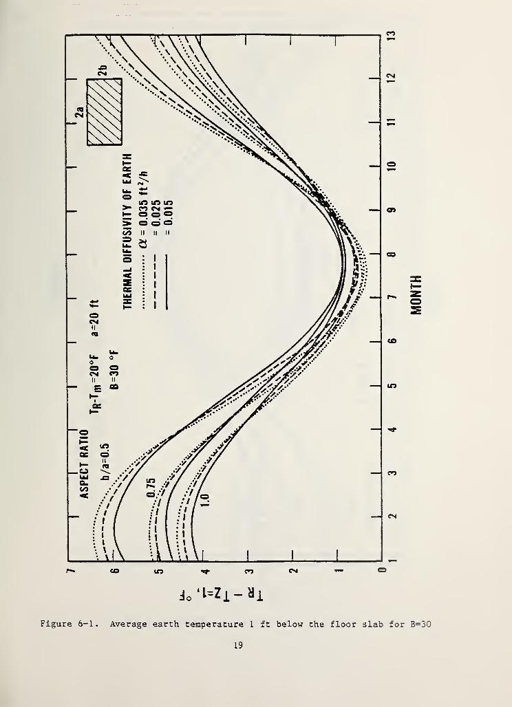
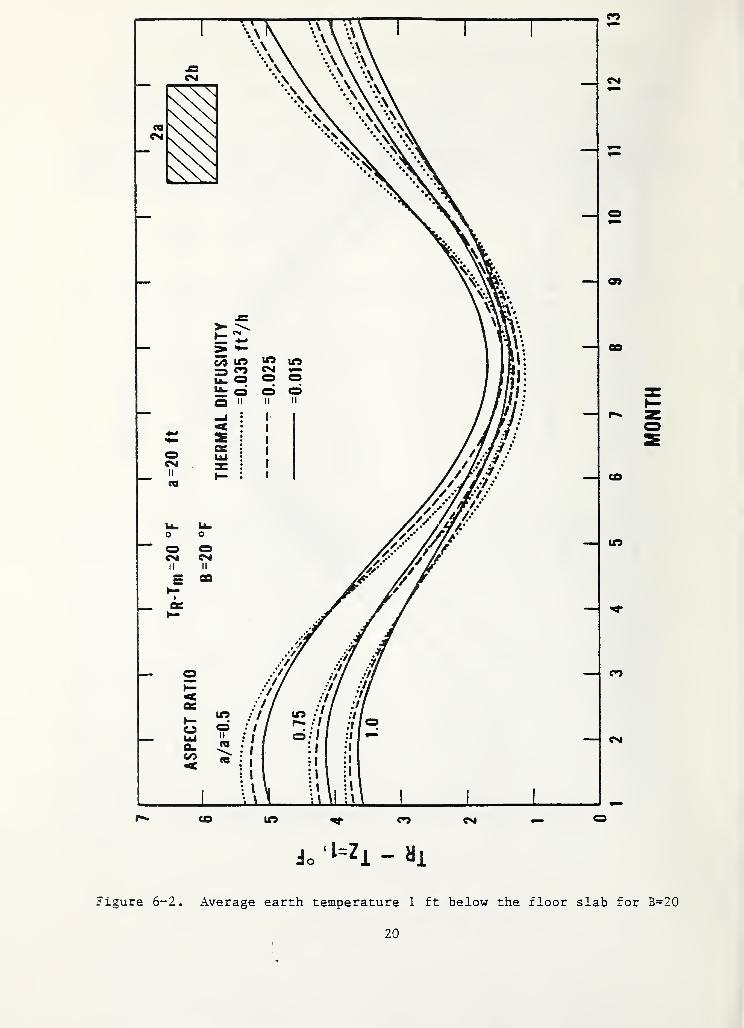
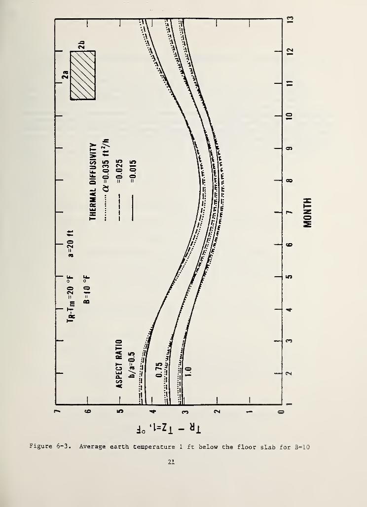
Figure 6-1, 2, 3 shows the sample results of such calculations for TR - Tm = 20°F,and 3 = 30, 20 and 10°F, respectively, for z = 1 ft. They represents the areaaverage earth temperature 1 ft below the floor slab of 20 ft x 40 ft, 30 ft x40 ft and 40 ft x 40 ft. These figures show a surprisingly small effect of
soil thermal diffusivity upon the sub-slab temperature for all seasons, andshow a larger effect of floor aspect ratio during the winter. The use of thesefigures for the estimation of floor heat loss, however, requires the knowledgeof annual average soil temperature Tm (which is very close to the deep under-ground or the well water temperature), and annual maximum and minimum monthlynormal outdoor temperatures, all of which are readily available from the U.S.Weather Record Center [10]. For example, according to [9], the annual averagetemperature, annual maximum and minimum for the monthly normal (30-year average)data for Washington, D.C. are 56.8°F, 77.8°F and 36.5°F, respectively. From
this, one can arrive at Tm = 56.5°F, and B = (77 .8—36 .5)/ 2 = 20.65°F or say 20°F.Using figure 6-2, one can then estimate the seasonal floor slab heat loss for
the slab having temperature of 56.5 + 20 = 76.5°F, provided that the thermalproperties of the slab are very similar to those of the soil beneath the floor.
If one assumes that the soil has the thermal diffusivity of 0.025 ft 2/h, ther-
mal conductivity 0.5 Btu/h*ft*F, and the floor-slab is 30 ft x 40 ft (aspectratio 0.75), the following floor heat loss calculation can be made fromfigure 6-2.
18
P-* CO CO <N
Figure 6-1. Average earth temperature 1 ft below the floor slab for B=30
19
MONTH
CD LT5 Tf> CO CN
do‘ l=Zi - »1
Figure 6-2. Average earth temperature 1 ft below the floor slab for B=20
20
MONTH
Jo ‘l=Zl -
co
CM
03
CO
CO
ITS
cn
CNt
Figure 6-3. Average earth temperature i ft below the floor slab for B=10
21
MONTH
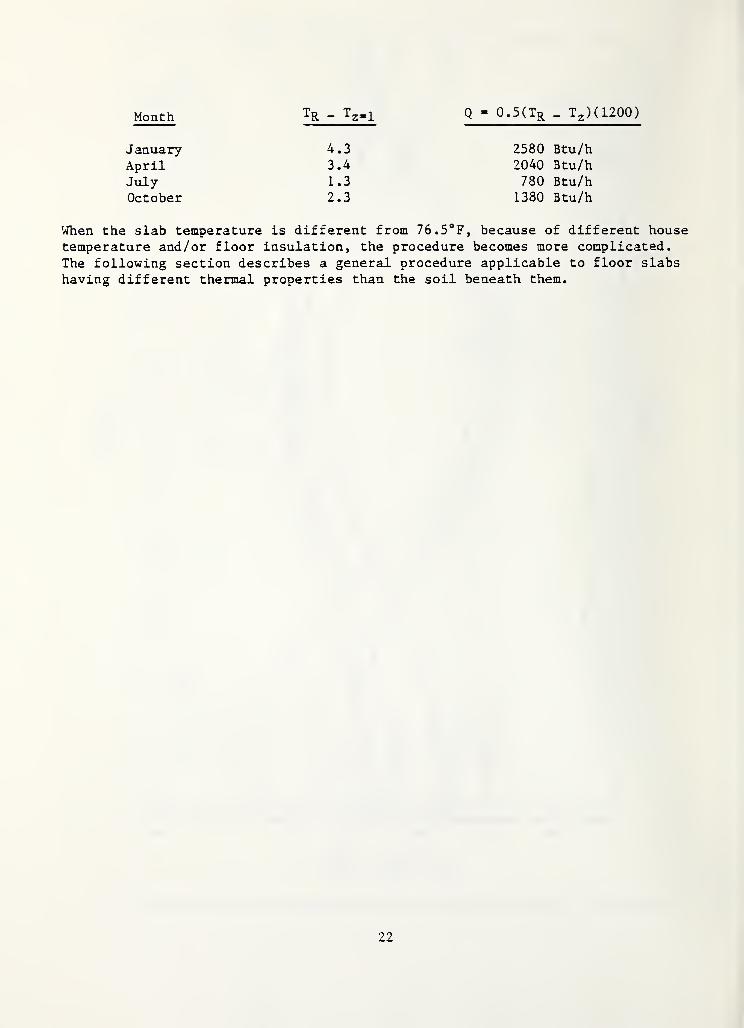
Month Tr - t2=1 Q = 0.5(Tr _ T z ) (1200
)
January 4.3 2580 Btu/hApril 3.4 2040 Btu/hJuly 1.3 780 Btu/hOctober 2.3 1380 Btu/h
When the slab temperature is different from 76.5°F, because of different housetemperature and/or floor insulation, the procedure becomes more complicated.
The following section describes a general procedure applicable to floor slabshaving different thermal properties than the soil beneath them.
22
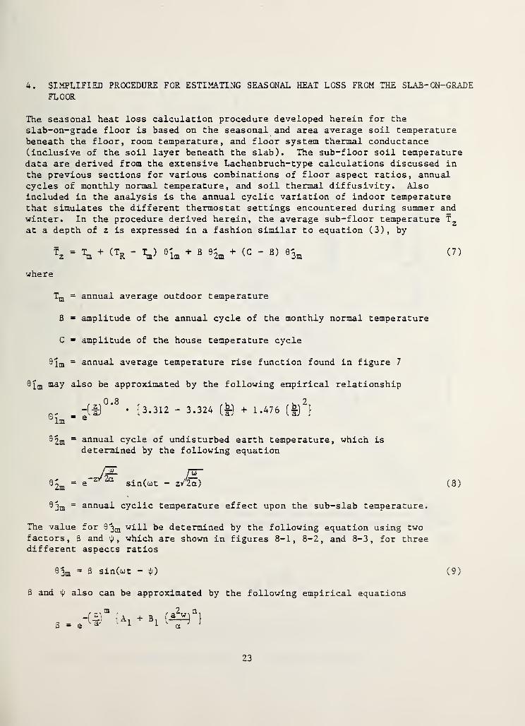
4. SIMPLIFIED PROCEDURE FOR ESTIMATING SEASONAL HEAT LOSS FROM THE SLAB-ON-GRADEFLOOR
The seasonal heat loss calculation procedure developed herein for the
slab-on-grade floor is based on the seasonal and area average soil temperaturebeneath the floor, room temperature, and floor system thermal conductance(inclusive of the soil layer beneath the slab). The sub-floor soil temperaturedata are derived from the extensive Lachenbruch-type calculations discussed in
the previous sections for various combinations of floor aspect ratios, annualcycles of monthly normal temperature, and soil thermal diffusivity. Alsoincluded in the analysis is the annual cyclic variation of indoor temperaturethat simulates the different thermostat settings encountered during summer and
winter. In the procedure derived herein, the average sub-floor temperature Tz
at a depth of z is expressed in a fashion similar to equation (3), by
Tm = annual average outdoor temperature
B = amplitude of the annual cycle of the monthly normal temperature
C = amplitude of the house temperature cycle
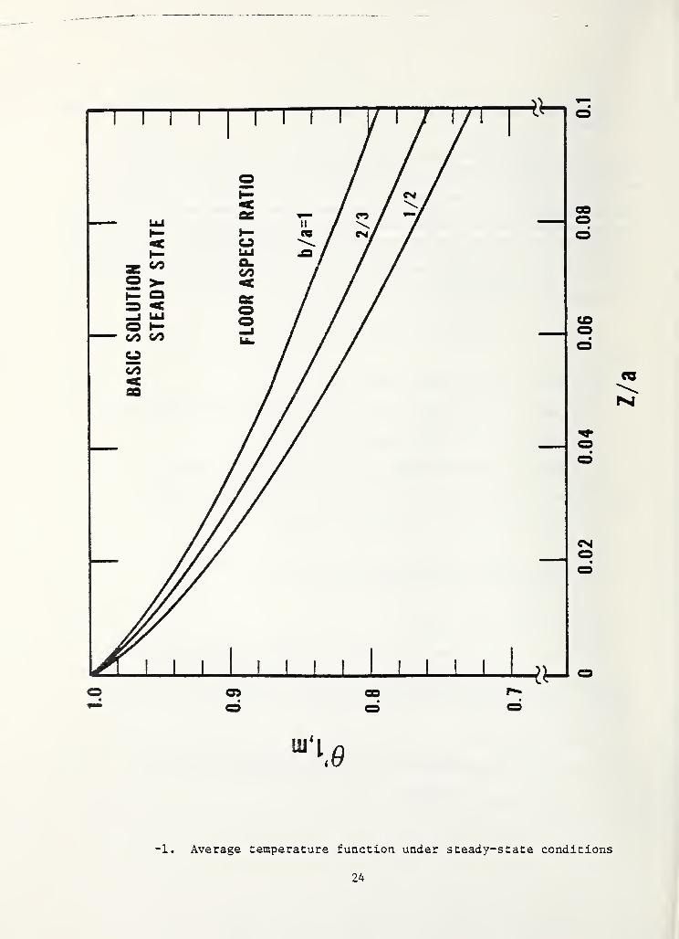
®lm= annual average temperature rise function found in figure 7
dfm may also be approximated by the following empirical relationship
93m = annual cyclic temperature effect upon the sub-slab temperature.
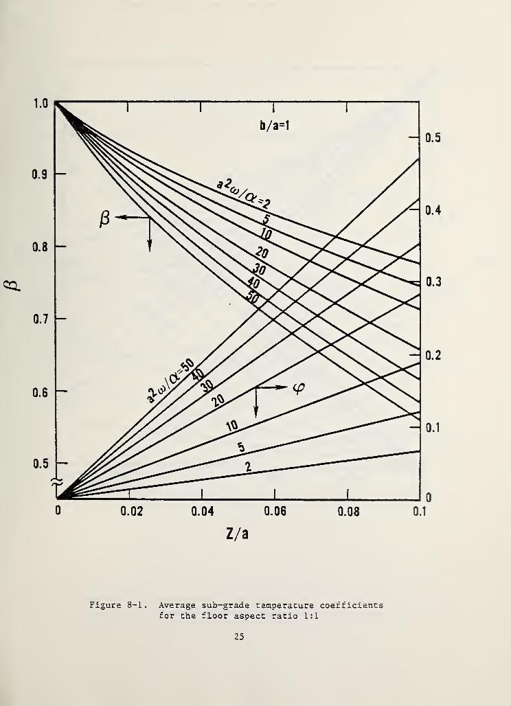
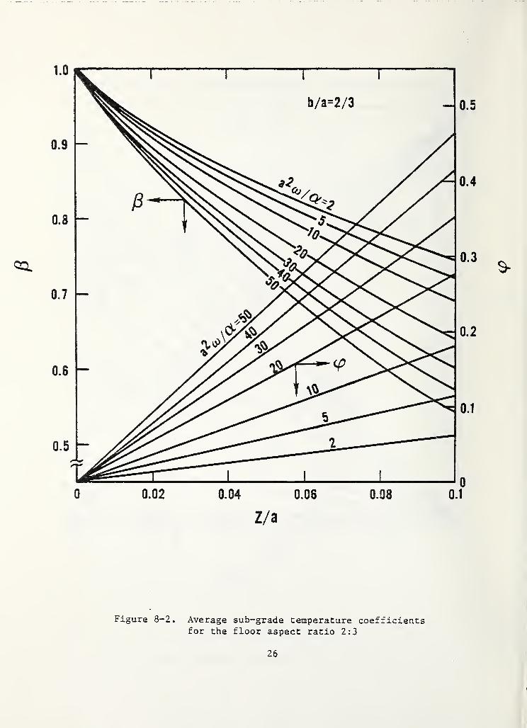
The value for 63^ will be determined by the following equation using twofactors, 8 and 'p
,which are shown in figures 8-1, 8-2, and 8-3, for three
different aspects ratios
L - \ + (TR ' V 9lm
+ B «2m+ < c ' B > 9 3m (7)
where
® 2m= annual cycle of undisturbed earth temperature, which is
determined by the following equation
( 8 )
9 3m= 3 sin((Dt - ip) ( 9 )
8 and 'p also can be approximated by the following empirical equations
23
BASIC
SOLUTION
STEADY
STATE
-1. Average temperature function under steady-state conditions
24
0.02
0.04
0.06
0.08
Z/a
Figure 8-1. Average sub-grade temperature coefficientsfor the floor aspect ratio 1:1
25
3-
Figure 8-2. Average sub-grade temperature coefficientsfor the floor aspect ratio 2:3
26

$-
Figure 8-3. Average sub-grade temperature coefficientsfor the floor aspect ratio 1:2
27

where A, = 2.919 - 3.029 (-^) + 1.362 (^-)"
a a
B, = 0.1957 + 0.0936 (-^) + 0.0144 (-^)2
a a
n = 0.6773 + 0.0141 (b.) - 0.0426 (&)2
a a
m =(a^w) 0,035
(0.756 + 0.046 (Vj j
a ^ a'
9 Ei — F i' a
* - {c + d^A)} (ibqx A a a
where values of, Dj,
a^wa
and may be f ound in table as a function of
Cl Dl El El
1.8 <a2w
< 7a
0.236 0.168 0.800 0.111
X,7 <
a w< 16
a
0.278 0.207 0.713 0.119
16 < <45
a
0.372 0.170 0.623 0.067
The floor heat loss is then calculated by knowing the overall thermalconductance Uq of the soil layer of thickness l such that
Q - V TR ' VA (10)
and U_ = Jl .(ID
G i
Insulated slab-floor
While the preceding analysis assumes that the floor slab has the same thermalproperties as those of the soils below (which is approximately correct for
uninsulated concrete floor over relatively wet soil), many floor systems includethermal insulation with their thermal property data being considerably differentfrom those of the sub-soil. When dealing with an insulated floor, one mustaccount for an appreciable temperature drop across it. Thus the values of Tg_
28
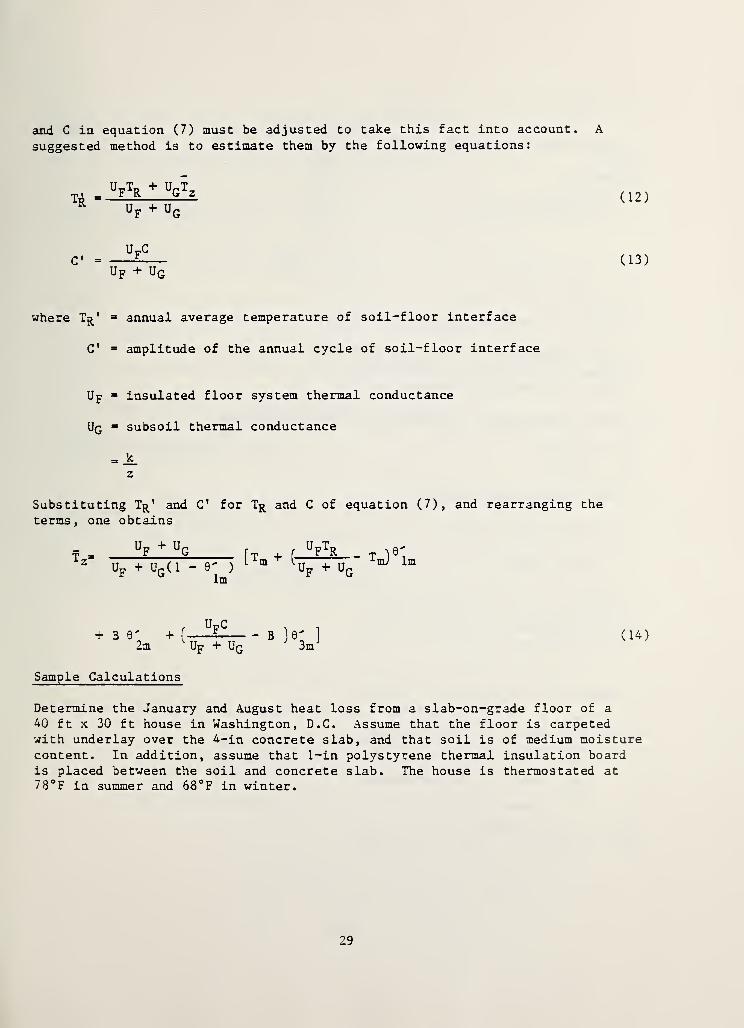
and C in equation (7) must be adjusted to take this fact into account. A
suggested method is to estimate them by the following equations:
TrUFTR + U
GTz
uF + uG
UFC
Up + Ug
( 12 )
(13)
where T^'
C'
annual average temperature of soil-floor interface
amplitude of the annual cycle of soil-floor interface
Up = insulated floor system thermal conductance
Uq = subsoil thermal conductance
= _k_
z
Substituting TR* and C 1 for Tr and C of equation (7), and rearranging the
terms, one obtains
TUp + UG
Up + UG (1 - 9'
)
lm
[Tm + t
UFTR
Up + uG^m] lm
+ B 92m
+ (
uFc
Up + UGB 6'
3m'
Sample Calculations
(14)
Determine the January and August heat loss from a slab-on-grade floor of a
40 ft x 30 ft house in Washington, D.C. Assume that the floor is carpetedwith underlay over the 4-in concrete slab, and that soil is of medium moisturecontent. In addition, assume that 1-in polystyrene thermal insulation boardis placed between the soil and concrete slab. The house is thermostated at78°F in summer and 68°F in winter.
29
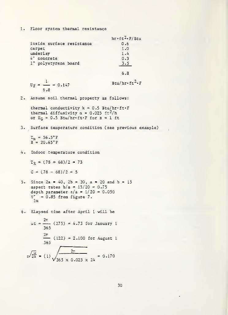
1.
Floor system thermal resistance
hr«f t^.F/Btuinside surface resistancecarpetunderlay4" concrete1” polystyrene board
0.61.0
1.4
0.33.5
6.8
1
Up - =0.1476.8
Btu/hr» f t“» F
2. Assume soil thermal property as follows:
thermal conductivity k = 0.5 Btu/hr*ft«Fthermal diffusivity a = 0.025 ft^/hor UG = 0.5 Btu/hr*ft»F for z = 1 ft
3. Surface temperature condition (see previous example)
Tm = 56 .5° F
B = 20 .65° F
4. Indoor temperature condition
T r = (78 + 68 ) / 2 = 73
C = (78 - 68)/ 2 = 5
5. Since 2a = 40 , 2b = 30 , a = 20 and b = 15
aspect rates b/a = 15/20 = 0.75depth parameter z/a = 1/20 = 0.0503' = 0.85 from figure 7.lm
6. Elapsed time after April 1 will be
tut = (275) = 4.73 for January 1
365
2r(122) = 2.100 for August 1
365
365 x 0.025 x 240.170
30
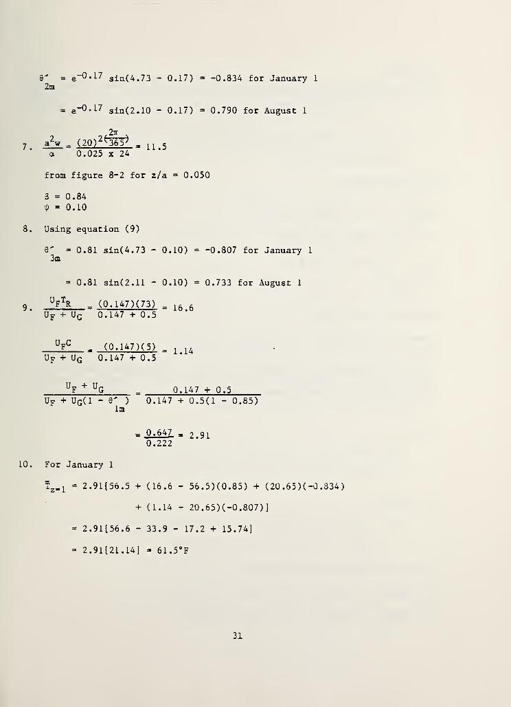
Q' = e 0.17 sin(4.73 - 0.17) = -0.834 for January 1
2m
= e”0.17 gin(2.10 - 0.17) 3 0.790 for August 1
7 a2v . (20) 2e365^ _ „ c
* a 0.025 x 24
from figure 8-2 for z/a = 0.050
8 = 0.84
if;= 0.10
8. Using equation (9)
0" = 0.81 sin(4.73 - 0.10) = -0.807 for January 1
3m
= 0.81 sin(2.11 - 0.10) = 0.733 for August 1
oUF
TR , (0.147 ) (73) , ^ &
Up + U G 0.147 + 0.5
UFC = (0.147H5) = L 14Up + UG 0.147 + 0.5
UF+ U
G = 0.147 + 0.5Up + UG (1 - 9
') 0.147 + 0.5(1 - 0.85)
lm
= 0-647. = 2.910.222
10. For January 1
Tz=1 = 2.91 [56.5 + (16.6 - 56.5)(0.85) + ( 20 .65 ) (-0 .834)
+ (1.14 - 20 .65) ( -0 .807 )
]
= 2.91 [56.6 - 33.9 - 17.2 + 15.74]
=* 2.91 [21.14] = 61.5°F
31
For August 1
Tz=1 = 2.91 [56.5 + (16.6 - 56.5) (0.85) + (20.65)(0.79)
+ (1.14 - 20.65X0.733)]
= 2.91 [56.5 - 33.9 + 16.31 - 14.30]
= (2.91X24.61) = 71.6
11. House temperature
January 1 : 73 + 5 sin(4.73) = 68°FAugust 1 : 73+5 sin(2.10) = 79°F
12. Floor/soil thermal conductance
I = I_ + _L_ = 6.8 + 2 = 8.8u U F UG
U = 0.1136
13. Floor heat loss is then
January : (0.11367) (68 - 61 . 5 ) ( 1200 ) =* 886 Btu/hAugust : (0.1136X77 - 71.8)( 1200) = 736 Btu/h
If similar calculations are performed for the non-insulated slab floorwhereby the slab thermal properties are nearly equal to those of the soilbelow, equation (7) may be used directly to find the sub-soil temperature1 ft below the floor surface as follows.
January 1:
Tz=1 : 56.5 + (73 - 56.5X0.85) + (20.65X-0.834) + (5 - 20.65)(-0.807)
= 56.5 + 14.03 - 17.22 + 12.63 = 65.9
For August 1:
T z=1 : 56.5 + (73 - 56.5X0.85) + (20 .65) (0.79) + (5 - 20 .65) (0.733)
= 56.5 + 14.03 + 16.30 - 11.47 = 75.4
The floor heat loss would then be
for January : (0.5)(68 - 65.9)(1200) = 1260 Btu/h
for August : (0.5)(77 - 75.4)(1200) = 960 Btu/h
32

These calculations show that the subfloor temperature is lower when the floorsare insulated than otherwise. Comparison of the uninsulated floor heat loss
with that determined by the ASHRAE Handbook equation could yield
q = (0.81 )( 140)(68 - 36.5) = 3572 Btu/h
when the winter outdoor temperature is assumed 36. 5° F.
33
5. SUMMARY AND DISCUSSION
Monthly depth profiles of the earth temperature beneath the floor slab have beendetermined by using the Lachenbruch method. The results were used to develop a
simplified procedure for calculating the area average temperature beneath the
slab floor area. The area-averaged earth temperature can in turn be used to
approximate the monthly floor heat loss. In addition, the area-averaged sub-floor earth temperature determined by this method should be good referencedata for the response factor-type evaluation of hourly floor heat transfer.
Caution must be exercised, however, for the use of average sub-floor soiltemperatures in the calculation of the floor heat loss, because the methodignores several important facts.
1. The floor foundation effect: The floor slab is usually mounted on a
concrete foundation of complex shape around its edge. These concretefoundations could cause additional complexity in the temperature fieldaround the floor slab because of differences in thermal conductivityfrom the surrounding soil.
2. The edge insulation: Some slab-on-grade floors employ insulationaround their edges, which would yield different temperature fieldsthan predicted by the procedure developed in this paper.
3. Building wall thickness effect: The analysis employed in the proposedprocedure assumes that the slab temperature is uniform from one end of
the floor to another, and assumes an abrupt temperature drop at the
edge from the indoor condition to outdoor condition. In reality, the
slab temperature would undergo a gradual change near the edge, and the
transition temperature profile from the indoor condition to the outdoorcondition depends heavily upon the thickness and thermal characteris-tics of the wall over the slab edge. If the wall is thicker and betterinsulated, the temperature transition would be steeper than the thinnerand poorly insulated wall.
The Lachenbruch procedure employed in this paper could simulate the
nonuniform slab temperature as long as its profile is known. Muncey/Spencer [6] relation can indeed take into account the building wallproblem by assuming prescribed slab-to-outdoor temperature distributionfunctions
.
One of the dubious aspects of this area-averaged sub-floor earth temperatureconcept is that the depth for which the area averaging is to be performed is not
well defined. If the depth is too great, the edge heat loss effect will not be
adequately reflected. On the other hand, if the depth is too small, the edge
effect will be overated with the reason discussed above, in reference to the
wall thickness effect. In fact, a preliminary result of the heat flux measure-ment on the NBS test house (in Gaithersburg, MD) during January of 1981, indi-
cated that the edge effect on a 20 ft x 20 ft slab-on-grade house is not as
severe as that calculated by equation (4). It appears that the use of area-averaged earth temperatures 1 ft below the slab provides a good base for the
feasonal slab-heat-loss calculation, although further and detailed validation.ffort is needed.
34
6
.
REFERENCES
1. Chapter 24, "Heating Load," Handbook of Fundamentals ,ASHRAE, page 24.4,
1977.
2. R. S. Dill, W. C. Robinson, and H. E. Robinson, "Measurements of Heat
Losses from Slab Floors," NBS Building Material and Structures Report
BMS 103 , March 1943.
3. H. D. Bareither, A. N. Fleming, and B. E. Alberty, "Temperature and Heat
Loss Characteristics of Concrete Floors Laid on the Ground,” Universityof Illinois Small Homes Council Technical Report ,
PB 93920, 1948.
4. A. H. Lachenbruch, "Three Dimensional Heat Conduction in Permafrost BeneathHeated Buildings," Geological Survey Bulletin 1052-B
,U.S. Government
Printing Office, Washington, D.C., 1957.
5. B. Adamson, "Soil Temperature Under Houses Without Basements,"Byggforskningen Handlinger, Nr 46 Transactions, 1964.
6. R. W. R. Muncey and J. W. Spencer, "Heat Flow into the Ground Under a
House," Energy Conservation in Heating, Cooling, and Ventilating Buildings,
Hemisphere Publishing Corporation, Washington, D.C., Vol. 2, pp. 649-660,1978.
7. H. Akasaka, "Calculation Methods of the Heat Loss Through a Floor andBasement Walls," Transactions of the Society of Heating, Air-Conditioning ,
and Sanitary Engineers of Japan , No. 7, pp. 21-35, June 1978.
8. T. Kusuda, "Review of Current Calculation Procedures for Building EnergyAnalysis," National Bureau of Standards NBSIR 80-2068, July 1980.
9. T. Kusuda, "Thermal Response Factors for Multi-Layer Structures of VariousHeat Conduction Systems" ASHRAE Transactions
, pp. 250-269, Part I, 1969.
10. ,"Monthly Normal Temperatures, Precipitations and Degree
Days," U.S. Weather Bureau, U.S. Department of Commerce, Washington, D.C.
,
1956.
35

APPENDIX A
Muncey/ Spencer Solution
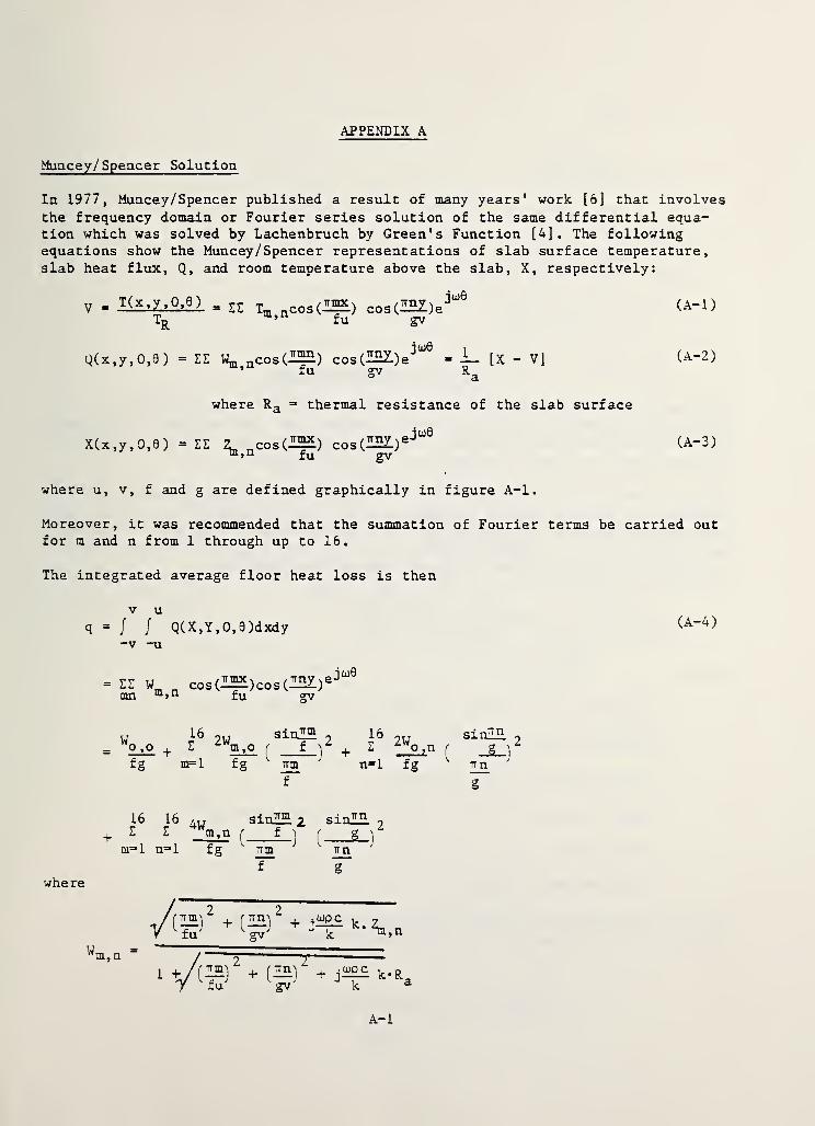
In 1977, Muncey/ Spencer published a result of many years’ work [6] that involves
the frequency domain or Fourier series solution of the same differential equa-tion which was solved by Lachenbruch by Green's Function [4]. The followingequations show the Muncey/ Spencer representations of slab surface temperature,slab heat flux, Q, and room temperature above the slab, X, respectively:
V = T(x ’y>°' 6) = ££ Tm acos(I22.) cos(IHI)e3 “6 <A-D
Tr * fu gv
Q(x,y,0,9) = ZZ ncos (-H52-) cos(^E2-)e^ = — [X - V] (A-2)’ fu gv R
a
where Ra = thermal resistance of the slab surface
XU,y,0,9) = ££ 2 cos(I2*) cos(™l) ej“e
(A-3)fu 2V
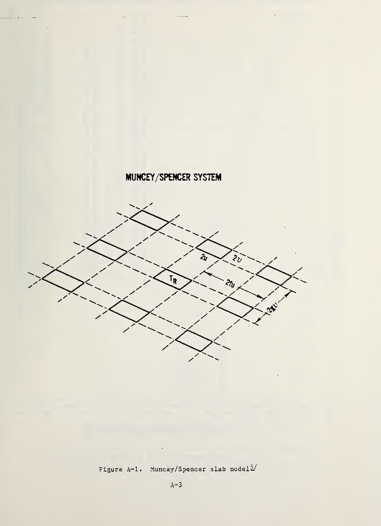
where u, v, f and g are defined graphically in figure A-l.
Moreover, it was recommended that the summation of Fourier terms be carried outfor m and n from 1 through up to 16.
The integrated average floor heat loss is then
v u
q * / / Q(X,Y,0,9)dxdy-v -u
ZZ Wmn n
cos(IHi)cos(IHZ)£u gv
ej uQ
Wo,o +r ^ 2WI
zwm,osinjrm
ff
1
0 16
+ Z
fg m=l fg urn
T~n=l
16 16Z Z
r
sin Ttm2
fi r
c-j n 1Tn
g_l2
2W sin:o ,n
ini
g
fg Tm
gwhe re
IB)
2+ ( IB)
2+ ji££
fu gv kW.
1 V(^)Z+ + k.R
£gv
(A-4)
A-l
z0,0 fg
Zm,o
JL sinCLSL)umg f
Zo , n
JL sinOH)Tinf g
a = k_ orcp k a
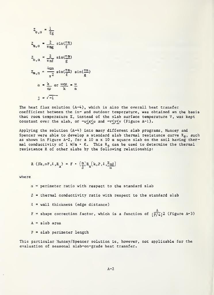
The heat flux solution (A-4), which is also the overall heat transfercoefficient between the in- and outdoor temperature, was obtained on the basisthat room temperature X, instead of the slab surface temperature V, was keptconstant over the slab, or -u<x<u and -vCy<v (Figure A-l).
Applying the solution (A-4) into many different slab programs, Muncey and
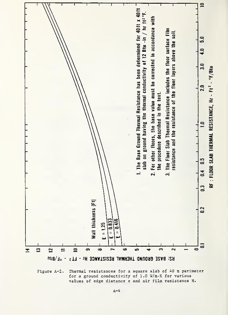
Spencer were able to develop a standard slab thermal resistance curve Rs ,such
as shown in Figure A-2 , for a 10 m x 10 m square slab on the soil having ther-mal conductivity of 1 W/m • K. This Rs can be used to determine the thermalresistance R of other slabs by the following relationship:
a = perimeter ratio with respect to the standard slab
6 - thermal conductivity ratio with respect to the standard slab
l = wall thickness (edge distance)
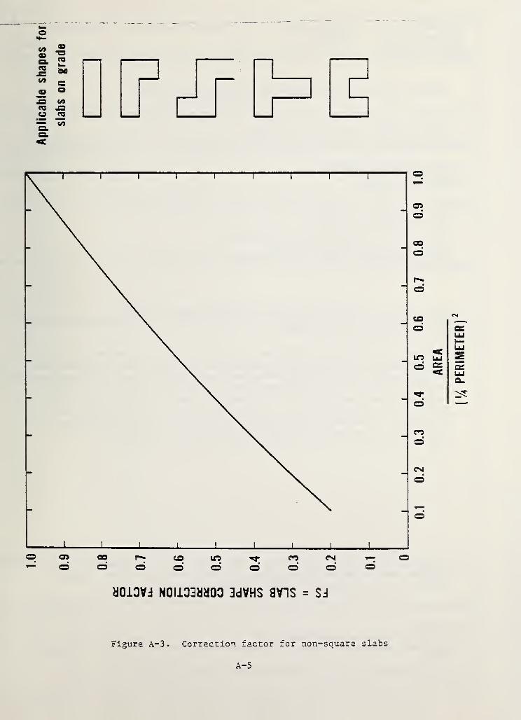
AF = shape correction factor, which is a function of
[ p/ 4 ] 2 (Figure A-3
A = slab area
P = slab perimeter length
This particular Muncey/Spencer solution is, however, not applicable for the
evaluation of seasonal slab-on-grade heat transfer.
where
A-2
MUNCEY/SPENCER SYSTEM
Figure A-l. Muncey/Spencer slab model!/
pin
co
CM
ino
co
CM
m/ic z id • J H 33N»lSIS3a 1VNH3H1 QNnOUS 3SV9 -SS
Figure A- 2 . Thermal resistances for a square slab of 40 m perimeterfor a ground conductivity of 1.0 W/m-K for variousvalues of edge distance e and air film resistance H.
A-4
RF
:
FLOOR
SLAB
THERMAL
RESISTANCE,
Hr
-
Ft2
-
°F/Btu
</>
05o
CO
in
cn
CM
CM
aoiovj Hoii33aaoa aavns a\ns = sj
Figure A-3 . Correction factor for non-square slabs
A-
5
AREA
{%
PERIMETER)

NBS-U4A ( REV. 2-60
U.S. DEPT. OF COMM.
BIBLIOGRAPHIC DATASHEET (See instructions)
1. PUBLICATION ORREPORT NO.
NBSIR 81-2420
2. Performing Organ. Report No. 3. Publication Date
Feb' lary 19824.
TITLE AND SUBTITLE
SEASONAL HEAT LOSS CALCULATION FOR SLAB-ON-GRADE FLOORS
5.
AUTHOR(S)
Tamami Kusuda; M. Mizuno; J.W. Bean
6.
PERFORMING ORGANIZATION (If joint or other than NBS. see in struction s)
NATIONAL BUREAU OF STANDARDSDEPARTMENT OF COMMERCEWASHINGTON, D.C. 20234
7. Contract/Grant No.
S. Type of Report & Period Covered
9.
SPONSORING ORGANIZATION NAME AND COMPLETE ADDRESS (Street. City. State. ZIP)
U.S. Department of EnergyOffice of Solar Application for BuildingsConservation and Renewable Energy1000 Independence Avenue, SW - Washington, DC 20585
10.
SUPPLEMENTARY NOTES
j jDocument describes a computer program; SF-185, FIPS Software Summary, is attached.
11.
ABSTRACT (A 200-word or less factual summary of most significant information. If document includes a si gnificantbi bl iography or literature survey, mention it here)
In order to facilitate an efficient slab-on-grade heat transfer calculation ona comprehensive energy analysis program such as DoE-2, BLAST and NBSLD heattransfer calculations for slab-on-grade floors are reviewed. The computationalprocedure based on the Lachenbruch method is studied in depth to generatemonthly average temperatures at a given depth below the floor slab. The datagenerated by the Lachenbruch method are then used to develop a simplifiedprocedure for determining the monthly average earth temperatures below thefloor slab. These monthly average temperature data can be used for thehourly response factor analysis of floor-slab heat transfer.
12. KEY WORDS (Six to twelve entries; alphabetical order; capitalize only proper names; and separate key words by semicolons)
Building heat transfer; DoE-2 Energy Analysis computer program; monthlyaverage earth temperature; thermal response factors.
13. AVAILABILITY 14. NO. OFPRINTED PAGES
| y |
Unlimited
49| j
For Official Distribution. Do Not Release to NTIS
| |Order From Superintendent of Documents, U.S. Government Printing Office, Washington, D.C.
15. Price20402.
jXI Order From National Technical Information Service (NTIS), Springfield, VA. 22161 $7.50
J
’JSCOMM-OC 3043-PS


![Slab on Grade en[1]](https://img.pdfslide.net/doc/110x75/577d24b91a28ab4e1e9d371c/slab-on-grade-en1.jpg)