Seasonal predictability of daily rainfall statistics over ...awr/TP/Indonesia/Papers/RobertsonMoronSwarinoto_IJC08.pdf · Seasonal predictability of daily rainfall statistics over

INTERNATIONAL JOURNAL OF CLIMATOLOGYInt. J. Climatol. (2008)Published online in Wiley InterScience(www.interscience.wiley.com) DOI: 10.1002/joc.1816

Seasonal predictability of daily rainfall statistics overIndramayu district, Indonesia

Andrew W. Robertson,a* Vincent Morona,b and Yunus Swarinotoc

a International Research Institute for Climate and Society (IRI) Columbia University, New York, USAb CEREGE, the University of Aix-Marseille, and the Institut Universitaire de France, France

c Bureau of Meteorology and Geophysics, Indonesia

ABSTRACT: The seasonal predictability of rainfall over a small rice-growing district of Java, Indonesia is investigated interms of its daily characteristics during the September–December monsoon-onset season. The seasonal statistics consideredinclude rainfall frequency, mean daily intensity, median length of dry spells, as well as the onset date of the rainy season.General circulation model retrospective seasonal forecasts initialized on August 1 are downscaled to a set of 17 stationlocations using a nonhomogeneous hidden Markov model. Large ensembles of stochastic daily rainfall sequences aregenerated at each station, from which the seasonal statistics are calculated and compared against observations usingdeterministic and probabilistic skill metrics. The retrospective forecasts are shown to exhibit moderate skill in terms ofrainfall frequency, seasonal rainfall total, and especially monsoon onset date. Some skill is also found for median dry-spelllength, while mean wet-day persistence and daily rainfall intensity are not found to be predictable. Copyright 2008Royal Meteorological Society

KEY WORDS seasonal predictability; Indonesia; hidden Markov model

Received 3 July 2008; Revised 22 October 2008; Accepted 26 October 2008

1. Introduction

Seasonal climate forecasts are typically issued in termsof three-month averages of rainfall or temperature, as acompromise between maximizing the ratio of predictableclimate signal to unpredictable weather noise, while stillcapturing seasonal evolution (e.g. Goddard et al., 2001).However, such seasonally averaged forecasts are often oflimited use to decision makers, where risk managementin agriculture, for example, may require information onaspects such as the onset of the rainy season, or theprobability of rainfall occurrence, long dry spells, orrainfall extremes within the growing season. In addition,the skillful spatial scale of current general circulationmodal (GCM) seasonal predictions is of the order ofseveral hundred kilometers (Gong et al., 2003), againmuch larger than may be required for effective climaterisk management at the scale of a small administrativedistrict. Downscaling is required, within the physicalconstraints of the regional climate system, and thelimitations of available downscaling methodologies.

Recent work suggests that in the tropics, rainfall fre-quency at the station scale is more seasonally predictablethan the seasonal total of rainfall; this is primarily dueto the relatively higher spatial coherence of interannual

* Correspondence to: Andrew W. Robertson, International ResearchInstitute for Climate and Society (IRI), Columbia University LamontCampus, 61 Route 9W, Palisades, NY 10960, USA.E-mail: [email protected]

anomalies of rainfall frequency compared to those ofmean daily rainfall intensity (Moron et al., 2006, 2007).

Probabilistic models of “weather within climate” withdaily resolution based on stochastic weather genera-tors, hidden Markov models, and K-nearest neighborsapproaches have been used to express GCM-based sea-sonal forecasts in terms of ensembles of stochastic localdaily weather sequences that can then, in principle, beused to drive models of crop growth and yield (Hansenand Ines, 2005; Ines and Hansen, 2006; Robertson et al.,2007; Moron et al., 2008d). The nonhomogeneous hiddenMarkov model (NHMM) has proved to be a promis-ing method for constructing multistation weather genera-tors (Hughes and Guttorp, 1994). Over northeast Brazil,Robertson et al. (2004) found that interannual variabilityin the frequency-of-occurrence of 10-day dry spells couldbe simulated reasonably, using an NHMM with GCMseasonal-mean large-scale precipitation as a predictor.Similar downscaling results were obtained over Queens-land, Australia (Robertson et al., 2006). The NHMM hasbeen applied to two other locations in Australia in down-scaling studies (Charles et al., 2003, 2004).

In this paper, retrospective GCM seasonal precipitationforecasts are downscaled to a set of rainfall stations overIndramayu, a small (2140 km2) flat coastal district ofWest Java, using an NHMM and their skill assessedunder cross-validation. We focus on a set of weatherstatistics of potential relevance to agriculture, namelydaily rainfall frequency, mean daily intensity on wetdays, mean dry-spell lengths, wet-day persistence, and the

Copyright 2008 Royal Meteorological Society

A. W. ROBERTSON ET AL.

monsoon onset date, in addition to the seasonal rainfalltotal. Deterministic and probabilistic measures of skill arequantified.

Rainfall over Indonesia is governed by the austral-Asian (northwest) monsoon, whose onset progresses fromnorthwest-to-southeast during the austral spring (Aldrianand Susanto, 2003). Many studies have shown that theEl Nino – Southern Oscillation (ENSO) exerts itsstrongest influence on Indonesian rainfall during theSeptember–December monsoon onset season (e.g.,Hamada et al., 2002; Juneng and Tangang, 2005). Theimpact of ENSO then diminishes during the core ofthe rainy season in December–February (Haylock andMcBride, 2001; Aldrian et al., 2005, 2007; Gianniniet al., 2007), suggesting that the timing of monsoon onsetmay be potentially predictable. Moron et al. (2008a,b)have recently argued that much of the seasonal pre-dictability in the September–December total rainfall isassociated with changes in monsoon onset date.

Indramayu, situated on the north coast of West Java,is an important rice-growing district contributing aboutone-quarter of Java’s rice production. Farmers experiencedroughts and floods that cause significant losses in riceproduction. The date of onset of the rainy season isof particular importance, determining the suitable timefor planting crops, while delayed onset during El Ninoyears (Hamada et al., 2002; Naylor et al., 2002; Boerand Wahab, 2007) can lead to crop failure. Earlier onsetsoccur in La Nina years, but these are generally lesspronounced than the delays during El Nino (Moron et al.,2008b); these may, however, be potentially beneficial tofarmers by extending the length of the growing season.“False rains”, in which isolated rainfall events occuraround the expected onset date also present problems forfarmers.

This paper is motivated by the needs of the IndonesianBureau of Meteorology and Geophysics (BMG), whichhas been working with the agricultural office to developclimate forecasts that are specific to agriculture overIndramayu. The September–December season is selectedfor its importance to agriculture as well as its relatively

high seasonal predictability of rainfall. The paper isorganized as follows. Section 2 describes the rainfalldata and GCM simulations, Section 3 describes thehidden Markov model and statistical methods. The resultsare presented in Section 4, with conclusions given inSection 5.

2. Data

2.1. Observed rainfall data

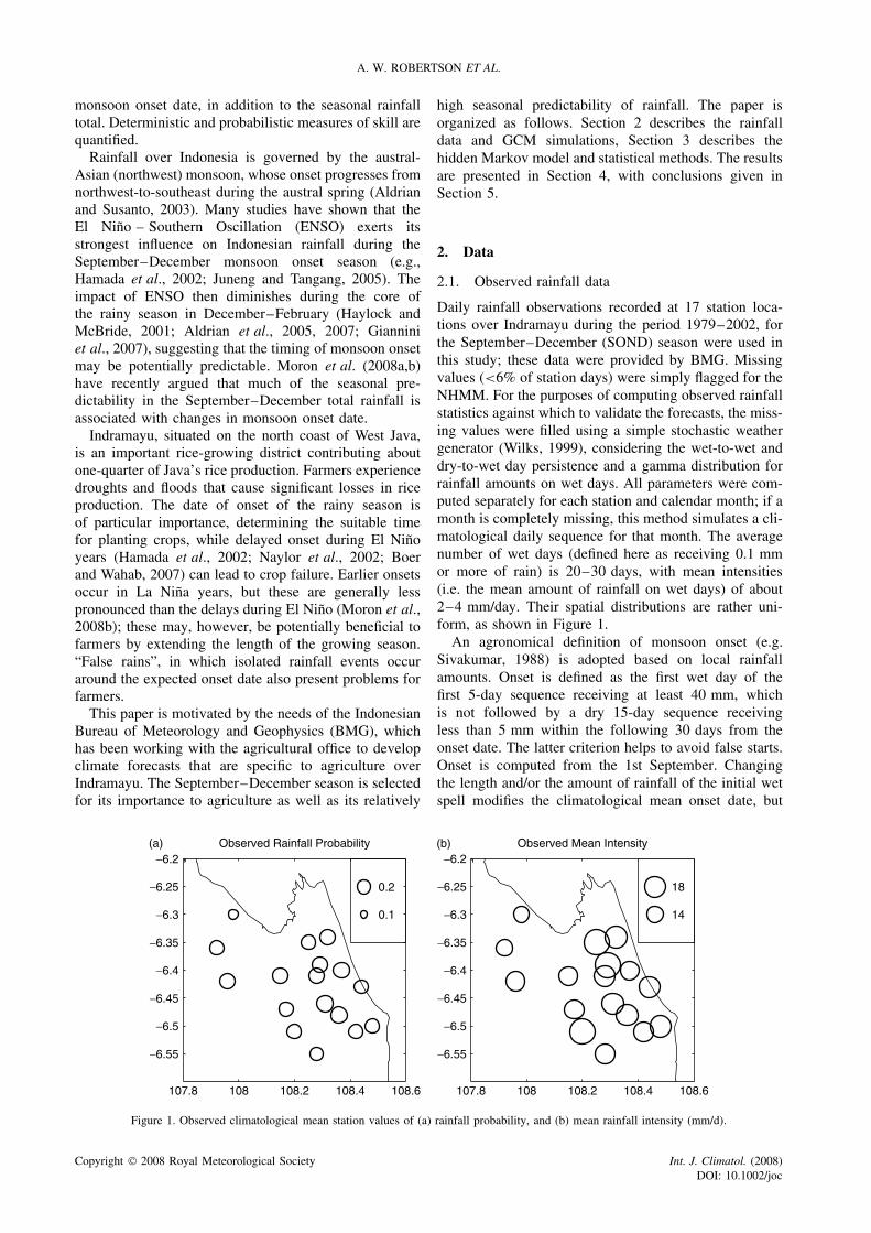
Daily rainfall observations recorded at 17 station loca-tions over Indramayu during the period 1979–2002, forthe September–December (SOND) season were used inthis study; these data were provided by BMG. Missingvalues (<6% of station days) were simply flagged for theNHMM. For the purposes of computing observed rainfallstatistics against which to validate the forecasts, the miss-ing values were filled using a simple stochastic weathergenerator (Wilks, 1999), considering the wet-to-wet anddry-to-wet day persistence and a gamma distribution forrainfall amounts on wet days. All parameters were com-puted separately for each station and calendar month; if amonth is completely missing, this method simulates a cli-matological daily sequence for that month. The averagenumber of wet days (defined here as receiving 0.1 mmor more of rain) is 20–30 days, with mean intensities(i.e. the mean amount of rainfall on wet days) of about2–4 mm/day. Their spatial distributions are rather uni-form, as shown in Figure 1.

An agronomical definition of monsoon onset (e.g.Sivakumar, 1988) is adopted based on local rainfallamounts. Onset is defined as the first wet day of thefirst 5-day sequence receiving at least 40 mm, whichis not followed by a dry 15-day sequence receivingless than 5 mm within the following 30 days from theonset date. The latter criterion helps to avoid false starts.Onset is computed from the 1st September. Changingthe length and/or the amount of rainfall of the initial wetspell modifies the climatological mean onset date, but

107.8 108 108.2 108.4 108.6 107.8 108 108.2 108.4 108.6

−6.55

−6.5

−6.45

−6.4

−6.35

−6.3

−6.25

−6.2

−6.55

−6.5

−6.45

−6.4

−6.35

−6.3

−6.25

−6.2Observed Rainfall Probability

0.2

0.1

Observed Mean Intensity

18

14

(a) (b)

Figure 1. Observed climatological mean station values of (a) rainfall probability, and (b) mean rainfall intensity (mm/d).

Copyright 2008 Royal Meteorological Society Int. J. Climatol. (2008)DOI: 10.1002/joc

SEASONAL PREDICTABILITY OF DAILY RAINFALL STATISTICS

the impact on its interannual variability is found to beminimal.

2.2. Seasonal climate forecast model

A set of retrospective seasonal forecasts from theECHAM4.5 atmospheric GCM driven with constructedanalog predictions of sea surface temperature (SST) wereinitialized on August 1 of each year 1979–2002 (Li et al.,2007). In this “two-tier” system, SST is predicted ona monthly basis from the previous month (here July)using the constructed analog approach (van den Dool,1994). The ECHAM4.5 atmospheric GCM (Roeckneret al., 1996) is then run at T42 horizontal resolution(approx. 2.8° grid) using the SST predictions at the lowerocean boundary, with the 24 ensemble members initial-ized from slightly differing initial conditions taken fromlong simulations with observed SSTs prescribed. Thereis no initialization of the atmosphere (or land surfaceconditions) through data assimilation. These retrospec-tive forecasts were made at IRI and obtained through theIRI Data Library.

3. Methods

3.1. Nonhomogeneous hidden Markov model(NHMM)

The NHMM used here follows the approach of Hughesand Guttorp (1994) to model daily rainfall occurrence,while additionally modeling rainfall amounts; it is fullydescribed in Robertson et al. (2004, 2006). In brief,the time sequence of daily rainfall measurements on anetwork of stations is assumed to be generated by afirst-order Markov chain of a few discrete hidden (i.e.unobserved) rainfall “states”. For each state, the dailyrainfall amount at each station is modeled as a finitemixture of components, consisting of a delta functionat zero amount to model dry days, and a combinationof two exponentials to describe rainfall amounts ondays with nonzero rainfall. The state-transition matrixis treated as a (logistic) function of a multivariatepredictor input time series obtained from the GCMretrospective forecasts. Missing data is treated explicitly,with parameter estimates derived from the days that arepresent (Kirshner, 2005).

3.2. Downscaling experimental design andcross-validation

The GCM retrospective forecasts are downscaled usingthe NHMM to obtain a large ensemble of stochasticdaily rainfall sequences at each of the 17 stations, forthe period September 1 to December 31, 1979–2002.Firstly, monthly GCM precipitation fields were obtainedfor the months August–January over a regional window(80E–180E, 20S–15N) and standardized at each grid-point by subtracting the mean and dividing by the stan-dard deviation (SD). The resulting anomalies were thenweighted spatially using a Gaussian (σx = 60°, σy = 15°)

to emphasize gridpoints over Indonesia, and then inter-polated linearly to daily values, selecting the September1 to December 31 period.

The NHMM was trained using the 24-memberGCM ensemble mean precipitation under 8-foldcross-validation, omitting 3 consecutive years at a time.A principal components analysis (PCA) of the daily-interpolated GCM ensemble mean precipitation fields wasused to define the inputs to the NHMM, retaining theleading 3 PCs (92.4% variance). The daily interpolationwas carried out linearly, with the monthly-mean valuesspecified at the mid-points of each month. The correla-tions of the (seasonal averaged) PCs with the (seasonaland station averaged) station rainfall are 0.59, −0.49, and0.66 respectively, while the respective correlations withthe Nino3.4 index are −0.79, 0.69, and −0.85. For eachfold of the cross-validation, the PCs were recomputed onthe training subset of 21 years.

To make the rainfall simulations, we proceed as followsfor each of the 8-folds of the cross-validation. For eachof the 24 ensemble members, the (linearly interpolated)daily GCM precipitation fields for the 3 left-out yearswere projected onto the leading 3 empirical orthogonalfunctions (EOFs) computed from the respective 21-yeartraining period. The resulting 24 time series (one perGCM ensemble member) were then used in conjunctionwith the NHMM trained on the 21-year training periodto make 3 NHMM simulations, yielding a total of 72simulated daily rainfall sequences for each SOND season.Note that the individual GCM ensemble members wereused for simulation, rather than the GCM’s ensemblemean, in order to retain the distribution across the GCMensemble. Skill levels were found to decrease if theindividual ensemble members were used in the NHMMtraining step, in place of the ensemble mean.

4. Results

4.1. NHMM training

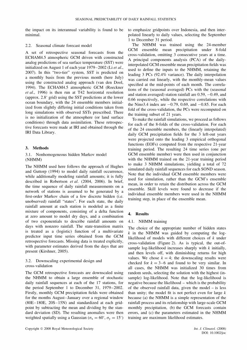
The choice of the appropriate number of hidden statesk in the NHMM was guided by computing the log-likelihood of models with different choices of k undercross-validation (Figure 2). As is typical, the out-of-sample log-likelihood increases sharply with k initially,and then levels off, with diminishing returns for highvalues. We chose k = 4; the downscaling results werechecked for k = 3–6 and found to be very similar. Inall cases, the NHMM was initialized 30 times fromrandom seeds, selecting the solution with the highest (in-sample) log-likelihood. Note that the log-likelihood isnegative because the likelihood – which is the probabilityof the observed rainfall data, given the model – is lessthan unity; the model fit is not perfect even for large k

because (a) the NHMM is a simple representation of therainfall process and its relationship with large-scale GCMmonthly precipitation, (b) the GCM forecasts containerrors, and (c) the parameters estimated in the NHMMtraining are maximum likelihood estimates.



1 2 3 4 5 6 7−8000

−7800

−7600

−7400

−7200

−7000

−6800Cross–validated Log–Likelihood

Number of states

Log–

Like

lihoo

d

Figure 2. Cross-validated log-likelihood as a function of the number ofNHMM states.

4.2. NHMM interpretation

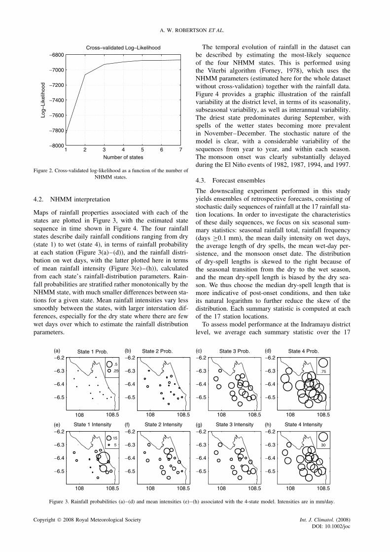
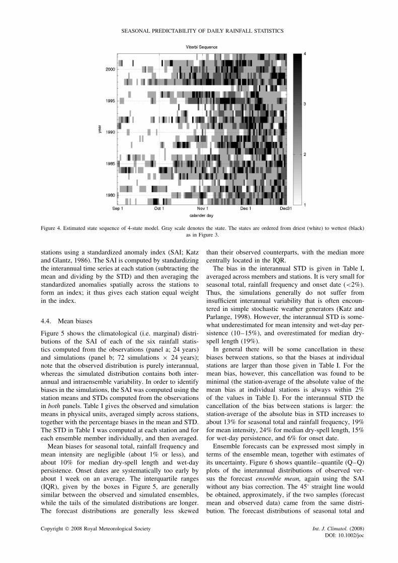
Maps of rainfall properties associated with each of thestates are plotted in Figure 3, with the estimated statesequence in time shown in Figure 4. The four rainfallstates describe daily rainfall conditions ranging from dry(state 1) to wet (state 4), in terms of rainfall probabilityat each station (Figure 3(a)–(d)), and the rainfall distri-bution on wet days, with the latter plotted here in termsof mean rainfall intensity (Figure 3(e)–(h)), calculatedfrom each state’s rainfall-distribution parameters. Rain-fall probabilities are stratified rather monotonically by theNHMM state, with much smaller differences between sta-tions for a given state. Mean rainfall intensities vary lesssmoothly between the states, with larger interstation dif-ferences, especially for the dry state where there are fewwet days over which to estimate the rainfall distributionparameters.

The temporal evolution of rainfall in the dataset canbe described by estimating the most-likely sequenceof the four NHMM states. This is performed usingthe Viterbi algorithm (Forney, 1978), which uses theNHMM parameters (estimated here for the whole datasetwithout cross-validation) together with the rainfall data.Figure 4 provides a graphic illustration of the rainfallvariability at the district level, in terms of its seasonality,subseasonal variability, as well as interannual variability.The driest state predominates during September, withspells of the wetter states becoming more prevalentin November–December. The stochastic nature of themodel is clear, with a considerable variability of thesequences from year to year, and within each season.The monsoon onset was clearly substantially delayedduring the El Nino events of 1982, 1987, 1994, and 1997.

4.3. Forecast ensembles

The downscaling experiment performed in this studyyields ensembles of retrospective forecasts, consisting ofstochastic daily sequences of rainfall at the 17 rainfall sta-tion locations. In order to investigate the characteristicsof these daily sequences, we focus on six seasonal sum-mary statistics: seasonal rainfall total, rainfall frequency(days ≥0.1 mm), the mean daily intensity on wet days,the average length of dry spells, the mean wet-day per-sistence, and the monsoon onset date. The distributionof dry-spell lengths is skewed to the right because ofthe seasonal transition from the dry to the wet season,and the mean dry-spell length is biased by the dry sea-son. We thus choose the median dry-spell length that ismore indicative of post-onset conditions, and then takeits natural logarithm to further reduce the skew of thedistribution. Each summary statistic is computed at eachof the 17 station locations.

To assess model performance at the Indramayu districtlevel, we average each summary statistic over the 17

108 108.5

−6.5

−6.4

−6.3

−6.2

−6.5

−6.4

−6.3

−6.2

−6.5

−6.4

−6.3

−6.2

−6.5

−6.4

−6.3

−6.2

−6.5

−6.4

−6.3

−6.2

−6.5

−6.4

−6.3

−6.2

−6.5

−6.4

−6.3

−6.2

−6.5

−6.4

−6.3

−6.2State 1 Prob.

.5

.25

108 108.5 108 108.5

State 2 Prob. State 3 Prob.

108 108.5

State 4 Prob.

.75

108 108.5

State 1 Intensity

15

5

108.5 108.5108 108 108.5108

State 2 Intensity State 3 Intensity State 4 Intensity

30

(a) (b) (c) (d)

(e) (f) (g) (h)

Figure 3. Rainfall probabilities (a)–(d) and mean intensities (e)–(h) associated with the 4-state model. Intensities are in mm/day.



Figure 4. Estimated state sequence of 4-state model. Gray scale denotes the state. The states are ordered from driest (white) to wettest (black)as in Figure 3.

stations using a standardized anomaly index (SAI; Katzand Glantz, 1986). The SAI is computed by standardizingthe interannual time series at each station (subtracting themean and dividing by the STD) and then averaging thestandardized anomalies spatially across the stations toform an index; it thus gives each station equal weightin the index.

4.4. Mean biases

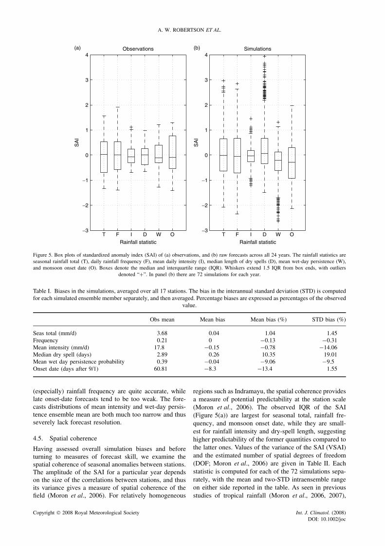
Figure 5 shows the climatological (i.e. marginal) distri-butions of the SAI of each of the six rainfall statis-tics computed from the observations (panel a; 24 years)and simulations (panel b; 72 simulations × 24 years);note that the observed distribution is purely interannual,whereas the simulated distribution contains both inter-annual and intraensemble variability. In order to identifybiases in the simulations, the SAI was computed using thestation means and STDs computed from the observationsin both panels. Table I gives the observed and simulationmeans in physical units, averaged simply across stations,together with the percentage biases in the mean and STD.The STD in Table I was computed at each station and foreach ensemble member individually, and then averaged.

Mean biases for seasonal total, rainfall frequency andmean intensity are negligible (about 1% or less), andabout 10% for median dry-spell length and wet-daypersistence. Onset dates are systematically too early byabout 1 week on an average. The interquartile ranges(IQR), given by the boxes in Figure 5, are generallysimilar between the observed and simulated ensembles,while the tails of the simulated distributions are longer.The forecast distributions are generally less skewed

than their observed counterparts, with the median morecentrally located in the IQR.

The bias in the interannual STD is given in Table I,averaged across members and stations. It is very small forseasonal total, rainfall frequency and onset date (<2%).Thus, the simulations generally do not suffer frominsufficient interannual variability that is often encoun-tered in simple stochastic weather generators (Katz andParlange, 1998). However, the interannual STD is some-what underestimated for mean intensity and wet-day per-sistence (10–15%), and overestimated for median dry-spell length (19%).

In general there will be some cancellation in thesebiases between stations, so that the biases at individualstations are larger than those given in Table I. For themean bias, however, this cancellation was found to beminimal (the station-average of the absolute value of themean bias at individual stations is always within 2%of the values in Table I). For the interannual STD thecancellation of the bias between stations is larger: thestation-average of the absolute bias in STD increases toabout 13% for seasonal total and rainfall frequency, 19%for mean intensity, 24% for median dry-spell length, 15%for wet-day persistence, and 6% for onset date.

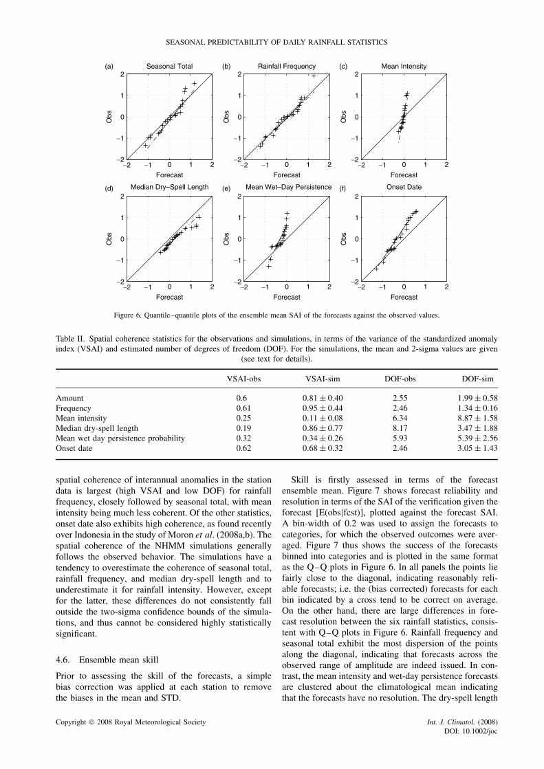
Ensemble forecasts can be expressed most simply interms of the ensemble mean, together with estimates ofits uncertainty. Figure 6 shows quantile–quantile (Q–Q)plots of the interannual distributions of observed ver-sus the forecast ensemble mean, again using the SAIwithout any bias correction. The 45° straight line wouldbe obtained, approximately, if the two samples (forecastmean and observed data) came from the same distri-bution. The forecast distributions of seasonal total and



T F I D W O

Rainfall statistic

T F I D W O

Rainfall statistic

Observations Simulations

−3

−2

−1

0

1

2

3

4

SA

I

(a)

−3

−2

−1

0

1

2

3

4

SA

I

(b)

Figure 5. Box plots of standardized anomaly index (SAI) of (a) observations, and (b) raw forecasts across all 24 years. The rainfall statistics areseasonal rainfall total (T), daily rainfall frequency (F), mean daily intensity (I), median length of dry spells (D), mean wet-day persistence (W),and monsoon onset date (O). Boxes denote the median and interquartile range (IQR). Whiskers extend 1.5 IQR from box ends, with outliers

denoted “+”. In panel (b) there are 72 simulations for each year.

Table I. Biases in the simulations, averaged over all 17 stations. The bias in the interannual standard deviation (STD) is computedfor each simulated ensemble member separately, and then averaged. Percentage biases are expressed as percentages of the observed

value.

Obs mean Mean bias Mean bias (%) STD bias (%)

Seas total (mm/d) 3.68 0.04 1.04 1.45Frequency 0.21 0 −0.13 −0.31Mean intensity (mm/d) 17.8 −0.15 −0.78 −14.06Median dry spell (days) 2.89 0.26 10.35 19.01Mean wet day persistence probability 0.39 −0.04 −9.06 −9.5Onset date (days after 9/1) 60.81 −8.3 −13.4 1.55

(especially) rainfall frequency are quite accurate, whilelate onset-date forecasts tend to be too weak. The fore-casts distributions of mean intensity and wet-day persis-tence ensemble mean are both much too narrow and thusseverely lack forecast resolution.

4.5. Spatial coherence

Having assessed overall simulation biases and beforeturning to measures of forecast skill, we examine thespatial coherence of seasonal anomalies between stations.The amplitude of the SAI for a particular year dependson the size of the correlations between stations, and thusits variance gives a measure of spatial coherence of thefield (Moron et al., 2006). For relatively homogeneous

regions such as Indramayu, the spatial coherence providesa measure of potential predictability at the station scale(Moron et al., 2006). The observed IQR of the SAI(Figure 5(a)) are largest for seasonal total, rainfall fre-quency, and monsoon onset date, while they are small-est for rainfall intensity and dry-spell length, suggestinghigher predictability of the former quantities compared tothe latter ones. Values of the variance of the SAI (VSAI)and the estimated number of spatial degrees of freedom(DOF; Moron et al., 2006) are given in Table II. Eachstatistic is computed for each of the 72 simulations sepa-rately, with the mean and two-STD intraensemble rangeon either side reported in the table. As seen in previousstudies of tropical rainfall (Moron et al., 2006, 2007),



−2

Seasonal Total Rainfall Frequency Mean Intensity

Median Dry–Spell Length

−1 0 1 2−2

−1

0

1

2

Obs

Forecast

(a)

−1 0 1 2−2

−1

0

1

2

Obs

Forecast

(d) Mean Wet–Day Persistence

−1 0 1 2−2

−1

0

1

2

Obs

Forecast

(e) Onset Date

−1 0 1 2−2

−1

0

1

2

Obs

Forecast

(f)

−1 0 1 2−2

−1

0

1

2

Obs

Forecast

(b)

−1 0 1 2−2

−1

0

1

2

Obs

Forecast

(c)

−2

−2−2

−2

−2

Figure 6. Quantile–quantile plots of the ensemble mean SAI of the forecasts against the observed values.

Table II. Spatial coherence statistics for the observations and simulations, in terms of the variance of the standardized anomalyindex (VSAI) and estimated number of degrees of freedom (DOF). For the simulations, the mean and 2-sigma values are given

(see text for details).

VSAI-obs VSAI-sim DOF-obs DOF-sim

Amount 0.6 0.81 ± 0.40 2.55 1.99 ± 0.58Frequency 0.61 0.95 ± 0.44 2.46 1.34 ± 0.16Mean intensity 0.25 0.11 ± 0.08 6.34 8.87 ± 1.58Median dry-spell length 0.19 0.86 ± 0.77 8.17 3.47 ± 1.88Mean wet day persistence probability 0.32 0.34 ± 0.26 5.93 5.39 ± 2.56Onset date 0.62 0.68 ± 0.32 2.46 3.05 ± 1.43

spatial coherence of interannual anomalies in the stationdata is largest (high VSAI and low DOF) for rainfallfrequency, closely followed by seasonal total, with meanintensity being much less coherent. Of the other statistics,onset date also exhibits high coherence, as found recentlyover Indonesia in the study of Moron et al. (2008a,b). Thespatial coherence of the NHMM simulations generallyfollows the observed behavior. The simulations have atendency to overestimate the coherence of seasonal total,rainfall frequency, and median dry-spell length and tounderestimate it for rainfall intensity. However, exceptfor the latter, these differences do not consistently falloutside the two-sigma confidence bounds of the simula-tions, and thus cannot be considered highly statisticallysignificant.

4.6. Ensemble mean skill

Prior to assessing the skill of the forecasts, a simplebias correction was applied at each station to removethe biases in the mean and STD.

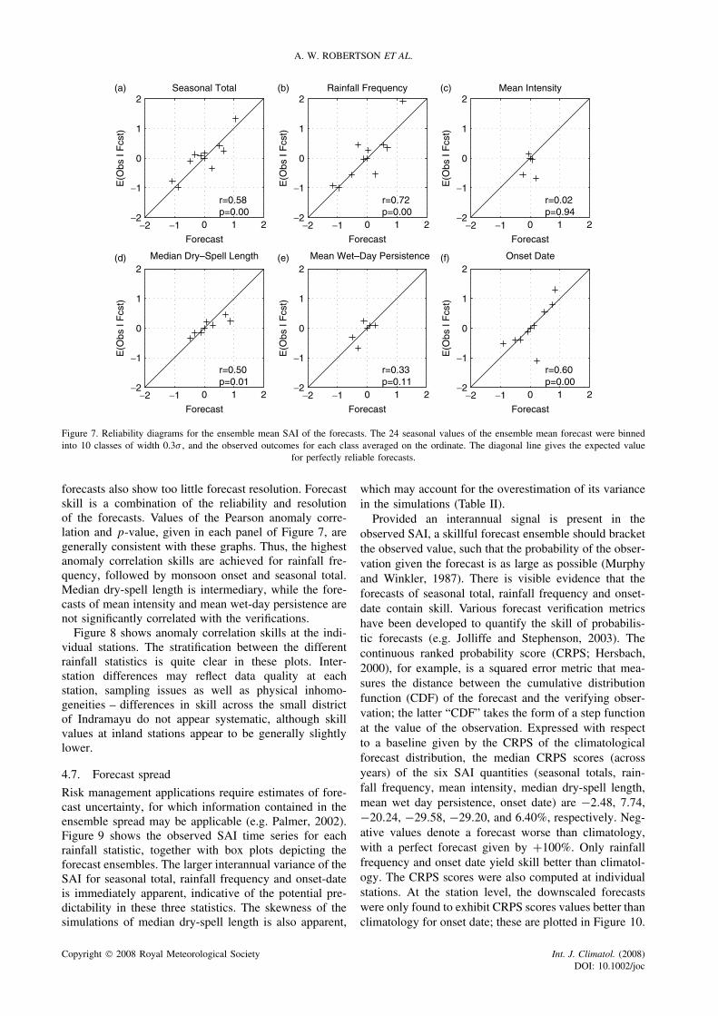
Skill is firstly assessed in terms of the forecastensemble mean. Figure 7 shows forecast reliability andresolution in terms of the SAI of the verification given theforecast [E(obs|fcst)], plotted against the forecast SAI.A bin-width of 0.2 was used to assign the forecasts tocategories, for which the observed outcomes were aver-aged. Figure 7 thus shows the success of the forecastsbinned into categories and is plotted in the same formatas the Q–Q plots in Figure 6. In all panels the points liefairly close to the diagonal, indicating reasonably reli-able forecasts; i.e. the (bias corrected) forecasts for eachbin indicated by a cross tend to be correct on average.On the other hand, there are large differences in fore-cast resolution between the six rainfall statistics, consis-tent with Q–Q plots in Figure 6. Rainfall frequency andseasonal total exhibit the most dispersion of the pointsalong the diagonal, indicating that forecasts across theobserved range of amplitude are indeed issued. In con-trast, the mean intensity and wet-day persistence forecastsare clustered about the climatological mean indicatingthat the forecasts have no resolution. The dry-spell length



−2

−2 −2 −2

−2 −2


Median Dry–Spell Length

−1 0 1 2−2

−1

0

1

2

E(O

bs I

Fcs

t)

Forecast

(a)

−1 0 1 2−2

−1

0

1

2

E(O

bs I

Fcs

t)

Forecast

(d) Mean Wet–Day Persistence

−1 0 1 2−2

−1

0

1

2E

(Obs

I F

cst)

Forecast

(e) Onset Date

−1 0 1 2−2

−1

0

1

2

E(O

bs I

Fcs

t)

Forecast

(f)

−1 0 1 2−2

−1

0

1

2

E(O

bs I

Fcs

t)

Forecast

(b)

−1 0 1 2−2

−1

0

1

2

E(O

bs I

Fcs

t)

Forecast

(c)

r=0.58p=0.00

r=0.72p=0.00

r=0.02p=0.94

r=0.50p=0.01

r=0.33p=0.11

r=0.60p=0.00

Figure 7. Reliability diagrams for the ensemble mean SAI of the forecasts. The 24 seasonal values of the ensemble mean forecast were binnedinto 10 classes of width 0.3σ , and the observed outcomes for each class averaged on the ordinate. The diagonal line gives the expected value

for perfectly reliable forecasts.

forecasts also show too little forecast resolution. Forecastskill is a combination of the reliability and resolutionof the forecasts. Values of the Pearson anomaly corre-lation and p-value, given in each panel of Figure 7, aregenerally consistent with these graphs. Thus, the highestanomaly correlation skills are achieved for rainfall fre-quency, followed by monsoon onset and seasonal total.Median dry-spell length is intermediary, while the fore-casts of mean intensity and mean wet-day persistence arenot significantly correlated with the verifications.

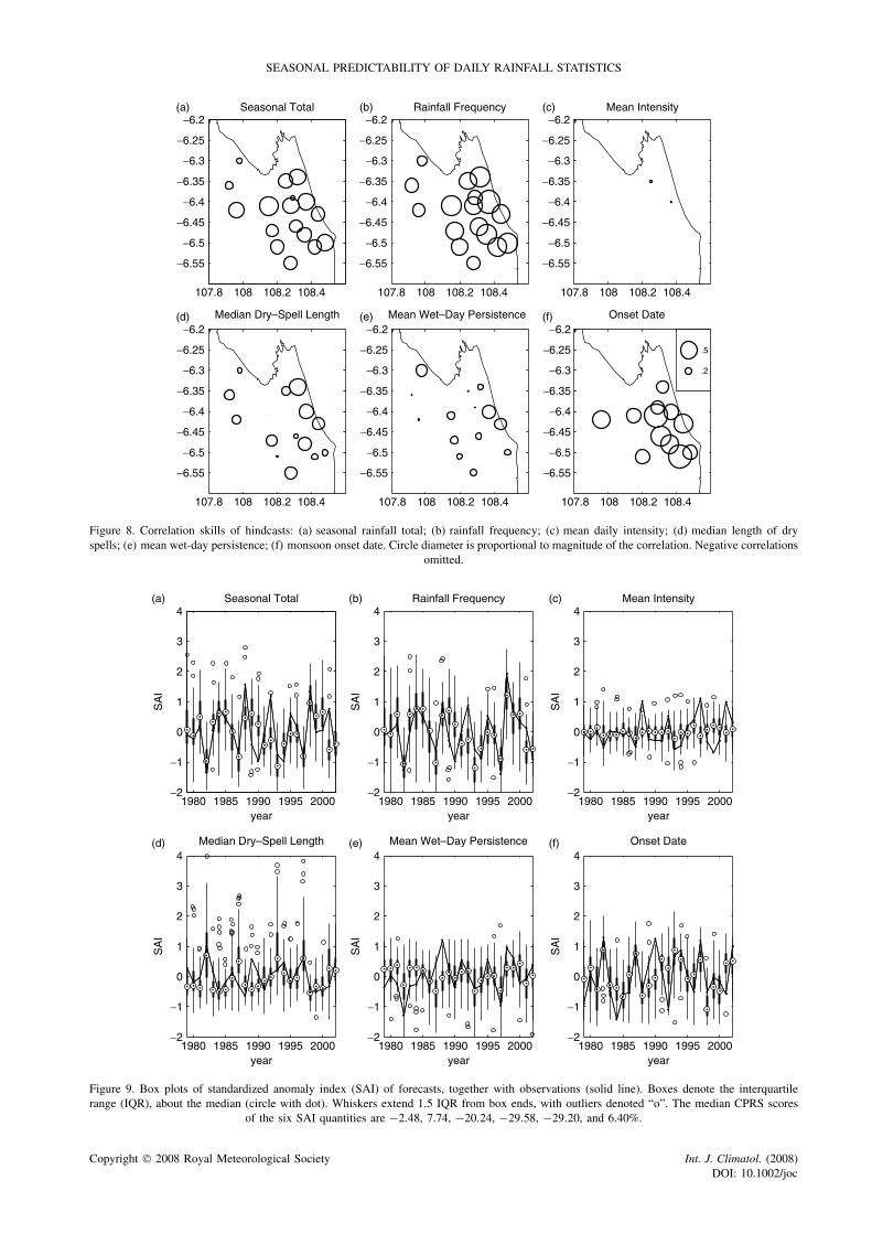
Figure 8 shows anomaly correlation skills at the indi-vidual stations. The stratification between the differentrainfall statistics is quite clear in these plots. Inter-station differences may reflect data quality at eachstation, sampling issues as well as physical inhomo-geneities – differences in skill across the small districtof Indramayu do not appear systematic, although skillvalues at inland stations appear to be generally slightlylower.

4.7. Forecast spread

Risk management applications require estimates of fore-cast uncertainty, for which information contained in theensemble spread may be applicable (e.g. Palmer, 2002).Figure 9 shows the observed SAI time series for eachrainfall statistic, together with box plots depicting theforecast ensembles. The larger interannual variance of theSAI for seasonal total, rainfall frequency and onset-dateis immediately apparent, indicative of the potential pre-dictability in these three statistics. The skewness of thesimulations of median dry-spell length is also apparent,

which may account for the overestimation of its variancein the simulations (Table II).

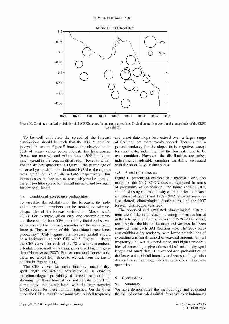
Provided an interannual signal is present in theobserved SAI, a skillful forecast ensemble should bracketthe observed value, such that the probability of the obser-vation given the forecast is as large as possible (Murphyand Winkler, 1987). There is visible evidence that theforecasts of seasonal total, rainfall frequency and onset-date contain skill. Various forecast verification metricshave been developed to quantify the skill of probabilis-tic forecasts (e.g. Jolliffe and Stephenson, 2003). Thecontinuous ranked probability score (CRPS; Hersbach,2000), for example, is a squared error metric that mea-sures the distance between the cumulative distributionfunction (CDF) of the forecast and the verifying obser-vation; the latter “CDF” takes the form of a step functionat the value of the observation. Expressed with respectto a baseline given by the CRPS of the climatologicalforecast distribution, the median CRPS scores (acrossyears) of the six SAI quantities (seasonal totals, rain-fall frequency, mean intensity, median dry-spell length,mean wet day persistence, onset date) are −2.48, 7.74,−20.24, −29.58, −29.20, and 6.40%, respectively. Neg-ative values denote a forecast worse than climatology,with a perfect forecast given by +100%. Only rainfallfrequency and onset date yield skill better than climatol-ogy. The CRPS scores were also computed at individualstations. At the station level, the downscaled forecastswere only found to exhibit CRPS scores values better thanclimatology for onset date; these are plotted in Figure 10.



107.8 108 108.2 108.4

−6.55

−6.5

−6.45

−6.4

−6.35

−6.3

−6.25

−6.2

107.8 108 108.2 108.4

−6.55

−6.5

−6.45

−6.4

−6.35

−6.3

−6.25

−6.2Seasonal Total Rainfall Frequency Mean Intensity

Median Dry–Spell Length Mean Wet–Day Persistence Onset Date

.5

.2

.5

107.8 108 108.2 108.4

−6.55

−6.5

−6.45

−6.4

−6.35

−6.3

−6.25

−6.2(a)

107.8 108 108.2 108.4

−6.55

−6.5

−6.45

−6.4

−6.35

−6.3

−6.25

−6.2(d)

107.8 108 108.2 108.4

−6.55

−6.5

−6.45

−6.4

−6.35

−6.3

−6.25

−6.2(e)

107.8 108 108.2 108.4

−6.55

−6.5

−6.45

−6.4

−6.35

−6.3

−6.25

−6.2(f)

(b) (c)

Figure 8. Correlation skills of hindcasts: (a) seasonal rainfall total; (b) rainfall frequency; (c) mean daily intensity; (d) median length of dryspells; (e) mean wet-day persistence; (f) monsoon onset date. Circle diameter is proportional to magnitude of the correlation. Negative correlations

omitted.

1980 1985 1990 1995 2000−2

−1

0

1

2

3

4

SA

I

year1980 1985 1990 1995 2000

−2

−1

0

1

2

3

4

SA

I

year



1980 1985 1990 1995 2000−2

−1

0

1

2

3

4

SA

I

year

(a)

1980 1985 1990 1995 2000−2

−1

0

1

2

3

4

SA

I

year

(d)

1980 1985 1990 1995 2000−2

−1

0

1

2

3

4

SA

I

year

(e)

1980 1985 1990 1995 2000−2

−1

0

1

2

3

4

SA

I

year

(f)

(b) (c)

Figure 9. Box plots of standardized anomaly index (SAI) of forecasts, together with observations (solid line). Boxes denote the interquartilerange (IQR), about the median (circle with dot). Whiskers extend 1.5 IQR from box ends, with outliers denoted “o”. The median CPRS scores

of the six SAI quantities are −2.48, 7.74, −20.24, −29.58, −29.20, and 6.40%.



107.8 107.9 108 108.1 108.2 108.3 108.4 108.5 108.6

Median CRPSS Onset Date

25%

10%

−6.55

−6.5

−6.45

−6.4

−6.35

−6.3

−6.25

−6.2

Figure 10. Continuous ranked probability skill (CRPS) scores for monsoon onset date. Circle diameter is proportional to magnitude of the CRPSscore (in %).

To be well calibrated, the spread of the forecastdistributions should be such that the IQR “predictioninterval” boxes in Figure 9 bracket the observation in50% of years; values below indicate too little spread(boxes too narrow), and values above 50% imply toomuch spread in the forecast distribution (boxes to wide).For the six SAI quantities in Figure 9, the percentage ofobserved years within the simulated IQR (i.e. the capturerates) are 58, 62, 37, 71, 46, and 46% respectively. Thusin most cases the forecasts are reasonably well calibrated;there is too little spread for rainfall intensity and too muchfor dry-spell length.

4.8. Conditional exceedance probabilities

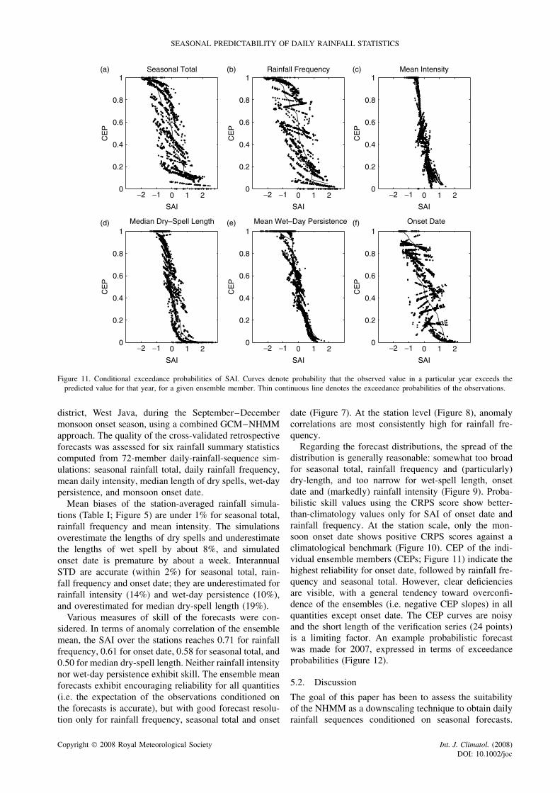
To visualize the reliability of the forecasts, the indi-vidual ensemble members can be treated as estimatesof quantiles of the forecast distribution (Mason et al.,2007). For example, given only one ensemble mem-ber, there should be a 50% probability that the observedvalue exceeds the forecast, regardless of the value beingforecast. Thus, a graph of this “conditional exceedanceprobability” (CEP) against the forecast rainfall shouldbe a horizontal line with CEP = 0.5. Figure 11 showsthe CEP curves for each of the 72 ensemble members,calculated across all years using generalized linear regres-sion (Mason et al., 2007). For seasonal total, for example,these are ranked from driest to wettest, from the top tobottom in Figure 11(a).

The CEP curves for mean intensity, median dry-spell length and wet-day persistence all lie close tothe climatological probability of exceedance (thin line),showing that these forecasts do not deviate much fromclimatology; this is consistent with the large negativeCPRS scores for these rainfall statistics. On the otherhand, the CEP curves for seasonal total, rainfall frequency

and onset date slope less extend over a larger rangeof SAI and are more evenly spaced. There is still ageneral tendency for the slopes to be negative, exceptfor onset date, indicating that the forecasts tend to beover confident. However, the distributions are noisy,indicating considerable sampling variability associatedwith the short 24-year time series.

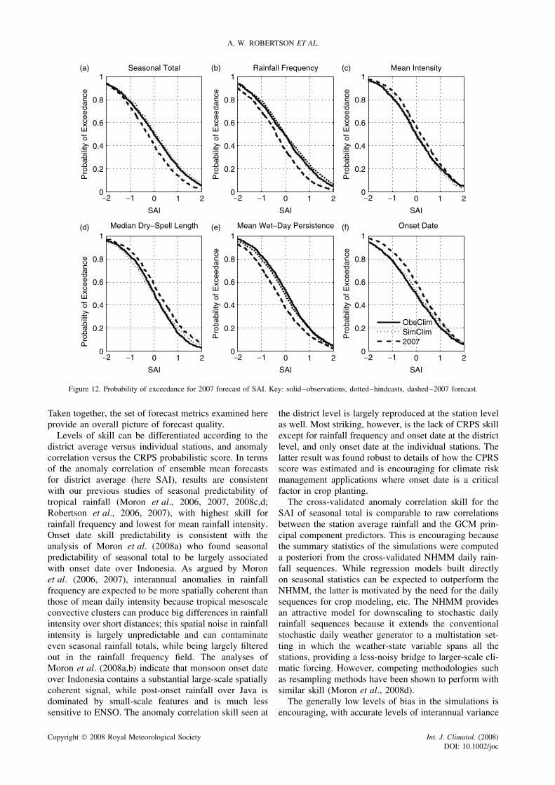
4.9. A real-time forecastFigure 12 presents an example of a forecast distributionmade for the 2007 SOND season, expressed in termsof probability of exceedance. The figure shows CDFs,smoothed using a kernel density estimator, for the histor-ical observed (solid) and 1979–2002 retrospective fore-cast (dotted) climatological distributions, and the 2007forecast distribution (dashed).

The observed and simulated climatological distribu-tions are similar in all cases indicating no serious biasesin the retrospective forecasts over the 1979–2002 period,recalling that the bias in the mean and variance has beenremoved from each SAI (Section 4.6). The 2007 fore-cast exhibits a dry tendency, with lower probabilities ofexceeding a given threshold of seasonal amount, rainfallfrequency, and wet-day persistence, and higher probabil-ities of exceeding a given threshold of median dry-spelllength and onset date. The exceedance probabilities ofthe forecast for rainfall intensity and wet-spell length alsodeviate from climatology, despite the lack of skill in thesequantities.

5. Conclusions

5.1. SummaryWe have demonstrated the methodology and evaluatedthe skill of downscaled rainfall forecasts over Indramayu





−2 −1 0 1 20

0.2

0.4

0.6

0.8

1

SAI

CE

P

(a)

−2 −1 0 1 20

0.2

0.4

0.6

0.8

1

SAI

CE

P

(d)

−2 −1 0 1 20

0.2

0.4

0.6

0.8

1

SAI

CE

P

(b)

−2 −1 0 1 20

0.2

0.4

0.6

0.8

1

SAI

CE

P(e)

−2 −1 0 1 20

0.2

0.4

0.6

0.8

1

SAIC

EP

(f)

−2 −1 0 1 20

0.2

0.4

0.6

0.8

1

SAI

CE

P

(c)

Figure 11. Conditional exceedance probabilities of SAI. Curves denote probability that the observed value in a particular year exceeds thepredicted value for that year, for a given ensemble member. Thin continuous line denotes the exceedance probabilities of the observations.

district, West Java, during the September–Decembermonsoon onset season, using a combined GCM–NHMMapproach. The quality of the cross-validated retrospectiveforecasts was assessed for six rainfall summary statisticscomputed from 72-member daily-rainfall-sequence sim-ulations: seasonal rainfall total, daily rainfall frequency,mean daily intensity, median length of dry spells, wet-daypersistence, and monsoon onset date.

Mean biases of the station-averaged rainfall simula-tions (Table I; Figure 5) are under 1% for seasonal total,rainfall frequency and mean intensity. The simulationsoverestimate the lengths of dry spells and underestimatethe lengths of wet spell by about 8%, and simulatedonset date is premature by about a week. InterannualSTD are accurate (within 2%) for seasonal total, rain-fall frequency and onset date; they are underestimated forrainfall intensity (14%) and wet-day persistence (10%),and overestimated for median dry-spell length (19%).

Various measures of skill of the forecasts were con-sidered. In terms of anomaly correlation of the ensemblemean, the SAI over the stations reaches 0.71 for rainfallfrequency, 0.61 for onset date, 0.58 for seasonal total, and0.50 for median dry-spell length. Neither rainfall intensitynor wet-day persistence exhibit skill. The ensemble meanforecasts exhibit encouraging reliability for all quantities(i.e. the expectation of the observations conditioned onthe forecasts is accurate), but with good forecast resolu-tion only for rainfall frequency, seasonal total and onset

date (Figure 7). At the station level (Figure 8), anomalycorrelations are most consistently high for rainfall fre-quency.

Regarding the forecast distributions, the spread of thedistribution is generally reasonable: somewhat too broadfor seasonal total, rainfall frequency and (particularly)dry-length, and too narrow for wet-spell length, onsetdate and (markedly) rainfall intensity (Figure 9). Proba-bilistic skill values using the CRPS score show better-than-climatology values only for SAI of onset date andrainfall frequency. At the station scale, only the mon-soon onset date shows positive CRPS scores against aclimatological benchmark (Figure 10). CEP of the indi-vidual ensemble members (CEPs; Figure 11) indicate thehighest reliability for onset date, followed by rainfall fre-quency and seasonal total. However, clear deficienciesare visible, with a general tendency toward overconfi-dence of the ensembles (i.e. negative CEP slopes) in allquantities except onset date. The CEP curves are noisyand the short length of the verification series (24 points)is a limiting factor. An example probabilistic forecastwas made for 2007, expressed in terms of exceedanceprobabilities (Figure 12).

5.2. Discussion

The goal of this paper has been to assess the suitabilityof the NHMM as a downscaling technique to obtain dailyrainfall sequences conditioned on seasonal forecasts.





−2 −1 0 1 2

−2 −1 0 1 2 −2 −1 0 1 2 −2 −1 0 1 2

−2 −1 0 1 2 −2 −1 0 1 20

0.2

0.4

0.6

0.8

1

SAI

Pro

babi

lity

of E

xcee

danc

e

(a)

0

0.2

0.4

0.6

0.8

1

SAI

Pro

babi

lity

of E

xcee

danc

e

(d)

0

0.2

0.4

0.6

0.8

1

SAIP

roba

bilit

y of

Exc

eeda

nce

(b)

0

0.2

0.4

0.6

0.8

1

SAI

Pro

babi

lity

of E

xcee

danc

e

(e)

0

0.2

0.4

0.6

0.8

1

SAI

Pro

babi

lity

of E

xcee

danc

e

(f)

0

0.2

0.4

0.6

0.8

1

SAI

Pro

babi

lity

of E

xcee

danc

e

(c)

2007SimClimObsClim

Figure 12. Probability of exceedance for 2007 forecast of SAI. Key: solid–observations, dotted–hindcasts, dashed–2007 forecast.

Taken together, the set of forecast metrics examined hereprovide an overall picture of forecast quality.

Levels of skill can be differentiated according to thedistrict average versus individual stations, and anomalycorrelation versus the CRPS probabilistic score. In termsof the anomaly correlation of ensemble mean forecastsfor district average (here SAI), results are consistentwith our previous studies of seasonal predictability oftropical rainfall (Moron et al., 2006, 2007, 2008c,d;Robertson et al., 2006, 2007), with highest skill forrainfall frequency and lowest for mean rainfall intensity.Onset date skill predictability is consistent with theanalysis of Moron et al. (2008a) who found seasonalpredictability of seasonal total to be largely associatedwith onset date over Indonesia. As argued by Moronet al. (2006, 2007), interannual anomalies in rainfallfrequency are expected to be more spatially coherent thanthose of mean daily intensity because tropical mesoscaleconvective clusters can produce big differences in rainfallintensity over short distances; this spatial noise in rainfallintensity is largely unpredictable and can contaminateeven seasonal rainfall totals, while being largely filteredout in the rainfall frequency field. The analyses ofMoron et al. (2008a,b) indicate that monsoon onset dateover Indonesia contains a substantial large-scale spatiallycoherent signal, while post-onset rainfall over Java isdominated by small-scale features and is much lesssensitive to ENSO. The anomaly correlation skill seen at

the district level is largely reproduced at the station levelas well. Most striking, however, is the lack of CRPS skillexcept for rainfall frequency and onset date at the districtlevel, and only onset date at the individual stations. Thelatter result was found robust to details of how the CPRSscore was estimated and is encouraging for climate riskmanagement applications where onset date is a criticalfactor in crop planting.

The cross-validated anomaly correlation skill for theSAI of seasonal total is comparable to raw correlationsbetween the station average rainfall and the GCM prin-cipal component predictors. This is encouraging becausethe summary statistics of the simulations were computeda posteriori from the cross-validated NHMM daily rain-fall sequences. While regression models built directlyon seasonal statistics can be expected to outperform theNHMM, the latter is motivated by the need for the dailysequences for crop modeling, etc. The NHMM providesan attractive model for downscaling to stochastic dailyrainfall sequences because it extends the conventionalstochastic daily weather generator to a multistation set-ting in which the weather-state variable spans all thestations, providing a less-noisy bridge to larger-scale cli-matic forcing. However, competing methodologies suchas resampling methods have been shown to perform withsimilar skill (Moron et al., 2008d).

The generally low levels of bias in the simulations isencouraging, with accurate levels of interannual variance



for the more skillful quantities, i.e. onset date, seasonaltotal and rainfall frequency. However, the mean onsetdate of the simulations is premature by about 1 week.This is probably largely due to biases in the GCM predic-tors since use of reanalysis-based predictors was largelyable to remove this bias (not shown). Further work isrequired to address this issue, before the GCM–NHMMsimulated daily rainfall sequences could be used to drivecrop models, for example, which may be sensitive to tim-ing of rainy season onset. Our results are likely to betypical of what might be expected for downscaling overother areas of Indonesia where the large-scale climate sig-nal in onset is pronounced, such as Sumatra, Java, NusaTengara, and Timor.

Acknowledgements

We are grateful to Rizaldi Boer for assistance with therainfall station data, and to Sergey Kirshner, SimonMason, and Padhraic Smyth for helpful discussions.The NHMM software (MVNHMM) was developed byS. Kirshner and can be obtained free of charge fromhttp://www.stat.purdue.edu/∼skirshne/MVNHMM/. Thisresearch was supported by grants from the NationalOceanic and Atmospheric Administration (NOAA),NA050AR4311004, the US Agency for InternationalDevelopment’s Office of Foreign Disaster Assistance,DFD-A-00-03-00005-00, and the US Department ofEnergy’s Climate Change Prediction Program, DE-FG02-02ER63413. The computing for this project was partiallyprovided by a grant from the NCAR CSL program tothe IRI.

References

Aldrian E, Dumenil-Gates L, Widodo FH. 2007. Seasonal variability ofIndonesian rainfall in ECHAM4 simulations and in the reanalyses:the role of ENSO. Theoretical and Applied Climatology 87:41–59.

Aldrian E, Sein D, Jacob D, Dumenil-Gates L, Podzun R. 2005.Modeling Indonesian rainfall with a coupled regional model. ClimateDynamics 25: 1–17.

Aldrian E, Susanto RD. 2003. Identification of three dominantrainfall regions within Indonesia and their relationship to seasurface temperature. International Journal of Climatology 23:1435–1452.

Boer R, Wahab I. 2007. Use of seasonal surface temperature forpredicting optimum planting window for potato at Pengalengan, WestJava, Indonesia. In Climate Prediction and Agriculture: Advance andChallenge, Sivakumar MVK, Hansen J (eds). Springer: New York;135–141.

Charles SP, Bates BC, Smith IN, Hughes JP. 2004. Statisticaldownscaling from observed and modelled atmospheric fields.Hydrological Processes 18: 1373–1394.

Charles SP, Bates BC, Viney NR. 2003. Linking atmosphericcirculation to daily rainfall patterns across the Murrumbidgee RiverBasin. Water Science Technology 48: 233–240.

Forney GD Jr. 1978. The Viterbi algorithm. Proceedings of the IEEE61: 268–278.

Goddard L, Mason SJ, Zebiak SE, Ropelewski CF, Basher R,Cane MA. 2001. Current approaches to seasonal-to-interannualclimate predictions. International Journal of Climatology 21:1111–1152.

Gong X, Barnston AG, Ward MN. 2003. The effect of spa-tial aggregation on the skill of seasonal precipitation fore-casts. Journal of Climate 16: 3059–3071, DOI: 10.1175/1520-0442(2003)016<3059:TEOSAO>2.0.CO;2.

Giannini A, Robertson AW, Qian JH. 2007. A role for tropical tropo-spheric temperature adjustment to ENSO in the seasonality of mon-soonal Indonesia precipitation predictability. Journal of GeophysicalResearch-Atmospheres 112: D16110, DOI:10.1029/2007JD008519.

Hamada JI, Yamanaka MD, Matsumoto J, Fukao S, Winarso PA,Sribimawati T. 2002. Spatial and temporal variations of the rainyseason over Indonesia and their link to ENSO. Journal of theMeteorological Society of Japan 80: 285–310.

Hansen JW, Ines AVM. 2005. Stochastic disaggregation of monthlyrainfall data for crop simulation studies. Agricultural and ForestMeteorology 131: 233–246.

Haylock M, McBride J. 2001. Spatial coherence and predictabilityof Indonesian wet season rainfall. Journal of Climate 14:3882–3887.

Hersbach H. 2000. Decomposition of the Continuous RankedProbability Score for ensemble prediction systems. Weather andForecasting 15: 559–570.

Hughes JP, Guttorp P. 1994. A class of stochastic models for relatingsynoptic atmospheric patterns to regional hydrologic phenomena.Water Resources Research 30: 1535–1546.

Ines AVM, Hansen JW. 2006. Bias correction of daily GCM rainfall forcrop simulation studies. Agricultural and Forest Meteorology 138:44–53.

Jolliffe IT, Stephenson DB (eds). 2003. Forecast Verification: APractitioner’s Guide in Atmospheric Science. John Wiley and Sons:Chichester, ISBN 0-471-49759-2.

Juneng L, Tangang FT. 2005. Evolution of ENSO-related rainfallanomalies in Southeast Asia region and its relationship withatmosphere-ocean variations in Indo-Pacific sector. ClimateDynamics 25: 337–350.

Katz RW, Glantz MH. 1986. Anatomy of a rainfall index. MonthlyWeather Review 114: 764–771.

Katz RW, Parlange MB. 1998. Overdispersion phenomenon instochastic modeling of precipitation. Journal of Climate 11:591–601.

Kirshner, S. 2005. Modeling of multivariate time series using hiddenMarkov models. Ph.D. thesis, University of California, Irvine.

Li S, Goddard L, DeWitt DG. 2007. Predictive skill of AGCM seasonalclimate forecasts subject to different SST prediction methodologies.Journal of Climate 21: 2169–2186.

Mason SJ, Galpin JS, Goddard L, Graham NE, Rajartnam B. 2007.Conditional exceedance probabilities. Monthly Weather Review 135:363–372.

Moron V, Robertson AW, Boer R. 2008a. Spatial coherence andseasonal predictability of monsoon onset over Indonesia. Journalof Climate (in press).

Moron V, Robertson AW, Qian J-H. 2008b. Local versus large-scalecharacteristics of monsoon onset and post-onset rainfall overIndonesia. Climate Dynamics sub judice. (in review).

Moron V, Robertson AW, Ward MN. 2008c. Weather types and rainfallover senegal. Part I: observational analysis. Journal of Climate 21:266–287.

Moron V, Robertson AW, Ward MN. 2008d. Weather types and rainfallin Senegal. Part II: Downscaling of GCM Simulations. Journal ofClimate 21: 288–307.

Moron V, Robertson AW, Ward MN. 2006. Seasonal predictability andspatial coherence of rainfall characteristics in the tropical setting ofSenegal. Monthly Weather Review 134: 3468–3482.

Moron V, Robertson AW, Ward MN, Camberlin P. 2007. Spatialcoherence of tropical rainfall at regional scale. Journal of Climate20: 5244–5263.

Murphy AH, Winkler RL. 1987. A general framework for forecastverification. Monthly Weather Review 115: 1330–1338.

Naylor RL, Falcon W, Wada N, Rochberg D. 2002. Using El-Nino Southern Oscillation climate data to improve food policyplanning in Indonesia. Bulletin of Indonesian Economic Studies 38:75–91.

Palmer TN. 2002. The economic value of ensemble forecasts as a toolfor risk assessment: From days to decades. Quarterly Journal of theRoyal Meteorological Society 128: 747–774.

Robertson AW, Ines AVM, Hansen JW. 2007. Downscaling ofseasonal precipitation for crop simulation. Journal of AppliedMeteorology and Climatology 46: 677–693.

Robertson AW, Kirshner S, Smyth P. 2004. Downscaling of dailyrainfall occurrence over Northeast Brazil using a Hidden MarkovModel. Journal of Climate 17: 4407–4424.

Robertson AW, Kirshner S, Smyth P, Charles SP, Bates BC. 2006.Subseasonal-to-interdecadal variability of the Australian monsoon



over North Queensland. Quarterly Journal of the Royal Meteorolog-ical Society 132: 519–542.

Roeckner E, Arpe K, Bengtsson L, Christoph M, Claussen M, Dume-nil L, Esch M, Giorgetta M, Schlese U, Schulzweida U. 1996. Theatmospheric general circulation model ECHAM4: Model descrip-tion and simulation of present-day climate. Technical Report218. Max Planck Institute for Meteorology: Hamburg, Germany;90.

Sivakumar MVK. 1988. Predicting rainy season potential from theonset of rains in southern Sahelian and Sudanian climatic zones ofWest Africa. Agricultural and Forest Meteorology 42: 295–305.

van den Dool HM. 1994. Searching for analogues, how long must wewait? Tellus 46A: 314–324.

Wilks DS. 1999. Interannual variability and extreme-value character-istics of several stochastic daily precipitation models. Agriculturaland Forest Meteorology 93: 153–169.


Documents

Seasonal predictability of daily rainfall statistics over ...awr/TP/Indonesia/Papers/RobertsonMoronSwarinoto_IJC08.pdf · Seasonal predictability of daily rainfall statistics over