Seasonality of climate–human mortality relationships in US ... · Seasonality of climate–human mortality relationships in US cities and impacts of climate ... tionships between

CLIMATE RESEARCHClim Res

Vol. 26: 61–76, 2004 Published April 19

1. INTRODUCTION

Future increases in human-mortality rates areamong the suite of potential impacts expected to arisefrom anthropogenic climate warming (Kalkstein 1993,Kalkstein & Greene 1997, National Assessment Syn-thesis Team 2000, IPCC 2001a). These predictions arederived from studies that have identified statisticallysignificant historical relationships between high heat

and/or humidity and mortality at many locations (e.g.Oeschli & Buechley 1970, Bridger et al. 1976, Kalkstein& Davis 1989, Kalkstein & Greene 1997). In the US,this possibility is of special concern because heat isthe most common weather-related cause of death(Changnon et al. 1996, Kilbourne 1997).

But mortality exhibits a strong seasonal cycle, withwinter-mortality rates significantly elevated relative tosummer. The observed warming in the latter half of the

© Inter-Research 2004 · www.int-res.com*Email: [email protected]

Seasonality of climate–human mortality relationshipsin US cities and impacts of climate change

Robert E. Davis1,*, Paul C. Knappenberger2, Patrick J. Michaels1, 3, Wendy M. Novicoff4

1University of Virginia, Department of Environmental Sciences, PO Box 400123, Charlottesville, Virginia 22904-4123, USA2New Hope Environmental Services, 5 Boars Head Lane, Suite 101, Charlottesville, Virginia 22903, USA

3Cato Institute, Washington, DC 20001-5403, USA4University of Virginia, Department of Health Evaluation Sciences, School of Medicine, Box 800717, HSC, Charlottesville,

Virginia 22908, USA

ABSTRACT: Human mortality in US cities is highest on extremely hot, humid summer days, but ingeneral, winter-mortality rates are significantly higher than summer rates. The observed winter-dominant warming pattern, which has been linked to increasing greenhouse-gas concentrations, hasled some researchers to propose future mortality decreases, while others contend that increasingheat-related mortality in summer will more than offset any winter-mortality reductions. Becausewinter mortality is only weakly linked to daily weather, we examine the seasonality of mortality usingmonthly data for 28 major US cities from 1964 to 1998. Daily all-causes mortality counts are age-standardized, aggregated monthly, and related to mean monthly 07:00 h local standard time (LST) airtemperature in each city. The climate–mortality seasonality patterns are examined for spatial andtemporal (decadal-scale) variability, and the impact of climate change on mortality rates is inves-tigated after an approximation of the inherent technology/adaptation trend is removed from themonthly time series. Mortality seasonality varies little between most US cities with comparableclimates. By the 1990s, monthly mortality anomalies were similar between all cities regardless ofclimate, suggesting there is no net mortality benefit to be derived from a location’s climate. Afterremoving the impact of long-term declining mortality rates, some statistically significant monthlyclimate–mortality relationships remain in most cities, with generally positive temperature–mortalityrelationships in summer and negative relationships in winter. Future mortality could be reduced witha winter-dominant warming but increase with pronounced summer warming. In each case, however,net future climate-related mortality rates are very low relative to the baseline death rate, indicatingthat climate change will have little impact in defining future mortality patterns in US cities.

KEY WORDS: Human mortality · Climate change · Seasonality · United States

Resale or republication not permitted without written consent of the publisher

Clim Res 26: 61–76, 2004

twentieth century has been winter dominant, and boththeory and climate models suggest that this seasonalwarming pattern is linked to increasing greenhouse-gas concentrations in the atmosphere (e.g. Michaels etal. 1998, IPCC 2001b). By coupling these seasonalwarming and mortality patterns, some researchershave suggested that future mortality rates will exhibita net decline (Bentham 1997, Moore 1998, Michaels &Balling Jr 2000).

These divergent views are based upon funda-mentally different methods of examining weather-mortality relationships. Because summer heat eventsseem to be causally linked to increased mortality,summer mortality has garnered much of the attentionof the research community, especially in the US.However, comparatively little effort has been putforth in examining the seasonality of deaths and howthese seasonal variations might or might not berelated to climate. Therefore, our goals are to studythe seasonal mortality cycle in 28 major cities in theUS, to investigate the possible role of climate inshaping this cycle, and to attempt to estimate theeffect of potential climate change on future mortalityrates in US cities and thereby add to the debate onpossible future climate change impacts on US mor-tality.

2. BACKGROUND: A DEMONSTRATION OF THE PROBLEM

The winter dominance of mortality is widely recog-nized throughout the US and in many other mid-latitudecountries that experience some climate seasonality(Sakamoto-Momiyama 1977, Langford & Bentham 1995,Donaldson & Keatinge 1997, Eurowinter Group 1997,Lerchl 1998, Laschewski & Jendritzky 2002). Althoughmany different causes of death exhibit this seasonality,cardiovascular and respiratory mortality seasonal varia-tions have garnered the most attention (Donaldson et al.1998, Eng & Mercer 1998, Danet et al. 1999, Kloner et al.1999, Lanksa & Hoffmann 1999, Pell & Cobbe 1999, Mc-Gregor 2001, McGregor et al. 2004). The seasonal com-ponent so dominates the long-term signal that it is evenevident in plots of daily data. For example, Fig. 1a showsdaily population-adjusted mortality (see Section 3 fordetails) versus morning temperature in Kansas City,Missouri, for the 10 592 available days from 1964 to 1998.The subtle U-shaped relationship, with higher mortalityat the tails of the distribution, is common in most mid-lat-itude cities. There is a pronounced increase in mortalityrates associated with hot mornings and a more subduedincrease in mortality on the coldest mornings. But,despite the obvious mortality peak on hot days, there isan overall statistically significant negative relationship inwhich winter mortality exceeds summer mortality inKansas City by approximately 15% (based upon anunpaired, 1-tailed, 2-sample t-test). This seasonality isevident and statistically significant even when theextremes of the distribution (the hottest and coldest days)are deleted. It is also noteworthy that not all of the hottestdays are associated with aboveaverage death rates. Infact, many hot days exhibit below-normal mortality. Onehypothesis is that these lowered death rates represent‘mortality displacement’ by which the more susceptibleindividuals die during an extreme heat event, leavingbehind a healthier population that is comparativelyresistant to high heat and humidity.

Application of relationships like that depicted inFig. 1a to a background climatic warming have led todiffering views on future climate-change impacts. Re-search groups that predict future mortality increases fo-cus on the summer–mortality relationship being muchstronger than the winter–mortality relationship—thusproposing that summer temperature increases will raisesummer deaths relative to any small mortality ‘savings’that might occur with a winter warming. By contrast,those who have projected net mortality declinesemphasize the overall negative relationship betweentemperature and mortality (focusing on the data at themonthly/seasonal rather than the daily level of speci-ficity) and cite a preponderance of winter warmingrelative to summer.

62

Fig. 1. (a) Population-adjusted daily mortality vs 07:00 h localstandard time (LST) temperature (°C) for the Kansas Citymetropolitan statistical area (MSA). A linear regression line issuperimposed. (b) Same as in (a) but for de-seasoned,

population-adjusted daily mortality

Davis et al.: Seasonality of climate–human mortality relationships

Although one of these forecasts must be correct bydefault, we contend that neither approach is sufficientbased upon fundamental assumptions. Researcherspredicting higher future mortality rates inherentlyassume that the time series of the weather–mortalityrelationship is stationary, i.e. that future relationshipsbetween hot, humid weather and mortality rates willbe similar to past relationships. However, our researchteam has documented that these times series are, infact, non-stationary (Davis et al. 2002, 2003a,b).Through a wide variety of adaptive and technologicalresponses, US society has largely become desensitizedto increasing heat and humidity, such that mortalityrates on hot and humid days have declined signifi-cantly between the 1960s and 1990s (Davis et al. 2002,2003a,b). With the caveat that a few cities did notexhibit these mortality declines, we concluded that cli-mate change will have little to no impact on futurewarm-season mortality in most US cities based on anincreasing frequency or intensity of hot and humiddays. Furthermore, by not explicitly accounting formortality displacement effects, forecasts of more sum-mer heat-related deaths are overestimates. However,mortality displacement (Gover 1938, Schuman et al.1964, Schuman 1972, Marmor 1975, Lyster 1976, Kalk-stein 1993, Kilbourne 1997, Laschewski & Jendritzky2002) is not a universal feature in all cities, and thetopic has not been examined systematically in the USwith respect to heat.

It is likewise inappropriate to assume that a winter-dominant warming will save lives, because the overallmortality–temperature relationship is negative. Thiscan be demonstrated by removing the inherent sea-sonality from the data. This step is necessary because aweak heat event in April, for example, might exhibithigher absolute mortality than an even stronger eventin July simply because April mortality rates are higheron average. After de-seasoning the data by subtractingfrom each observation the median mortality rate forthe month in which it occurred, the summer mortalitypeak becomes even more pronounced but the winterpeak is diminished (Fig. 1b). This result, which is con-sistent across all cities examined, suggests that there islittle relationship between daily weather and mortalityin the winter despite winter’s higher overall death rate.Although some winter research has uncovered rela-tionships between extreme cold and mortality at timelags of 1 wk or more (Laschewski & Jendritzky 2002),the excess mortality is small and the relationship doesnot seem to be universal (Glass & Zack 1979, Larsen1990a,b, Frost & Auliciems 1993, Gorjanc et al. 1999).These seasonal-mortality patterns produce the appar-ent quandary that, whereas cold days are not associ-ated with high mortality, winter months are. Whilethere are some potential explanations for this (see

Section 6.2), it is clear that the fundamental nature ofweather–mortality relationships differs between sum-mer and winter. Therefore, from the perspective ofdaily weather events, the conclusion that future wintermortality will decline simply because winters will bewarmer seems unfounded.

In this research, we examine relationships betweenmortality and temperature seasonality in 28 major USmetropolitan areas using monthly data. There are bothadvantages and disadvantages to performing thisresearch at the monthly time scale. Given the lack ofany clear daily linkages between cold-season weatherand mortality, use of the longer, monthly time-scalecould identify some general underlying relationshipsbetween mortality and climate. Although this ap-proach is clearly not preferable in summer in light ofthe well-known impact of individual heat events onmortality, monthly data are beneficial for eliminatingpossible biases related to mortality displacement, asoften it is difficult to clearly delineate the beginningand end of high-temperature events using daily mete-orology and mortality data. Therefore, integration ofmortality data over longer time periods (months) mayprovide better estimates of the net impact of dailyweather events, although the identification of specificweather events becomes much more difficult (i.e. is a‘warm’ month one with moderately elevated tempera-tures on every day, or one with several extremely high-temperature events with the remainder of the daysbeing near normal?).

The goals of this research are (1) to explore the spa-tial patterns of climate–mortality seasonality in majorUS cities; (2) to examine whether and how mortalityseasonality has changed over time; and (3) to offersome insight on future net mortality changes thatmight arise under different seasonal patterns of cli-mate change.

For clarity purposes, this paper is organized in a non-traditional format. Research related to each of thegoals is described in detail in separate sections (4 to 6),each of which include distinct methods and results/discussion subsections. The implications of the overar-ching findings are then summarized in a single conclu-sions section (7).

3. DATA AND METHODS

Daily total deaths from all causes are extracted fromNational Center for Health Statistics (NCHS) archives(National Center for Health Statistics 1998). Data areorganized into metropolitan statistical areas (MSAs)that include the city center and the surrounding coun-ties that comprise the urban ring. MSAs are defined bythe counties linked to each city in the 1990 definition;

63

Clim Res 26: 61–76, 2004

this ensures a temporally consistent MSA definitionover time. Mortality data are extracted from 1964 (thestart of the daily archive) through 1998 (the last yearavailable in digital form), except for 1967–1972, whenthe data were incomplete. The resulting data setincludes 29 years of daily mortality data for 28 of thelargest MSAs in the continental US (Table 1, Fig. 2).

Variations in the age-structure within a given cityover time produce fundamental changes in the deathrate. Furthermore, different MSAs have inherently dif-ferent age demographics. To allow for both inter- andintra-MSA comparisons, daily mortality counts arestandardized using a direct standardization methodcommonly employed by epidemiologists (Anderson &Rosenberg 1998). Specifically, each daily death total isage-standardized relative to a standard population, inthis case the average population distribution for theentire US in 2000 (Anderson & Rosenberg 1998). Ourstandardization employs population counts within 10age categories extracted from the US Census records

from 1960, 1970, 1980, 1990 and 2000and linearly interpolated for eachintervening year (US Department ofCommerce, 1973, 1982, 1992, 2001).The resulting standardized death totalrepresents the daily number of deathsper standard million population.These standardized daily mortalitytotals are then averaged by month. Allof the subsequent analyses in thispaper utilize standardized deaths (perstandard million)—we therefore usethe terms mortality ‘counts’ and ‘rates’interchangeably.

Weather data are extracted from afirst-order (hourly) National WeatherService recording station within eachMSA (National Climatic Data Center1993, 1997, National EnvironmentalSatellite, Data, and Information Ser-vice 2000). No consideration is givenfor possible climatic biases arisingfrom increased urbanization overtime, since the weather observationswithin each MSA should approximatethe ambient conditions actually expe-rienced by MSA residents. In thisstudy, our independent variable ofchoice is air temperature at 07:00 hlocal standard time (LST; within agiven time zone and neglecting Day-light Savings Time). Although it is dif-ficult to select one variable to repre-sent weather influences on mortalitythat would be applicable in both sum-

mer and winter, morning surface air temperature is ourcompromise choice. Summer weather stress indicestypically incorporate both air temperature and humid-ity, but the air usually becomes saturated by earlymorning in most of the US in summer (dewfall is com-mon), so 07:00 h LST temperature is quite often equalto 07:00 h LST dew-point temperature (Hayden 1998).Morning dew-point temperature has been identified asa key mortality indicator in prior research (Kalkstein &Davis 1989, Smoyer et al. 2000), so in summer, 07:00 hLST air temperature is also a proxy for moisture. Inwinter, most daily biophysical indices incorporatesome version of wind speed along with air temperature(Steadman 1971, Osczevski 1995, Quayle & Steadman1998, Bluestein & Zecher 1999). However, our analysisis at the monthly rather than daily scale, so mean windspeed adds little intrinsic value. Our use of 07:00 h LSTtemperature is an approximation of the average time ofdaily minimum temperature in winter. During a periodfrom the mid-1960s to the late 1970s, many first-order

64

Abbreviation WBAN number Meteorological station

ATL 13874 Atlanta Hartsfield International AirportBAL 93721 Baltimore–Washington International AirportBOS 14739 Boston Logan International AirportBUF 14733 Buffalo Niagara International AirportCHI 94846 Chicago O’Hare International AirportCHL 13881 Charlotte Douglas International AirportCIN 93814 Cincinnati Northern Kentucky AirportCLE 14820 Cleveland Hopkins International AirportDAL 03927 Dallas–Fort Worth International AirportDEN 23062 Denver Stapleton International Airport/

Denver International AirportDET 94847 Detroit Metropolitan AirportHOU 12960 Houston Bush Intercontinental AirportKSC 03947 Kansas City International AirportLAX 23174 Los Angeles International AirportMIA 12839 Miami International AirportMIN 14922 Minneapolis–St. Paul International AirportNEW 12916 New Orleans International AirportNOR 13737 Norfolk International AirportNYC 14732 New York Laguardia AirportPHI 13739 Philadelphia International AirportPHX 23183 Phoenix Sky Harbor International AirportPIT 94823 Pittsburgh International AirportPOR 24229 Portland International AirportSEA 24233 Seattle–Tacoma International AirportSFC 23234 San Francisco International AirportSTL 13994 St. Louis Lambert International AirportTAM 12842 Tampa International AirportWDC 13743 Washington Reagan National Airport

Table 1. Meteorological stations associated with each metropolitan statisticalarea (MSA), station abbreviations used in this study, and the WBAN (Weather

Bureau Army Navy) number associated with each station


weather stations collected data only at 3 h intervals.Because observations were not gathered at 07:00 hLST in some time zones, the 07:00 h LST temperaturevalues were linearly interpolated from the availableobservations. This could introduce a small bias in 9 sta-tions within the Central and Mountain time zones, butobservation frequencies shifted from 3 h to hourly inmany cities by the 1970s, so the overall impact of thisinterpolation error is small.

For each of the 28 MSAs, we relate monthly meanstandardized mortality (deaths per standard million) tomonthly mean 07:00 h LST air temperature. More com-plete details on these data sets and the standardizationprocedure can be found in Davis et al. (2002, 2003a,b).

4. MORTALITY SEASONALITY

Our first goal is to examine mortality seasonality in28 MSAs and to investigate any link between mortalityseasonality and temperature.

4.1. Methods

Our daily mortality dataset includes information onthe primary cause of death as assigned to 1 of the 17general disease categories identified in the Interna-tional Classification of Diseases (Versions 8 and 9). Thedisease-specific death rates are averaged over theperiod of record on a monthly basis across all 28 citiesto examine US disease seasonality. A simple diseaseseasonality index is developed by calculating the per-centage change in winter mortality (December, Janu-ary, and February average) above the summer (June,July and August average) baseline.

For each MSA, mortality within the 17 dis-ease categories is combined to produce asingle all-causes average daily mortalityvalue for each month averaged over theperiod of record. Then for each MSA, mor-tality is plotted against the climatologicalaverage monthly 07:00 h LST air tempera-ture (12 data points for each of 28 MSAs).Even after age-standardization, differencesin deaths rates across cities can complicateinterpretation. Therefore, for each city, meanmonthly death rates are converted to meanmonthly mortality anomalies by subtractingthe annual mean mortality from eachmonthly value. Thus, the mortality for all ofthe MSAs is directly comparable. Linearleast-squares regressions are run both withincities (N = 12 months) and across cities withinmonths (N = 28 MSAs) to fully examine mor-

tality seasonality. In these and all other analyses, wetest the null hypothesis of a regression slope equal tozero using a 0.05 Type I error rate. Regression analysisis applied here to illustrate the relationships betweenvariables—these results are not used for prediction.

4.2. Results and discussion

The seasonality of specific diseases, averaged overthe 28 MSAs in this analysis, is presented in Table 2(table values represent winter increases in mortalityrates relative to a summer baseline). Eleven of the 17categories demonstrate at least a 10% increase in win-ter mortality relative to summer, and 4 disease classes(diseases of the circulatory, respiratory, and nervoussystems and mental disorders) show a more than 20%winter increase. As circulatory and respiratory disor-ders are the first and third leading causes of death inthe US, their seasonality dominates all-causes season-ality. Neoplasms, the second leading cause of death,has a very small seasonal component (3.1%). It is inter-esting that category 15, perinatal mortality, is higher insummer than in winter, in contrast to most other cate-gories. Although this may be an artifact of higher sum-mer birth rates and a reflection of the changing sea-sonal sample size (Cesario 2002), this topic meritsfurther study because of its potential public healthimplications but lies beyond the scope of this research.

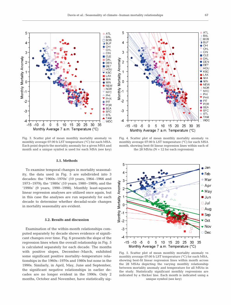
A plot of monthly mortality anomaly versus meanmonthly 07:00 h LST temperature exhibits a verystrong inverse relationship (Fig. 3). It is a characteristicof the US population that winter mortality greatlyexceeds summer mortality. The monthly variance ofwinter mortality is higher than in summer, partlybecause of the higher winter death rates and the possi-

65

SEA

POR

SFC

LAXPHX

DEN

MIN

KSC

CHI

STL CIN

DET

ATL

NEW

DAL

HOU

CHL

NORWDC

BALPITCLE

BUF BOSNYC

TAMMIA

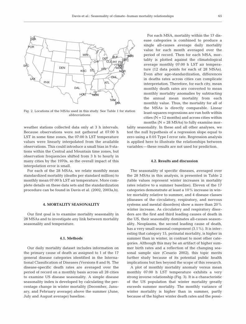
PHI

Fig. 2. Locations of the MSAs used in this study. See Table 1 for station abbreviations

Clim Res 26: 61–76, 2004

ble influence of cold-season diseases like influenza(see Section 6.2).

To investigate mortality seasonality at the MSAlevel, we examine the relationship between monthlyaverage 07:00 h LST temperature and the monthlyaverage mortality anomaly by calculating the best-fitlinear regression within each MSA (Fig. 4). Becausethe y-axis depicts mortality anomalies constructedindividually for each MSA, and since winter mortalityexceeds summer mortality, most cities have moremonths with negative than positive mortality anom-alies. The variability in the x-direction is purely a func-tion of climate. The slope for each MSA indicates themortality sensitivity of the population to changes intemperature over the course of the year. Cities with thesteepest negative slopes (such as San Francisco, LosAngeles, Miami) are cities with little seasonal temper-ature variation and thus an apparent greater mortalityresponse to month-to-month temperature differences.Cities with the shallowest negative slopes (such asMinneapolis, Chicago, Detroit) have large intrannualtemperature variations and a low mortality response tomonthly temperature differences. The remaining citiesfall in between these extremes.

Another way to examine mortality seasonality is tocompare mortality in different cities within a givenmonth (Fig. 5). Using the same dataset, the between-city regressions show the relationship between airtemperature and mortality for each month. The statis-tically significant positive slopes (increasing mortality

with increasing temperature) for January, February,and March indicate that winter-mortality rates aresignificantly higher in warm cities than in cold ones.Conversely, the significant negative slopes for May,June, September, October, and November suggestthat mortality rates in these months are lower inwarmer locales. This result implies that, in general,cities with warmer winters have a greater annualmortality amplitude than colder cities. However, thisresult must be viewed with caution, because they-axis contains mortality anomalies standardized foreach MSA by the annual mean. Thus, a city with ahigh winter-mortality anomaly must also have a largesummer-mortality anomaly and a large seasonal-mortality amplitude because of the standardizationprocedure.

5. TEMPORAL SEASONALITY CHANGES

An initial interpretation of Fig. 5 suggests that winterwarming results in higher mortality and spring andautumn warming result in lower death rates. But thatanalysis contains no temporal component. To properlyanalyze the potential impact of climate change, it isnecessary to consider whether the relationships de-picted in Fig. 5 are stable over time. Therefore, our sec-ond goal is to determine whether the monthly patternsof mortality–climate seasonality have changed at thedecadal scale.

66

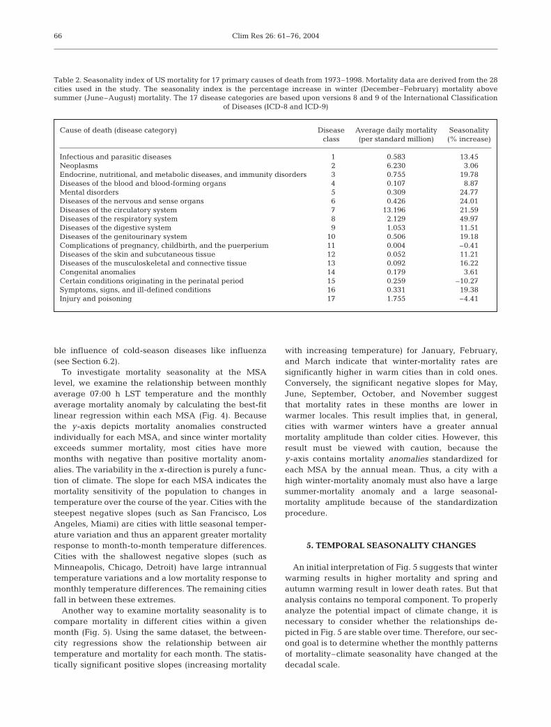
Cause of death (disease category) Disease Average daily mortality Seasonalityclass (per standard million) (% increase)

Infectious and parasitic diseases 1 0.583 13.45Neoplasms 2 6.230 3.06Endocrine, nutritional, and metabolic diseases, and immunity disorders 3 0.755 19.78Diseases of the blood and blood-forming organs 4 0.107 8.87Mental disorders 5 0.309 24.77Diseases of the nervous and sense organs 6 0.426 24.01Diseases of the circulatory system 7 13.1960 21.59Diseases of the respiratory system 8 2.129 49.97Diseases of the digestive system 9 1.053 11.51Diseases of the genitourinary system 10 0.506 19.18Complications of pregnancy, childbirth, and the puerperium 11 0.004 –0.41Diseases of the skin and subcutaneous tissue 12 0.052 11.21Diseases of the musculoskeletal and connective tissue 13 0.092 16.22Congenital anomalies 14 0.179 3.61Certain conditions originating in the perinatal period 15 0.259 –10.270Symptoms, signs, and ill-defined conditions 16 0.331 19.38Injury and poisoning 17 1.755 –4.41

Table 2. Seasonality index of US mortality for 17 primary causes of death from 1973–1998. Mortality data are derived from the 28cities used in the study. The seasonality index is the percentage increase in winter (December–February) mortality abovesummer (June–August) mortality. The 17 disease categories are based upon versions 8 and 9 of the International Classification

of Diseases (ICD-8 and ICD-9)


5.1. Methods

To examine temporal changes in mortality seasonal-ity, the data used in Fig. 5 are subdivided into 3decades: the ‘1960s–1970s’ (10 years; 1964–1966 and1973–1979); the ‘1980s’ (10 years; 1980–1989); and the‘1990s’ (9 years; 1990–1998). Monthly least-squareslinear regression analyses are utilized once again, butin this case the analyses are run separately for eachdecade to determine whether decadal-scale changesin mortality seasonality are evident.


Examination of the within-month relationships com-puted separately by decade shows evidence of signifi-cant changes over time. Fig. 6 presents the slope of theregression lines when the overall relationship in Fig. 5is calculated separately for each decade. The monthswith positive slopes, December–March, exhibitedsome significant positive mortality–temperature rela-tionships in the 1960s–1970s and 1980s but none in the1990s. Similarly, in April, May, June and September,the significant negative relationships in earlier de-cades are no longer evident in the 1990s. Only 2months, October and November, have statistically sig-

67

Fig. 3. Scatter plot of mean monthly mortality anomaly vsmonthly average 07:00 h LST temperature (°C) for each MSA.Each point depicts the mortality anomaly for a given MSA andmonth and a unique symbol is used for each MSA (see key)

Fig. 4. Scatter plot of mean monthly mortality anomaly vsmonthly average 07:00 h LST temperature (°C) for each MSAmonth, showing best-fit linear regression lines within each of

the 28 MSAs (N = 12 for each regression)

Fig. 5. Scatter plot of mean monthly mortality anomaly vsmonthly average 07:00 h LST temperature (°C) for each MSA,showing best-fit linear regression lines within month acrossthe 28 MSAs depicting the varying monthly relationshipbetween mortality anomaly and temperature for all MSAs inthe study. Statistically significant monthly regressions areindicated by a thicker line. Each month is indicated using a

unique symbol (see key)

Clim Res 26: 61–76, 2004

nificant mortality–temperature slopes in the 1990s.From the 1960s through the 1980s, MSAs with higheraverage December–March temperatures had greatermortality anomalies than MSAs with lower averagetemperatures. Conversely, from April–June and Sep-tember–November, warmer cities had comparablylower mortality. But almost all of these relationshipswere no longer apparent by the 1990s. Thus, over time,the strength of the relationship between monthly mor-tality anomalies and temperatures between US citieshas become muted.

Because few of the slopes differ in the 1990s, thisresult suggests that there are few intercity (or climate-related) differences in mortality seasonality across theUS—in other words, the average annual mortalitycycle, which is similar across US cities, is largely inde-pendent of climate. The overarching implication of thisresult indicates that there is no net mortality benefit toone’s place of residence derived from the location’sclimate. This finding is apparently contrary to the gen-eral perception within the populace that one’slongevity can be increased by moving to warmerlocales. (It is interesting that Laschewski & Jendritzky(2002) found that in Germany, on a weekly scale, tran-sitions toward cooler conditions within all seasonsresulted in lower mortality rates.) While there may beother longevity benefits to be derived from one’s loca-tion that are distinct from climate, the data for the1990s indicate little seasonal difference in mortalityrates between US cities.

This result also calls into question the approach thathas been used to determine climate-change impacts byidentifying ‘surrogate’ cities whose projected future

climates most resemble the contemporary climates ofsome cities (National Assessment Synthesis Team2000). For example, if in the future the climate of Char-lotte (North Carolina) is expected to become more likeAtlanta’s (Georgia) current climate, one might con-sider using the regression relationships from Atlanta toproject Charlotte’s future mortality seasonality for eachmonth. But this approach is problematic in several dif-ferent ways. First, it implies that the mortality responseto heat of the populace in surrogate cities is compara-ble to that of the base city. But differences in urbaninfrastructure, health care, housing types, etc., allimpact mortality rates (Smoyer 1993). Second, thismethod implicitly assumes that future weather–mortality relationships will be comparable to the aver-age, past relationships (i.e. that the time series of themortality response to weather is stationary). Our priorresearch demonstrates that this assumption is invalidin US cities (Davis et al. 2002, 2003a,b). Third, by the1990s, the monthly mortality–temperature relation-ships were almost identical in most MSAs.

Thus, there is little merit in the ‘surrogate city’approach to mortality forecasting.

6. IMPACTS OF CLIMATE CHANGE ONMORTALITY

Our third goal is to assess the impact of climatechange on observed patterns of mortality–climateseasonality and examine how potential future patternsof temperature change may influence future mortal-ity rates.

6.1. Methods

We wish to investigate the sensitivity of future mor-tality to patterns of potential temperature change.Thus far, our analyses have been based upon annu-ally normalized monthly mortality anomalies for eachcity. But these are not appropriate for projection pur-

68

Fig. 6. Slope of the best-fit least-squares regression line be-tween the average monthly mortality anomaly vs 07:00 h LSTtemperature (°C) across all 28 MSAs for each month and

decade. #Statistically significant regression slope

Fig. 7. Average daily total mortality, by decade, for the 28 MSAs examined in this study


poses because of the between-month linkage inherentin the standardization procedure used to computemortality anomalies (i.e. a large positive Januaryanomaly forces a large negative July anomaly). Toestimate future mortality, we must examine actualmortality counts (still standardized as rates per stan-dard million population) rather than anomalies(monthly departures). Thus, simple monthly average,age-standardized mortality counts are used in thisportion of the analysis.

There has been a systematic temporal decline inadjusted death rates across all cities that is (presum-ably) unrelated to climate (Fig. 7). Improved healthcare, technological advances, reducedpoverty, etc. (hereafter referred to as ‘tech-nological’ influences), have resulted ingreater average longevity in the US. Butthese declines have also taken place duringa period of background climate warming.For the 28 cities in this study over our1964–1998 period of record, 07:00 h LSTtemperatures have increased in all months,with the largest warming from January–March and May–August (Fig. 8). Some com-ponent of these temperature trends may berelated to increased greenhouse-gas con-centrations, but they also include urbaniza-tion effects that diurnally are most evident inmorning observations (e.g. Kalnay & Cai2003).

Because of advances in medical technol-ogy and other factors, mortality rates havedeclined over time across the US (Fig. 7)thereby complicating our analysis. Toremove this inherent ‘technological trend’from the monthly mortality data for eachMSA, the annual time series for each of the12 months is individually regressed againstthe annual total death rate (sum of 12monthly values), the results of which we useas an indicator of the overall technological

trend. Thus, the sample size for each of the 336 regres-sions (12 mo × 28 MSAs) is N = 29 yr. For all city-months, this relationship is highly statistically signifi-cant (p < 0.0001 for all but 1 case). Typical examplesare presented for the Kansas City MSA for Januaryand July, respectively (Fig. 9a,b).

The residuals from this regression analysis—monthly mortality departures from the technologicaltrend line—are then regressed against 07:00 h LSTtemperature (again, N = 29) for each month (Fig. 9c,d).This analysis also requires 336 regressions represent-ing the strength of the temperature signal in the mor-tality data for each month and city. Because of thesmall size of these samples and the higher probabilitythat the fundamental regression assumption of inde-pendent identically distributed residuals could easilybe violated, estimates of the regression slopes (betas)are bootstrapped (with replacement) 10 000 times anda new frequency distribution of beta is established.Based upon the 2.5 and 97.5 percentile observations inthe bootstrap sample, a determination is made for eachcase as to whether the mean regression slope signifi-cantly differs from zero. Any resulting significant rela-tionships between residual mortality and temperatureshould therefore be largely independent of technolog-ical influences that resulted in temporally decliningdeath rates.

69

Fig. 8. Mean trend (°C/decade) of 07:00 h LST temperature,by month, for the 28 MSAs in this study. Shaded bars indicatethose months with statistically significant regression slopes

(α ≤ 0.05)

Fig. 9. (a,b) Best-fit least-squares linear regression of (a) January and(b) July average mortality vs total annual mortality for the Kansas CityMSA. (c,d) Linear regressions of (c) January and (d) July residuals vs

07:00 h LST temperature (ºC) for the Kansas City MSA

Clim Res 26: 61–76, 2004

Now that monthly mortality–temperature relation-ships have been identified for each MSA and month,independent of technological trends, it is possible toestimate the past mortality change over our period ofrecord given the observed temperature trends and toproffer some insights on the potential impacts of futureclimate change. For each city-month with statisticallysignificant mortality–temperature relationships, theslope (mean beta value from the bootstrapped distrib-ution of betas) of the mortality–temperature regressionrelationship is multiplied by the observed temperaturechange, to produce a mortality change over the periodof record.

We also use the beta values for each statistically sig-nificant city-month to estimate future mortality rates(change in deaths per decade) by multiplying theregression slopes by several different seasonal temper-

ature change patterns. We apply 3 different tempera-ture change situations to each city to demonstrate thesensitivity of the results to the seasonal patterns ofpotential climate change: a uniform 1°C warmingacross all months; a winter-dominant warming (1.5°Cmo−1 from October–March and 0.5°C mo−1 fromApril–September); and a summer-dominant warming(1.5°C mo−1 in the warm half-year and 0.5°C mo−1 inthe cold half-year). The individual city responses arethen summed to produce a net national response. Ourgoal here is not to forecast future mortality rates but toexamine the sensitivity of mortality to a few differentinter-monthly patterns of temperature change. Thisallows us to examine the issue of how a winter warm-ing might compensate for increased summer mortalityduring hot months—a topic that lies at the heart of theseasonal mortality issue.

70

MSA Jan Feb Mar Apr May Jun Jul Aug Sep Oct Nov Dec Pos. Neg. Sig. Sig. pos. neg.

ATL –0.188 –0.205 –0.23 –0.286 –0.084 0.043 0.113 0.073 –0.201 –0.208 –0.092 –0.124 3 9 0 2BAL –0.056 0.232 –0.208 –0.298 –0.166 0.131 0.45 –0.215 0.046 –0.122 –0.038 –0.145 4 8 1 0BOS –0.007 0.28 –0.107 –0.227 –0.129 0.13 0.219 0.401 –0.157 –0.25 –0.26 –0.313 4 8 0 2BUF –0.324 0.209 0.06 0.007 –0.315 0.155 0.258 0.328 –0.1 0.063 –0.185 –0.189 7 5 0 2CHI –0.042 0.103 –0.123 –0.13 –0.037 0.06 0.467 0.063 0.061 –0.155 –0.098 –0.164 5 7 1 3CHL –0.214 –0.224 –0.342 –0.572 0.132 0.253 0.243 –0.199 –0.103 –0.263 –0.107 –0.067 3 9 0 2CIN –0.161 –0.049 –0.139 0.023 0.096 0.019 0.126 0.042 –0.054 –0.148 –0.143 –0.159 5 7 0 0CLE –0.106 0.019 –0.076 –0.063 –0.115 0.167 0.36 –0.0003 0.02 –0.051 –0.051 –0.186 4 8 0 1DAL –0.154 0.027 –0.012 –0.197 0.111 0.212 0.581 0.321 –0.111 –0.018 –0.163 0.197 6 6 2 0DEN –0.047 0.021 0.206 –0.165 0.001 –0.088 0.079 –0.058 0.118 –0.124 0.035 0.291 8 4 1 0DET –0.104 0.055 0.043 –0.109 0.085 0.175 0.448 0.181 –0.047 –0.084 –0.206 –0.111 6 6 3 1HOU –0.179 –0.18 –0.142 –0.087 0.085 0.071 0.288 0.541 0.105 –0.113 –0.196 –0.3 5 7 1 2KSC –0.107 –0.1 –0.024 –0.369 –0.107 –0.151 0.717 –0.142 –0.089 –0.126 –0.093 –0.051 2 100 0 1LAX –0.323 –0.41 0.071 –0.166 –0.108 0.037 0.037 0.243 0.117 –0.065 –0.292 0.04 6 6 1 1MIA –0.279 –0.203 0.25 –0.086 –0.042 0.246 –0.047 –0.106 0.234 0.035 –0.036 –0.229 4 8 0 0MIN –0.019 0.051 –0.108 –0.203 –0.036 –0.013 0.163 0.156 –0.118 –0.151 –0.028 –0.022 4 8 0 0NEW –0.350 –0.362 –0.124 –0.454 0.184 0.075 0.513 0.375 –0.205 –0.367 –0.360 –0.407 4 8 0 5NOR –0.215 0.147 –0.41 –0.08 0.289 –0.071 0.073 –0.086 –0.058 –0.128 –0.251 –0.254 3 9 0 0NYC –0.030 0.091 –0.122 –0.194 0.007 0.211 0.814 0.291 –0.075 –0.142 –0.141 –0.158 5 7 1 1PHI –0.135 0.11 –0.166 –0.01 –0.144 0.046 0.468 0.138 –0.026 –0.17 –0.212 –0.274 4 8 1 2PHX –0.095 –0.154 0.163 –0.078 –0.282 –0.038 0.026 –0.075 0.038 0.03 –0.056 0.337 5 7 0 0PIT –0.207 0.004 0.121 –0.461 –0.1 0.064 0.236 –0.044 0.012 –0.133 –0.116 –0.154 5 7 0 1POR –0.197 –0.56 –0.012 –0.309 –0.074 0.096 0.367 0.597 –0.055 0.109 –0.094 –0.17 5 7 1 2SEA –0.151 –0.482 –0.473 –0.21 –0.047 0.127 0.063 0.339 0.115 –0.013 0.053 –0.26 5 7 1 2SFC –0.386 –0.523 –0.249 –0.345 –0.079 –0.286 –0.008 0.059 –0.011 0.057 –0.146 –0.253 2 100 0 2STL –0.072 –0.06 –0.098 –0.173 0.011 –0.036 1.52 0.01 –0.043 –0.062 –0.075 –0.064 3 9 1 0TAM –0.213 –0.309 –0.096 –0.131 0.085 0.227 0.052 0.126 –0.047 –0.089 –0.224 –0.195 4 8 0 3WDC –0.086 0.261 –0.111 –0.059 0.09 –0.149 0.341 –0.005 0.044 –0.133 –0.092 –0.054 4 8 1 1

Positive 4 14 7 2 12 20 26 18 11 5 2 4 125Negative 24 14 21 26 16 8 2 10 17 23 26 24 211Sig. pos. 0 0 0 0 0 1 8 6 0 0 0 1 16Sig. neg. 2 3 0 7 1 0 0 0 0 8 8 7 36

Table 3. Beta values (slopes) of the regressions for mortality (with the technological trend removed) vs 07:00 h LST temperaturefor each MSA and month. Regression slopes are the means of the distribution of 10 000 bootstrapped samples of beta for each MSA-month. Statistically significant slopes (2.5 and 97.5% confidence intervals) are calculated using the percentile method and indicated in bold. Marginals include counts of the number of significant and total positive and negative relationships in

each column



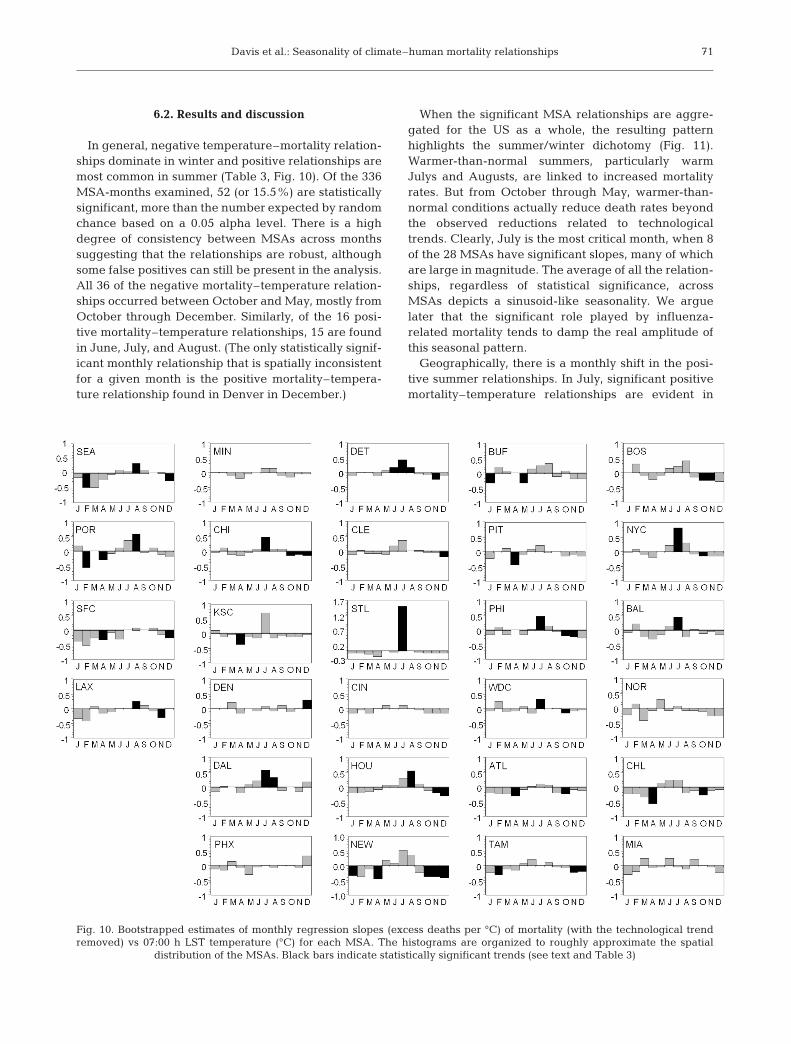
In general, negative temperature–mortality relation-ships dominate in winter and positive relationships aremost common in summer (Table 3, Fig. 10). Of the 336MSA-months examined, 52 (or 15.5%) are statisticallysignificant, more than the number expected by randomchance based on a 0.05 alpha level. There is a highdegree of consistency between MSAs across monthssuggesting that the relationships are robust, althoughsome false positives can still be present in the analysis.All 36 of the negative mortality–temperature relation-ships occurred between October and May, mostly fromOctober through December. Similarly, of the 16 posi-tive mortality–temperature relationships, 15 are foundin June, July, and August. (The only statistically signif-icant monthly relationship that is spatially inconsistentfor a given month is the positive mortality–tempera-ture relationship found in Denver in December.)

When the significant MSA relationships are aggre-gated for the US as a whole, the resulting patternhighlights the summer/winter dichotomy (Fig. 11).Warmer-than-normal summers, particularly warmJulys and Augusts, are linked to increased mortalityrates. But from October through May, warmer-than-normal conditions actually reduce death rates beyondthe observed reductions related to technologicaltrends. Clearly, July is the most critical month, when 8of the 28 MSAs have significant slopes, many of whichare large in magnitude. The average of all the relation-ships, regardless of statistical significance, acrossMSAs depicts a sinusoid-like seasonality. We arguelater that the significant role played by influenza-related mortality tends to damp the real amplitude ofthis seasonal pattern.

Geographically, there is a monthly shift in the posi-tive summer relationships. In July, significant positivemortality–temperature relationships are evident in

71

Fig. 10. Bootstrapped estimates of monthly regression slopes (excess deaths per °C) of mortality (with the technological trendremoved) vs 07:00 h LST temperature (°C) for each MSA. The histograms are organized to roughly approximate the spatial

distribution of the MSAs. Black bars indicate statistically significant trends (see text and Table 3)

Clim Res 26: 61–76, 2004

New York, Philadelphia, Baltimore, Washington, DC,Detroit, Chicago, St. Louis, and Dallas (Fig. 10). Withthe exception of Dallas, all of these cities are in thenortheast-north central US. Although hot and humidsummer weather is not uncommon in these regions,prior research has demonstrated that cities in thenortheastern quadrant of the continental US are mostsusceptible to summer heat mortality (Kalkstein &Davis 1989, Davis et al. 2003a,b). In August, of the 6cities with significant positive relationships—Detroit,Houston, Dallas, Los Angeles, Portland, and Seattle—5 are located in Texas or along the West Coast. Thisgeographic shift suggests that the nexus of summerhigh temperature mortality impacts can vary withinseason. The peak mortality in West Coast cities couldbe related to an increased prevalence of Santa Anawinds and their associated high temperatures. It islikewise possible that August heat events in the north-east and northern interior have a reduced impactbecause of ‘mortality displacement’—the July heathad already resulted in excess mortality (Kalkstein &Smoyer 1993, Kalkstein & Greene 1997, Laschewski &Jendritzky 2002). However, July is typically warmerthan August in the southern and western MSAs as wellas in the Northeast, so mortality displacement alonecannot explain this monthly geographical shift.

Interpretation is more complicated in the cold season.Winter mortality is believed to be higher because of theenhanced spread of infectious diseases as people spendmore time in closer proximity, thereby increasing theinfection rate (Eurowinter Group 1997). Indeed, infec-

tious disease mortality is higher in winter(Table 2). Influenza and pneumonia account forover 5000 excess deaths yr−1 (Simonsen et al.2001) and are largely responsible for the sea-sonality in the mortality from respiratory dis-eases (Table 2). However, influenza infectioncan result in deaths attributed to other causes,and these co-morbid factors may account forthe observed seasonality in some other diseasecategories (Simonsen et al. 2001). Thus, part ofthe winter peak is directly attributable to in-fluenza, part is related to co-morbid conditions,and part is probably unrelated to influenza inany way but simply reflects some other in-herent seasonal fluctuation.

Although influenza is a winter disease,efforts to relate the strength of the flu virus orinfluenza-related mortality to weather and cli-mate have been largely unsuccessful. It is notthe case that severe winters have higher ratesof influenza infections or mortality (Frost &Auliciems 1993). However, influenza mortalitydoes vary substantially from year to year(Simonsen et al. 2001), for reasons that, at pre-

sent, remain unknown. Recent studies have found thatinfluenza-related mortality rates have been increasingover time in the US (Thompson et al. 2003).

Given the lack of a relationship between climate andinfluenza, the temporal trend in influenza deaths, andthe impact of influenza on diseases in other cause-of-death categories, it is difficult to fully understand therelationships between climate and mortality in wintermonths. In most cities, there is a strong tendency forthe relationship to be negative—warm winters areassociated with fewer deaths than cold winters. Thistendency becomes most pronounced starting in Octo-ber and continues through April, with the exception ofFebruary, which exhibits many positive and negativerelationships (Table 3). In reality, the primary influenzaseason begins in late fall and has typically ended byMarch or April, if not sooner (Simonsen et al. 2001). Ifthe influence of influenza is to mask mortality–temperature relationships, then we might look to Aprilas an indicator of the correct magnitude of this interac-tion. Using April–October as guidance, superpositionof a curve on the seasonal course of climate-relatedmortality suggests that we are probably significantlyunderestimating the impact of climate on cold-seasonmortality (Fig. 11). However, this is mere speculation,and it may ultimately prove very difficult to effectivelyremove the influenza signal from the backgroundseasonal mortality pattern in the historical time series.Obviously, there is no simple cause–effect relation-ship between winter mortality and the thermal envi-ronment.

72

Fig. 11. Monthly average mortality–temperature relationship for the28 study MSAs. Black histogram bars represent the average of the sta-tistically significant relationships only (non-significant slopes are set tozero prior to calculating the mean). Grey histogram bars show themean of all slopes regardless of significance. The superimposed curveis a hypothesized mortality–temperature seasonality relationshipestimated using the months when influenza is uncommon (see text in

Section 6.2)


One might argue that influenza deaths be removedfrom the analysis a priori. Some mortality researcherschose to work specifically with diseases known tobe weather-related and discard all others (e.g.Sakamoto-Momiyama 1977, Auliciems & Skinner1989, Seretakis et al. 1997, McGregor 1999, 2001,McGregor et al. 2004). However, significant relation-ships remain evident using all-causes mortality (e.g.Applegate et al. 1981, Kalkstein & Davis 1989, Kunstet al. 1993). To date, however, it has been difficult toisolate the influence of influenza and co-morbid con-ditions from the mortality signal, so simple removal ofdeaths directly attributable to influenza will notaddress this problem. Even though we are knowinglyincluding deaths that are not likely to be relatedto weather and climate, our approach is conserv-ative, since this biases our analysis toward notfinding significant relationships.

The observed pattern of temperature change,with a net warming of 1.16°C since 1964 andsome warming in all months (Fig. 8), results inthe excess summer deaths being partiallycancelled by the reduction in winter death rates(Fig. 12). Although most of the warming hasoccurred from January–March, these wintermonths exhibit only very weak negative temper-ature–mortality relationships. Thus, the warmingin July and August, though somewhat less thanwhat occurred in winter, has a greater net mor-tality impact. The net impact of the observedtemperature change over our period of record isan increase of 2.9 deaths in the annual total mor-tality (per standard million) per city since 1964—a number that is very small relative to the annual

death rate of about 9500 deaths (per stan-dard million) during the 1990s. If these pro-jections are within an order of magnitude ofthe correct value, our results indicate thatthe observed, historical climate warminghas had very little influence on human mor-tality rates.

Future mortality projections indicate thatthe monthly pattern of temperature changewill be important in estimating future cli-mate-related death rates. Using 3 simplemonthly patterns of temperature seasonal-ity, we find that a uniform 1°C warmingresults in a net mortality decline of 2.65deaths (per standard million) per MSA, thesummer-dominant warming generates 3.61additional deaths, and the winter-dominantwarming produces 8.92 fewer deaths(Fig. 13). Again, these numbers are verysmall compared with the annual averagemortality rate.

It is important to reiterate that our analysis was per-formed at a coarse monthly scale because of the lack ofany strong daily relationships between mortality andweather in winter. Our goal was to examine the gen-eral seasonality of climate and mortality. A modeldeveloped to predict the number of excess deaths aris-ing from longer or more intense heat waves, for exam-ple, might produce different mortality estimates.Clearly, there remains a net impact of heat on mortal-ity in the US, even after removal of the long-term tech-nological trend. However, on an annual basis, theinfluences of mortality displacement, mortality bene-fits from warmer winters, and technology tend to miti-gate against summer heat mortality. This analysis, in

73

Fig. 12. Number of excess or reduced deaths, by month, at the end of therecord compared with the beginning based on the observed monthlytemperature trend and the statistically significant mortality–temperaturerelationships (Fig. 10). The relationships are derived separately for each MSA-month and then combined to produce the 28-city national average

Fig. 13. Number of excess or reduced monthly deaths (MSA−1) under2 different climate-change scenarios, with 75% of the total annual

warming in the 6 coldest months and the 6 warmest months

Clim Res 26: 61–76, 2004

which we relate mean monthly temperatures (ratherthan weather events) to mortality, tends to smooth overthe impacts of specific events like heat waves and pro-vides a general idea of the linkages between a warm-ing climate and mortality patterns.

7. CONCLUSIONS AND IMPLICATIONS

Temperature currently does not have a major influ-ence on monthly mortality rates in US cities. By the1990s, there was little evidence of a net mortality ben-efit to be derived from one’s place of residence. In alllocations, warmer months have significantly lowermortality rates than colder months, undoubtedlyrelated to the impact of influenza during the cold sea-son, although influenza (and co-morbid influences)alone cannot account for the observed seasonality inmortality. The winter–summer mortality rate differ-ence of residents in Phoenix or Los Angeles, for exam-ple, is similar to those of people in Minneapolis orBoston. This consistency across cites with largely dif-ferent climate regimes can be partially attributed toadaptations (both biophysical and infrastructural) andinfluences of technology. The implication is that theseasonal mortality pattern in US cities is largely inde-pendent of the climate and thus insensitive to climatefluctuations, including changes related to increasinggreenhouse gases.

Our analysis of the relationship between monthlymortality and monthly temperature after taking intoaccount the technological influences on declining mor-tality rates represents one of the first efforts of its kindto assess the net impact of seasonal climate variabilityon mortality, although admittedly in a somewhat rudi-mentary manner. We find that the lives saved in con-junction with warm winters do tend to offset the addi-tional deaths associated with warmer conditions inJuly and August. However, again we stress that theindividual MSA plots of monthly mortality–tempera-ture relationships (Fig. 10) provide more evidence thatclimate impacts on US mortality are very small. Wefind that the net impact of the observed temperaturechange from 1964 to 1998 is far less than 0.1% of theaverage total annual mortality in the 1990s. Thisimplies that impacts of a future climate change that arewithin 1 or even 2 orders of magnitude of those ob-served during the past 35 yr will be very small.

Our finding of small net future mortality impactsfrom increasing temperatures, and of positive mortal-ity–temperature relationships in summer and negativerelationships in winter, are in general agreement withresearch conducted in other industrialized nations. Forexample, Guest et al. (1999) noted that future mortalityimpacts in Australia’s 5 largest cities would be small by

2030. McGregor et al. (2004) found that years withstrong temperature seasonality also exhibited elevatedmortality from ischaemic heart disease in 5 Englishcounties. In research conducted for Germany, Lerchl(1998) emphasized the importance of extreme cold rel-ative to extreme heat in association with high mortalityrates, although extremes also generated higher overallmortality, as in our research. But Laschewski & Jen-dritzky’s (2002) work in southwest Germany noted thatsummer heat wave mortality exceeded that associatedwith cold conditions in winter.

Perhaps the primary impact of our research will be toemphasize how little is known about the seasonality ofmortality and its relationship to climate. Before we canbegin to make confident projections of future impacts,much additional work is needed on this topic. Animportant component of this seasonality is the roleplayed by climate on influenza transmission, becauseinfluenza has a major influence on higher winter-mortality rates. The general lack of clear relationshipsbetween winter weather and mortality on a daily basissuggests that cold-weather events do not significantlyraise mortality rates. However, in aggregate, ourresults indicate that cold winters do have higher netmortality than warm winters, for reasons that, at leastat present, remain unknown.

Acknowledgements. We extend our thanks to Laurence S.Kalkstein, Daniel Graybeal, and Jill Derby Watts (Universityof Delaware) for providing the raw mortality data used in thisstudy and for their assistance in reading the digital data sets.We also extend our heartfelt thanks to 3 anonymous review-ers, who provided exceptionally detailed and thoughtfulreviews of our original submission. It is becoming increas-ingly rare for referees to provide this level of critique, and weappreciate their interest in our manuscript.

LITERATURE CITED

Anderson RN, Rosenberg HM (1998) Age standardization ofdeath rates: implementation of the year 2000 standard.National Vital Statistics Reports 47(3), National Center forHealth Statistics, Hyattsville, MD

Applegate WB, Runyan JW Jr, Brasfield L, Williams MLM,Konigsberg C, Fouche C (1981) Analysis of the 1980 heatwave in Memphis. J Am Geriatr Soc 29:337–342

Auliciems A, Skinner JL (1989) Cardio-vascular deaths andtemperature in subtropical Brisbane. Int J Biometeorol 33:215–221

Bentham CG (1997) Health. In: Palutikof JP, Subak S, AgnewMD (eds) Economic impacts of the hot summer and unusu-ally warm year of 1995. Department of the Environment,Washington, DC, p 87–95

Bluestein M, Zecher J (1999) A new approach to an accuratewind chill factor. Bull Am Meteorol Soc 80:1893–1900

Bridger CA, Ellis FP, Taylor HL (1976) Mortality in St. Louis,Missouri, during heat waves in 1936, 1953, 1954, 1955 and1966. Environ Res 12:38–48

Cesario SK (2002) The ‘Christmas Effect’ and other biometeo-

74


rologic influences on childbearing and the health ofwomen. J Obstetr Gynecol Neonatal Nurs 31:526–535

Changnon SA, Kunkel KE, Reinke BC (1996) Impacts andresponses to the 1995 heat wave: a call to action. Bull AmMeteorol Soc 77:1496–1506

Danet S, Richard F, Montaye M, Beauchant S and 5 others(1999) Unhealthy effects of atmospheric temperature andpressure on the occurrence of myocardial infarction andcoronary deaths. A 10-year survey: the Lille-World HealthOrganization MONICA project (Monitoring trends anddeterminants in cardiovascular disease). Circulation100:E1–E7

Davis RE, Knappenberger PC, Novicoff WM, Michaels PJ(2002) Decadal changes in heat-related human mortalityin the Eastern US. Clim Res 22:175–184

Davis RE, Knappenberger PC, Novicoff WM, Michaels PJ(2003a) Decadal changes in summer mortality in U.S.cities. Int J Biometeorol 47:166–175

Davis RE, Knappenberger PC, Michaels PJ, Novicoff WM(2003b) Changing heat-related mortality in the UnitedStates. Environ Health Perspect 111:1712–1718

Donaldson GC, Keatinge WR (1997) Early increases inischaemic heart disease mortality dissociated from andlater changes associated with respiratory mortality aftercold weather in south east England. J Epidemiol CommHealth 51:643–648

Donaldson GC, Ermakov SP, Komarov YM, McDonald CP,Keatinge WR (1998) Cold related mortalities and protec-tion against cold in Yakutsk, eastern Siberia: observationand interview study. Br Med J 317:978–982

Eng H, Mercer JB (1998) Seasonal variations in mortalitycaused by cardiovascular diseases in Norway and Ireland.J Cardiovascular Risk 5:89–95

Eurowinter Group (1997) Cold exposure and winter mortalityfrom ischaemic heart disease, cerebrovascular disease,respiratory disease, and all causes in warm and coldregions of Europe. Lancet 349:1341–1346

Frost DB, Auliciems A (1993) Myocardial infarct death, thepopulation at risk, and temperature habituation. Int J Bio-meteorol 37:46–51

Glass R, Zack M (1979) Increase in deaths from ischemic heartdisease after blizzards. Lancet 3:485–487

Gorjanc ML, Flanders WD, VanDerslice J, Hersh J, Malilay J(1999) Effects of temperature and snowfall on mortality inPennsylvania. Am J Epidemiol 149:1152–1160

Gover M (1938) Mortality during periods of excessive temper-ature. Public Health Rep 53:1122–1143

Guest CS, Willson K, Woodward AJ, Hennessy K, KalksteinLS, Skinner C, McMichael AJ (1999) Climate and mortalityin Australia: retrospective study, 1979–1990, and predictedimpacts in five major cities in 2030. Clim Res 13:1–15

Hayden BP (1998) Ecosystem feedbacks on climate at thelandscape scale. Phil Trans R Soc Lond Ser B 352:5–18

IPCC (2001a) Climate change 2001: impacts, adaptation, andvulnerability. Contribution of Working Group II. In:McCarthy JJ, Osvaldo FC, Leary NA, Dokken DJ, WhiteKS (eds) Third Assessment Report of the Intergovernmen-tal Panel on Climate Change. Cambridge University Press,Cambridge

IPCC (2001b) Climate change 2001: the scientific basis. Con-tribution of Working Group I. In: Houghton JT, Ding Y,Griggs DJ, Noguer M, van der Linden PJ, Dai X, MaskellK, Johnson CA (eds) Third Assessment Report of theIntergovernmental Panel on Climate Change. CambridgeUniversity Press, Cambridge

Kalkstein LS (1993) Health and climate change—directimpacts in cities. Lancet 342:1397–1399

Kalkstein LS, Davis RE (1989) Weather and human mortality:an evaluation of demographic and interregional responsesin the United States. Ann Assoc Am Geogr 79:44–64

Kalkstein LS, Greene JS (1997) An evaluation of climate/mor-tality relationships in large U.S. cities and the possibleimpacts of a climate change. Environ Health Perspect 105:84–93

Kalkstein LS, Smoyer KE (1993) The impact of climate changeon human health: some international implications. Experi-entia 49:969–979

Kalnay E, Cai M (2003) Impact of urbanization and land-usechange on climate. Nature 423:528–531

Kilbourne EM (1997) Heat waves and hot environments. In:Noji EK (ed) The public health consequences of disaster.Oxford University Press, New York, p 245–269

Kloner RA, Poole WK, Perritt RL (1999) When throughout theyear is coronary death most likely to occur? A 12-yearpopulation-based analysis of more than 220,000 cases.Circulation 100:1630–1634

Kunst AE, Looman CWN, Mackenbach JP (1993) Outdoor airtemperature and mortality in the Netherlands: a timeseries analysis. Am J Epidemiol 137:331–341

Langford IH, Bentham G (1995) The potential effects of cli-mate change on winter mortality in England and Wales.Int J Biometeorol 38:141–147

Lanska DJ, Hoffmann RG (1999) Seasonal variation in strokemortality rates. Neurology 52:984−990

Larsen U (1990a) The effects of monthly temperature fluctua-tions on mortality in the United States from 1921 to 1985.Int J Biometeorol 34:136–145

Larsen U (1990b) Short-term fluctuations in death by cause,temperature, and income in the United States 1930–1985.Soc Biol 37:172–187

Laschewski G, Jendritzky G (2002) Effects of the thermalenvironment on human health: an investigation of 30years of daily mortality data from SW Germany. Clim Res21:91–103

Lerchl A (1998) Changes in the seasonality of mortality inGermany from 1946 to 1995: the role of temperature. IntJ Biometeorol 42:84–88

Lyster WR (1976) Death in summer [letter]. Lancet 2:469Marmor M (1975) Heat wave mortality in New York City,

1949 to 1970. Arch Environ Health 30:130–136McGregor GR (1999) Winter ischaemic heart disease deaths

in Birmingham, UK: a synoptic climatological analysis.Clim Res 13:17–31

McGregor GR (2001) The meteorological sensitivity ofischaemic heart disease mortality events in Birmingham,UK. Int J Biometeorol 45:133–142

McGregor GR, Watkin HA, Cox M (2004) Relationshipsbetween the seasonality of temperature and ischaemicheart disease mortality: implications for climate basedhealth forecasting. Clim Res 25:253–263

Michaels PJ, Balling Jr RC (2000) The satanic gases: clearingthe air about global warming. Cato Institute, Washington,DC

Michaels PJ, Balling Jr RC, Vose RS, Knappenberger PC(1998) Analysis of trends in the variability of daily andmonthly historical temperature measurements. Clim Res10:27–33

Moore TG (1998) The health and amenity benefits of globalwarming. Econ Inquiry July:471–488

National Assessment Synthesis Team (2000) Climate changeimpacts on the United States: the potential consequencesof climate variability and change. US Global ChangeResearch Program, Washington, DC

National Center for Health Statistics (1998) Compressed mor-

75

Clim Res 26: 61–76, 2004

tality file. US Dept Health Human Service, Public HealthService, CDC, Atlanta, GA

National Climatic Data Center (1993) Solar and meteorologi-cal surface observation network 1961–1990. NationalClimatic Data Center, Asheville, NC

National Climatic Data Center (1997) Hourly United Statesweather observations 1990–1995. National Climatic DataCenter, Asheville, NC

National Environmental Satellite, Data, and Information Ser-vice (2000) TD-3280 US Surface Airways and AirwaysSolar Radiation Hourly. US Department of Commerce,Washington, DC

Oechsli FW, Buechley RW (1970) Excess mortality associatedwith three Los Angeles September hot spells. Environ Res3:277–284

Osczevski RJ (1995) The basis of wind chill. Arctic 48:372–382

Pell JP, Cobbe SM (1999) Seasonal variations in coronaryheart disease. Q J Med 92:689–696

Quayle RG, Steadman RG (1998) The Steadman wind chill: animprovement over present scales. Weather Forecast 13:1187–1193

Sakamoto-Momiyama M (1977) Seasonality in human mortal-ity. University of Tokyo Press, Tokyo

Schuman SH (1972) Patterns of urban heat-wave deaths andimplications for prevention: data from New York and St.Louis during July, 1966. Environ Res 5:59–75

Schuman SH, Anderson CP, Oliver JT (1964) Epidemiology ofsuccessive heat waves in Michigan in 1962 and 1963. J AmMed Assoc 180:131–136

Seretakis D, Lagiou P, Lipworth L, Signorello LB, RothmanKJ, Trichopoulos D (1997) Changing seasonality of mortal-ity from coronary heart disease. J Am Med Assoc 278:1012–1014

Simonsen L, Clarke MJ, Williamson GD, Stroup DF, ArdenNH, Schonberger LB (2001) The impact of influenza epi-demics on mortality: introducing a severity index. Am JPub Health 87:1944–1950

Smoyer KE (1993) Socio-demographic implications in summerweather-related mortality. MA thesis, University ofDelaware, Newark

Smoyer KE, Rainham GC, Hewko JN (2000) Heat-stress-related mortality in five cities in Southern Ontario:1980–1996. Int J Biometeorol 44:190–197

Steadman RG (1971) Indices of wind chill of clothed persons.J Appl Meteorol 10:674–683

Thompson WM, Shay DK, Weintraub E, Brammer L, Cox N,Anderson LJ, Fukuda K (2003) Mortality associated withinfluenza and respiratory syncytial virus in the UnitedStates. J Am Med Assoc 289:179–186

United States Department of Commerce (1973, 1982, 1992,2001) General population characteristics, United States.US Department of Commerce, Bureau of the Census,Washington, DC

76

Editorial responsibility: Andrew Comrie,Tucson, Arizona, USA

Submitted: June 26, 2003; Accepted: February 23, 2004Proofs received from author(s): April 2, 2004

Documents

Seasonality of climate–human mortality relationships in US ... · Seasonality of climate–human mortality relationships in US cities and impacts of climate ... tionships between