Embed Size (px)
Citation preview

Sec.3 Practical application
临床处方剂量的计算

What we should calculate?
Time or mu required to delivery proper dose for tumor
Dose distribution at the region of tumor
What kind of Parameters we should consider in dose
calculation?
Field size and shape
Depth
Beam quality
Calibration of output : SSD technique or SAD technique:
Radiotherapy institution vary in their treatment techniques and
calibration practices.

处方剂量 (prescription dose)
为达到一定的靶区(或肿瘤)剂量( DT)所需要的使用射野的射野中心轴上最大剂量点处的剂量,即处方剂量 Dm。
Rember :prescription dose is not air dose

The main contents
Accelerator calculations1. SSD technique
2. Isocentric technique
Cobalt-60 calculations Irregular fields Other practical methods of calculating
depth dose distribution

SSD technique Percent depth dose is a suitable quantity for calculations
involving SSD techniques.
Machines are usually calibrated to deliver 1rad(10-2Gy) per monitor unit(MU) at the reference field size 10×10cm and a source-to-calibration point distance of SCD.
Assuming that the Sc factors relate to collimator field sizes
defined at the SAD, the monitor units necessary to deliver a certain tumor dose(TD) at depth d for a field size r at the surface at any SSD are given by the following.

SSD technique
SSDfactorrSrSPDD
TDMU
pcC

SSD technique

SSD technique
2
0
tSSD
SCDSSDfactor
SSD
SADrrc
Where rc is the collimator field size, given by
It must be remembered that, whereas the field size for the SC factor is defined at the SAD, the Sp factors relate to the field irradiating the patient.

Example 1. A 4-MV linear accelerator is calibrated to give
1rad per MU in phantom at a reference depth of
maximum dose of 1cm, 100cmSSD, and
10×10cm field size. Determine the MU values to
deliver 200rads(cGy) to a patient at 100cm
SSD, 10cm depth, and 15×15cm field size,
given SC(15×15)=1.020, Sp(15×15)=1.010,
PDD(10,15×15,100)=65.1%

Answer:
2981010.1020.1651.0
200
SSDfactorSSPDD
DTMU
PC

Example 2. Determine the MU for the treatment conditions
given in Example 1 except that the treatment SSD is 120cm, given SC(12.5×12.5)
=1.010 Answer:
697.01120
1100
5.12120
10015(100cm) SADat projected size Field
2
SSDfactor
442697.0010.1010.1667.0
200
MU

Isocentric technique TMR is the quantity of choice for dosimetric calculations involving
isocentric techniques.
Since the unit is calibrated to give 1rad/MU at the reference depth t0,
calibration distance SCD and for the reference field (10cm×10cm),
then the monitor units necessary to deliver isocentric dose (ID) at
depth d are give by the following:
2
factor
,
SAD
SCDSAD
SADfactorrSrSrdTMR
IDMU
dpcCd

Example 3. A tumor dose of 200 rads is to be delivered at the isocentric which
is located at a depth of 8cm, given 4-MV x-ray beam, field size at
the isocentric=6×6cm, Sc(6×6)=0.970, Sp(6×6)=0.990, machine
calibrated at SCD=100cm, TMR(8,6×6)=0.787. Since the
calibration point is at the SAD, SAD factor=1.
Answer:
2651990.0970.0787.0
200
MU

Example 4. Calculate MU values for the case in Example 3, if the unit is
calibrated nonisocentrically, i.e. source to calibration point
distance=101cm.
Answer:
26002.199.0970.0787.0
200
020.1100
1012
MU
SADfactor

Cobalt-60 calculation The above calculation system is sufficiently general that it can be
applied to any radiation generator including 60Co.
In the latter case, the machine can be calibrated either in air or in phantom provided the following information is available:1. Dose rateD0(t0,r0,f0) in phantom at depth t0 of maximum dose for a reference field r0 and standard SSD f0; 2. Sc factor; 3. Sp factor; 4.PDD and TMR values.
If universal depth dose data for 60Co are used, then the Sp factor and TMR can be obtained by using the following equations:
d
d
d
p
rBSF
rdTARrdTMR
rBSF
rBSFrS
,,
0

Example 5. A tumor dose of 200 rads is to be delivered at 8cm depth,
using 15×15cm field size, 100cm SSD, and penumbra
trimmers up. The unit is calibrated to give 130rads/min in
phantom at 0.5cm depth for a 10×10cm field with trimmers up
and SSD=80cm. Determine the time of irradiation, given
SC(12×12)=1.012, Sp(15 ×15)=1.014, PDD(8,
15×15,100)=68.7%.

Answer: field size projected at SAD (80cm)
min40.3642.0014.1012.1687.0130
200
15151212100,1515,880,1010,5.0
642.05.0100
5.080
1212100
8015
2
SSDfactorSSPDDD
TDTIME
SSDfactor
cmcm
pC

Dose calculation in irregular fields--- Clarkson’s method
Any field other than the rectangular, square, or circular field may be
termed irregular.
Irregularly shaped fields are encountered in radiotherapy when
radiation sensitive structures are shielded from the primary beam or
when the field extends beyond the irregularly shaped patient body
contour.
Examples of such fields are the mantle and inverted Y fields employed
for the treatment of Hodgkin’s disease.

Dose calculation in irregular fields--- Clarkson’s method
Since the basic data are available usually for rectangular fields,
methods are required to use these data for general cases of irregularly
shape fields. One such method, originally proposed by Clarkson and
later developed by Cunningham, has proved to be the most general in
its application.
Clarkson’s method is based on the principle that the scattered
component of the depth dose, which depends on the field size and
shape, can be calculated separately from the primary component
which is independent of the field size and shape. A special
quantity,SAR, is used to calculate the scattered dose.


Dose calculation in irregular fields--- Clarkson’s method
Assume this field cross section to be at depth d and perpendicular to the beam axis. Let Q be the point of calculation in the plane of the field cross section.
Radii are drawn from Q to divide the field into elementary sectors. Each sector is characterized by its radius and can be considered as part of a circular field of that radius.
If we suppose the sector angle is 10º, then the scatter contribution from this sector will be 10º/360º=1/36 of that contributed by a circular field of that radius and centered at Q.

Dose calculation in irregular fields--- Clarkson’s method
Thus, the scatter contribution from all the sectors can be calculated and summated by considering each sector to be a part of its own circle whose scatter-air ratio is already known and tabulated.
Using an SAR table for circular fields, the SAR values for the sectors are calculated and then summed to give the average SAR for the irregular field at point Q.
For sectors passing through a blocked area,the net SAR is determined by subtracting the scatter contribution by the blocked part of sector.

Dose calculation in irregular fields--- Clarkson’s method
For example,
The computed average SAR is converted to average TAR by the equation:
QBQCQA
BCQAQC
SARSARSAR
SARSARSAR
net
SARTARTAR 0

Dose calculation in irregular fields--- Clarkson’s method
BSF can be calculated by Clarkson’s method. This involves determining average TAR at the depth dm on the axis, using the field contour or radii projected at the depth dm.
BSFdf
dfTARPDD
eTAR
m
dd m
1
02

Other practical methods
Irregular fields Point off-axis Point outside the field Point under the block

Irregular fields Clarkson’s techniques is a general method of
calculating depth dose distribution in an irregularly shaped field but it is not practical for routine manual calculations.
Even when computerized, it is time consuming since a considerable amount of input data is required by the computer program.
However, with the exception of mantle, inverted Y, and a few other complex fields, reasonably accurate calculations can be made for most blocked fields using an approximate method .

Irregular fields Approximate rectangles may be drawn containing the point
of calculation so as to include most of the irradiated area surrounding the point and exclude only those areas that are remote to the point.
In so doing, a blocked area may be included in the rectangle provided this area is small and is remotely located relative to that point.
The rectangle thus formed may be called the effective field while the unblocked field, defined by the collimator, may be called collimator field.
It is important to remember that, whereas the SC factors are relatedto the collimator field, the PDD,TMR, or SP
corresponds to the effective field.


Point off-axis
It is possible to calculate depth dose distributions at any point within the field or outside the field using Clarkson’s technique. However, it is not practical for manual calculations.
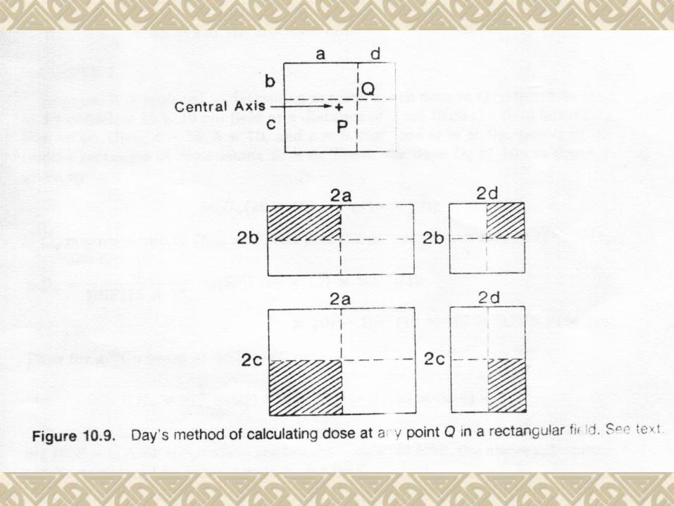
Day has proposed a particularly simple calculation method for rectangular fields. In this method, PDD can be calculated at any point within the medium using the central axis data.
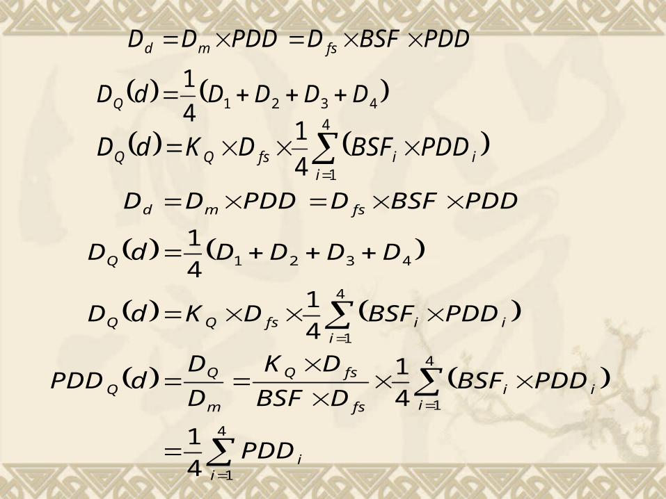
43214
1DDDDdD
PDDBSFDPDDDD
Q
fsmd
4
1
4
1
4
1
4321
4
1
4
1
4
14
1
ii
iii
fs
fsQ
m
iiifsQQ
Q
fsmd
PDD
PDDBSFDBSF
DK
D
DdPDD
PDDBSFDKdD
DDDDdD
PDDBSFDPDDDD
4
14
1
iiifsQQ PDDBSFDKdD

4321
4
1
4
1i
4
1
4
1
4
1
PDDPDDPDDPDDPDD
PDD
PDDBSFDBSF
DK
D
DdPDD
Q
ii
iifs
fsQ
m

Suppose the field size is 15×15cm. a=10, b=5, c=10,d=5, assume KQ=0.98
and SSD=80cm. PDDP=58.4%
PDDQ=55.8%
KQ=1,PDDQ=56.9%
This off-axis decrease in dose is due to the reduced scatter at Q
compared to P. Similarly, it can be shown that the magnitude of the
reduction in scatter depends on the distance of Q from P as well as
depth.

Point outside the field

中大
中中大大
中大
PDDPDDPDD
baBSF
PDDBSFPDDBSFPDD
DDD
Q
Q
Q
2
1
2
2
1

Suppose
it is required to determine PDD at Q (relative to Dm
at P) outside a 15×10cm field at a distance of 5cm
from the field border. a=15, b=10,c=5. Suppose Q is
at the center of the middle rectangle of dimensions
2c×b. Then the dose DQ at 10cm depth is given by
the above equation.
PDDQ=2.1%

Think about :
Point outside field
Point under block


![[XLS] · Web viewSheet1 流水号 通用名 剂型 小剂型 规格 包装 剂型详细 剂型说明 包装详细 包材说明 质量层次 生产企业 投标企业 醋酸钙 冲剂](https://img.pdfslide.net/doc/110x75/5af0fdb97f8b9ac2468eca9f/xls-viewsheet1-.jpg)