(Second Best) Alternatives to Randomized Designs

(Second Best) Alternatives to Randomized Designs

Mark W. LipseyPeabody Research Institute, Vanderbilt University

IES/NCER Summer Research Training Institute, 2010

Quasi-Experimental Designs to Discuss

Regression discontinuity Nonrandomized comparison groups with

statistical controls Analysis of covariance Matching Propensity scores

The Regression-Discontinuity (R-D) Design

Advantages of the R-D design?

When well-executed, its internal validity is strong– comparable to a randomized experiment.

It is adaptable to many circumstances where it may be difficult to apply a randomized design.

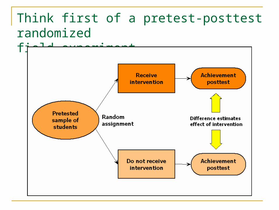
Think first of a pretest-posttest randomized field experiment

Posttest on pretest regression for randomized experiment (with no treatment effect)

Pretest (S)

Posttest (Y)

Mean S

T

C

iiTiSi eTBSBBY 0

Corresponding regression equation (T: 1=treatment, 0=control)

Mean Y

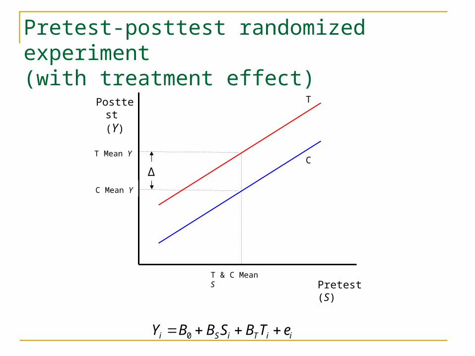
Pretest-posttest randomized experiment(with treatment effect)

Pretest (S)

Posttest (Y)

T & C Mean S

T

C

iiTiSi eTBSBBY 0

C Mean Y

T Mean Y

Δ

Regression discontinuity(with no treatment effect)

Selection Variable (S)

Posttest (Y)

Cutting Point

T

C

iiTiSi eTBSBBY 0

C Mean Y

T Mean Y

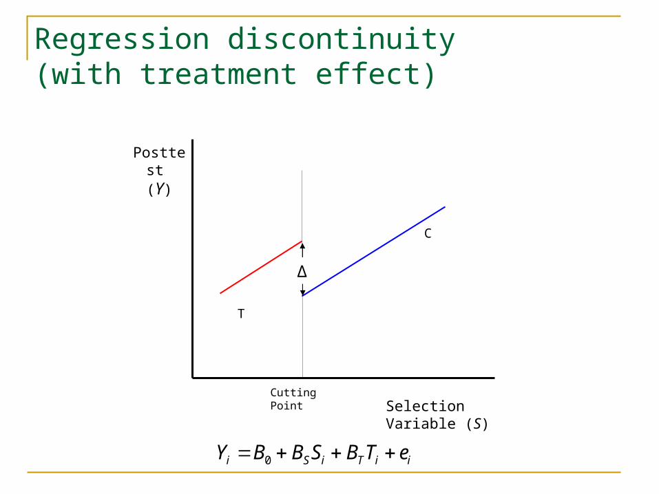
Regression discontinuity(with treatment effect)


Posttest (Y)

Cutting Point

T

C

iiTiSi eTBSBBY 0

Δ

Regression discontinuity effect estimate compared with RCT estimate


Posttest (Y)

T

C

iiTiSi eTBSBBY 0

Δ

Cutting Point

Regression discontinuity scatterplot (null case)


Posttest (Y)

Cutting Point

TC

iiTiSi eTBSBBY 0

Regression discontinuity scatterplot (Tx effect)


Posttest (Y)

Cutting Point

T

C

iiTiSi eTBSBBY 0

The selection variable for R-D

A continuous quantitative variable measured on every candidate for assignment to T or C who will participate in the study

Assignment to T or C strictly on the basis of the score obtained and a predetermined cutting point

Does not have to correlate highly with the outcome variable (more power if it does)

Can be tailored to represent an appropriate basis for the assignment decision in the setting

Why does it work?

There is selection bias and nonequivalence between the T and C groups but …

its source is perfectly specified by the cutting point variable and can be statistically modeled (think perfect propensity score)

Any difference between the T and C groups that might affect the outcome, whether known or unknown, has to be correlated with the cutting point variable and be “controlled” by it to the extent that it is related to the outcome (think perfect covariate)

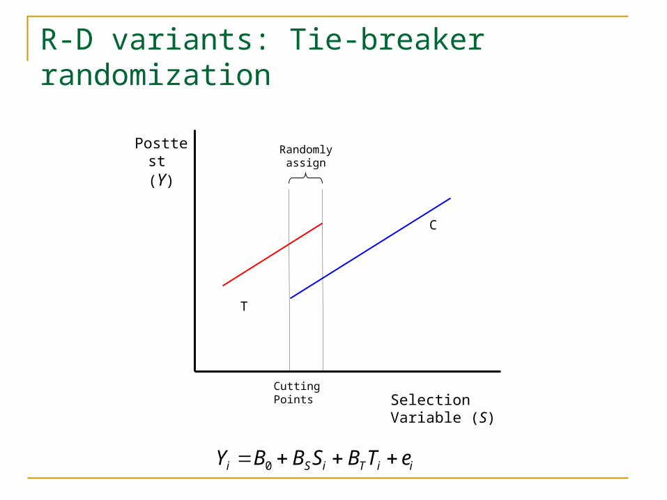
R-D variants: Tie-breaker randomization


Posttest (Y)

Cutting Points

T

C

iiTiSi eTBSBBY 0

Randomlyassign

R-D variants: Double cutting points


Posttest (Y)

Cutting Points

T1

C

iiTiTiSi eTBTBSBBY 22110

T2

Special issues with the R-D design

Correctly fitting the functional form– possibility that it is not linear curvilinear functions interaction with the cutting point consider short, dense regression lines

Statistical power sample size requirements relative to RCT when covariates are helpful

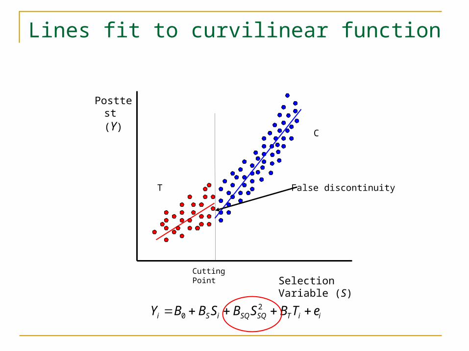
Lines fit to curvilinear function


Posttest (Y)

Cutting Point

T

C

False discontinuity

iiTSQSQiSi eTBSBSBBY 20

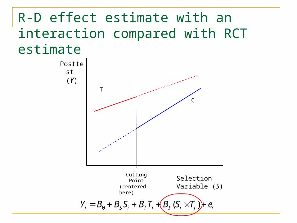
R-D effect estimate with an interaction compared with RCT estimate


Posttest (Y)

T

C

iiiIiTiSi eTSBTBSBBY )(0

Cutting Point(centered here)

Modeling the functional form

Visual inspection of scatterplots with candidate functions superimposed is important

If possible, establish the functional form on data observed prior to implementation of treatment, e.g., pretest and posttest archival data for a prior school year

Reverse stepwise modeling– fit higher order functions and successively drop those that are not needed

Use regression diagnostics– R2 and goodness of fit indicators, distribution of residuals

Short dense regressions for R-D


Posttest (Y)

Cutting Point

T

C

iiTiSi eTBSBBY 0

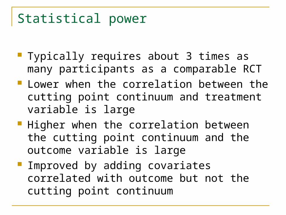
Statistical power

Typically requires about 3 times as many participants as a comparable RCT

Lower when the correlation between the cutting point continuum and treatment variable is large

Higher when the correlation between the cutting point continuum and the outcome variable is large

Improved by adding covariates correlated with outcome but not the cutting point continuum

Example: Effects of pre-k

W. T. Gormley, T. Gayer, D. Phillips, & B. Dawson (2005). The effects of universal pre-k on cognitive development. Developmental Psychology, 41(6), 872-884.

Study overview

Universal pre-k for four year old children in Oklahoma

Eligibility for pre-k determined strictly on the basis of age– cutoff by birthday

Overall sample of 1,567 children just beginning pre-k plus 1,461 children just beginning kindergarten who had been in pre-k the previous year

WJ Letter-Word, Spelling, and Applied Problems as outcome variables

Samples and testing

pre-k kindergarten

pre-k

First cohort

Second cohort

Year 1 Year 2

AdministerWJ tests

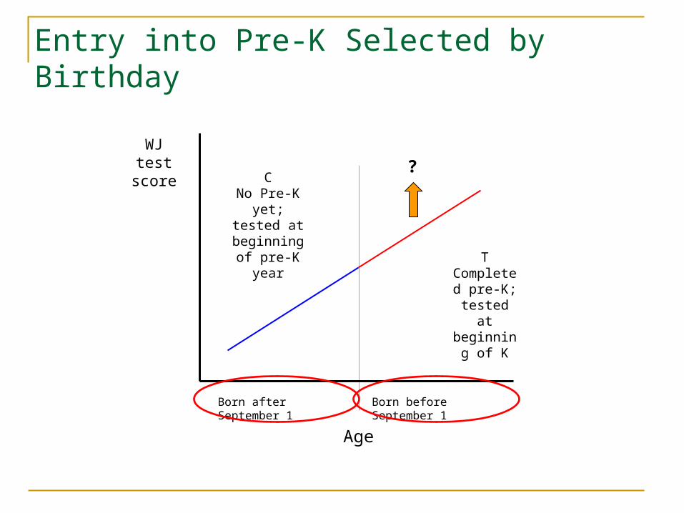
Entry into Pre-K Selected by Birthday

WJ testscore

Born before September 1

T Completed

pre-K; tested at beginning

of K

Born after September 1

Age

CNo Pre-K

yet; tested at beginning of pre-K year

?

Excerpts from Regression Analysis

Letter-Word Spelling Applied Probs

Variable B coeff B coeff B coeff

Treatment (T) 3.00* 1.86* 1.94*

Age: Days ± from Sept 1 .01 .01* .02*

Days2 .00 .00 .00

Days x T .00 -.01 -.01

Days2 x T .00 .00 .00

Free lunch -1.28* -.89* -1.38*

Black .04 -.44* -2.34*

Hispanic -1.70* -.48* -3.66*

Female .92* 1.05* .76*

Mother’s educ: HS .59* .57* 1.25* * p<.05

Selected references on R-D

Shadish, W., Cook, T., and Campbell, D. (2002). Experimental and quasi-experimental designs for generalized causal inference. Boston: Houghton Mifflin.

Mohr, L.B. (1988). Impact analysis for program evaluation. Chicago: Dorsey. Hahn, J., Todd, P. and Van der Klaauw, W. (2002). Identification and estimation

of treatment effects with a regression-discontinuity design. Econometrica, 69(1), 201-209.

Cappelleri J.C. and Trochim W. (2000). Cutoff designs. In Chow, Shein-Chung (Ed.) Encyclopedia of Biopharmaceutical Statistics, 149-156. NY: Marcel Dekker.

Cappelleri, J., Darlington, R.B. and Trochim, W. (1994). Power analysis of cutoff-based randomized clinical trials. Evaluation Review, 18, 141-152.

Jacob, B. A. & Lefgren, L. (2002). Remedial education and student achievement: A regression-discontinuity analysis. Working Paper 8919, National Bureau of Economic Research (www.nber.org/papers/w8919)

Kane, T. J. (2003). A quasi-experimental estimate of the impact of financial aid on college-going. Working Paper 9703, National Bureau of Economic Research (www.nber.org/papers/w9703)

Nonrandomized Comparison Groups with Statistical Controls

ANCOVA/OLS statistical controls Matching Propensity scores

Nonequivalent comparison analog to the completely randomized design

Individuals are selected into treatment and control conditions through some nonrandom more-or-less natural process

Treatment Comparison

Individual 1 Individual 1


… …

Individual n Individual n

Nonequivalent comparison analog to the randomized block design

Block 1 … Block m

Treatment

Individual 1

…

…

Individual 1

… …

Individual n Individual n

Comparison

Individual n +1 Individual n+1

… …

Individual 2n Individual 2n

The nonequivalent comparison analog to the hierarchical design

Treatment Comparison

Cluster 1 Cluster m Cluster m+1 Cluster 2m

Individual 1

…


…

Individual 1

Individual 2 Individual 2 Individual 2 Individual 2

… … … …

Individual n Individual n Individual n Individual n

Issues for obtaining good Tx effect estimates from nonrandomized comparison groups The fundamental problem: selection bias Knowing/measuring the variables necessary and

sufficient to statistically control the selection bias characteristics on which the groups differ that are related

to the outcome relevant characteristics not highly correlated with other

characteristics already accounted for Using an analysis model that properly adjusts for

the selection bias, given appropriate control variables

Nonrandomized comparisons of possible interest

Nonequivalent comparison/control group for estimating treatment effects

Attrition analysis– comparing leavers and stayers, adjusting for differential attrition

Treatment on the treated analysis (TOT)– estimating treatment effects on those who actually received treatment.

Nonequivalent comparison groups: Pretest/covariate and posttest means

Pretest/Covariate(s) (X)

Posttest (Y)

T

C

iiTiXi eTBXBBY 0

Diff inpost

means

Diff inpretest/cov

means

Nonequivalent comparison groups: Covariate-adjusted treatment effect estimate


Posttest (Y)

T

C

iiTiXi eTBXBBY 0

Δ

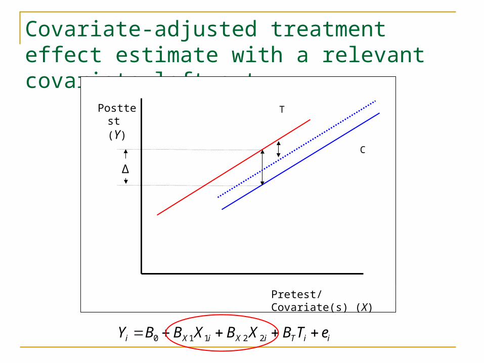
Covariate-adjusted treatment effect estimate with a relevant covariate left out


Posttest (Y)

T

C

iiTiXiXi eTBXBXBBY 22110

Δ

Nonequivalent comparison groups: Unreliability in the covariate


Posttest (Y)

Nonequivalent comparison groups: Unreliability in the covariate


Posttest (Y) T

C

iiTiXi eTBXBBY 0

Note: Will not always under- estimate, may over-estimate

Using control variables via matching

Groupwise matching: select control comparison to be groupwise similar to treatment group, e.g., schools with similar demographics, geography, etc. Generally a good idea.

Individual matching: select individuals from the potential control pool that match treatment individuals on one or more observed characteristics.May not be a good idea.

Potential problems with individual level matching

Basic problem with nonequivalent designs– need to match on all relevant variables to obtain a good treatment effect estimate.

If match on too few variables, may omit some that are important to control.

If try to match on too many variables, the sample will be restricted to the cases that can be matched; may be overly narrow.

If must select disproportionately from one tail of the treatment distribution and the other tail of the control distribution, may have regression to the mean artifact.

Regression to the mean: Matching on the pretest

T C

Area where matches can be found

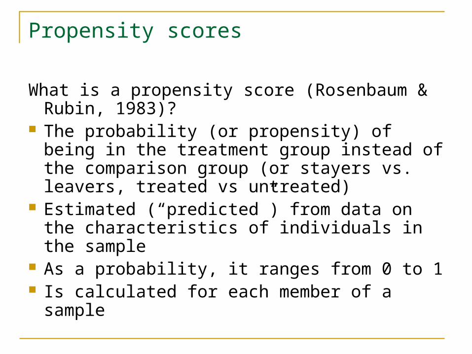
Propensity scores

What is a propensity score (Rosenbaum & Rubin, 1983)?

The probability (or propensity) of being in the treatment group instead of the comparison group (or stayers vs. leavers, treated vs untreated)

Estimated (“predicted”) from data on the characteristics of individuals in the sample

As a probability, it ranges from 0 to 1 Is calculated for each member of a sample

Computing the propensity score First estimate Ti = f(S1i, S2i, S3i … Ski) for all T and C

members in the sample Logistic regression typically used; other methods include

probit regression, classification trees All relevant characteristics assumed to be included among

the predictor variables (covariates) E.g., fit logistic regression Ti = B1S1i + B2S2i …+ ei Compute propensityi = B1S1i + B2S2i … Ski

The propensity score thus combines all the information from the covariates into a single variable optimized to distinguish the characteristics of the T sample from those of the C sample

What to do with the propensity score

Determine how similar the treatment and control group are on the composite of variables in the propensity score; decide if one or both need to be trimmed to create a better overall match.

Use the propensity score to select T and C cases that match.

Use the propensity score as a statistical control variable, e.g., in an ANCOVA.

Propensity score distribution before trimming (example from Hill pre-K Study)

0.0

5.1

.15

0.0

5.1

.15

0 1

0

1

Fra

ctio

n

propensity scoreGraphs by prek

Comparison Group (n=1,144):

25th percentile: 0.3050th percentile: 0.4075th percentile: 0.53Mean = 0.39

Treatment Group (n=908): 25th percentile: 0.4250th percentile: 0.5275th percentile: 0.60Mean = 0.50

Propensity score distribution after trimming (example from Hill pre-K Study)

0.0

5.1

.15

0.0

5.1

.15

0 1

0

1

Fra

ctio

n

propensity scoreGraphs by prek

Treatment Group (n=908): 25th percentile: 0.4250th percentile: 0.5275th percentile: 0.60Mean = 0.50

Comparison Group (n=908):25th percentile: 0.3650th percentile: 0.4575th percentile: 0.56Mean = 0.46

Estimate the treatment effect, e.g., by differences between matched strata

Propensity Score Quintiles

TreatmentGroup

ControlGroup

Matches

Estimate the treatment effect, e.g., by using the propensity score as a covariate

Propensity score (P)

Posttest (Y) T

C

iiTiPi eTBPBBY 0

Δ

Discouraging evidence about the validity of treatment effect estimates

The relatively few studies with head-to-head comparisons of nonequivalent comparison groups with statistical controls and randomized controls show very uneven results– some cases where treatment effects are comparable, many where they are not.

Failure to include all the relevant covariates appears to be the main problem.

Selected references on nonequivalent comparison designs

Rosenbaum, P.R., & Rubin, D.B. (1983). The central role of the propensity score in observational studies for causal effects. Biometrika 70(1): 41-55.

Luellen, J. K., Shadish, W.R., & Clark, M.H. (2005). Propensity scores: An introduction and experimental test. Evaluation Review 29(6): 530-558.

Schochet, P.Z., & Burghardt, J. (2007). Using propensity scoring to estimate program-related subgroup impacts in experimental program evaluations. Evaluation Review 31(2): 95-120.

Bloom, H.S., Michalopoulos, C., & Hill, C.J. (2005). Using experiments to assess nonexperimental comparison-group methods for measuring program effects. Chapter 5 in H. S. Bloom (ed.) Learning more from social experiments: Evolving analytic approaches (NY: Russell Sage Foundation), pp. 173-235.

Agodini, R. & Dynarski, M. (2004). Are experiments the only option? A look at dropout prevention programs. The Review of Economics and Statistics 86(1): 180-194.

Wilde, E. T & Hollister, R (2002). How close Is close enough? Testing nonexperimental estimates of impact against experimental estimates of impact with education test scores as outcomes,” Institute for Research on Poverty Discussion paper, no. 1242-02; http://www.ssc.wisc.edu/irp/.

Glazerman, S., Levy, D.M., & Myers, D. (2003). Nonexperimental versus experimental estimates of earnings impacts. Annals AAPSS, 589: 63-93.

Arceneaux, K., Gerber, A.S., & Green, D. P. (2006). Comparing experimental and matching methods using a large-scale voter mobilization experiment. Political Analysis, 14: 37-62.

Documents

(Second Best) Alternatives to Randomized Designs