Embed Size (px)
Citation preview

Second graded Second graded Homework Assignment:Homework Assignment:
1.80; 1.84; 1.92; 1.110; 1.115; 1.141
(optional: 1.127)
Due in Labs on Sept 14-15

Last Time:Last Time:

Two Formulae for Variance!
22
1
1XX
ns iDefinitional Formula:
2
1
1
1
2
1
1 n
iin
n
ii XX
nComputational
Formula:

Comment about “Variance”• The concept and definition of variance that
we have so far talked about in class is often referred to as
Sample Variance• We will later discuss a different concept,
definition (and different formula) for what is commonly referred to as
Population VarianceThe latter is a theoretical variance, not a data variance.

a
b
InterceptSlope
bx+a
x
Reminder: (Simple) Linear Function y=a+bx

1 2 3 4 5 6 7 8 9 10
X
1 2 3 4 5 6 7 8 9 10
X+5
If we add the constant a=5to each observation,then we obtain newdata that are shifted by 5
A shift affects the meanbut not the variance
New mean = Old mean + 5
New variance = Old variance

1 2 3 4 5 6 7 8 9 10
X
1 2 3 4 5 6 7 8 9 10
2X
If we multiply each observation by the constant b=2, then we obtain a new data set that looks rather different
A multiplicative constant affects both the mean
and the variance
New mean = Old mean x 2
New variance = Old variance x 4
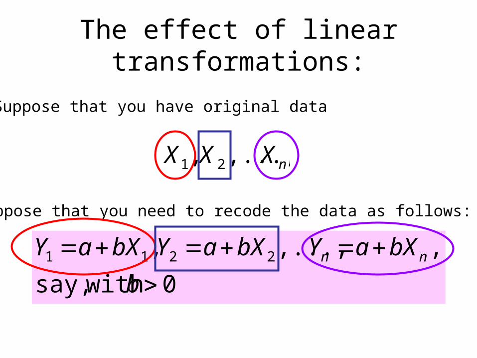
The effect of linear transformations:
Suppose that you have original data
nXXX ,...,, 21
Suppose that you need to recode the data as follows:
0 with say,
,,...,, 2211
b
bXaYbXaYbXaY nn
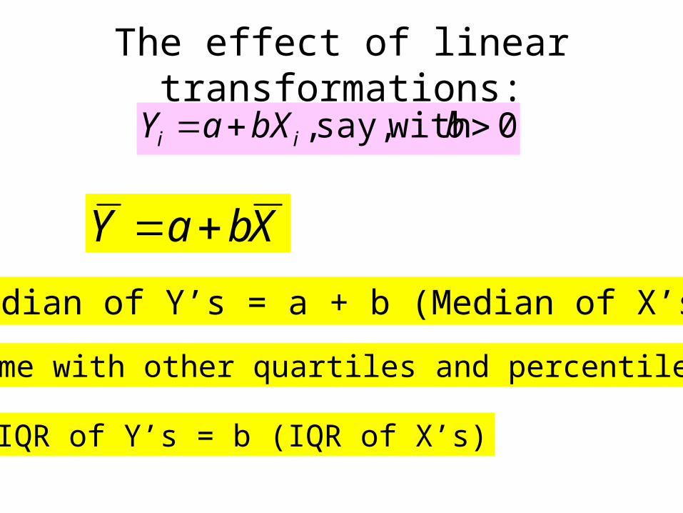
The effect of linear transformations:
0 with say,, bbXaY ii
XbaY
Median of Y’s = a + b (Median of X’s)
Same with other quartiles and percentiles
IQR of Y’s = b (IQR of X’s)

The effect of linear transformations:
0 with say,, bbXaY ii
222XY sbs
XY bss
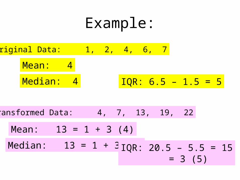
Example:
Original Data: 1, 2, 4, 6, 7
Transformed Data: 4, 7, 13, 19, 22
Mean: 4
Mean: 13 = 1 + 3 (4)
Median: 4
Median: 13 = 1 + 3 (4)
IQR: 6.5 – 1.5 = 5
IQR: 20.5 – 5.5 = 15= 3 (5)

Example:Original Data: 1, 2, 4, 6, 7
Transformed Data: 4, 7, 13, 19, 22
Variance:
Variance:
22222
41 4746444241
5.694049 426
41
22222
41 132213191313137134
5.58813603681 4234
41 5.63 2
Y = 1 + 3 X

0Z 12 Zs 1Zs
Transformation to Z-scores:
X
iiss
Xi s
XXXZ
XX
1
Z-scores have Mean equal to zero and (Variance) Standard Deviation equal to one

Today:Today:
The Normal DistributionThe Normal Distribution
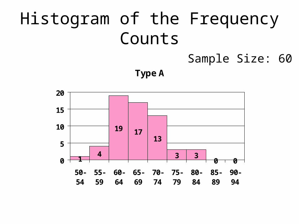
Histogram of the Frequency Counts
Type A
14
19 1713
3 30 00
5
10
15
20
50-54
55-59
60-64
65-69
70-74
75-79
80-84
85-89
90-94
Sample Size: 60

Type A
00.050.1
0.150.2
0.250.3
0.35
50-54
55-59
60-64
65-69
70-74
75-79
80-84
85-89
90-94
Histogram of the Proportions

Type A
50-54
55-59
60-64
65-69
70-74
75-79
80-84
85-89
90-94
Ca
libra
te a
pp
rop
riat
ely
Choose vertical unit such that the total orange area is equal to 1

Type A
50-54
55-59
60-64
65-69
70-74
75-79
80-84
85-89
90-94
Ca
libra
te a
pp
rop
riat
ely
Choose Vertical Unit such that the total orange area is equal to 1
3/6019/60

Type A
50-54
55-59
60-64
65-69
70-74
75-79
80-84
85-89
90-94
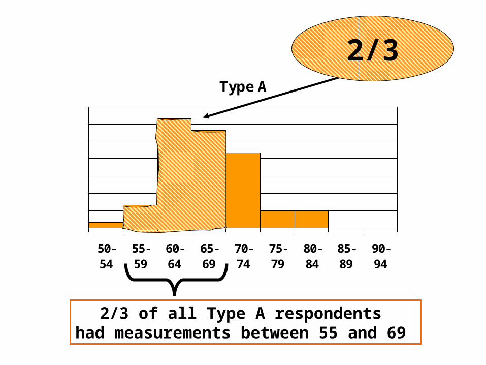
(4+19+17)/60
Type A
50-54
55-59
60-64
65-69
70-74
75-79
80-84
85-89
90-94
2/3
2/3 of all Type A respondents had measurements between 55 and 69

50-54
55-59
60-64
65-69
70-74
75-79
80-84
85-89
90-94
50-54
55-59
60-64
65-69
70-74
75-79
80-84
85-89
90-94
DataWorld
TheoryWorld

50-54
55-59
60-64
65-69
70-74
75-79
80-84
85-89
90-94
Density Function
It can be mathematically easier to work with such a curve instead of a histogram

Density Function
The marked area is the relative frequencywith which observations between a and b occur
ba
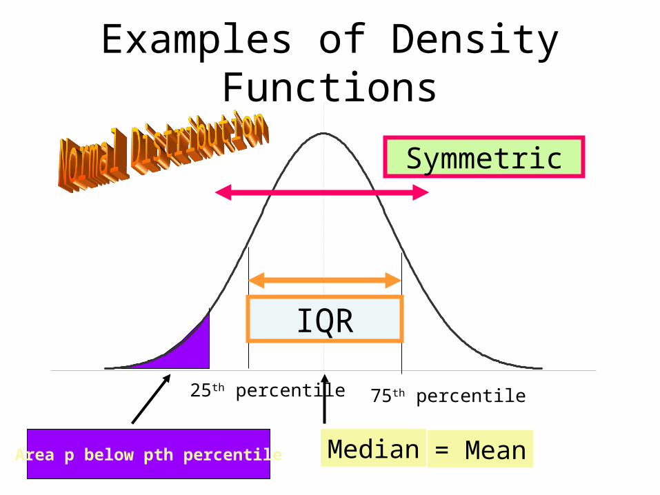
Examples of Density Functions
Median
75th percentile25th percentile
Area p below pth percentile
Symmetric
= Mean
IQR

Examples of Density Functions
Median Mean
Positively Skewed (Skewed to the right)

Examples of Density Functions
MedianMean
Negatively Skewed (Skewed to the left)

THE NORMAL DISTRIBUTIONTHE NORMAL DISTRIBUTION(“Gaussian”, “bell-shaped”)
Probably the single most important distribution in Statistics
Symmetric

THE NORMAL DISTRIBUTIONTHE NORMAL DISTRIBUTION
Notation: X ~ N( , )
A normal distribution is fully specified with just two ‘parameters’, the mean of the distribution () and the standard deviation of the distribution ().
DataWorld
TheoryWorld
ssX ,, 2
,, 2 No formulae
yet
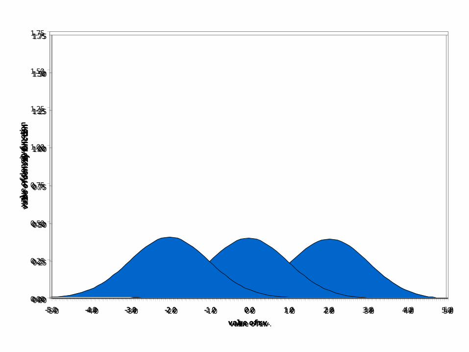
0.00
0.25
0.50
0.75
1.00
1.25
1.50
1.75
-5.0 -4.0 -3.0 -2.0 -1.0 0.0 1.0 2.0 3.0 4.0 5.0
value of r.v.
val
ue
of
de
nsi
ty f
un
ctio
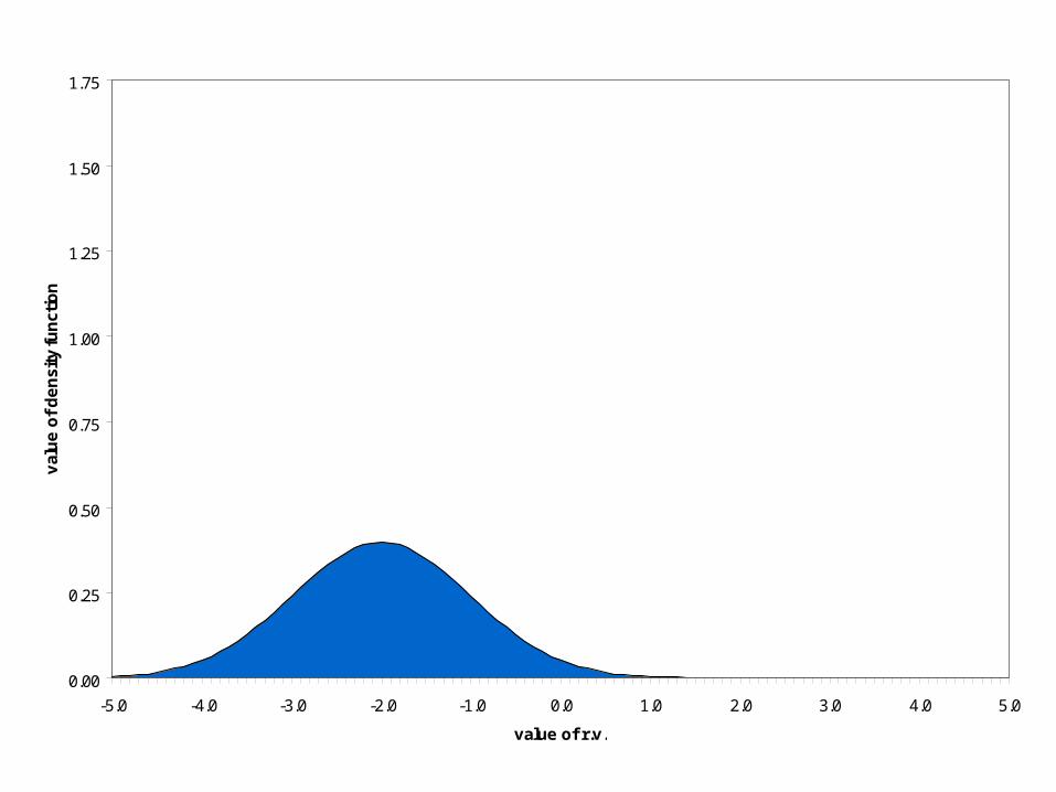
nN( -2 , 1 )
0.00
0.25
0.50
0.75
1.00
1.25
1.50
1.75
-5.0 -4.0 -3.0 -2.0 -1.0 0.0 1.0 2.0 3.0 4.0 5.0
value of r.v.
val
ue
of
de
nsi
ty f
un
ctio
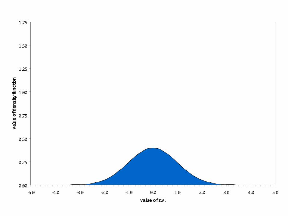
nN( 0 , 1 )

0.00
0.25
0.50
0.75
1.00
1.25
1.50
1.75
-5.0 -4.0 -3.0 -2.0 -1.0 0.0 1.0 2.0 3.0 4.0 5.0
value of r.v.
val
ue
of
de
nsi
ty f
un
ctio
nN( 2 , 1 )
0.00
0.25
0.50
0.75
1.00
1.25
1.50
1.75
-5.0 -4.0 -3.0 -2.0 -1.0 0.0 1.0 2.0 3.0 4.0 5.0
value of r.v.
val
ue
of
de
nsi
ty f
un
ctio
nN( 2 , 1 )
0.00
0.25
0.50
0.75
1.00
1.25
1.50
1.75
-5.0 -4.0 -3.0 -2.0 -1.0 0.0 1.0 2.0 3.0 4.0 5.0
value of r.v.
val
ue
of
de
nsi
ty f
un
ctio
nN( 0 , 1 )
0.00
0.25
0.50
0.75
1.00
1.25
1.50
1.75
-5.0 -4.0 -3.0 -2.0 -1.0 0.0 1.0 2.0 3.0 4.0 5.0
value of r.v.
val
ue
of
de
nsi
ty f
un
ctio
n
N( -2 , 1 )

0.00
0.25
0.50
0.75
1.00
1.25
1.50
1.75
-5.0 -4.0 -3.0 -2.0 -1.0 0.0 1.0 2.0 3.0 4.0 5.0
value of r.v.
va
lue
of
de
ns
ity
fu
nc
tio
n

0.00
0.25
0.50
0.75
1.00
1.25
1.50
1.75
-5.0 -4.0 -3.0 -2.0 -1.0 0.0 1.0 2.0 3.0 4.0 5.0
value of r.v.
val
ue
of
de
nsi
ty f
un
ctio
nN( 0 , 1 )

0.00
0.25
0.50
0.75
1.00
1.25
1.50
1.75
-5.0 -4.0 -3.0 -2.0 -1.0 0.0 1.0 2.0 3.0 4.0 5.0
value of r.v.
va
lue
of
de
ns
ity
fu
nc
tio
n

0.00
0.25
0.50
0.75
1.00
1.25
1.50
1.75
-5.0 -4.0 -3.0 -2.0 -1.0 0.0 1.0 2.0 3.0 4.0 5.0
value of r.v.
va
lue
of
de
ns
ity
fu
nc
tio
n
0.00
0.25
0.50
0.75
1.00
1.25
1.50
1.75
-5.0 -4.0 -3.0 -2.0 -1.0 0.0 1.0 2.0 3.0 4.0 5.0
value of r.v.
val
ue
of
de
nsi
ty f
un
ctio
n
N( 0 , 1 )
0.00
0.25
0.50
0.75
1.00
1.25
1.50
1.75
-5.0 -4.0 -3.0 -2.0 -1.0 0.0 1.0 2.0 3.0 4.0 5.0
value of r.v.
va
lue
of
de
ns
ity
fu
nc
tio
n
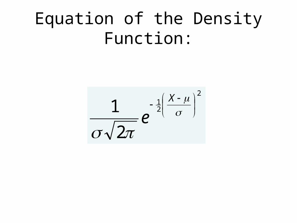
Equation of the Density Function:
2
21
2
1
X
e

According to the Germans:“That’s right on the money”
2
21
2
1
X
e

According to the Germans:“That’s right on the money”
2
21
2
1
X
e
HerrGauss

The (theoretical) proportion of people in the population
between a and b: P(a X b) = area between a and b under the curve defined by the density function.
P(a < X < b) is equal to this area
a b

THE NORMAL DISTRIBUTIONTHE NORMAL DISTRIBUTIONProperties of X ~ N( , )
The proportion of a normally distributed X within:
•one standard deviation from its mean is .6826 P( - < X < + ) = .6826
•two standard deviations from its mean is .9544 P( - 2 < X < + 2 ) = .9544
•three standard deviations from its mean is .9974 P( - 3 < X < + 3 ) = .9974
True for any value of and

Example:The population distribution of psychometric test X is a normal distribution with mean 1.1 and standard deviation of .08: Thus, X ~ N(1.1 , .08).
a) P(1.1 < X) = ?
b) P(1.02 < X < 1.18) = ?
c) How to calculate P(1.1 < X < 1.25) ?
d) How to calculate P(X > 1) ?
e) How to find x such that P(X <x) = .75 ?
0064.,08.,1.1 2
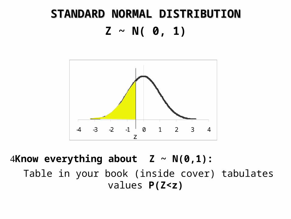
STANDARD NORMAL DISTRIBUTIONSTANDARD NORMAL DISTRIBUTION
Z ~ N( 0, 1)
-4 -3 -2 -1 0 1 2 3 4
Know everything about Z ~ N(0,1):
Table in your book (inside cover) tabulates values P(Z<z)
z

STANDARD NORMAL DISTRIBUTIONSTANDARD NORMAL DISTRIBUTION
Z ~ N( 0, 1)
-4 -3 -2 -1 0 1 2 3 4
Know everything about Z ~ N(0,1):
Table in your book (inside cover) tabulates values P(Z<z)
(note the table goes over two pages)
Note: you can think of values z of Z ~ N(0,1) as
“z many standard deviations from the mean”
z

AMAZING PROPERTY OF AMAZING PROPERTY OF
NORMAL DISTRIBUTIONSNORMAL DISTRIBUTIONS
If X is normally distributedthen a+bX (b>0) is also normally distributed.
More precisely: X ~ N( , ) (a+bX) ~ N(a+b , b)
Note:
This type of relationship is not necessarily true
for other distributions
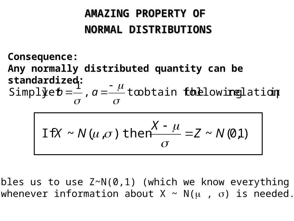
)1,0(~then ),(~ If NZX
NX
AMAZING PROPERTY OF AMAZING PROPERTY OF
NORMAL DISTRIBUTIONSNORMAL DISTRIBUTIONS
Consequence:Any normally distributed quantity can be standardized:
iprelationsh following obtain the to,1
let Simply
ab
This enables us to use Z~N(0,1) (which we know everything about) whenever information about X ~ N( , ) is needed.

Example:The population distribution of psychometric test X is a normal distribution with mean 1.1 and standard deviation of .08: Thus, X ~ N(1.1 , .08).
a) P(1.1 < X) =
b) P(1.02 < X < 1.18) =
c) How to calculate P(1.1 < X < 1.25) ?
d) How to calculate P(X > 1) ?
e) How to find x such that P(X <x) = .75 ?
0064.,08.,1.1 2

Example:The population distribution of psychometric test X is a normal distribution with mean 1.1 and standard deviation of .08: Thus, X ~ N(1.1 , .08).
a) P(1.1 < X) =
0064.,08.,1.1 2
Mean is 1.1
X~N(1.1,.08)

Example:The population distribution of psychometric test X is a normal distribution with mean 1.1 and standard deviation of .08: Thus, X ~ N(1.1 , .08).
b) P(1.02 < X < 1.18)
0064.,08.,1.1 2
Mean is 1.1
X~N(1.1,.08)
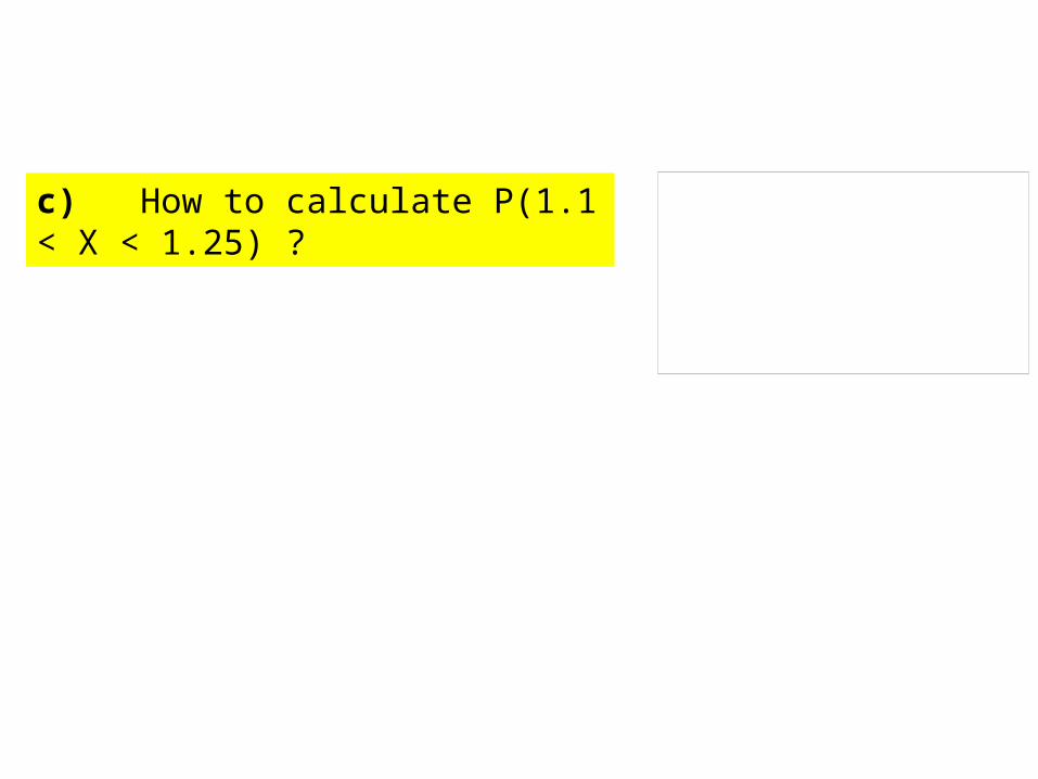
c) How to calculate P(1.1 < X < 1.25) ?
1. Draw a picture!2. Standardize:
3. Draw a picture again!4. Find the probability (using the table)
P(0<Z<1.875) =?
Example: The population distribution of psychometric test X is a normal distribution with mean 1.1 and standard deviation of .08: Thus, X ~ N(1.1 , .08).
Z~N(0,1)
X~N(1.1,.08)
1.1
0
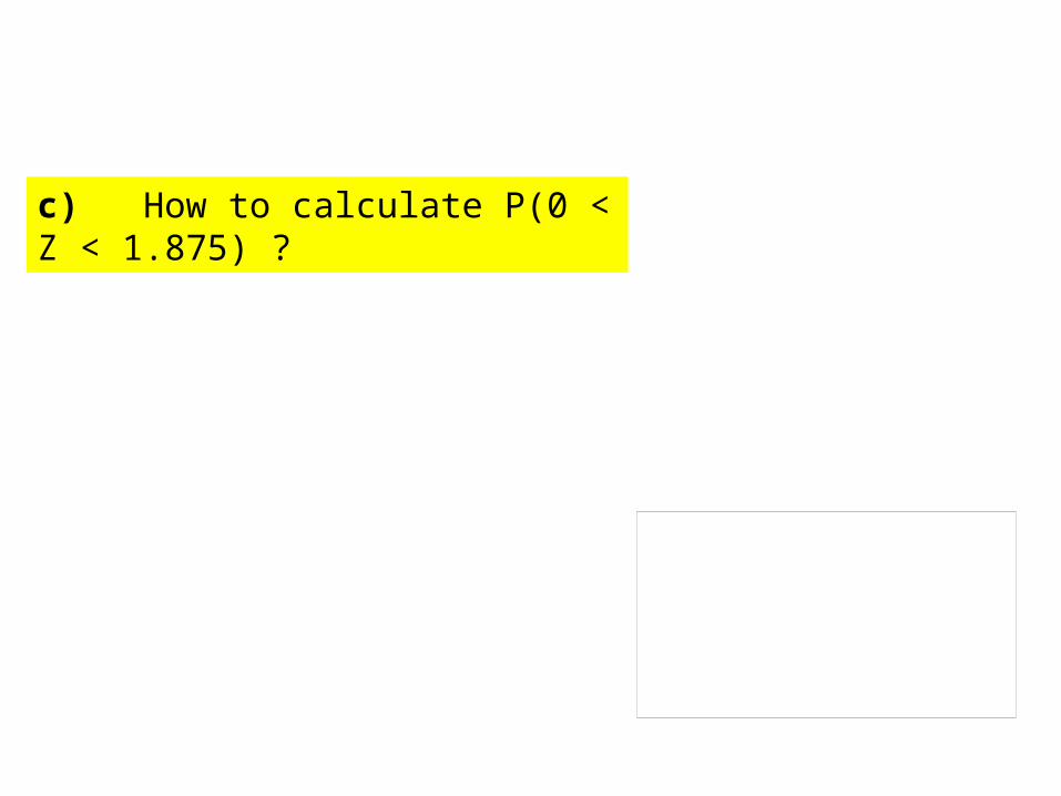
c) How to calculate P(0 < Z < 1.875) ?
Example: The population distribution of psychometric test X is a normal distribution with mean 1.1 and standard deviation of .08: Thus, X ~ N(1.1 , .08).
Z~N(0,1)
0
0
Z~N(0,1)
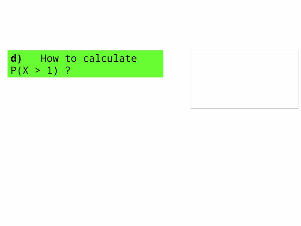
d) How to calculate P(X > 1) ?
1. Draw a picture!2. Standardize:
3. Draw a picture again!4. Find the probability (using the table)
P(Z > -1.25) =?
Example: The population distribution of psychometric test X is a normal distribution with mean 1.1 and standard deviation of .08: Thus, X ~ N(1.1 , .08).
X~N(1.1,.08)
1.1
Z~N(0,1)
0

d) How to calculate P(Z > -1.25) ?
Example: The population distribution of psychometric test X is a normal distribution with mean 1.1 and standard deviation of .08: Thus, X ~ N(1.1 , .08).
Z~N(0,1)
0
Z~N(0,1)
0

e) How to find x such that P(X < x) =.75?
1. Draw a picture!2. Standardize:
3. Draw a picture again!4. Find z (using the table)
P(Z <z)5. Solve for x using
Example: The population distribution of psychometric test X is a normal distribution with mean 1.1 and standard deviation of .08: Thus, X ~ N(1.1 , .08).
1.1
X~N(1.1,.08)
0
Z~N(0,1)