Second-order Godunov-type scheme for

reactive flow calculations on moving meshes

REPORT

Boris N. Azarenok a, Tao Tang b

aDorodnicyn Computing Center of the Russian Academy of Sciences, Vavilov str.

40, GSP-1, Moscow, 119991, Russia

bDepartment of Mathematics, The Hong Kong Baptist University, Kowloon Tong,

Hong Kong

Abstract

The method of calculating the system of gas dynamics equations coupled with the

chemical reaction equation is considered. The flow parameters are updated in whole

without splitting the system into a hydrodynamical part and an ODE part. The

numerical algorithm is based on the Godunov’s scheme on deforming meshes with

some modification to increase the scheme-order in time and space. The variational

approach is applied to generate the moving adaptive mesh. At every time step the

functional of smoothness, written on the graph of the control function, is minimized.

The grid-lines are condensed in the vicinity of the main solution singularities, e.g.

precursor shock, fire zones, intensive transverse shocks, and slip lines, which allows

resolving a fine structure of the reaction domain. The numerical examples relat-

ing to the Chapman-Jouguet detonation and unstable overdriven detonation are

considered in both one and two space dimensions.

Key words: Detonation wave, Second-order Godunov-type scheme, Moving mesh

1 Introduction

Modeling detonation wave motion in gases has started in 1940s, see, e.g., [58,26], based on

the theory of the steady one-dimensional detonation, referred to as the Zeldovich-Neuman-

Doering (ZND) model. The early computations were rather rough giving only a qualitative

Email addresses: azarenok@ccas.ru (Boris N. Azarenok), ttang@math.hkbu.edu.hk (Tao

Tang).

Preprint submitted to Elsevier Science 12th January 2005

estimate to the solution. The main difficulty of the numerical simulation is due to the

different scales of the flow domain and chemical reaction zone. Thus, the simulation for

the real objects requires using more powerful computers or more sophisticated numerical

algorithms.

Developing the numerical algorithms is executed in several ways. In the first group the

burning zone is not resolved by the grid points. Instead in [16] the chemical heat release

is put into the Riemann problem. This idea is used in [28] as well. In [15], the chemical

reaction term is present only to the energy equation, the kinetics equation is omitted and

the Riemann problem is formulated for the non-reactive gas. Although the detonation

wave speed is obtained rather inaccurately, the calculations of the real industrial objects

with complex geometry are found satisfactory. In the second group of the algorithms,

the burning zone is resolved by putting there several grid points in the normal direction.

This requires to use very fine quasiuniform meshes. In the most of these algorithms one

applies the fractional step approach (also referred to as the Strang splitting schemes).

At each time step, first, the system of conservation laws is treated and then the ODE

to the kinetics equation is solved, e.g. see [8,17,29,43,44,53]. Although the convergence

of the fractional step method was justified theoretically for scalar conservation laws with

source terms [19,52,51], the application for this approach for hyperbolic system with stiff

source terms generally produces the nonphysical solution, e.g. see [17]. Another way is to

treat the system of conservation laws coupled with the reactive equation as a whole, i.e.

using the unsplit schemes. In this approach the heat release term in the right part of the

system is treated as a source term. In [7], the generalized Riemann problem is introduced

for the reactive equations to provide the second order approximation in time. In [20], the

detonation process is simulated on the Lagrangian mesh. Space-time paths are introduced

in [42] on which the equations are reduced to the canonical form about the ”new” Riemann

invariants. All the above methods are of Godunov-type (except [16], where the random

choice method is used), i.e. include solution of the Riemann problem that allows obtaining

the narrow wave front rather precisely. In contrast to it, the random projection method

is used in [6] where the Riemann problem is omitted from the consideration. However,

justification of such a simplification is still under the question. Some other non-Godunov-

type algorithms can be found in [41].

In this work, we present an unsplit scheme for calculating the reactive flow equations

on the moving meshes. For this we utilize the idea of the Godunov’s scheme on the

deforming meshes (see the monographs [1,31]), when the conservation laws are written

in the integral form using the so-called generalized formulation in R3 space (x, y, t) (t is

time). This allows updating the flow parameters directly on the moving curvilinear mesh

without using interpolation. One implementation of the first-order Godunov’s method on

the moving mesh with front tracking was performed in [27].

In [2], a modification of the Godunov’s scheme of the second-order accuracy in time

and space was suggested, because the first-order original scheme in [31] does not provide

2

proper grid-nodes adaptation to the solution singularities. The second order in space is

achieved by interpolating the flow parameters inside the cells, and in time by using the

Runge-Kutta method with a predictor-corrector procedure. To obtain the fluxes value at

the cell faces the Riemann problem is solved. The kinetics equation is treated similarly,

namely we write it in the integral form and approximate it in the hexahedral cell in space

(x, y, t).

The variational approach is employed to generate the moving mesh. The variational ap-

proach to generate two-dimensional meshes was suggested in the form of quasi-conformal

mapping in [30]. In [55], the variational principles for constructing the adaptive moving

grids in the gas dynamics problems were formulated. They introduced the measure (or

functional) of mesh deviation from the Lagrange coordinates, measure of mesh deforma-

tion and mesh concentration. In [10], the functional of smoothness was applied, to which

the Euler-Lagrange equations coincide with the system used in [57]. In [39], the problem

of minimizing the functional of smoothness (also referred to as the harmonic or Dirich-

let’s functional) written for a surface of the control/monitor function was formulated to

construct an adaptive-harmonic mesh. Other forms of the monitor functions for the har-

monic functional have been considered in [21,11,50]. In continuous approach the harmonic

mapping, subject to some known conditions, is a homeomorphism. However, its discrete

realization, based on solving the Euler-Lagrange equations, suffers from mesh tangling in

the domains with complex geometry (e.g. nonconvex domains with singularities on the

boundary). To provide an one-to-one harmonic mapping at the discrete level, it has been

suggested in [13] to use a variational barrier method, which constructs the mapping by

minimizing the harmonic functional. The functional is approximated in such a manner

that there is an infinite barrier ensuring all grid cells to be convex quadrilaterals. In [35],

the barrier method is also used together with some geometric constrains, since in the

corners of the cell that barrier disappears. The approach from [13] has been extended

to the adaptive grid generation in [14]. In [2,3,4,5], this approach has been applied to

the two-dimensional problems of gas dynamics in nonconvex domains, where the control

function is one of the flow parameters or superposition of several parameters. In [4], the

algorithm of redistributing the boundary nodes at adaptation, consisting in constrained

minimization of the functional, was suggested. In the present work we demonstrate that

by condensing the grid lines we can better resolve main singularities in the vicinity of the

detonation wave, such as a precursor shock, fire zones, intensive transverse shocks and

slip lines.

This article has the following structure: in section 2 we will consider several aspects in

the one-dimensional case, including governing equations, boundary conditions, numerical

scheme, the Riemann problem on the moving mesh, and stability condition; the two-

dimensional case will be considered in section 3; in section 4, the grid generation method

will be presented; and in section 5, several detailed numerical simulations will be reported.

3

2 One-dimensional case

2.1 System of equations

The system of the conservation laws governing the gas flow in Euler approach and coupled

with the irreversible chemical reaction equation reads

∂σ

∂t+

∂a

∂x= c, (1)

where σ=(ρ, ρu,E, ρZ)>, a=(ρu, ρu2+p, u(E+p), ρuZ)>, and c=(0, 0, 0,−ρZK(T ))>.

Here u,p,ρ,E,T ,Z are, respectively, the velocity, pressure, density, total energy, temper-

ature, and mass fraction of the unburnt gas. The total energy is E=ρ(e+0.5u2)+qoρZ,

where e and qo are the specific internal energy and heat release, respectively. The equation

of state is p=(γ−1)eρ, where γ, the ratio of the specific heats, is assumed to be the same

in the burnt and unburnt gases. The temperature is T=p/ρR, where R is the specific gas

constant. In order that the Cauchy problem to the system (1) without chemical reaction

(added with the law of increase of the entropy s across a shock) has an unique solution,

the internal energy as a function e = e(v, s) must be convex with respect to its arguments,

i.e. the specific volume v=1/ρ and entropy s. More precisely,

evv > 0, evvess − e2vs > 0 . (2)

Moreover, e(v, s) should satisfy the additional restrictions, suggested in [56],

evs < 0, evvv < 0 . (3)

Note that till now a strict mathematical justification for uniqueness of the Cauchy problem

has not been given (only in a linearized approach, see, e.g., [32]). On the other hand the

statement of uniqueness has been confirmed by over 50 years numerical practice.

The internal energy e of the ideal gas satisfies the conditions (2) and (3). The function K,

referred to as the reaction rate, depends on the temperature T via the Arrhenius kinetics

K(T ) = Ko exp(

−E+/T)

, (4)

where E+ is the activation energy, and Ko is the rate constant. Sometimes this reaction

rate is replaced by a discrete ignition temperature kinetics model

K(T ) =

0 if T < Tign

1/τo otherwise,(5)

4

where Tign is the ignition temperature, τo is the time scale of the chemical reaction.

For the steady ZND model, we can integrate the first three ODEs in (1) and obtain

the algebraic equations connecting the values ahead and behind the Chapman-Jouguet

(CJ) detonation wave moving with the velocity DCJ [58,26]. As a result, the reactive

equation becomes the ODE for the mass fraction Z. The resulting ODE can be integrated

numerically, which yields an exact solution useful for the test modeling. This model is

also used in the case of the overdriven (also referred to as overcompressed [58]) detonation

wave.

To construct the numerical scheme on the moving mesh we will use the system (1) written

in the integral form. Integrating (1) over an arbitrary domain Ω in the x−t plane gives

∫

Ω

∫

(

∂σ

∂t+

∂a

∂x

)

dx dt =∫

Ω

∫

c dx dt .

By virtue of the Green’s theorem we get

∮

∂Ω

σ dx − a dt =∫

Ω

∫

c dx dt , (6)

where the line integration is performed along the boundary ∂Ω of the domain Ω in an

anticlock-wise manner.

2.2 Boundary conditions

Assume the detonation wave moves from the left to the right. Then ahead the wave there

is the unburnt gas and behind (strictly speaking at the infinite distance) the completely

burnt gas. Consider the matter that under what boundary conditions ahead and behind

the detonation wave then the IBVP is well posed. To understand it, we analyze the

linearized system of the gas dynamics equations written in the differential form as it is

usually performed, see, e.g., [31],

∂

∂t

ρ

u

p

+

uo ρo 0

0 uo 1/ρo

0 ρoc2o uo

∂

∂x

ρ

u

p

= 0 , (7)

5

where ρo, uo, po are the constant values, ρ, u, p are small perturbations, and co is the sound

speed. This system in a standard manner can be reduced to the canonical form

∂e

∂t+ L

∂e

∂x= 0 , (8)

where L is a diagonal matrix with the diagonal elements λ−=uo−co, λo=uo, and

λ+=uo+co. The components of the vector e=(p−ρocou, c2oρ−p, p+ρocou)> are the Riemann

invariants being constant along three characteristics dx/ dt=λ−, λo, λ+, respectively.

6

-

r

r

r

r

r

p

v

heat release Hugoniot

no reaction Hugoniot0

2

1

45

Rayleigh-Mikhel’sonline

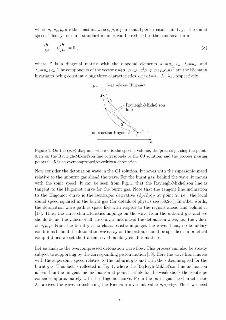
Figure 1. On the (p, v) diagram, where v is the specific volume, the process passing the points

0,1,2 on the Rayleigh-Mikhel’son line corresponds to the CJ solution; and the process passing

points 0,4,5 is an overcompressed/overdriven detonation.

Now consider the detonation wave in the CJ solution. It moves with the supersonic speed

relative to the unburnt gas ahead the wave. For the burnt gas, behind the wave, it moves

with the sonic speed. It can be seen from Fig. 1, that the Rayleigh-Mikhel’son line is

tangent to the Hugoniot curve for the burnt gas. Note that the tangent line inclination

to the Hugoniot curve is the isentropic derivative (∂p/∂ρ)S at point 2, i.e., the local

sound speed squared in the burnt gas (for details of physics see [58,26]). In other words,

the detonation wave path is space-like with respect to the regions ahead and behind it

[18]. Thus, the three characteristics impinge on the wave from the unburnt gas and we

should define the values of all three invariants ahead the detonation wave, i.e., the values

of u, p, ρ. From the burnt gas no characteristic impinges the wave. Thus, no boundary

conditions behind the detonation wave, say on the piston, should be specified. In practical

computations we set the transmissive boundary conditions there.

Let us analyze the overcompressed detonation wave flow. This process can also be steady

subject to supporting by the corresponding piston motion [58]. Here the wave front moves

with the supersonic speed relative to the unburnt gas and with the subsonic speed for the

burnt gas. This fact is reflected in Fig. 1, where the Rayleigh-Mikhel’son line inclination

is less than the tangent line inclination at point 5, while for the weak shock the isentrope

coincides approximately with the Hugoniot curve. From the burnt gas the characteristic

λ+ arrives the wave, transferring the Riemann invariant value ρocou+p. Thus, we need

6

to define its value, namely u and p on the rear boundary. In practice, one can define

only the value of u, the piston velocity. The value of p in the left endcell will be updated

automatically from the finite difference relation approximating the third equation of (8).

Generally speaking, on the rear boundary we can define the value of p. Then the velocity u

in the left endcell is updated automatically. Another question is that we do not know how

to define the pressure in the left end. We may set the value of p equal the atmospheric

pressure if it is an open end of the tube, but the overdriven detonation can not occur

in a free mode without support. On the front boundary again we should define three

conditions, i.e., the values of u, p, ρ. For the fourth reactive equation of the system (1)

the analysis is quite simple. The velocity u is the characteristic (in the linearized analysis

it is the constant value uo). It can be treated by analogy to the second equation of (8).

Therefore, we only need to define the value of Z for the unburnt gas but not for the

burnt gas (simply one uses the transmissive boundary condition). We will return to the

discussion on the rear boundary conditions at the end of this section after presenting the

numerical scheme.

2.3 Numerical scheme

In the x-t plane we introduce the moving mesh, see Fig. 2, with spacings at the nth

time level hni+1/2=xn

i+1−xni and at the n+1th level hn+1

i+1/2=xn+1i+1 −xn+1

i , and time step

∆t=tn+1−tn, where n, i are positive integers. Furthermore, for conciseness whenever pos-

sible, we will omit the superscript and subscript for the time index and use convention

that, for instance to the spacing h, using the subscript hi+1/2 denotes hni+1/2, the value at

the bottom time level n; and superscript hi+1/2 denotes hn+1i+1/2, the value at the top time

level n+1.

6

b b

bb

n+1

n+1/2

ni i+1/2 i+1

t

xr

r r

r

-1 2

Figure 2. A quadrilateral (trapezoidal) cell Ωn+1/2

i+1/2in the x-t plane, which corresponds to two

states of the control volume (xi, xi+1) at time tn and tn+1, respectively.

Let at time tn the initial vector-valued function f i+1/2 = (u, p, ρ, Z)>i+1/2 be known at each

7

zone mid point xni+1/2, where, for instance, ui+1/2 is the cell-average value of the velocity

ui+1/2 =1

hi+1/2

xn

i+1∫

xn

i

u(x, tn) dx.

Consider the control volume (xi, xi+1) at time tn and tn+1. We can draw conceptually the

quadrilateral cell Ωn+1/2

i+1/2 in the x-t plane, see Fig. 2. Integrating the system (6) along the

contour ∂Ωn+1/2

i+1/2 , we obtain the system of the finite difference equations

σi+1/2hi+1/2 − σi+1/2hi+1/2 − σi+1hi+1 + σihi + ∆t(ai+1 − ai) =

12∆t(hi+1/2 + hi+1/2)c

n+1/2

i+1/2 , (9)

where the value of σi+1/2 is taken at point xn+1i+1/2, σi and σi+1 at x

n+1/2i and x

n+1/2i+1 ,

respectively; hi=xn+1i −xn

i is the projection of the lateral edge xni x

n+1i (further referred to

as the ith lateral edge) onto the x-axis. The function cn+1/2

i+1/2 is taken in the center of the

quadrilateral cell. The Eqs. (9) can be interpreted as a discrete form of the conservation

laws on the moving mesh. Actually, the change of the vector-valued function σ in the

control volume (xi, xi+1) within time ∆t (first two terms in the left-hand side of (9)) is

due the following: motion of the segment endpoints xi and xi+1 (third and fourth terms);

convection (fifth term); and internal source (right-hand side term).

To update the cell average values f i+1/2 via (9) with the second order of accuracy one

needs to know the fluxes through the endpoints, in other words the values f i,f i+1 at time

tn+1/2. We will apply the predictor-corrector procedure. Besides, one assumes the vector-

valued discrete function f to be piece-wise linear within the control volume (xi, xi+1).

At the first stage, predictor, in (9) we set f i=f 1,i+1/2, and f i+1=f 2,i+1/2, i.e. take those

values at the lateral edges at time tn (superscript n is omitted) instead of at tn+1/2. To find

the values at the left and right zone ends, i.e., f 1,i+1/2, and f 2,i+1/2 (see Fig. 2), we use

the interpolation involving a monotonicity procedure [2,5]. Note that many interpolation

procedures can be used here, for instance, minmod [38] reformulated on the nonuniform

mesh. All of them provide rather similar results for the discontinuous solutions (especially

on the curvilinear mesh in the two-dimensional case). Actually we find some ”effective”

derivatives δf i+1/2 which are used to calculate the values at the zone ends

f 1,i+1/2 = f i+1/2 − 0.5δf i+1/2hi+1/2 , f 2,i+1/2 = f i+1/2 + 0.5δf i+1/2hi+1/2 . (10)

We also set cn+1/2

i+1/2 =cni+1/2. Therefore, the intermediate values f

i+1/2at the n+1th level

can be updated using (9).

Next, at the second stage, corrector, we obtain the pre-wave values of f at the lateral

8

edges i and i+1 at time tn+1/2. With this purpose we set the effective derivatives at tn+1

equal to the ones at tn [45], i.e. δfi+1/2

=δf i+1/2. Then at tn+1 the values at the zone

ends for the intermediate function fi+1/2

are obtained from the relations similar to (10).

Taking the mean of the zone ends values at tn and tn+1 we obtain the pre-wave states at

the lateral edges i and i+1 at time tn+1/2 as follows:

fn+1/2

1,i+1/2 = 0.5[

f i+1/2 +fi+1/2

− 0.5δf i+1/2(hi+1/2 + hi+1/2)]

,

fn+1/2

2,i+1/2 = 0.5[

f i+1/2 +fi+1/2

+ 0.5δf i+1/2(hi+1/2 + hi+1/2)]

. (11)

Knowing the pre-wave values fn+1/2

2,i−1/2 and fn+1/2

1,i+1/2 from the both side of every point xi,

one obtains the endpoints values fn+1/2i and f

n+1/2i+1 by solving the Riemann problem (see

section 2.4 below). Now we can calculate the values σi,σi+1,ai, and ai+1. Substituting

them into Eqs. (9) gives the final values f i+1/2.

The above described scheme is second-order accurate in both space and time provided

that the solution is smooth in the entire flow domain and the mesh is quasiuniform [2],

i.e.

hi+1/2 − hi−1/2 = O((hi+1/2)2) .

2.4 Riemann problem on the moving mesh

In the calculations we assume the detonation wave to be resolved by several grid points

located in the burning zone. On the Rayleigh-Mikhel’son line the burning zone is enclosed

between the points 1 and 2 (or 4 and 5), see Fig. 1. Thus, we work with the model

corresponding to the real physical process, where the heating shock moves first and behind

it is the burning zone. In this model, we can use the Riemann solver developed for the

non-reactive gas, because at point 1 (or 4), immediately behind the precursor shock, the

reaction has not taken place yet.

We apply the Riemann solver developed by Prokopov [31] based on the exact solution of

the nonheating PDE system (for description of this Riemann solver see also [36]). The

“exact solution” means that we determine accurately the wave pattern emerging after

left-side and right-side gases (each with constant parameters) begin to interact.

To demonstrate how to take into account the grid nodes movement let us consider the ith

lateral edge of the cell Ωn+1/2

i+1/2 within the time interval from tn+1/2 to tn+1. Assume that

after solving the Riemann problem at point xn+1/2i we have the wave pattern depicted in

Fig. 3. There are 5 cases for the location of the segment (xn+1/2i , xn+1

i ), or the upper half

of the ith lateral edge, in the wave pattern depending on the velocity wi of the ith node.

9

As for the post-wave values fn+1/2i (except Z

n+1/2i ), we take:

1. fn+1/2i = f

n+1/2

2,i−1/2 if wi < dsh, where dsh is the speed of the left shock.

2. fn+1/2i = f 2 if dsh < wi < dcont, where the vector f 2 defines the flow parameters

behind the shock, dcont is the speed of the contact discontinuity which equals to the

velocity u in that domain.

3. fn+1/2i = f 3 if dcont < wi < dlft

rar, where the vector f 3 defines the parameters in

the domain between the contact discontinuity and left characteristic of the rarefaction

wave expanding with the speed dlftrar.

4. fn+1/2i = φ(x/t) if dlft

rar < wi < drghtrar , i.e. we calculate the flow parameters in the

rarefaction wave using the similarity variable x/t. Here drghtrar is the speed of the right

characteristic in the rarefaction fan.

5. fn+1/2i = f

n+1/2

1,i+1/2 if wi > drghtrar .

Note that in [31] the above algorithm is applied at time tn.

-

6t

x

shock

contactdiscont.

rarefac.fan

fn+1/2

2,i−1/2f

n+1/2

1,i+1/2r

r

i, n+1/2

r

rr

r

1

2

3 4

5

Figure 3. Five possible cases of location of the segment (xn+1/2i , xn+1

i ) in the wave pattern. Points

1, . . ., 5 indicate location of the ith node at tn+1.

-

t

x

contactdiscont.

Zn+1/2

2,i−1/2Z

n+1/2

1,i+1/2r

i, n+1/2

r r

1 2

6

Figure 4. Two possible cases of location of the segment (xn+1/2i , xn+1

i ) in the wave pattern for

the chemical reaction equation.

For the reactive equation, since the characteristic is dx/ dt=u, we use the jump condition

10

to find the post-wave value Zn+1/2i , see Fig. 4, namely

Zn+1/2i =

Zn+1/2

2,i−1/2 if wi < dcont

Zn+1/2

1,i+1/2 otherwise.(12)

In the center of the quadrilateral cell we approximate the flow parameters by

fn+1/2

i+1/2 = 0.5(f i+1/2 +fi+1/2

).

At last, we update the final values f i+1/2 at time tn+1 by using (9).

2.5 Stability condition

In the one-dimensional case the choice of the admissible time step ∆t has a clear physical

sense. On the moving grid ∆t is given by

∆t = ccfl mini

∆ti+1/2, (13)

where in every cell the local time step is determined by (cf. [31])

∆ti+1/2 =hi+1/2

max(drghti − wi+1 , −dlft

i+1 + wi). (14)

Here drghti and dlft

i+1 are the extreme right and left wave speeds at points xi and xi+1,

respectively, obtained by solving the Riemann problem, and wi is the velocity of the node

xi. The condition (14) means that we estimate the time within which the left characteristic

(in the linearized analysis this is a straight line), emanating from the i+1th node, achieves

the ith node, as well as the time within which the right characteristic, emanating from

the ith node, achieves the i+1th node. From these two time steps we take the minimal.

If in some cell ∆ti+1/2<0 (on the moving mesh it can happen), we exclude this cell from

consideration in (13). The condition (14) covers the stability condition for the kinetic

equation as well, because here the characteristic extends with the speed of the contact

discontinuity. The CFL number ccfl (or coefficient of reserve [31]) is a correction to the

non-linearity of the PDE system. To calculate the node velocity wi, on one hand it is

necessary to know the time step ∆t, and on the other hand wi participates in determining

∆t. By this reason at time level n+1 we use ∆t obtained at the preceding level n. The

coefficient ccfl<1, usually about 0.5, may be corrected during the computation.

11

In the linearized analysis on the fixed grid we use a sound approach to get ∆ti+1/2 in each

cell

∆ti+1/2 =hi+1/2

max(ui+1/2 + ci+1/2 , −ui+1/2 + ci+1/2)(15)

where the sound speed is equal to c2i+1/2=γ(p/ρ)i+1/2. The formula (15) can be also used

if the mesh-moving speed is not too high.

Let us return to the matter on prescribing the boundary conditions at the end of the

reaction zone. Besides the ‘piston’ condition, for instance in [37] for the linear stability

analysis the ‘radiation’ condition is also applied. It requires that there is no perturbation

to the steady state at the end of the reaction zone that travels forward, towards the

detonation wave from the piston. This, in turn, implies that the third equation in (7) is

excluded by assuming its linear dependence on the first and second ones. However, such a

condition can not be used in nonlinear calculations for the following reason. Assuming the

flow is smooth at the end of the reaction zone, the numerical scheme can be constructed

by approximating the PDEs in the nondivergent form (7) and, therefore, by treating (8).

Now ρo and co are the frozen coefficients in the numerical procedure defined by initial

data at the predictor and corrector steps and depending on the coordinates x, y. We can

not eliminate the invariant p+ρocou influence on the forward solution. It would mean

the third equation be excluded from the system (8). Besides, the overcompressed steady

detonation mode is only possible under the support provided by this invariant [58]. The

unstable detonation mode, which will be considered in sections 5.2 and 5.3, is only a

deviation of the basic steady state. Thus, one can only prescribe the invariant value at

the left endpoint. Due to the truncation errors this invariant always transfers pertrubation

to the forward state. The above analysis is valid also when the third equation of (7) is

inhomogeneous with the chemical term in the right-hand part.

3 Two-dimensional case

3.1 System of equations

The governing system of the differential equations relating to the two-dimensional reactive

gas flow is

∂σ

∂t+

∂a

∂x+

∂b

∂y= c , (16)

where σ = (ρ, ρu, ρv, E, ρZ)>, a = (ρu, ρu2+p, ρuv, u(E+p), ρuZ)>,

b = (ρv, ρuv, ρv2+p, v(E+p), ρvZ)>, c = (0, 0, 0, 0,−ρK(T )Z)>, u and v are the velocity

12

components. Now the total energy becomes E = ρ[e + 0.5(u2 + v2)] + qoρZ .

We perform calculations utilizing the integral conservation laws which can be derived by

integrating the system (16) and transforming the volume integrals in R3 space (x, y, t) to

the surface integrals with the use of the Gauss’s theorem

∫ ∫

Ω

∫

[

∂σ

∂t+

∂a

∂x+

∂b

∂y− c

]

dΩ =∫

∂Ω

∫

©σ dx dy +a dy dt+b dt dx−∫ ∫

Ω

∫

c dx dy dt = 0 .

Here the domain Ω with the boundary ∂Ω is a homeomorphic sphere in space (x, y, t), see

Fig. 5. Hence, the system can be rewritten in the integral form as follows (such generalized

formulation for the nonreactive gas flow has been suggested in [31])

∫

∂Ω

∫

© σ dx dy + a dy dt + b dt dx =∫ ∫

Ω

∫

c dx dy dt. (17)

-

6

x

y

t∂1Ω

∂oΩ

∂′ΩΩ

Figure 5. Domain Ω in space (x, y, t) with the boundary ∂Ω = ∂oΩ ∪ ∂1Ω ∪ ∂′Ω. Here ∂oΩ and

∂1Ω is the underlying control volume in the x-y plane at time to and t1, respectively.

The meaning of this form is the following. The boundary ∂Ω of the underlying domain

consists of three parts: ∂Ω = ∂oΩ ∪ ∂1Ω ∪ ∂′Ω. The amount of the parameters (mass,

momentum, total energy, and reactant mass) in the two-dimensional domain, a control

volume ∂oΩ, at time to is equal to

∫

∂oΩ

∫

σ dx dy.

Since the control volume boundary moves, by time t1 the domain ∂oΩ becomes ∂1Ω and

the corresponding amount changes to

∫

∂1Ω

∫

σ dx dy.

The change of the parameters is due to the flux through the moving boundary of the

control volume and the surface stresses (to the momentum and energy equations), which

can be expressed as follows:

∮

C

a dy + b dx.

13

Here the contour C is the boundary of the two-dimensional control volume in the x-y

plane, which changes with time. At t=to the contour C is the boundary of the control

volume ∂oΩ and at t=t1 of ∂1Ω. The change of the parameters within the time (to, t1) is

t1∫

t0

∮

C

(a dy + b dx) dt =∫

∂′Ω

∫

(a dy + b dx) dt.

Furthermore, we should take into account the reactant mass change due to burning, caused

by the source term in the right-hand side of (16). To this end, we formulate the integral

conservation laws as follows. The change of the flow parameters (mass, momentum, total

energy, or reactant mass) in the control volume is due to the flux through the moving

boundary of the control volume, surface stresses, and internal sources

∫

∂1Ω

∫

σ dx dy −∫

−∂oΩ

∫

σ dx dy +∫

∂′Ω

∫

(a dy + b dx) dt =∫ ∫

Ω

∫

c dx dy dt,

where the sign ”-” with ∂oΩ indicates the change of the domain orientation. This system

can be rewritten in the brief form (17). The integral conservation laws extends the class

of admissible functions since it is not required that the solution to be differentiable as in

(16), and it governs the discontinuous solutions as well.

Of course, logically we should begin the governing equations derivation with the integral

form (17), since the system (16) is a consequence of (17). However, the form (16) is more

habitual and that is why it is presented first.

3.2 Numerical scheme

We introduce the curvilinear moving grid in the x-y plane, and the (i+1/2, j+1/2)th cell

at time tn and tn+1 is shown Fig. 6. We draw mentally a domain Ω in R3 space (x, y, t),

being a hexahedron with planar top and bottom faces and four ruled lateral faces.

The bottom face of the hexahedron Ω is the control volume at time tn and the top face at

tn+1. Integrating (17) over the oriented surface, i.e. the boundary ∂Ω of the hexahedron,

gives a cell-centered finite-volume discretization of the governing equations

σi+1/2,j+1/2A1′2′3′4′ − σi+1/2,j+1/2A1234 + Q411′4′ + Q233′2′ + Q122′1′ + Q344′3′ =

cn+1/2

i+1/2,j+1/2Ω, (18)

where σi+1/2,j+1/2 and σi+1/2,j+1/2 are the average values at time tn+1 and tn in the

center of the top and bottom faces, respectively; A1′2′3′4′ and A1234 are the areas of the

14

-

6

x

y

t

n

n+1

1 4

32

2′ 3

′

1′

4′

i, j i, j+1

i+1, j i+1, j+1

r

r

2′′

1′′

Figure 6. Hexahedron Ω in R3 space with bottom (1234) and top (1’2’3’4’) faces, being the cell

of the 2D moving mesh at time tn and tn+1, respectively.

corresponding faces. Each of the four vector values Q411′4′ , Q233′2′ , Q122′1′ and Q344′3′ is

the amount of the mass, momentum, energy, and reactant mass which flows into and out

the quadrilateral cell 1234 within time ∆t through the corresponding moving edges of the

cell. The value cn+1/2

i+1/2,j+1/2 is defined in the center of the hexahedron (in other words in

the center of the quadrilateral cell at tn+1/2), and Ω is the hexahedron volume.

For example, Q122′1′ , the change of the parameters due to the flux through the edge 12

within time ∆t, is given by

Q122′1′ = σn+1/2

i+1/2,jAxy122′1′ + a

n+1/2

i+1/2,jAyt122′1′ + b

n+1/2

i+1/2,jAtx122′1′ , (19)

where σn+1/2

i+1/2,j ,an+1/2

i+1/2,j , and bn+1/2

i+1/2,j are calculated using the parameters f = (u, v, p, ρ)>

in the center of the face 122′1′, i.e. at the mid-point of edge 12 at time tn+1/2 (or at the

mid-point of edge 1′′2′′); Axy122′1′ , Ayt

122′1′ , Atx122′1′ are the areas of the projections of the face

122′1′ onto the coordinate planes x-y, y-t, and t-x, respectively, given by

Axy122′1′ =

∫ ∫

122′1′

dx dy = 0.5[(x2′ − x1)(y1′ − y2) − (x1′ − x2)(y2′ − y1)],

Ayt122′1′ =

∫ ∫

122′1′

dy dt = 0.5∆t(y2′ + y2 − y1 − y1′),

Atx122′1′ =

∫ ∫

122′1′

dt dx = −0.5∆t(x2′ + x2 − x1 − x1′).

These expressions are obtained from the formula for the quadrangle 1234

A1234 = A(x1, y1; x2, y2; x3, y3; x4, y4) = 0.5[(x3 − x1)(y4 − y2) − (x4 − x2)(y3 − y1)] ,

when passing its contour in an anticlock-wise manner.

15

As in the one-dimensional case, the values f i+1/2,j+1/2 are updated by two stages using a

predictor-corrector procedure. At the first stage, predictor, we compute the intermediate

values at the n+1th level fi+1/2,j+1/2

by using (18).

Let us consider the curvilinear coordinate ξ. Assume the function f to be linear within

the cell (i+1/2, j+1/2) in the ξ-direction. The values f i,j+1/2 and f i+1,j+1/2, specified at

the left and right ends of the segment ((i, j+1/2), (i+1, j+1/2)) at tn, are defined via

f i,j+1/2 = f i+1/2,j+1/2 − 0.5δf i+1/2hi+1/2 ,

f i+1,j+1/2 = f i+1/2,j+1/2 + 0.5δf i+1/2hi+1/2 . (20)

Here δf i+1/2 is the ”effective” derivative in the ξ-direction, and the spacing hi+1/2 is the

length of the underlying segment. Note that δf i+1/2 and hi+1/2 are the short notations for

(δf ξ)i+1/2,j+1/2 and (hξ)i+1/2,j+1/2, respectively. When determining δf i+1/2, to suppress

spurious oscillations in the vicinity of discontinuities the monotonicity algorithm should

be applied as that of in the one-dimensional case. The spacing hi+1/2 is given by

hi+1/2 = 0.5√

(xni+1,j + xn

i+1,j+1 − xni,j − xn

i,j+1)2 + (yn

i+1,j + yni+1,j+1 − yn

i,j − yni,j+1)

2.

By analogy we calculate the values f i+1/2,j and f i+1/2,j+1, which are specified at the left

and right ends of the segment in the η-direction in the cell. Note, since we interpolate f

along the curvilinear coordinate lines ξ and η, in general, the order of interpolation is less

then 2, and equal 2 only if the mesh is rectangular.

We substitute the determined values of f at the mid-point of the lateral edge 12 of the

quadrilateral 1234, i.e. at time tn instead of the ones at time tn+1/2, in (19) to find the

values Q122′1′ . The values Q411′4′ , Q233′2′ , and Q344′3′ can be found in a similar way. For

the parameter cn+1/2

i+1/2,j+1/2 we use the one at time tn. A good approximation to the volume

Ω is given by

Ω = 0.5(A1′2′3′4′ + A1234)∆t.

Finally, from (18) we obtain the intermediate values fi+1/2,j+1/2

at the n+1th level.

We now discuss the second stage, corrector. As in the one-dimensional case we obtain the

values in the center of the faces 122′1′ and 344′3′, i.e. at the mid-point of the edges 12

and 34 at time tn+1/2 :

fn+1/2

i,j+1/2 = 0.5[

f i+1/2,j+1/2 +fi+1/2,j+1/2

− 0.5δf i+1/2(hi+1/2 + hi+1/2)]

,

fn+1/2

i+1,j+1/2 = 0.5[

f i+1/2,j+1/2 +fi+1/2,j+1/2

+ 0.5δf i+1/2(hi+1/2 + hi+1/2)]

,

where the spacing hi+1/2 is the length of the segment ((i, j+1/2), (i+1, j+1/2)) at time

tn+1. We can obtain fn+1/2

i+1/2,j and fn+1/2

i+1/2,j+1 in a similar way. These four vector values

16

are used as the pre-wave states in the center of the corresponding lateral faces of the

hexahedron for the Riemann problem.

Let us consider the face 122′1′. To get the postwave states fn+1/2 in the center of this face

(for brevity we omit subscripts), i.e. at the mid-point of the segment (1′′, 2′′), we solve

the Riemann problem with the pre-wave states (r, p, ρ)n+1/2 at this point on both sides of

the face (one state relates to the underlying hexahedron and the other to the hexahedron

adjacent to the face 122′1′). Here rn+1/2 is the normal component of the velocity to the

segment (1′′, 2′′). We also use the tangential components of the velocity qn+1/2 on those

sides. The normal and tangential components of the velocity are given by

rn+1/2 = nxun+1/2 + nyv

n+1/2 , qn+1/2 = nyun+1/2 − nxv

n+1/2 ,

where nx, ny are the components of the outward unit normal vector to the segment (1′′, 2′′).

After solving the Riemann problem, the post-wave values (r, p, ρ)n+1/2R in the face center

are defined. The post-wave tangential component of the velocity qn+1/2R is given by

qn+1/2R =

qn+1/2 if w12 ≤ dcont ,

qn+1/2 otherwise ,(21)

where dcont is the contact discontinuity speed in the Riemann problem, w12 is the velocity

of the edge 12 in the normal direction to this edge, and qn+1/2 is the pre-wave tangential

component of the velocity in the hexahedron adjacent to the face 122′1′. This condition

expresses the fact that the tangential component of the velocity is discontinuous across

the tangential discontinuity, cf. [18]. The velocity w12 can be derived from the equality

∆tl1′′2′′w12 = Axy

122′1′ , (22)

where l1′′2′′ is the length of the segment (1′′, 2′′). Next we restore the Cartesian components

of the post-wave velocity in the center of the face 122′1′

un+1/2R = nxr

n+1/2R + nyq

n+1/2R , v

n+1/2R = nyr

n+1/2R − nxq

n+1/2R .

We treat the mass fraction Z using (12) and find Zn+1/2R on this face.

Given the post-wave values (u, v, p, ρ, Z)n+1/2R in the center of the face 122′1′, we calculate

Q122′1′ via (19). Similarly we treat the Riemann problem in the center of the other three

faces to obtain Q411′4′ , Q233′2′ , and Q344′3′ . When calculating cn+1/2

i+1/2,j+1/2, the values of

fn+1/2

i+1/2,j+1/2 are given by

fn+1/2

i+1/2,j+1/2 = 0.5(

f i+1/2,j+1/2 +fi+1/2,j+1/2

)

.

17

The final values of f i+1/2,j+1/2 at time tn+1 are obtained by using (18).

3.3 Stability condition

In the 2D case the choice of the admissible step ∆t may be estimated in the energetic

norm to the underlying Eqs. (16), written as a t-hyperbolic by Friedrichs’s system [31].

The step ∆t for nonreactive gas flow calculation in the (i+1/2, j+1/2)th cell is given by

∆ti+1/2,j+1/2 =∆t

′

∆t′′

∆t′ + ∆t′′, (23)

where

∆t′

=h

′

max(dright14 − w23;−dlft

23 + w14), ∆t

′′

=h

′′

max(dright12 − w34;−dlft

34 + w12), (24)

h′

=A1234

0.5√

(x4 + x3 − x1 − x2)2 + (y4 + y3 − y1 − y2)2,

h′′

=A1234

0.5√

(x3 + x2 − x4 − x1)2 + (y3 + y2 − y4 − y1)2.

Here ∆t′

and ∆t′′

are the admissible time steps to the one-dimensional scheme in the ξ

and η-direction, respectively; h′

, h′′

are the “average heights” of the bottom face 1234,

and w is the velocity of the corresponding cell edge. For example, w12 is the velocity of

the edge 12 in the normal direction determined via (22). Next, dright12 and dright

14 are the

“extreme right wave” speeds defined from solving the Riemann problem to the faces 122′1′

and 11′4′4, respectively; dlft23 and dlft

34 are the “extreme left wave” speeds to the faces 233′2′

and 433′4′, respectively.

The resulting time step over the mesh is given by

∆t = ccfl mini,j

∆ti+1/2,j+1/2

3.4 Front tracking

Now we turn to describe the front tracking procedure drawn in [31]. The front of the

detonation wave is the precursor heating shock. Therefore, its velocity should be deter-

mined by using the Rankine-Hugoniot jump conditions, in other words from the Riemann

problem solved on the cell edges located on the moving part of the domain boundary ∂Ω

at time tn+1/2. At the predictor stage we use the mesh taken from the preceding time level

tn.

18

r

r r

r

r

]

6

Bi−1

Bi Bi+1

B′i

B′′i

w∗

i−1/2

w∗

i+1/2i−1

ii+1

ϕ′i

ϕ′′i

Figure 7. Front tracking for the heating shock wave.

Consider two those edges Bi−1Bi and BiBi+1, see Fig. 7. We must define the directions

along which the boundary nodes i−1, i, i+1 move (for brevity we use only one subscript

i). After solving the Riemann problem at the mid-point of these two edges we obtain the

speed of extreme left (or right) characteristics, which are used as the normal velocities

w∗i−1/2, w

∗i+1/2 for these edges. The velocity of the ith node along the ith direction can be

determined by two ways. First, as the velocity of the end-point Bi in the edge Bi−1Bi

w′

i =w∗

i−1/2

cos ϕ′i

,

where ϕ′i is the angle between the velocity vector w∗

i−1/2 (that is a normal vector to the

edge Bi−1Bi) and direction i. In Fig. 7, the value of w′i is indicated by the segment (Bi, B

′i).

The second velocity of the ith node along the ith direction is determined as the velocity

of the end-point Bi in the edge BiBi+1

w′′

i =w∗

i+1/2

cos ϕ′′i

.

In Fig. 7, the value of w′′i is indicated by the segment (Bi, B

′′i ). As the velocity of the ith

node in the direction i we use the interpolated value

w∗

i = w′

i

li+1/2

li−1/2 + li+1/2

+ w′′

i

li−1/2

li−1/2 + li+1/2

,

where

li+1/2 =√

(xni+1 − xn

i )2 + (yni+1 − yn

i )2 .

Afterwards the position of the ith boundary node at time tn+1 is given by

xn+1i = xn

i + w∗

x,i∆t , yn+1i = yn

i + w∗

y,i∆t ,

where w∗x,i, w

∗y,i are the components of the velocity vector w∗

i .

19

3.5 Discussion on accuracy

As in the one-dimensional case this scheme is second-order accurate in both space and

time provided that the solution is smooth in the entire flow domain and the mesh is

quasiuniform and close to rectangular. In real applications, however, the smoothness of

the flow is violated even if initially it was so. The flow parameters and their derivatives

suffer discontinuity across the singularities: shock, contact discontinuity, and rarefaction

wave extreme left and right characteristics. Thus, the linear interpolation (10) or (20),

constructed via the Taylor expansion to the underlying functions, is generally incorrect for

determining the fluxes at the cell boundaries, that is, the order of weak convergence falls in

the entire flow domain. This effect was observed by Godunov at the end of 1950s [33]. The

first order Godunov’s scheme in the smooth domain of the rarefaction wave exhibited the

weak convergence rate r≈2/3 instead of 1 as it is followed from the formal approximation of

the system of equations. For high-order schemes, the reduction of accuracy in the smooth

subdomains in the presence of shocks was also observed, for instance, in [40,12,22]. In [2],

the present scheme was tested in the shock tube problem with the flow pattern consisting

of the shock, contact discontinuity, and rarefaction fan. When tracking the extreme left

and right characteristics and calculating within the rarefaction fan only, the convergence

rate r is 2 in the L1 norm and is close to 2 in the L∞ norm. However, when calculating

the entire flow domain with this scheme in the shock capturing manner, it falls down to

1 (in L1 norm) even if to estimate r only within the rarefaction wave, where the flow

is smooth. From the standpoint of numerical calculations this effect can be explained as

follows. In the vicinity of the singularity, due to the use of the limiter, in several cells

(usually in two) the order of approximation falls down to 1. This is because the piecewise

linear reconstruction inside the cell is changed to piecewise constant. In addition, in one

of these two cells the scheme may be even unconditionally unstable [45]. This leads to

the disturbances from those cells that extend along the characteristics into subdomains

of the smooth flow and they deteriorate the accuracy of the solution. Thus the term

”second-order” is rather conditional. The remedy to support the high accuracy is to fit

every shock by a special shock fitting procedure, which treat the discontinuities using the

Rankine-Hugoniot jump conditions. Examples of such calculations will be presented in

sections 5.2 and 5.3. One more way to prevent accuracy deterioration in the presence of

shocks is to use the adaptive meshes. This effect will be discussed in section 5.3.

If the ”second-order” scheme only yields first-order results, why use it? We keep in mind

two reasons. The first one is obvious. The second-order error is significantly smaller than

the first-order one. In [4], we performed calculations of the steady supersonic gas flow in

the channel, where several oblique shocks divide the flow into subdomains with a known

exact solution, by using four successively refined quasiuniform meshes. The present scheme

exhibited the convergence rate r=0.92 to 0.96, while the first-order scheme gave r=0.35

to 0.68. The second reason is that we aim to use the adaptive mesh coupled with the flow

solver. Treating the one-dimensional flow on the moving meshes with the first- and second-

20

order schemes increases significantly the accuracy relatively to fixed mesh calculation [4].

In the two-dimensional flow, our scheme on the adaptive meshes increases the accuracy

by factors up to 5, while the first-order scheme does not provide enhancement at all.

4 Grid generation

The variational approach is employed to generate the moving adaptive mesh. It is from

the class of so-called r-refinement methods. There is one more class of the adaptive mesh

method, so called h-refinement, which is outside of the present study.

4.1 Problem formulation

-

6

x

y

z

-

6η

ξdomain Ω

x(ξ, η), y(ξ, η)

Harmonicmapping

surface f(x, y)

parametricdomain

Projection

? j

Figure 8. Adaptive grid generation.

The regular adaptive-harmonic mesh is constructed by minimizing the harmonic func-

tional written for a surface of the control/monitor function f(x, y) [39]. The relevant

notations are shown in Fig. 8. The functional defining the adaptive grid, clustered in

regions of large gradients of the function f , is (for derivation see [14,4])

I =∫ ∫ (x2

ξ + x2η)(1 + f 2

x) + (y2ξ + y2

η)(1 + f 2y ) + 2fxfy(xξyξ + xηyη)

(xξyη − xηyξ)√

1 + f 2x + f 2

y

dξ dη . (25)

The problem of grid adaptation is formulated as follows. Let in the parametric domain

the coordinates of the grid nodes be given, which is formed by square elements. Given the

mapping of the parametric domain boundary onto the domain boundary ∂Ω, we seek a

harmonic mapping of the surface Sr2 of the graph of f(x, y) onto the parametric domain,

by minimizing the functional (25). In the results we obtain the quasiuniform mesh on

the surface Sr2, which, being projected onto Ω, defines the adaptive mesh in the physical

domain Ω. Subject to some known conditions, e.g. see [47], such a harmonic mapping exists

21

and is a homeomorphism (one-to-one and onto). In unsteady problems such a formulation

is considered at every time step.

In the 1-D case, to generate the inverse mapping of the graph of f onto the segment on

the parametric axis ξ requires us to minimize the following functional (see [39]):

I =∫ 1

xξ

√

1 + f 2x

dξ. (26)

With the purpose of controlling the degree of grid condensing in the domains of large

gradients, it is convenient to use caf instead of f , where ca is a coefficient of adaptation,

which can depend on the variables x, y. Thus, we work with the control function multiplied

by some coefficient ca in order to increase or decrease adaptation.

4.2 Minimization of the functional

The functional (25) is approximated in such a way that its minimum is attained on a grid

of convex quadrilaterals, referred to as a convex grid [14,5],

Ih =imax∑

i=1

4∑

k=1

1

4[Fk]i , (27)

where Fk is the integrand evaluated in the kth corner of the ith cell. If the set of convex

meshes is not empty, the system of the algebraic equations written at every interior node

Rx =∂Ih

∂xi

= 0, Ry =∂Ih

∂yi

= 0, (28)

where i is a global node number, has at least one solution that is a convex mesh. To find it

an initial convex mesh should be given and an unconstrained minimization method needs

to be used. Assuming the grid is convex at the pth iteration step we find the coordinates

of the ith node at the p+1th step using the quasi-Newton method (see [14,5] for details):

xp+1i = xp

i − τ

(

Rx∂Ry

∂yi

− Ry∂Rx

∂yi

)(

∂Rx

∂xi

∂Ry

∂yi

−∂Ry

∂xi

∂Rx

∂yi

)−1

,.

yp+1i = yp

i − τ

(

Ry∂Rx

∂xi

− Rx∂Ry

∂xi

)(

∂Rx

∂xi

∂Ry

∂yi

−∂Ry

∂xi

∂Rx

∂yi

)−1

, (29)

where the iterative parameter is 0 < τ ≤ 1.

When generating a curvilinear mesh without adaptation in the physical domain Ω (if no

adaptation, we substitute fx=fy=0 in (25)), the discrete functional (27) has an infinite

22

barrier on the boundary of the set of convex grids [13,14]. This is caused by the condition

of positiveness to the Jacobian of the mapping J=xξyη−xηyξ. This property allows for

generating the unfolded mesh in domains of any geometry. When adapting, due to dis-

continuities in the solution the infinite barrier disappears [4], which causes some grid cells

to fold and modeling to break. To prevent it, first, we use a regularization procedure to

the discrete functional [4]. The second way was suggested in [3] for unsteady problems.

We specify Dmax, the maximal value of the modulus of the gradient of f , as follows

Dmax=λ max(|∇f |) ,

where f=cafh, fh is an interpolant of f , the coefficient λ<1 and |∇f |=

√

f 2x + f 2

y . Next,

the gradient of the function is updated via

∇f ∗ =

Dmax∇f/|∇f | if |∇f | > Dmax ,

∇f otherwise ,(30)

and the resulting values of f ∗x and f ∗

y are substituted into (25) to replace fx and fy.

In the one-dimensional case we minimize the following discrete functional for (26) (see [4]

for details):

Ih =imax∑

i=1

∆ξ

(xξ)i+1/2

√

1 + (fx)2i+1/2

,

where the subscript i+1/2 means that the derivatives are determined in the mid point of

the ith spacing, by applying the Newton’s method

xp+1i = xp

i − τ∂Ih

∂xi

[

∂2Ih

∂x2i

]−1

. (31)

4.3 Boundary nodes redistribution

In [4] it is demonstrated that the one- and two-dimensional discrete functionals are in-

consistent, in the sense that the grid-nodes may move in a different way in the interior of

the domain Ω and on its boundary ∂Ω. Thus, when adapting, the cells near the bound-

ary ∂Ω may degenerate. This happens when a shock hits the boundary ∂Ω. To perform

consistent redistribution of the grid nodes inside Ω and on ∂Ω it is suggested in [4] that

the constrained minimization should be used. In this approach we minimize the following

functional

Ih =imax∑

i=1

4∑

k=1

1

4[Fk]i +

∑

l∈L

λlGl = Ih +∑

l∈L

λlGl, (32)

23

where Ih is the functional (27), the constraints Gl=G(xl, yl)=0 define the boundary ∂Ω,

λl are the Lagrange multipliers, L is the set of the boundary nodes. If the set of convex

grids is not empty, the system of the following algebraic equations has at least one solution

being the convex mesh

Rx =∂Ih

∂xi

+ λi∂Gi

∂xi

= 0, Ry =∂Ih

∂yi

+ λi∂Gi

∂yi

= 0, Gi = 0 . (33)

Here λi=0 if i /∈ L and constraints are defined at the boundary nodes i ∈ L. The method

of solving the system (33) is described in [4].

Note that using the constrained minimization without adaptation (when f=const.) means

that we seek the conformal mapping x(ξ, η), y(ξ, η) of the parametric square onto the

domain Ω with an additional parameter, so-called conformal modulus. This is because

according to the Riemann theorem under the conformal mapping we can define corre-

spondence only between three points on the boundary contour of the physical and para-

metric domains, and in our case there is a correspondence between four corner points on

the boundary. That is why such a mesh is said to be rather a quasi-conformal grid, and,

therefore, the mapping is quasi-conformal.

4.4 Coupled algorithm

Solving the one- or two-dimensional gas dynamics equations with grid adaptation at each

time step contains the following stages:

(i) Generate the mesh at the next time level tn+1.

(ii) Compute the gas dynamics values at time tn+1.

(iii) Make one iteration to compute the new grid coordinates (x, y)i at tn+1.

(iv) Repeat steps (ii) and (iii) using a given number of iterations.

(v) Compute the final gas dynamics values at tn+1.

Note that in step (iv) in principle we should repeat the steps (ii) and (iii) up to con-

vergence of the minimization procedure (29). But in this kind of problems we can not

achieve convergence to the mesh within reasonable number of iterations. Moreover for the

two-dimensional problems with discontinuous solution the discrete functional (27) has

no minimum at all [4]. Nevertheless, the iterative procedure (29) allows us to condense

significantly the grid lines towards the discontinuity and guarantee the grid to be unfolded.

Remark. After step (ii) we need to interpolate the gas dynamics parameters from the cell

center to nodes. In the 1-D case the linear interpolation is employed. In the 2-D case an

interpolation formula, which uses the cell area, is applied [5].

24

5 Numerical results

5.1 One-dimensional Chapman-Jouguet detonation

We consider the CJ detonation with the following gas parameters [17,7] (in CGS units)

(u, p, ρ, Z) =

(u, p, ρ, Z)bnt = (4.162·104, 6.270·106, 1.945·10−3, 0) if x → −∞

(u, p, ρ, Z)unb = (0, 8.321·105, 1.201·10−3, 1) if x → ∞ ,(34)

where ”bnt” represents the completely burnt gas and ”unb” the unburnt gas with

γ=1.4 and R=1. The heat release is qo=5.196·109. We use the kinetics model (5) when

τo=1.717·10−10, and Tign=1.155·109. With these parameters the width of the reaction zone

is approximately 5·10−5. The mesh has I=imax=100 spacings and we set the rear bound-

ary in 40 cells to the left from the point x=0 (corresponding to the peak coordinate

of the ZND profile), and define there the transmissive boundary conditions to all flow

parameters. On the front boundary we define (u, p, ρ, Z)unb.

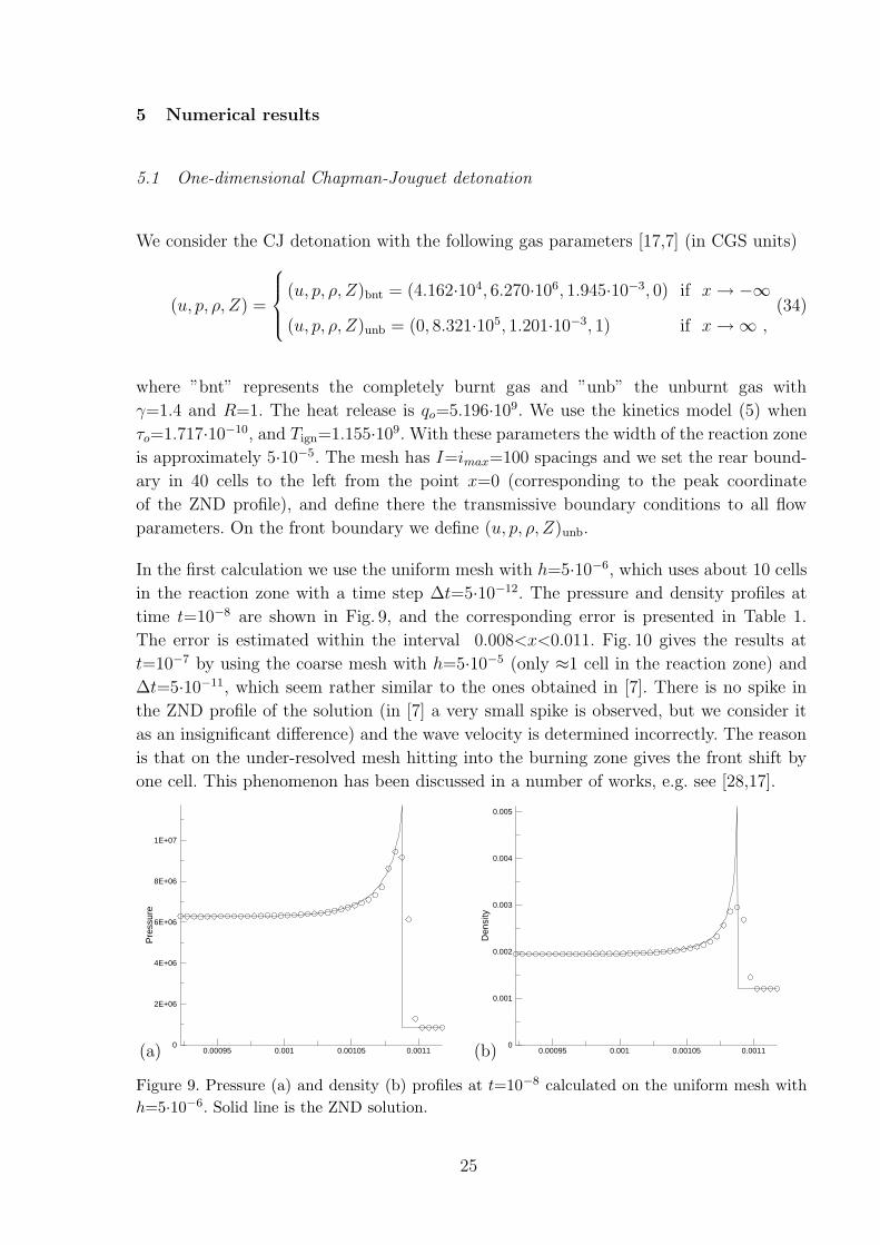
In the first calculation we use the uniform mesh with h=5·10−6, which uses about 10 cells

in the reaction zone with a time step ∆t=5·10−12. The pressure and density profiles at

time t=10−8 are shown in Fig. 9, and the corresponding error is presented in Table 1.

The error is estimated within the interval 0.008<x<0.011. Fig. 10 gives the results at

t=10−7 by using the coarse mesh with h=5·10−5 (only ≈1 cell in the reaction zone) and

∆t=5·10−11, which seem rather similar to the ones obtained in [7]. There is no spike in

the ZND profile of the solution (in [7] a very small spike is observed, but we consider it

as an insignificant difference) and the wave velocity is determined incorrectly. The reason

is that on the under-resolved mesh hitting into the burning zone gives the front shift by

one cell. This phenomenon has been discussed in a number of works, e.g. see [28,17].

(a)

Pre

ssur

e

0.00095 0.001 0.00105 0.00110

2E+06

4E+06

6E+06

8E+06

1E+07

(b)

Den

sity

0.00095 0.001 0.00105 0.00110

0.001

0.002

0.003

0.004

0.005

Figure 9. Pressure (a) and density (b) profiles at t=10−8 calculated on the uniform mesh with

h=5·10−6. Solid line is the ZND solution.

25

(a)

Pre

ssur

e

0.0095 0.01 0.0105 0.0110

2E+06

4E+06

6E+06

8E+06

1E+07

(b)

Den

sity

0.0095 0.01 0.0105 0.0110

0.001

0.002

0.003

0.004

0.005

Figure 10. Pressure (a) and density (b) profiles at t=10−7 calculated on the uniform mesh with

h=5·10−5.

(a)

Pre

ssur

e

0.0009 0.001 0.0011 0.00120

2E+06

4E+06

6E+06

8E+06

1E+07

(b)

Den

sity

0.0009 0.001 0.0011 0.00120

0.001

0.002

0.003

0.004

0.005

Figure 11. Pressure (a) and density (b) profiles at t=10−8 calculated on the adapted mesh with

initial spacing h=5·10−5 as in Fig. 10.

Next, we perform calculations on the adapted mesh. We start on the same coarse uniform

mesh with h=5·10−5 and piece-wise initial data (34). After achieving the steady state, this

solution and its induced adapted mesh are used as initial data for the adaptive modeling.

Otherwise we would obtain an incorrect DCJ velocity. The results are presented in Fig. 11

and Table 1. The mass fraction Z is used as the control function f . Here at every time

step we perform 20 mesh iterations, the coefficient of adaptation used is ca=0.7, and the

iterative parameter in (31) is τ=0.4. It is seen from Fig. 11 that the spike profile is better

resolved than that of in Fig. 9 since after the mesh adaptation the minimal spacing in

the reaction zone is hmin=1.56·10−6 which is about 3.2 times smaller than the uniform

mesh spacing in Fig. 9. Thus, the spacing in the critical zone is decreased by a factor of 32

relative to the initial mesh. Note that the time step decreases approximately by a factor of

32 as well that follows from (14). In fact the effective reduction of h is about 45, because

ahead the detonation wave (already over 2 cells) the spacing is h≈7.1·10−5 and behind the

burning zone h≈2.5·10−5. Despite these facts the error to the adapted solution is slightly

larger than that to the uniform mesh solution with h=5·10−6, as observed in Table 1.

26

This is due to the lack of nodes in the smooth part of the reaction zone. Nevertheless,

due to adaptation, on the coarse mesh we obtained nearly the same accuracy as that of

on the refined one. It is of interest to see that from the side of the heating shock the

mesh is sharply condensed, within one cell the spacing is reduced by several tenths of

times. In this manner the mesh is condensed for the non-reactive gas flow problems with

shock waves [4]. From the side of the burnt gas, where the solution is smooth, the nodes

concentrate gradually. For the smooth solution as ca→∞ we get the optimal grid in the

sense that the error in the norm L∞ on such a mesh is minimal [3].

Table 1

Numerical error for the pressure and density relative to ZND solution.

||Er(p)||L1||Er(ρ)||L1

Unifrom mesh, h=5·10−6 1.22·102 3.28·10−8

Adapted mesh, hmin=1.56·10−6 1.37·102 4.00·10−8

5.2 Unstable one-dimensional detonation

First experiments and then a theoretical analysis, see [23,37], have shown that overdriven

detonation may be unstable in a gas for some range of the parameters. Now we calculate

one such a case of the unstable detonation for the Arrhenius kinetics model (4). The

dimensionless parameters by reference to the uniform state ahead the detonation shock,

moving to the right, are γ=1.2, qo=50, E+=50, the degree of overdrive f = (D/DCJ)2=1.6,

where D is the shock speed, Ko=230.75, R=1, (u, p, ρ, Z)unb=(0, 1, 1, 1). This problem was

also simulated numerically in [25,8,44,42,29].

We conduct calculations in two ways: first, on the fixed mesh, and, second, with shock

tracking on the moving mesh. In both cases the spacing h is equal 0.05, which corresponds

to having 20 cells per half-reaction length for the ZND profile (20 pts/L1/2), which is used

as initial data. At the rear boundary we define the piston velocity as that of for the ZND

profile, i.e. set u=ubnt, and the transmissive boundary conditions for p, ρ, Z. On the front

boundary we define (u, p, ρ, Z)unb.

In the first case of the fixed mesh simulation we set ccfl=0.5. The modeling is performed in

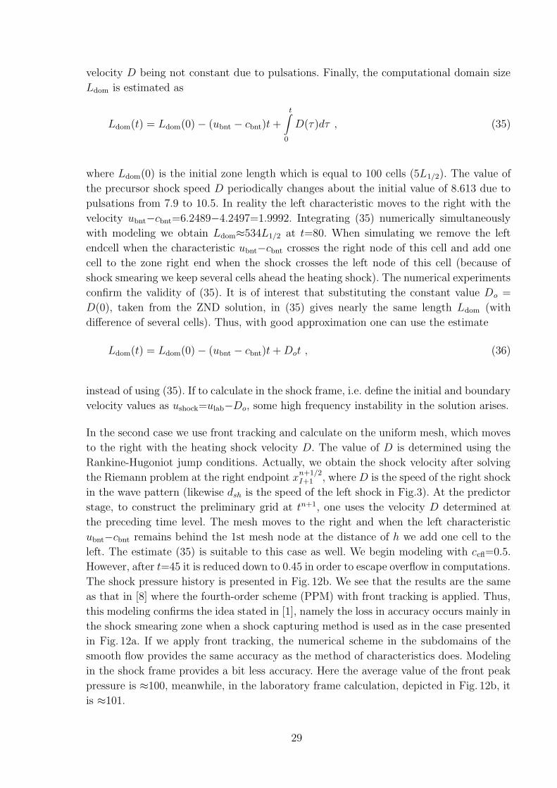
the laboratory frame. The shock pressure history is depicted in Fig. 12a. For comparison,

the result obtained in [8] using the piecewise parabolic method (PPM) with shock fitting

on the fixed mesh is also depicted. We observe a good agreement in the amplitude (the

difference of peak pressure ≤ 3%) and in the wave velocity.

Consider the length of the computational domain which we should retain behind the

shock during modeling. By theory, see [58], the steady overcompressed detonation mode

is possible if the formation of the rarefaction wave is not allowed after the burning process

is ended. Therefore, one needs to move the piston with the medium velocity ubnt at point

27

(a)

x

x

x

x

x

x

x

x

x

x

x

x

x

x

x

x

x

x

x

x

x

x

Time

Sho

ckP

ress

ure

0 10 20 30 40 50 60 70 8050

60

70

80

90

100

(b)

x

x

x

x

x

x

x

x

x

x

x

x

x

x

x

x

x

x

x

x

x

x

Time

Sho

ckP

ress

ure

0 10 20 30 40 50 60 70 8050

60

70

80

90

100

Figure 12. Peak pressure history for unsteady flow. Symbol ”x” indicates the solution in [8], solid

line is the present results. Calculation on the fixed mesh (a). Calculation with front tracking on

the mesh moving with the shock speed D (b).

5 in Fig. 1 to support the overdriven detonation, which can not occur in the free mode

without support. This value can be corrupted due to the disturbances moving from the flow

domain to the burning zone left end with the speed of ubnt − cbnt, where cbnt is the sound

speed in the burnt gas. It is the left characteristic motion that defines the computational

domain length. In addition, the zone right endpoint moves to the right with the shock

28

velocity D being not constant due to pulsations. Finally, the computational domain size

Ldom is estimated as

Ldom(t) = Ldom(0) − (ubnt − cbnt)t +

t∫

0

D(τ)dτ , (35)

where Ldom(0) is the initial zone length which is equal to 100 cells (5L1/2). The value of

the precursor shock speed D periodically changes about the initial value of 8.613 due to

pulsations from 7.9 to 10.5. In reality the left characteristic moves to the right with the

velocity ubnt−cbnt=6.2489−4.2497=1.9992. Integrating (35) numerically simultaneously

with modeling we obtain Ldom≈534L1/2 at t=80. When simulating we remove the left

endcell when the characteristic ubnt−cbnt crosses the right node of this cell and add one

cell to the zone right end when the shock crosses the left node of this cell (because of

shock smearing we keep several cells ahead the heating shock). The numerical experiments

confirm the validity of (35). It is of interest that substituting the constant value Do =

D(0), taken from the ZND solution, in (35) gives nearly the same length Ldom (with

difference of several cells). Thus, with good approximation one can use the estimate

Ldom(t) = Ldom(0) − (ubnt − cbnt)t + Dot , (36)

instead of using (35). If to calculate in the shock frame, i.e. define the initial and boundary

velocity values as ushock=ulab−Do, some high frequency instability in the solution arises.

In the second case we use front tracking and calculate on the uniform mesh, which moves

to the right with the heating shock velocity D. The value of D is determined using the

Rankine-Hugoniot jump conditions. Actually, we obtain the shock velocity after solving

the Riemann problem at the right endpoint xn+1/2I+1 , where D is the speed of the right shock

in the wave pattern (likewise dsh is the speed of the left shock in Fig.3). At the predictor

stage, to construct the preliminary grid at tn+1, one uses the velocity D determined at

the preceding time level. The mesh moves to the right and when the left characteristic

ubnt−cbnt remains behind the 1st mesh node at the distance of h we add one cell to the

left. The estimate (35) is suitable to this case as well. We begin modeling with ccfl=0.5.

However, after t=45 it is reduced down to 0.45 in order to escape overflow in computations.

The shock pressure history is presented in Fig. 12b. We see that the results are the same

as that in [8] where the fourth-order scheme (PPM) with front tracking is applied. Thus,

this modeling confirms the idea stated in [1], namely the loss in accuracy occurs mainly in

the shock smearing zone when a shock capturing method is used as in the case presented

in Fig. 12a. If we apply front tracking, the numerical scheme in the subdomains of the

smooth flow provides the same accuracy as the method of characteristics does. Modeling

in the shock frame provides a bit less accuracy. Here the average value of the front peak

pressure is ≈100, meanwhile, in the laboratory frame calculation, depicted in Fig. 12b, it

is ≈101.

29

It may be of interest to note that the admissible time step ∆t in the moving mesh cal-

culation is substantially larger than that of on the fixed mesh. In fact, if we perform

estimation of ∆t at t=0, from (14) in the left endcell, where

drght1 = ubnt + cbnt = 10.499 , dlft

2 = ubnt − cbnt = 1.9992 , w1 = w2 = D = 8.613

we obtain

∆t3/2 =h

max(drght1 − w2 , −dlft

2 + w1)= 7.55·10−3 .

Meanwhile on the fixed mesh, where wi=0, we have ∆t3/2 = 4.76·10−3.

In the right Ith cell, immediately behind the shock, with the values obtained from

the Riemann problem on the moving mesh drghtI =10.626 and dlft

I+1=4.782, we have

∆tI+1/2=1.31·10−2 . On the fixed mesh with drghtI =10.635 , dlft

I+1=4.76 the time step is

∆tI+1/2=4.70·10−3. Thus, the time steps ratio grows from 1.59 in the left endcell to 2.78

in the right endcell. This is due to the left characteristic moves in the same direction as

the grid nodes on the moving mesh. Indeed, by (13) we should use the minimal step and

multiply it by ccfl. Finally, by t=80 we perform 35597 time steps on the fixed mesh and

23488 steps on the moving mesh.

5.3 Unstable two-dimensional detonation

As in one-dimensional case the planar flow is also unstable in a range of the flow para-

meters, e.g. see [48,49]. The theory of this phenomena, giving rather qualitative sketch,

can be found e.g. in [26]. The structure of the two-dimensional flow is rather complicated.

Thus, a precise numerical simulation is of interest.

We present the results of modeling the unstable detonation in a channel drawn in

[9,44], when the transversed waves (or cellular structure) are produced. The gas with

degree of overdrive f=1.2 flows in the channel with the height equal 10L1/2. We use

the kinetics model (4) with dimensionless parameters γ=1.2, qo=50, E+=10, Ko=3.124,

(u, v, p, ρ, Z)unb=(0, 0, 1, 1, 1). The ZND profile is used as initial data. On the top and

bottom of the channel the periodic boundary conditions are applied. On the rear bound-

ary we define the piston velocity u=ubnt, and transmissive boundary conditions for the

other parameters. The rectangular mesh is hx=hy=h=0.05, i.e. 20 pts/L1/2. The planar

detonation front is disturbed allowing it within the first 103 time steps to ingest a small

region of fluid (5 cells in width and 100 in height) with the rate constant K ′o=0.8Ko.

The question of interest is how far should we place the rear boundary, i.e. piston. The

fact is that we perform calculations up to time t≈62 and, therefore, with the steady

ZND’s mode values Do=7.459, ubnt=4.704, cbnt=4.0 and initial Ldom(0)=5L1/2 via (36)

30

one estimates the length of 424L1/2 or 8480 cells to be used in the end. It is not realistic

to calculate on such a mesh. To overcome this difficulty, we performed the following

numerical experiment. First, it was conducted three calculations on the rough mesh with

h=0.2 till time t=40 when the flow structure is developed. In the first case we calculate

throghout the domain of Ldom≈275L1/2 (1375 cells) determined via (36). In the second

case we set Ldom=60L1/2 (300 cells), and in the third case Ldom=40L1/2 (200 cells). By

the reason stated in section 5.2 we calculate in the laboratory frame and keep eliminating

cells at the left end and adding cells ahead the shock front. The difference of the maximal

peak pressures for the 1st and 2nd cases at t=40 is less than 0.01%, and for the 1st and

3rd cases is less than 1%. We believe that for our calculations on the refined mesh it is

sufficient to keep the rear boundary at the distance of 40L1/2 behind the detonation wave

front. Thus, the problem is computed on the 800×200 mesh. In all calculations the CFL

number is ccfl=0.5.

First, the calculation is executed on the rectangular mesh. For t=60 the running time

on PC Pentium 2.0 GHz is about 36 hours. Fig. 13 shows the pressure contours from

t = 60.060 to 62.735 (see also Figs. 17a, 19a). The general structure of the solution is

similar to that in [9,44].

The moving mesh calculation is executed in two ways. In the first, the front tracking

procedure, described in sec. 3.4, is employed. Here the right edges of the right row cells

are the precursor shock front. At every time step, after the wave front has been shifted,

the functional (32) is employed to redistribute the boundary nodes and (27) to move the

internal nodes. In addition we can switch on the adaptive procedure, see examples of

the meshes in Fig. 14. In the second case we apply the global adaptation without front

tracking, see the meshes in Figs. 16,18.

When adapting, as a control function f it is used the density, see mesh in Fig. 14a, and

pressure, Figs. 14b,16,18. The choice of f is defined by what traits of the flow pattern to

be investigated in detail. The parameter Dmax in (30) is set from 10 to 15. At every time

step we perform 2 mesh iterations (therefore, update the gas dynamics parameters three

times), and set τ=0.9 in (29), coefficient ca is set from 0.07 to 0.1. When adapting, at

first mesh iteration the initial mesh at tn+1 is determined by the formulas

xn+1i,j = xn

i,j + Do4t , yn+1i,j = yn

i,j .

Using adaptation we aim to resolve as much as possible the main (i.e. most intensive)

singularities in the solution and by this reason we condense strongly the grid lines. Ad-

missible time step ∆t falls from 1.5·10−3 on the rectangular mesh by 5 to 10 orders of

magnitude, i.e. practically goes to zero. Note that ∆t is not a constant even for the steady

problems, the mesh constantly ”breaths”, and, accordingly, the value of ∆t periodically

decreases and then increases, etc. Indeed, we can not calculate within a long period of

the ”flow” time with such an infinitesimal ∆t. Thus, we can operate in two ways: first,

31

starting the adaptation when necessary from the initial state, obtained on the rectangular

mesh, or, second, weakening adaptation by reducing the coefficient of adaptation ca and,

therefore, increasing ∆t.

Further we will be concern with some particular features of the flow pattern and compare

the results of the fixed and moving mesh calculations. The density plots for the rectangular

mesh modeling at t=60.44 are depicted in Fig. 15a. The flow structure behind the Mach

stem, inside the cell, is rather unclear due to the presence of oscillations. We can not

observe neither how close the fire zone approaches the precursor shock nor the slip lines

emanating from the upper and lower triple points. Results of front tracking, see Fig. 15b,

show the front part of the fire zone and slip lines impinging on it. It is of interest that

the form and location of the fire zone differs from qualitative results predicted in [26]. In

[26], the fire zone lays immediately behind the Mach stem and is parallel, meanwhile in

Fig. 15b it bends strongly. Evidence that it is the fire zone one can find in Fig. 15d with the

mass fraction plots depicted. The fire zone has no a structure behind the incident shock.

Among all flow parameters the density plots have the most complicated structure, which

can be better seen in Fig. 15c of the adaptive mesh calculation. Indeed, we can not resolve

all the solution traits by grid lines condensing, but the main discontinuities are reflected

in the mesh structure rather well, see Fig. 14a. Meanwhile the density ”feels” the fire zone

and a bit slip lines, see Fig. 14a, using the pressure as f gives a better resolution of the

transverse waves, both intensive and weak, emanating from the triple points and beginning

to emerge behind the incident shock, see the meshes in Figs.14b,16,18. Capturing the slip

lines by grid lines condensing is not subject to an instability, as may be expected. As shown

in [4] for the example of the contact discontinuity in the one-dimensional linear model,

our adaptive method can not prevent slip lines smearing with time. Besides, the ”barrier”

property of this grid generator prevents the mesh cells from infinitesimal refinement [14,4],

which is regulated by the coefficient ca value.

Between two transverse shocks, depicted in Fig. 16b (one intensive and the other weak),

the grid cell size changes sharply in the normal direction to those shocks. It seems possible

that the approximation on such a mesh is to deteriorate. However, first, as shown in [4], a

large ratio of the neighboring cells size (one in the smeared-out shock zone and the other

in the domain of smooth flow), does not deteriorate the solution. Second, the narrow cells

in the shock zone lead the scheme, based on the integral conservation laws, to update

the flow parameters nearly as the shock fitting procedure via the Rankine-Hugoniot jump

conditions [4]. This conclusion can be drawn from the following consideration. If to draw

a closed contour along the shock, one side to the left of the discontinuity and the other

to the right, and to direct the contour width to zero, from the system of conservation

laws, written in the integral form, in the limit we get the Rankine-Hugoniot jump con-

ditions [46,31]. The imaginarily drawn line, passing through the centers of narrow cells

in the shock zone, looks like that contour when the width-to-length cell ratio tends to

zero. Thus, due to adaptation, the flow solver, by grid cell size variation, is adjusted to

perform the habitual calculations in the domains of smooth flow and to operate as the

32

front fitting procedure in the shock zone. The experimental evidence of this statement

can be seen by comparing the pressure contours obtained on the rectangular and adapted

meshes. Oscillations in pressure behind the precursor shock, observed in Fig. 17a, disap-

pear in Fig. 17d. In this regard the global adaptation, Fig. 17d, works like front tracking,

Fig. 17b,c. Note that with front tracking one can only treat the precursor shock (and

it is a special procedure), meanwhile the global adaptation operates with the ”intensive

singularities” throughout the flow automatically.

The fragment of the mesh near the top boundary is shown in Fig. 16c. If the constrained

minimization is not used to the boundary nodes redistribution, we can not obtain such a

fine-mesh structure. Numerical experiments have shown that instability in the adaptive

mesh generation on the boundary (if no constrained minimization) leads to interior domain

instability, rather far from the boundary.

6 Concluding remarks

In this work, the unsplit scheme to model the reactive gas flow on the moving meshes has

been presented. This scheme allows for calculations coupled with front tracking, which

enhance the accuracy of simulation. Using the moving adaptive meshes allows us to con-

centrate locally the grid points in the vicinity of singularities: shocks, slip lines, rarefaction

waves, and fire zones, while keeping the simple mesh structure and invariable number of

nodes. Numerical experiments have shown that using adaptive meshes allows efficiently

resolving the thin structures of the solution. Strongly condensed grid lines in the vicin-

ity of shocks lead the flow solver is adjusted to perform calculations like using the jump

conditions and this, in turn, gives significant accuracy enhancement of the modeling.

In the 3D calculations, some principal difficulties in mesh generation still need to be

overcome. First, it concerns with the search of a transformation providing a homeomorphic

mapping of the unit cube onto an arbitrary domain in the continuous approach. Note that

in the 3D case it is unknown yet whether a harmonic mapping of an arbitrary domain onto

a convex domain (unit cube) with a given one-to-one mapping between the boundaries is

always a homeomorphism. There is an example (see [24]), when, subject to some conditions

imposed on the boundaries, the harmonic mapping is not a homeomorphism. Second,

for a hexahedral cell there unknown a finite number of conditions using which one can

definitely say whether this cell is invertible or not [54]. One of possible ways to overcome

these difficulties is to seek directly a discrete mapping. One such example was considered

in [34]. Anyway, an additional thorough study is required to execute in this direction.

33

Acknowledgments

The work of B.N. Azarenok was partially supported by Russian Fund of Fundamental Re-

search (project code 02-01-00236). The work of T. Tang was partially supported by Hong

Kong Research Grant Council (Project Code HKBU2045/02P and HKBU 2018/03P) and

International Research Team on Complex System, Chinese Academy of Sciences.

References

[1] G.B. Alalykin, S.K. Godunov (Ed.), I.L. Kireeva, and L.A. Pliner, Solution of One-

Dimensional Problems in Gas Dynamics on Moving Meshes, Nauka Press (Moscow, 1970).

[2] B.N. Azarenok, Realization of a second-order Godunov’s scheme, Comp. Meth. in Appl.

Mech. and Engin., 189 (2000), pp. 1031–1052.

[3] B.N. Azarenok and S.A. Ivanenko, Application of moving adaptive grids for numerical

solution of nonstationary problems in gas dynamics, Int. J. for Numer. Meth. in Fluids,

39 (2002), No. 1, pp. 1–22.

[4] B.N. Azarenok, Variational barrier method of adaptive grid generation in hyperbolic

problems of gas dynamics. SIAM J. Numer. Anal., 40 (2002), No. 2, pp. 651–682.

[5] B.N. Azarenok, S.A. Ivanenko, and T. Tang, Adaptive mesh redistribution method based

on Godunov’s scheme, Comm. Math. Sci., 1 (2003), No. 1, pp. 152–179.

[6] W. Bao and S. Jin, The random projection method for hyperbolic systems with stiff reaction

terms, J. Comput. Phys., 163 (2000), pp. 216–248.

[7] M. Ben-Artzi, The generalized Riemann problem for reactive flows, J. Comput. Phys., 81

(1989), pp. 70–101.

[8] A. Bourlioux, A.J. Majda, and V. Roytburd, Theoretical and numerical structure for

unstable one-dimensional detonations, SIAM J. Appl. Math., 51, 1991, No. 2, pp. 303–

343.

[9] A. Bourlioux, A.J. Majda, Theoretical and numerical structure for unstable two-

dimensional detonations, Combustion and Flame, 90 (1992), pp. 211–229.

[10] J.U. Brackbill and J.S. Saltzman, Adaptive zoning for singular problems in two dimensions,

J. Comput. Phys., 46 (1982), pp. 342–368.

[11] W.M. Cao, W.Z. Huang, and R.D. Russel, An r-adaptive finite element method based upon

moving mesh PDEs, J. Comput. Phys. 149 (1999), pp. 221–244.

[12] J. Casper and M.H. Carpenter, Computational considerations for the simulation of shock-

induced sound, SIAM J. Sci. Comp., 19 (1998), No. 3, pp. 813–828.

34

[13] A.A. Charakhch’yan and S.A. Ivanenko, Curvilinear grids of convex quadrilaterals, USSR

Comput. Math. Math. Phys. 28 (1988), No. 2, pp. 126–133.

[14] A.A. Charakhch’yan and S.A. Ivanenko, A variational form of the Winslow grid generator,

J. Comput. Phys., 136 (1997), pp. 385–398.

[15] V.A. Cherkashin, A.V. Zabrodin, Method of numerical modeling the detonation wave,

Keldysh Institute of Applied Mathematics, USSR Academy of Sciences, Internal report

(1974).

[16] A.J. Chorin, Random choice solution of hyperbolic systems, J. Comput. Phys., 22 (1976),

pp. 517–531.

[17] P. Colella, A. Majda, and V. Roytburd, Theoretical and numerical structure for reacting

shock waves, SIAM J. Sci. Statist. Comput., 7 (1986), pp. 1059–1080.

[18] R. Courant and K.O. Friedrichs, Supersonic Flow and Shock Waves, Springer-Verlag

(1985).

[19] M. G. Crandall and A. Majda, The method of fractional steps for conservation laws, Numer.

Math., 34 (1980), pp. 285–314.

[20] Yu.N. Deryugin, V.P. Kopyshev, and B.P. Tikhomirov, On detonation calculation by Forest

Fire model using Godunov’s method, Questions of Atomic Science and Technique, 1 (1990),

pp. 48–52.

[21] A.S. Dvinsky, Adaptive grid generation from harmonic maps on Riemannian manifolds, J.

Comput. Phys., 95 (1991), pp. 450–476.

[22] B. Engquist and B. Sjogreen, The convergence rate of finite difference schemes in the

presence of shocks, SIAM J. Numer. Anal., 35 (1998), No. 6, pp. 2464–2485.

[23] J.J. Erpenbeck, Stability of idealized one-reaction detonations, Phys. Fluids, 7 (1964), pp.

684–696.

[24] F.T. Farrell and L.E. Jones, Some non-homeomorphic harmonic homotopy equivalences.

Bull. London Math. Soc., 28, 1996, pp. 177–182.

[25] W. Fickett and W.W. Wood, Flow calculations for pulsating one-dimensional detinations,

Phys. Fluids, 9 (1966), pp. 903–916.

[26] W. Fickett and W.C. Davis, Detonation, University of California Press, (Berkeley, CA,

1979).

[27] V.E. Fortov, B. Goel, C.D. Munz, A.L. Ni, A.V. Shutov, and O.Yu. Vorobiev, Numerical

simulation of Nonstationary Fronts and Interfaces by the Godunov Method in Moving

Grids, Nuclear Science and Engineering , 123 (1996), pp. 169–189.

[28] C. Helzel, R.J. LeVeque, and G. Warneke, A modified fractional step method for the

accurate approximation of detonation waves, SIAM J. Sci. Comput., 22, No. 4 (2000), pp.

1489–1510.

35

[29] P. Hwang, R. Fedkiw, B. Merriman, A.R. Karagozian, and S.J. Osher, Numerical resolution

of pulsating detonation waves, Combustion Theory and Modeling , 4, (2000), No. 3, pp. 217–

240.

[30] S.K. Godunov and G.P. Prokopov, On computation of conformal transformations and

construction of difference meshes, Zh. Vychisl. Mat. Mat. Fiz., 7 (1967), pp. 1031–1059.

[31] S.K. Godunov (Ed.), A.V. Zabrodin, M.Ya. Ivanov, A.N. Kraiko, and G.P.

Prokopov, Numerical Solution of Multi-Dimensional Problems in Gas Dynamics, Nauka

Press (Moscow, 1976); (French translation: Resolution Numerique des Problemes

Multidimensionnels de la Dynamique des Gaz, Mir, Moscou, 1979.)

[32] S.K. Godunov, Equations of Mathematical Physics, Nauka Press (Moscow, 1979).

[33] S.K. Godunov, Reminiscenses about difference schemes, J. Comput.Phys., 153 (1999), pp.

6–25.

[34] Ivanenko S.A. Harmonic Mappings, Chapt. 8 in Handbook of Grid Generation. CRC Press,

Boca Raton, Fl, 1999.

[35] O.B. Khairullina, A.F. Sidorov, O.V. Ushakova, Variational methods of Construction of

optimal grids, Chapt. 36 in: Handbook of Grid Generation, J.F. Thompson et al. eds., CRC

Press, Fl, (1999).

[36] A.G. Kulikovskii, N.V. Pogorelov, and A.Yu. Semenov, Mathematical Aspects of

Numerical Solution of Hyperbolic Systems, Monographs and Surveys in Pure and Applied

Mathematics, 188, (Chapman and Hall/CRC, Boca Raton, FL, 2001).

[37] H.I. Lee and D.S. Stewart, Calculation of linear detonation instability: one-dimensional

instability of plane detonation, Journal of Fluid Mechanics, 216 (1990), pp. 103–132.

[38] B. van Leer, Towards the ultimate conservative difference scheme. V. A second order sequel

to Godunov’s methods, J. Comput.Phys., 32 (1979), pp. 101–136.

[39] V.D. Liseikin, On generation of regular grids on n-dimensional surfaces, USSR Comput.

Maths. Math. Phys., 31 (1991), No. 11, pp. 47–57.

[40] V.V. Ostapenko, Convergence of Finite-Difference Schemes behind a Shock Front, Comput.

Math. Math. Phys., 37 (1997), No. 10, pp. 1161–1172.

[41] E. Oran and J.P. Boris, Numerical Simulation of Reactive Flow, Elsevier, (New York,

1987).

[42] M.V. Papalexandris, A. Leonard, and P.E. Dimotakis, Unsplit schemes for hyperbolic

conservation laws with source terms in one space dimension, J. Comput.Phys., 134 (1997),

pp. 31–61.

[43] R.B. Pember, Numerical methods for hyperbolic conservation laws with stiff relaxation I.

Spurious solutions, SIAM J. Appl. Math., 53 (1993), pp. 1293–1330.

[44] J.J. Quirk, Godunov-type schemes applied to detonation flows, Combustion in High-Speed

Flows, ed. J. Buckmaster et al, Dordrecht: Kluwer , (1994), pp. 575–596.

36

[45] A.V. Rodionov, Increase of accuracy of Godunov’s scheme, USSR Computational Math.

and Math. Phys., 27, No. 12 (1987), pp. 1853–1860.

[46] B.L. Rozhdestvenskii and N.N. Yanenko, Systems of Quasilinear Equations and Their

Applications to Gas Dynamics, Amer. Math. Soc. Transl. of Math. Monographs, 55, AMS,

Providence, RI, 1983.

[47] R. Schoen and S. T. Yau, On univalent harmonic maps between surfaces, Invent. Math.,

44 (1978), pp. 265–278.

[48] G.J. Sharpe, Linear stability of idealized detonations, Proc. of Royal Soc. of Lond., Ser.

A, 453 (1997), pp. 2603–2625.

[49] M. Short and D.S. Stewart, Cellular detonation stability, Part 1. A normal-mode linear

analysis, Journal of Fluid Mechanics, 368 (1998), pp. 229–262.

[50] H.Z. Tang ang T. Tang, Adaptive mesh methods for one- and two-dimensional hyperbolic

conservation laws, SIAM J. Numer. Anal., 41 (2003), pp. 487–515.

[51] T. Tang and Z.-H. Teng, Error bounds for fractional step methods for conservation laws

with source terms, SIAM J. Numer. Anal., 32 (1995), pp. 110–127.

[52] T. Tang, Convergence analysis for operator splitting methods to conservation laws with

stiff source terms, SIAM J. Numer. Anal., 35 (1998), pp. 1939–1968.

[53] V.T. Ton, Improved shock-capturing methods for multicomponent and reacting flows, J.

Comput. Phys., 128 (1996), pp. 237–253.

[54] Ushakova O.V. Conditions of nondegeneracy of three-dimensional cells. A formula of a

volume of cells, SIAM J. Sci. Comp, 23 (2001), No. 4, pp. 1273–1289.

[55] N.N. Yanenko, N.T. Danaev, and V.D. Liseikin, On variational method to cunstructing

meshes, Chislen. Metody Mekhan. Sploshn. Sredy , 8, No. 4 (1977), Novosibirsk, pp. 157–

163.

[56] H. Weyl, Shock waves in arbitrary fluids, Comm. Pure Appl. Math., 2, No. 2–3 (1949), pp.

103-122.

[57] A. Winslow, Numerical solution of the quasi-linear Poisson equation in a nonuniform

triangle mesh, J. Comput. Phys., 1 (1966), pp. 149–172.

[58] Ya.B. Zeldovich and S.A.Kompaneets, Theoriya Detonatsii (Theory of Detonations),

Gostekhizdat (Moscow, 1955) (English translation: Academic Press , New York, 1960.)

37

(a) (d)

(b) (e)

(c) (f)

Figure 13. Pressure contours at t=60.060 (a), 60.824 (b), 61.205 (c), 61.981 (d), 62.362 (e),

62.735 (f) for rectangular 800×200 mesh calculation. Only 250 cells in the x-direction near the

wave front are presented.

38

(a) (b)

Figure 14. Front tracking and adaptation. Meshes at t=60.44 with density (a) or pressure (b)

as a control function f . Only 60 front cells in the x-direction are depicted.

39

(a) (b)

(c) (d)

Figure 15. Density plots at t=60.44 for rectangular mesh (a), front tracking (b), front tracking

with adaptation (c) (mesh in Fig.14a) calculation. Mass fraction for front tracking calculation

(d).

40

(a)

(b) (c)

Figure 16. Global adaptation with p as a control function f . Mesh (a) and close-up (b,c) at

t=60.44; time step ∆t=10−10−10−5·∆trect.

41

(a) (b)

(c) (d)

Figure 17. Pressure plots at t=60.44 for rectangular mesh (a), front tracking (b), front tracking

with adaptation (c) (mesh in Fig.14b), and global adaptaion (d) (mesh in Fig.16) calculation.

42

(a)

(b)

Figure 18. Global adaptation with p as a control function f . Mesh (a) and close-up (b) at

t=61.59.43

(a) (b)

(c) (d)

Figure 19. Pressure plots at t=61.59 computed on the rectangular (a) and adapted (b) mesh.

Close-up for the rectangular (c) and adapted (d) mesh (domain, depicted in Fig 18b).

44