Second-Order Induction: Uniqueness and

Complexity∗

Rossella Argenziano† and Itzhak Gilboa‡

August 2018

Abstract

Agents make predictions based on similar past cases, while also learning the

relative importance of various attributes in judging similarity. We ask whether

the resulting “empirical similarity” is unique, and how easy it is to find it.

We show that with many observations and few relevant variables, uniqueness

holds. By contrast, when there are many variables relative to observations,

non-uniqueness is the rule, and finding the best similarity function is computa-

tionally hard. The results are interpreted as providing conditions under which

rational agents who have access to the same observations are likely to con-

verge on the same predictions, and conditions under which they may entertain

different probabilistic beliefs.

Keywords: Empirical Similarity, Belief Formation.

∗We thank Yotam Alexander, Thibault Gajdos, Ed Green, Offer Lieberman, Yishay Mansour,and David Schmeidler for comments and references. Gilboa gratefully acknowledges ISF Grant704/15.†Department of Economics, University of Essex. r.argenziano@essex.ac.uk‡HEC, Paris, and Tel-Aviv University. tzachigilboa@gmail.com

1

1 Introduction

Where do beliefs come from? How do, and how should economic agents estimate

the likelihood of future events? Decision theory remains mostly silent on this point.

The axiomatic foundations laid by Ramsey (1926a,b), de Finetti (1931,1937), Savage

(1954), and Anscombe-Aumann (1963) are very powerful in arguing that rational

individuals should behave as if they had probabilistic beliefs (to be used for expected

utility maximization), and arguably also that actual economic agents behave this way.

But they shed no light over the question of the selection of prior probabilities. In a

sense, they deal with form but not with content.

The natural answer to the belief formation problem is provided by equilibrium

analysis: whether in games or in markets, rational agents’ beliefs are assumed to

coincide with the modeler’s. However, equilibria need not be unique. And, more

fundamentally, one needs to ask whether agents’behavior will converge to an equi-

librium in the first place, which brings us back to the belief formation question. In

short, it appears that there is a need for theories of belief formation that would be

(i) relatively general and applicable to a variety of economic settings; (ii) suffi ciently

rational to credibly apply to weighty economic decisions; and (iii) intuitive enough to

be thought of as idealized models of the way actual people think.

In the quest for reasonable models of belief formation, two fellow disciplines might

be of help: statistics and psychology. The former has a normative flavor, while

the latter —descriptive. Statistics and, more recently, machine learning attempt to

develop effective ways of prediction based on past data, with no claim to describe the

way people think. By contrast, psychology aims at modeling human reasoning, be it

more or less rational. Recent developments in cognitive science highlight a promising

bridge between these disciplines: a specific class of learning techniques developed in

statistics and machine learning, namely kernel methods and support vector machines,

are closely related to ‘exemplar learning’ models developed in psychology: “...kernel

methods have neural and psychological plausibility, and theoretical results concerning

their behavior are therefore potentially relevant for human category learning.”(Jaekel,

Schoelkopf, and Wichmann, 2009, p. 381). This paper presents a model of belief

formation based both on kernel techniques and on insights from the exemplar learning

literature.

We start by assuming that the probability of a future event is estimated by its

2

similarity-weighted relative frequency in the past.1 More explicitly, given past obser-

vations (xi, yi)i≤n (where xi is a vector of real-valued predictors and yi is the indicator

of the event in question), and a new point xp, the probability of the event occurring

next is estimated by

P (yp = 1) =

∑i≤n s(xi, xp)yi∑i≤n s(xi, xp)

(1)

where s is a non-negative similarity function defined on pairs of x vectors. When

all past events are deemed equally relevant, probability is estimated by empirical

frequency. But in general past occurrences are weighted by their similarity: more

similar circumstances gain higher weight than less similar ones. This estimation is

referred to as first-order induction.

The second level of learning involves finding a similarity function, to be used in

(1), from the data as well. Specifically, we consider a Leave-One-Out cross-validation

technique: each similarity function is assessed by the sum of squared errors it would

have yielded, were it to be used in sample, to predict each yi based on the other

observations. A function that brings this sum of squared errors to a minimum is

referred to as an “empirical similarity”, and it is used here as an obviously idealized

model of the way people learn which features are more important than others to assess

similarities. Because this process deals with learning how first-order induction should

be performed, it will be dubbed second-order induction.

We first point out that the empirical similarity function need not take into ac-

count all the variables available. For reasons that have to do both with the curse of

dimensionality and with overfitting, one may prefer to use a relatively small set of the

variables to a superset thereof. We provide conditions under which it is worthwhile

to add a variable to the arguments of the similarity function. Next, we observe that

the empirical similarity need not be unique, and that people who have access to the

same database may end up using different similarity functions to obtain the “best”

fit. Further, we show that finding the best similarity function is a computationally

complex (NP-Hard) problem. Thus, even if the empirical similarity is unique, it does

not immediately follow that all agents can find it. Rational agents might therefore

end up using different, suboptimal similarity functions.

There are many modeling choices to be made, in terms of the nature of the vari-

1We follow the convention in psychology and decision theory to label kernel functions as ‘similarityfunctions.’

3

ables (the predictors and the predicted), as well as of the similarity function. We

study here two extreme cases: in the “binary”model all the variables take only the

values {0, 1}, and so does the similarity function. Further, we consider only similar-ity functions that are defined by weights in {0, 1}: each variable is either taken intoaccount or not, and two observations are similar (to degree 1) if and only if they are

equal on all the relevant variables. In the “continuous”model, by contrast, all vari-

ables (predictors and predicted) are continuous, and the similarity function is allowed

to take any non-negative value as well. We focus on functions that are exponential

in weighted Euclidean distances where the weights are allowed to be non-negative

extended real numbers.

In both models we find the same qualitative conclusions: (i) If the number of

predictors is fixed, and the predicted variable is a function of the predictors, then, as

the number of observations grows following an i.i.d. process, the empirical similarity

will learn the functional relationship. The similarity function is likely to be unique,

but even if it is not, different empirical similarity functions would provide the same

predictions (Propositions 2 and 4). By contrast (ii) If the number of predictors is

large relative to the number of observations, it is highly probable that the empirical

similarity will not be unique (Propositions 3 and 5). Further, (iii) If the number of

predictors is not bounded, the problem of finding the empirical similarity is NPC

(Theorems 1 and 2).

To see the implications of these results, let us contrast two prediction problems:

in the first, an agent tries to estimate the probability of his car being stolen. In

the second, the probability of success of a revolution attempt. In the first problem,

there are several relevant variables to take into account, such as the car’s worth, the

neighborhood in which it is parked, and so forth. One can think of the number of

these variables as relatively limited. By contrast, the number of observations of cars

that were or were not stolen is very large. In this type of problems it stands to reason

that empirical similarity be unique. Further, as the number of variables isn’t large,

the complexity result has little bite. Thus, different people are likely to come up with

the same similarity functions, and therefore with the same probabilistic predictions.

By contrast, in the revolution example the number of observations is very limited.

One cannot gather more data at will, neither by experimentation nor by empirical

research. To complicate things further, the number of variables that might be relevant

predictors may be very large. Researchers may come up with novel perspectives on

4

a given history, and suggest new military, economic, and sociological variables that

might help judge which historical cases are similar to which. In this type of examples

our results suggest that the optimal similarity function may not be unique, and that,

even if it is unique, people may fail to find it. That is, to the extent that second-order

induction describe a psychological process people implicitly go through, they may

learn to judge similarity by functions that are not necessarily the best one. It follows

that they may also not find the same function (even if the “best”one is unique). As a

result, it may not be too surprising that experts may disagree on the best explanation

of historical events, and, consequently, on predictions for the future.

The rest of this paper is organized as follows. The next subsection discusses first-

and second-order induction, and the specific formulas we use, in the literatures in

statistics, psychology, and decision theory. Section 2 deals with the questions of

monotonicity, uniqueness, and computational complexity of the empirical similarity

function in the binary model, while Section 3 provides the counterpart analysis for

the continuous model. Section 4 concludes with a general discussion.

1.1 Related Literature

Using similarity-weighted averages is an intuitive idea that appeared in statistics as

“kernel methods” (Akaike, 1954, Rosenblatt, 1956, Parzen, 1962). Further, it has

also been suggested that the “best” kernel function be estimated from the data.

In particular, Nadaraya (1964) and Watson (1964) suggested to find the optimal

bandwidth of the kernel (see also Park and Marron, 1990). Our focus is mostly on

the qualitative question, namely, which variables to include in the function, rather

than on the quantitative one, that is, how close is “close”. The question of optimal

bandwidth is obviously of interest in applied statistical work, but for the purposes of

economic modeling we find the choice of variables to be of greater import. Be that as

it may, we are unaware of results about optimal kernel functions that are along the

lines of our results here.

Cortes and Vapnik (1995) suggested the widely-used method of “support vector

machines” (SVMs) for classification problems. This technique is based on the idea

that if a simple linear classifier might not exist in the original space, there might

still be one in a higher dimensional space. The latter is often taken to be the kernel

functions defined by points in the learning database, resulting in kernel classification

5

coupled with optimization of the coeffi cients of the kernel function, and of the func-

tions itself. This technique is also used to estimate probabilities (see Vapnik, 2000)

along lines that are similar to logistic regression. We are unaware of results in this

literature that are similar to ours.

The formula (1) also appeared in the psychological literature, in the Generalized

Context Model (Medin and Schaffer, 1978, and Nosofsky, 1984). In this domain the

task that participants in an experiment are asked to perform is typically a classifi-

cation task (to guess whether yp = 1 or yp = 0), rather than probability assessment

(that is, to provide a number in [0, 1] for the probability that yp = 1). However,

when modeling the frequency with which participants classify a new case as yp = 1

or yp = 0, it appears that these frequencies are given by (1). In particular, the model

finds that classification of a new ‘exemplar’ is based on the similarity between the

latter and a set of training exemplars, with a mental process that resembles our notion

of first order induction. Exemplars are represented as points in a multidimensional

psychological space and the similarity between any two is a decreasing function of

their distance in this space (the Multidimensional Scaling Approach, see Shepard,

1957,1987). Importantly, Nosofsky (1988) finds that people seem to learn the relative

importance of different attributes in the similarity function in a process that resem-

bles what we call second order induction. (See Nosofsky, 2014, for a survey). The

fact that, for classification problems, the same formula appeared in machine learning

and in psychology was noted by Jaekel, Schoelkopf, and Wichmann (2008, 2009).

Yet, formal analysis of optimal similarity functions, whether for classification or for

probability estimation, seems to be lacking.

Similarity-based classification was axiomatized in Gilboa and Schmeidler (2003),

and similarity-weighted probability estimation as in (1) was axiomatized in Billot,

Gilboa, Samet, and Schmeidler (2005) and in Gilboa, Lieberman, and Schmeidler,

[GLS] (2006) (the former for the case of y being a discrete variable with at least 3

values, the latter for the case of two values discussed here). GLS (2006) also suggested

the notion of “empirical similarity”, based on the notion of a maximum likelihood

estimator of the similarity, assuming that the actual Data Generating Process (DGP)

is similarity-based.2 Lieberman (2010, 2012) analyzed the asymptotic properties of

2The learning process presented here has been suggested and analyzed in GLS (2006) as a sta-tistical technique. However, in this paper our focus is descriptive, and we use the model to describehuman reasoning. In this sense our paper is similar to Bray (1982), who considers a statisticaltechnique, namely OLS, as a model of economic agents’reasoning.

6

such estimators. (See also Lieberman and Phillips, 2014, 2017). The asymptotic

results in this literature assume a given DGP (typically, using a formula such as (1),

with a noise variable, as the “true”statistical model), whereas our results are more

agnostic about the underlying DGP.

In sum, both the formula (1) and the notion of learning the optimal similarity

function to be used within it, have appeared in psychology, statistics and machine

learning, and decision theory. Given the independent derivation of the same idea in

first two disciplines, which are very different in terms of their goals, these notions

of first- and second-order induction hold a promise for modeling beliefs of economic

agents. The statistical pedigree suggests that this mode of belief formation is not

irrational in any obvious and systematic way; the psychological ancestry indicates

that it is not too far from what human beings might conceive of.

2 A Binary Model

2.1 Case-Based Beliefs

The basic problem we deal with is predicting a value of a variable y based on other

variables x1, ..., xm. We assume that there are n observations of the values of the x

variables and the corresponding y values, and, given a new value for the x’s, attempt

to predict the value of y. This problem is, of course, a standard one in statistics and

in machine learning. However, in these fields the goal is basically to find a prediction

method that does well according to some criteria. By contrast, our interest is in mod-

eling how people tend to reason about such problems3. We focus here on prediction

by rather basic case-based formulae.4 These are equivalent to kernel methods, but we

stick to the terms “cases”and “similarity”—rather than “observations”and “kernel”

—in order to emphasize the descriptive interpretation adopted here.

We assume that prediction is made based on a similarity function s : X × X →3Luckily, the two questions are not divorced from each other. For example, linear regression has

been used as a model of reasoning of economic agents (see Bray, 1982). Similarly, non-parametricstatistics suggested kernel methods (see Akaike, 1954, Rosenblatt, 1956, Parzen, 1962, and Silverman,1986) which turned out to be equivalent to models of human reasoning. Specifically, a kernel-weighted average is equivalent to “exemplar learning”in psychology, and various kernel techniquesended up being identical to similarity-based techniques axiomatized in decision theory. (See Gilboaand Schmeidler, 2012.)

4As in Gilboa and Schmeidler (2001, 2012).

7

R+. Such a function is applied to the observable characteristics of the problem at

hand, xp =(x1p, ..., x

mp

), and the corresponding ones for each past observation, xi =

(x1i , ..., xmi ), so that s(xi, xp) would measure the degree to which the past case is similar

to the present one. The similarity function should incorporate not only intrinsic

similarity judgments, but also judgments of relevance, probability of recall and so

forth.5

In this section we present a binary model, according to which all the variables —

the predictors, x1, ..., xm, and the predicted, y —as well as the weights of the variables

in the similarity function and the similarity function itself take values in {0, 1}. Thisis obviously a highly simplified model that is used to convey some basic points.

More formally, let the set of predictors be indexed by j ∈ M ≡ {1, ...,m} form ≥ 0. When no confusion is likely to arise, we will refer to the predictor as a

“variable” and also refer to the index as designating the variable. The predictors

x ≡ (x1, ..., xm) assume values (jointly) in X ≡ {0, 1}m and the predicted variable, y,—in {0, 1}. The prediction problem is defined by a pair (B, xp) where B = {(xi, yi)}i≤n(with n ≥ 0) is a database of past observations (or “cases”), xi = (x1i , ..., x

mi ) ∈ X,

and yi ∈ {0, 1}, and xp ∈ X is a new data point. The goal is to predict the value of

yp ∈ {0, 1} corresponding to xp, or, more generally, to estimate its distribution.Given a function s : X ×X → {0, 1}, the probability that yp = 1 is estimated by

the similarity weighted average6

ysp =

∑i≤n s(xi, xp)yi∑i≤n s(xi, xp)

(2)

if∑

i≤n s(xi, xp) > 0 and ysp = 0.5 otherwise.

This formula is identical to the kernel-averaging method (where the similarity

s plays the role of the kernel function). Because the similarity function only takes

values in {0, 1}, it divides the database into observations (xi, yi) whose x values are

similar (to degree 1) to xp, and those who are not (that is, similar to degree 0), and

estimates the probability that yp be 1 by the relative empirical frequencies of 1’s in

the sub-database of similar observations.5Typically, the time at which a case occurred would be part of the variables x, and thus recency

can also be incorporated into the similarity function.6Gilboa, Lieberman, and Schmeidler (2006) provide axioms on likelihood judgments (conditioned

on databases) that are equivalent to the existence of a function s such that (6) holds for any databaseB. Billot, Gilboa, Samet, and Schmeidler (2005) consider the similarity-weighted averaging ofprobability vectors with more than two entries.

8

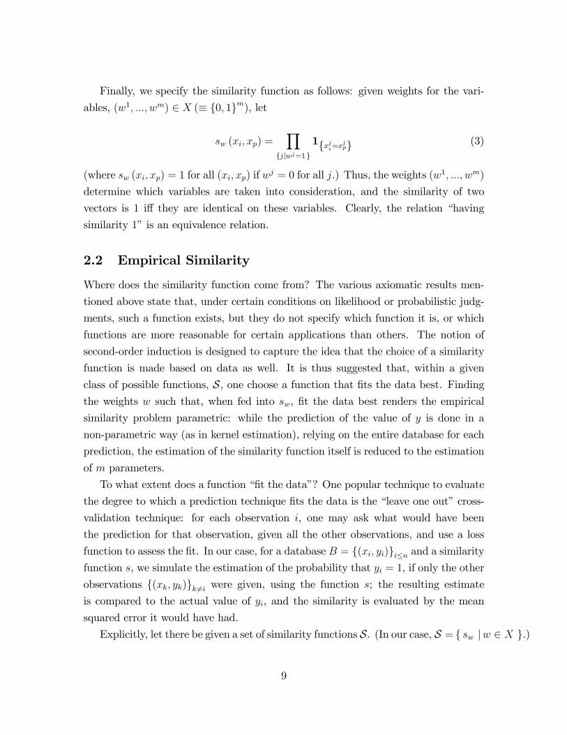
Finally, we specify the similarity function as follows: given weights for the vari-

ables, (w1, ..., wm) ∈ X (≡ {0, 1}m), let

sw (xi, xp) =∏

{j|wj=1}

1{xji=xjp} (3)

(where sw (xi, xp) = 1 for all (xi, xp) if wj = 0 for all j.) Thus, the weights (w1, ..., wm)

determine which variables are taken into consideration, and the similarity of two

vectors is 1 iff they are identical on these variables. Clearly, the relation “having

similarity 1”is an equivalence relation.

2.2 Empirical Similarity

Where does the similarity function come from? The various axiomatic results men-

tioned above state that, under certain conditions on likelihood or probabilistic judg-

ments, such a function exists, but they do not specify which function it is, or which

functions are more reasonable for certain applications than others. The notion of

second-order induction is designed to capture the idea that the choice of a similarity

function is made based on data as well. It is thus suggested that, within a given

class of possible functions, S, one choose a function that fits the data best. Findingthe weights w such that, when fed into sw, fit the data best renders the empirical

similarity problem parametric: while the prediction of the value of y is done in a

non-parametric way (as in kernel estimation), relying on the entire database for each

prediction, the estimation of the similarity function itself is reduced to the estimation

of m parameters.

To what extent does a function “fit the data”? One popular technique to evaluate

the degree to which a prediction technique fits the data is the “leave one out”cross-

validation technique: for each observation i, one may ask what would have been

the prediction for that observation, given all the other observations, and use a loss

function to assess the fit. In our case, for a database B = {(xi, yi)}i≤n and a similarityfunction s, we simulate the estimation of the probability that yi = 1, if only the other

observations {(xk, yk)}k 6=i were given, using the function s; the resulting estimate

is compared to the actual value of yi, and the similarity is evaluated by the mean

squared error it would have had.

Explicitly, let there be given a set of similarity functions S. (In our case, S = { sw |w ∈ X }.)

9

For s ∈ S, let

ysi =

∑k 6=i s(xk, xi)yk∑k 6=i s(xk, xi)

if∑

j 6=i s(xj, xi) > 0 and ysi = 0.5 otherwise. Define the mean squared error to be7

MSE (s) =

∑ni=1 (ysi − yi)

2

n.

It will be useful to define, for a set of variables indexed by J ⊆ M , the indicator

function of J , wJ , that is,

wlJ =

{1 l ∈ J0 l /∈ J

.

To simplify notation, we will use MSE (J) for MSE (swJ ).

The similarity functions we consider divide the database into sub-databases, or

“bins”, according to the values of the variables in J . Formally, for J ⊆ M and

z ∈ {0, 1}J , define the J-z bin to be the cases in B that correspond to these values8.

Formally, we will refer to the set of indices of these cases, that is,

b (J, z) ={i ≤ n

∣∣xji = zj ∀j ∈ J}

as “the J-z bin”.

It will also be convenient to define, for J ⊆ M , and z ∈ {0, 1}J , j ∈ M\J , andzj ∈ {0, 1}, the bin obtained from adding the value zj to z. We will denote it by

(J · j, z · zj

)= (J ∪ {j}, z′)

where z′l = zl for l ∈ J and z′j = zj.

Clearly, a set J ⊆ M defines 2|J | such bins (many of which may be empty).

A new point xp corresponds to one such bin. The probabilistic prediction for ypcorresponding to xp is the average frequency of 1’s in it. If a bin is empty, this

prediction is 0.5. Formally, the prediction is given by

y(J,z) =

∑i∈b(J,z) yi

|b (J, z)| (4)

7Similar results would hold for other loss functions. See subsection 4.1.8Splitting the database into such bins is clearly an artifact of the binary model. We analyze a

more realistic continuous model in Section 3.

10

if |b (J, z)| > 0 and y(J,z) = 0.5 otherwise.

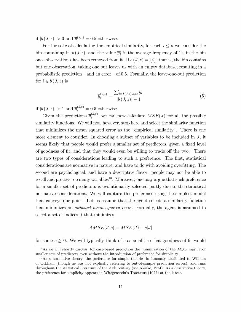
For the sake of calculating the empirical similarity, for each i ≤ n we consider the

bin containing it, b (J, z), and the value ysi is the average frequency of 1’s in the bin

once observation i has been removed from it. If b (J, z) = {i}, that is, the bin containsbut one observation, taking one out leaves us with an empty database, resulting in a

probabilistic prediction —and an error —of 0.5. Formally, the leave-one-out prediction

for i ∈ b (J, z) is

y(J,z)i =

∑k∈b(J,z),k 6=i yk

|b (J, z)| − 1(5)

if |b (J, z)| > 1 and y(J,z)i = 0.5 otherwise.

Given the predictions y(J,z)i , we can now calculate MSE(J) for all the possible

similarity functions. We will not, however, stop here and select the similarity function

that minimizes the mean squared error as the “empirical similarity”. There is one

more element to consider. In choosing a subset of variables to be included in J , it

seems likely that people would prefer a smaller set of predictors, given a fixed level

of goodness of fit, and that they would even be willing to trade off the two.9 There

are two types of considerations leading to such a preference. The first, statistical

considerations are normative in nature, and have to do with avoiding overfitting. The

second are psychological, and have a descriptive flavor: people may not be able to

recall and process too many variables10. Moreover, one may argue that such preference

for a smaller set of predictors is evolutionarily selected partly due to the statistical

normative considerations. We will capture this preference using the simplest model

that conveys our point. Let us assume that the agent selects a similarity function

that minimizes an adjusted mean squared error. Formally, the agent is assumed to

select a set of indices J that minimizes

AMSE(J, c) ≡MSE(J) + c|J |

for some c ≥ 0. We will typically think of c as small, so that goodness of fit would

9As we will shortly discuss, for case-based prediction the minimization of the MSE may favorsmaller sets of predictors even without the introduction of preference for simplicity.10As a normative theory, the preference for simple theories is famously attributed to William

of Ockham (though he was not explicitly referring to out-of-sample prediction errors), and runsthroughout the statistical literature of the 20th century (see Akaike, 1974). As a descriptive theory,the preference for simplicity appears in Wittgenstein’s Tractatus (1922) at the latest.

11

outweigh simplicity as theory selection criteria, but as positive, so that complexity

isn’t ignored. Given a cost c, we will refer to a similarity function s = swJ for

J ∈ arg minAMSE(J, c) as an empirical similarity function.

We now turn to analyze the properties of the empirical similarity, to address

the question of whether we should expect rational agents with access to a common

database to agree on their predictions.

2.3 Monotonicity

We start by showing that using a relatively small set of variables for prediction might

be desirable even with c = 0, because the goodness-of-fit (for a given database) can

decrease when adding one more predictor: MSE can be non-monotone with respect

to set inclusion.11 The reason is a version of the problem known as “the curse of

dimensionality”: more variables that are included in the determination of similarity

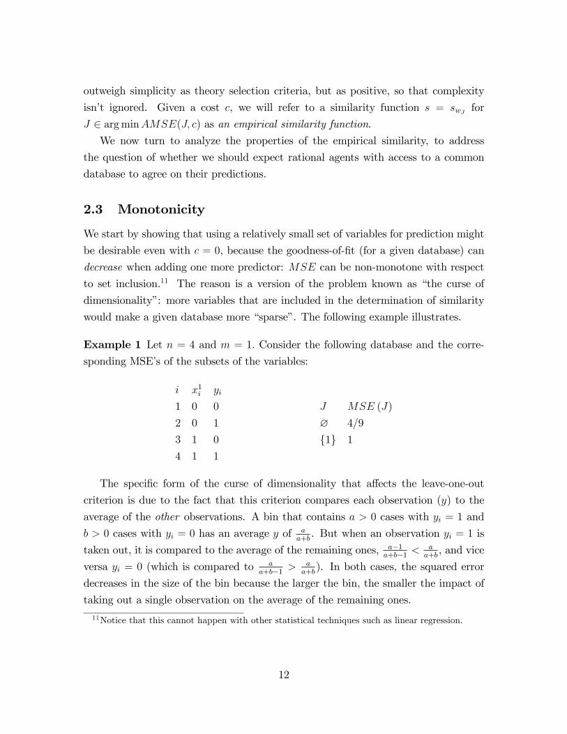
would make a given database more “sparse”. The following example illustrates.

Example 1 Let n = 4 and m = 1. Consider the following database and the corre-

sponding MSE’s of the subsets of the variables:

i x1i yi

1 0 0

2 0 1

3 1 0

4 1 1

J MSE (J)

∅ 4/9

{1} 1

The specific form of the curse of dimensionality that affects the leave-one-out

criterion is due to the fact that this criterion compares each observation (y) to the

average of the other observations. A bin that contains a > 0 cases with yi = 1 and

b > 0 cases with yi = 0 has an average y of aa+b. But when an observation yi = 1 is

taken out, it is compared to the average of the remaining ones, a−1a+b−1 <

aa+b, and vice

versa yi = 0 (which is compared to aa+b−1 >

aa+b). In both cases, the squared error

decreases in the size of the bin because the larger the bin, the smaller the impact of

taking out a single observation on the average of the remaining ones.

11Notice that this cannot happen with other statistical techniques such as linear regression.

12

The above suggests that in appropriately-defined “large”databases the curse of

dimensionality would be less severe and adding variables to the set of predictors would

be easier than in smaller databases. To make this comparison meaningful, and control

for other differences between the databases, we can compare a given database with

“replications”thereof, where the counters a and b above are replaced by ta and tb for

some t > 1. Formally, we will use the following definition.

Definition 1 Given two databases B = {(xi, yi)}i≤n and B′ = {(x′k, y′k)}k≤tn (fort ≥ 1), we say that B′ is a t-replica of B if, for every k ≤ tn, (x′k, y

′k) = (xi, yi) where

i = k(modn).

Consider a database B′ which is a t-replica of the database in Example 1. It can

readily be verified that

MSE (∅) =

(2t

4t− 1

)2<

(t

2t− 1

)2= MSE ({1}) .

Indeed, the dramatic difference of theMSE’s in Example 1 ([MSE ({1})−MSE (∅)])

is smaller for larger t’s, and converges to 0 as t → ∞. However, it is still positive.This suggests that there is something special about Example 1 beyond the size of

the database. Indeed, the variable in question, x1, is completely uninformative: the

distribution of y is precisely the same in each bin (i.e., for x1 = 0 and for x1 = 1), and

thus there is little wonder that splitting the database into these two bins can only

result in larger errors due to the smaller bin sizes, with no added explanatory power

to offset it. Formally, we define informativeness of a variable (for the prediction of y

in a database B) relative to a set of other variables as a binary property:

Definition 2 A variable j ∈ M is informative relative to a subset J ⊆ M\ {j} indatabase B = {(xi, yi)}i≤n if there exists z ∈ {0, 1}J such that |b (J, z · 0)| , |b (J, z · 1)| >0 and

y(J ·j,z·0) 6= y(J ·j,z·1).

In other words, a variable xj is informative for a subset of the variables, J , if, for

at least one assignment of values to these variables, the relative frequency of y = 1 in

the bin defined by these values and xj = 1 and the relative frequency defined by the

same values and xj = 0 are different.

13

One reason that a variable j may be uninformative relative to a set of other

variables is that it can be completely determined by them. Formally,

Definition 3 A variable j ∈ M is a function of J ⊆ M\ {j} in database B =

{(xi, yi)}i≤n if there is a function f : {0, 1}J → {0, 1} such that, for all i ≤ n,

xji = f((xki)k∈J

).

If j is a function of J , the bins defined by J and by J∪{j} are identical, and clearlyj cannot be informative relative to J . However, as we saw above, a variable j may fail

to be informative relative to J also if it isn’t a function of J . To determine whether

j is a function of J we need not consult the y values. Informativeness, by contrast, is

conceptually akin to correlation of the variable xj with y given the variables in J .

We can finally state conditions under which more variables are guaranteed to

result in a lower MSE. Intuitively, we want to start by adding a variable that is

informative (relative to those already in use), and to make sure that the database

isn’t split into too small bins. Formally,

Proposition 1 Assume that j is informative relative to J ⊆M\ {j} in the databaseB = {(xi, yi)}i≤n. Then there exists a T ≥ 1 such that, for all t ≥ T , for a t-replica of

B,MSE (J ∪ {j}) < MSE (J). Conversely, if j is not informative relative to J , then

for any t-replica of B, MSE (J ∪ {j}) ≥ MSE (J), with a strict inequality unless j

is a function of J .

We note in passing that informativeness of a variable does not satisfy monotonicity

with respect to set inclusion:

Observation 1 Let there be given a database B = {(xi, yi)}i≤n, a variable j ∈ M ,and two subsets J ⊆ J ′ ⊆ M\ {j}. It is possible that j is informative for J , but notfor J ′ as well as vice versa.

2.4 Uniqueness

We have seen in section 2.3 that monotonicity of theMSE is not generally guaranteed.

Immediate implications are that the best fit is not necessarily achieved by a unique

subset of variables J , and in particular by the full set of all available predictors

(J = M). For concreteness, consider the following database

14

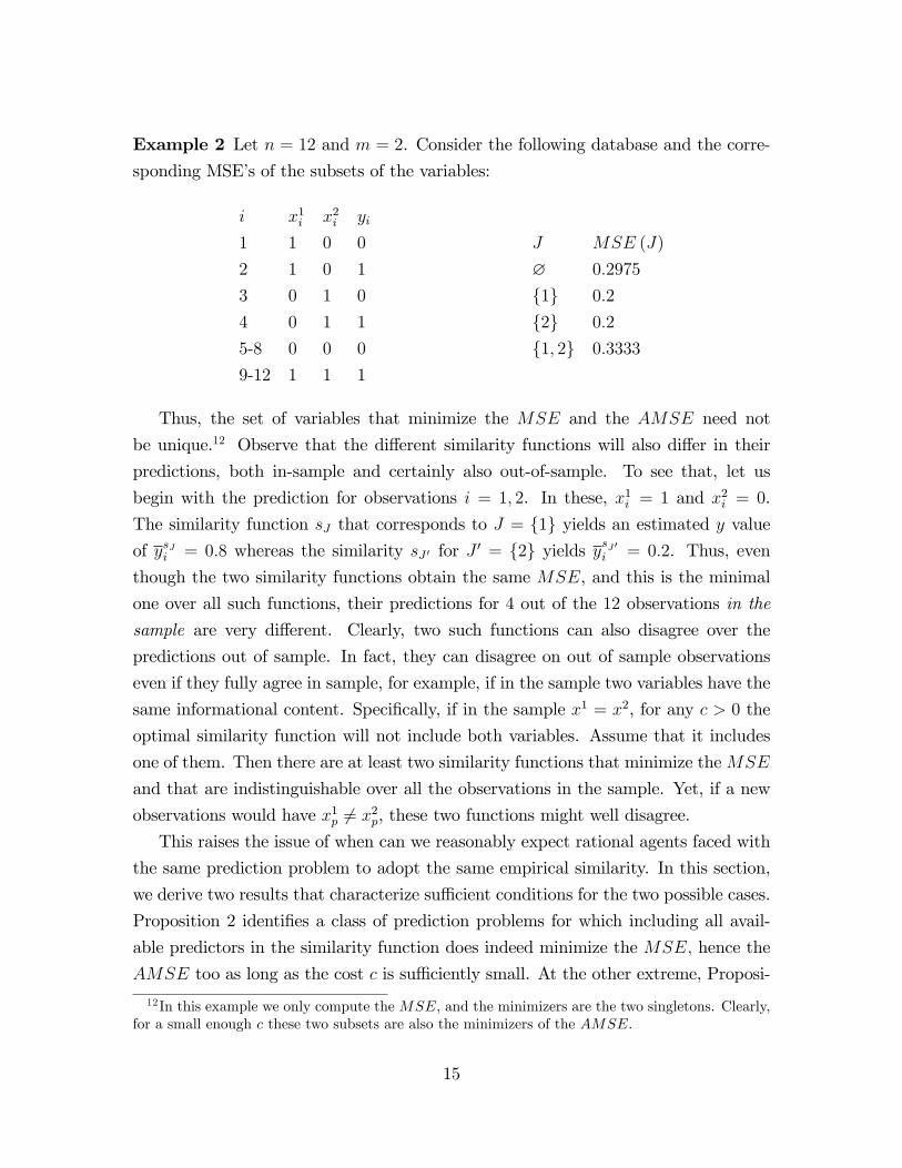
Example 2 Let n = 12 and m = 2. Consider the following database and the corre-

sponding MSE’s of the subsets of the variables:

i x1i x2i yi

1 1 0 0

2 1 0 1

3 0 1 0

4 0 1 1

5-8 0 0 0

9-12 1 1 1

J MSE (J)

∅ 0.2975

{1} 0.2

{2} 0.2

{1, 2} 0.3333

Thus, the set of variables that minimize the MSE and the AMSE need not

be unique.12 Observe that the different similarity functions will also differ in their

predictions, both in-sample and certainly also out-of-sample. To see that, let us

begin with the prediction for observations i = 1, 2. In these, x1i = 1 and x2i = 0.

The similarity function sJ that corresponds to J = {1} yields an estimated y valueof ysJi = 0.8 whereas the similarity sJ ′ for J ′ = {2} yields ysJ′i = 0.2. Thus, even

though the two similarity functions obtain the same MSE, and this is the minimal

one over all such functions, their predictions for 4 out of the 12 observations in the

sample are very different. Clearly, two such functions can also disagree over the

predictions out of sample. In fact, they can disagree on out of sample observations

even if they fully agree in sample, for example, if in the sample two variables have the

same informational content. Specifically, if in the sample x1 = x2, for any c > 0 the

optimal similarity function will not include both variables. Assume that it includes

one of them. Then there are at least two similarity functions that minimize theMSE

and that are indistinguishable over all the observations in the sample. Yet, if a new

observations would have x1p 6= x2p, these two functions might well disagree.

This raises the issue of when can we reasonably expect rational agents faced with

the same prediction problem to adopt the same empirical similarity. In this section,

we derive two results that characterize suffi cient conditions for the two possible cases.

Proposition 2 identifies a class of prediction problems for which including all avail-

able predictors in the similarity function does indeed minimize the MSE, hence the

AMSE too as long as the cost c is suffi ciently small. At the other extreme, Proposi-

12In this example we only compute the MSE, and the minimizers are the two singletons. Clearly,for a small enough c these two subsets are also the minimizers of the AMSE.

15

tion 3 identifies a class of prediction problems for which at least two disjoint subsets

of variables minimize MSE and AMSE. The comparison between the conditions

in Propositions 2 and 3 sheds light on features of a prediction problem that make

agreement among rational agents more or less likely to occur.

Let us first consider data generating processes that are conducive to the inclusion

of all variables in the empirical similarity. Assume that the values of the predictors,

(xi) are i.i.d. with a joint distribution g on X, and that yi = f (xi) for a fixed

f : X → {0, 1}.13 Let us refer to this data generating process as (g, f). We introduce

the following definition, then present our result:

Definition 4 A variable j ∈ M is informative for (g, f) if there are values z−j =(zk)k 6=j such that (i) f (z−j · 0) 6= f (z−j · 1); and (ii) g (z−j · 0) , g (z−j · 1) > 0, where

z · q ∈ X is the vector obtained by augmenting z−jwith zj = q for q ∈ {0, 1}.

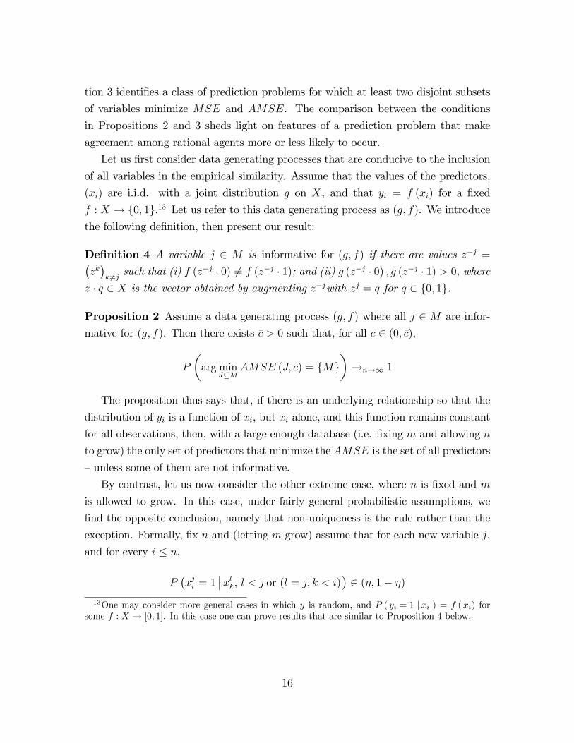
Proposition 2 Assume a data generating process (g, f) where all j ∈ M are infor-

mative for (g, f). Then there exists c > 0 such that, for all c ∈ (0, c),

P

(arg min

J⊆MAMSE (J, c) = {M}

)→n→∞ 1

The proposition thus says that, if there is an underlying relationship so that the

distribution of yi is a function of xi, but xi alone, and this function remains constant

for all observations, then, with a large enough database (i.e. fixing m and allowing n

to grow) the only set of predictors that minimize the AMSE is the set of all predictors

—unless some of them are not informative.

By contrast, let us now consider the other extreme case, where n is fixed and m

is allowed to grow. In this case, under fairly general probabilistic assumptions, we

find the opposite conclusion, namely that non-uniqueness is the rule rather than the

exception. Formally, fix n and (letting m grow) assume that for each new variable j,

and for every i ≤ n,

P(xji = 1

∣∣xlk, l < j or (l = j, k < i))∈ (η, 1− η)

13One may consider more general cases in which y is random, and P ( yi = 1 |xi ) = f (xi) forsome f : X → [0, 1]. In this case one can prove results that are similar to Proposition 4 below.

16

for a fixed η ∈ (0, 0.5). That is, we consider a rather general joint distribution of

the variables xj =(xji)i≤n, with the only constraint that the probability of the next

observed value, xji , being 1 or 0, conditional on all past observed values, is uniformly

bounded away from 0, where “past”is read to mean “an observation of a lower-index

variable or an earlier observation of the same variable”. For such a process we can

state:

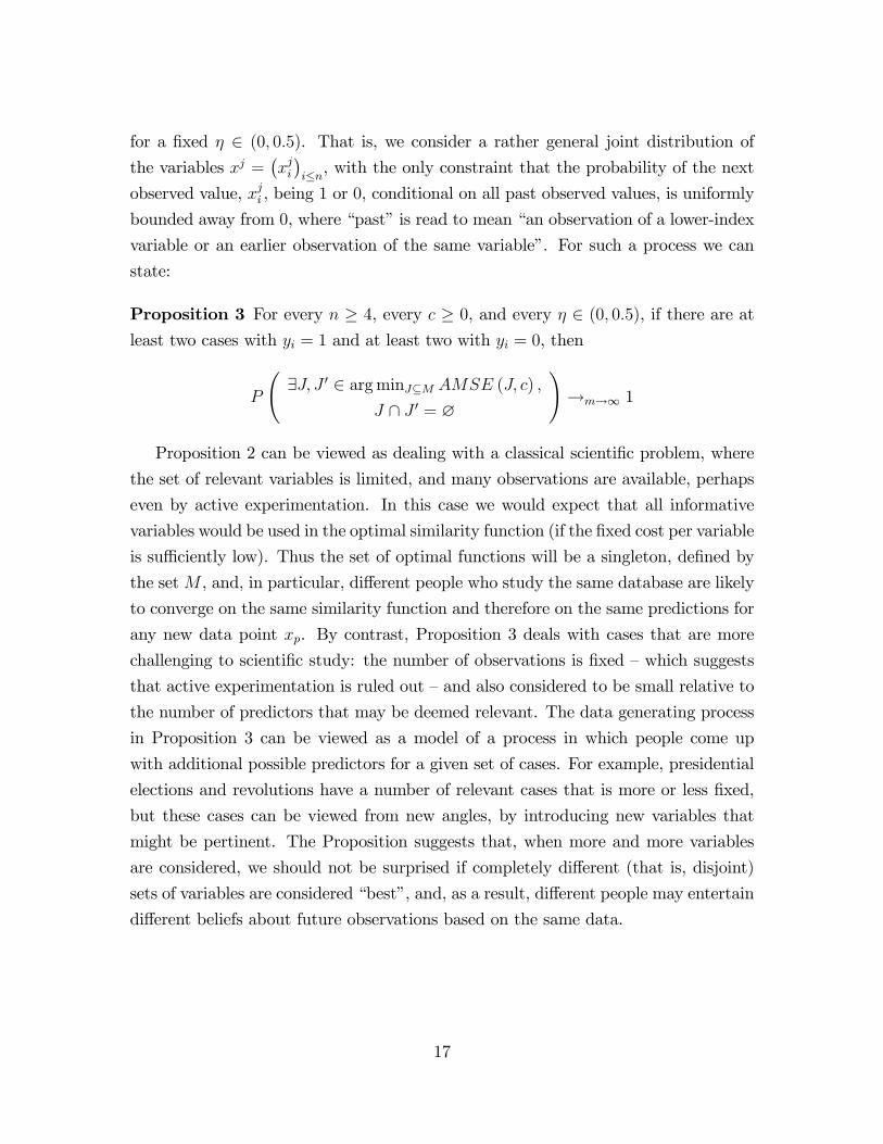
Proposition 3 For every n ≥ 4, every c ≥ 0, and every η ∈ (0, 0.5), if there are at

least two cases with yi = 1 and at least two with yi = 0, then

P

(∃J, J ′ ∈ arg minJ⊆M AMSE (J, c) ,

J ∩ J ′ = ∅

)→m→∞ 1

Proposition 2 can be viewed as dealing with a classical scientific problem, where

the set of relevant variables is limited, and many observations are available, perhaps

even by active experimentation. In this case we would expect that all informative

variables would be used in the optimal similarity function (if the fixed cost per variable

is suffi ciently low). Thus the set of optimal functions will be a singleton, defined by

the setM , and, in particular, different people who study the same database are likely

to converge on the same similarity function and therefore on the same predictions for

any new data point xp. By contrast, Proposition 3 deals with cases that are more

challenging to scientific study: the number of observations is fixed —which suggests

that active experimentation is ruled out —and also considered to be small relative to

the number of predictors that may be deemed relevant. The data generating process

in Proposition 3 can be viewed as a model of a process in which people come up

with additional possible predictors for a given set of cases. For example, presidential

elections and revolutions have a number of relevant cases that is more or less fixed,

but these cases can be viewed from new angles, by introducing new variables that

might be pertinent. The Proposition suggests that, when more and more variables

are considered, we should not be surprised if completely different (that is, disjoint)

sets of variables are considered “best”, and, as a result, different people may entertain

different beliefs about future observations based on the same data.

17

2.5 Complexity

Examples in which different sets of variables obtain precisely the same, minimal

AMSE might be knife-edge, hence disagreement might appear to be unlikely to occur

in practice. In this section, we present a second reason why rational agents faced with

the same prediction problem might adopt different similarity functions and disagree

in their predictions. As the number of possible predictors in a database grows, so does

the complexity of finding the optimal set of variables, even if it is unique. Formally,

we define the following problem:

Problem 1 EMPIRICAL-SIMILARITY: Given integers m,n ≥ 1, a database B =

{(xi, yi)}i≤n, and (rational) numbers c, R ≥ 0, is there a set J ⊆M ≡ {1, ...,m} suchthat AMSE(J, c) ≤ R?

Thus, EMPIRICAL-SIMILARITY is the yes/no version of the optimization prob-

lem, “Find the empirical similarity for database B and constant c”. We can now

state

Theorem 1 EMPIRICAL-SIMILARITY is NPC.

It follows that, when many possible variables exist, we should not assume that

people can find an (or the) empirical similarity. That is, it isn’t only the case that

there are 2m different subsets of variables, and therefore as many possible similarity

functions to consider. There is no known algorithm that can find the optimal simi-

larity in polynomial time, and it seems safe to conjecture that none would be found

in the near future.14 Clearly, the practical import of this complexity result depends

crucially on the number of variables, m.15 For example, if m = 2 and there are only 4

subsets of variables to consider, it makes sense to assume that people find the “best”

one. Moreover, if n is large, the best one may well be all the informative variables.16

14This result is the equivalent of the main result in Aragones et al. (2005) for regression analysis.Thus, both in rule-based models and in case-based models of reasoning, it is a hard problem to finda small set of predictors that explain the data well.15Indirectly, it also depends on n. If n is bounded, there can be only a bounded number (2n) of

different variable values, and additional ones need not be considered.16If we restrict EMPIRICAL-SIMILARITY to accept problems with a bounded m, say, m ≤ m0,

then it obviously becomes polynomial (in n, involving coeffi cients of the order of magnitude of 2m).

18

3 A Continuous Model

One can extend the model to deal with continuous variables, allowing the predictors

(x1, ..., xm) to assume values (jointly) in a set X ⊆ Rm while the predicted variable,y, — in a set Y ⊆ R. It is natural to use the same formulae of similarity-weightedaverage used for the binary case, i.e.,

ysp =

∑i≤n s(xi, xp)yi∑i≤n s(xi, xp)

(6)

this time interpreted as the predicted value of y (rather than the estimation of the

probability that it be 1). This formula was axiomatized in Gilboa, Lieberman, and

Schmeidler (2006).17 In case s(xi, xp) = 0 for all i ≤ n, we set ysp = y0 for an arbitrary

value y0 ∈ Y .18

For many purposes it makes sense to consider more general similarity functions,

that would allow for values in the entire interval [0, 1] and would not divide the

database into neatly separated bins. In particular, Billot, Gilboa, and Schmeidler

(2008) characterize similarity functions of the form

s (x, x′) = e−n(x,x′)

where n is a norm on Rm. Indeed, this functional form is often used in explaining

psychological data about classification problems.19 Gilboa, Lieberman, and Schmei-

dler (2006) and Gayer, Gilboa, Lieberman (2007) also study the case of a weighted

17If Y is discrete, we may also define the predicted value of yp by

ysp ∈ arg maxy

∑i≤n

s(xi, xp)1{y=yi} (7)

which is equivalent to kernel classification and has been axiomatized in Gilboa and Schmeidler(2003).18We choose some value y0 only to make the expression ysp well-defined. Its choice will have no

effect on our analysis.19Shepard (1987) suggests that a similarity function which is exponential in distance (in a “psy-

chological space”) might be a ‘universal law of generalization.’See Nosofsky (2014) for a more recentsurvey. Note, however, that the similarity function in that literature is mostly for a classificationtask, rather than for probability estimation.

19

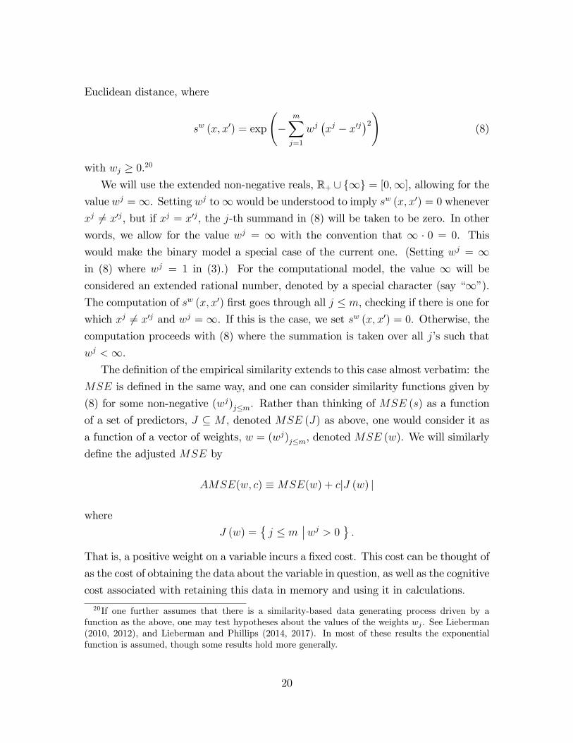
Euclidean distance, where

sw (x, x′) = exp

(−

m∑j=1

wj(xj − x′j

)2)(8)

with wj ≥ 0.20

We will use the extended non-negative reals, R+ ∪ {∞} = [0,∞], allowing for the

value wj =∞. Setting wj to∞ would be understood to imply sw (x, x′) = 0 whenever

xj 6= x′j, but if xj = x′j, the j-th summand in (8) will be taken to be zero. In other

words, we allow for the value wj = ∞ with the convention that ∞ · 0 = 0. This

would make the binary model a special case of the current one. (Setting wj = ∞in (8) where wj = 1 in (3).) For the computational model, the value ∞ will be

considered an extended rational number, denoted by a special character (say “∞”).The computation of sw (x, x′) first goes through all j ≤ m, checking if there is one for

which xj 6= x′j and wj =∞. If this is the case, we set sw (x, x′) = 0. Otherwise, the

computation proceeds with (8) where the summation is taken over all j’s such that

wj <∞.The definition of the empirical similarity extends to this case almost verbatim: the

MSE is defined in the same way, and one can consider similarity functions given by

(8) for some non-negative (wj)j≤m. Rather than thinking of MSE (s) as a function

of a set of predictors, J ⊆ M , denoted MSE (J) as above, one would consider it as

a function of a vector of weights, w = (wj)j≤m, denoted MSE (w). We will similarly

define the adjusted MSE by

AMSE(w, c) ≡MSE(w) + c|J (w) |

where

J (w) ={j ≤ m

∣∣wj > 0}.

That is, a positive weight on a variable incurs a fixed cost. This cost can be thought of

as the cost of obtaining the data about the variable in question, as well as the cognitive

cost associated with retaining this data in memory and using it in calculations.

20If one further assumes that there is a similarity-based data generating process driven by afunction as the above, one may test hypotheses about the values of the weights wj . See Lieberman(2010, 2012), and Lieberman and Phillips (2014, 2017). In most of these results the exponentialfunction is assumed, though some results hold more generally.

20

However, when we think of an empirical similarity as a function sw that minimizes

the AMSE, we should bear in mind the following.

Observation 2 There are databases for which

arg minw∈[0,∞]m

MSE (w) = ∅.

(This Observation is proved in the Appendix.) The reason that the argmin of the

MSE may be empty is that the MSE is well-defined at wj = ∞ but need not be

continuous there. We will therefore be interested in vectors w that obtain the lowest

MSE approximately.

We can define approximately optimal similarity: for ε > 0 let

ε- arg minAMSE ={w ∈ [0,∞]m

∣∣∣AMSE (w, c) ≤ infw′AMSE (w′, c) + ε

}Thus, the ε-arg minAMSE is the set of weight vectors that are ε-optimal. We are

interested in the shape of this set for small ε > 0.

3.1 Almost-Uniqueness

We argue that the main messages of our results in the binary case carry over to

this model as well. Again, the key questions are the relative sizes of n and m, and

the potential causal relationships between observations: when there are n >> m

independent observations that obey a functional rule y = f (x) —which, in particular,

implies that xi contains enough information to predict yi —the optimal weights will be

unique, and different people are likely to converge to the same opinion. By contrast,

whenm >> n, it is likely that different sets of variable will explain the same (relatively

small) set of observations.

Let us first consider the counterpart of (g, f) processes, where the observations

(xi, yi) are i.i.d. For simplicity, assume that each xji and each yi is in the bounded

interval [−K,K] for K > 0. Let g be the joint density of x, with g (z) ≥ η > 0

for all x ∈ X ≡ [−K,K]mand let a continuous f : X → [−K,K] be the underlying

21

functional relationship between x and y so that21

yi = f (xi) .

Refer to this data generating process as (g, f).

Proposition 4 Assume a data generating process (g, f) (where f is continuous). Let

there be given ν, ξ > 0. There are an integer N0 and W0 ≥ 0 such that for every

n ≥ N0, the vector w0 defined by wj0 = W0 satisfies

P (MSE (w0) < ν) ≥ 1− ξ.

The proposition says that, if there is an underlying relationship so that yi is a

continuous function of xi, and this function remains constant for all observations,

then, when the database is large enough, with very high probability, this relationship

can be uncovered. This is a variation on known results about convergence of kernel

estimation techniques (see Nadaraya, 1964, Watson, 1964) and it is stated and proved

here only for the sake of completeness.22

We take Proposition 4 as suggesting that, under the assumption of the (g, f)

process, different individuals are likely to converge to similar beliefs about the value

of yp for a new case given by xp within the known range. The exact similarity function

that different people may choose may not always be identical. For example, if x1i = x2i

for every observation in the database, one function sw may obtain a near-perfect fit

with w1 >> 0 and w2 = 0 and another, sw′, — with w′1 = 0 and w′2 >> 0. If

one individual uses sw to make predictions, and another — sw′, they will agree on

the predicted values for all x that are similar to those they have encountered in the

database. In a sense, they may agree on the conclusion but not on the reasoning. But,

as long as they observe cases in which x1 = x2, they will not have major disagreements

about any particular prediction.

However, we also have a counterpart of Proposition 3: given n,m, assume that

for each i ≤ n, yi is drawn, given (yk)k<i, from a continuous distribution on [−K,K]

with a continuous density function hi bounded below by η > 0. Let v be a lower

21Similar conclusion would follow if we allow yi to be distributed around f (xi) with an i.i.d. errorterm.22We are unaware of a statement of a result that directly implies this one, though there are many

results about optimal bandwidth that are similar in spirit.

22

bound on the conditional variance of yi (given its predecessors). Next assume that,

for every j ≤ m and i ≤ n, given (yi)i≤n,(xli)i≤n,l<j, and

(xji)k<i, xji is drawn from

a continuous distribution on [−K,K] with a continuous conditional density function

gji bounded below by η > 0. Thus, as in Proposition 3, we allow for a rather general

class of data generating processes, where, in particular, the x’s are not constrained to

be independent.23 The message of the following result is that the empirical similarity

is non-unique.

For such a process we can state:

Proposition 5 Let there be given c ∈ (0, v/2). There exists ε > 0 such that for all

ε ∈ (0, ε) and for every δ > 0 there exists N such that for every n ≥ N there exists

M (n) such that for every m ≥M (n),

P (ε- arg minAMSE is not connected) ≥ 1− δ.

The fact that the ε-arg minAMSE is not a singleton is hardly surprising, as we

allow the AMSE to be ε-away from its minimal value. However, one could expect

this set to be convex, as would be the case if we were considering the minimization

of a convex function. This convexity would also suggest a simple follow-the-gradient

algorithm to find a global minimum of the AMSE function. But the Proposition

states that this is not the case. For ε = 0 we could expect ε-arg minAMSE to be

a singleton (hence a convex set), but as soon as ε > 0 we will find that there are

ε-minimizers of the AMSE whose convex combinations need not be ε-minimizers.

Clearly, this is possible because our result is asymptotic: given ε we let n, and

then m ≥ M (n) go to infinity. But we find the present order of quantifiers to be

natural: ε indicates a degree of tolerance to suboptimality, and it can be viewed as a

psychological feature of the agent, as can the cost c. The pair (ε, c) can be considered

as determining the agent’s preferences for the accuracy and simplicity trade-off. An

agent with given preferences is confronted with a database, and we ask whether her

“best”explanation of the database be unique as more data accumulate. Proposition

5 suggests that multiplicity of local optima of the similarity function is the rule when

the number of variables is allowed to increase relative to that of the observations.23The assumption of independence of the yi’s is only used to guarantee that each observation yi

has suffi ciently close other observations, and it can therefore be significantly relaxed.

23

3.2 Complexity

Importantly, our complexity result extends to the continuous case. Formally,

Problem 2 CONTINUOUS-EMPIRICAL-SIMILARITY: Given integers m,n ≥ 1,

a database of rational valued observations, B = {(xi, yi)}i≤n, and (rational) numbersc, R ≥ 0, is there a vector of extended rational non-negative numbers w such that

AMSE(w, c) ≤ R?

And we can state

Theorem 2 CONTINUOUS-EMPIRICAL-SIMILARITY is NPC.

As will be clear from the proof of this result, the key assumption that drives the

combinatorial complexity is not that x, y or even w are binary. Rather, it is that

there is a fixed cost associated with including an additional variable in the similarity

function. That is, that the AMSE is discontinuous at wj = 0.2425

To conclude, it appears that the qualitative conclusion, namely that people may

have the same database of cases yet come up with different “empirical similarity”

functions to explain it, would hold also in a continuous model.

4 Discussion

4.1 Robustness of the Results

There are a number of modeling decisions to be made in order to state formal results

as those above, including the ranges of the variables, of the similarity functions, of the

weights therein, as well as the loss functions used to measure the in-sample fit, and

the cross validation criterion. Our choices were guided by what seemed the simplest

and/or most commonly used definitions, and yet one may wonder how robust are the

results.24To see that this complexity result does not hinge on specific values of the variables xji and each

yi, one may prove an analogous result for a problem in which positive-length ranges of values aregiven for these variables, where the question is whether a certain AMSE can be obtained for somevalues in these ranges.25See also Eilat (2007), who finds that the fixed cost for including a variable is the main driving

force behind the complexity of finding an optimal set of predictors in a regression problem (as inAragones et al., 2005).

24

Let us first comment on the ranges of the variables: we study here two extreme

cases, one in which all variables are in {0, 1}, and the other in which they are con-tinuous. The former seems best suited to clarify conceptual issues, but it may be

oversimplified in some ways. (In particular, in our model similarity is a binary rela-

tion which is also transitive.) The latter model is obviously more flexible, but requires

messier statements of the results. As the same conceptual results hold in both, one

may speculate that this will be the case for various intermediate cases (say, continuous

variables with a binary similarity function, or vice versa).

The selection criteria for the optimal similarity function are not crucial for most

of our results. In fact, the results are all based on perfect fits: Propositions 2 and

4 state that, with high probability, a perfect fit will be obtained only by including

all informative variables, thus resulting in a unique set of variables (in the binary

model), or an almost-unique collection of weights (in the continuous one). By contrast,

Propositions 3 and 5, which state that, with very high probability the (ε-)optimal

similarity function will not be unique also rely on perfect fits, only this time a perfect

fit that is obtained by disjoint sets of variables. Finally, the complexity results are

also based on a perfect fit which is equivalent to a perfect set cover. When perfect fit

is involved, most selection criteria agree. In particular, we need a loss function and

a cross-validation technique that yields 0 loss if, and only if, a perfect fit is obtained

in-sample.

The only important assumption for the complexity results (Theorems 1 and 2)

is the discontinuity of the AMSE near zero weights. That is, we assume, in a way

that’s similar to the adjusted R2 in linear regression, that there is a minimal fixed

cost to be paid for the inclusion of a variable (that is, to have a positive weight for

that variable). This discontinuity at 0 adds the combinatorial aspect to the AMSE

minimization problem, and allows the reduction of combinatorial problems as in our

proofs. Our complexity results do not directly generalize to an objective function

that is continuous at zero. Furthermore, it is possible that they do not hold in

this case.26 However, as explained above, we find the discontinuous cost function

rather reasonable: the difference between a weight wj > 0 and wj = 0 involves the

need to collect and recall data about the variable, to use another variable in making

computations, and so forth. It seems that some cost is incurred by the inclusion of a

26Eilat (2007) proves, in the context of linear regression, that Aragones et al. (2005) complexityresult holds if the cost function is discontinuous at zero, but not otherwise.

25

variable, and that this cost isn’t entirely negligible if we think of the model as trying

to capture a cognitive process people undergo in trying to make predictions.

4.2 Learnability

Our analysis can be viewed as adding to a large literature on what can and what

cannot be learnt. We consider the problem of predicting yp based on a database

(xi, yi)i≤n and the value of xp. One can distinguish among three types of set-ups:

(i) There exists a basic functional relationship, y = f (x), where one may obtain

observations of y for any x one chooses to experiment with;

(ii) There exists a basic functional relationship, y = f (x), and one may obtain

i.i.d. observations (x, y), but can’t control the observed x’s;

(iii) There is no bounded set of variables x such that yi depends only on xi,

independently of past values.

Set-up (i) is the gold standard of scientific studies. It allows testing hypotheses,

distinguishing among competing theories and so forth. However, many problems in

fields such as education or medicine are closer to set-up (ii). In these problems one

cannot always run controlled experiments, be it due to the cost of the experiments,

their duration, or the ethical problems involved. Still, statistical learning is often

possible. The theory of statistical learning (see Vapnik, 1998) suggests the VC di-

mension of the set of possible functional relationships as a litmus test for the classes

of functions that can be learnt and those that cannot. Finally, there are problems

that are closer to set-up (iii). The rise and fall of economic empires, the ebb and

flow of religious sentiments, social norms and ideologies are all phenomena that affect

economic predictions, yet do not belong to problems of types (i) or (ii). In particular,

there are many situations in which there is causal interaction among different obser-

vations, as in autoregression models. In this case we cannot assume an underlying

relationship y = f (x), unless we allow the set of variables x to include past values of

y, thereby letting m grow with n.

Our results are in line with the general message of statistical learning theory.

Specifically, our positive learning results, namely, Propositions 2 and 4, assume that

there is an underlying functional relationship of the type y = f (x), keep m fixed and

let n grow to infinity. The fact that learning is possible under these circumstances

may not seem like a major surprise. Observe, however, that our results do not deal

26

with learning the function f directly and, for that reason, they do not directly follow

from results about classes of functions with a low VC dimension. In particular, in our

model the prediction of y is always done non-parametrically, by weighted averages

of other y values, rather than by some direct function of the x variables. In this

context, our learning results should be interpreted as saying that if, unbeknownst to

the agent, y is a function of x, but the agent adheres to case-based prediction as she

usually does, she is likely to make correct predictions even though she is ignorant of

the nature of the underlying process.

Our negative results (Propositions 3 and 5) may also sound familiar: with few

observations and many variables, learning is not to be expected. However our notion

of a negative result is starker than that used in the bulk of the literature: we are not

dealing with failures of convergence with positive probability, but with convergence to

multiple limits. In particular, we conclude that, with very high probability, there will

be vastly different similarity functions, each of which obtains a perfect fit to the data.

When applied to the generation of beliefs by economic agents, our results discuss the

inevitability of large differences in opinion. Finally, our complexity results (Theorems

1 and 2), which also point at inability of learning, seem to have no obvious counterpart

in the literature. Importantly, these results show that learning might be diffi cult even

in the simple process discussed here (and justified by psychological research).

4.3 Compatibility with Bayesianism

There are several ways in which the learning process we study can relate to the

Bayesian approach. First, one may consider our model as describing the generation

of prior beliefs, along the lines of the “small world”interpretation of the state space

(as in Savage, 1954, section 5.5). In the examples discussed above this “prior”would

be summarized by a single probability number, and there wouldn’t be any opportunity

to perform Bayesian updating. One may develop slightly more elaborate models, in

which each case would involve a few stages (say, demonstrations, reaction by the

regime, siege of parliament...) and use past cases to define a prior on the multi-stage

space, which can be updated after some stages have been observed. Our approach

is compatible with this version of Bayesianism, where the similarity-based relative

frequencies using the empirical similarity is a method of generating a prior belief over

the state space.

27

Alternatively, one can adopt a “large world” or “grand state space” approach,

in which a state of the world resolves any uncertainty from the beginning of time.

Savage (1954) suggests to think of a single decision problem in one’s life, as if one

were choosing a single act (strategy) upon one’s birth. Thus, the newborn baby

would need to have a prior over all she may encounter in her lifetime. For many

applications one may need to consider historical cases, and thus the prior should be

the hypothetical one the decision maker would have had, had she been born years

back. The assumption that newborn entertain a prior probability over the entire

paths their lives would take is a bit fanciful. Further, the assumption that they

would have such a prior even before they could make any decisions conflicts with

the presumably-behavioral foundations of subjective probability. Yet, this approach

is compatible with the process we describe: in the language of such a model, ours

can be described as agents having a high prior probability that the data generating

process would follow the empirical similarity function. In the context of a game (such

as a revolution), this would imply that they expect other players’beliefs to follow a

similar process.

There are ways of implementing the Bayesian approach that are in between the

small world and the large world interpretation, and these are unlikely to be compatible

with our model. For example, assume that an agent believes that the successes of

revolutions generates a (conditionally) i.i.d. sequence of Bernoulli random variables,

with an unknown parameter p. As a Bayesian statistician, she has a prior probability

over p, and she observes past realizations in order to infer what p is likely to be. This

Bayesian updating of the prior over p to a posterior has no reason to resemble our

process of learning the similarity function.

In this paper we focus on probabilistic beliefs, or point estimates of the variable y

given the x’s. In case of uniqueness of the similarity function, or at least agreement

among all the empirical similarity functions, one may consider these estimates to be

objective, and proceed to assume that all rational agents would share them. But in

case of disagreement, one may ask whether it is rational for the agents to disagree.

For example, if there are multiple similarity functions that obtain a best fit, is it

rational for an agent to choose one and based her predictions on that function alone?

Wouldn’t it more rational for her, assuming unbounded computational ability, to find

all optimal functions and somehow take them into account in her predictions? These

are valid questions which are beyond the scope of this paper.

28

4.4 Agreement

Economic theory tends to assume that, given the same information, rational agents

would entertain the same beliefs: differences in beliefs can only arise from asymmetric

information. In the standard Bayesian model, this assumption is incarnated in the

attribution of the same prior probability to all agents, and it is referred to as the

“Common Prior Assumption”. Differences in beliefs cannot be commonly known, as

proved by Aumann (1976) in the celebrated “agreeing to disagree”result.

The Common Prior Assumption has been the subject of heated debates (see Mor-

ris, 1995, Gul, 1998, as well as Brandenburger and Dekel, 1987 in the context of Au-

mann, 1987). We believe that studying belief formation processes might shed some

light on the reasonability of this assumption. Specifically, when adopting a small

worlds view, positive learning results (such as Propositions 2 and 4) can identify

economic set-ups where beliefs are likely to be in agreement. By contrast, negative

results (such as Propositions 3 and 5) point to problems where agreement is less likely

to be the case.

In Argenziano and Gilboa (2018) we apply this approach to equilibrium selection

in coordination games. We study in detail the extreme case of adding a single variable

to the similarity function in the binary model: assuming that there is agreement about

the other set of relevant variables, J , will a new variable j /∈ J be added to it? This isabout as small as a small world can be, and we interpret our analysis in that paper as

shared by all players in the game. By contrast, when the number of variables grows,

players may play off-equilibrium due to the negative results proved above.

4.5 Higher-Order Induction Processes

Second-order processes raise questions about yet higher order processes of the same

nature, and the possibility of infinite regress. The question then arises, why do we

focus on second-order induction and do not climb up the hierarchy of higher-order

inductive processes? Higher order induction can indeed be defined in the context of

our model. Our notion of second-order induction consists of learning the similarity

function from the database of observation. One may well ask, could this learning

process be improved upon? For example, we have been using a leave-one-out tech-

nique. But the literature suggests also other methods, such as k-fold cross-validation,

in which approximately 1/k of the database is taken out each time, and their y values

29

are estimated by the remaining observations. One can consider, for a given data-

base, the choice of an optimal k, or compare these methods to bootstrap methods

(see, for instance, Kohavi, 1995). Similarly, kernel methods can be compared to

nearest-neighbor methods (Fix and Hodges, 1951, 1952). In short, the process we

assume in this paper, of second-order induction, can itself be learnt by what might be

called third-order induction, and an infinite regress can be imagined. Isn’t restricting

attention to second-order induction somewhat arbitrary? Is it a result of bounded

rationality?

A few comments are in order. First, in some types of applications lower orders may

provide good approximations. For example, suppose that it is indeed the case that

y = f (x) as in Propositions 2 and 4. Zero-order induction may refer to the assumption

that there is nothing to be learnt from the past about the future, or, at least, that

the x variables contain no relevant information. This would surely lead to poor

predictions as compared to the learnable process (y = f (x)). First-order induction

would be using a fixed similarity function to predict y based on its past values. This

would provide much better estimates, though also systematic biases (in particular,

near the boundaries of the domain of x). Thus, second-order induction is needed,

which, in particular, leads to higher weights, and “tighter” similarity functions for

large n. This is basically the message of Propositions 2 and 4: similarly to decreasing

the bandwidth of the Nadaraya-Watson estimator when n increases, computing the

empirical similarity leads (with very high probability) to convergence of the estimator

to yp = f (xp). Third-order induction could improve these results, say, by making

the rate of convergence faster. But it is not needed for the conceptual message of

Propositions 2 and 4, and, importantly, of Propositions 3 and 5: for a small m and

increasing n we can expect learning to occur, and agreement to result, whereas neither

is guaranteed whenm is large relative to n. Thus, the marginal contribution of higher

orders of induction, in terms of the conceptual import of our results, seems limited.

Second, our model can also be applied to strategic set-ups, such as equilibrium

selection in coordination games. In these set-ups the data generating process is partly,

or mostly about the reasoning of other agents, and being even one level behind the

others may have a big effect of the accuracy of one’s predictions, as well as on one’s

payoff. However, in such a game any reasoning method can be an equilibrium in

the “meta-game”, in which players select a reasoning method and then use it for

predicting others’behavior. For example, players might adopt zero-order induction,

30

assume that the past is completely irrelevant and make random selections at each

period. Thus, zero-order induction can be an equilibrium of the meta-game. Similarly,

first-order induction may be the selected equilibrium (as in Steiner and Stewart, 2008,

Argenziano and Gilboa, 2012). Viewed thus, we suggest that second-order induction

is a natural candidate for a focal point in the reasoning (meta-)game. Assuming that

people do engage in this process in non-strategic set-ups, where it might lead to good

predictions (as suggested by Propositions 2 and 4), we propose that in a strategic

set-up second-order induction may be the equilibrium players coordinate on. Clearly,

this is an empirical claim that needs to be tested. However, stopping at second-order

induction doesn’t not involve any assumption bounded rationality; it is only a specific

theory of focal points in the reasoning game.

Lastly, we point out that higher orders of induction may generate identification

problems: since the agents in our model are assumed to learn parameters (as the

parameters of the similarity function in second-order induction), one should be con-

cerned about higher orders of induction increasing the number of parameters. Surely,

it is possible that third- or even fourth-order induction would be identifiable and

generate better predictions. But an infinite regress is likely to generate a model that

cannot be estimated from the finite database, and the optimal choice of the order

of induction in the model may follow considerations such as the Akaike Information

Criterion (Akaike, 1974).

4.6 Cases and Rules

As mentioned above, one can assume that people use rule-based, rather than case-

based reasoning, and couch the discussion in the language of rules. Rules are naturally

learnt from the data by a process of abduction (or case-to-rule induction), which can

also be viewed as a type of second-order induction.

While the two modes of reasoning can sometimes be used to explain similar phe-

nomena, they are in general quite different. First, sets of rules may be inconsistent,

whereas this is not a concern for databases of cases. Second, association rules such

as “if xi belongs to a set..., then yi is...”do not have a bite where their antecedent is

false. Finally, association rules, which are natural for deterministic predictions, need

to be augmented in order to generate probabilities.

We find case-based reasoning to be simpler for our purposes. Cases never contra-

31

dict each other; their similarity-weighted relative frequency always defines a probabil-

ity; and, importantly, they are a minimal generalization of simple relative frequencies

that used to define objective probabilities. However, additional insights can be ob-

tained from more general models that combine case-based and rule-based reasoning,

with second-order induction processes that learn the similarity of cases as well as the

applicability and accuracy of rules.

32

5 Appendix A: Proofs

Proof of Proposition 1:Assume first that j ∈M is informative relative to J ⊆M\ {j} inB = {(xi, yi)}i≤n.

Let z ∈ {0, 1}J be such that |b (J, z · 0)| , |b (J, z · 1)| > 0 and

y(J ·j,z·0) 6= y(J ·j,z·1)

Assume that B′ is a t-replica of B. The main point of the proof is that, for

large enough t, the MSE of a given subset of variables, L, could be approximated

by a corresponding expression in which y(L,z)i (computed for the bin in which i was

omitted) is replaced by y(L,z) (computed for the bin without omissions), and then

to use standard analysis of variance calculation to show that the introduction of an

informative variable can only reduce the sum of squared errors.

Formally, let bt(L, z′) denote the L-z′ bin in B′ (so that |bt (L, z′)| = t |b (L, z′)|).Recall that

MSE (L) =1

n

∑z′∈{0,1}L

∑i∈bt(L,z′)

(y(L,z′)i − yi

)2and define

MSE ′ (L) =1

n

∑z′∈{0,1}L

∑i∈bt(L,z′)

(y(L,z

′) − yi)2.

It is straightforward that y(L,z′)

i − y(L,z′) = O(1t

)and

MSE (L)−MSE ′ (L) = O

(1

t

). (9)

Let us now consider the given set of variables J and j ∈M\J that is informativerelative to J . For any z′ ∈ {0, 1}J we have

∑i∈b(J,z′)

(y(J,z

′) − yi)2≥

∑i∈b(J,z′)

(y(J ·j,z′·xji) − yi

)2and for z (for which y(J ·j,z·0) 6= y(J ·j,z·1) is known),

∑i∈b(J,z)

(y(J,z) − yi

)2>∑

i∈b(J,z)

(y(J ·j,z·xji) − yi

)2+ c

33

where c > 0 is a constant that does not depend on t. It follows that

MSE ′ (J ∪ {j}) ≤MSE ′ (J)− c′

where c′ = |b(J,z)|n

c > 0 is independent of t. This, combined with (9), means that

MSE (J ∪ {j}) < MSE (J) holds for large enough t.

Conversely, if j is not informative relative to J , then it remains non-informative

for any t-replica of B. If j is a function of J , then the J bins and the J ∪ {j}-binsare identical, with the same predictions and the same error terms in each, so that

MSE (J ∪ {j}) = MSE (J). Assume, then, that j is not informative relative to J

(for B and for any replica thereof), but that j isn’t a function of J . Thus, at least

one J-bin of B, and of each replica thereof, B′, is split into two J ∪ {j}-bins, but theaverage values of y in any two such sub-bins are identical to each other. It is therefore

still true that MSE ′ (J ∪ {j}) = MSE ′ (J) because the sum of squared errors has

precisely the same error expressions in both sides. However, for every set of variables

L and every L-bin in which there are both yi = 1 and yi = 0, the error terms for

that bin inMSE (L) are higher than those inMSE ′ (L): the leave-one-out technique

approximates yi = 1 by y(L,z′)

i < y(L,z′) and yi = 0 by y(L,z

′)i > y(L,z

′). Further the

difference∣∣∣y(L,z′)i − y(L,z′)

∣∣∣ decreases monotonically in the bin size. Therefore, if atleast one J-bin is split into two J ∪ {j}-bins, we obtain MSE (J ∪ {j}) > MSE (J).

�

Proof of Observation 1:Consider a database obtained by t > 1 replications of the following (n = 4t,

m = 3):i x1i x2i x3i yi

1 0 0 1 1

2 0 1 1 0

3 1 0 0 0

4 1 1 0 1

Clearly, y is a function of (x1, x2). In fact, it is the exclusive-or function, that is

y = 1 iff x1 = x2. Neither 1 nor 2 is informative relative to ∅, but each is informativerelative to the other. (Thus, for J ≡ ∅ ⊆ J ′ ≡ {2}, j = 1 is informative relative to

J ′ but not relative to J .) However, 1 is not informative relative to J ′′ = {2, 3} (whileit is relative to its subset J ′).

34

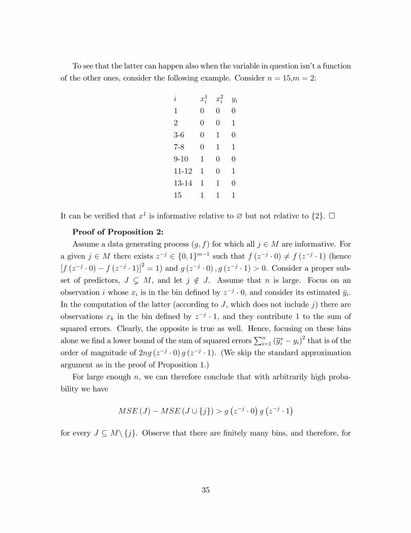
To see that the latter can happen also when the variable in question isn’t a function

of the other ones, consider the following example. Consider n = 15,m = 2:

i x1i x2i yi

1 0 0 0

2 0 0 1

3-6 0 1 0

7-8 0 1 1

9-10 1 0 0

11-12 1 0 1

13-14 1 1 0

15 1 1 1

It can be verified that x1 is informative relative to ∅ but not relative to {2}. �

Proof of Proposition 2:Assume a data generating process (g, f) for which all j ∈M are informative. For

a given j ∈ M there exists z−j ∈ {0, 1}m−1 such that f (z−j · 0) 6= f (z−j · 1) (hence

[f (z−j · 0)− f (z−j · 1)]2

= 1) and g (z−j · 0) , g (z−j · 1) > 0. Consider a proper sub-

set of predictors, J ( M , and let j /∈ J . Assume that n is large. Focus on an

observation i whose xi is in the bin defined by z−j · 0, and consider its estimated yi.In the computation of the latter (according to J , which does not include j) there are

observations xk in the bin defined by z−j · 1, and they contribute 1 to the sum of

squared errors. Clearly, the opposite is true as well. Hence, focusing on these bins

alone we find a lower bound of the sum of squared errors∑n

i=1 (ysi − yi)2 that is of the

order of magnitude of 2ng (z−j · 0) g (z−j · 1). (We skip the standard approximation

argument as in the proof of Proposition 1.)

For large enough n, we can therefore conclude that with arbitrarily high proba-

bility we have

MSE (J)−MSE (J ∪ {j}) > g(z−j · 0

)g(z−j · 1

)for every J ⊆ M\ {j}. Observe that there are finitely many bins, and therefore, for

35

a given δ > 0 one can find N such that for every n ≥ N

P

(MSE (J)−MSE (J ∪ {j}) > g (z−j · 0) g (z−j · 1)

∀j ∈M,∀J ⊆M\ {j}

)≥ 1− δ. (10)

We now turn to select a value c > 0 that would be small enough so that the

reduction in the AMSE thanks to omitting a variable j would not be worth the

increase due to the error. For each j, let

dj = max{g(z−j · 0

)g(z−j · 1

) ∣∣ z−j ∈ {0, 1}m−1 f(z−j · 0

)6= f

(z−j · 1

) }and

d ≡ minj∈M

dj.

Note that dj > 0 for all j (as each j is informative), and hence d > 0. Set c = d/2.

Given δ > 0 letN be such that for every n ≥ N (10) holds. Let c ∈ (0, c). We know

thatMSE (M) = 0 andAMSE (M) = mc. By the choice of c, arg minJ⊆M AMSE (J, c) =

{M}. Hence for any δ > 0 there exists N such that for every n ≥ N

P

(arg min

J⊆MAMSE (J, c) = {M}

)≥ 1− δ.

�

Proof of Proposition 3:As there are at least two observations with the value of yi = 0 and at least two

with yi = 1, if there is a variable j such that xji = yi (or xji = 1 − yi) for all i ≤ n,

the set J = {j} obtains MSE (J) = 0 (and AMSE (J) = c). We will show that the

proposition holds for J and J ′ that are (distinct) singletons.

Let the variables be generated according to the process described with 0 < η < 0.5.

Each xj has a probability of equalling y that is at least ηn. The probability it does not

provide a perfect fit is bounded above by (1− ηn) < 1 —which is a common bound

across all possible realizations of previously observed variables. The probability that

none of m such consecutively drawn variables provides a perfect fit is bounded above

by (1− ηn)m → 0 as m → ∞. Similarly if we consider m = 2k variables, and ask

what is the probability that there is at least one among the first k and at least one

among the second k such that each provides a perfect fit (xji = yi for all i) is at least

[1− (1− ηn)m]2 → 1 as m→∞. �

36

Proof of Theorem 1:Clearly, EMPIRICAL-SIMILARITY is in NP. Given a set of variable indices,

J ⊆M ≡ {1, ...,m}, computing its AMSE takes no more than O (n2m) steps.

The proof is by reduction of the SET-COVER problem to EMPIRICAL-SIMILARITY.

The former, which is known to be NPC (see Garey and Johnson, 1979), is defined as

Problem 3 SET-COVER: Given a set P , r ≥ 1 subsets thereof, T1, ..., Tr ⊆ P , and

an integer k (1 ≤ k ≤ r), are there k of the subsets that cover P? (That is, are there

indices 1 ≤ i1 ≤ i2 ≤ ... ≤ ik ≤ r such that ∪j≤kTij = P?)

Given an instance of SET-COVER, we construct, in polynomial time, an instance

of EMPIRICAL-SIMILARITY such that the former has a set cover iff the latter has

a similarity function that obtains the desired AMSE. Let there be given P , r ≥ 1

subsets thereof, T1, ..., Tr ⊆ P , and an integer k. Assume without loss of generality

that P = {1, ..., p}, that ∪i≤rTi = P , and that zuv ∈ {0, 1} is the incidence matrix ofthe subsets, that is, that for u ≤ p and v ≤ r, zuv = 1 iff u ∈ Tv.Let n = 2 (p+ 1) and m = r. Define the database B = {(xi, yi)}i≤n as follows.

(In the database each observation is repeated twice to avoid bins of size 1.)

For u ≤ p define two observations, i = 2u− 1, 2u by

xji = zuj yi = 1

and add two more observations, i = 2p+ 1, 2p+ 2 defined by

xji = 0 yi = 0.

Next, choose c to be such that 0 < c < 1mn3

, say, c = (mn3)−1/2 and R = kc. This

construction can obviously be done in polynomial time.

We claim that there is a cover of size k of P iff there is a similarity function defined

by a subset J ⊆ M ≡ {1, ...,m} such that AMSE(J, c) ≤ R. Let us begin with the

“only if” direction. Assume, then, that such a cover exists. Let J be the indices

1 ≤ i1 ≤ i2 ≤ ... ≤ ik ≤ r = m of the cover. For every i ≤ 2p, there exists j ∈ J suchthat xji = 1 and thus i is not in the same bin as 2p+1, 2p+2. It follows that for every

i′ such that swJ (xi, xi′) = 1 we have yi′ = yi = 1 and thus yswJi = 1 = yi. Similarly,

for i = 2p+ 1 and i′ = 2p+ 2 are similar only to each other and there we also obtain

perfect prediction: yswJi = 0 = yi. To conclude, SSE (J) = MSE (J) = 0. Thus,

37

AMSE(J, c) = MSE (J) + c |J | = ck = R.

Conversely, assume that J ⊆ M ≡ {1, ...,m} is such that AMSE(J, c) ≤ R.

We argue that we have to have SSE (J) = MSE (J) = 0. To see this, assume, to

the contrary, that J does not provide a perfect fit. Thus, there exists i such that

yswJi 6= yi. As yi ∈ {0, 1} and y

swJi is a relative frequency in a bin of size no greater

than n, the error∣∣yswJi − yi

∣∣ must be at least 1n. Therefore, SSE (J) ≥ 1

n2and

MSE (J) ≥ 1n3. However, R = ck ≤ cm and as c < 1

mn3as we have cm < 1

n3. Hence

MSE (J) ≥ 1n3> cm ≥ R, that is, MSE (J) > R and AMSE(J, c) > R follows, a

contradiction.

It follows that, if J obtains a low enough AMSE (AMSE(J, c) ≤ R), it obtains a

perfect fit. This is possible only if within each J-bin the values of yi’s are constant.

In particular, the observations i = 2p+ 1 and i′ = 2p+ 2 (which, being identical are

obviously in the same bin) are not similar to any other. That is, for every i ≤ 2p we

must have swJ (xi, x2p+1) = 0. This, in turn, means that for every such i there is a

j ∈ J such that xji 6= xj2p+1. But xj2p+1 = 0 so this means that xji = 1. Hence, for

every u ≤ p there is a j ∈ J such that xj2u = zuj = 1, that is, {Tv}v∈J is a cover of P .It only remains to note that AMSE(J, c) ≤ R implies that |J | ≤ k. �

Proof of Observation 2:Assume that m = 1, n = 4 and

i xi yi

1 0 0

2 1 0

3 3 1

4 4 1

In this example observations 1, 2 are closer to each other than each is to any of

observations 3, 4 and vice verse. (That is, |xi − xj| = 1 for i = 1, j = 2 as well as

for i = 3, j = 4, but |xi − xj| ≥ 2 for i ≤ 2 < j.) Moreover the values of y are the

same for the “close”observations and different for “distant”ones. (That is, yi = yj

for i = 1, j = 2 as well as for i = 3, j = 4, but |yi − yj| = 1 for i ≤ 2 < j.) If we

choose a finite w, the estimated value for each i, yswi , is a weighted average of the two

distant observations and the single close one. In particular, for every w <∞ we have

MSE (w) > 0.

38

Observe that w = w1 =∞ doesn’t provide a perfect fit either: if we set w = w1 =

∞, each observation i is considered to be dissimilar to any other, and its y value isestimated to be the default value, yswi = y0. Regardless of the (arbitrary) choice of

y0, the MSE is bounded below by that obtained for y = 0.5 (which is the average y

in the entire database). Thus, MSE (∞) ≥ 0.25.

Thus, MSE (w) > 0 for all w ∈ [0,∞]. However, as w → ∞ (but w < ∞),for each i the weight of the observation that is closest to i converges to 1 (and the

weights of the distant ones —to zero), so that yswi → yi. Hence, MSE (w)→w→∞ 0.

We thus conclude that infw∈[0,∞]MSE (w) = 0 but that there is no w that minimizes

the MSE. �

Proof of Proposition 4:We wish to show that arbitrarily low values of the MSE can be obtained with

probability that is arbitrarily close to 1. Let there be given ν > 0 and ξ > 0. We wish

to find N0 and W0 such that for every n ≥ N0, the vector w0 defined by wj0 = W0

satisfies

P (MSE (w0) < ν) ≥ 1− ξ.

To this end, we first wish to define “proximity”of the x values that would guarantee

“proximity”of the y values. Suppose that the latter is defined by ν/2. As the function

f is continuous on a compact set, it is uniformly continuous. Hence, there exists θ > 0

such that, for any x, x′ that satisfy ‖x− x′‖ < θ we have [f (x)− f (x′)]2 < ν/2. Let

us divide the set X into (4K√m/θ)

m equi-volume cubes, each with an edge of lengthθ

2√m. Two points x, x′ that belong to the same cube differ by at most θ

2√min each

coordinate and thus satisfy ‖x− x′‖ < θ/2. Let us now choose N1 such that, with

probability of at least (1− ξ/2), each such cube contains at least two observations xi(i ≤ N1). This guarantees that, when observation i is taken out of the sample, there

is another observation i′ (in the same cube), with [yi′ − f (xi)]2 < ν/2.

Next, we wish to bound the probability mass of each cube (defined by g). The

volume of a cube is(

θ2√m

)mand the density function is bounded from below by

η. Thus, the proportion of observations in the cube (out of all the n observations)

converges (as n→∞) to a number that is bounded from below by ζ ≡ η(

θ2√m

)m> 0.

Choose N0 ≥ N1 such that, with probability of at least (1− ξ/2), for each n ≥ N0

the proportion of the observations in the cube is at least ζ/2. Note that this is a

positive number which is independent of n.

39

Finally, we turn to choose W0. For each i, the proportion of observations xk with

[f (xi)− f (xk)]2 > ν is bounded above by (1− ζ). Define w0 by w

j0 = W0. Observe

that, as W0 →∞, ∑k 6=i,[f(xi)−f(xk)]2>ν s(xi, xk)∑k 6=i,[f(xi)−f(xk)]2≤ν s(xi, xk)

→ 0

and this convergence is uniform in n (as the definition of ζ is independent of n). Thus

a suffi ciently high W0 can be found so that, for all n ≥ N0, MSE (w0) < ν with

probability (1− ξ) or higher. �

Proof of Proposition 5:The general idea of the proof is very similar to that of Proposition 3: non-

uniqueness is obtained by showing that two variables can each provide perfect fit

on their own. In the continuous case, however, to obtain perfect fit one needs a bit

more than in the binary case: in the latter, it was suffi cient to assume that there are

at least two observations with yi = 0 and two with yi = 1; in the continuous case we

need to make sure that each yi has a close enough yk. For this reason, we state and

prove the result for a large n; yet, M (n) will be larger still, so that we should think

of this case as m >> n.

We now turn to prove the result formally. It will be convenient to define, for

w ∈ [0,∞]m, supp(w) ={l ∈M

∣∣wl > 0}.

Let there be given c > 0. Choose ε = c/3. We wish it to be the case that if

MSE (w) ≤ ε with #supp(w) = 1, then w ∈ ε-arg minAMSE, but for no w ∈ε-arg minAMSE is it the case that #supp(w) > 1. Clearly, the choice ε = c/3

guarantees that for every ε ∈ (0, ε), the second part of the claim holds: if a vector

w satisfies MSE (w) ≤ ε, no further reduction in the MSE can justify the cost of

additional variables, which is at least c. Conversely, because c < v/2 (the variance

of y), a single variable j that obtains a near-zero MSE would have a lower AMSE

than the empty set.

Let there now be given ε ∈ (0, ε) and every δ > 0. We need to find N and, for

every n ≥ N , M (n), such that for every n ≥ N and m ≥M (n),

P (ε- arg minAMSE is not connected) ≥ 1− δ.

40

Let N be large enough so that, with probability (1− δ/2), for all n ≥ N ,

maxi

mink 6=i

[yi − yj] < ε/2.

(To see that such an n can be found, one may divide the [−K,K] interval of values

to intervals of length ε/2 and choose N to be large enough so that, with the desired

probability, there are at least two observations in each such interval.)

Given such n ≥ N and the realizations of (yi)i≤n, consider the realizations of xj.

Assume that, for some j, it so happens that∣∣xji − yi∣∣ < ε/4 for all i ≤ n. In this

case, by setting wj to be suffi ciently high, and wl = 0 for l 6= j, one would obtain

MSE (w) ≤ ε and AMSE (w) ≤ ε + c.27 For each j, however, the probability that

this will be the case is bounded below by some ξ > 0, independent of n and j. Let

M1 (n) be a number such that, for any m ≥M1 (n), the probability that at least one

such j satisfies∣∣xji − yi∣∣ < ε/4 is (1− δ/4), and letM (n) > M1 (n) be a number such

that, for any m ≥ M (n), the probability that at least one more such j′ > j satisfies∣∣∣xj′i − yi∣∣∣ < ε/4 is (1− δ/8).

Thus, for every n ≥ N , and every m ≥ M (n), with probability 1 − δ there aretwo vectors, wj with support {j} and wj′ with support {j′}, each of which obtainingMSE (w) ≤ ε and thus, both belonging to ε-arg minAMSE. To see that in this

case the ε-arg minAMSE is not connected, it suffi ces to note that no w with support

greater than a singleton, nor a w with an empty support (that is, w ≡ 0) can be in

the ε-arg minAMSE. �

Proof of Theorem 2:We first verify that the problem is in NP. Given a database and a vector of

extended rational weights wj ∈ [0,∞], the calculation of the AMSE takes O (n2m)

steps as in the proof of Theorem 1. Specifically, the calculation of the similarity

function s (x, x′) is done by first checking whether there exists a j such that wj =∞and xj 6= x′j (in which case s (x, x′) is set to 0), and, if not —by ignoring the j’s for

which wj =∞.The proof that it is NPC is basically the same as that of Theorem 1, and we use the

same notation here. That is, we assume a given instance of SET-COVER: P , r ≥ 1

27The fact that xji is close to yi is immaterial, of course, as the variables xji are not used to predict

yi directly, but only to identify the yk that would. If xji is close to some monotone function of yi

the same argument would apply.

41

subsets thereof, T1, ..., Tr ⊆ P , and an integer k, with P = {1, ..., p}, ∪i≤rTi = P , and

the incidence matrix zuv ∈ {0, 1}. We let n = 2 (p+ 1) and m = r, and, for u ≤ p,

i = 2u − 1, 2u is given by xji = z′uj,yi = 1 whereas for i = 2p + 1, 2p + 2, xji = 0 and

yi = 0. We again set c = (mn3)−1/2 and R = kc. This construction can obviously

be done in polynomial time.

We claim that there exists a vector w with AMSE(w, c) ≤ R iff a cover of size k

exists for the given instance of SET-COVER.28 For the “if”part, assume that such a

cover exists, corresponding to J ⊆M . Setting the weights

wj =

{∞ j ∈ J0 j /∈ J

one obtains AMSE(w, c) ≤ R.

Conversely, for the “only if”part, assume that a vector of rational weights w =

(wj)j (wj ∈ [0,∞]) obtains AMSE(w, c) ≤ R. Let J ⊆ M be the set of indices of

predictors that have a positive wj (∞ included). By the definition of R (as equal to

ck), it has to be the case that |J | ≤ k. We argue that J defines a cover (that is, that

{Tv}v∈J is a cover of P ).Observe that, if we knew that |J | = k, the inequality

AMSE(w, c) = MSE (w) + c |J | ≤ R = ck

could only hold ifMSE (w) = 0, from which it would follow that w provides a perfect

fit. In particular, for every i ≤ 2p there exists j ∈ J such that xji 6= xj2p+1 that is,

xji = 1, and J defines a cover of P .

However, it is still possible that |J | < k and 0 < MSE (w) ≤ c (k − |J |). Yet, evenin this case, J defines a cover. To see this, assume that this is not the case. Then, as

in the proof of Theorem 1, there exists i ≤ 2p such that for all j, either wj = 0 (j /∈ J)or xji = 0 = xj2p+1. This means that s (xi, x2p+1) = s (xi, x2p+2) = 1. In particular,

y2p+1 = y2p+2 = 0 take part (with positive weights) in the computation of yswi and we

have yswi < 1 = yi. In the proof of Theorem 1 this suffi ced to bound the error |yswi − yi|from below by 1

n, as all observations with positive weights had the same weights. This

28This proof uses values of x and of y that are in {0, 1}. However, if we consider the same problemin which the input is restricted to be positive-length ranges of the variables, one can prove a similarresult with suffi ciently small ranges and a value of R that is accordingly adjusted.

42

is no longer the case here. However, the cases 2p+1, 2p+2 obtain maximal similarity

to i (s (xi, x2p+1) = s (xi, x2p+2) = 1), because xj2p+1 = xj2p+2 = xji (= 0) for all j with

wj > 0. (It is possible that for other observations l ≤ 2p we have s (xi, x2p+1) ∈ (0, 1),

which was ruled out in the binary case. But the weights of these observations are

evidently smaller than that of 2p+ 1, 2p+ 2.) Thus we obtain (again) that the error

|yswi − yi| must be at least 1n, from which SSE (w) ≥ 1

n2and MSE (w) ≥ 1

n3follow.

This implies AMSE(w, c) > R and concludes the proof. �

References

[1] Akaike, H. (1954), “An Approximation to the Density Function”, Annals of the

Institute of Statistical Mathematics, 6: 127-132.

[2] Akaike, H. (1974), “A New Look at the Statistical Model Identification”. IEEE

Transactions on Automatic Control 19 (6), 716—723.

[3] Anscombe, F. J. and R. J. Aumann (1963), “A Definition of Subjective Proba-

bility”, The Annals of Mathematics and Statistics, 34: 199-205.

[4] Aragones, E., I. Gilboa, A. Postlewaite, and D. Schmeidler (2005), “Fact-Free

Learning”, American Economic Review, 95: 1355-1368.

[5] Argenziano, R. and I. Gilboa (2012), “History as a Coordination Device”, Theory

and Decision, 73: 501-512.

[6] Argenziano, R. and I. Gilboa (2018), “Learning What is Similar: Precedents and

Equilibrium Selection”, working paper.

[7] Aumann, R. J. (1976), “Agreeing to Disagree”, The Annals of Statistics, 4:1236-1239.

[8] Aumann, R. J. (1987), “Correlated Equilibrium as an Expression of Bayesian

Rationality”, Econometrica, 55: 1-18.

43

[9] Billot, A., I. Gilboa, D. Samet, and D. Schmeidler (2005), “Probabilities as

Similarity-Weighted Frequencies”, Econometrica, 73: 1125-1136.

[10] Billot, A., I. Gilboa, and D. Schmeidler (2008), “Axiomatization of an Exponen-

tial Similarity Function”, Mathematical Social Sciences, 55: 107-115.

[11] Brandenburger, A. and E. Dekel (1987), “Rationalizability and Correlated Equi-

libria”, Econometrica, 55: 1391-1402.

[12] Bray, M. (1982), “Learning, Estimation, and the Stability of Rational Expecta-

tions”, Journal of Economic Theory, 26: 318-339.

[13] Cortes, C., and V. Vapnik (1995), “Support-Vector Networks”, Machine Learn-

ing, 20: 273-297.

[14] de Finetti, B. (1931), Sul Significato Soggettivo della Probabilità, Fundamenta

Mathematicae, 17: 298-329.

[15] – – – —(1937), “La Prevision: ses Lois Logiques, ses Sources Subjectives”, An-

nales de l’Institut Henri Poincare, 7: 1-68.

[16] Eilat, R. (2007), “Computational Tractability of Searching for Optimal Regular-

ities”, working paper.

[17] Fix, E. and J. Hodges (1951), “Discriminatory Analysis. Nonparametric Dis-

crimination: Consistency Properties”. Technical Report 4, Project Number 21-

49-004, USAF School of Aviation Medicine, Randolph Field, TX.

[18] – – – —(1952), ”Discriminatory Analysis: Small Sample Performance”. Tech-

nical Report 21-49-004, USAF School of Aviation Medicine, Randolph Field,

TX.

[19] Gilboa, I. and D. Schmeidler (1995), “Case-Based Decision Theory”, The Quar-

terly Journal of Economics, 110: 605-639.

44

[20] – – – —(2001), A Theory of Case-Based Decisions, Cambridge: Cambridge Uni-

versity Press.

[21] – – – —(2012), Case-Based Predictions. World Scientific Publishers, Economic

Theory Series (Eric Maskin, Ed.), 2012.

[22] Gilboa, I., O. Lieberman, and D. Schmeidler (2006), “Empirical Similarity”,

Review of Economics and Statistics, 88: 433-444.

[23] Gul, F. (1998), “A Comment on Aumann’s Bayesian View”, Econometrica, 66:923-928.

[24] Hume, D. (1748), An Enquiry Concerning Human Understanding. Oxford:

Clarendon Press.

[25] Jaekel, F., B. Schoelkopf, and F. A. Wichmann (2008), “Generalization and Sim-

ilarity in Exemplar Models of Categorization: Insights from Machine Learning”,

Psychonomic Bulletin & Review, 15: 256-271.

[26] – – – —(2009), “Does Cognitive Science Need Kernels?”, Trends in Cognitive

Sciences, 13: 381-388.

[27] Kohavi, R. (1995), “A Study of Cross-Validation and Bootstrap for Accuracy

Estimation and Model Selection”, Proceedings of the International Joint Confer-

ence on Artificial Intelligence.

[28] Lieberman, O. (2010), “Asymptotic Theory for Empirical Similarity Models”,

Econometric Theory, 26: 1032-1059.

[29] – – – —(2012), “A Similarity-Based Approach to Time-Varying Coeffi cient Non-

stationary Autoregression”, Journal of Time Series Analysis, 33: 484-502.

[30] Lieberman, O. and P. F. Phillips (2014), “Norming Rates and Limit Theory

for Some Time-Varying Coeffi cient Autoregressions”, Journal of Time Series

Analysis, 35: 592-623.

45

[31] – – – —(2017), “AMultivariate Stochastic Unit Root Model with an Application

to Derivative Pricing”, Journal of Econometrics, 196: 99-110.

[32] Medin. D. L. andM. M. Schaffer (1978), “Context Theory of Classification Learn-

ing”, Psychological Review, 85: 207-238.

[33] Morris, S. (1995), “The Common Prior Assumption in Economic Theory”, Eco-

nomics and Philosophy, 11: 227-253.

[34] Nadaraya, E. A. (1964), “On Estimating Regression”, Theory of Probability and

its Applications, 9: 141—142.

[35] Nosofsky, R. M. (1984), “Choice, Similarity, and the Context Theory of Classifi-

cation”, Journal of Experimental Psychology: Learning, Memory, and Cognition,

10: 104-114.

[36] – – – —(1988), “Exemplar-Based Accounts of Relations Between Classification,

Recognition, and Typicality”, Journal of Experimental Psychology: Learning,

Memory, and Cognition, 14: 700-708.

[37] – – – —(2014), “The Generalized Context Model: An Exemplar Model of Clas-

sification”, in Formal Approaches in Categorization, Cambridge University Press,

New York, Chapter 2, 18-39.

[38] Park, B. U. and Marron, J. S. (1990), “Comparison of data-driven bandwidth

selectors”, Journal of the American Statistical Association, 85: 66—72.

[39] Parzen, E. (1962), “On the Estimation of a Probability Density Function and

the Mode”, Annals of Mathematical Statistics, 33: 1065-1076.

[40] Ramsey, F. P. (1926), “Truth and Probability”, in R. Braithwaite (ed.), (1931),

The Foundation of Mathematics and Other Logical Essays. London: Routledge

and Kegan.

[41] Rosenblatt, M. (1956), “Remarks on Some Nonparametric Estimates of a Density

Function”, Annals of Mathematical Statistics, 27: 832-837.

46

[42] Savage, L. J. (1954), The Foundations of Statistics. New York: John Wiley and

Sons. (Second addition in 1972, Dover)

[43] Scott, D. W. (1992), Multivariate Density Estimation: Theory, Practice, and

Visualization. New York: John Wiley and Sons.

[44] Shepard, R. N. (1957), “Stimulus and Response Generalization: A Stochastic

Model Relating Generalization to Distance in Psychological Space”, Psychome-

trika, 22: 325-345

[45] – – – —(1987), “Towards a Universal Law of Generalization for Psychological

Science”, Science, 237: 1317-1323

[46] Silverman, B. W. (1986), Density Estimation for Statistics and Data Analysis.

London and New York: Chapman and Hall.

[47] Steiner, J., and C. Stewart, C. (2008), “Contagion through Learning”, Theoret-

ical Economics, 3: 431-458.

[48] Vapnik, V. (1998), Statistical Learning Theory, New York: John Wiley and Sons.

[49] – – – —(2000), The Nature of Statistical Learning Theory, Berlin: Springer.

[50] Watson, G. S. (1964), “Smooth regression analysis”, Sankhya: The Indian Jour-

nal of Statistics, Series A, 26: 359—372.

[51] Wittgenstein, L. (1922), Tractatus Logico Philosophicus. London: Routledge and

Kegan Paul.

47