Secret and joy of configurational mechanics: From foundations in continuum mechanics to applications in computational mechanics

ZAMM · Z. Angew. Math. Mech. 89, No. 8, 614 – 630 (2009) / DOI 10.1002/zamm.200800132

Secret and joy of configurational mechanics: From foundations incontinuum mechanics to applications in computational mechanics

Paul Steinmann1,∗, Michael Scherer1, and Ralf Denzer2

1 Chair of Applied Mechanics, University of Erlangen-Nuremberg, Egerlandstr. 5, 91058 Erlangen, Germany2 Department of Mechanical and Structural Engineering, University of Trento, Via Mesiano 77, 38100 Trento, Italy

Received 13 August 2008, accepted 5 November 2008Published online 20 February 2009

Key words Configurational mechanics, computational mechanics.

This manuscript contains the material presented in a plenary lecture given at the GAMM annual meeting 2007 in Zurich

Over the recent years configurational mechanics has developed into a very active and successful topic both in continuummechanics as well as in computational mechanics. On the continuum mechanics side the basic idea is to consider energyvariations that go along with changes of the material configuration. Configurational forces are then energetically dual tothese configurational changes. Configurational forces take the interpretation as being the driving forces in the kinetics ofdefects; like e.g., cracks, inclusions, phase boundaries, dislocations and the like. On the computational side it turns out thata discretisation scheme brings in artificial, discrete configurational forces that indicate in a certain sense the quality, e.g., ofa finite-element mesh. This information can then be used to optimize the nodal material positions. Surprisingly, even drivenby energetical arguments, it turns out that a finite element mesh optimized with respect to discrete configurational forcesalso renders superior results in terms of classical error measures. The manuscript will span the field from the underlyingtheoretical foundations over the algorithmic challenges to various computational applications.

c© 2009 WILEY-VCH Verlag GmbH & Co. KGaA, Weinheim

1 Introduction

Classical (deformational) continuum mechanics deals with the response of a continuum body to externally prescribedloading such as, e.g., distributed body forces, boundary tractions, and boundary displacements. We thus typically askfor the placement in the spatial (current) configuration into which each continuum point is mapped due to the action ofthis external loading. Configurational mechanics, however, is concerned with the energetic changes that go along with avariation of the material (initial) configuration, in short with configurational changes. A possible energy release could thenbe re-invested into other physical processes like, e.g., the creation of new surfaces or the material motion of defects.

Configurational mechanics is a rather active field: comprehensive overviews that discuss various theoretical aspects ofconfigurational mechanics can be found, e.g., in [11–13,15,16]. Many recent impressive developments are in the applicationof concepts from configurational mechanics to computational mechanics, see, e.g., [17–22,31]. Our own contributions to thefield are, e.g., [1, 2, 4, 6, 14,23–30, 32]. In this contribution we will give an overview on different aspects of configurationalmechanics from the foundations in continuum mechanics to various applications in computational mechanics.

2 Secret of configurational mechanics

A continuum body occupies initially the material configurationB0 with continuum points labelled by the material placementX and deforms due to prescribed loading into the spatial configuration Bt with continuum points labelled by the spatialplacement x. A spatial deformation is a mapping x = ϕ(X) and a material deformation is a mapping X = Φ(x) withΦ = ϕ−1. This section elaborates on the relation between the localized force balance in spatial and material description.Here the terminology spatial or material description refers to fields expressed in a tangent space to either the spatial orthe material configuration. It will turn out that four different localized force balances can be established that can easily betransformed into each other by pull-back and push-forward operations in terms of the deformation gradients F = ∇Xϕand f = ∇xΦ with f = F−1, see [27]. Here ∇X and ∇x denote the gradient operators with respect to the materialcoordinates X and the spatial coordinates x, respectively.

∗ Corresponding author E-mail: [email protected], Phone: +49 9131 85 28501, Fax: +49 9131 85 28503

c© 2009 WILEY-VCH Verlag GmbH & Co. KGaA, Weinheim

ZAMM · Z. Angew. Math. Mech. 89, No. 8 (2009) / www.zamm-journal.org 615

2.1 Localized force balance in spatial description

The (ordinary) force balance in spatial description requires the spatial contact and body forces acting on a body to be inequilibrium. The localization of this elementary statement renders with the help of the Cauchy theorem for the spatialtraction t0 = P · N (N denotes the material outward unit normal to the boundary ∂B0) with material reference (contactforce per unit area in the material configuration) the well known expression

DivP + b0 = 0. (1)

Here P denotes the two-point Piola stress, b0 is the spatial body force density with material reference (e.g. gravityacting on a unit volume in the material configuration) and Div is the divergence operator with respect to the materialcoordinates X . Within a conservative setting, that we shall assume for the sake of simplicity, the Piola stress P and thebody force density b0 are derived from a total potential energy density U0 = U0(ϕ, F ; X) per unit volume in the materialconfiguration

P := ∂F U0, b0 := −∂ϕU0. (2)

Here the total potential energy density U0 is composed of an external and an internal contribution U0 = V0(ϕ; X) +W0(F ; X). The localized force balance in spatial description may alternatively be expressed in terms of the Cauchy stressσ and the spatial body force density bt with spatial reference (i.e. per unit volume in the spatial configuration)

divσ + bt = 0. (3)

Here div denotes the divergence operator with respect to the spatial coordinates x. The Cauchy stress σ is the Piolatransform of the Piola stress P , thus incorporating the constitutive law in Eq. (2) with U0 = JUt, J = detF and j = J−1

renders a particular structure for the Cauchy stress that might be denoted as energy-momentum format

σ := jP · F t = Uti − f t · ∂f Ut bt := −∂ϕUt. (4)

In the above i denotes as usual the spatial unit tensor.

2.2 Localized force balance in material description

In analogy to the force balance in spatial description we may, for the time being only formally, postulate a force balancein material description. The localization of this formal statement renders with the help of a Cauchy-type theorem for thematerial traction T t = p · n with spatial reference (n denotes the spatial outward unit normal to the boundary ∂Bt)

divp + Bt = 0. (5)

Here p denotes a new, however yet unspecified two-point stress and Bt is a material body force density with spatialreference. Again for analogy the two-point stress p and the body force density Bt are derived within a conservative settingfrom the total potential energy density Ut = Ut(Φ, f ; x) per unit volume in the spatial configuration (Ut = jU0, j =detf ), whereby now the role of the material X → Φ and spatial ϕ → x placement as either parameter or field arereversed (note that f = F−1 is clearly a function of F )

p := ∂fUt, Bt := −∂ΦUt. (6)

The localized force balance in material description may alternatively be expressed in terms of the Eshelby stress Σ andthe material body force density B0 with material reference

DivΣ + B0 = 0. (7)

Thereby the Eshelby stress Σ is the Piola transform of p, thus incorporating the constitutive law in Eq. (6) renders aparticular structure for the Eshelby stress that is commonly denoted as energy-momentum format

Σ := Jp · f t = U0I − F t · ∂F U0, B0 := −∂ΦU0. (8)

In the above I denotes the material unit tensor.

www.zamm-journal.org c© 2009 WILEY-VCH Verlag GmbH & Co. KGaA, Weinheim

616 P. Steinmann et al.: Configurational mechanics

2.3 Spatial versus material description

Based on the constitutive laws in Eqs. (2), (6) and the energy-momentum format for the Eshelby and the Cauchy stress,Σ and σ, it turns out that the localized force balances in spatial and material description are directly related by push-forward/pull-back operations in terms of the deformation gradients F and f

F t · [DivP + b0] = 0 → DivΣ + B0 = 0 and f t · [divp + Bt] = 0 → divσ + bt = 0. (9)

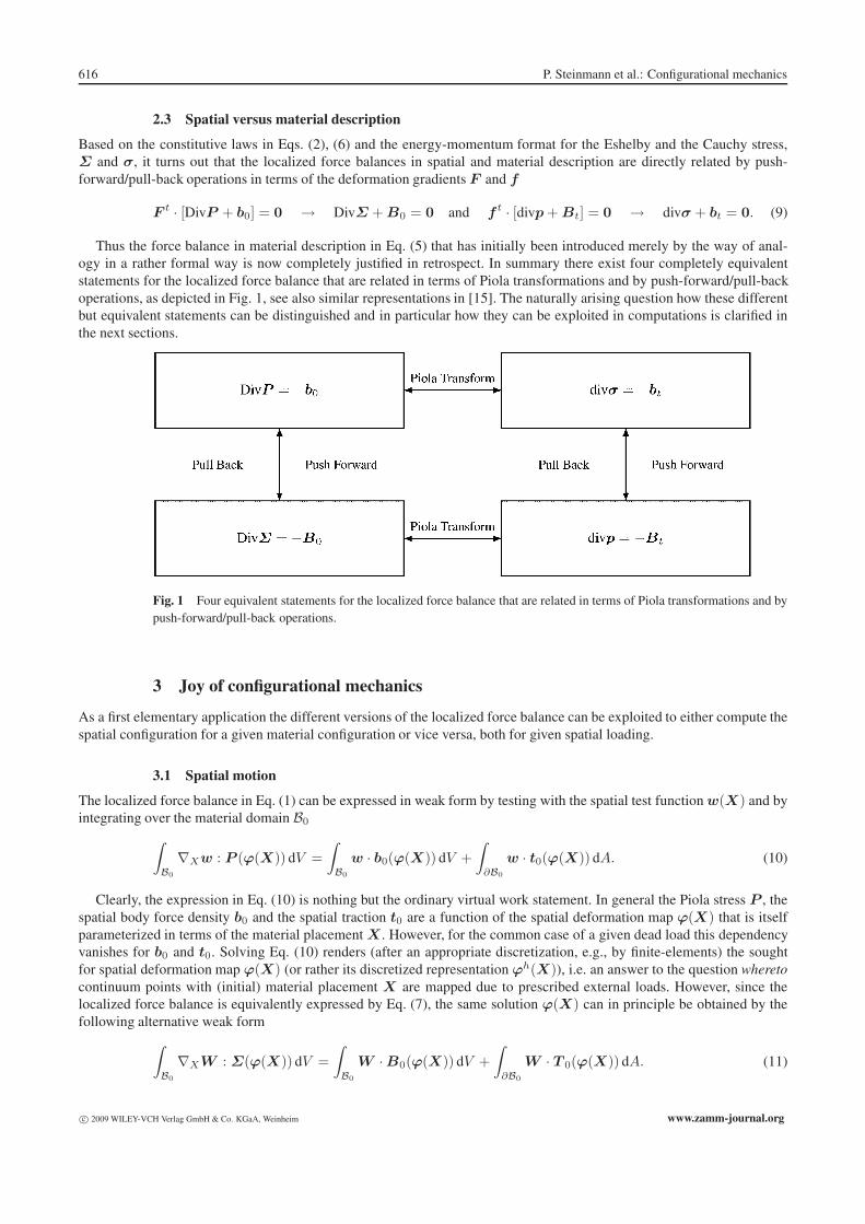
Thus the force balance in material description in Eq. (5) that has initially been introduced merely by the way of anal-ogy in a rather formal way is now completely justified in retrospect. In summary there exist four completely equivalentstatements for the localized force balance that are related in terms of Piola transformations and by push-forward/pull-backoperations, as depicted in Fig. 1, see also similar representations in [15]. The naturally arising question how these differentbut equivalent statements can be distinguished and in particular how they can be exploited in computations is clarified inthe next sections.

Fig. 1 Four equivalent statements for the localized force balance that are related in terms of Piola transformations and bypush-forward/pull-back operations.

3 Joy of configurational mechanics

As a first elementary application the different versions of the localized force balance can be exploited to either compute thespatial configuration for a given material configuration or vice versa, both for given spatial loading.

3.1 Spatial motion

The localized force balance in Eq. (1) can be expressed in weak form by testing with the spatial test function w(X) and byintegrating over the material domain B0

∫B0

∇Xw : P (ϕ(X)) dV =∫B0

w · b0(ϕ(X)) dV +∫

∂B0

w · t0(ϕ(X)) dA. (10)

Clearly, the expression in Eq. (10) is nothing but the ordinary virtual work statement. In general the Piola stress P , thespatial body force density b0 and the spatial traction t0 are a function of the spatial deformation map ϕ(X) that is itselfparameterized in terms of the material placement X . However, for the common case of a given dead load this dependencyvanishes for b0 and t0. Solving Eq. (10) renders (after an appropriate discretization, e.g., by finite-elements) the soughtfor spatial deformation map ϕ(X) (or rather its discretized representation ϕh(X)), i.e. an answer to the question wheretocontinuum points with (initial) material placement X are mapped due to prescribed external loads. However, since thelocalized force balance is equivalently expressed by Eq. (7), the same solution ϕ(X) can in principle be obtained by thefollowing alternative weak form

∫B0

∇XW : Σ(ϕ(X)) dV =∫B0

W · B0(ϕ(X)) dV +∫

∂B0

W · T 0(ϕ(X)) dA. (11)

c© 2009 WILEY-VCH Verlag GmbH & Co. KGaA, Weinheim www.zamm-journal.org


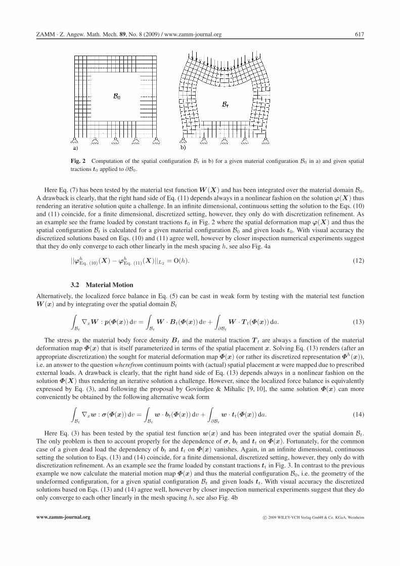
Fig. 2 Computation of the spatial configuration Bt in b) for a given material configuration B0 in a) and given spatialtractions t0 applied to ∂B0.

Here Eq. (7) has been tested by the material test function W (X) and has been integrated over the material domain B0.A drawback is clearly, that the right hand side of Eq. (11) depends always in a nonlinear fashion on the solution ϕ(X) thusrendering an iterative solution quite a challenge. In an infinite dimensional, continuous setting the solution to the Eqs. (10)and (11) coincide, for a finite dimensional, discretized setting, however, they only do with discretization refinement. Asan example see the frame loaded by constant tractions t0 in Fig. 2 where the spatial deformation map ϕ(X) and thus thespatial configuration Bt is calculated for a given material configuration B0 and given loads t0. With visual accuracy thediscretized solutions based on Eqs. (10) and (11) agree well, however by closer inspection numerical experiments suggestthat they do only converge to each other linearly in the mesh spacing h, see also Fig. 4a

||ϕhEq. (10)(X) − ϕh

Eq. (11)(X)||L2 = O(h). (12)

3.2 Material Motion

Alternatively, the localized force balance in Eq. (5) can be cast in weak form by testing with the material test functionW (x) and by integrating over the spatial domain Bt

∫Bt

∇xW : p(Φ(x)) dv =∫Bt

W · Bt(Φ(x)) dv +∫

∂Bt

W · T t(Φ(x)) da. (13)

The stress p, the material body force density Bt and the material traction T t are always a function of the materialdeformation map Φ(x) that is itself parameterized in terms of the spatial placement x. Solving Eq. (13) renders (after anappropriate discretization) the sought for material deformation map Φ(x) (or rather its discretized representation Φh(x)),i.e. an answer to the question wherefrom continuum points with (actual) spatial placement x were mapped due to prescribedexternal loads. A drawback is clearly, that the right hand side of Eq. (13) depends always in a nonlinear fashion on thesolution Φ(X) thus rendering an iterative solution a challenge. However, since the localized force balance is equivalentlyexpressed by Eq. (3), and following the proposal by Govindjee & Mihalic [9, 10], the same solution Φ(x) can moreconveniently be obtained by the following alternative weak form

∫Bt

∇xw : σ(Φ(x)) dv =∫Bt

w · bt(Φ(x)) dv +∫

∂Bt

w · tt(Φ(x)) da. (14)

Here Eq. (3) has been tested by the spatial test function w(x) and has been integrated over the spatial domain Bt.The only problem is then to account properly for the dependence of σ, bt and tt on Φ(x). Fortunately, for the commoncase of a given dead load the dependency of bt and tt on Φ(x) vanishes. Again, in an infinite dimensional, continuoussetting the solution to Eqs. (13) and (14) coincide, for a finite dimensional, discretized setting, however, they only do withdiscretization refinement. As an example see the frame loaded by constant tractions tt in Fig. 3. In contrast to the previousexample we now calculate the material motion map Φ(x) and thus the material configuration B0, i.e. the geometry of theundeformed configuration, for a given spatial configuration Bt and given loads tt. With visual accuracy the discretizedsolutions based on Eqs. (13) and (14) agree well, however by closer inspection numerical experiments suggest that they doonly converge to each other linearly in the mesh spacing h, see also Fig. 4b



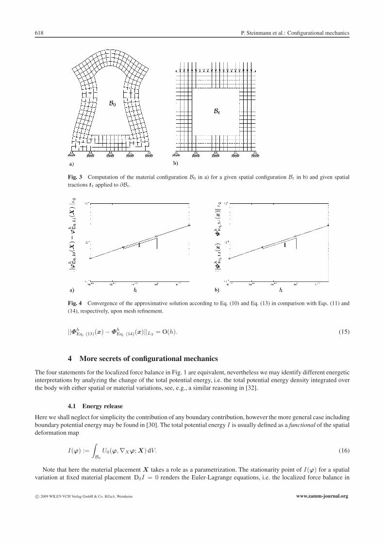
Fig. 3 Computation of the material configuration B0 in a) for a given spatial configuration Bt in b) and given spatialtractions tt applied to ∂Bt.

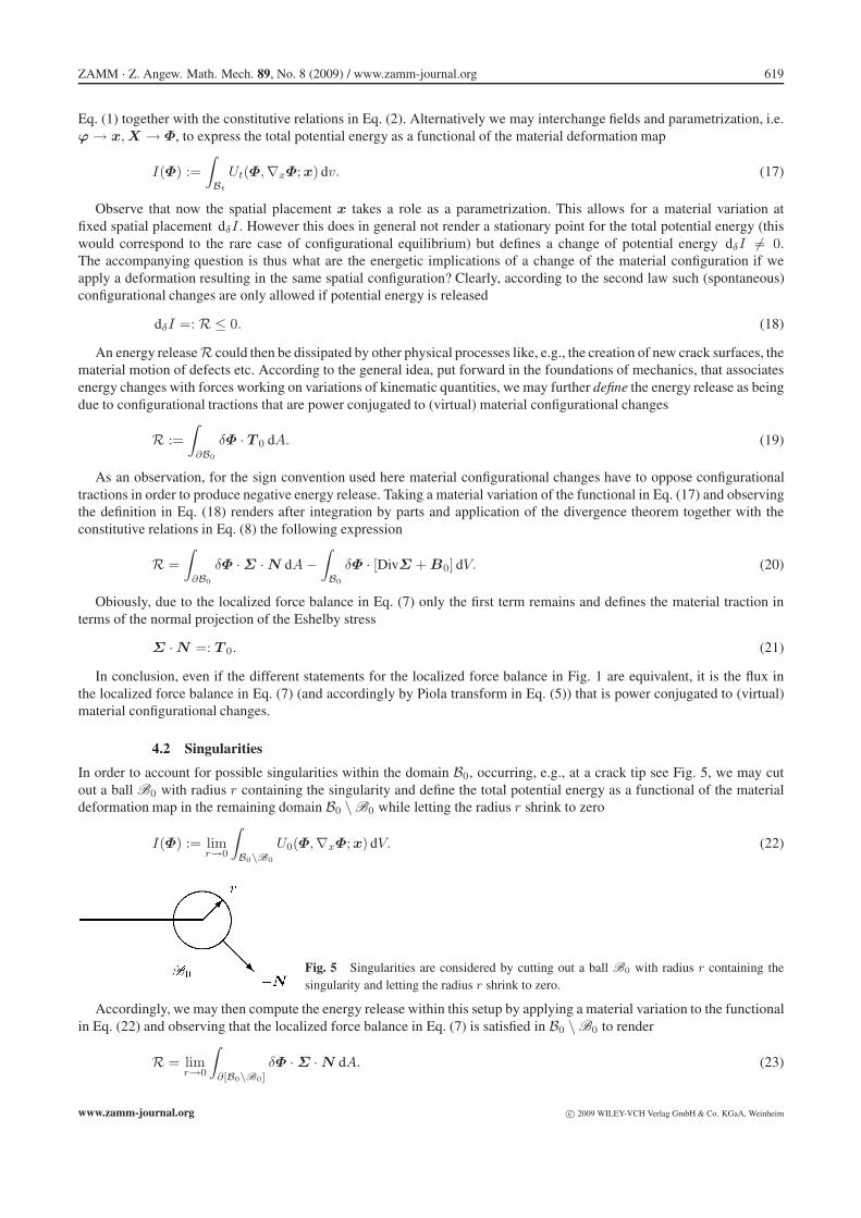
Fig. 4 Convergence of the approximative solution according to Eq. (10) and Eq. (13) in comparison with Eqs. (11) and(14), respectively, upon mesh refinement.

||ΦhEq. (13)(x) − Φh

Eq. (14)(x)||L2 = O(h). (15)

4 More secrets of configurational mechanics

The four statements for the localized force balance in Fig. 1 are equivalent, nevertheless we may identify different energeticinterpretations by analyzing the change of the total potential energy, i.e. the total potential energy density integrated overthe body with either spatial or material variations, see, e.g., a similar reasoning in [32].

4.1 Energy release

Here we shall neglect for simplicity the contribution of any boundary contribution, however the more general case includingboundary potential energy may be found in [30]. The total potential energy I is usually defined as a functional of the spatialdeformation map

I(ϕ) :=∫B0

U0(ϕ,∇Xϕ; X) dV. (16)

Note that here the material placement X takes a role as a parametrization. The stationarity point of I(ϕ) for a spatialvariation at fixed material placement DδI = 0 renders the Euler-Lagrange equations, i.e. the localized force balance in



Eq. (1) together with the constitutive relations in Eq. (2). Alternatively we may interchange fields and parametrization, i.e.ϕ → x, X → Φ, to express the total potential energy as a functional of the material deformation map

I(Φ) :=∫Bt

Ut(Φ,∇xΦ; x) dv. (17)

Observe that now the spatial placement x takes a role as a parametrization. This allows for a material variation atfixed spatial placement dδI . However this does in general not render a stationary point for the total potential energy (thiswould correspond to the rare case of configurational equilibrium) but defines a change of potential energy dδI �= 0.The accompanying question is thus what are the energetic implications of a change of the material configuration if weapply a deformation resulting in the same spatial configuration? Clearly, according to the second law such (spontaneous)configurational changes are only allowed if potential energy is released

dδI =: R ≤ 0. (18)

An energy release R could then be dissipated by other physical processes like, e.g., the creation of new crack surfaces, thematerial motion of defects etc. According to the general idea, put forward in the foundations of mechanics, that associatesenergy changes with forces working on variations of kinematic quantities, we may further define the energy release as beingdue to configurational tractions that are power conjugated to (virtual) material configurational changes

R :=∫

∂B0

δΦ · T 0 dA. (19)

As an observation, for the sign convention used here material configurational changes have to oppose configurationaltractions in order to produce negative energy release. Taking a material variation of the functional in Eq. (17) and observingthe definition in Eq. (18) renders after integration by parts and application of the divergence theorem together with theconstitutive relations in Eq. (8) the following expression

R =∫

∂B0

δΦ · Σ · N dA −∫B0

δΦ · [DivΣ + B0] dV. (20)

Obiously, due to the localized force balance in Eq. (7) only the first term remains and defines the material traction interms of the normal projection of the Eshelby stress

Σ · N =: T 0. (21)

In conclusion, even if the different statements for the localized force balance in Fig. 1 are equivalent, it is the flux inthe localized force balance in Eq. (7) (and accordingly by Piola transform in Eq. (5)) that is power conjugated to (virtual)material configurational changes.

4.2 Singularities

In order to account for possible singularities within the domain B0, occurring, e.g., at a crack tip see Fig. 5, we may cutout a ball B0 with radius r containing the singularity and define the total potential energy as a functional of the materialdeformation map in the remaining domain B0 \ B0 while letting the radius r shrink to zero

I(Φ) := limr→0

∫B0\B0

U0(Φ,∇xΦ; x) dV. (22)

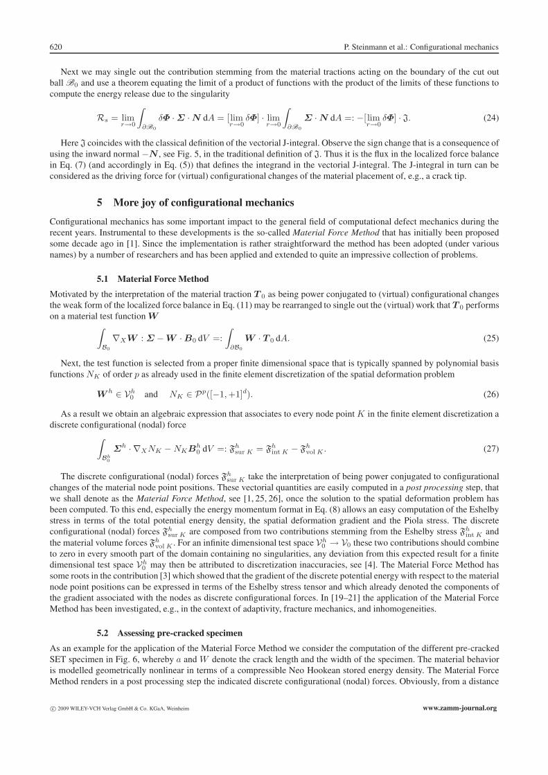
Fig. 5 Singularities are considered by cutting out a ball B0 with radius r containing thesingularity and letting the radius r shrink to zero.

Accordingly, we may then compute the energy release within this setup by applying a material variation to the functionalin Eq. (22) and observing that the localized force balance in Eq. (7) is satisfied in B0 \ B0 to render

R = limr→0

∫∂[B0\B0]

δΦ · Σ · N dA. (23)



Next we may single out the contribution stemming from the material tractions acting on the boundary of the cut outball B0 and use a theorem equating the limit of a product of functions with the product of the limits of these functions tocompute the energy release due to the singularity

Rs = limr→0

∫∂B0

δΦ · Σ · N dA = [limr→0

δΦ] · limr→0

∫∂B0

Σ · N dA =: −[ limr→0

δΦ] · J. (24)

Here J coincides with the classical definition of the vectorial J-integral. Observe the sign change that is a consequence ofusing the inward normal −N , see Fig. 5, in the traditional definition of J. Thus it is the flux in the localized force balancein Eq. (7) (and accordingly in Eq. (5)) that defines the integrand in the vectorial J-integral. The J-integral in turn can beconsidered as the driving force for (virtual) configurational changes of the material placement of, e.g., a crack tip.

5 More joy of configurational mechanics

Configurational mechanics has some important impact to the general field of computational defect mechanics during therecent years. Instrumental to these developments is the so-called Material Force Method that has initially been proposedsome decade ago in [1]. Since the implementation is rather straightforward the method has been adopted (under variousnames) by a number of researchers and has been applied and extended to quite an impressive collection of problems.

5.1 Material Force Method

Motivated by the interpretation of the material traction T 0 as being power conjugated to (virtual) configurational changesthe weak form of the localized force balance in Eq. (11) may be rearranged to single out the (virtual) work that T 0 performson a material test function W∫

B0

∇XW : Σ − W · B0 dV =:∫

∂B0

W · T 0 dA. (25)

Next, the test function is selected from a proper finite dimensional space that is typically spanned by polynomial basisfunctions NK of order p as already used in the finite element discretization of the spatial deformation problem

W h ∈ Vh0 and NK ∈ Pp([−1, +1]d). (26)

As a result we obtain an algebraic expression that associates to every node point K in the finite element discretization adiscrete configurational (nodal) force

∫Bh

0

Σh · ∇XNK − NKBh0 dV =: Fh

sur K = Fhint K − Fh

vol K . (27)

The discrete configurational (nodal) forces Fhsur K take the interpretation of being power conjugated to configurational

changes of the material node point positions. These vectorial quantities are easily computed in a post processing step, thatwe shall denote as the Material Force Method, see [1, 25, 26], once the solution to the spatial deformation problem hasbeen computed. To this end, especially the energy momentum format in Eq. (8) allows an easy computation of the Eshelbystress in terms of the total potential energy density, the spatial deformation gradient and the Piola stress. The discreteconfigurational (nodal) forces Fh

sur K are composed from two contributions stemming from the Eshelby stress Fhint K and

the material volume forces Fhvol K . For an infinite dimensional test space Vh

0 → V0 these two contributions should combineto zero in every smooth part of the domain containing no singularities, any deviation from this expected result for a finitedimensional test space Vh

0 may then be attributed to discretization inaccuracies, see [4]. The Material Force Method hassome roots in the contribution [3] which showed that the gradient of the discrete potential energy with respect to the materialnode point positions can be expressed in terms of the Eshelby stress tensor and which already denoted the components ofthe gradient associated with the nodes as discrete configurational forces. In [19–21] the application of the Material ForceMethod has been investigated, e.g., in the context of adaptivity, fracture mechanics, and inhomogeneities.

5.2 Assessing pre-cracked specimen

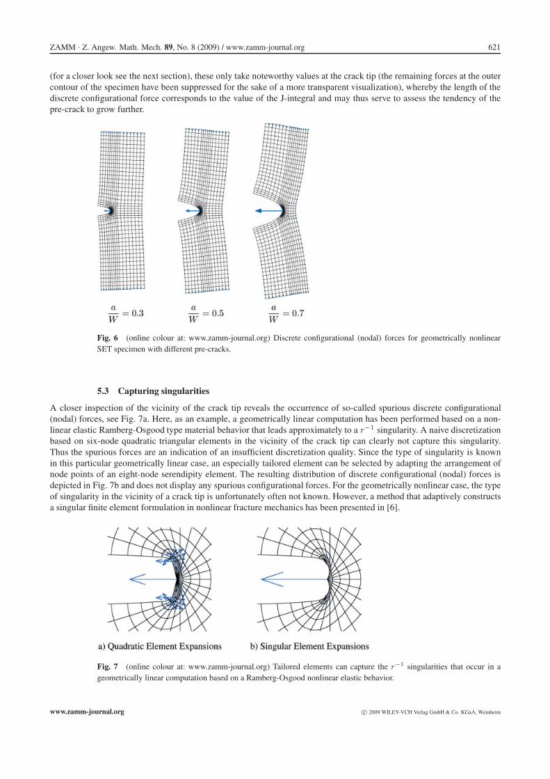
As an example for the application of the Material Force Method we consider the computation of the different pre-crackedSET specimen in Fig. 6, whereby a and W denote the crack length and the width of the specimen. The material behavioris modelled geometrically nonlinear in terms of a compressible Neo Hookean stored energy density. The Material ForceMethod renders in a post processing step the indicated discrete configurational (nodal) forces. Obviously, from a distance



(for a closer look see the next section), these only take noteworthy values at the crack tip (the remaining forces at the outercontour of the specimen have been suppressed for the sake of a more transparent visualization), whereby the length of thediscrete configurational force corresponds to the value of the J-integral and may thus serve to assess the tendency of thepre-crack to grow further.

Fig. 6 (online colour at: www.zamm-journal.org) Discrete configurational (nodal) forces for geometrically nonlinearSET specimen with different pre-cracks.

5.3 Capturing singularities

A closer inspection of the vicinity of the crack tip reveals the occurrence of so-called spurious discrete configurational(nodal) forces, see Fig. 7a. Here, as an example, a geometrically linear computation has been performed based on a non-linear elastic Ramberg-Osgood type material behavior that leads approximately to a r−1 singularity. A naive discretizationbased on six-node quadratic triangular elements in the vicinity of the crack tip can clearly not capture this singularity.Thus the spurious forces are an indication of an insufficient discretization quality. Since the type of singularity is knownin this particular geometrically linear case, an especially tailored element can be selected by adapting the arrangement ofnode points of an eight-node serendipity element. The resulting distribution of discrete configurational (nodal) forces isdepicted in Fig. 7b and does not display any spurious configurational forces. For the geometrically nonlinear case, the typeof singularity in the vicinity of a crack tip is unfortunately often not known. However, a method that adaptively constructsa singular finite element formulation in nonlinear fracture mechanics has been presented in [6].

Fig. 7 (online colour at: www.zamm-journal.org) Tailored elements can capture the r−1 singularities that occur in ageometrically linear computation based on a Ramberg-Osgood nonlinear elastic behavior.



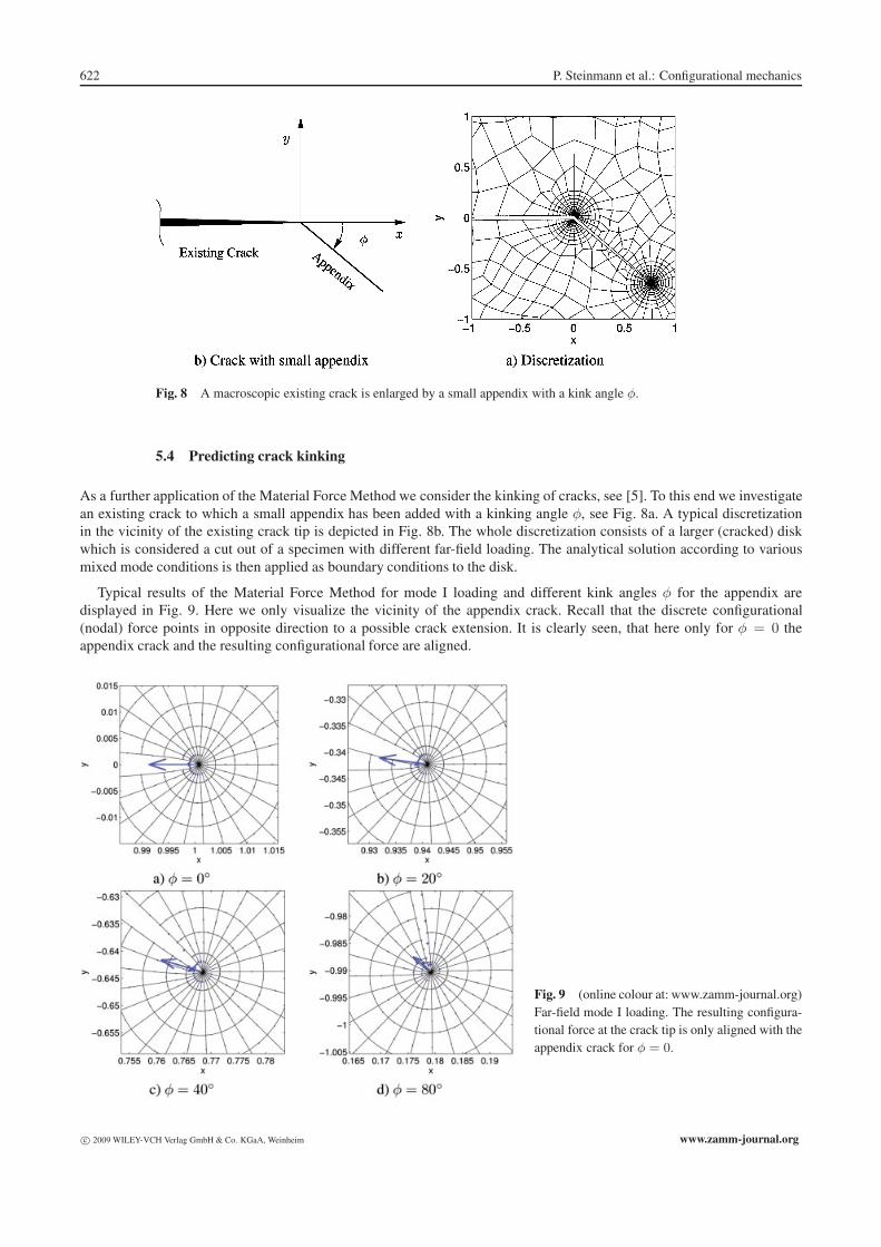
Fig. 8 A macroscopic existing crack is enlarged by a small appendix with a kink angle φ.

5.4 Predicting crack kinking

As a further application of the Material Force Method we consider the kinking of cracks, see [5]. To this end we investigatean existing crack to which a small appendix has been added with a kinking angle φ, see Fig. 8a. A typical discretizationin the vicinity of the existing crack tip is depicted in Fig. 8b. The whole discretization consists of a larger (cracked) diskwhich is considered a cut out of a specimen with different far-field loading. The analytical solution according to variousmixed mode conditions is then applied as boundary conditions to the disk.

Typical results of the Material Force Method for mode I loading and different kink angles φ for the appendix aredisplayed in Fig. 9. Here we only visualize the vicinity of the appendix crack. Recall that the discrete configurational(nodal) force points in opposite direction to a possible crack extension. It is clearly seen, that here only for φ = 0 theappendix crack and the resulting configurational force are aligned.

Fig. 9 (online colour at: www.zamm-journal.org)Far-field mode I loading. The resulting configura-tional force at the crack tip is only aligned with theappendix crack for φ = 0.



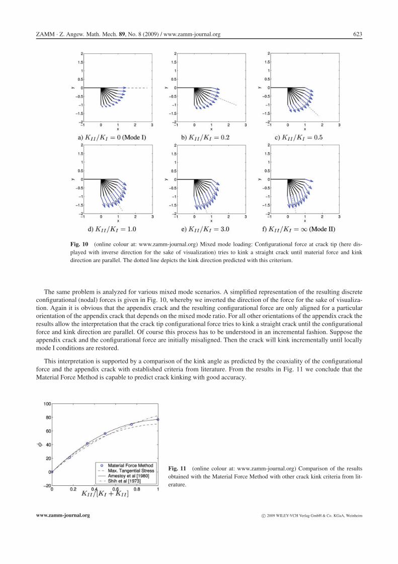
Fig. 10 (online colour at: www.zamm-journal.org) Mixed mode loading: Configurational force at crack tip (here dis-played with inverse direction for the sake of visualization) tries to kink a straight crack until material force and kinkdirection are parallel. The dotted line depicts the kink direction predicted with this criterium.

The same problem is analyzed for various mixed mode scenarios. A simplified representation of the resulting discreteconfigurational (nodal) forces is given in Fig. 10, whereby we inverted the direction of the force for the sake of visualiza-tion. Again it is obvious that the appendix crack and the resulting configurational force are only aligned for a particularorientation of the appendix crack that depends on the mixed mode ratio. For all other orientations of the appendix crack theresults allow the interpretation that the crack tip configurational force tries to kink a straight crack until the configurationalforce and kink direction are parallel. Of course this process has to be understood in an incremental fashion. Suppose theappendix crack and the configurational force are initially misaligned. Then the crack will kink incrementally until locallymode I conditions are restored.

This interpretation is supported by a comparison of the kink angle as predicted by the coaxiality of the configurationalforce and the appendix crack with established criteria from literature. From the results in Fig. 11 we conclude that theMaterial Force Method is capable to predict crack kinking with good accuracy.

Fig. 11 (online colour at: www.zamm-journal.org) Comparison of the resultsobtained with the Material Force Method with other crack kink criteria from lit-erature.



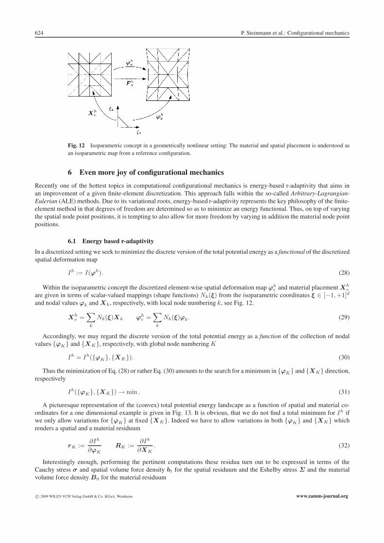
Fig. 12 Isoparametric concept in a geometrically nonlinear setting: The material and spatial placement is understood asan isoparametric map from a reference configuration.

6 Even more joy of configurational mechanics

Recently one of the hottest topics in computational configurational mechanics is energy-based r-adaptivity that aims inan improvement of a given finite-element discretization. This approach falls within the so-called Arbitrary-Lagrangian-Eulerian (ALE) methods. Due to its variational roots, energy-based r-adaptivity represents the key philosophy of the finite-element method in that degrees of freedom are determined so as to minimize an energy functional. Thus, on top of varyingthe spatial node point positions, it is tempting to also allow for more freedom by varying in addition the material node pointpositions.

6.1 Energy based r-adaptivity

In a discretized setting we seek to minimize the discrete version of the total potential energy as a functional of the discretizedspatial deformation map

Ih := I(ϕh). (28)

Within the isoparametric concept the discretized element-wise spatial deformation map ϕhe and material placement Xh

e

are given in terms of scalar-valued mappings (shape functions) Nk(ξ) from the isoparametric coordinates ξ ∈ [−1, +1]d

and nodal values ϕk and Xk, respectively, with local node numbering k, see Fig. 12.

Xhe =

∑k

Nk(ξ)Xk ϕhe =

∑k

Nk(ξ)ϕk. (29)

Accordingly, we may regard the discrete version of the total potential energy as a function of the collection of nodalvalues {ϕK} and {XK}, respectively, with global node numbering K

Ih = Ih({ϕK}, {XK}). (30)

Thus the minimization of Eq. (28) or rather Eq. (30) amounts to the search for a minimum in {ϕK} and {XK} direction,respectively

Ih({ϕK}, {XK}) → min . (31)

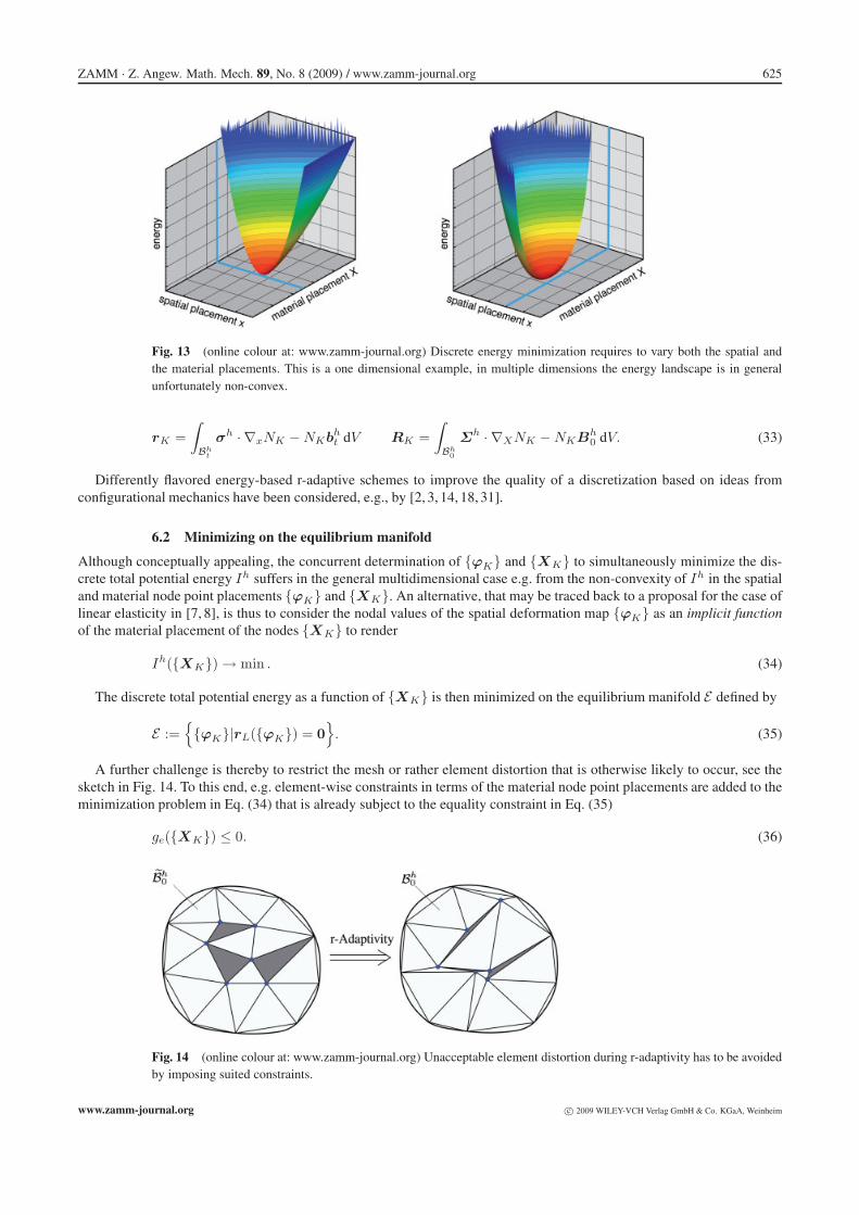
A picturesque representation of the (convex) total potential energy landscape as a function of spatial and material co-ordinates for a one dimensional example is given in Fig. 13. It is obvious, that we do not find a total minimum for Ih ifwe only allow variations for {ϕK} at fixed {XK}. Indeed we have to allow variations in both {ϕK} and {XK} whichrenders a spatial and a material residuum

rK :=∂Ih

∂ϕK

RK :=∂Ih

∂XK. (32)

Interestingly enough, performing the pertinent computations these residua turn out to be expressed in terms of theCauchy stress σ and spatial volume force density bt for the spatial residuum and the Eshelby stress Σ and the materialvolume force density B0 for the material residuum



Fig. 13 (online colour at: www.zamm-journal.org) Discrete energy minimization requires to vary both the spatial andthe material placements. This is a one dimensional example, in multiple dimensions the energy landscape is in generalunfortunately non-convex.

rK =∫Bh

t

σh · ∇xNK − NKbht dV RK =

∫Bh

0

Σh · ∇XNK − NKBh0 dV. (33)

Differently flavored energy-based r-adaptive schemes to improve the quality of a discretization based on ideas fromconfigurational mechanics have been considered, e.g., by [2, 3, 14, 18, 31].

6.2 Minimizing on the equilibrium manifold

Although conceptually appealing, the concurrent determination of {ϕK} and {XK} to simultaneously minimize the dis-crete total potential energy Ih suffers in the general multidimensional case e.g. from the non-convexity of Ih in the spatialand material node point placements {ϕK} and {XK}. An alternative, that may be traced back to a proposal for the case oflinear elasticity in [7, 8], is thus to consider the nodal values of the spatial deformation map {ϕK} as an implicit functionof the material placement of the nodes {XK} to render

Ih({XK}) → min . (34)

The discrete total potential energy as a function of {XK} is then minimized on the equilibrium manifold E defined by

E :={{ϕK}|rL({ϕK}) = 0

}. (35)

A further challenge is thereby to restrict the mesh or rather element distortion that is otherwise likely to occur, see thesketch in Fig. 14. To this end, e.g. element-wise constraints in terms of the material node point placements are added to theminimization problem in Eq. (34) that is already subject to the equality constraint in Eq. (35)

ge({XK}) ≤ 0. (36)

Fig. 14 (online colour at: www.zamm-journal.org) Unacceptable element distortion during r-adaptivity has to be avoidedby imposing suited constraints.



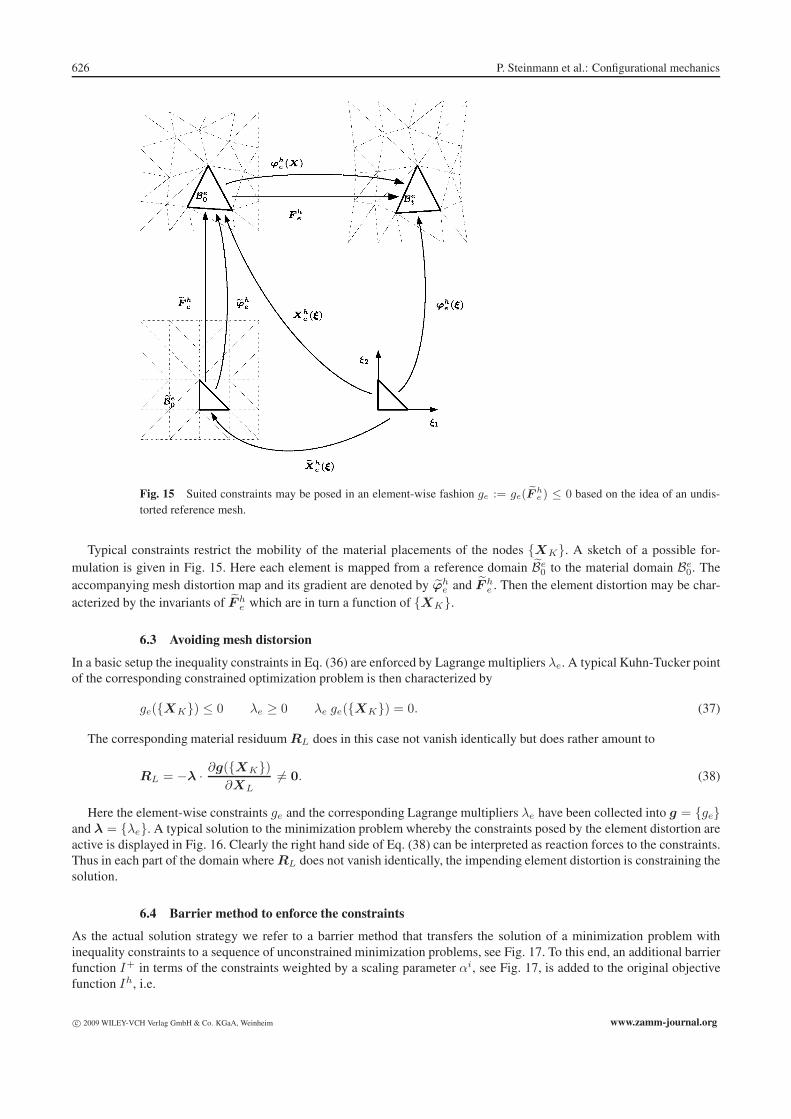
Fig. 15 Suited constraints may be posed in an element-wise fashion ge := ge(Fhe ) ≤ 0 based on the idea of an undis-

torted reference mesh.

Typical constraints restrict the mobility of the material placements of the nodes {XK}. A sketch of a possible for-mulation is given in Fig. 15. Here each element is mapped from a reference domain Be

0 to the material domain Be0. The

accompanying mesh distortion map and its gradient are denoted by ϕhe and F h

e . Then the element distortion may be char-acterized by the invariants of F h

e which are in turn a function of {XK}.

6.3 Avoiding mesh distorsion

In a basic setup the inequality constraints in Eq. (36) are enforced by Lagrange multipliers λe. A typical Kuhn-Tucker pointof the corresponding constrained optimization problem is then characterized by

ge({XK}) ≤ 0 λe ≥ 0 λe ge({XK}) = 0. (37)

The corresponding material residuum RL does in this case not vanish identically but does rather amount to

RL = −λ · ∂g({XK})∂XL

�= 0. (38)

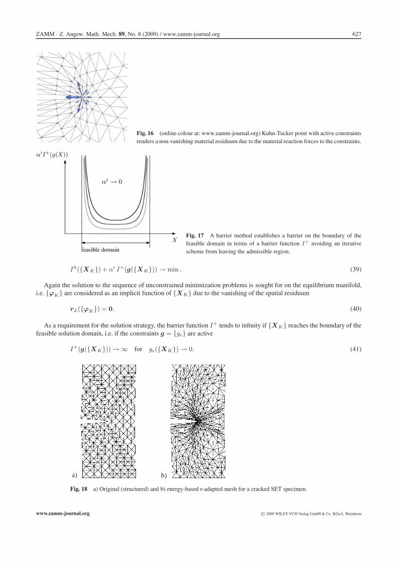
Here the element-wise constraints ge and the corresponding Lagrange multipliers λe have been collected into g = {ge}and λ = {λe}. A typical solution to the minimization problem whereby the constraints posed by the element distortion areactive is displayed in Fig. 16. Clearly the right hand side of Eq. (38) can be interpreted as reaction forces to the constraints.Thus in each part of the domain where RL does not vanish identically, the impending element distortion is constraining thesolution.

6.4 Barrier method to enforce the constraints

As the actual solution strategy we refer to a barrier method that transfers the solution of a minimization problem withinequality constraints to a sequence of unconstrained minimization problems, see Fig. 17. To this end, an additional barrierfunction I+ in terms of the constraints weighted by a scaling parameter αi, see Fig. 17, is added to the original objectivefunction Ih, i.e.



Fig. 16 (online colour at: www.zamm-journal.org) Kuhn-Tucker point with active constraintsrenders a non-vanishing material residuum due to the material reaction forces to the constraints.

Fig. 17 A barrier method establishes a barrier on the boundary of thefeasible domain in terms of a barrier function I+ avoiding an iterativescheme from leaving the admissible region.

Ih({XK}) + αi I+(g({XK})) → min . (39)

Again the solution to the sequence of unconstrained minimization problems is sought for on the equilibrium manifold,i.e. {ϕK} are considered as an implicit function of {XK} due to the vanishing of the spatial residuum

rL({ϕK}) = 0. (40)

As a requirement for the solution strategy, the barrier function I+ tends to infinity if {XK} reaches the boundary of thefeasible solution domain, i.e. if the constraints g = {ge} are active

I+(g({XK})) → ∞ for ge({XK}) → 0. (41)

Fig. 18 a) Original (structured) and b) energy-based r-adapted mesh for a cracked SET specimen.



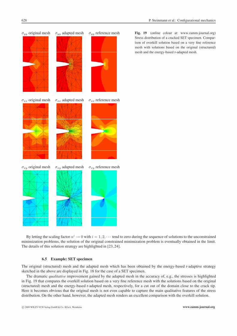
σyy original mesh σyy adapted mesh σyy reference mesh

σxx original mesh σxx adapted mesh σxx reference mesh

σxy original mesh σxy adapted mesh σxy reference mesh

Fig. 19 (online colour at: www.zamm-journal.org)Stress distribution of a cracked SET specimen. Compar-ison of overkill solution based on a very fine referencemesh with solutions based on the original (structured)mesh and the energy-based r-adapted mesh.

By letting the scaling factor αi → 0 with i = 1, 2, · · · tend to zero during the sequence of solutions to the unconstrainedminimization problems, the solution of the original constrained minimization problem is eventually obtained in the limit.The details of this solution strategy are highlighted in [23, 24].

6.5 Example: SET specimen

The original (structured) mesh and the adapted mesh which has been obtained by the energy-based r-adaptive strategysketched in the above are displayed in Fig. 18 for the case of a SET specimen.

The dramatic qualitative improvement gained by the adapted mesh in the accuracy of, e.g., the stresses is highlightedin Fig. 19 that compares the overkill solution based on a very fine reference mesh with the solutions based on the original(structured) mesh and the energy-based r-adapted mesh, respectively, for a cut out of the domain close to the crack tip.Here it becomes obvious that the original mesh is not even capable to capture the main qualitative features of the stressdistribution. On the other hand, however, the adapted mesh renders an excellent comparison with the overkill solution.



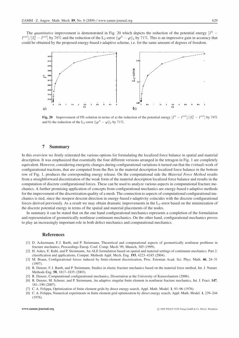
The quantitative improvement is demonstrated in Fig. 20 which depicts the reduction of the potential energy [Ih −Iref ]/[Ih

0 − Iref ] by 78% and the reduction of the L2-error ‖ϕh − ϕ‖2 by 71%. This is an impressive gain in accuracy thatcould be obtained by the proposed energy-based r-adaptive scheme, i.e. for the same amount of degrees of freedom.

Fig. 20 Improvement of FE-solution in terms of a) the reduction of the potential energy [Ih − Iref ]/[Ih0 − Iref ] by 78%

and b) the reduction of the L2-error ‖ϕh − ϕ‖2 by 71%.

7 Summary

In this overview we firstly reiterated the various options for formulating the localized force balance in spatial and materialdescription. It was emphasized that essentially the four different versions arranged in the tetragon in Fig. 1 are completelyequivalent. However, considering energetic changes during configurational variations it turned out that the (virtual) work ofconfigurational tractions, that are computed from the flux in the material description localized force balance in the bottomrow of Fig. 1, produces the corresponding energy release. On the computational side the Material Force Method resultsfrom a straightforward discretization of the weak form of the material description localized force balance and results in thecomputation of discrete configurational forces. These can be used to analyze various aspects in computational fracture me-chanics. A further promising application of concepts from configurational mechanics are energy-based r-adaptive methodsfor the improvement of the discretization quality of a mesh. The connection to aspects of computational configurational me-chanics is tied, since the steepest descent direction in energy-based r-adaptivity coincides with the discrete configurationalforces derived previously. As a result we may obtain dramatic improvements in the L2-error based on the minimization ofthe discrete potential energy in terms of the spatial and material placements of the nodes.

In summary it can be stated that on the one hand configurational mechanics represents a completion of the formulationand representation of geometrically nonlinear continuum mechanics. On the other hand, configurational mechanics provesto play an increasingly important role in both defect mechanics and computational mechanics.

References

[1] D. Ackermann, F. J. Barth, and P. Steinmann, Theoretical and computational aspects of geometrically nonlinear problems infracture mechanics, Proceedings Europ. Conf. Comp. Mech.’99, Munich, 385 (1999).

[2] H. Askes, E. Kuhl, and P. Steinmann, An ALE formulation based on spatial and material settings of continuum mechanics. Part 2:classification and applications, Comput. Methods Appl. Mech. Eng. 193, 4223–4245 (2004).

[3] M. Braun, Configurational forces induced by finite-element discretization, Proc. Estonian Acad. Sci. Phys. Math. 46, 24–31(1997).

[4] R. Denzer, F. J. Barth, and P. Steinmann, Studies in elastic fracture mechanics based on the material force method, Int. J. Numer.Methods Eng. 58, 1817–1835 (2003).

[5] R. Denzer, Computational configurational mechanics, Dissertation at the University of Kaiserslautern (2006).[6] R. Denzer, M. Scherer, and P. Steinmann, An adaptive singular finite element in nonlinear fracture mechanics, Int. J. Fract. 147,

181–190 (2007).[7] C. A. Felippa, Optimization of finite element grids by direct energy search, Appl. Math. Model. 1, 93–96 (1976).[8] C. A. Felippa, Numerical experiments in finite element grid optimization by direct energy search, Appl. Math. Model. 1, 239–244

(1976).



[9] S. Govindjee and P. A. Mihalic, Computational methods for inverse finite elastostatics, Comp. Methods Appl. Mech. Eng. 136,47–57 (1996).

[10] S. Govindjee and P. A. Mihalic, Computational methods for inverse deformations in quasi-incompressible finite elasticity, Int. J.Num. Methods Eng. 43, 821–838 (1998).

[11] M. E. Gurtin, On the nature of configurational forces, Arch. Ration. Mech. Anal. 131, 67–100 (1995).[12] M. E. Gurtin, Configurational forces as basic concepts of continuum physics (Springer, New York, 2000).[13] R. Kienzler and G. Herrmann, Mechanics in material space (Springer, Berlin, 2000).[14] E. Kuhl, H. Askes, and P. Steinmann, An ALE formulation based on spatial and material settings of continuum mechanics. Part 1:

generic hyperelastic formulation, Comput. Methods Appl. Mech. Eng. 193, 4207–4222 (2004).[15] G. A. Maugin, Material inhomogeneities in elasticity (Chapman & Hall, London, 1993).[16] G. A. Maugin, Material forces: concepts and applications, Appl. Mech. Rev. 48, 213–245 (1995).[17] C. Miehe and E. Gurses, A robust algorithm for configurational-force-driven brittle crack propagation with R-adaptive mesh

alignment, Int. J. Num. Methods Eng. 72, 127–155 (2007).[18] J. Mosler and M. Ortiz, On the numerical implementation of varational arbitrary Lagrangian-Eulerian (VALE) formulations, Int.

J. Numer. Methods Eng. 67, 1272–1289 (2006).[19] R. Mueller and G. A. Maugin, On material forces and finite element discretizations, Comput. Mech. 29, 52–60 (2002).[20] R. Mueller, S. Kolling, and D. Gross, On configurational forces in the context of the finite element method, Int. J. Numer. Methods

Eng. 53, 1557–1574 (2002).[21] R. Mueller, D. Gross, and G. A. Maugin, Use of material forces in adaptive finite element methods, Comput. Mech. 33, 421–434

(2004).[22] A. Rajagopal, R. Gangadharan, and S. M. Sivakumar, On material forces and finite element discretizations, Int. J. Comput. Meth-

ods Eng. Sci. Mech. 7, 241–262 (2006).[23] M. Scherer, R. Denzer, and P. Steinmann, Energy-based r-adaptivity: a solution strategy and applications to fracture mechanics,

Int. J. Fract. 147, 117–132 (2007).[24] M. Scherer, R. Denzer, and P. Steinmann, On a solution strategy for energy-based mesh optimization in finite hyperelastostatics,

Comp. Methods Appl. Mech. Eng. 197, 609–622 (2008).[25] P. Steinmann, Application of material forces to hyperelastostatic fracture mechanics. Part I: Continuum mechanical setting, Int. J.

Solids Struct. 37, 7371–7391 (2000.)[26] P. Steinmann, D. Ackermann, and F. J. Barth, Application of material forces to hyperelastostatic fracture mechanics. Part II:

computational setting, Int. J. Solids Struct. 38, 5509–5526 (2001).[27] P. Steinmann, On spatial and material settings of hyperelastodynamics, Acta Mechanica 156, 193–218 (2002).[28] P. Steinmann, On spatial and material settings of thermo-hyperelastodynamics, J. Elasticity 66, 109–157 (2002).[29] P. Steinmann, On spatial and material settings of hyperelastostatic crystal defects, J. Mech. Phys. Solids 50, 1743–1766 (2002).[30] P. Steinmann, On boundary potential energies in deformational and configurational mechanics, J. Mech. Phys. Solids 56, 772–800

(2008).[31] P. Thoutireddy and M. Ortiz, A variational r-adaption and shape-optimization method for finite-deformation elasticity, Int. J.

Numer. Methods Eng. 61, 1–21 (2004).[32] D. K. Vu and P. Steinmann, Nonlinear electro- and magneto-elastostatics: material and spatial settings, Int. J. Solids Struct. 44,

7891–7905 (2007).


Documents

Secret and joy of configurational mechanics: From foundations in continuum mechanics to applications in computational mechanics