Embed Size (px)
Citation preview

Deliverable on Railway electromagnetic environment analysis Date: 24/07/2013
Distribution: All partners Manager: IFSTTAR
SECRET SECurity of Railways against
Electromagnetic aTtacks Grant Agreement number: 285136 Funding Scheme: Collaborative project Start date of the contract: 01/08/2012 Project website address: http://www.secret-project .eu
Deliverable D 3.1 "Synthesis model" for experimental simulation of normal and attack conditions: methodology and results
Submission date: 24 th July 2013

SECRET Project Grant Agreement number: 285136
SEC-D3.1-C-07 2013-"Synthesis model" for experimental simulation of normal and attack conditions-IFSTTAR 24/07/2013 2/42
Document details:
Title "Synthesis model" for experimental simulation of no rmal and attack conditions: methodology and results
Workpackage WP3
Date 28/06/2013
Author(s) M. Heddebaut, J.P. Ghys, S. Ambellouis, D. Sodoyer, V. Deniau, S. Mili V. Beauvois, H. Philippe
Responsible Partner IFSTTAR
Document Code SEC-D3.1-C-07 2013-Synthesis model for experimental simulation of normal and attack conditions-IFSTTAR
Version C
Status Final
Dissemination level:
Project co-funded by the European Commission within the Seventh Framework Programme
PU Public X
PP Restricted to other programme participants (including the Commission Services)
RE Restricted to a group specified by the consortium (including the Commission) Services)
CO Confidential, only for members of the consortium (including the Commission Services)
Document history:
Revision Date Authors Description
Initial version 28/06/2013 M. Heddebaut, J.P. Ghys, S. Ambellouis, D. Sodoyer, V. Deniau, S. Mili, V. Beauvois, H. Philippe
Draft v1.0
Minor modifications
08/07/210 / v1.1
Minor modifications after reviewing
11/07/210 / v1.2

SECRET Project Grant Agreement number: 285136
SEC-D3.1-C-07 2013-"Synthesis model" for experimental simulation of normal and attack conditions-IFSTTAR 24/07/2013 3/42
Table of content
1. Executive summary ___________________________________________________ 6
2. Introduction __________________________________________________________ 6
2.1. Purpose of the document ________________________________________________ 6
2.2. Definitions and acronyms ________________________________________________ 6
3. Considered railway critical systems ____________________________________ 8
3.1. Ground to train communication based on GSM-R __________________________ 9
3.2. Railway station operation based on TETRA _______________________________ 9
3.3. Train location and services based on GNSS/GPS _________________________ 10
3.4. Spot communication using EUROBALISE ________________________________ 11
3.5. Conclusion ____________________________________________________________ 12
4. Railway critical environments to be considered ________________________ 12
4.1. Lines __________________________________________________________________ 12
4.2. Stations _______________________________________________________________ 12
5. European selected railway sites and configurations ____________________ 14
5.1. LGV Est _______________________________________________________________ 14
5.2. Paris Gare de l’Est _____________________________________________________ 14
5.3. Liège Guillemins _______________________________________________________ 15
6. Normal environment measurement setup ______________________________ 16
7. Results of in situ measurement campaigns ____________________________ 17
7.1. Measurements along the LGV Est from France to Germa ny ________________ 17
7.2. Measurements in Paris Gare de l’Est ____________________________________ 20
7.2.1. Results obtained along the platform (Gare de l’Est - loc. A) ______________________ 22 7.2.2. Results in front of the control-command centre (Gare de l’Est - loc. B) ____________ 24 7.2.3. Junction between the railway and the subway stations (Gare de l’Est - loc. C) ______ 26
7.3. Measurements in Liège Guillemins ______________________________________ 27
8. Inputs for the definition of normal EM conditions _______________________ 30
8.1. TETRA 410-430 MHz ____________________________________________________ 30
8.2. GSM-R ________________________________________________________________ 30
8.2.1. Downlink frequency band 921-925 MHz _______________________________________ 30 8.2.2. Uplink frequency band 876-880 MHz __________________________________________ 30
8.3. GNSS - Civilian GPS ____________________________________________________ 32
8.4. EUROBALISE __________________________________________________________ 32
9. Anomaly detection techniques ________________________________________ 32
9.1. Introduction ___________________________________________________________ 32
9.2. Generalities ____________________________________________________________ 33
9.3. Description of the most common techniques _____________________________ 33
9.3.1. Discriminative methods ______________________________________________________ 33

SECRET Project Grant Agreement number: 285136
SEC-D3.1-C-07 2013-"Synthesis model" for experimental simulation of normal and attack conditions-IFSTTAR 24/07/2013 4/42
9.3.2. Generative methods ________________________________________________________ 34
9.4. Towards EM anomaly detection _________________________________________ 35
9.5. Bibliography of section 9 _______________________________________________ 35
10. Preliminary results using the experimental collected data _____________ 36
10.1. Analysis and model of the EM environment _____________________________ 36
10.1.1. Introduction and context ____________________________________________________ 36 10.1.2. Analysis and Characterization of the EM environment in normal conditions _______ 36 10.1.3. EM model : Intrinsic variations and variations in function of time ________________ 40 10.1.4. EM Spectrum model: Variations in function the location observation. ____________ 41
11. Conclusion ________________________________________________________ 41
12. Acknowledgements ________________________________________________ 41

SECRET Project Grant Agreement number: 285136
SEC-D3.1-C-07 2013-"Synthesis model" for experimental simulation of normal and attack conditions-IFSTTAR 24/07/2013 5/42
List of figures
Figure 1: ERTMS/ETCS targets for EM threats ...................................................................................... 8 Figure 2: Eurobalise/BTM transmissions principle ................................................................................ 11 Table 1: Railway systems and associated electromagnetic parameters .............................................. 12 Figure 3: LGV Est line as seen from a measurement site ..................................................................... 14 Figure 4: Tracks and platforms of the Paris Gare de l’Est .................................................................... 15 Figure 5: Tracks and platforms of the Liège Gare des Guillemins ........................................................ 15 Figure 6a: Electric field measurement using the conical dipole (Paris, gare de l’Est) .......................... 16 Figure 6b: Magnetic field measurement using the active loop (Liège, Guillemins gare) ...................... 16 Figure 7a: Laboratory van and wideband conical dipole installed on top the van along LGV Est ........ 16 Figure 7b: Measuring equipment inside the laboratory van .................................................................. 16 Figure 8: 875-975 MHz GSM-R downlink LGV Est record .................................................................... 17 Figure 9: 918-928 MHz GSM-R downlink LGV Est ............................................................................... 18 Figure 10: 922 MHz BTS centered record – span = 120 kHz ............................................................... 18 Figure 11: 873-883 MHz GSM-R uplink LGV Est record ...................................................................... 19 Figure 12: GPS-L1 typical LGV Est record ............................................................................................ 19 Figure 13: Eurobalise 27 MHz band typical record ............................................................................... 20 Figure 14: Measurement locations on a platform (A), in front of the station control room (loc. A & B) . 21 Figure 15: Measurement at the junction between railway and subway stations (loc. C). ..................... 21 Figure 16: GSM-R downlink frequencies - span = 100 MHz (Gare de l’Est - loc. A). ........................... 22 Figure 17: GSM-R downlink frequencies - span = 10 MHz (Gare de l’Est - loc. A). ............................. 22 Figure 18: GSM-R uplink frequencies - span = 10 MHz (Gare de l’Est - loc. A). .................................. 23 Figure 19: GPS L1 civilian frequency - span = 2 MHz (Gare de l’Est - loc. A). ..................................... 23 Figure 20: Measurements at TETRA frequencies - span = 40 MHz (Gare de l’Est - loc. B). ................ 24 Figure 21: Measurements at TETRA frequencies - span = 20 kHz (Gare de l’Est - loc. B). ................. 24 Figure 22: GSM-R downlink frequencies - span = 100 MHz (Gare de l’Est - loc. B). ........................... 25 Figure 23: GSM-R downlink frequency band - span = 10 MHz (Gare de l’Est - loc. B). ....................... 25 Figure 24: GSM-R uplink frequencies - span = 10 MHz (Gare de l’Est - loc. B). .................................. 26 Figure 25: TETRA frequencies - span = 40 MHz (Gare de l’Est - loc. C). ............................................ 26 Figure 26: GSM-R downlink frequencies - span = 10 MHz (Gare de l’Est - loc. C). ............................. 27 Figure 27: GSM-R downlink frequencies - span = 100 MHz (Guillemins)............................................. 27 Figure 28: GSM-R downlink frequencies - span = 10 MHz (Guillemins) ............................................... 28 Figure 29: GSM-R uplink frequencies - span = 10 MHz (Guillemins) ................................................... 28 Figure 30: Eurobalise train interrogator signals - span = 10 MHz (Guillemins) .................................... 29 Figure 31: GPS L1 civilian frequency - span = 2 MHz (Guillemins). ..................................................... 29 Figure 32: Illustration of normal and anomalous behaviour in a 2D space. N1 and N2 are “normal” subspaces. o1, o2 and o3 are “anomalous” points and subspace ........................................................ 33 Figure 33: Illustration of multi-class and one-class anomaly detection ................................................. 34 Figure 34: Spectra of GSM-R downlink frequencies - Gare de l'Est, in station .................................... 37 Figure 35: Spectra of GSM-R downlink frequencies - Gare de l'Est, along a platform. ........................ 37 Figure 36: Spectra of GSM-R downlink frequencies – Liège Guillemins, at the platform level. ............ 38 Figure 37: Spectra of GSM-R downlink frequencies – Liège Guillemins, at level -1............................. 38 Figure 38: Spectra of GSM-R downlink frequencies – LGV Est, location 1. ......................................... 39 Figure 39: Spectra of GSM-R downlink frequencies – LGV Est, location 2. ......................................... 39 Figure 40: A sequence of 500 consecutive samples of the spectrum at the frequency f= 922 MHz. LGV Est, location 2. ....................................................................................................................................... 41

SECRET Project Grant Agreement number: 285136
SEC-D3.1-C-07 2013-"Synthesis model" for experimental simulation of normal and attack conditions-IFSTTAR 24/07/2013 6/42
1. Executive summary
In deliverable D3.1, “normal” EM conditions are preliminary measured and defined in order to constitute reference conditions for the development involved in WP3. In this deliverable, the methodology and the experimental conditions employed to collect reference noise conditions are described. Experimental results performed in European critical railway sites are reported. Theoretical techniques to determine a normal electromagnetic environment are presented.
2. Introduction
2.1. Purpose of the document
The ERTMS/ETCS critical systems and associated railway equipments are deduced from the previous Secret EM threats Tests strategy work (WP1).
The purpose of this document is to consider the railway critical systems that are in the scope of this Secret WP3 activity, then to define the corresponding frequency bands of interest to be investigated. In a second step, we consider some railway critical environments to be evaluated and select representative sites where to measure significant electromagnetic environments.
Suitable measuring equipment is then selected and described.
In situ measurements where performed during several campaigns; some significant results are reported in this deliverable.
Theoretical techniques that can be used to determine reference normal conditions using these results are presented.
2.2. Definitions and acronyms
Meaning
ASK Amplitude Shift Keying
BTM Balise Transmission Module
BTS Base Transceiver Station
CCS Control Command and Signalling subsystems
CENELEC European Committee for Electro technical Standardization
DMO Direct Mode Operation
EIRENE European Integrated Railway Radio Enhanced Network
EMC ElectroMagnetic Compatibility
ERTMS European Railways Traffic Management System
ETCS European Train Control System
ETSI European Telecommunications Standards Institute
EU European Union
GNSS Global Navigation Satellite System
GMSK Gaussian Minimum Shift Keying
GPS Global Positioning System
GSM Global System for Mobile communications
GSM-R Global System for Mobile communications - Railways
HSL High Speed Line
ICE Inter City Express

SECRET Project Grant Agreement number: 285136
SEC-D3.1-C-07 2013-"Synthesis model" for experimental simulation of normal and attack conditions-IFSTTAR 24/07/2013 7/42
Meaning
JRU Juridical Recording Unit
KVB Contrôle de vitesse par balise
LEU Lineside Equipment Unit
LGV Ligne à Grande Vitesse (HSL)
LOS Line of Sight
LTM Loop Transmission Module
MCS Master Control Station
MMI Man-Machine Interface
PVT Position, Velocity and Time
RBC Radio Block Center
STM Specific Transmission Module
TETRA Terrestrial Trunked Radio
TGV Train à Grande Vitesse
TIU Train Interface Unit
TMO Trunked Mode Operation
TSI Technical Specification for Interoperability

SECRET Project Grant Agreement number: 285136
SEC-D3.1-C-07 2013-"Synthesis model" for experimental simulation of normal and attack conditions-IFSTTAR 24/07/2013 8/42
3. Considered railway critical systems
The following elements are extracted from the Secret deliverable “ERTMS L1 EM threats Test strategy document”, Feb. 2013. The ERTMS/ETCS reference architecture is provided in CCS TSI documentation, in particular in subset-026. The TSI documentation is accessible at http://www.era.europa.eu/Core-Activities/ERTMS/Pages/home.aspx. The following figure 1 (see subset-026) indicates the ERTMS reference architecture and the ALSTOM view on the potential radio interface targets for EM threats & malicious attacks.
Figure 1: ERTMS/ETCS targets for EM threats Source Secret deliverable ERTMS L1 EM threats Test strategy document, Feb. 2013)
As represented in this Figure 1, “Secret” partners have already identified major ERTMS/ETCS targets for electromagnetic threats. They are mainly related to the use of the GSM-R for train to ground communication, the use of GNSS/GPS satellite navigation received signals for the train odometry system and the Eurobalise/Balise Transmission Module or KVB for spot communication. The trackside fixed transmission networks (e.g. backbone, track circuits, axle counters…) could also be considered later on for further studies.
This section will briefly present the different radio communication and navigation systems that will be considered in the study; the frequency bands to be surveyed will be indicated.
We will add to this existing list the TETRA Terrestrial Trunked Radio system which was also considered many years ago for ground to train radio communication. TETRA is currently used by

SECRET Project Grant Agreement number: 285136
SEC-D3.1-C-07 2013-"Synthesis model" for experimental simulation of normal and attack conditions-IFSTTAR 24/07/2013 9/42
some railway operators for railway and depots communication and also for railway security applications.
3.1. Ground to train communication based on GSM-R
GSM-R is a standard communication platform for railway system. It is a strategic communication system focused on interoperability between European railway infrastructures. It is now deployed over the world. By the end of 2016, 56 countries in five continents should have operational GSM-R network. Europe is leading GSM-R implementation through mainly 11 countries (Austria, Belgium, Czech Republic, France, Germany, Italy, the Netherlands, Norway, Spain, Sweden and Switzerland). In 2011, GSM-R deployment provides coverage about 30% of European railway network with 68.000 km in operation; 156.000 km are planned to be covered (70% of European railway network).
The main objectives of GSM-R are to replace analogical radio communication (RST Radio Sol Train, ground to train radio telecommunications network) and to provide data transmission solution for ERTMS/ETCS (European Rail Traffic Management System / European Train Control System) level 2 and level 3.
GSM-R is an evolution of public GSM dedicated to railway application. Therefore GSM-R has similar characteristics than public GSM system. GSM-R functionality is built on standards and recommendations supported by mainly two organizations, ETSI (European Telecommunications Standards Institute) and UIC (Union Internationale des Chemins de fer, International Union of Railways). ETSI technical committee RT (Railway Telecommunications) is responsible for those aspects of Global System for Mobile communications standardization which are specific to Railway (GSM-R) and Private Mobile Radio (PMR) operations. UIC specifies through its project EIRENE (European Integrated Railway Radio Enhanced Network) a digital radio standard for the European railways. It forms part of the specification for technical interoperability.
GSM-R performances are guaranteed for high-speed conditions (up to 500 km/h). A common European frequency band is allocated to GSM-R below the frequencies of the public GSM standard. The allocated frequency bands are:
For the uplink: 876 MHz - 880 MHz
For the downlink: 921 MHz - 925 MHz
Therefore, these two frequency bands will be considered to evaluate what are the normal operating conditions in the different selected Secret Project railway environments. Moreover, to take into account potential extensions of these frequency bands, wider frequency ranges will be considered during the definition of normal electromagnetic environments.
The GSM-R network is designed to provide a minimum level of received power > -95 dBm, this is a mandatory requirement coming from the EIRENE specifications. This represents a limited level of power with the potential of being jammed.
3.2. Railway station operation based on TETRA
Terrestrial Trunked RAdio (TETRA) is a professional mobile radio and two-way transceiver specification. TETRA was specifically designed for use by government agencies, emergency services (police forces, fire departments, ambulance) for public safety networks, rail transportation staff for train radios, transport services and the military.
The TETRA standard has been specifically developed to meet the needs of a variety of traditional PMR user organisations. This means it has a scalable architecture allowing economic network deployments ranging from single site local area coverage to multiple site wide area national coverage. Some unique PMR services of TETRA are:
• Wide area fast call set-up "all informed net" group calls • High level voice encryption to meet the security needs of public safety organizations • An Emergency Call facility that gets through even if the system is busy • Full duplex voice for PABX and PSTN telephony communications
In Trunked Mode Operation (TMO), TETRA mobile radios are used in combination with network infrastructure. Direct Mode Operation (DMO) maintains TETRA radio communication between mobile radios without using a TETRA network infrastructure.

SECRET Project Grant Agreement number: 285136
SEC-D3.1-C-07 2013-"Synthesis model" for experimental simulation of normal and attack conditions-IFSTTAR 24/07/2013 10/42
A common European frequency band is not allocated to TETRA. In France, the 410 MHz to 430 MHz & 450 to 470 MHz bands are allocated in the Paris area. Therefore, these frequency bands and especially the first one will be considered in WP3.
At SNCF, TETRA radio services includes 6 TMO networks in Paris railway stations: Gare de Lyon, Paris Nord, Saint Lazare… involving 1,800 users. In French regions, 4 TMO exist in major cities (Lyon, Strasbourg, Bordeaux, Marseille) involving 600 users. DMO mode is also used for local operational needs. Specific developments (TMO/DMO) have been performed concerning:
• Shunting • Data Services to SNCF activities • Track maintenance operations • Network interfacing • Remote command for train “ready for departure” • Remote command for cross gate
In the future SNCF radio networks will be 100% TETRA. Some other European railway operators are also considering TETRA.
There also exists a specific TETRA network named Iris 2 dedicated to railway security. It was deployed in 1994 in Ile de France and is in service since 1996. Its major characteristics are high communication availability, secured communications and permanent user location. It provides extended radio coverage at 50 km around Paris and a high radio coverage quality (tunnels, stations ...). The main users are for the railway operator security staff and the police.
TETRA networks could be a target of EM attacks for increasing damages of terrorist attacks.
3.3. Train location and services based on GNSS/GPS
The possible applications of Global Navigation satellite System (GNSS) in the rail sector are numerous. Global Positioning System (GPS) is probably the best known satellite navigation system. A distinction shall be made between the non safety-critical applications (fleet supervision, passenger information…) and the safety-critical applications (train control, train integrity, train awakening…). Concerning the non-safety critical applications, GNSS is already used today, fulfilling various functions. Concerning the safety-critical functions, GNSS has the potential to be used for ERTMS/ETCS by enhancing odometry, increasing their reliability in future trains. However, this capability is still to be verified.
A Global Navigation Satellite System is a space-based radio-positioning and time transfer system. GNSS provides accurate position, velocity, and time (PVT) information to an unlimited number of suitably equipped ground, sea, air and space users. Passive PVT fixes are available world-wide in all-weathers in a world-wide common grid system. GNSS comprises three major system segments, Space, Control, and User.
A GNSS Space Segment consists of a constellation of satellites in semi-synchronous (approximately 12-hour) orbits. The satellites are arranged in a number of orbital planes with several satellites in each plane.
The Control Segment primarily consists of a Master Control Station (MCS) plus monitor stations and ground antennas at various locations around the world. The MCS is the central processing facility for the Control Segment and is responsible for monitoring and managing the satellite constellation. The MCS functions include control of satellite station-keeping maneuvers, reconfiguration of redundant satellite equipment, regularly updating the navigation messages transmitted by the satellites, and various other satellite health, monitoring and maintenance activities. The monitor stations passively track all satellites in view, collecting ranging data from each satellite. This information is transmitted to the MCS where the satellite ephemeris and clock parameters are estimated and predicted. The MCS uses the ground antennas to periodically upload the ephemeris and clock data to each satellite for retransmission in the navigation message.
The User Segment consists of receivers specifically designed to receive, decode, and process the GNSS satellite signals. Receivers can be stand-alone, integrated with or embedded into other systems. GNSS receivers can vary significantly in design and function, depending on their application for navigation, accurate positioning, time transfer, surveying and attitude reference.
The primary benefit of GNSS for railway is that GNSS has the potential to replace many existing ground and train based navigation systems or obviate the need to procure new systems, thereby reducing the cost of maintaining or acquiring these systems. The primary concerns stem from the

SECRET Project Grant Agreement number: 285136
SEC-D3.1-C-07 2013-"Synthesis model" for experimental simulation of normal and attack conditions-IFSTTAR 24/07/2013 11/42
safety-of-life issue and the fact that GNSS signal failures can affect large areas and consequently large numbers of trains simultaneously.
The GPS satellites transmit ranging signals on two frequency bands: Link 1 (L1) at 1575.42 MHz and Link 2 (L2) at 1227.6 MHz. L1 is used for civilian applications, L2 for military applications. The satellite signals are transmitted using spread-spectrum techniques, employing two different ranging codes as spreading functions. In the frequency allocation filing, the L1 power is listed as 25 Watts. The antenna gain is listed at 13 dBi. Thus, based on the frequency allocation filing, the effective isotropic power would be about 500 Watts (27 dBW). The free space path loss from a considered satellite altitude of 21000 km is about 182 dB. Therefore the received power at ground is -125 dBm, a very low level.
In WP3, we will consider the L1 civilian frequency band. We make the assumption that other radiofrequency signals in the same frequency band, providing a received power close to this -125dBm value, can act as potential jammers
3.4. Spot communication using EUROBALISE
The Eurobalise/Balise Transmission Module (BTM) communication is an essential part of ERTMS level 1. The Eurobalises are used for spot transmission from track to train. The Eurobalises must be able to transmit variable information but does not know the train to which it sends information. A Eurobalise is a device that is interrogated and tele-powered by means of an inductively coupled telepowering signal. The response of the Eurobalise is also an inductively coupled uplink signal.
Source and sink of the telepowering signal and the uplink signal respectively is the vehicle mounted Antenna Unit. The following figure 2 represents this description:
Up-link signal
(A1)
Tele-powering signal
(A4)
C interface
Figure 2: Eurobalise/BTM transmissions principle (Source Secret deliverable ERTMS L1 EM threats Test strategy document Feb.2013)
The origin of the data carried by the uplink signal is recorded in a non-volatile memory in the Eurobalise, or received through a serial data-link referenced as Interface 'C' to the Lineside Equipment Unit (LEU). The radio interface between Eurobalise and train antenna with BTM subsystem is called Interface 'A’. The communication path is limited in length (< 1 m).
Downlink radio transmission
The magnetic field is produced by the vehicle mounted Antenna Unit/BTM at a frequency of 27.095 MHz with a tolerance of ± 5 kHz. The signal is a continuous wave (CW). The carrier noise shall be < -110 dBc/Hz at frequency offsets ≥ 10 kHz.
Alternatively, some existing systems are still using KVB balises operating in the same frequency range but also transmitting a clock frequency by ASK modulating the telepowering signal at a frequency of 10 kHz.
Uplink radio transmission

SECRET Project Grant Agreement number: 285136
SEC-D3.1-C-07 2013-"Synthesis model" for experimental simulation of normal and attack conditions-IFSTTAR 24/07/2013 12/42
The magnetic field produces two frequencies that are used for frequency shift keying (FSK) of the Uplink data. The two frequencies are nominally:
o 3.951 MHz for a logical 0 (fL)
o 4.516 MHz for a logical 1 (fH)
Thus, one ‘0’-bit corresponds to approximately 7 periods of 3.951 MHz and one ‘1’-bit corresponds to approximately 8 periods of 4.516 MHz.
In a shift between the two frequencies the carrier shall have a continuous phase, i.e. continuous phase frequency shift keying modulation (CPFSK) shall apply.
o The centre frequency shall be (fH+fL)/2 = 4.234 MHz ± 175 kHz.
o The frequency deviation shall be (fH-fL)/2 = 282.24 kHz ± 7 %.
3.5. Conclusion
The following table 1 summarizes these different railway communication systems of interest in column 1 and the corresponding frequency bands to be investigated in column 2. The last column indicates the type of electric or magnetic field that has to be measured, as well as its orientation.
Railway communication
system Allocated/Used railway frequency band Measurement type
TETRA 410-430 MHz E field,
vertical component
GSM-R 921-925 MHz
(downlink)
E field,
vertical component
GSM-R 876-880 MHz
(uplink)
E field,
vertical component
GNSS
Civilian GPS
L1: 1575.42 MHz
Bandwidth: C/A 2.046 MHz
E field,
vertical component
EUROBALISE 27.095 MHz H field,
Vertical component
Table 1: Railway systems and associated electromagnetic parameters
4. Railway critical environments to be considered
To evaluate normal electromagnetic conditions, it was decided to perform electromagnetic environment measurements in different railway critical environments.
4.1. Lines
To get a general view of a normal railway electromagnetic environment, it was decided to perform electromagnetic environment measurements along a representative railway line where low or medium power jammers could be positioned discreetly, in particular with the objective to jam the ground to train communication based on GSM-R or, a satellite positioning system.
4.2. Stations
It was also decided to measure the electromagnetic environment conditions in railway stations that are

SECRET Project Grant Agreement number: 285136
SEC-D3.1-C-07 2013-"Synthesis model" for experimental simulation of normal and attack conditions-IFSTTAR 24/07/2013 13/42
strategic places where electromagnetic attacks could occur.

SECRET Project Grant Agreement number: 285136
SEC-D3.1-C-07 2013-"Synthesis model" for experimental simulation of normal and attack conditions-IFSTTAR 24/07/2013 14/42
5. European selected railway sites and configuratio ns
5.1. LGV Est
The LGV Est européenne is an extension to the French high-speed rail network. Figure 3 shows a view of this line, as seen from one particular measurement location.
Figure 3: LGV Est line as seen from a measurement site
The line provides fast services between Paris and the principal cities of eastern France and Luxembourg, as well as to several cities in Germany and Switzerland. It also enables fast connections between eastern France and other French regions already served by TGV, to the southeast, the west and southwest, and to the north, with extensions towards Belgium. The first 300 km section of this new route entered service on 10 June 2007. Constructed for speeds up to 350 km/h (220 mph), for commercial service, it is initially operating at a maximum speed of 320 km/h. It is the first line in France to travel at this speed in commercial service, the first to use ERTMS and the first line also served by German ICE trains.
5.2. Paris Gare de l’Est
Two railway stations were selected to be representative for the study: the Paris Gare de l’Est railway station and the Liege Gare des Guillemins railway station.
Gare de l'Est, "East station" is one of the six large SNCF railway stations in Paris. The Gare de l'Est was opened in 1849 by the Compagnie du Chemin de Fer de Paris à Strasbourg. The Gare de l'Est is the terminus of a strategic railway network extending towards the eastern part of France. SNCF started High Speed Train “LGV Est Européenne services” from the Gare de l'Est on 10 June 2007, with TGV and ICE services to north-eastern France, Luxembourg, southern Germany and Switzerland. Trains are initially running at 320 km/h, with the potential to run at 350 km/h. Figure 4 presents a view of the Paris Gare de l’Est environment as seen from a measurement location.

SECRET Project Grant Agreement number: 285136
SEC-D3.1-C-07 2013-"Synthesis model" for experimental simulation of normal and attack conditions-IFSTTAR 24/07/2013 15/42
Figure 4: Tracks and platforms of the Paris Gare de l’Est
5.3. Liège Guillemins
Liège-Guillemins railway station is the main station of the city of Liège, the third largest city in Belgium. It is one of the most important hubs in the country and is one of the three Belgian stations on the high-speed rail network. The station is used by 36,000 people every day which makes it the tenth busiest station in Belgium. The new station by the architect Santiago Calatrava was officially opened on September 18, 2009. It has 9 tracks and 5 platforms (three of 450 m and two of 350 m). All the tracks around the station have been modernized to allow high speed arrival and departure. The new station is made of steel, glass and white concrete. It includes a monumental arch, 160 m long and 32 m high. Liège-Guillemins station is served by InterCity- and InterRegio trains, connecting Liège with all major Belgian cities, as well as several international destinations such as Aachen, Lille, and Maastricht. In addition to the national traffic, Liège-Guillemins station welcomes Thalys and ICE trains, connecting Liège to Brussels, Paris, Aachen, Cologne, and Frankfurt. Two new dedicated high-speed tracks were built: HSL 2 (Brussels-Liège) and HSL 3 (Liège-German border). There are also plans for Eurostar and ICE to link Liège to London directly. Figure 5 presents a view of the Gare des Guillemins environment.
Figure 5: Tracks and platforms of the Liège Gare des Guillemins

SECRET Project Grant Agreement number: 285136
SEC-D3.1-C-07 2013-"Synthesis model" for experimental simulation of normal and attack conditions-IFSTTAR 24/07/2013 16/42
6. Normal environment measurement setup
For the electromagnetic environment measurements, we use an Agilent MXA N9020A signal analyzer covering the frequency band 20 Hz to 8.4 GHz. A computer is integrated into the analyzer so that sequences of measurement can be programmed and the corresponding results stored. A backup hard drive disk was also used. Extensive spectrum and I/Q measurements in the frequency ranges indicated in table 1 were performed and stored. For the electric field measurements, we used an N3200 wide band precision conical dipole antenna coming from Austrian Research Centers. This antenna was used for the TETRA, GSM-R and GPS frequency bands. For the magnetic field measurements, an EMCO model 6507 active loop covering 1 kHz to 30 MHz was selected. This antenna was used to perform the measurements in the Eurobalise telepowering frequency band.
The following figures 6a and 6b show this measuring equipment installed in railway stations with its associated electric and magnetic measuring antennas.
Figure 6a: Electric field measurement using the conical dipole (Paris, gare de l’Est)
Figure 6b: Magnetic field measurement using the active loop (Liège, Guillemins gare)
The following figures 7a and 7b show this equipment and the conical dipole measuring antenna installed in a laboratory van, along the railway line.
Figure 7a: Laboratory van and wideband conical dipole installed on top the van along LGV Est
Figure 7b: Measuring equipment inside the laboratory van
In the following sections, we present a selection of measurement results recorded at the different frequency bands considered for this study (see table 1). To get an accurate representation of the normal electromagnetic conditions, different frequency spans or measured bandwidths were successively selected on the signal analyzer. These spans are wider than the railway allocated frequency band. For example, we used spans of 100 MHz and 10 MHz to analyze the 4 MHz wide

SECRET Project Grant Agreement number: 285136
SEC-D3.1-C-07 2013-"Synthesis model" for experimental simulation of normal and attack conditions-IFSTTAR 24/07/2013 17/42
GSM-R downlink. These wider spans enable to supervise simultaneously the activity in the useful band and in the adjacent frequency bands.
In the following and for the purpose of this report, the signals are presented using two different representations; on the left side, a 3D representation showing the concatenation of the different recorded spectrums and, on the right side, a waterfall representation. The frequency, received power in dBm and number of recorded spectrums are indicated in these figures.
Depending on the settings of the signal analyzer and on the length of the record, two consecutive acquisitions are performed in a delay ranging from 5 ms to 15 ms using a sweep time of 1 ms.
The following figures represent an overview of the numerous measurements performed.
7. Results of in situ measurement campaigns
7.1. Measurements along the LGV Est from France to Germany
Since TETRA is mainly used in railway stations, we decided not to present these results in the context of a railway line.
In this section, the measurements were recorded in the vicinity of Chateau-Thierry (F), along the LGV Est.
In the following figure 8, the central frequency is set to 925 MHz and the span is set to 100 MHz. We observe several signals. At the GSM-R downlink frequency band, we notice the signals coming from several GSM-R Base Transceiver Stations (BTS) installed along the LGV line. We also observe the signals coming from the BTS of cellular phone operators operating in a frequency band right over the GSM-R allocated frequencies. Below the GSM-R band, no activity is discernible.
Figure 8: 875-975 MHz GSM-R downlink LGV Est record
In figure 9, in order to focus on the GSM-R band, we now set the span to 10 MHz, centered at 923 MHz, i.e. in the middle of the GSM-R downlink band. We get the signals of respectively two different GSM-R BTS received at a power of -60 dBm and -85 dBm. This last one corresponds to a farther BTS. As the trains are circulating along the line, handovers occur in order to maintain the communication while the train passes in front of the consecutive BTS of the fixed terrestrial network. As a consequence, at any place along the railway line, a limited number of GSM-R BTS signals must be detected operating at different frequencies. Moreover, since our laboratory van is stopped at a particular location along the line and that we receive the signals from the fixed BTS, we measure almost steady powers coming from the GSM-R infrastructure.

SECRET Project Grant Agreement number: 285136
SEC-D3.1-C-07 2013-"Synthesis model" for experimental simulation of normal and attack conditions-IFSTTAR 24/07/2013 18/42
At this location, the “normal” electromagnetic condition could consist in having two steady BTS signals in the GSM-R band as well as many other commercial cellular phone signals right above GSM-R. Using the selected span, no activity was detected below the GSM-R band during this experiment.
Figure 9: 918-928 MHz GSM-R downlink LGV Est
In figure 10, we continue reducing the span on the analyzer by setting it to 120 kHz; this is a standard value used in EMC measurements. 200 kHz is the bandwidth of a GSM-R channel. We observe the steady amplitude received from the strongest, closest BTS station, operating at 922 MHz. The maximum of energy is observed at 922 MHz with a similar decay at both ends of the frequency band corresponding to a Gaussian repartition of energy into the 200 kHz wide channel. This can be observed also in the previous figure 9, using a wider span.
Figure 10: 922 MHz BTS centered record – span = 120 kHz

SECRET Project Grant Agreement number: 285136
SEC-D3.1-C-07 2013-"Synthesis model" for experimental simulation of normal and attack conditions-IFSTTAR 24/07/2013 19/42
We now monitor the uplink GSM-R frequency band, from 876 to 880 MHz. Along LGV-Est, GSM-R is used for the operator voice communications but not yet for ERTMS Level 2 signalling. To the contrary of signalling, voice communications are not used 100 % of time. As a consequence, a rather low activity was measured on the uplink during the short periods of time the trains were passing along our measurement location. Therefore, very few signals were captured.
In figure 11, we represent a typical recorded situation, without discernible activity on the downlink at that particular location and time.
Figure 11: 873-883 MHz GSM-R uplink LGV Est record
Coming back to table 1, another frequency band of interest is the GPS Civilian GPS L1. We recall that, on Earth, these signals are received very weakly, usually below the noise level of any conventional receiving equipment. Using specific receivers, signal processing based on spread spectrum techniques enable to recover the satellite information. As a consequence, even a low power jamming signal can probably interfere strongly with the useful satellite navigation signals. We present in figure 12 a “normal” electromagnetic condition situation concerning the L1 GPS frequency band. We only record noise from the analyzer. The noise floor of our receiving equipment is close to -115 dBm, 10 dB over the -125 dBm GPS expected received power.
Figure 12: GPS-L1 typical LGV Est record
As a consequence, any signal in the concerned frequency range, above this noise floor, can be considered as a potential jammer.

SECRET Project Grant Agreement number: 285136
SEC-D3.1-C-07 2013-"Synthesis model" for experimental simulation of normal and attack conditions-IFSTTAR 24/07/2013 20/42
The last monitored frequency band concerns the Eurobalise operating at 27 MHz. Figure 13 represents one particular result obtained. The span is set to 1 MHz. As noticed in this figure, the noise level is quite significant and we record a lot of different activities in this limited 1 MHz bandwidth. Some steady carriers corresponding to Eurobalise train-interrogators were recorded while the trains were passing along.
These measurements will be easier to perform with low speed or stopped trains in railway stations. Such a measurement will be presented in the “Guillemins gare measurement” section.
Figure 13: Eurobalise 27 MHz band typical record
7.2. Measurements in Paris Gare de l’Est
While preparing this measurement campaign, three different measurement locations were selected in the Paris, gare de l’Est station. They correspond to different critical areas in the station. Figure 14 represents the platform level at gare de l’Est. Measurement location A corresponds to a situation along a platform, where the trains are stopped. Measurements at location B correspond to a situation in front of the control command center of the station. In Paris gare de l’Est, TETRA is used for all communication requirements inside the railways station and numerous. TETRA antennas can be seen in front of the station control command room directly from location B.
Level -1, below the platforms of the station is represented in figure 15. Measurement location C was selected at the junction between the railway and the subway stations.

SECRET Project Grant Agreement number: 285136
SEC-D3.1-C-07 2013-"Synthesis model" for experimental simulation of normal and attack conditions-IFSTTAR 24/07/2013 21/42
A
B
Figure 14: Measurement locations on a platform (A), in front of the station control room (loc. A & B)
C
Figure 15: Measurement at the junction between railway and subway stations (loc. C).

SECRET Project Grant Agreement number: 285136
SEC-D3.1-C-07 2013-"Synthesis model" for experimental simulation of normal and attack conditions-IFSTTAR 24/07/2013 22/42
7.2.1. Results obtained along the platform (Gare de l’Est - loc. A)
For this specific location A, on a platform and close to the railway lines, we focus the presentation on the GSM-R frequencies. Using a span of 100 MHz, figure 16 presents the results obtained in the GSM-R downlink band.
Figure 16: GSM-R downlink frequencies - span = 100 MHz (Gare de l’Est - loc. A).
Numerous strong signals are received in the upper band corresponding to GSM-R and cellular phone operators BTS activities. The received signals are quite strong, corresponding to good radio coverage from local BTS.
Using a span reduced to 10 MHz, we obtain the following figure 17 results. Let us remember that the GSM-R band occupies the 4 MHz central part of this band. A single GSM-R channel, providing strong radio coverage of the station, is received in the GSM-R band; Line of Sight (LOS) of the corresponding GSM-R BTS antenna is nearly possible from this measurement location B. Another, weaker, GSM-R BTS signal is also discernible higher in frequency, corresponding to a farther GSM-R BTS. The upper part of the band is fairly busy due to the number of potential cellular phone users in the station and its surroundings. As previously, the lower part of the monitored band is free of activity at the particular time of this recording.
Figure 17: GSM-R downlink frequencies - span = 10 MHz (Gare de l’Est - loc. A).

SECRET Project Grant Agreement number: 285136
SEC-D3.1-C-07 2013-"Synthesis model" for experimental simulation of normal and attack conditions-IFSTTAR 24/07/2013 23/42
Figure 18 represents the results obtained on the uplink using a 10 MHz span centered at 878 MHz. As for the first case along the railway line, since GSM-R is used for voice communications but not yet for ERTMS signalling, low activity on the uplink was detected during the different measurement periods.
Figure 18: GSM-R uplink frequencies - span = 10 MHz (Gare de l’Est - loc. A).
Finally, since from this location there was a possibility to observe a significant fraction of the sky and therefore, that satellite navigation systems are expected to be operational at this location A, we measured the signals in the GPS L1 civilian frequency band. These results appear in figure 19. We only record noise from the analyzer. The noise floor of our receiving equipment is close to -115 dBm.
Figure 19: GPS L1 civilian frequency - span = 2 MHz (Gare de l’Est - loc. A).

SECRET Project Grant Agreement number: 285136
SEC-D3.1-C-07 2013-"Synthesis model" for experimental simulation of normal and attack conditions-IFSTTAR 24/07/2013 24/42
7.2.2. Results in front of the control-command cent re (Gare de l’Est - loc. B)
We start this section by presenting a selection of results obtained at TETRA frequencies (see table 1). The measuring equipment is located in front the railway station control command room in line of sight of many TETRA antennas used to communicate with all the operator staff working in the station. Figure 20 shows the results obtained at 420 MHz using a span of 40 MHz. We observe a large TETRA activity. Since we are in the vicinity of the antennas (25 m), received signals are strong.
Figure 20: Measurements at TETRA frequencies - span = 40 MHz (Gare de l’Est - loc. B).
Figure 21 shows the corresponding results using a limited 20 kHz span. In this figure we can recognize some specific TETRA multiplexing characteristics and their corresponding associated time and frequency hopping.
Figure 21: Measurements at TETRA frequencies - span = 20 kHz (Gare de l’Est - loc. B).
At location B, the next measured frequency band is the GSM-R downlink. Location B is about 300 m

SECRET Project Grant Agreement number: 285136
SEC-D3.1-C-07 2013-"Synthesis model" for experimental simulation of normal and attack conditions-IFSTTAR 24/07/2013 25/42
away from location A, situated at the same level. As a consequence GSM-R and GSM signals should be similar. Therefore, although recorded at a different time of the day, figure 22 presents similar results to the ones provided in figure 16.
Figure 22: GSM-R downlink frequencies - span = 100 MHz (Gare de l’Est - loc. B).
Using a reduced span of 10 MHz, figure 23 presents also similar results to the ones appearing in figure 17.
Figure 23: GSM-R downlink frequency band - span = 10 MHz (Gare de l’Est - loc. B).
Figure 23 presents the results obtained in the uplink frequency band. Low activity is measured in the uplink band for the reasons already explained before.
However, since we are located in the heart of the railway station, GSM uplink signals coming from

SECRET Project Grant Agreement number: 285136
SEC-D3.1-C-07 2013-"Synthesis model" for experimental simulation of normal and attack conditions-IFSTTAR 24/07/2013 26/42
passengers in the area are detected and appear in this figure as bursts of transmission in the uplink GSM band.
Figure 24: GSM-R uplink frequencies - span = 10 MHz (Gare de l’Est - loc. B).
7.2.3. Junction between the railway and the subway stations (Gare de l’Est - loc. C)
At level -1, corresponding to the junction between the railway and the subway station, received signals obtained at TETRA frequencies and at GSM-R frequencies appear respectively in figure 25 and 26. Received powers are noticeably lower.
The previous GSM-R BTS is received just above the noise floor of the analyzer. The signals coming from the cellular phone operators are also significantly attenuated. In case of the presence of a jammer, these limited powers could affect more easily the TETRA or GSM-R station communications while a lot of people pass by this place.
.
Figure 25: TETRA frequencies - span = 40 MHz (Gare de l’Est - loc. C).

SECRET Project Grant Agreement number: 285136
SEC-D3.1-C-07 2013-"Synthesis model" for experimental simulation of normal and attack conditions-IFSTTAR 24/07/2013 27/42
Figure 26: GSM-R downlink frequencies - span = 10 MHz (Gare de l’Est - loc. C).
7.3. Measurements in Liège Guillemins
These measurements were performed at the platform level (see figure 5). As can be noticed in figure 6b, the railway station is wide opened to Liege downtown and a lot of radioelectric activity can be measured at the platforms level. Numerous BTS antenna can be seen surrounding the station. Figure 27 shows results obtained on a frequency band centered at 925 MHz, using a span of 100 MHz. A strong activity is measured at the GSM-R and cellular phone operators GSM downlink frequencies. Strong received powers are also measured with maximum signals close to -40 dBm.
Figure 27: GSM-R downlink frequencies - span = 100 MHz (Guillemins).
The same measurements were also performed using a 10 MHz span. These results are presented in figure 28. As obtained at Paris, gare de l’Est, one essential GSM-R BTS downlink signal covers the railway station. However, other low level GSM-R downlink signals are also received in the 4 MHz wide

SECRET Project Grant Agreement number: 285136
SEC-D3.1-C-07 2013-"Synthesis model" for experimental simulation of normal and attack conditions-IFSTTAR 24/07/2013 28/42
allocated band corresponding to farther GSM-R BTS.
Figure 28: GSM-R downlink frequencies - span = 10 MHz (Guillemins)
Measurements were also performed on the uplink frequency band. Figure 29 presents an example of these results. As in the case of the Paris gare de l’Est railway station also, a very limited activity at the GSM-R uplink was detected. Some activity coming from passengers is detected in the GSM cellular phone operator uplink band.
Figure 29: GSM-R uplink frequencies - span = 10 MHz (Guillemins)
Measurements were also performed at the Eurobalise interrogator frequency. Figure 30 shows one example of the signal received in the 27 MHz band. These signals are generated by Eurobalise interrogators mounted below the trains situated in the railway station. These interrogators were trying to telepower a Eurobalise and to receive relevant information from the ground side.

SECRET Project Grant Agreement number: 285136
SEC-D3.1-C-07 2013-"Synthesis model" for experimental simulation of normal and attack conditions-IFSTTAR 24/07/2013 29/42
As obtained in the other measurement sites, depending on the type of train, either we receive a continuous wave steady signal corresponding to an eurobalise train emitted signal or, an ASK signal, modulated at 10 kHz, delivering a clock frequency used to synchronize the signals reflected by KVB-type balises.
Figure 30: Eurobalise train interrogator signals - span = 10 MHz (Guillemins)
Finally, measurements were also performed in Guillemins Gare, at the GPS L1 civilian frequency.
Figure 31 shows a result obtained ting the measurement campaign. No activity was recorded in this protected critical band.
Figure 31: GPS L1 civilian frequency - span = 2 MHz (Guillemins).

SECRET Project Grant Agreement number: 285136
SEC-D3.1-C-07 2013-"Synthesis model" for experimental simulation of normal and attack conditions-IFSTTAR 24/07/2013 30/42
8. Inputs for the definition of normal EM condition s
Let us consider successively the different radiocommunication systems appearing in Table 1 and try to extract the most useful data for defining normal electromagnetic conditions.
8.1. TETRA 410-430 MHz
Relevant results appear in figures 20, 21 and 25.
The TETRA frequency band is channelized, using 25 kHz wide channels. One signal can occupy one channel or not. No signal can be situated between two adjacent channels. The shape of the frequency spectrum of a TETRA signal is constant and characteristic. The time and frequency hopping associated to this particular transmission protocol are specific and easily recognizable (see figure 20). In particular, the base stations normally transmit continuously and simultaneously receive continuously from various mobiles on different carrier frequencies; hence the TETRA system is a Frequency Division Duplex (FDD) system. TETRA also uses FDMA/TDMA and the mobiles normally only transmit on 1 slot/4 and receive on 1 slot/4 (instead of 1 slot/8 for GSM). Any other, not in channel, or different frequency/time hopping signals in the band could seem suspect.
8.2. GSM-R
8.2.1. Downlink frequency band 921-925 MHz
Relevant results appear in figures 8, 9, 10, 16, 17, 22, 23, 26, 27 and 28.
The GSM-R downlink frequency band is channelized, using 200 kHz wide channels. A GMSK constant envelope modulation is used. One signal can occupy one channel or not. No signal can be situated between two adjacent channels. The shape of the frequency spectrum of any signal GSM or GSM-R is constant and characteristic (see figures 8 and 9). Any other shape or not channelized signal could seem suspect.
A limited number of GSM-R BTS operating on distinct channels could be received at any place in the railway environment. One or possibly two BTS should respectively be received significantly stronger at any place or in the area of a handover. Other signals should be received at a reduced power because they are coming from distant GSM-R BTS installed to provide continuous radio coverage along the railway line. The presence of more signals could seem suspect.
Using an overall span of 100 MHz centered on the GSM-R downlink band, the frequency band right over the GSM-R downlink is used by many other different cellular phone operators. There signals can be easily detected since GSM equipments only transmit on 1 slot/8 and also receive on 1 slot/8. However, it seems difficult to extract a significant rule from this particular frequency band.
At the time of the different measurement campaigns and using the same overall span, the frequency band down this GSM-R downlink presented low activity in the different tested railway environments.
8.2.2. Uplink frequency band 876-880 MHz
Relevant results appear in figures 11, 18, 24 and 29.
This uplink frequency band is also channelized, using 200 kHz wide channels. The shape of the frequency spectrum of any signal GSM or GSM-R is constant and characteristic. Any other shape, or not channelized signal, could seem suspect.
Although many projects exist in Europe, ERTMS/ETCS level 2 and 3 are not yet very developed in Europe. Therefore, currently, the use of GSM-R for continuous railway signalling communication is not yet well developed. As a consequence, a rather low activity was measured on the GSM-R uplink during the short periods of time the trains were passing along our measurement locations or in stations.
Using an overall span of 100 MHz centered on the GSM-R uplink band, the frequency band right over the GSM-R uplink could be more heavily used, due to the fact that passengers are using their mobile phone operating in this band in the train or the station.
At the time of the different measurement campaigns, the frequency band down this GSM-R uplink

SECRET Project Grant Agreement number: 285136
SEC-D3.1-C-07 2013-"Synthesis model" for experimental simulation of normal and attack conditions-IFSTTAR 24/07/2013 31/42
presents a low activity in the different tested railway environments.

SECRET Project Grant Agreement number: 285136
SEC-D3.1-C-07 2013-"Synthesis model" for experimental simulation of normal and attack conditions-IFSTTAR 24/07/2013 32/42
8.3. GNSS - Civilian GPS
Relevant results appear in figures 12, 19, and 31
The received power coming from a constellation of GNSS satellites is close to -125dBm. The noise floor of conventional receiving equipment is close to -115 dBm, 10 dB over. Therefore, the signal received in this frequency band should similar to a band limited noise. Any signal appearing over this noise floor could be considered as a potential jammer.
8.4. EUROBALISE
Relevant results appear in figures 13 and 30.
Although it was possible to easily receive the telepowering signals emitted by the trains at 27.095 MHz, at significant distances from the track (several tenths of meters), at these distances, the uplink reply signal coming from the Eurobalise was at a too low level to be received above the noise level measured in the used 4 MHz band. As a consequence, the electromagnetic environment related to this uplink balise transmission could not be measured, except in the vicinity of the track balise.
As explained in “Secret deliverable ERTMS L1 EM threats Test strategy document, Feb.2013”, this signal is used to deliver energy to beacons installed along the track.
As a consequence jamming this signal will have low or no impact. However the presence of such a train eurobalise interrogator signal could increase the level of confidence that a train and its GSM-R own equipment is effectively situated in the vicinity.
9. Anomaly detection techniques
9.1. Introduction
Anomaly detection is a classical research problem that has applications in various domains like cyber-security, military or transport applications... To detect an anomaly aims at finding something that is not consistent with what we expect of the behaviour of a system or the behaviour of one of its elements. The expected behaviour of a system can be defined by its normal state; the occurrence of an anomaly can make the system switch to a degraded state.
An anomaly can be viewed as the occurrence of patterns in observation data that are not relevant to patterns characterising the normal state of the system.
It is important to note that new patterns i.e. “unknown” patterns are not necessary linked to abnormal state. Indeed, distinction has to be done and, in this case, new patterns have to be merged to the so called “normal patterns” to improve the normality model. Detecting new patterns is carried out by novelty detection techniques [1,2]. Novelty detection and anomaly detection are complementary tasks.
As illustrated in figure 32, in a two dimensional pattern space, if the normal behaviour is represented by a set of connected (or not) sub-spaces (the model), a simple detector can detect an anomaly when the pattern vector is not belonging to these sub-spaces. However, quite often, the problem of detection is not a two-dimensional problem and, the estimation of the model of normality constitutes a very challenging task, especially for the following reasons.

SECRET Project Grant Agreement number: 285136
SEC-D3.1-C-07 2013-"Synthesis model" for experimental simulation of normal and attack conditions-IFSTTAR 24/07/2013 33/42
Figure 32: Illustration of normal and anomalous behaviour in a 2D space. N1 and N2 are “normal” subspaces. o1, o2 and o3 are “anomalous” points and subspace
Firstly, a normality model can be estimated only on the basis of encountered data, we usually call them training data. So, a model never gathers all the normal patterns. An unknown pattern related to the normal state will always exist and won’t be taken into account in the normality model estimation. Moreover, the accuracy of the model cannot be sufficient to well draw the boundaries between normal and anomaly patterns. Secondly, it appears clearly that data labelled as normal or abnormal are necessary for the learning (training) step and for the validation (testing) issue. Unfortunately, these databases are not always available or are incomplete. Moreover, when data are noisy, it could be difficult to distinguish between a normal phenomenon and an anomaly.
In the following sections, we discuss how an anomaly can be considered and we present how its detection can be formulated.
9.2. Generalities
The nature of the input data is a key point in an anomaly detection problem. Input data are provided by information sources like sensors. Each input data instance is described by one or several attributes that define the space in which anomaly detection is studied. The anomaly detection techniques are applied to the extracted attributes to finally infer the presence of an anomaly. Each input data instance can be considered independently. In this case, a decision is made for each instance. Generally, data instances are related to each other to produce, for example, temporal sequences. The nature of attributes and the relationship between data instances determine the techniques used for the anomaly detection.
Different types of anomalies can be computed. The more common anomaly decision is made for a data instance considered individually. In the simplest case, the decision is computed for an input data instance without considering relation to other input data instances. But often, an anomaly has to be considered in a specific context captured by specific attributes, sometimes the same as the attributes used to infer the anomaly decision. The anomaly detection is also referred as a conditional decision. Finally, if several individual data instances are not considered as an anomaly, their collective occurrence can be anomalous. In this case, data instance sequence has to be considered and relationship between input data has to be analyzed.
Labelling is an important step to define and to test an anomaly detector. A label has to be given for data instance according to its state (normal or anomalous). Usually, this task is made by several human experts and is very time consuming. It has to be accurate and often uncertainty appears when it is difficult to discriminate between normal and abnormal behaviour. If normal labelled data set is quite simple to obtain, it is very difficult to get and label the instances of all anomalous behaviour because they rarely appear. According to the availability of the labels, the techniques can be classified in three groups.
Supervised anomaly detectors are based on a training step that builds a model for the “normal” labelled data instances and for all “abnormal” labelled data instances. A new data instance is classified to a normal or an anomalous class with regards to the comparison value between the attributes extracted from the new data and the trained models. Semi-supervised anomaly detectors assume that the training data set exist only for the “normal” class. Because of the scarcity of anomalous data instances, semi-supervised methods are more usable than supervised detector. Unsupervised methods gather all the techniques that do not need training data for the normal or for the abnormal classes. These methods assume that “normal” instances are highly represented in the test data; they compute and adapt a model according to this assumption.
The next section gives more details about the most common techniques used for anomalous detection.
9.3. Description of the most common techniques
These methods usually need a training phase and at least one training set. If a training set is available for each “normal” and “anomalous” classes, the classification is referred as multi-class methods and one model is trained for each class. During the testing phase, the new data is associated to the class for which the model is the most relevant. There are two kinds of model: the generative and the discriminative model.
9.3.1. Discriminative methods

SECRET Project Grant Agreement number: 285136
SEC-D3.1-C-07 2013-"Synthesis model" for experimental simulation of normal and attack conditions-IFSTTAR 24/07/2013 34/42
Support Vector Machine (SVM) is a discriminative technique that learns the boundary between the considered classes [3]. A new data instance is belonging to a specific class according to its distance to the learned boundaries. Several SVM exist and differ according to the strategy adopted to estimate the boundaries. The one-versus-all (ova) version of the multi-class SVM estimates as many boundaries as classes considered. In this case, the data instances of one class are faced to all the other data instances of the training data set, whatever be their classes. The goal is to distinguish from one class to all the other class. The one-versus-one (ovo) SVM aims at estimating binary classifiers. The boundaries are estimated for each pair of classes. It means that M*(M-1)/2 classifiers are necessary to discriminate M classes. Ova-SVM and ovo-SMV are often used in supervised context. For semi-supervised, authors have proposed one-class SVM that only considers the instances of one given class to distinguish all of its elements from the origin of the attributes space. All SVM method are based on the so-called kernel trick that transform the original attributes space to learn more complex boundaries. Figure 33 is an illustration of a multi-class and a one-class anomaly detector.
Figure 33: Illustration of multi-class and one-class anomaly detection
Artificial Neural Network (ANN) is another technique to discriminate between several classes. It is inspired by biological networks and consists in several inputs and outputs that are connected through one or multiple hidden layers. The network is trained by applying the instances of each class to the input and by minimizing the error between the outputs of the network and the desired output value. During the testing step, a new instance is presented to the input of the ANN and the computed output is compared to the value associated to each class. The new instance is belonging to the class that minimizes this error value. A high number of hidden layers enable to capture the complex structure of a class but needs a high number of iterations to be learned.
The nearest neighbor (NN) analysis is the most simple method to determine the class of an instance from a set of training data. The methods are based on a distance or a similarity measure applied to the attributes vector. Each class is characterized by a training set and a new instance is belonging to the more represented class of the k nearest instances in all the train data set. The robustness of the method depends on the value of k. The more the value is, the more robust the method is but boundaries inaccuracy appears. Authors have proposed numerous variations of it particularly to improve the complexity. Of course, this method is very interesting because no assumption is necessary about the structure of the class. Moreover, by assuming that normal instances occur in dense neighborhoods, k-NN is more adapted for semi-supervised strategy. Unfortunately, performances rely directly on the distance or the similarity measure that some authors propose to learn [4].
9.3.2. Generative methods
Generative methods are based on the assumption that a “normal” or an “anomalous” instance is relevant to a specific stochastic model. The goal is to estimate, for each class, a probability function that yields high value for instances that belong to it. The probability function is reached by fitting statistical model using parametric and non-parametric techniques.
Parametric techniques assume that the probability function is generated by a distribution whose the form is known. The distribution can be based on a Gaussian Mixture Model (GMM) assuming that the distribution follows a sum of normal probability law [5]. The parameters are estimated by maximizing the log likelihood of the training data with respect to the model thanks Expectation-Maximisation algorithm [6]. Unfortunately, GMM is very sensitive to the dimensionality of the attributes vector. The higher the dimensionality is, the higher the number of training instances is required. An intermediate step can be processed to reduce the dimensionality of the attributes space. Such subspaces are

SECRET Project Grant Agreement number: 285136
SEC-D3.1-C-07 2013-"Synthesis model" for experimental simulation of normal and attack conditions-IFSTTAR 24/07/2013 35/42
defined thanks to spectral analysis techniques. Principal Component Analysis (PCA) is one of most popular techniques. It proposes to apply a linear combination of the attributes of one instance and to keep the most informative components (high variance components) of the result.
9.4. Towards EM anomaly detection
SECRET project deals with the detection of anomalies in different communication systems dedicated to railway context. Currently, two different approaches to develop the sensors used for the detection of EM attacks are distinguished and studied in WP3. The first approach consists in performing detection using the train or ground receiving equipment itself. This equipment could be the receiver of a GSM-R transceiver, the receiver of a TETRA equipment....). To identify the presence of a jammer, we collect the information directly inside the existing equipment, at different stages along the receiving chain. We develop a specific signal processing to detect EM attacks. We choose a model of quadratic detection based on the I/Q (In phase / Quadrature of phase) information collected before/after different filters in the receiver. This approach necessitates modifying the existing equipment in order to collect the necessary analogue data. The second approach is conducted completely in parallel with the existing receiving chain, without any direct information collected in the existing receiver itself. However, as in the first approach, we use the existing train or ground antenna to feed the detection equipment built in a separate sensor and signal processing box. Therefore, the same antenna signal is shared between the existing receiver and this add-on equipment. We perform the detection of attacks by an adapted time or frequency analysis based of the previous knowledge of the normal electromagnetic environments corresponding to the system in use. This second approach enables more flexibility in terms of signal processing. Moreover, since it doesn’t require modifying the existing equipment, this second solution could present an advantage in terms of real implementation.
The detection requires extracting attributes from each of these technical approaches. As we argued in this section, these attributes have to be well defined to reach the better results for classification. We will study this question according to the type of input we will consider.
As written previously, a database in required for the training stage to compute the different useful models. A first signal database has been acquired during three experimental sessions. Each has been planned in different railway environment: in a train station in Paris (France) and Liege (Belgium) and along the TGV Est line. The big part of the instances of this database is related to “normality” state of the communication system i.e. without EM attack. Some of them have been acquired during a jammer activity. Thus, the instances related to the jammer activity are far fewer compared to the “normality” class. In this condition, we plan to adopt a semi-supervised strategy to learn the “normality” model and to detect anomalies. The jammer instances will be used to evaluate the estimated models. We will complete the database for “normality” and “anomaly” class thanks to additional experimental sessions. Moreover, because to organise experimental sessions in real railway is very difficult, especially if jammer material has to be used, we will study how to increase the number of instances for “anomaly” event in experimental lab condition thanks to a GSM-R based receiver.
In the following section 10, a preliminary study of the recorded experimental results is presented.
9.5. Bibliography of section 9
[1] M. Markou and S. Singh, Novelty Detection: A Review - Part 1: Statistical Approaches, Signal Processing, vol. 83, 2003.
[2] M. Markou and S. Singh, Novelty Detection: A Review - Part 2: Neural network based approaches, Signal Processing, vol. 83, 2003.
[3] C. Cortes and V. Vapnik, Support-vector networks. Machine Learning, 20(3) :273–297, 1995
[4] A.M. Qamar, E. Gaussier, J.-P. Chevallet, L. Joo-Hwee, Similarity Learning for Nearest Neighbor Classification, Data Mining, Eighth IEEE International Conference on Data Mining, 2008
[5] G.J. McLaughlan, Finite Mixture Models, Wiley, 2000
[6] A.P. Dempster, N.M. Laird and D. Rubin, Maximum Likelihood from Incomplete Data via the EM
Algorithm, Journal of the Royal Statistical Society. Series B (Methodological), 39, n°1, 1977

SECRET Project Grant Agreement number: 285136
SEC-D3.1-C-07 2013-"Synthesis model" for experimental simulation of normal and attack conditions-IFSTTAR 24/07/2013 36/42
10. Preliminary results using the experimental coll ected data
10.1. Analysis and model of the EM environment
10.1.1. Introduction and context
In order to answer to the problem of EM attacks detection, this section presents how we can use some of the fundamental principles presented in the previous section. We keep in mind that the goal of this step of WP3 is to analyze and characterize the EM environment in “normal conditions”.
Section 7 presented measurements related to four communication systems: GSM-R, TETRA, GNSS/GPS and EUROBALISE. This initial statistical study of EM environment focuses on the downlink GSM-Railway communication system. However, these principles developed and studied for the GSM-R will be reused for the other communication systems by changing the model parameters (space observation, frequency range...).
10.1.2. Analysis and Characterization of the EM env ironment in normal conditions
In order to better understand the EM environment in normal conditions, we realized a preliminary study that consists in estimating the mean and standard deviation of the GSM-R downlink measurements presented in section 7 (measurements in Paris Gare de l'Est, Liège Guillemins, LGV Est). This parameters will allow to understand how evolve the mean spectrum and the spectral variations in function of the location and the time of the measurement. In this first step, we use the assumption that every amplitude of the spectrum (in dBm) is a realization of a Gaussian process. The mean for a data sequence is defined as:
( ) ( )fsN
=fµN
=nn∑
1
1
and the standard deviation as:
( ) ( ) ( )( )∑ −N
=nn fµfs
N=fσ
1
21
where sn(f) is the nth sample of the spectrum1 at the frequency f, N is the number of spectra of the measurement sequence.
Figures 34 to 40 present the corresponding results. Each figure proposes a measurement sequence associated to one particular location: two locations are used for Gare de L'Est (in station in figure 34, along a platform in figure 35), two locations for Liège Guillemins (at the platforms level in figure 36, at level -1 in figure 37) and two locations along LGV Est (figure 38 and figure 39). Each figure is decomposed in six sub-figures (a), (b), (c), (d), (e) and (f). The sub-figures (a), (b) and (c) represent a measure sequence of N = 900 consecutive spectra (gray dot) from F=875 MHz to 975 MHz, realized at 3 different times. The sub-figures (d), (e) and (f) are the same as (a), (b), (c) at different times and with frequencies from F=918 MHz to F=928 MHz. The red lines represent the means of N=900 spectra and the green dotted lines the associated standard deviations.
1: sn(f) is in dBm, thus if we consider a temporal signal x(t), s(f) is equal to :
( ) ( )| |( )210 1000log10 fX=fs ⋅⋅
where X(f) is Fourier transform of x(t). Strictly saying, s(f) is the power spectral density (psd) expressed in dBm. More precisely the two precedent equations are the mean and the standard deviation of the psd in dBm (and not the dBm of the mean and standard deviation of |X(f)|2). For the simplicity of the reading, in the following (and as before) we use the expression “spectrum” for sn(f) without ambiguity since we never use directly the psd |X(f)|2 or the spectrum X(f).

SECRET Project Grant Agreement number: 285136
SEC-D3.1-C-07 2013-"Synthesis model" for experimental simulation of normal and attack conditions-IFSTTAR 24/07/2013 37/42
Figure 34: Spectra of GSM-R downlink frequencies - Gare de l'Est, in station (a), (b) and (c) are 900 measurements at 3 different times for frequencies from F=875 MHz to 975 MHz. (d), (e) and (f) are 900 measurements at 3 different times for frequencies from F=918 MHz to 928 MHz. The red line and the green dotted line are respectively their means and their associated standard deviations.
Figure 35: Spectra of GSM-R downlink frequencies - Gare de l'Est, along a platform. (a), (b) and (c) are 900 measurements at 3 different times for frequencies from F=875 MHz to 975 MHz. (d), (e) and (f) are 900 measurements at 3 different times for frequencies from F=918 MHz to 928 MHz. The red line and the green dotted line are respectively their means and their associated standard deviations.
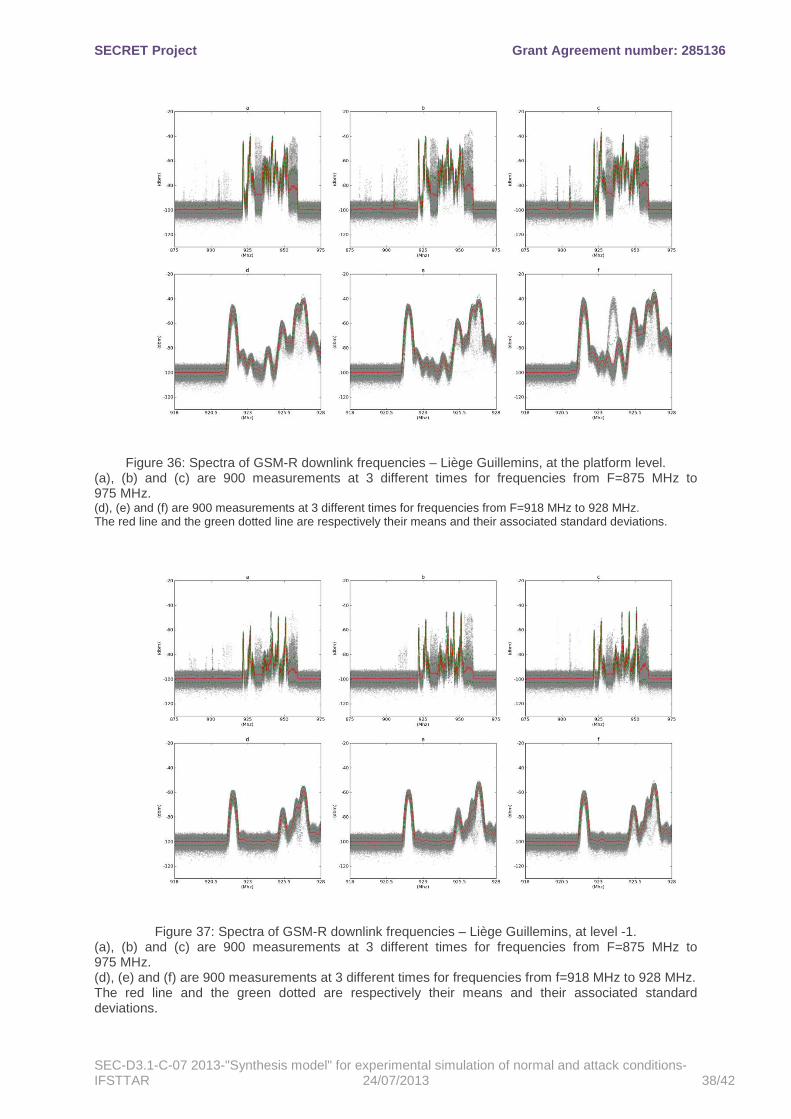
SECRET Project Grant Agreement number: 285136
SEC-D3.1-C-07 2013-"Synthesis model" for experimental simulation of normal and attack conditions-IFSTTAR 24/07/2013 38/42
Figure 36: Spectra of GSM-R downlink frequencies – Liège Guillemins, at the platform level. (a), (b) and (c) are 900 measurements at 3 different times for frequencies from F=875 MHz to 975 MHz. (d), (e) and (f) are 900 measurements at 3 different times for frequencies from F=918 MHz to 928 MHz. The red line and the green dotted line are respectively their means and their associated standard deviations.
Figure 37: Spectra of GSM-R downlink frequencies – Liège Guillemins, at level -1. (a), (b) and (c) are 900 measurements at 3 different times for frequencies from F=875 MHz to 975 MHz. (d), (e) and (f) are 900 measurements at 3 different times for frequencies from f=918 MHz to 928 MHz. The red line and the green dotted are respectively their means and their associated standard deviations.

SECRET Project Grant Agreement number: 285136
SEC-D3.1-C-07 2013-"Synthesis model" for experimental simulation of normal and attack conditions-IFSTTAR 24/07/2013 39/42
Figure 38: Spectra of GSM-R downlink frequencies – LGV Est, location 1. (a), (b) and (c) are 900 measurements at 3 different times for frequencies from F=875 MHz to 975 MHz. (d), (e) and (f) are 900 measurements at 3 different times for frequencies from F=918 MHz to 928 MHz. The red line and the green dotted line are respectively their means and their associated standard deviations.
Figure 39: Spectra of GSM-R downlink frequencies – LGV Est, location 2. (a), (b) and (c) are 900 measurements at 3 different times for frequencies from F=875 MHz to 975 MHz. (d), (e) and (f) are 900 measurements at 3 different times for frequencies from F=918 MHz to 928 MHz. The red line and the green dotted are respectively their means and their associated standard deviations.

SECRET Project Grant Agreement number: 285136
SEC-D3.1-C-07 2013-"Synthesis model" for experimental simulation of normal and attack conditions-IFSTTAR 24/07/2013 40/42
Firstly, we can observe that, for a same location, the mean and the standard deviation are relatively stable. However, if we observe these results more precisely and, if we compare the different sub-figures (a) (b) (c) between them (same exercise for (d), (e), (f)), we detect variations of the spectral means and of their standard deviations due to the presence of different signal to noise ratio. This distinction is more visible between F=875 MHz and F=920 MHz for the sub-figures (a) (b) and (c) (see another explicit example between the sub-figure 36(e) and sub-figure 36(f) for the band 918 MHz – 928 MHz). These variations are mainly due to the variability of the characteristics of communication signals (TDMA, FDMA...) or, basically, by the presence or absence of communication.
First conclusion: In a same location, the model of the EM environment should be able to represent correctly the temporal variations of the spectrum.
Secondly, if we consider the observations as a function of the location, we deduce different comportments of the EM environment. This observation is verified by comparing the corresponding figures of two different environments (station environment, versus LGV Est environment), see for example : Gare de L'Est figure 34 (or 35) and LGV Est figure 36 (or 37). In this context, two main factors can intervene: the difference of train density (-> more or less of EM perturbations and more or less of GSM-R communications) and the difference of civil communications density (-> more or less of GSM communications). For two same station environments but in different locations, variations are again present. For example, between figure 34 and figure 35 in Gare de l'Est (or figure 36 and figure 37 in Liège Guillemins). These figures show differences of power level in spectral channels modifying highly the spectral envelope. Moreover, in stations or along the LGV, the different location measurements imply differences of reception power in function of the location of BTSs (compare figure 34(d, e, f) with figure 35(d, e, f)) but also differences of number of received signals from distinct BTS (compare figure 36(d, e, f) with figure 37(d, e, f)).
Second conclusion: The model of the EM environment should able to repr esent correctly the locations variations of the spectrum.
Finally, all the figures show that the distribution of the samples (at each frequency) is not symmetric. The variation of each spectrum is more accentuated at the top that below the mean value (more visible for the stable frequencies). Therefore, the Gaussian distribution (symmetric by definition) cannot fit correctly these specific distributions of data measurements.
10.1.3. EM model : Intrinsic variations and variat ions in function of time
Although the estimation of the means and the standard deviations allows a prelimlinary understanding of the behavior of the EM environment, the hypothesis that the spectrum at each frequency follows a Gaussian process is restrictive. The first reason has been presented just before: for a frequency where the spectrum is stable, the distribution is not symmetric. Secondly, for a same location, the mean and the standard deviation can evolve differently as a function of time, this is mainly due to the variability of the communication signal at one frequency, the spectrum can be in two states : in communication (high level power) or not (low level power) (see figure 7). In these conditions, we propose to build a model using two states, one state corresponding to the presence of communication and one to the absence of communication. In the context of generative models, this can be modeled by a Gaussian mixture process. The expression of the Gaussian mixture model (GMM) is the following:
( )( ) ( )( )ggg
G
=gg ,σµ;fsNp=fsp ⋅∑
1
with:
1 101
=pandpG
=ggg ∑≤≤
and where Ng() is the gth Gaussian kernel defined by its mean and its standard deviation, G is the number of Gaussian kernel and pg weight of each Gaussian kernel in the mixture. The main idea is that one state is represented by one Gaussian kernel, but in our case the situation is more complex since for one stable state the distribution is not symmetric and therefore not Gaussian. Thus, more than two Gaussian kernels will be used, a dedicated number will be used for the state of absence of communication and another dedicated number will be used for the presence of communication.

SECRET Project Grant Agreement number: 285136
SEC-D3.1-C-07 2013-"Synthesis model" for experimental simulation of normal and attack conditions-IFSTTAR 24/07/2013 41/42
Figure 40: A sequence of 500 consecutive samples of the spectrum at the frequency f= 922 MHz. LGV Est, location 2.
10.1.4. EM Spectrum model: Variations in function t he location observation.
The last model will be able to model the variations in the time but not the variations due to different observation locations. We recall in this context that the spectra are different, due to the presence of different communication signals and/or at different power levels (BTS locations...) and/or the EM environment (difference of train density, difference of the propagation channels (multi-path) of the communication. In the light of this level of complexity, in a first time, our strategy is to build a statistical model for each location of observation. Once that these supervised models will be efficient, the goal will be to build semi-supervised models that will be able to evolve from one model to another one. For this, some a priori information can be determined and used, like the evolution of the power level of BTS in function of the distance, the distance between two BTS, the position of the BTS... If necessary, other a priori information will be estimated like the evolution of one complex EM environment to another one.
11. Conclusion
This D3.1 deliverable has focused on the evaluation of « normal » electromagnetic conditions in railway critical environments. Critical railway systems and sites have been identified and described. The methodology and the experimental conditions employed to collect reference noise conditions was described. Experimental results performed in European critical railway sites were reported. Theoretical techniques to determine a normal electromagnetic environment were presented and a preliminary analysis of the recorded experimental results was discussed.
12. Acknowledgements
The “Secret” involved team deeply thanks SNCF and SNCB for facilitating the in situ measurements presented in this Secret deliverable D3.1.

SECRET Project Grant Agreement number: 285136
SEC-D3.1-C-07 2013-"Synthesis model" for experimental simulation of normal and attack conditions-IFSTTAR 24/07/2013 42/42