Embed Size (px)
Citation preview
Math 53: Fall 2021, UC Berkeley Lecture 05 Copyright: J.A. Sethian
All rights reserved. You may not distribute/reproduce/display/post/upload any course materials in any way, regardless of whether or not a fee is charged, without my express written consent. You also may not allow anyone else to do so. If you do so, you will be prosecuted under UC Berkeley student proceedings Secs. 102.23 and 102.25 [email protected]
Section 14.1: Review of the Idea of Level Sets
Definition : Given f(x), we call the “k” level set the set of all inputs that get sent to the output value of k.
The level set lies in input space
1D Output space
f(x) = x2
Output = 9
Input = -3 Input = 3 1D Input space
1D Input space 1D Output space
Output = 9
f(x) = x2
Input = -3 Input = 3 The two elements of the f(x)=9 level set
Math 53: Fall 2021, UC Berkeley Lecture 05 Copyright: J.A. Sethian
All rights reserved. You may not distribute/reproduce/display/post/upload any course materials in any way, regardless of whether or not a fee is charged, without my express written consent. You also may not allow anyone else to do so. If you do so, you will be prosecuted under UC Berkeley student proceedings Secs. 102.23 and 102.25 [email protected]
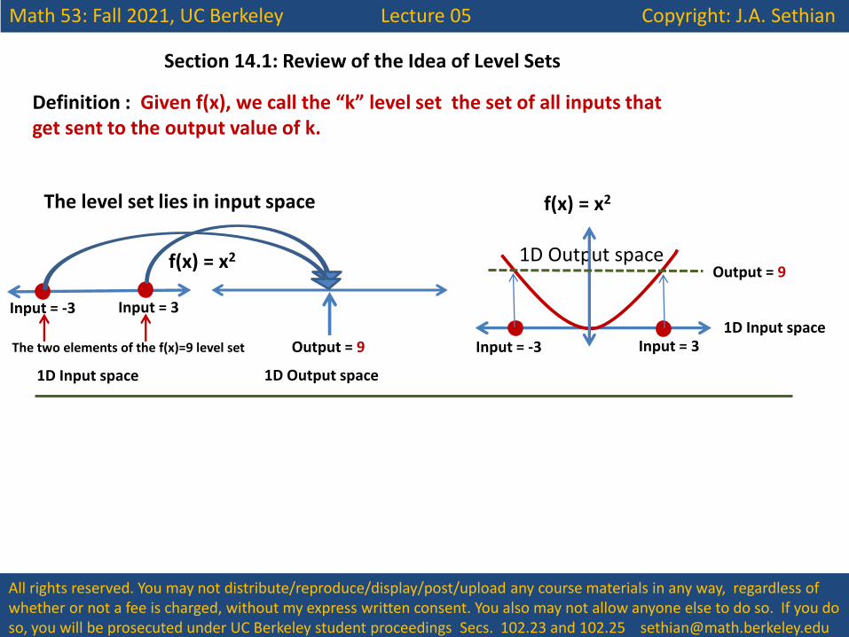
Section 14.1: Functions of Several Variables
f(x,y) = x2 + y2
x
y
z
What is the level set f(x,y) = 9?
2D Input space
Analytic answer: it is the set of all input points that get sent to the output 9 Geometric answer: if you slice the graph with a plane at height k, and project the result down to the input plane, the points you get are the k level set.
Level Set = 9: Circle of radius 3 in input
space
Output = at height z = 9
x
y
2D Input space
Level Set = 9: Circle of radius 3 in input
space
Output = at height z = 9 Slicing plane at
height z = 9
Level set is projection of intersection of surface with slicing plane onto input space
Math 53: Fall 2021, UC Berkeley Lecture 05 Copyright: J.A. Sethian
All rights reserved. You may not distribute/reproduce/display/post/upload any course materials in any way, regardless of whether or not a fee is charged, without my express written consent. You also may not allow anyone else to do so. If you do so, you will be prosecuted under UC Berkeley student proceedings Secs. 102.23 and 102.25 [email protected]
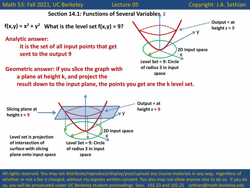
Section 14.1: Functions of Several Variables
Topo map from https://datavizproject.com/data-type/topographic-map/
And that’s what a topographic map is!
A topographic gives you different k-level sets in the input space, showing what the height of the earth would be. Contour lines show points of the same elevation.
x
y
z
2D Input space
1D Output space (height of the earth)
All sent to same height z = 230
230
So, if you walk along a level set in input space, your output does not change!
Math 53: Fall 2021, UC Berkeley Lecture 05 Copyright: J.A. Sethian
All rights reserved. You may not distribute/reproduce/display/post/upload any course materials in any way, regardless of whether or not a fee is charged, without my express written consent. You also may not allow anyone else to do so. If you do so, you will be prosecuted under UC Berkeley student proceedings Secs. 102.23 and 102.25 [email protected]
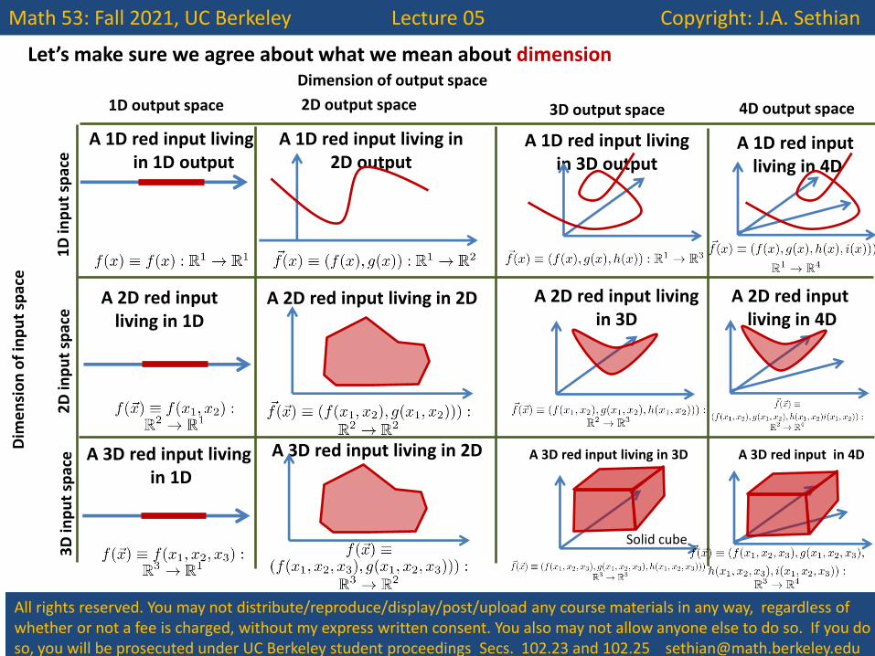
Let’s make sure we agree about what we mean about dimension
A 1D red input living in 1D output
A 1D red input living in 2D output
A 1D red input living in 3D output
A 1D red input living in 4D
A 2D red input living in 2D A 2D red input living in 3D
A 2D red input living in 4D
A 2D red input living in 1D
A 3D red input living in 2D A 3D red input living in 3D A 3D red input in 4D A 3D red input living in 1D
Solid cube
Dimension of output space
1D output space 2D output space 3D output space 4D output space
Dim
en
sio
n o
f in
pu
t sp
ace
1D
inp
ut
spac
e
2D
inp
ut
spac
e
3D
inp
ut
spac
e
Math 53: Fall 2021, UC Berkeley Lecture 05 Copyright: J.A. Sethian
All rights reserved. You may not distribute/reproduce/display/post/upload any course materials in any way, regardless of whether or not a fee is charged, without my express written consent. You also may not allow anyone else to do so. If you do so, you will be prosecuted under UC Berkeley student proceedings Secs. 102.23 and 102.25 [email protected]
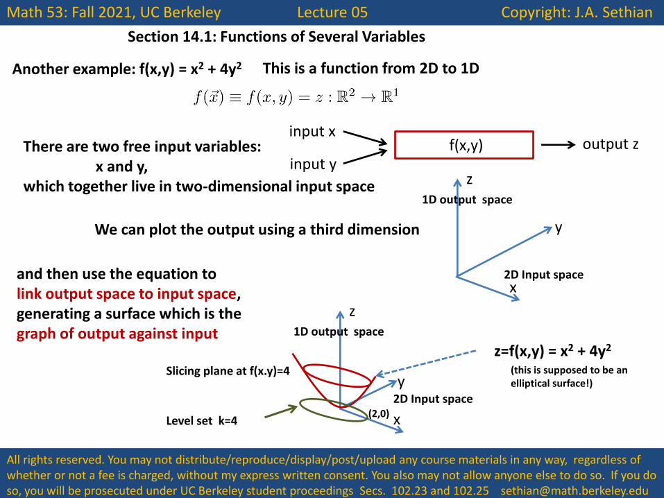
Section 14.1: Functions of Several Variables
Another example: f(x,y) = x2 + 4y2 This is a function from 2D to 1D
There are two free input variables: x and y, which together live in two-dimensional input space
f(x,y) input x
input y output z
We can plot the output using a third dimension
x
y
z
2D Input space
1D output space
and then use the equation to link output space to input space, generating a surface which is the graph of output against input
x
y
z
2D Input space
1D output space
z=f(x,y) = x2 + 4y2
(this is supposed to be an elliptical surface!)
Level set k=4 (2,0)
Slicing plane at f(x.y)=4
Math 53: Fall 2021, UC Berkeley Lecture 05 Copyright: J.A. Sethian
All rights reserved. You may not distribute/reproduce/display/post/upload any course materials in any way, regardless of whether or not a fee is charged, without my express written consent. You also may not allow anyone else to do so. If you do so, you will be prosecuted under UC Berkeley student proceedings Secs. 102.23 and 102.25 [email protected]
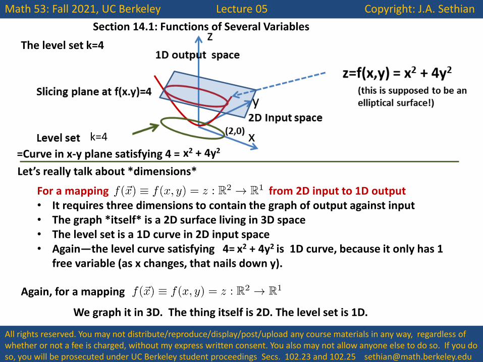
Section 14.1: Functions of Several Variables
=Curve in x-y plane satisfying 4 = x2 + 4y2
Let’s really talk about *dimensions*
For a mapping from 2D input to 1D output • It requires three dimensions to contain the graph of output against input • The graph *itself* is a 2D surface living in 3D space • The level set is a 1D curve in 2D input space • Again—the level curve satisfying 4= is 1D curve, because it only has 1
free variable (as x changes, that nails down y). x2 + 4y2
The level set k=4
Again, for a mapping
We graph it in 3D. The thing itself is 2D. The level set is 1D.
k=4
Math 53: Fall 2021, UC Berkeley Lecture 05 Copyright: J.A. Sethian
All rights reserved. You may not distribute/reproduce/display/post/upload any course materials in any way, regardless of whether or not a fee is charged, without my express written consent. You also may not allow anyone else to do so. If you do so, you will be prosecuted under UC Berkeley student proceedings Secs. 102.23 and 102.25 [email protected]
Section 14.1: Functions of Several Variables
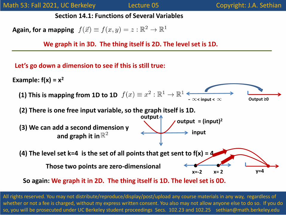
Again, for a mapping
We graph it in 3D. The thing itself is 2D. The level set is 1D.
Let’s go down a dimension to see if this is still true:
Example: f(x) = x2
(1) This is mapping from 1D to 1D Output ≥0 < input <
(2) There is one free input variable, so the graph itself is 1D. (3) We can add a second dimension y and graph it in (4) The level set k=4 is the set of all points that get sent to f(x) = 4
input
output output = (input)2
x=-2 x= 2 y=4 Those two points are zero-dimensional
So again: We graph it in 2D. The thing itself is 1D. The level set is 0D.
-
Math 53: Fall 2021, UC Berkeley Lecture 05 Copyright: J.A. Sethian
All rights reserved. You may not distribute/reproduce/display/post/upload any course materials in any way, regardless of whether or not a fee is charged, without my express written consent. You also may not allow anyone else to do so. If you do so, you will be prosecuted under UC Berkeley student proceedings Secs. 102.23 and 102.25 [email protected]
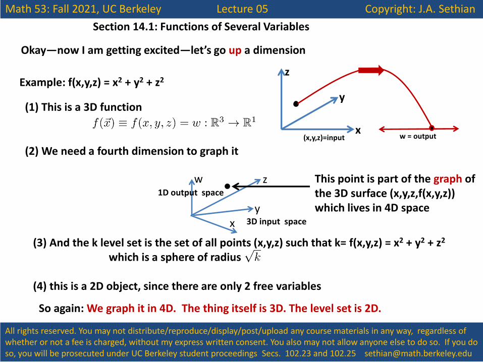
Section 14.1: Functions of Several Variables
Okay—now I am getting excited—let’s go up a dimension
Example: f(x,y,z) = x2 + y2 + z2
(1) This is a 3D function
x
y
z
w = output (x,y,z)=input
(2) We need a fourth dimension to graph it
x
z w 1D output space
y 3D input space
This point is part of the graph of the 3D surface (x,y,z,f(x,y,z)) which lives in 4D space
(3) And the k level set is the set of all points (x,y,z) such that k= f(x,y,z) = x2 + y2 + z2
which is a sphere of radius (4) this is a 2D object, since there are only 2 free variables
So again: We graph it in 4D. The thing itself is 3D. The level set is 2D.
Math 53: Fall 2021, UC Berkeley Lecture 05 Copyright: J.A. Sethian
All rights reserved. You may not distribute/reproduce/display/post/upload any course materials in any way, regardless of whether or not a fee is charged, without my express written consent. You also may not allow anyone else to do so. If you do so, you will be prosecuted under UC Berkeley student proceedings Secs. 102.23 and 102.25 [email protected]
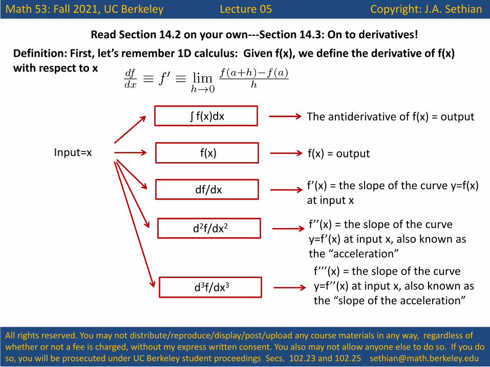
Read Section 14.2 on your own---Section 14.3: On to derivatives!
Definition: First, let’s remember 1D calculus: Given f(x), we define the derivative of f(x) with respect to x
ʃ f(x)dx
Input=x
The antiderivative of f(x) = output
f(x) f(x) = output
df/dx f’(x) = the slope of the curve y=f(x) at input x
d2f/dx2 f’’(x) = the slope of the curve y=f’(x) at input x, also known as the “acceleration”
d3f/dx3
f’’’(x) = the slope of the curve y=f’’(x) at input x, also known as the “slope of the acceleration”
Math 53: Fall 2020, UC Berkeley Lecture 05 Copyright: J.A. Sethian
All rights reserved. You may not distribute/reproduce/display/post/upload any course materials in any way, regardless of whether or not a fee is charged, without my express written consent. You also may not allow anyone else to do so. If you do so, you will be prosecuted under UC Berkeley student proceedings Secs. 102.23 and 102.25 [email protected]
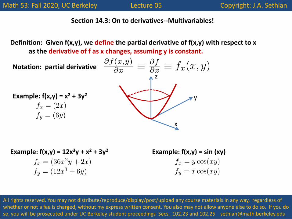
Section 14.3: On to derivatives--Multivariables!
Definition: Given f(x,y), we define the partial derivative of f(x,y) with respect to x as the derivative of f as x changes, assuming y is constant.
Notation: partial derivative
Example: f(x,y) = x2 + 3y2
x
y
z
Example: f(x,y) = 12x3y + x2 + 3y2 Example: f(x,y) = sin (xy)
Math 53: Fall 2020, UC Berkeley Lecture 05 Copyright: J.A. Sethian
All rights reserved. You may not distribute/reproduce/display/post/upload any course materials in any way, regardless of whether or not a fee is charged, without my express written consent. You also may not allow anyone else to do so. If you do so, you will be prosecuted under UC Berkeley student proceedings Secs. 102.23 and 102.25 [email protected]
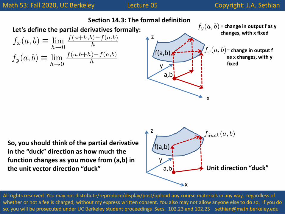
Section 14.3: The formal definition
Let’s define the partial derivatives formally:
x
y
z
a,b
= change in output f as x changes, with y fixed
= change in output f as y changes, with x fixed
f(a,b)
So, you should think of the partial derivative in the “duck” direction as how much the function changes as you move from (a,b) in the unit vector direction “duck”
x
y
z
a,b
f(a,b)
Unit direction “duck”
Math 53: Fall 2021, UC Berkeley Lecture 05 Copyright: J.A. Sethian
All rights reserved. You may not distribute/reproduce/display/post/upload any course materials in any way, regardless of whether or not a fee is charged, without my express written consent. You also may not allow anyone else to do so. If you do so, you will be prosecuted under UC Berkeley student proceedings Secs. 102.23 and 102.25 [email protected]
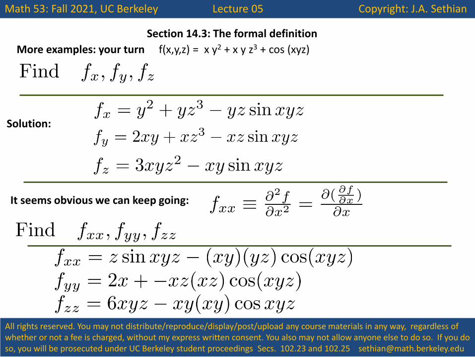
Section 14.3: The formal definition
More examples: your turn f(x,y,z) = x y2 + x y z3 + cos (xyz)
It seems obvious we can keep going:
Solution:
Math 53: Fall 2021, UC Berkeley Lecture 05 Copyright: J.A. Sethian
All rights reserved. You may not distribute/reproduce/display/post/upload any course materials in any way, regardless of whether or not a fee is charged, without my express written consent. You also may not allow anyone else to do so. If you do so, you will be prosecuted under UC Berkeley student proceedings Secs. 102.23 and 102.25 [email protected]
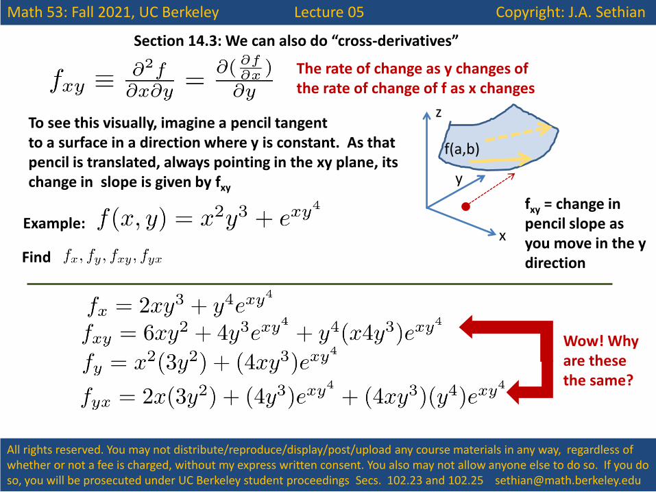
Section 14.3: We can also do “cross-derivatives”
The rate of change as y changes of the rate of change of f as x changes
To see this visually, imagine a pencil tangent to a surface in a direction where y is constant. As that pencil is translated, always pointing in the xy plane, its change in slope is given by fxy
x
y
z
f(a,b)
fxy = change in pencil slope as you move in the y direction
Example:
Find
Wow! Why are these the same?
Math 53: Fall 2021, UC Berkeley Lecture 05 Copyright: J.A. Sethian
All rights reserved. You may not distribute/reproduce/display/post/upload any course materials in any way, regardless of whether or not a fee is charged, without my express written consent. You also may not allow anyone else to do so. If you do so, you will be prosecuted under UC Berkeley student proceedings Secs. 102.23 and 102.25 [email protected]
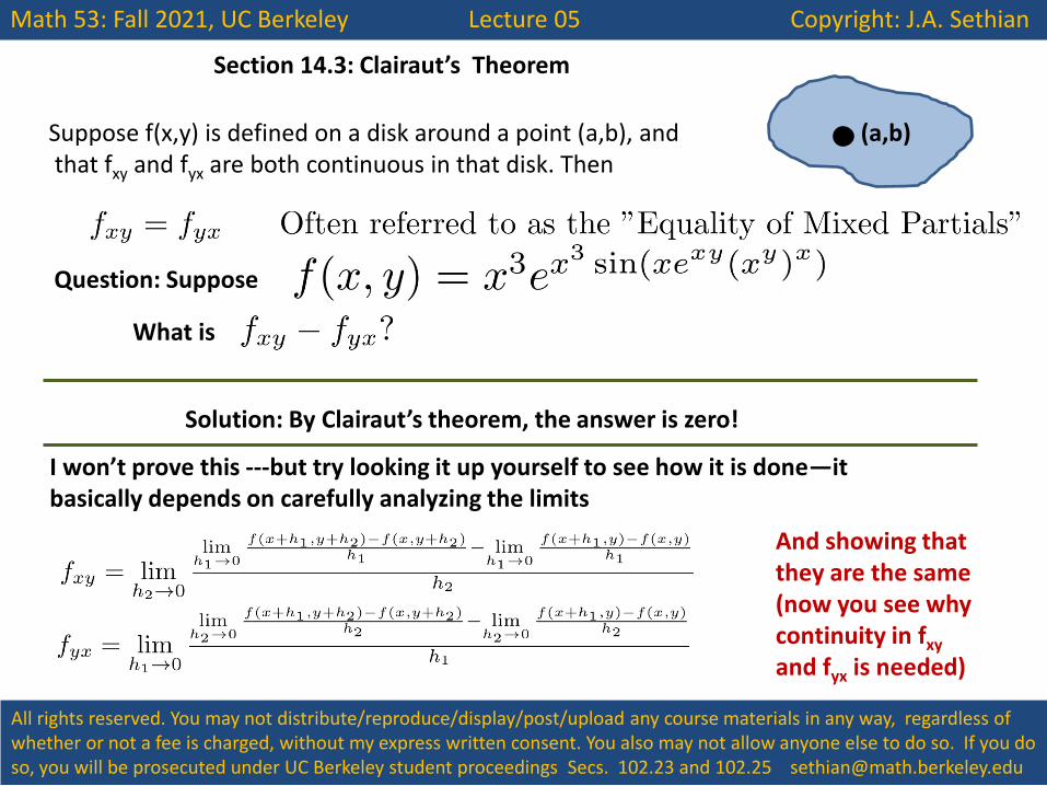
Section 14.3: Clairaut’s Theorem
Suppose f(x,y) is defined on a disk around a point (a,b), and that fxy and fyx are both continuous in that disk. Then
Question: Suppose
What is
Solution: By Clairaut’s theorem, the answer is zero!
(a,b)
I won’t prove this ---but try looking it up yourself to see how it is done—it basically depends on carefully analyzing the limits
And showing that they are the same (now you see why continuity in fxy and fyx is needed)
Math 53: Fall 2021, UC Berkeley Lecture 05 Copyright: J.A. Sethian
All rights reserved. You may not distribute/reproduce/display/post/upload any course materials in any way, regardless of whether or not a fee is charged, without my express written consent. You also may not allow anyone else to do so. If you do so, you will be prosecuted under UC Berkeley student proceedings Secs. 102.23 and 102.25 [email protected]
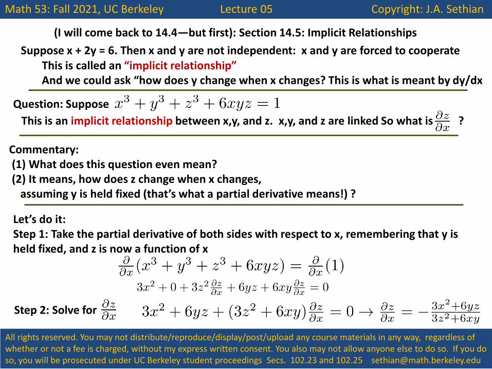
(I will come back to 14.4—but first): Section 14.5: Implicit Relationships
Question: Suppose
This is an implicit relationship between x,y, and z. x,y, and z are linked So what is ?
Suppose x + 2y = 6. Then x and y are not independent: x and y are forced to cooperate This is called an “implicit relationship” And we could ask “how does y change when x changes? This is what is meant by dy/dx
Commentary: (1) What does this question even mean? (2) It means, how does z change when x changes, assuming y is held fixed (that’s what a partial derivative means!) ?
Let’s do it: Step 1: Take the partial derivative of both sides with respect to x, remembering that y is held fixed, and z is now a function of x
Step 2: Solve for
Math 53: Fall 2021, UC Berkeley Lecture 05 Copyright: J.A. Sethian
All rights reserved. You may not distribute/reproduce/display/post/upload any course materials in any way, regardless of whether or not a fee is charged, without my express written consent. You also may not allow anyone else to do so. If you do so, you will be prosecuted under UC Berkeley student proceedings Secs. 102.23 and 102.25 [email protected]
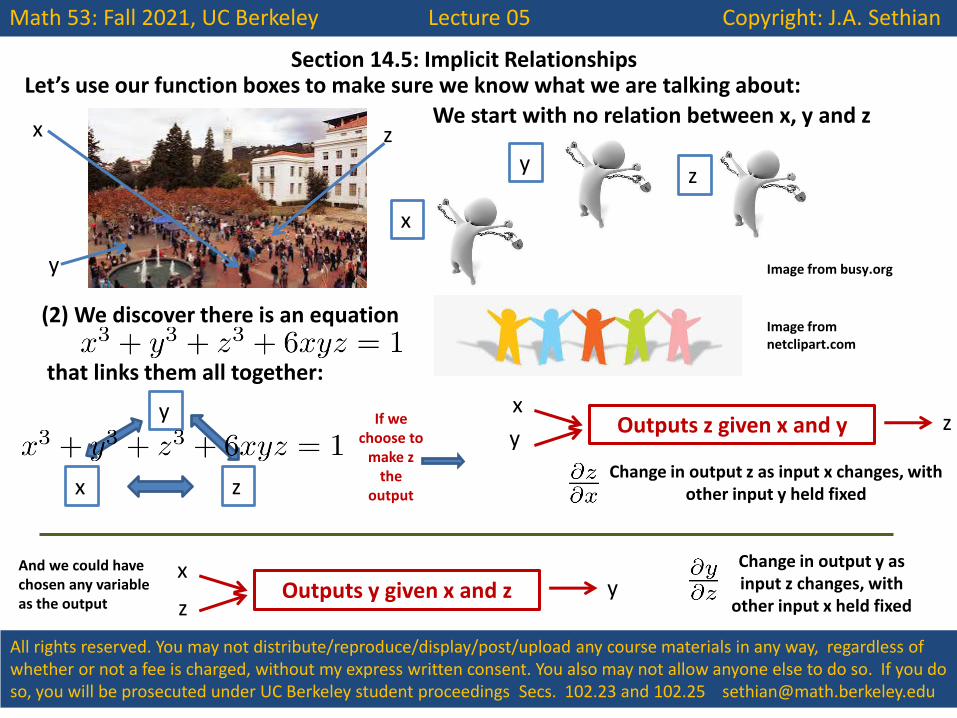
Section 14.5: Implicit Relationships Let’s use our function boxes to make sure we know what we are talking about:
x z
y
We start with no relation between x, y and z
x
y z
(2) We discover there is an equation that links them all together:
Image from busy.org
Image from netclipart.com
x
y z
x
y
z
Outputs z given x and y
Change in output z as input x changes, with other input y held fixed
And we could have chosen any variable as the output
x
z y Outputs y given x and z
Change in output y as input z changes, with
other input x held fixed
If we choose to
make z the
output
Math 53: Fall 2021, UC Berkeley Lecture 05 Copyright: J.A. Sethian
All rights reserved. You may not distribute/reproduce/display/post/upload any course materials in any way, regardless of whether or not a fee is charged, without my express written consent. You also may not allow anyone else to do so. If you do so, you will be prosecuted under UC Berkeley student proceedings Secs. 102.23 and 102.25 [email protected]
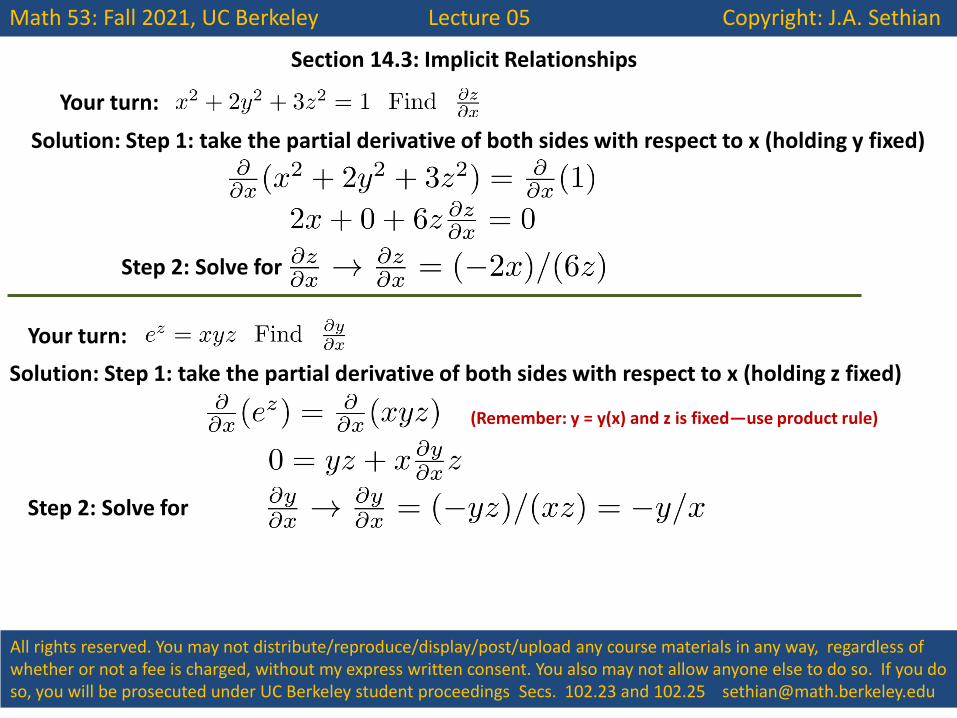
Section 14.3: Implicit Relationships
Your turn:
Solution: Step 1: take the partial derivative of both sides with respect to x (holding y fixed)
Step 2: Solve for
Your turn:
Solution: Step 1: take the partial derivative of both sides with respect to x (holding z fixed)
Step 2: Solve for
(Remember: y = y(x) and z is fixed—use product rule)
Math 53: Fall 2020, UC Berkeley Lecture 05 Copyright: J.A. Sethian
All rights reserved. You may not distribute/reproduce/display/post/upload any course materials in any way, regardless of whether or not a fee is charged, without my express written consent. You also may not allow anyone else to do so. If you do so, you will be prosecuted under UC Berkeley student proceedings Secs. 102.23 and 102.25 [email protected]
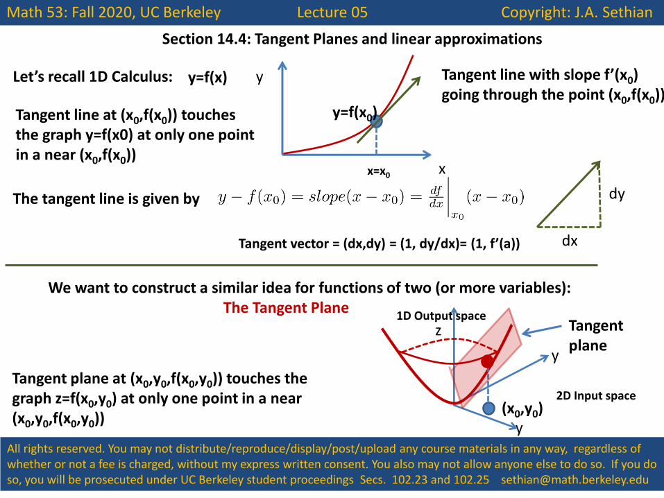
Section 14.4: Tangent Planes and linear approximations
Let’s recall 1D Calculus: y=f(x)
x
y
x=x0
y=f(x0)
Tangent line with slope f’(x0) going through the point (x0,f(x0))
The tangent line is given by
We want to construct a similar idea for functions of two (or more variables): The Tangent Plane
y
y
z
2D Input space
1D Output space
(x0,y0)
Tangent plane
Tangent line at (x0,f(x0)) touches the graph y=f(x0) at only one point in a near (x0,f(x0))
Tangent plane at (x0,y0,f(x0,y0)) touches the graph z=f(x0,y0) at only one point in a near (x0,y0,f(x0,y0))
dx
dy
Tangent vector = (dx,dy) = (1, dy/dx)= (1, f’(a))
Math 53: Fall 2020, UC Berkeley Lecture 05 Copyright: J.A. Sethian
All rights reserved. You may not distribute/reproduce/display/post/upload any course materials in any way, regardless of whether or not a fee is charged, without my express written consent. You also may not allow anyone else to do so. If you do so, you will be prosecuted under UC Berkeley student proceedings Secs. 102.23 and 102.25 [email protected]
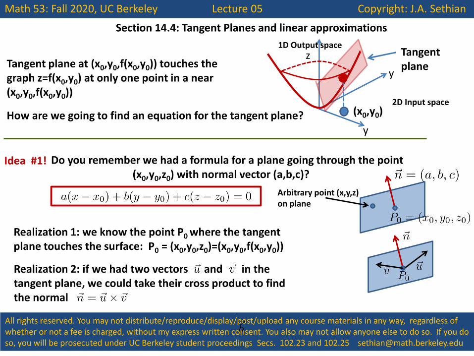
Section 14.4: Tangent Planes and linear approximations
y How are we going to find an equation for the tangent plane?
Idea #1! Do you remember we had a formula for a plane going through the point (x0,y0,z0) with normal vector (a,b,c)?
Arbitrary point (x,y,z) on plane
Realization 1: we know the point P0 where the tangent plane touches the surface: P0 = (x0,y0,z0)=(x0,y0,f(x0,y0))
y
z
2D Input space
1D Output space
(x0,y0)
Tangent plane Tangent plane at (x0,y0,f(x0,y0)) touches the
graph z=f(x0,y0) at only one point in a near (x0,y0,f(x0,y0))
Realization 2: if we had two vectors and in the tangent plane, we could take their cross product to find the normal
Math 53: Fall 2020, UC Berkeley Lecture 05 Copyright: J.A. Sethian
All rights reserved. You may not distribute/reproduce/display/post/upload any course materials in any way, regardless of whether or not a fee is charged, without my express written consent. You also may not allow anyone else to do so. If you do so, you will be prosecuted under UC Berkeley student proceedings Secs. 102.23 and 102.25 [email protected]
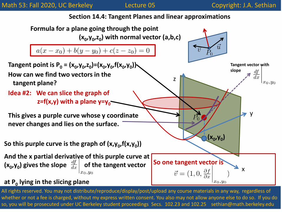
Section 14.4: Tangent Planes and linear approximations
Formula for a plane going through the point (x0,y0,z0) with normal vector (a,b,c)
Tangent point is P0 = (x0,y0,z0)=(x0,y0,f(x0,y0))
How can we find two vectors in the tangent plane?
Idea #2: We can slice the graph of z=f(x,y) with a plane y=y0
y
(x0,y0)
x
z
This gives a purple curve whose y coordinate never changes and lies on the surface.
So this purple curve is the graph of (x,y0,f(x,y0))
And the x partial derivative of this purple curve at (x0,y0) gives the slope of the tangent vector at P0 lying in the slicing plane
Tangent vector with slope
So one tangent vector is
Math 53: Fall 2020, UC Berkeley Lecture 05 Copyright: J.A. Sethian
All rights reserved. You may not distribute/reproduce/display/post/upload any course materials in any way, regardless of whether or not a fee is charged, without my express written consent. You also may not allow anyone else to do so. If you do so, you will be prosecuted under UC Berkeley student proceedings Secs. 102.23 and 102.25 [email protected]
Section 14.4: Tangent Planes and linear approximations
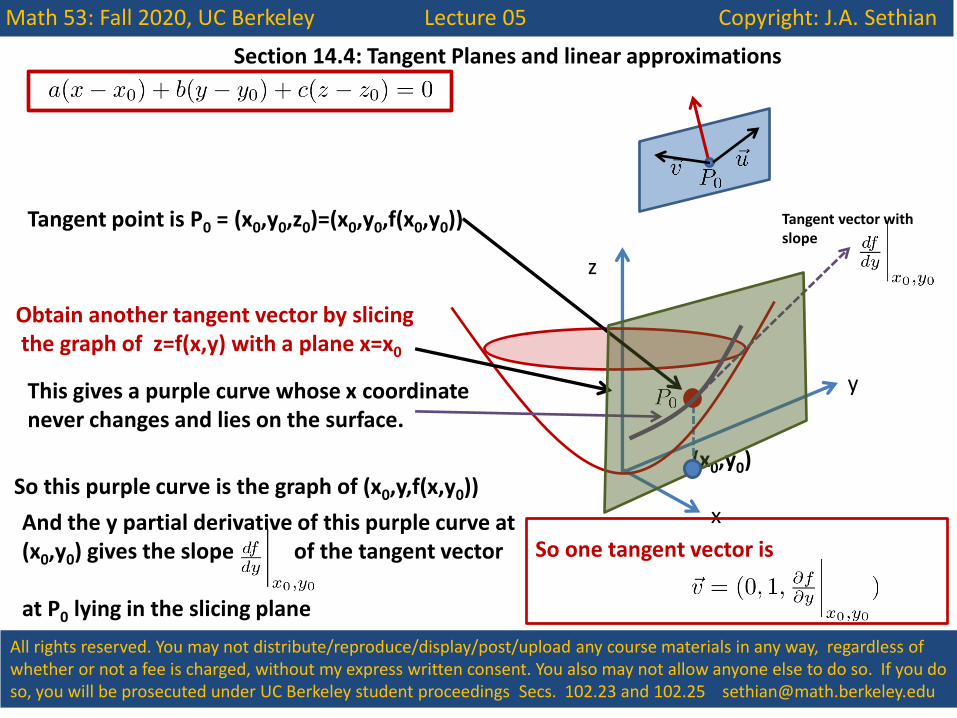
Tangent point is P0 = (x0,y0,z0)=(x0,y0,f(x0,y0))
Obtain another tangent vector by slicing the graph of z=f(x,y) with a plane x=x0
y
(x0,y0)
z
Tangent vector with slope
This gives a purple curve whose x coordinate never changes and lies on the surface.
x So this purple curve is the graph of (x0,y,f(x,y0))
And the y partial derivative of this purple curve at (x0,y0) gives the slope of the tangent vector at P0 lying in the slicing plane
So one tangent vector is
Math 53: Fall 2021, UC Berkeley Lecture 05 Copyright: J.A. Sethian
All rights reserved. You may not distribute/reproduce/display/post/upload any course materials in any way, regardless of whether or not a fee is charged, without my express written consent. You also may not allow anyone else to do so. If you do so, you will be prosecuted under UC Berkeley student proceedings Secs. 102.23 and 102.25 [email protected]
Section 14.4: Tangent Planes and linear approximations
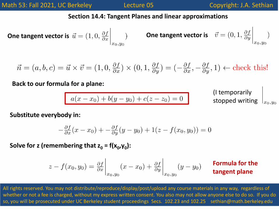
One tangent vector is One tangent vector is
Back to our formula for a plane:
Substitute everybody in:
Solve for z (remembering that z0 = f(x0,y0):
(I temporarily stopped writing
Formula for the tangent plane
Math 53: Fall 2021, UC Berkeley Lecture 05 Copyright: J.A. Sethian
All rights reserved. You may not distribute/reproduce/display/post/upload any course materials in any way, regardless of whether or not a fee is charged, without my express written consent. You also may not allow anyone else to do so. If you do so, you will be prosecuted under UC Berkeley student proceedings Secs. 102.23 and 102.25 [email protected]
Section 14.4: Tangent Planes and linear approximations
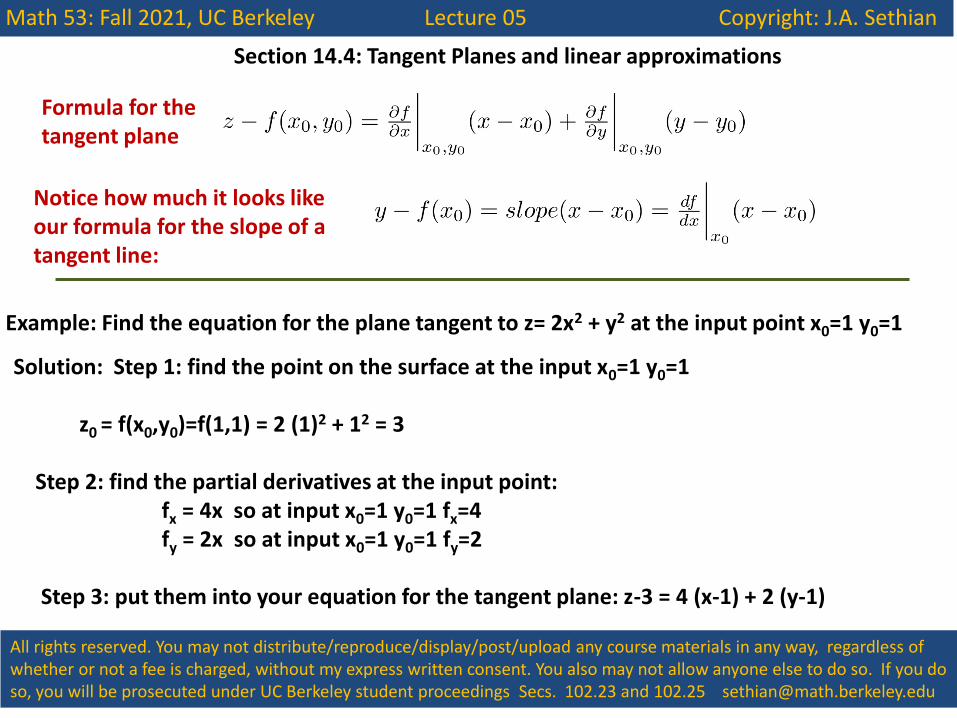
Formula for the tangent plane
Notice how much it looks like our formula for the slope of a tangent line:
Example: Find the equation for the plane tangent to z= 2x2 + y2 at the input point x0=1 y0=1
Solution: Step 1: find the point on the surface at the input x0=1 y0=1 z0 = f(x0,y0)=f(1,1) = 2 (1)2 + 12 = 3 Step 2: find the partial derivatives at the input point: fx = 4x so at input x0=1 y0=1 fx=4 fy = 2x so at input x0=1 y0=1 fy=2 Step 3: put them into your equation for the tangent plane: z-3 = 4 (x-1) + 2 (y-1)