Embed Size (px)
Citation preview

A spectral-domain approach for the calibration
of shot noise-based models of daily streamflows
Francesco Morlando
Dipartimento di Ingegneria Civile, Edile e Ambientale
A thesis submitted for the degree of
Ph.D. in Hydraulic and Environmental Engineering
Napoli, April 2015
Supervisors: Ph.D. Coordinator:
Prof. Domenico Pianese Prof. Elvira Petroncelli
Dr. Luigi Cimorelli
Dr. Luca Cozzolino


A Giuliano, Gianna, Maddalena, Alessia, Valeria ed Enrico
Siete stati sempre presenti. Vi voglio bene


Acknowledgements
The last three years at the Dipartimento di Ingegneria Civile, Edile e
Ambientale at the University of Napoli Federico II have been a fascinating
experience and I want to express my gratitude to some people that had a key
role in the development of my work.
First of all, I would like to thank Prof. Domenico Pianese, who has been
more than a mentor during the last years, teaching me the basics of being a
researcher and giving me the chance to express my capacities and aptitudes
autonomously.
A special thanks is needed to Dr. Luigi Cimorelli, who has been fundamental
in my growing process, supporting me in the resolution of a multitude of
complex problems until the night. Today we are friends and, as a friend, I
wish his dream of becoming a professor come true. He deserves the best.
I would also like to express my gratitude to Dr. Giovanni Mancini, member
of the Dipartimento di Ingegneria Elettrica e Tecnologie dell‟Informazione
at the University of Napoli Federico II, who introduced me to a completely
new scientific field, that of the system identification, with patient and high
competence.
Moreover, I would like to offer a special and sincere thanks to Prof. Alberto
Montanari. It was a honour for me to be guest, for a short period, of the
Dipartimento di Ingegneria Civile, Chimica, Ambientale e dei Materiali of
the University of Bologna and to have started such a stimulating

collaboration with one of the world‟s most notorious researcher in the
hydrologic field. I really hope to continue our research activities in the next
future and I would like, in particular, to thank him for his words of
appreciation for my skills and technical background.
A last, but not least, special thanks is for all my colleagues, friends and
especially my family, for all those laughs and for all the support that have
relieved my hardest days. Thank you all, guys.

Abstract
Since 50‟s the scientific community has been strongly interested in the
modeling of several classes of stochastic processes, among which a
particular attention has been attracted by hydro-meteorological phenomena.
Indeed, both their synthetic reproduction and forecasting is a central point in
the resolution of a wide class of problems, as the design and management of
water resources systems and flood risk analysis.
Concerning the modeling of generic stochastic variables, there are two
crucial aspects to be addressed: the identification of the most appropriate
model able to correctly reproduce the statistical features of the real process
(i.e., model selection), and the estimation of the parameters of the selected
model (i.e., model calibration) from available data, concerning both input
and output processes of the system to be identified.
During the last decades, considerable efforts have been undertaken by
researchers to provide the scientific community with suitable calibration
techniques of several class of models, resulting in the current availability of
numerous procedures for the estimation of the selected model parameters. A
general distinction can be made between time-domain and frequency-domain
(or spectral-domain) calibration approaches, whose main difference consists
in the typology of information adopted in the parameters estimation. Indeed,
while the former are usually based on a numerical comparison between
historical and synthetic series of the output process, spectral-domain

procedures adopt, in several ways, the frequency information content of
recorded input and output series. Such a substantial difference results in
some considerable advantages for frequency-domain techniques, especially
in the case of unavailability of sufficiently long and simultaneous records of
both input and output variables. This latter condition, in particular, is not rare
in the case of hydrologic model calibration problems, since the model input
sequences (e.g., rainfall and air temperature series) and the output sequence
(e.g., the streamflow series) can be usually both available but not
simultaneously or even unavailable (i.e., poorly gauged or ungauged basins).
These considerations make recommendable the adoption of frequency-
domain calibration techniques in hydrologic applications.
Starting from this proposed framework, in this thesis the author focuses on
the spectral-domain calibration problem of a widely developed class of
models for the modeling of daily streamflow processes, the so-called shot
noise models. These models consider the river flow process as the result of a
convolution of Poisson-distributed occurrences, representing the rainfall
process, and a linear response function, depending on the parameters to be
estimated, representing the natural basin transformations.
The technical literature provides several techniques for the calibration of this
class of models, both in the time and in the frequency domain. Nevertheless,
none of the existing procedures is found to take advantage of a remarkable
property of shot noise models, i.e. the impulsive nature of the autocorrelation
function of the input process. On the contrary, starting from this relevant
feature, the proposed calibration technique allow the estimation of the basin
response function parameters only through the knowledge of the power
spectral density of the recorded streamflow series. Hence, on the one hand,
the main drawbacks of classical time-domain calibration approaches are

solved and, on the other hand, the dependence of existing frequency-domain
techniques on the availability of both input and output data is overcome.
The effectiveness of the proposed procedure is widely proved through its
application to three daily streamflow series, associated to three watersheds
located in the Italian territory. In particular, performances of the approach in
the reproduction of the recorded flow series statistical properties are
ascertained through a simulation analysis.


i
Table of contents
List of figures .............................................................................................. v
List of tables .............................................................................................. vii
1. Introduction ............................................................................................. 1
2. State of the art ......................................................................................... 7
2.1. General aspects ................................................................................. 7
2.2. Brief survey of CT models identification methods ............................. 9
2.3. Parameter identification of linear CT models in the frequency-domain
.............................................................................................................. 15
3. Calibration of shot noise process-based models ..................................... 25
3.1. Introduction .................................................................................... 25
3.2. Reproduction of short time scale discharge series: a survey ............. 26
3.3. Shot noise models: main statistical properties.................................. 28
3.4. Shot noise models: classical calibration approaches ........................ 35
3.5. A spectral domain calibration procedure ......................................... 40
3.5.1. Model structure: the watershed response function ..................... 40
3.5.2. PSD estimation techniques ....................................................... 45

ii
3.5.2.1. A brief overview ................................................................ 45
3.5.2.2. Nonparametric (or conventional) methods .......................... 46
3.5.2.3. Parametric (or model-based) methods ................................ 47
3.5.3. The calibration approach ........................................................... 51
3.5.3.1. The parameters estimation.................................................. 51
3.5.3.2. Effective rainfall model selection and estimation ............... 57
3.6. Model validation and testing: a simulation analysis ......................... 62
4. Application and testing ........................................................................... 66
4.1. Description of the case studies streamflow series ............................. 66
4.2. Power spectral density (PSD) estimation ......................................... 72
4.3. Transfer function parameters estimation .......................................... 77
4.3.1. A multidimensional minimization approach: Powell‟s method .. 77
4.3.2. Calibration results ..................................................................... 79
4.4. Validation of the procedure: a simulation analysis ........................... 89
4.4.1. Synthetic effective rainfall series generation ............................. 89
4.4.1.1. Comparison between two methods for pulse sequence
derivation ....................................................................................... 89
4.4.1.2. PWNE model parameters estimation .................................. 99
4.4.2. Comparison of main statistical features between recorded and
synthetic streamflow series ............................................................... 101
4.4.2.1. Introduction ..................................................................... 101

iii
4.4.2.2. Comparison of mean statistics ......................................... 102
4.4.2.3. Comparison of flow-duration curves ................................ 106
4.4.2.4. Reproduction of minimum flow values over fixed durations
.................................................................................................... 111
5. Conclusions ......................................................................................... 117
5.1. Thesis summary ............................................................................ 117
5.2. Further developments .................................................................... 121
Appendix ................................................................................................. 123
References ............................................................................................... 127

iv
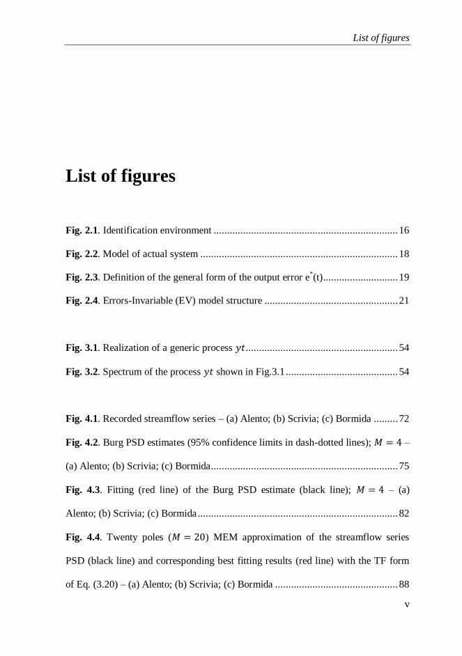
List of figures
v
List of figures
Fig. 2.1. Identification environment ..................................................................... 16
Fig. 2.2. Model of actual system .......................................................................... 18
Fig. 2.3. Definition of the general form of the output error e*(t) ............................ 19
Fig. 2.4. Errors-Invariable (EV) model structure .................................................. 21
Fig. 3.1. Realization of a generic process ......................................................... 54
Fig. 3.2. Spectrum of the process shown in Fig.3.1 .......................................... 54
Fig. 4.1. Recorded streamflow series – (a) Alento; (b) Scrivia; (c) Bormida ......... 72
Fig. 4.2. Burg PSD estimates (95% confidence limits in dash-dotted lines); –
(a) Alento; (b) Scrivia; (c) Bormida...................................................................... 75
Fig. 4.3. Fitting (red line) of the Burg PSD estimate (black line); – (a)
Alento; (b) Scrivia; (c) Bormida ........................................................................... 82
Fig. 4.4. Twenty poles ( ) MEM approximation of the streamflow series
PSD (black line) and corresponding best fitting results (red line) with the TF form
of Eq. (3.20) – (a) Alento; (b) Scrivia; (c) Bormida .............................................. 88

List of figures
vi
Fig. 4.5. Significant FPOT peaks in the first year of recording – (a) Alento; (b)
Scrivia; (c) Bormida ............................................................................................ 91
Fig. 4.6. Significant MA peaks in the first year of recording – (a) Alento; (b)
Scrivia; (c) Bormida ............................................................................................ 93
Fig. 4.7. Recorded and reconstructed runoff series comparison – (a) Alento; (b)
Scrivia; (c) Bormida ............................................................................................ 98
Fig. 4.8. Comparison of mean statistics of daily flows for each calendar month
between recorded (solid black line) and generated series (solid red line); confidence
intervals ±σ are shown in dashed line – (a) Alento; (b) Scrivia; (c) Bormida ....... 104
Fig. 4.9. Comparison between flow-duration curves of recorded (solid line) and
simulated (dotted line) series – (a) Alento; (b) Scrivia; (c) Bormida ................... 109
Fig. 4.10. Comparison of minimum mean discharges, averaged over different
durations, between recorded (circle points) and synthetic (cross points) series with ±
2σ confidence limits (dotted points) – (a) Alento; (b) Scrivia; (c) Bormida ......... 114

List of tables
vii
List of tables
Tab. 4.1. Characteristic features of drainage basins and runoff series considered in
the application ..................................................................................................... 67
Tab. 4.2. Estimated parameters of the watershed TF of Eq. (3.20) ........................ 80
Tab. 4.3. Estimated parameters of the watershed TF of Eq. (4.5) .......................... 83
Tab. 4.4. Comparison of spectral and time-domain parameters estimates ............. 85
Tab. 4.5. goodness-of-fit test for non-homogeneous Poisson distribution on
significant MA peaks ........................................................................................... 94
Tab. 4.6. Mean number of rainfall events per year: comparison between MA and
FPOT procedures ................................................................................................. 95
Tab. 4.7. PWNE model parameters estimates ..................................................... 100
Tab. 4.8. Recorded and mean synthetic flow volumes comparison for each case
study series ........................................................................................................ 106


Section 1. Introduction
1
1. Introduction
Stochastic modeling of hydro-meteorological phenomena has always been
attracting a great interest among the scientific hydrologic community,
especially given the relevant interest in the generation of synthetic data that
represent non-deterministic inputs to the generic system under study, thus
providing a basis for undertaking a variety of water-related design,
operation, and diagnostic studies. Indeed, synthetic data generation allows
accounting for uncertainty and large variability of input into the related
process. Several technical fields are strongly suitable for the implementation
of such approaches, due to the intrinsically uncertain nature of hydro-
meteorological phenomena involved, as input processes, into the problem to
be solved. Moreover, the use of synthetic time series, instead of historical
records, is essential for providing sufficiently large samples (e.g., with
length of hundreds or thousands of years) in order to evaluate a wide range
of possible outcomes [Efstratiadis et al., 2014].
One could think, for instance, to design and management problems of water
resources systems, as the necessity of determining the most effective
scheduling of an artificial reservoir over a fixed time period, in terms of
maximization of system reliability (namely the probability of satisfying the
associated water uses and constraints). In these cases the generation of
Section 1. Introduction
2
streamflow series from weekly to monthly aggregation scale is usually
required. Moreover, for the representation of streamflows, finer time steps
are also adopted (e.g., daily), for taking into account reservoir spills [Ilich,
2014] and small-scale regulations. Another field of application of stochastic
approaches involves the evaluation of flood risk, which requires even more
detailed temporal resolutions (e.g., hourly). In particular, during the last
years, a considerable attention has been paid to continuous flood modeling
which makes use of synthetic rainfall [Boughton and Droop, 2003].
Synthetic weather data (i.e., temperature, potential evapotranspiration, solar
radiation, wind velocity, etc.), can result particularly interesting in a wide
range of water, energy and environmental applications, including the design
and management of renewable energy systems [Tsekouras and
Koutsoyiannis, 2014]. Furthermore, other several technical problems can be
thought to be solved by the adoption of synthetic generator of river flows, as
the evaluation of the long-time effects of erosion phenomena of river banks
in a given section of interest, or the evaluation of the most convenient
nominal power of a new hydropower system to be designed.
The basic features of hydrologic time series that a stochastic model should
be able to correctly reproduce can be summarized as [Efstratiadis et al.,
2014]:
(1) asymmetric and marginal probability distribution;
(2) persistent large amplitude variations at irregular time intervals and
frequency-dependent amplitude variations;
(3) periodicity, which appears at the sub-annual scale (e.g., monthly) and is
due to the Earth motion;
(4) intermittency, which is a key feature of several processes at fine temporal
scales (e.g., daily rainfall and discharges) and which is quantified by the
probability that the value of the process within a time interval is zero (often

Section 1. Introduction
3
referred to as probability dry). Intermittency also results in significant
variability and high positive skewness, which are difficult to reproduce by
most generators.
Starting from these relevant properties, the scientific literature has provided,
during the last decades, several models for the generation of synthetic
hydrologic time series. Among others, it is worth reporting the following:
shot noise model [Weiss, 1977], fragment model [Srikanthan and McMahon,
1980], AutoRegressive Moving Average (ARMA) model [Box et al., 1994],
Artificial Neural Networks (ANNs) [Raman and Sunilkumar, 1995],
stochastic disaggregation model [Valencia and Schaake, 1973], Markov
chain model [Aksoy, 2003], bootstrapping method [Lall and Sharma, 1996]
and wavelets [Bayazit and Aksoy, 2001].
A considerable ability in the reproduction of hydrologic series, in particular
river flow time series, considering a short-time scale (from daily to weekly),
belongs to the aforementioned shot noise models, introduced by Bernier
[1970]. Several hydrologic literature works have dealt with the adoption of
this class of models for the reproduction of streamflow process main features
[Weiss, 1977; Murrone et al., 1997; Xu et al., 1997; Xu et al., 2002; Claps
and Laio, 2003 etc.], considering a shot noise process as input of a linear
system that represents the watershed physical features.
Furthermore, several techniques have been introduced for the calibration
(i.e., the estimation of the model parameters value) of shot noise-based
models [Kelman, 1980; Koch, 1985; Murrone et al., 1997; Xu et al., 2002;
Claps et al., 2005]. Most of the existing approaches, in particular, are based
on a time-domain procedure, consisting in a minimization of a cost function
given by the sum of the differences between recorded and generated
streamflow values. Such an approach, however, is conditioned by the high

Section 1. Introduction
4
availability of input/output recorded data, which can limit their adoption in
the so-called ungauged basins (i.e., those basins with a limited availability of
input and/or output data).
Several recent contributions have dealt with calibration problems in case of
ungauged basins. Some authors have discussed about the regionalization of
rare hydrologic information [Bloeschl and Sivapalan, 1995; Post and
Jakeman, 1999 and Parajka et al., 2005, among others]. Seibert and
McDonnell [2002], instead, investigated on the adoption of soft-data, which
are qualitative and/or scattered records.
A further valid alternative to time-domain approaches is that offered by
frequency-analysis of available input and output records, since spectral
features contain information that are not obtainable by raw time series and
that can be adopted to simplify the calibration procedure. A recent
interesting contribution in this direction was that of Quets et al. [2010], who
provided an interesting comparison between time and frequency-domain
approaches. In general, several frequency-domain techniques have been
introduced in the last years for the calibration of conceptual hydrologic
models [Labat et al., 2000; Kirchner et al., 2000; Islam and Sivakumar,
2002; Schaefli and Zehe, 2009 etc.]. Among them, a great interest has been
attracted by the methodology introduced by Montanari and Toth [2007] (and
subsequently adopted by Castiglioni et al. [2010]), who adopted the
maximum likelihood estimator introduced by Whittle [1953], for the
estimation of non-linear hydrologic models, from the only knowledge of
input and output data power spectral density estimations. In particular the
authors underlined how power spectral estimates could be achieved in
absence of numerous and simultaneous input/output data records., thus
assessing the usefulness of spectral-domain calibration techniques also in

Section 1. Introduction
5
presence of ungauged basins. Furthermore, starting from the pioneering
work of Pegram [1980], in the last decades a relevant contribution to the
spectral calibration of shot-noise based models has been developed [Diskin
and Pegram, 1987]. In this Ph.D. thesis, the parameters, of a hydrologic
conceptual linear model, were estimated through the minimization of a cost
function, given by the difference between the Laplace transform of the
historical and simulated streamflow series. However, to allow the application
of the whole procedure, the authors clearly took into account the different
structures of input and output sequences, following the previous contribution
of Diskin [1964].
Starting from this framework, the main aim of the present dissertation is the
description of a spectral-domain approach for the calibration of shot noise-
based models of streamflow processes. The whole work has to be intended
as an advance of the works of Murrone et al., 1997 and Claps et al., 2005,
who both adopted different time-domain procedures for the calibration of a
lumped-conceptual effective rainfall-runoff model, for streamflow modeling,
given by the series/parallel linear combination of linear reservoirs. The same
simplified hydrological model has been adopted in the present thesis, since
the central issue deals with the introduced calibration procedure, which, by
taking advantage of a relevant spectral property of shot noise-based models,
can allow the model calibration only by the availability of streamflow data
(so, useful in the case of ungauged basins).
The thesis has been structured as follows.
In Section 2 (i.e., State of the Art), a comprehensive, but also synthetic,
overview of time and frequency-domain, continuous time, calibration
techniques of linear time invariant systems is provided.

Section 1. Introduction
6
Section 3 (i.e, Identification of shot noise process-based models) firstly
provides a survey on the available models for the reproduction of short time
scale discharge series. Among them, subsequently, a focus on the main
properties of shot noise-based models is given, with the successive
description of their classical calibration techniques, both in the time and in
the frequency domain. Finally, the proposed calibration technique is deeply
described, providing details on the techniques for the estimation of the
power spectral density of the streamflow process and, moreover, on the
selection and the estimation of the effective rainfall model, fundamental for
the simulation analysis to be undertaken for the model validation and testing
phase.
In Section 4 (i.e., Application and testing), the overall calibration procedure
is applied to three case-study Italian watersheds, whose characteristics, both
in physical and climate terms, are provided in the first part of the section.
Subsequently, once estimated the unknown response function parameters,
results of several validation tests are provided, both in numerical and
graphical form, in order to assess the effectiveness of the whole procedure.
In Section 5 (i.e., Conclusions), the most important achieved results are
synthetically provided.
Eventually, the author provides the reader with an appendix, in order to
allow the complete understanding of the numerous spectral analysis concepts
that have been introduced in the whole thesis.

Section 2. State of the art
7
2. State of the art
2.1. General aspects
The main goal of the present Ph.D. dissertation deals with the development
of a spectral-domain identification technique of linear dynamic, conceptually
based, continuous and time invariant models of daily river flows. In
particular, the author focused his work on shot noise process-based models,
deeply discussed in Section 3 of the present thesis.
In order to give to the reader the tools to understand the developed topic, in
the present section a complete and synthetic description of time-domain
identification techniques of linear Continuous Time (CT) invariant models is
firstly provided. Secondly, frequency-domain identification procedures are
analyzed in detail.
In the system identification field, the identification of linear CT Time
Invariant (TI) models was one of the first objectives pursued by the scientific
community. In particular, in order to assess the parameters value of a generic
CT model, the technical literature provides two distinct class of approach: an
indirect and a direct technique. In the former, the sampled data of input and
output processes are adopted in the identification procedure of a Discrete

Section 2. State of the art
8
Time (DT) model, which is after converted in an equivalent CT model. In
the latter, instead, a direct estimate of the CT model parameters is
undertaken, without considering the equivalent DT model.
Several authors have discussed about advantages and disadvantages of the
two approaches. In particular, Rao and Unbehauen [2006] and Young and
Garnier [2006] propose an interesting survey about this topic, providing
some highlights, summarized hereinafter, on the reasons why one should
prefer a CT modeling to a DT one.
First of all, CT will always remain the natural basis of our understanding of
the physical world, because all the physical laws (Newton‟s, Faraday‟s etc.)
are in CT, with no chances of being rewritten in DT.
Secondly, the process of discretization itself is associated with some
undesirable consequences. In general, a strictly proper CT rational Transfer
Function (TF), , with poles, transformed into its equivalent discrete
expression, , through the well-known relations between the Laplace
plane (represented by the Laplace variable, ) and the z-transform plane,
remains rational and possesses generically zeros that cannot be
expressed in closed form in terms of the s-plane parameters and the sampling
time (for further details the reader can refers to Rao and Unbehauen
[2006]).
Thirdly, discretization may turn a native minimum phase CT model into a
problematic one with non-minimum phase properties. As a matter of fact, as
deeply described in Section 3, the identification procedure for the latter class
of models is more problematic if compared to the former class.
Furthermore, the fourth problem, listed by Rao and Unbehauen [2006] in
their work, deals with the fact that discretization gives rise to undesirable
sensitivity problems at high sampling rates, that is parameters value are
dependent on the adopted sampling intervals of the input and output data.

Section 2. State of the art
9
Finally, and perhaps most importantly, CT models can be identified and
estimated from rapidly sampled data, whereas DT models encounter
difficulties when the sampling frequency is too high in relation to the
dominant frequencies of the system under study [Astrom, 1969]. In this
situation, the eigenvalues lie too close to the unit circle in the complex
domain and the discrete-time model parameter estimates become statistically
ill-defined. The practical consequences of this are:
- either that the discrete-time estimation fails to converge properly, thus
providing an erroneous explanation of the data;
- or that even if convergence is achieved, the continuous-time model, as
obtained by standard conversion from the estimated discrete-time model,
does not provide the correct continuous-time model.
From these considerations it should be evident the convenience of the
adoption of the direct procedure in the identification of a CT and TI models,
avoiding, in this manner, the step corresponding to the identification of an
equivalent DT model. As a consequence, in the following part of the present
section, a detailed review of only CT identification techniques, available in
the scientific literature, is provided.
It is worth noticing that for further details on some of the concepts treated in
this section (e.g., the concept of TF of a linear model, poles and zeros of the
TF etc.), the interested reader can refer to Appendix.
2.2. Brief survey of CT models identification methods
The theoretical basis for the statistical identification and estimation of linear,
continuous-time models from DT sampled data can be outlined by
considering the following Single-Input, Single-Output (SISO) system:

Section 2. State of the art
10
(2.1)
(2.2)
where is any pure time delay in time units, the ratio ⁄ is
the system TF, and e are the following polynomials in the
derivative operator ⁄ :
(2.3)
(2.4)
This transfer function model (TFM) structure is denoted by the triad [n, m,
τ]. In Eq. (2.1), is the input signal, is the „noise free‟ output signal
and is the noisy output signal. In the following of the dissertation, the
assumption of zero mean White Noise (WN) with Gaussian amplitude
distribution for the noise term is considered, for the sake of simplicity,
even though this is not a restrictive assumption. The two series of
coefficients and are the sets of the model parameters to estimate.
By the principle of superposition for linear systems, is a vector of
stochastic disturbances which accounts for the combined effect of the input
and output disturbances at the output of the system. Although the nature of
this disturbance vector is not necessarily specified, it is often considered, for
analytical purposes, to have rational spectral density and so to be described
by the following Auto Regressive-Moving Average (ARMA) model:
(2.5)

Section 2. State of the art
11
where the ratio between the two polynomials and is the
disturbance TF, , while is a zero mean, serially uncorrelated, WN
CT process.
Once analytically defined the model structure, given by Eqs. (2.1) and
(2.2), it now possible to provide the model identification approach. The most
obvious approach to the estimation of the parameters in a mathematical
model, of a dynamic system, is to minimise a scalar cost (or loss) function ,
which is formulated in terms of some norm in an error function, , which
reflects the discrepancy between the output of the model and the real
system [Young, 1981]. It is the choice of which most differentiates the
various estimation methodologies which have been developed over the past
fifty years and this is discussed in detail in this subsection.
Concerning the choice of the cost function , instead, the most common is
given by the following relation:
∑ ‖ ‖
(2.6)
where the subscript indicates the value of the vector at the ith
sampling instant, denotes the number of samples available in the
observational interval and is the vector of the weights to associate to each
of the components of the vector .
Starting from previous considerations, the following part of the present
subsection is aimed at the short description of the several approaches for the
CT model identification. It is worth noticing that following procedures
differ, between each other, for the error function chosen in the
definition of the cost function of Eq. (2.6).

Section 2. State of the art
12
The first proposed approach is known as Output Error (OE) or Response
Error (RE) method and it is probably the most intuitively one to the problem
of system parameter estimation. Here, the parameters are chosen so that they
minimise either an instantaneous (in the purely deterministic case
corresponding to the condition ) or an integral (in the stochastic
case) norm in the error between the model output, denoted by , and the
observed output , i.e. with the following model error expression
. In the SISO case system of Eqs. (2.1) and (2.2), for
instance, the error function is defined as:
(2.7)
where and are, respectively, the estimates of the polynomials and
that define together the TF of the system to be identified.
The second approach is known as Equation Error (EE) method and clearly
derives from an analogy with statistic regression analysis. Here, the error
function is generated directly from the input-output equations of the model.
In particular, considering the previously defined model , a scalar error
function is involved and it is defined as follows:
(2.8)
The reader will certainly note that such a definition of the error function
implies the time derivatives of the input and output process [Eykhoff, 1974].
See, for evidence, Eqs. (2.3) and (2.4) defining expressions of the
polynomials and . It is worth noticing that in the deterministic case

Section 2. State of the art
13
(i.e. when the noise level of the measured input and output signals is low,
that means with a noise/signal ratio < 5%), the (2.8) is a linear algebraic
function of the unknown parameters; as a consequence, its minimization is
much more straightforward than in the OE case. For this particular case,
several EE schemes have been proposed in the scientific literature both for
linear and nonlinear systems, and most are mentioned by [Eykhoff, 1974].
Nevertheless, the inherent limitations of the deterministic approach soon
became apparent and many researchers suggested different solutions which
were not so sensitive to stochastic disturbances of the signals. In particular,
two were the main problems deriving from a deterministic approach applied
to noisy signals:
- the differentiation of signals possibly affected by noise (“noisy signal”);
- the asymptotic bias in the parameters estimation.
An alternative Generalized Equation Error (GEE) method is often defined to
avoid the obvious problems that arise from the differentiation of noisy
signal. Here, the input and output signal are passed through a State Variable
Filter (SVF) set, denoted by , which simultaneously filters the signal
and provides filtered time derivatives [Young, 1964], which replace the exact
but unobtainable derivatives in the definition of a modified version of .
Furthermore, the simplest solution to the asymptotic bias problem associated
with the basic EE approach is the Instrumental Variable (IV) method. Here
the least squares solution is modified to include a vector of instrumental
variables, , which are chosen in order to be highly correlated with the
noise-free output of the system, but totally uncorrelated with the noise on
the measurements of the system variables [Young, 1981].
Subsequently, the Refined IV (RIV) method, suggested by Young [1976],
was introduced. It is a similar but more sophisticated IV procedure, which is

Section 2. State of the art
14
able to achieve asymptotic statistical efficiency by the introduction of
adaptive “prefilters” on all the measured signals [Young, 1981].
The third reported approach is the Prediction Error (PE) method. Here, as in
the OE case, the error function is usually defined as , but
with | . As a matter of fact, in this case is defined as some
best prediction of , given the current estimates of the parameters a that
characterize the system and the noise models. In other words, | is the
conditional mean of given all current and past information on the
system. In the SISO case of model , the most obvious PE method involves
the minimization of a norm in , defined as:
*
+ (2.9)
where polynomials and define the noise model to sum to the output of
the real system [Solo, 1978].
Of course other arrangements are possible for a PE error function definition,
for example defining the error function within an EE context. For the sake of
conciseness this scheme is not reported here, but one can surely state that the
solution of the PE minimization problem is generally more complex than the
OE and EE equivalents, since the formulation of the PE norm implies the
concurrent estimation of the noise model parameters [Young, 1981].
The fourth reported approach can be considered as a particular case of the
PE minimization and it is known as Maximum Likelihood (ML) method. It
is considered separately here, however, because of its importance as a
motivating concept in research. The ML approach is based on the definition

Section 2. State of the art
15
of a PE type error function, but the formulation is restricted by the additional
assumption that the stochastic disturbances to the system have specified
amplitude probability distribution functions [Stepner and Mehra, 1973;
Kallstrom et al., 1976]. In particular, in most applications, this assumption is
restricted further for analytical tractability to the case of a Gaussian
distribution, in which case, the ML formulation coincides with certain PE
formulations.
The ML method can often be extended so that a priori information on the
probability distributions is included in the formulation of the problem. This
is termed the Bayesian (B) approach, since it arises from Bayes rule for
linking a priori to a posteriori probability statements and, so, allows for the
inclusion of a priori information into the solutions of the estimation
problem. Further details about this approach can be found in Young [1981].
2.3. Parameter identification of linear CT models in the frequency-
domain
Model parameters estimation in the frequency-domain is of considerable
interest because of its convenience in many practical situations. Information
on the system behaviour under the influence of periodic test signals is the
main input to spectral-domain identification algorithms. Identification in
frequency-domain is discussed, in the present subsection, with reference to
linear CT systems of the typology shown in Fig. 2.1., where and
are measurable input and output signals respectively, with the output signal
corrupted by the coloured immeasurable noise signal .

Section 2. State of the art
16
Fig. 2.1. Identification environment
A system is generally represented by its frequency-response characteristic
(Nyquist plot or its equivalent Bode plot):
(2.10)
This information may be available at discrete frequency values, ,
distributed, for example, logarithmically over the frequency range of
interest, from computation or by direct measurement. and are
the Fourier transforms of and , respectively, while and
are, respectively, real and imaginary part of the complex system
response function.
Measurements (or equivalently estimates) of , for discrete values of
covering the whole frequency range, can be obtained either [Rao e
Unbehauen, 2006]:
(a) from a discrete set of measured input-output spectra and for
, or
(b) from direct excitation by periodic test signals, or
(c) indirectly from arbitrary time-domain measurements of and ,
which, by Fourier transformation, convert the information into the
frequency-domain.

Section 2. State of the art
17
Concerning the latter case, in particular, two main TF estimation methods
are available in the literature, starting from recorded input and output signal.
The first one deals with the so called Empirical Transfer Function Estimate
(ETFE), given by the quotient between the Fourier transform of output and
input signal [Ljung, 1987, Subsection 6.3]. The second one, instead, consists
in the ratio between the input/output Cross-Power Spectral Density (CPSD)
and the input Power Spectral Density (PSD) estimations [Broersen, 1995].
Even though the aim of the author is not that of focusing on a detailed
description of TF estimator, it is worth noticing a fundamental feature of
CPSD estimators, that is their ability in preserving both magnitude and phase
information of the system frequency response. As a consequence, such an
estimator can be successfully adopted both in the identification of linear TI
minimum and nonminimum phase systems (for more details see, for
reference, Nikias and Mendel [1993]).
Starting from previous considerations, assume that the system is modelled by
the following expression, corresponding to the scheme reported in Fig. 2.2
(where and are, respectively, the output from the deterministic
part of the model and the whole model output, both in the time domain):
(2.11)

Section 2. State of the art
18
Fig. 2.2. Model of actual system
where the TF, , represents the model for the stochastic component
which determines a coloured noise signal , from a normally distributed
zero-mean WN signal , while the deterministic model part is described
by the rational TF, , defined as follows:
(2.12)
In Eq. (2.12) is the output, in the Laplace domain, corresponding to the
considered model due to the input signal , with its Laplace domain
expression.
The parameter vector is given by:
[ ] (2.13)
The identification problem deals with the estimation of the vector of the
real parameters and ( ,). For this purpose, generally, the
Laplace transform, , of the output error, is introduced (as defined in
Fig. 2.3):
[ ] (2.14)

Section 2. State of the art
19
where is the Laplace transform of the actual system output, .
Fig. 2.3. Definition of the general form of the output error e*(t)
The best approximation for , that is the real system TF, by the model
is thus obtained by minimizing the quadratic cost function of the
model output error , i.e.:
(2.15)
where e is the vector containing the sampled values, in equidistant
intervals equal to the sampling time interval , of the continuous error
function .
The estimated parameter vector is finally computed from:
[∑ ] (2.16)
Using Parseval‟s theorem in the frequency-domain, that is not reported here
for the sake of conciseness, and introducing in Eq. (2.16) the Eq. (2.10), the
parameter vector estimation finally becomes:

Section 2. State of the art
20
*
∑
| |
| | | |
+ (2.17)
where the Laplace variable, (with and , respectively, its real
and imaginary parts), is replaced by its imaginary contribution, thus allowing
the transition from the Laplace to the Fourier domain in order to allow the
summation in the frequency domain reported by Eq. (2.17).
In particular, if the is independent of then the parameter estimation
will be consistent. This is usually the case in which is given or fixed,
but it should be noted that in many practical cases the parameters of the
noise model are unknown and, thus, they have to be included in .
Furthermore, some authors have shown that Eq. (2.17) leads to a nonlinear
least-squares problem [Unbehauen and Rao, 1997].
An alternative to the least-squares estimation, according to (2.17), is
provided by the Maximum Likelihood (ML) estimation method [Pintelon et
al., 1994]. According to this method, the negative logarithm of the likelihood
function becomes:
∑ , | |
| |
| | | |
-
(2.18)
where is the variance of , according to Fig. 2.3. Of course, the
estimate of the parameter vector is given by:
(2.19)

Section 2. State of the art
21
Owing to its numerical treatment, the ML-method is one of the most
efficient identification methods. For this reason, many scientific works
belonging to different scientific fields, which have been produced in the last
fifty years, are based on this latter approach to solve the identification
problem (for an example concerning the hydrologic field one could refer to
Montanari and Toth [2006]).
Up to this points, the author has assumed the “true” input to be
observable and, therefore, measurable. This, however, can result in a biased
parameter estimation when the real measured input, , is corrupted by a
noise signal , as shown in the following figure (where, is the
noise on the output signal from the actual system and is the real
measured output):
Fig. 2.4. Errors-Invariable (EV) model structure
Such an assumption can be overtaken by means of the application of the
Errors-Invariable (EV) model structure [Soderstrom and Stoica, 1989] or the
IV method, already proposed in Subsection 2.2, concerning time-domain
identification approaches. In particular, it has been shown that estimators
based on the EV model structure are consistent when the „true‟ spectral
density matrix of the I/O noise is known a priori [Anderson, 1985].
Section 2. State of the art
22
Once presented, in this subsection, the most adopted estimators, in the
frequency-domain, of the parameters vector of CT linear models, the
intention of the author is to finally underline an important aspect concerning
the system identification theory and the two main advantages of the
frequency-domain identification approaches compared to time-domain ones.
First of all, identification of a CT linear dynamic SISO systems usually starts
with a discrete set of measurements of the input and output signals, sampled
at equal time intervals. It is well known that discrete measurements do not
contain all the information about the CT signals unless additional
assumptions are made. In Schoukens et al. [1994] two very important
assumptions were considered:
(1) the Zero-Order Hold (ZOH) assumption;
(2) the Band Limited (BL) assumption.
In case (1), it is assumed that the excitation signal value, , remains
constant during the sampling interval ( ). In case (2), instead, it is assumed
that the sampled signals, and , each have limited bandwidths. Both
assumptions lead to an exact description of the CT system. However, it
should be noted that the obtained models are only valid if their signals obey
both the corresponding assumptions.
Secondly, it is worth noticing that, for system identification problems in
time-domain, large data sets are usually required. In particular, the record
length is given by:
(2.20)
where is the number of data points. On the other hand, the sampling
frequency should be selected according to Shannon‟s sampling theorem:
Section 2. State of the art
23
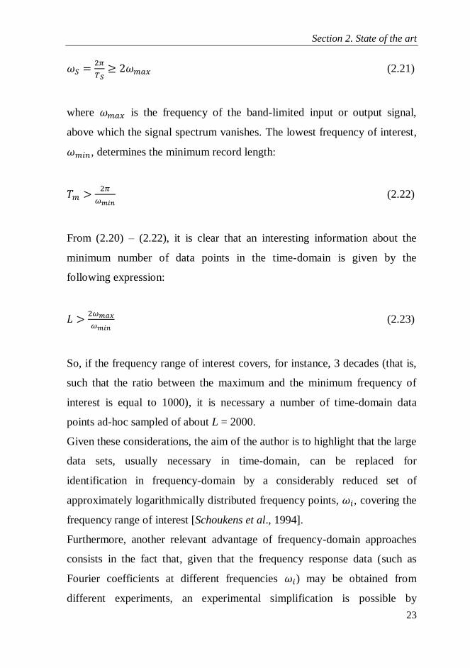
(2.21)
where is the frequency of the band-limited input or output signal,
above which the signal spectrum vanishes. The lowest frequency of interest,
, determines the minimum record length:
(2.22)
From (2.20) – (2.22), it is clear that an interesting information about the
minimum number of data points in the time-domain is given by the
following expression:
(2.23)
So, if the frequency range of interest covers, for instance, 3 decades (that is,
such that the ratio between the maximum and the minimum frequency of
interest is equal to 1000), it is necessary a number of time-domain data
points ad-hoc sampled of about L = 2000.
Given these considerations, the aim of the author is to highlight that the large
data sets, usually necessary in time-domain, can be replaced for
identification in frequency-domain by a considerably reduced set of
approximately logarithmically distributed frequency points, , covering the
frequency range of interest [Schoukens et al., 1994].
Furthermore, another relevant advantage of frequency-domain approaches
consists in the fact that, given that the frequency response data (such as
Fourier coefficients at different frequencies ) may be obtained from
different experiments, an experimental simplification is possible by

Section 2. State of the art
24
combining data from different experiments, which is not so easily possible in
time-domain identification procedures.
Finally, it is worth highlighting that all the symbols adopted in Section 2 are
those usually adopted in the technical literature in the specific field of
system identification. This is due to a specific author‟s decision, who
preferred to avoid confusion in interested readers, who could refer to the
numerous papers cited in the present section in order to acquire more
detailed information on the identification of CT linear systems. For the same
reason, some of the symbols adopted in Section 2 will be provided also in
following sections but with a completely different meaning, in order to
assure a continuity with the existing literature works concerning the study of
stochastic shot noise modeling of daily streamflows.
Section 3. Calibration of shot noise process-based models
25
3. Calibration of shot noise process-based
models
3.1. Introduction
In Section 2 the more frequently adopted identification techniques of CT and
TI models, both in the time-domain and in the frequency-domain, have been
reported. Nevertheless, the main subject developed in this Ph.D. dissertation
deals with a spectral domain-based identification approach of a particular
class of models for daily streamflows reproduction and generation, known as
shot noise process based-models (for the sake of brevity, from this moment
the author will refer to this class of models as shot noise models).
In the present section, a brief description of the scientific background
concerning those models intended to the reproduction, forecasting and
simulation of short-time discharge data will be firstly provided. At a later
stage, general time and spectral-domain properties of the shot noise process
will be described, and, eventually, a comprehensive description of shot noise
models identification techniques will be provided.

Section 3. Calibration of shot noise process-based models
26
3.2. Reproduction of short time scale discharge series: a survey
Nowadays it is well recognized the difficulty in the use of limited
streamflow time series in water resources planning and management
problems. As a consequence, during the last decades, stochastic streamflow
simulation has been attracting great interest among the scientific community,
in particular thanks to its utility in optimization techniques [e.g., Karamouz
and Houck, 1987; Karamouz et al., 1992; Chang and Chang, 2001; Ahmed
and Sarma, 2005]. As a matter of fact, these methods produce synthetic
streamflow traces that reflect the statistical properties of the historic data.
Depending on the particular problem, the reproduction of the streamflow
process is desired at different time resolution. In the past forty years, several
classes of stochastic models were proposed, which generally looked at each
time scale of aggregation individually. But in order to deal with water
resources planning and management problems on a daily scale, the
reproduction of short-time (that is, from daily to weekly) discharge data is
needed. In particular, short time streamflow series are characterized by the
presence of the intermittent pattern of dry/wet periods and by the skewed
nature of the hydrographs, with sudden discharge increases and slow
recessions [Murrone et al., 1997]. These features prevent the use of
parametric and non-parametric methods (e.g., Auto Regressive Moving
Average K-Nearest Neighbor, etc.) [see, e.g., Lall and Sharma, 1996;
Ouarda et al., 1997; Prairie et al., 2006], which, instead, are successfully
applied to monthly and annual data.
The aptitude to reproduce the presence of peaks and recessions in daily
discharge time series belongs to the filtered point processes [Bernier, 1970],
also known as Shot Noise (SN) processes, that have received considerable
attention in hydrologic literature [Weiss, 1977; Koch, 1985; Xu et al., 2002].

Section 3. Calibration of shot noise process-based models
27
The structure of this process consists of a point process that reproduces the
occurrence (that is the sequence of effective rainfall events) which acts as
the input of a system that is representative of the watershed transformations.
Runoff is obtained by filtering the input through the system response
function.
The first comprehensive work on SN models of runoff was due to Weiss
[1973; 1977], who introduced a model in which effective rainfall events
were reproduced through a Poisson process of occurrences coupled to
exponentially-distributed intensities. A two-component SN process results
from this scheme, and the method of moments was proposed for parameter
estimation. A more recent improved variant of Weiss‟ model was instead
due to Cowpertwait and O'ConnelI [1992], who proposed the Neyman-Scott
model to reproduce the effective rainfall process. Between Weiss [1973] and
Cowpertwait and O'ConnelI [1992], several approaches, often based on SN
formulation, were proposed for short-time runoff modeling (please refer to
Murrone et al. [1997] for a comprehensive literature review). In particular,
among them, it is worth underlining the contribution of Treiber and Plate
[1977], Yakowitz [1979], Pegram [1980], Hino and Hasebe [1981],
Vandewiele and Dom [1989], who proposed different linear or non-linear
conceptual scheme of the watershed based on a SN formulation.
A central point in the use of SN process-based methods is the calibration
procedure adopted for the evaluation of the parameters on which the selected
form of the system response function is based. In particular, most of the
existing, and most recent, literature works are based on a time-domain
iterative identification approach that consists of the minimization of the
squared differences between the observed discharge values and those
obtained by the convolution of the response function (to be identified) and

Section 3. Calibration of shot noise process-based models
28
the input series [Murrone et al., 1997; Claps and Laio, 2003; Claps et al.,
2005; Xu et al., 2001].
A crucial aspect in the application of a time-domain approach concerns the
generation of the occurrences (or effective rainfall) to be convolved with the
watershed response function of a given form but with unknown parameters.
As a matter of fact, the model parameters estimation is deeply dependent on
the method chosen for the effective rainfalls modeling. For this reason,
hereinafter, the authors will provide a thorough description of the main
approaches available in the scientific literature for the effective rainfall
occurrences and intensities determination.
3.3. Shot noise models: main statistical properties
Given a set of Poisson distributed points (i.e. the time of occurrence of the
ith input pulse) with average density , the following process is given:
∑ (3.1)
where is the time variable, is a sequence of independent and identically
distributed (i.i.d.) random variables, independent of the points (i.e. the
instant values corresponding to the effective rainfall occurrences), with mean
and variance [Papoulis and Pillai, 2002, Subsection 10.2]. Hence the
process is a staircase function with jumps at points , equal to . The
process is the number of Poisson points in the interval , hence its
expected value is { } and its second order moment is { }
. From this, it follows that:
{ } { } (3.2)

Section 3. Calibration of shot noise process-based models
29
{ } { }
{ }
(3.3)
It could be now possible to demonstrate that (but it is here avoided for the
sake of conciseness):
(3.4)
where is the autocovariance function of the process .
The next step is to consider the impulse train, given by the following
expression, which determines the so called Shot Noise (SN) process and that
can be adopted to model the entire rainfall process:
∑ (3.5)
where is the Dirac delta function.
Given Eq. (3.4), it follows that:
{ }
{ } (3.6)
(3.7)
Convolving the SN process, i.e. the impulse train (3.5), with a function
(that, in the hydrologic application, is representative of the watershed
response function) the Generalized Shot Noise (GSN) process is obtained:
∑ (3.8)

Section 3. Calibration of shot noise process-based models
30
where is the streamflow variable, intended as a continuous time
variable. Its main statistical properties are provided by the following
expressions:
{ } { } ∫
(3.9)
(3.10)
{ }
∫
(3.11)
where { } is the streamflow variable variance.
Given the general formulation of SN processes, the intention of the author is
now to highlight some of their properties that are necessary for the
comprehension and the application of the frequency domain identification
procedure proposed in this thesis.
In particular, as revealed by Eq. (3.7), it is fundamental to underline the
impulsive nature of the input process autocovariance function .
While the commonly adopted time-domain identification approaches, that
will be discussed in Subsection 3.4, do not take any advantage from this
powerful property, it is the basic principle on which the spectral-domain
identification procedure here proposed was built. In particular, it is well
known that the power spectrum , or, more concisely, the spectrum, of a
real or complex process is the Fourier transform of its autocovariance
function . Hence the following relation is valid:
∫
(3.12)

Section 3. Calibration of shot noise process-based models
31
where is the imaginary unit and is the angular frequency. Similarly, it is
worth underlining that the well-known Power Spectral Density (PSD) of the
generic process , or, more simply, its spectral density, is defined as the
Fourier transform of the autocorrelation function of the process itself,
suggesting that it is obtainable dividing the spectrum (3.12) by the variance
of the process [Jenkins and Watts, 1968, p. 218]. This is the reason why it is
not rare, in a system identification environment, to talk about the PSD
instead of the spectrum of a given process. Thus, for the sake of simplicity,
hereinafter the author will refer to the functions defined as in the equation
(3.12) as PSDs.
Given the above considerations and starting from Eq. (3.7), which shows the
autocovariance expression of the impulse train process , it should be
evident that the PSD of is equal to a constant, as provided by the
following equation:
(3.13)
Thus, considering that in case of linear systems the following relation is
valid [Papoulis and Pillai, 2002, p. 412]:
| | (3.14)
where and are, respectively, the PSDs of the system response, ,
and of the input process, , H(ω) is the linear system TF and H*(ω) its
complex conjugate, it is clear that, given the Eq. (3.13) and the superposition
effect valid for linear systems, in case of SN model the following equation
holds:

Section 3. Calibration of shot noise process-based models
32
| | [
]| | | | (3.15)
From Eq. (3.15) it is evident how the contribution of the impulse train
spectral density, , is only that of a scale factor, , between the spectral
density of the system response, , and the linear system TF, . Hence,
starting from the knowledge of the output process, i.e. when river flow data
are available, one can estimate the parameters of the watershed response
function (model calibration) only by matching the PSD amplitudes,
estimated at several frequencies, of the observed river flow records with the
squared module of the linear system TF.
However, it is worth noticing that, as outlined by Montanari and Toth
[2007], the PSD of a process does not convey any information about the
mean of the process itself. As a consequence, in this work, in order to allow
the correct reproduction of the recorded streamflow series mean
characteristics, obviously affected by seasonality, the author decided to
include all the information on the mean of the output process, in the
input process, , also known as effective rainfall process [see, for
reference, Murrone et al., 1997]. Hence, the TF parameters estimation was
undertaken, following the aforementioned Eq. (3.15), on the PSD, , of the
deseasonalized streamflow process, , in order to avoid that the
seasonality of the streamflow process mean level affected the form of the
PSD and, thus, the estimated values of the parameters. More details about
the deseasonalization processes are provided in following sections.
As outlined in following Subsection 3.5, the main advantage of the proposed
spectral-domain calibration procedure consists in the possibility to estimate
the values of the TF parameters independently from the knowledge of input
process data information, provided that, in the case of SN assumption, the
PSD of the input process contributes to each frequency value with the same

Section 3. Calibration of shot noise process-based models
33
amplitude. As a consequence, the procedure here presented is particularly
suitable for the resolution of model calibration problems in the case of
ungauged basins [see, for reference, Montanari and Toth, 2007] (i.e., those
watersheds that are not provided with systems aimed at the recording of
hydro-meteorological processes), which is a really common situation in
developing countries where the demand of simulation tools, for design and
management of new hydro-power systems, is increasing.
Moreover, thanks to this remarkable characteristic of the calibration
approach, the whole proposed methodology differentiates itself from the
limited number of other frequency-domain approaches, for the calibration of
SN models, available in the scientific literature. A relevant contribution to
this topic was that by Diskin and Pegram [1987], who dealt with the
spectral-domain calibration of a cell model for storm-runoff modeling, with
available records of a particular storm and flood hydrograph event. In
particular, the whole calibration procedure, once defined a model made by a
proper combination of linear reservoirs, was based on the minimization of an
objective function given by the sum of the differences between the Laplace
transforms (estimated at several frequency values) of the recorded output
sequence and that of the model output. The overall approach, however, was
based on the analytical knowledge of Laplace transforms of the output and
input signal (other than that of the basin response function), starting from the
knowledge of the structures of input and output sequences (i.e., respectively,
a histogram structure and a polygon structure). It is thus clear the advance
that the calibration approach here described introduces, in the scientific
literature, in the field of spectral identification approaches of shot noise-
based models.

Section 3. Calibration of shot noise process-based models
34
In order to complete the position of SN process, some other few properties
need to be provided. Since the density of the Poisson points and the
distribution of the amplitudes are assumed independent of time, the SN
process results stationary, with a mean, as shown in Papoulis and Pillai
[2002, p. 461], reported in the following equation:
[ ] (3.16)
The non-stationarity of the SN, that is useful for example to model
seasonality, may arise from two different sources:
(a) the dependence of on time;
(b) the dependence of distribution on time.
However, in both cases, following Roberts [1965], a useful equation that
relates the mean of the streamflow process to properties of the rainfall
process can be established as follows:
[ ] [ ] (3.17)
In Eq. (3.17), is the time-varying density of the Poisson points and
is the time varying (conditional) expected value of the pulse amplitude,
given that there is a pulse in the interval [ ]
Starting from the assumptions and the considerations about the SN process
presented in the present section, in Subsection 3.4 the author will firstly
provide a detailed description of the most adopted calibration approaches, in
the scientific literature, of SN-based hydrological models. At a later stage,
moreover, the effectiveness of spectral calibration methods will be shown,
assuming stationarity of the SN process, thus leaving to future works the
exploitation of non-stationarity.

Section 3. Calibration of shot noise process-based models
35
3.4. Shot noise models: classical calibration approaches
The procedure for parameters estimation of SN models is strictly related to
the approach followed for the parameters estimation of the model of
effective rainfall. In particular, for this latter goal, two alternatives are
essentially available in the technical literature.
In the first one, common to most of the SN models in literature [see, for
reference, Weiss, 1973, 1977; O'Connell and Jones, 1979; Cowpertwait and
O'Connell, 1992], the form of the underlying input process is pre-determined
and its parameters are estimated through the method of moments applied to
the streamflow statistics [Murrone et al., 1997]. The main drawback of this
procedure are:
(a) the fact that it does not allow the users to verify the hypothesis made on
the input process;
(b) the impossibility to evaluate the influence of the effects of the watershed
transformations on the estimation of the effective rainfall model parameters.
In the alternative approach these problems are overcome since the input
series is reconstructed by inverse estimation. On the obtained series,
parameters of the stochastic input model are thus evaluated. Several authors
followed this latter procedure, each with a different ad-hoc introduced
technique [see, among others, Treiber and Plate, 1977; Hino and Hasebe,
1981, 1984; Battaglia, 1986; Wang and Vandewiele, 1994].
Concerning this latter procedure, a relevant scientific contribution was that
of Murrone et al. [1997]. In this paper, the authors firstly defined the form of
the basin response function . In particular, it was assumed linear and
given by the linear combination, through coefficients , of the individual
responses of its components. Each component was modelled as a linear

Section 3. Calibration of shot noise process-based models
36
reservoir, with a corresponding Instantaneous Unitary Hydrograph (IUH) of
exponential negative form. In order to test the procedure in various case
studies, the authors decided for a basin response function given by the
combination of 3 linear reservoirs (each representing one among the sub-
daily, over-month and over-year groundwater contributions). Moreover, the
response function contribution corresponding to the surface component was
modelled as an additional Dirac delta function, since the basin surface
response lag was enough smaller than the time interval of data aggregation
(considered from daily to weekly).
Starting from these considerations, the estimation of the model parameters
(i.e. linear combination coefficients, , and storage coefficients, , for each
of watershed contribution) was undertaken, through minimization of the
squared differences between recorded flow values and those obtained
through convolution of the effective occurrences and the basin function. For
this purpose, an iterative procedure resulted necessary, since the input
intensities (hereafter defined as effective rainfall), in turn, were obtained by
deconvolution of the recorded streamflow series through the system response
function with unknown parameters.
Finally, for the generation of synthetic streamflow series, fundamental for
the statistical verifications, a Poisson White Noise Exponential Model
(PWNE) [Eagleson, 1978] was fitted on the final effective rainfall series. In
this manner, the generation of synthetic effective rainfall series, to convolve
with the identified response function, was allowed.
It is worth noticing the approach followed by the authors in the selection of
rainfall occurrences and intensities at the first iteration, that is when no
estimates of the response function parameters are available. Indeed, the net
rainfall occurrence was assumed in each time instant presenting a discharge
increase. However, in order to account for errors in discharge measurements,

Section 3. Calibration of shot noise process-based models
37
a threshold value, , was considered. In particular, only when the
condition was met, a trial value of the rainfall amount was
assumed equal to [Battaglia, 1986]. The choice of the
threshold level was thus critical because of its direct influence on the number
of input events.
The main drawback in the adoption of such a procedure dealt with the
necessity of several iterations to obtain the final parameters estimation,
resulting in a lack of robustness of the overall approach. Moreover, few
details were given by Murrone et al. [1997] about the selection of the
threshold, , value in the estimation of effective rainfall occurrences and
intensities at the very first iteration. For the sake of conciseness, from this
moment the author will refer to this method, for the selection of effective
rainfalls, as Discharge Increments Pulses (DIP) approach [see Claps and
Laio, 2003]. Even though frequently adopted, the DIP approach presented
two relevant drawbacks [Claps et al., 2005]. First of all, the presence of
noise in the daily streamflow measurements could result in small rises in the
flow process records, resulting, in turn, in an overestimation of the mean
number of rainfall events per year. Secondly, the basic hypotheses of
mutually independent and Poisson-distributed pulses were often not
respected by the estimated sequences.
In order to overcome these two main drawbacks, Claps and Laio [2003]
presented an evolution of the DIP approach. The Filtered Peak Over
Threshold (FPOT) method was introduced in order to derive a more
appropriate pulse sequence. Its main steps can be summarized as follows:
(a) given the recorded daily discharge series, the occurrences are found in
correspondence of all the local maxima of the series itself;
Section 3. Calibration of shot noise process-based models
38
(b) given the local maxima values, a sequence of Filtered Peaks (FP) is
determined by subtracting the first local minimum preceding the considered
peak;
(c) a threshold filter is increasingly applied to the FP series, in order to retain
only significant peaks, until the peaks independence test of Kendall and the
peaks Poisson distribution test of Cunnane are jointly met.
As stated by the authors themselves, the adoption of the FPOT approach
guarantees the following advantages if compared to the DIP one:
(1) it allows one to avoid the deconvolution step in the peaks identification
procedure, with considerable advantages in terms of procedure simplicity
and robustness;
(2) it returns an effective rainfall series that automatically meets both the
independence and Poissonianity requirements of the PWNE model.
Nevertheless, they also noticed that, as major drawback, the number of
selected peaks is reduced to 5-20 per year [Claps et al., 2005], which
underestimates the actual number of effective rainfall events. Such a
consideration would suggest the inadequacy of the Poisson independent
model in the correct reproduction of the effective rainfall behaviour.
Another notable contribution to the identification of SN models was that of
Xu et al. [2001; 2002], in which the daily streamflow process was regarded
as a sum of two components with different characteristics, i.e. the direct
surface runoff and the baseflow. In particular, the former, responsible of the
short-term variations, was considered as an intermittent process with a
Gamma response function. The latter was instead characterized by the
conventional negative exponential response function (that of subsurface and
groundwater storages) and was considered responsible for the long-term
persistence displayed by the recorded streamflow series. Both the

Section 3. Calibration of shot noise process-based models
39
components to the total streamflow process were calibrated by means of
physical considerations on the case study watershed considered in the
application, that are not reported here because not relevant according to the
main goal of the present thesis.
However, the notable contribution of the authors consisted in the procedure
introduced for the estimation of pulse intensities necessary in the synthetic
streamflows generation. Indeed, as in the previously described works, they
referred to a sequence of uncorrelated rainfall pulses but following a Gamma
probability distribution. In order to estimate the distribution parameters,
starting from the recorded streamflow series, the authors followed these two
steps:
(a) to determine the occurrences, they assumed that pulses occur only on
those days when streamflow increases;
(b) to estimate pulses intensity, they made a least-squares fit of the
reconstructed streamflow series (obtained through convolution of the input
sequence with the known time response function) and the recorded one,
assuming, of course, the unknown input intensities as the variable to be
determined. Subsequently, in order to test the assumption of storm events
compatible with a non-homogeneous Poisson point process (i.e. defining a
different Poisson process, of a given parameter, for each month), the
goodness-of-fit test was made for each month.
Although the calibration approach presented in this work, that takes
advantage of the SN model spectral properties described in Subsection 3.3, is
completely independent from the technique adopted in the parameters
estimation of the model of effective rainfall, it is of considerable interest due
to its importance in the synthetic streamflow generation. As a matter of fact,
a simulation analysis is necessary to assess the effectiveness of the model in

Section 3. Calibration of shot noise process-based models
40
the reproduction of the main statistical features of the recorded series. For
this purpose, in this thesis the author has selected the latter approach
described, i.e. Xu et al. [2001; 2002], given its better performances, in terms
of effective rainfalls features reproduction, verified in the following
subsections.
3.5. A spectral domain calibration procedure
3.5.1. Model structure: the watershed response function
Given the aforementioned modification of Eq. (3.15), in which, for each
angular frequency , the PSD of the deseasonalized streamflow process
( ) is equal to the squared module of the watershed TF ( ), in
order to allow its application to a general case study, the definition of the
shape of the basin response function is needed. For this purpose, a
preliminary description of how effective rainfall reaches the basin outlet is
needed. In particular, three main runoff components can be identified: the
baseflow (i.e. the return flow from groundwater capacities), the subsurface
flow (i.e. interflow, representing rapid flow through pipes, macro-pores and
seepage zones in the soil) and saturated overland flow (surface flow). The
two latter components form the direct runoff, also known as quickflow. It is
worth underlying that separation of effective rainfall into the above
components is non-linear, because the relative weight between direct and
groundwater runoff depends on the infiltration capacity, that is function of
the soil moisture state and of the intensity of rainfall. Nevertheless, this non-
linearity is not considered here, essentially because it is thought that for the
aims of the analysis undertaken it is more important to test how well the

Section 3. Calibration of shot noise process-based models
41
proposed framework is able to reproduce main runoff process features at
different frequencies.
Regarding the baseflow, Claps et al. [1993] demonstrated that, even in small
basins, annual data can be autocorrelated, due to the presence of a
groundwater contribution with very slow response time. Hence, even though
in large basins the hydrogeologic scheme could be more complex, it is
convenient to assume that when an annual autocorrelation is present in the
considered time series this is due to the presence of a large and deep aquifer.
Moreover, those authors also showed that in monthly data autocorrelation is
present even when annual runoff is uncorrelated. As a consequence, the
presence of a groundwater component that introduces “memory” in runoff
data with a delay time of the order of few months is revealed. This over-
month groundwater component is due to the presence of aquifers which run
dry within the dry season.
Eventually, as regards direct runoff, if the basin is sufficiently large, even on
daily data one can recognize the presence of both the subsurface and the
surface runoff components.
Therefore, from these considerations it follows that one cannot exclude that
all four of the above components can be identified from the streamflow
dynamics on a short time scale. Consequently, the most general watershed
scheme includes four conceptual elements in parallel.
Starting from the above considerations, in order to undertake, in the
following subsections, some comparisons with results obtained by well-
known literature works, in this thesis the author has referred to the same
response function shape adopted by Murrone et al. [1997]. In this latter work
a conceptual model of the watershed is considered, with a basin response
function given by the linear combination, through coefficients , of its
components contributions. Each component, modelled as a linear reservoir

Section 3. Calibration of shot noise process-based models
42
(hence with a negative exponential impulse response given in Eq.
(3.18)), is representative of a corresponding groundwater contribution to the
streamflow process, each with a proper storage coefficient :
⁄⁄ (3.18)
The component identified by the coefficient (see Eq. (3.19)) is instead
representative of that amount of effective rainfall that reaches directly the
basin outlet (surface runoff), i.e. with a response time enough smaller
than the interval of data aggregation and, for this reason, modeled as a Dirac
delta function [Claps et al., 2005]. Thus, it is possible to assume the
following form of the time response function:
⁄
⁄
⁄ (3.19)
In the previous equation the groundwater components represented by the
storage coefficients are: the sub-daily ( , representing the sub-surface
runoff); the over-month ( , representing the contribution of those
groundwater capacities that are dry during the dry season); the over-year ( ,
representing deepest aquifers). Moreover, it is worth underlying that
coefficients , which are considered constant and which distribute the input
volume among system elements, according to the continuity condition, have
to fulfil the continuity condition: ∑ .
Given the response function shape of Eq. (3.19), in order to apply the
spectral property of Eq. (3.15), the analytical determination of the
corresponding TF form ( ) is needed. Starting from the well-known

Section 3. Calibration of shot noise process-based models
43
properties of the Laplace transform, which are not reported here for the sake
of conciseness, it is possible to demonstrate that the Laplace transform,
, of the system response function of Eq. (3.19) is given by the following
expression:
{ }
(3.20)
where s is the complex Laplace variable ( ), given by the
summation of its real ( ) and imaginary ( ) parts.
Assumed the result shown in Eq. (3.20), it is now fundamental to determine
the TF module. In particular, in order to make it estimable at discrete
frequency values, it is needed to pass from the Laplace ( ) to the Fourier
( ) domain, given that the latter is the restriction of the former to its
imaginary axis (i.e., assuming that in Eq. (3.20)). Starting from this
premise, once obtained the TF real ( ) and imaginary ( ) parts, that are
not analytically reported here for the sake of brevity, the TF magnitude is
easily obtainable, by the definition of the module of a complex number, as
| | √ , which leads to the following expression:
| | [(
)
(
)
]
(3.21)
with f the frequency value, expressed in Hertz, at which the module of the
TF is estimated (which is related to the angular frequency by the following
well-known relation: ⁄ ).

Section 3. Calibration of shot noise process-based models
44
In Section 4 it will be shown that, once numerically estimated the PSD of the
streamflow process at discrete frequency values ( ), the TF module of Eq.
(3.21) will be directly adopted in the estimation of the unknown watershed
parameters.
A crucial aspect that needs to be underlined consists in the fact that, thanks
to the shape of the watershed response function adopted in this thesis, the
basin response function is that of a minimum phase system. In the scientific
literature a minimum phase system is that corresponding to a TF with two
particular features: (a) a positive gain; (b) all poles and zeros with a
negative/null real part [Bolzern et al., 2004]. For this reason, in such a
system an unique relation between the amplitude and the phase diagrams of
the systems response exists. It is thus possible to neglect the phase of the
streamflow signal and calibrate the watershed response function only by
fitting its PSD.
According to the work of Muratori et al. [1992], about the minimum phase
property of single-input single-output linear compartmental systems (i.e.
networks of linear reservoirs), both the connection of n linear reservoirs in
cascade and in parallel have minimum phase characteristics (see theorems 1
and 2 of the cited work). Therefore, given the form of the response function
shown in Eq. (3.19), corresponding to the parallel connection of four linear
reservoirs (with the one corresponding to the surface runoff characterized by
a detention time enough smaller, and thus negligible, if compared to the
data aggregation scale), it is possible to state that the system considered in
this work possesses minimum phase properties. However, it is worth
underlying that, given the minimum phase conditions reported in the cited
work, several conceptual models based on the parallel and cascade
connection of linear reservoirs, frequently adopted in hydrologic calibration

Section 3. Calibration of shot noise process-based models
45
problems, have minimum phase properties. Hence, once clarified the
minimum phase property associated to the adopted response function of Eq.
(3.19), it is possible to state that, according to Eq. (3.15), in the present
thesis the watershed model has been calibrated only by numerically
matching, at each frequency, the squared values of Eq. (3.21) to the
transformed streamflow process PSD, without paying any attention to the
phase signal information.
It is worth noticing that, as stated by Nikias and Mendel [1993], the
autocorrelation, or equivalently the spectral density, domain suppresses all
phase information about the system to be identified. As a consequence, a
proper system calibration by the adoption of procedures based on the use of
only PSD functions is possible only if the system is minimum phase, that is
only if an univocal relation between magnitude and phase features of the
model exists. As a matter of fact, the adoption of PSD-based techniques
allows only the identification of minimum phase systems [Nikias and
Mendel, 1993].
3.5.2. PSD estimation techniques
3.5.2.1. A brief overview
Given the result shown in Eq. (3.15) and the expression of the TF module
showed in Eq. (3.21), in the present subsection the author will provide an
overview about PSDs, or equivalently power spectra, estimation techniques.
The techniques for estimating the conventional power spectrum fall into two
main categories:
(a) the nonparametric or conventional methods;
(b) the parametric or model-based methods;
Section 3. Calibration of shot noise process-based models
46
The first category, in turn, includes two classes: the direct methods, which
are based on the FT of the observed data, and the indirect methods, which
consist in the computation of the FT of the estimated autocorrelation
sequence of the data (e.g., the periodogram technique). The second class,
that of parametric methods, includes algorithms such as MA, AR, and
ARMA modeling, and eigen-space based methods such as MUSIC, Min-
Norm, etc., which are appropriate for harmonic models. Hereinafter the main
features of the aforementioned categories of methods are described, with a
particular focus on the adoption of the periodogram (widely adopted in
technical literature) and of the autoregressive (AR) method, also known as
maximum entropy method (MEM).
3.5.2.2. Nonparametric (or conventional) methods
The conventional estimators (or nonparametric ones) are generally easy to
understand and easy to implement, but they are limited by their resolving
power (the ability to separate two closely spaced harmonics), particularly
when the number of samples is small. For random signals, these estimators
typically require long observation intervals in order to achieve acceptably
low values for the variances of the estimate.
The most adopted nonparametric estimator of the power spectrum of
a generic time signal , about which recorded sampled values are
available, is certainly the so-called periodogram [see, e.g., Montanari and
Toth, 2007], defined as the discrete FT of the autocovariance function
:
∑
|∑
| (3.22)

Section 3. Calibration of shot noise process-based models
47
As clearly showed, the periodogram can also be estimated as the squared
value of the absolute value of the discrete FT of the time signal . It is
worth noticing that the periodogram is an unbiased estimator of the
spectrum, even though its variance at any frequencies does not go to zero as
the number of samples goes to infinity (i.e. it is not a consistent estimator).
Nevertheless, as increases the spacing between estimates that are
uncorrelated decreases as , thus the fluctuations in the periodogram
become more rapid. However, there are several ways to make consistent the
periodogram estimation, among which it is possible to distinguish between:
- smoothing (or filtering) in the frequency domain (that leads to the well-
known Blackman-Tukey spectral estimator, which can be considered as a
“locally” weighted average of the periodogram [see, for reference, Stoica
and Moses, 2005, Subsection 2.5]);
- averaging several periodogram estimates (Barlett, Welch and Daniell
methods [Stoica and Moses, 2005, Subsection 2.7]).
For the sake of conciseness the author will not provide any description of the
aforementioned techniques, thus the interested reader is referred to the
numerous technical works concerning this matter (among which Stoica and
Moses [2005] Section 2 is suggested).
3.5.2.3. Parametric (or model-based) methods
The second category is that of parametric methods, which are based on
parametric models of a time series, such as autoregressive (AR) models,
moving average (MA) models, and autoregressive-moving average (ARMA)
models (this is the reason why they are also known as model-based
methods). To estimate the spectrum of a time series with parametric

Section 3. Calibration of shot noise process-based models
48
methods, thus, you need to firstly select an appropriate model and, secondly,
obtain the model parameters of the time series.
The AR or all–pole signals constitute the type that is most frequently used in
applications. The AR equation may model spectra with narrow peaks, that is
an important feature since narrowband spectra are quite common in practice.
The estimations of AR model parameters are usually found by solving a
system of linear equations, and the stability of the estimated AR polynomial
can be guaranteed. In general, two techniques are considered for the
estimation of AR parameters. The Yule Walker method that is base directly
on the linear relationship between the covariances and the AR parameters.
The Least-Square (LS) method, based on a LS solution of AR parameter
from the corresponding time-domain equation [Stoica and Moses, 2005,
Subsection 3.4].
The MA signal is obtained by filtering white noise with an all–zero filter.
Owing to this all–zero structure, it is not possible to use an MA equation to
model a spectrum with sharp peaks unless the MA order is chosen
“sufficiently large”. Thus this contrasts with the ability of AR model to
model narrowband spectra by the adoption of low model orders. On the
contrary, the MA models allow the fitting of spectra with broad peaks and
sharp nulls. Such spectra are not really spread in engineering applications,
thus limiting the adoption of MA models in the estimation of PSD functions.
Moreover, MA parameter estimation problem is basically a nonlinear one,
thus the type of difficulties one should face in MA and more complete
ARMA estimation problems are quite similar, so one usually prefers the use
of the latter typology [Stoica and Moses, 2005, Subsection 3.5].
For spectra with both sharp peaks and deep nulls a modeling by either AR or
MA equations of reasonably small orders is not reasonable. In these cases
the adoption of the more general ARMA model, also called the pole-zero

Section 3. Calibration of shot noise process-based models
49
model, is suggested. Two main groups of estimators of ARMA models are
available in the technical literature. The “theoretically optimal” estimators
are based on iterative procedures whose global convergence is not
guaranteed. The “practical estimators”, on the other hand, are
computationally simple and often quite reliable, but their statistical accuracy
may be poor in some cases. The mainly adopted techniques in the estimation
of ARMA type spectra are the so called Modified Yule-Walker method and
the Two-Stage least square method. However, the intention of the author is
not that of focusing on this typology of spectrum estimator, thus the
interested reader is referred to Stoica and Moses [2005, Subsection 3.7] for
more details.
Given the classical features of common power spectra in hydrologic
applications, the author has opted in favour of the AR typology among
parametric estimators. Hence, hereinafter, a more detailed description of the
all-poles model is provided.
First of all, consider the transformation of the complex f-plane to a new
plane, called the z-plane, through the relation:
(3.23)
where Δ is the sampling interval of the continuous signal in the time domain
(it is worth noticing that, limited to the present subsection, the reader must
not confuse the variable above defined with the one representing the
impulse train process in the described shot noise structure).
A formal expression to represent the “true” spectrum is the following
Laurent series that depends on the infinite number of values :

Section 3. Calibration of shot noise process-based models
50
|∑
| (3.24)
The (3.24) can be intuitively approximated in a general manner with a
rational function with two finite series in both the numerator and the
denominator. Less obviously, instead, there are some advantages in an
approximation whose free parameters all lie in the denominator (all-poles
approximation):
| ∑
| (3.25)
As mentioned above, the approximation (3.25) of the real power spectrum
goes under different names: indeed, apart from all-poles (where is the
number of poles adopted for the estimation) or autoregressive model, it is
also usual to refer to Eq. (3.25) as maximum entropy method (MEM)
approximation. Coefficients can be evaluated by means of several
estimation methods, among which the author has selected the Burg
algorithm, developed by Burg [1975] and based on forward and backward
prediction errors (see, for reference, Stoica and Moses [2005] Subsection
3.9.3).
Two main consideration need to be made concerning the all-poles spectra
estimation technique.
Firstly, the author wants to justify the reason behind the name MEM of the
method. As underlined by Press et al. [1996, Subsection 13.7], whatever is
the chosen value of in (3.25), the series expansion in the equation defines
a sort of extrapolation of the autocorrelation function to lags larger than ,
even to lags larger than the number of measurable data . It results this
particular extrapolation can be shown to have, among all possible

Section 3. Calibration of shot noise process-based models
51
extrapolations, the maximum entropy in a definable information-theoretic
sense. Because of this “fictitious” property, it is thought in general that it
gives intrinsically better estimates if compared to other methods. Obviously,
after this short explanation, one will be sure that this common assumption is
totally unfounded.
The second consideration deals with the number of poles (or order of the
AR method) to adopt in the expansion series of Eq. (3.25). As reported by
Press et al. [1996, Subsection 13.7], in common applications it is used to
limit the order of the MEM approximation to a few times the number of
sharp spectral features that are desired to be fitted. In this way, the method
tends to smooth the spectrum, that is often a desirable property to achieve. In
general, however, even though exact values depend on the application
considered, one might take equal to 10 or 20 or 50 for equal to 1000 or
10000, in order to make the MEM estimation not much slower than the Fast
Fourier Transform (FFT) estimation.
3.5.3. The calibration approach
3.5.3.1. The parameters estimation
Once defined a form for the watershed TF, whose absolute value is showed
in Eq. (3.21), in order to best model the behaviour of the basin forced by the
effective rainfall process, the estimation of the unknown parameters vector θ
is possible by the adoption of Eq. (3.15). For this aim, the estimation of the
deseasonalized streamflow process PSD ( ), by the use of the
aforementioned MEM method, was accomplished. Conversely, no
estimation of the input process PSD was necessary ( ) since, as shown in

Section 3. Calibration of shot noise process-based models
52
Eq. (3.15), its contribution in the relation between the output process PSD
and the squared module of the TF is only that of a constant ( ).
As widely repeated in previous sections, in order to allow the adoption of
Eq. (3.15), it was necessary to deseasonalize the recorded streamflow series,
. For this purpose, even though not reported here for the sake of
conciseness, the deseasonalization method, clearly described in Hipel and
McLeod [1994, Chapter 13], consisting in the difference between the generic
series value with the mean of its corresponding season, was adopted.
Starting from these premises, the parameters estimation was conducted in a
least square (LS) framework. The minimization of the sum of the squared
differences between the numerical estimation of the deseasonalized
streamflow process PSD, normalized in the range 0-1 ( ), and the analytic
expression of the squared module of the TF (3.21), estimated in the
frequency range of interest [ ], was thus undertaken (refer to the
following equation):
∑ [ | | ]
(3.26)
Concerning the applied procedure, some important aspects need to be
discussed.
First of all, it is worth noticing that the contribution of the constant PSD
value (G) of the input process was neglected in the determination of the TF
parameters. This was mainly due to the fact that, in order to minimize the
function of Eq. (3.26), its value must equal the value assumed by the
PSD at the lowest frequency of the frequency range of interest (the so called
static gain). This is the reason why the model calibration was performed
considering the PSD normalized in the range 0-1 ( ), obtained by

Section 3. Calibration of shot noise process-based models
53
dividing each amplitude value by that assumed in correspondence of the
lowest frequency.
Secondly, as above stated, a frequency range of interest [ ] was
defined in the minimization of Eq. (3.26). In order to understand such a
decision of the author, consider Eq. (3.12) that defines the power spectrum
( ) as the FT of the autocovariance function ( ) of the generic time
signal . As a matter of fact, the following inverse transform holds:
∫
(3.27)
from which it follows, setting the lag :
∫
(3.28)
Eq. (3.28) demonstrates that the power spectrum shows how the variance (or
mean power) of the time process is distributed over frequency [Jenkins and
Watts, 1968, chapter 6.2]. Specifically, the variance of the process which is
due to frequencies in the range - is approximately . It is
thus clear that by integrating the power spectrum in a certain frequency
range gives the amount of the total variance (or mean power) in that range.

Section 3. Calibration of shot noise process-based models
54
Fig. 3.1. Realization of a generic process
Fig. 3.2. Spectrum of the process shown in Fig.3.1

Section 3. Calibration of shot noise process-based models
55
For instance, consider the time process of Fig. 3.1 and the corresponding
power spectrum of Fig. 3.2. It is evident that the series oscillates very
quickly, with the corresponding spectrum with a large power at high
frequencies and a small power at low frequencies. Hence quickly oscillating
series are characterized by spectra which have most of their power at high
frequencies.
Given these considerations, when results of the described procedure to three
case study watersheds are provided in Section 4, it will be evident a
concentration of the total variance of the process in correspondence of the
lowest frequency values. As a consequence, a neglect of the higher
frequencies mean power contribution was possible, by minimizing Eq. (3.26)
in a fixed frequency range of interest which goes from the lowest value to a
opportunely selected maximum frequency limit. In particular, several cut-off
frequencies were considered, evaluating the different estimated model
performances in terms of its ability to generate synthetic streamflow series
compatible, in terms of main statistical features, with the historic series. As
widely shown in Section 4, major problems were found in the reproduction
of the second and third order moments. Finally, however, the author
concluded that, independently from the riverflow series considered, a
frequency range of interest limited to 2 x 10⁻⁶
Hz was sufficient to meet all
the tested statistics.
Eventually, another consideration is needed concerning the PSD inability of
conveying information about the phase of the system to be identified and the
mean value of the process. As a matter of fact, the PSD of a time series is not
affected in any manner by both a shift in the mean and a shift of the whole
series in time (equivalent to a change in the phase) [see, e.g., Montanari and
Toth, 2007]. As a consequence, when the spectral estimation of conceptual

Section 3. Calibration of shot noise process-based models
56
models is undertaken by means of PSD-based estimators, researchers have
adopted several techniques to cope with these two orders of problem. For
instance, Montanari and Toth [2007] preserved the mean of the streamflow
process through the assumption of zero mean for the residuals of the model,
while they preserved the process phase introducing the PSD of the model
error (that is connected to the system phase) in the objective function to
minimize. In the present work, instead, the author solved these problems in
different ways.
Concerning the preservation of the process phase, the minimum phase
property of the model was adopted. Indeed, as already mentioned in
Subsection 3.5.1, such a property allows one to neglect the direct adoption of
phase information in the identification procedure, since they are univocally
determined from the knowledge of the process output process PSD. In other
words, a model calibration undertaken in the spectral density domain returns
the estimation of the minimum phase system corresponding to the adopted
power spectrum. So, if one could preventively verify the minimum phase
property of the model to identify, he is certain that the system identified by
the adoption of a PSD-based estimator corresponds to the objective one. On
the contrary, if the target system is not minimum phase (see the work of
Muratori et al. [1992] about the minimum phase property of linear
compartmental systems), the identified model (minimum phase realization of
the adopted PSD) is not the correct one.
The preservation of the mean, instead, was not guaranteed through the
assumption of zero-mean residuals, since in the calibration approach no
attention was paid to the input process, thus the estimation of model
residuals was not possible. However, as deeply shown hereinafter, the ability
of the model to reproduce the mean of the streamflow data was evaluated by
comparing the moments of the observed and simulated discharge series
Section 3. Calibration of shot noise process-based models
57
(through a simulation analysis). In particular, once the model has been
calibrated, in order to generate synthetic streamflow series the preliminary
generation of synthetic effective rainfalls is needed, to be subsequently
convoluted in the time-domain with the time response function. For this aim,
thus, the selection of a suitable effective rainfall model between several
available in the literature is needed. In the following subsection the
description of the selected model is provided, with a particular focus on the
available techniques for the estimation of its parameters.
3.5.3.2. Effective rainfall model selection and estimation
As above highlighted, the generation of synthetic effective rainfall series is
preparatory for the generation of synthetic streamflow series. In particular
the first difficult task consists in the selection of an appropriate model for the
representation of the effective rainfall process, given that the natural
corresponding process is unobservable. At this stage, however, the author
has considered that the effective rainfall process retains most of the
stochastic properties of the total (observable) rainfall process, which has led
to the necessity of estimating the effective rainfall series directly from the
recorded streamflow series, as deeply described hereinafter.
The model class selected is that of the physically-based point processes.
Among them, the classical marked Poisson white noise processes [e.g.,
Eagleson, 1978] and the ones reproducing the rainfall events as a sequence
of storms made of clusters of rain cells (such as the Neyman-Scott or the
Bartlett-Lewis processes [e.g., Kavvas and Delleur, 1981; Rodriguez-Iturbe
et al., 1984]) have been considered in a preliminary stage. The selection of
the particular model to adopt in the simulation analysis has been mainly
affected by the considered scale of aggregation, given that serial correlation

Section 3. Calibration of shot noise process-based models
58
decreases with the increasing aggregation scale. In particular, for scale of
aggregation up to 2 days, observable rainfall data present significant
autocorrelation, which is generally reproduced correctly by cluster-type
models [Bo et al., 1994]. However, given that in the definition of the
effective rainfall process it is fundamental the adopted model of the
watershed response, it is not guaranteed that the same degree of correlation
exists also on the effective rainfall process. In particular, Murrone et al.
[1997], following the procedure proposed by Cowpertwait and O'Connell
[1992], investigated on the effectiveness of the estimation of the four-
parameters Neyman-Scott model, with exponential instantaneous pulses
within a SN model of daily streamflows, on the effective rainfall series
obtained by inverse estimation from the recorded streamflow process. As
clearly reported by the authors, it was not possible to detect the "within
storm" cellular structure of the effective rainfall, thus failing in the
estimation of the most peculiar feature of this kind of models. Starting from
this outcome, it was judged that the two-parameter PWNE model above
mentioned represents a reasonable choice for short aggregation scales.
In the PWNE model, the number of occurrences in the time interval
follows a Poisson distribution, with parameter , while an exponential
distribution, with mean ⁄ , is assumed for the intensity of instantaneous
pulses [Murrone et al., 1997]. The Probability Density Function (PDF) and
the Cumulative Distribution Function (CDF) of the cumulated effective
rainfall, , over the duration are given, respectively, by the following
expressions (see, for reference, Eagleson [1978]):
[ √
( √ ) ] (3.29)

Section 3. Calibration of shot noise process-based models
59
, ∑ *
+
- (3.30)
where is the Dirac delta function, is the first order modified Bessel
function and is the Pearson‟s incomplete gamma function.
Murrone et al. [1997] proposed and tested both Moments and Maximum
Likelihood estimates of the couple of parameters and . However, in this
work only the first estimation method has been adopted, thus only method of
moments formula are provided below:
(3.31)
where and are the sample mean and standard deviation of the
cumulated effective rainfall series, . In particular, in order to preserve
the seasonal variability of the mean of the input process, and, consequently,
of the output process, they were estimated on 13 different seasons of
days each, wherein they were supposed to remain constant.
It is worth underlying the importance of a proper estimation of the effective
rainfall model parameters, since, as already pointed out in previous sections,
the calibration procedure, synthesized by Eq. (3.26), does not allow the
preservation of the first order moment of the record streamflow series. As a
consequence, a crucial aspect in the estimation of the PWNE model, given
by Eqs. (3.29) – (3.30), consists in the determination of rainfall pulses
occurrences on which formula (3.31) are applied to return adequate
parameters estimates. As a matter of fact, it should be noticed that the values
assumed by the couples of the PWNE parameters, at each season of 28 days,
directly affect the trend, given to the seasonality, of the mean of the impulse
train process and, as a consequence, of the streamflow process.

Section 3. Calibration of shot noise process-based models
60
In particular, in the SN modeling of occurrences, the methods for the
effective rainfall model parameters estimation that have received more
interest by the scientific community are those proposed by Xu et al. [2002]
and Claps and Laio [2003], only briefly described in the Subsection 3.4,
with the latter that has to be considered as an evolution of the
aforementioned DIP approach (introduced by Murrone et al. [1997]). For
this reason, in the following part of the present section, a comparison of their
ability to reproduce the statistical properties of the observed streamflow
series is provided.
The first tested procedure, the so-called FPOT (Filtered Peaks Over
Threshold), was proposed by Claps and Laio [2003] to which the reader has
to refer for more details about the algorithm steps that, however, have been
summarized in Subsection 3.4. As showed in the next section, concerning
the application and the validation of the proposed calibration procedure, the
main drawback of the FPOT technique consists in the poor number of
selected effective rainfall events per year if compared to the actual number
of events of the analyzed watershed. In particular, Claps et al. [2005]
derived the result of about 5 – 20 events per year on a large number of runoff
series, suggesting a clue of inadequacy of the Poisson independent model in
the correct reproduction of the effective rainfall behavior.
The second tested procedure is that originally proposed by Xu et al. [2001]
and subsequently adopted by Xu et al. [2002]. As in Claps and Laio [2003],
the unobservable pulse series is reconstructed by using observed daily
streamflow data but this time it is assumed that pulses occur on all those
days when streamflow increases (thus avoiding the poor number of effective
rainfall occurrences of the FPOT technique). Once given the occurrences
days, the pulses intensities are estimated by making a LS fit of the
reproduced streamflow to the observed ones, with the former estimated by

Section 3. Calibration of shot noise process-based models
61
the convolution of the ith iteration effective rainfall series and the time
response function with parameters given by the minimization of Eq.
(3.26). Eq. (3.32) shows the aforementioned LS objective function, where
is the recorded daily streamflow at day and is the generic
reconstructed pulse height.
,
∑ [ ∑ ( )
]
- ⁄
(3.32)
Once obtained the reconstructed pulse heights series by minimization of Eq.
(3.32), the non-homogeneous Poisson point assumption of the effective
rainfall events is verified through a classic goodness-of-fit test for each
month of the year (see Section 4, concerning the application and the
validation of the procedure, for more details). After that, the parameters of
the PWNE model are estimated by the adoption of the method of moments
formula of Eq. (3.31). As shown in the following section, the whole
described procedure leads to a more realistic final effective pulse series if
compared to the FPOT ones, in terms both of the number of occurrences and
the peaks intensities. As a consequence, a more effective estimation of the
PWNE model parameters is obtained, allowing, through the generation of
synthetic rainfall series (following the procedure described in the next
subsection), the reproduction of the streamflow recorded series first order
moment in the streamflow simulation analysis.

Section 3. Calibration of shot noise process-based models
62
3.6. Model validation and testing: a simulation analysis
Once firstly estimated the time response function parameters by minimizing
the cost function provided by Eq. (3.26) with respect to the parameters
vector , and once secondly estimated the effective rainfall model
parameters (i.e. and ) on the input series obtained by the minimization of
Eq. (3.32), a simulation analysis was undertaken in order to compare the
synthetic streamflow series statistical features to those of the recorded one.
For this purpose, a discrete time convolution (as that of Eq. (3.8)) between
the time response function with known parameters and the effective
rainfall synthetic series was undertaken.
In particular, the generation of synthetic rainfall series was accomplished
through the adoption of the universal random variable generator deeply
described by Hipel and McLeod [1994, p. 302], which allows one to
transform a given sequence of independent uniformly distributed random
variables to a sequence belonging to another known distribution. In such a
framework, the first step is to produce independent variables that follow a
uniform distribution on the interval (0,1) by the adoption of a random
number generator. In particular, as clearly stated by Hipel and McLeod
[1994, p. 297], even though a digital computer follows a strictly
deterministic process (since it exactly adheres to some precise instructions),
the generation of a sequence of numbers which appear to be independent
values distributed on the unit interval is possible. These numbers are referred
to as pseudo-random numbers and are generated by a pseudo-random
numbers generator. Over the year a wide range of pseudo-random numbers
generators has been developed. However, both for the sake of conciseness
and for the wide availability of ad hoc routines in the Matlab environment,

Section 3. Calibration of shot noise process-based models
63
the author will not provide a review of these generators, referring the
interested reader to the Subsection 9.2.2 of Hipel and McLeod [1994].
Some details will be instead provided in the following lines about the
aforementioned universal random variable generator that allow the
transformation of a sequence of independent uniformly distributed random
variables, { }, to a new sequence, { }, belonging to another distribution
with known CDF, . The generator adopted in the present work is that
introduced by Yakowitz [1977, p. 41] and subsequently reported in Hipel and
McLeod [1994, p. 302]. In particular, given the sequence { }, the formula of
the CDF, , of the distribution that one wishes the transformed variable
to follow and the length, , of the { } sequence to be generated, for each
of the input sequence the algorithm determines such that:
{ } (3.33)
It can be proven that, if the { } are uniform, the obtained output sequence,
{ } , are independent and follow the required distribution
, that in this case corresponds to Eq. (3.30).
Given that the parameters of the distribution (3.30) were estimated on 13
different seasons of days each, the above described procedure was
applied to each single season in order to obtain a synthetic series of effective
rainfall that follows the PWNE distribution characteristic of that season.
Subsequently, rearranging the obtained sequences in the proper manner,
synthetic effective sequences of length (with the defined
number of years of the simulation and 364 the number of days in a year,
considering 13 seasons of 28 days each) were obtained. In particular, in
order to allow the study of mean statistical properties of synthetic

Section 3. Calibration of shot noise process-based models
64
streamflow series, the generation of 1000 rainfall series of length was
executed.
Finally, synthetic streamflow series, { }, of equal length, were obtained
through the discrete-time convolution between the generated effective
rainfall series, { }, where each represents the cumulated rainfall
value occurring in the time interval [ ] (where, in turn,
represents the generic day of the whole simulation length), and the time
response function, , of Eq. (3.19), with known parameters. The
discharge value, , at time , representing the mean daily flow in the
interval [ ], was thus obtained by the following expression of
the discrete-time convolution:
∑ , * ( ) ( )
+-
(3.34)
In Eq. (3.34), stays for the double time-integral of the impulse response
function, , assumed for the whole watershed given by Eq. (3.19), whose
analytical expression is given by:
∑ (
) (3.35)
where and are, respectively, the storage coefficient and the linear
combination coefficient of the generic linear reservoir characterizing the
watershed response function of Eq. (3.19). Hence, the generic synthetic
streamflow series was given by the sequence { }, with and
.
In particular, was selected in order to double the length of the recorded
streamflow series, in terms of years ( ), to allow the removing of the first

Section 3. Calibration of shot noise process-based models
65
years from the synthetic streamflow series, in order to avoid the
influence of initial conditions of the simulated series in the statistical
analysis proposed in the following section.
From the given framework, a comparison between statistical features of
recorded and simulated streamflow series was thus carried out for each of
the case-study riverflow series. In particular, as highlighted in Section 4,
concerning the application of the proposed calibration procedure, the overall
quality of the obtained solution was evaluated in terms of its ability to:
a) reproduce the first three moments, averaged on the different months, of
the recorded series probability distribution;
b) return an average flow volume, in a period of length equal to , similar
to that corresponding to the recorded series;
c) guarantee a satisfying reproduction of flow duration curves;
d) reproduce minimum and maximum values, averaged on different
aggregation scales, of the recorded series.
More insight into the described analysis of the overall quality of the solution
are provided in the following section.

Section 4. Application and testing
66
4. Application and testing
4.1. Description of the case studies streamflow series
The identification procedure proposed in this thesis was applied to 3 time
series of mean daily flows to allow the estimation of the TF parameters of
the corresponding watersheds. In particular, in order to investigate on the
capacity of the methodology to be adaptable in several different situations,
one of the main necessities of the author was that of applying the overall
procedure to case studies streamflow series belonging to different, in terms
of physical characteristics, hydrologic watersheds. For this reason, the three
series, related to three Italian rivers and listed in Tab. 4.1, were selected. In
particular, in the cited table, for each streamflow series, the lengths of the
recording periods, , and the following main characteristics of rivers and
corresponding basins are reported: the whole basin area, , corresponding to
the position of the gauging station on the river path; the length of the river
path from the corresponding headwater to the considered gauging station,
; the height of the gauging station above the sea level, . In particular,
the reader should note: the relevant difference between the basin area of the
Bormida River and those of the two other rivers; the fact that the height of
the gauging station of the Scrivia River almost double that of the Alento

Section 4. Application and testing
67
River; the relevant difference existing in terms of length of the path from the
sources to the gauging stations between the considered rivers.
Tab. 4.1. Characteristic features of drainage basins and runoff series considered in
the application
Series Gauging station A [km2] hm [m a.s.l] Nrec [years] Lg.s. [km]
(a) Alento at Casalvelino 284 350 15 30
(b) Scrivia at Serravalle 605 695 14 80
(c) Bormida at Cassine 1483 493 12 150
The first recorded streamflow series is that related to the Alento River,
which, with a global length of 36 km, originates in the mountain area of
Monte Le Corne (894 m a.s.l.), within the Cilento National Park, and
empties into the Tyrrhenian Sea. The whole path of the Alento River
interests only the Campania region of Italy. The second historical series
concerns the Scrivia River, which originates in the Liguria region territory,
at an altitude of about 450 m a.s.l., and empties, after crossing both the
territory of Piemonte and Lombardia regions, into the Po, i.e. river with the
major length in Italy, with a total length of about 110 km. The third and last
considered series is that related to the Bormida River, which, with a total
length of about 180 km, originates in the Liguria region territory, at an
altitude of about 800 m a.s.l., and empties, crossing also the Piemonte region
territory, into the Tanaro river, which, in turns, empties into the
aforementioned Po river.
It is worth noticing that the given length of the records is not intended
as a continuous recording period, since, in order to deal with significant

Section 4. Application and testing
68
records, the author needed to bound together two or more parts of
consecutive records. However, in absence of changes in the existing natural
flow regime, this necessity is not to be considered as a problem, since each
year of records has to be seen as an individual and independent realization of
the stochastic process of mean daily flows. Moreover, the author underlines
that considered observation periods for the selected watersheds are
equivalent to those adopted by Murrone et al. [1997] and Claps and Laio
[2005] in the application of their previously described time-domain
identification approaches to the same basins. Such a decision was due to the
necessity to allow a significant comparison between the results of the
spectral-domain calibration procedure, introduced in this work, and the
traditional time-domain approach followed by the aforementioned works.
However, the selection of the riverflow series listed in the previous table was
not suggested only by considerations on physical characteristics of the
corresponding watersheds. Indeed, the intention of the author was also that
of testing the methodology effectiveness on case studies basins characterized
by different climate regimes. In order to make such a point comprehensible,
a short framework concerning the classification of the climate regime of a
region needs to be presented in the following lines.
Several criteria are available in the scientific literature to make a
classification of the climate. In particular, Thornthwaite [1948] proposed a
classification based on the so-called climate index ( ), given by the following
equation:
(4.1)

Section 4. Application and testing
69
where is the mean annual rainfall depth (expressed in ), to estimate as
an arithmetic mean between the values obtained in the several recording
years of observation of the phenomenon, and is the mean annual potential
evapotranspiration (expressed in ), whose definition, among the several
available in the technical literature, in terms of the monthly mean
temperature, , is given by the empirical formula provided by Thornthwaite
[1948]. Given the estimated value of the climate index according to Eq.
(4.1), according to the Thornthwaite‟s criterion, it is possible to distinguish
between:
- humid climates, i.e. those characterized by , and the corresponding
sub-classes;
- arid climates, i.e. those characterized by , and the corresponding sub-
classes.
On the Italian territory the variability of the climate index between regions is
due to several factors, among which: the extension of the territory on more
than 10 degree of latitude, the thermo-regulator effect of the Mediterranean
sea and, eventually, its complex orography, characterized by the Alps, which
protect the peninsula from cold northern winds, and the Appennine. As a
matter of fact, these factors determine the geographical variability of both
the mean annual temperature ( ) and the mean annual rainfall depth ( ). In
particular, the first gradually increases from the north to the south of the
peninsula, while the mean annual rainfall depth is strongly influenced by the
orography of the territory. As a consequence, given the cited variations of ,
and thus of , and , the climate index given by Eq. (4.1) is strongly
variable not only between different regions but also within the same generic
region (for more details please refer to Penta and Rossi [1979]).
However, in order to properly characterize the climate of a given Italian
region it is also useful to reasoning on quantities as the monthly mean

Section 4. Application and testing
70
rainfall depths, (with the subscript representing the jth month of the
year), and the monthly mean potential evapotranspiration ( ). As a matter
of fact, it should be known that in Italy the distribution of varies
consistently among the different regions according to the various rainfall
regimes that characterize the Italian territory. In particular, it is possible to
distinguish between [see for reference Bandini, 1931]:
- a continental rainfall regime, which presents minimum values of the
monthly mean rainfall depth in the winter season and maximum values in the
summer season (this regime is typical of the continental Europe);
- a maritime rainfall regime, which is the opposite of the continental one and
which is characteristic of the coastal zones of central and southern Italy;
- three different sub-coastal rainfall regimes (not reported here for the sake
of brevity) that are intermediate between the previous ones, each
characterized by two distinct maximum values, in spring and autumn, and
two distinct minimum values, in winter and summer.
Given that the dry season is defined as the ensemble of months
characterized by , one can recognize that the total dry season
duration gradually increases passing from regions characterized by a
continental to a maritime rainfall regime.
Starting from the above provided framework, the author selected the three
case studies streamflows series of Tab. 4.1 in order to apply the proposed
spectral-domain calibration approach to basins characterized by different
rainfall regimes. As a matter of fact, Scrivia and Bormida rivers time series
(shown in Fig. 4.1b,c respectively) are associated to watersheds located in
the north-west Italy and are mostly influenced by the climate of the Alps (i.e.
a dominant continental regime). The Alento River streamflow series (see
Fig. 4.1a), instead, is related to the Apennine region of central-southern
Italy, hence it is mostly characterized by a maritime rainfall regime.

Section 4. Application and testing
71

Section 4. Application and testing
72
Fig. 4.1. Recorded streamflow series – (a) Alento; (b) Scrivia; (c) Bormida
4.2. Power spectral density (PSD) estimation
PSDs of the deseasonalized case studies streamflow series were estimated by
the adoption of the maximum entropy method (MEM), deeply described in
Subsection 3.5.2.3 dealing with parametric (or model-based) PSD estimation
methods. In particular, coefficients of Eq. (3.25) were evaluated by the
adoption of the Burg algorithm, developed by Burg [1975] and based on
forward and backward prediction errors (see, for reference, Stoica and
Moses [2005], Subsection 3.9.3). For this purpose, the Matlab built-in
function psd was adopted, selecting as estimator the burg option and setting:
- the sampling frequency to ⁄ Hz, given that 86400 is the
number of seconds in a day (i.e. the sampling interval, , of the recorded
series in the case of mean daily streamflows);

Section 4. Application and testing
73
- the number of poles in the MEM approximation of the “real” PSD, or,
equivalently, the number of coefficients in the denominator of Eq. (3.25),
to (for further details concerning this choice, please refer to
Subsection 4.3.2).
In the following Fig. 4.2 the PSDs estimates of the three case studies
riverflow series, with the corresponding confidence interval at the 95%
confidence level (represented by dash-dotted lines), are provided.
Some aspects concerning the representation of the PSD need to be
highlighted. First of all, it should be noticed that the highest frequency value
for which the PSD is sought, is usually equal to ⁄ . This frequency is
known as the Nyquist frequency, sometimes also called the cut-off frequency
. Furthermore, it is worth noticing that the PSD is usually represented with
the power, i.e. vertical, axis reported in decibel (dB) and the frequency, i.e.
horizontal, axis reported in Hertz (Hz), with the latter according to a
logarithmic scale. In particular, it is worth noticing that in order to obtain the
generic power value, , in decibel, , the following transformation is
needed: .

Section 4. Application and testing
74

Section 4. Application and testing
75
Fig. 4.2. Burg PSD estimates (95% confidence limits in dash-dotted lines); –
(a) Alento; (b) Scrivia; (c) Bormida
An interesting consideration is needed concerning the PSD frequency range
of interest. It is well known that the total power in a time signal is the same
whether one computes it either in the time domain or in the frequency
domain (Parseval‟s theorem):
∫ | |
∫ | |
(4.2)
where is the Fourier transform of the function [Press et al., 1996,
p. 492]. In particular, if one wants to determine the amount of power
contained in a certain frequency range, the one-sided power spectral density
of the function needs to be estimated, that, in case of real time function, at
each frequency is equal to:

Section 4. Application and testing
76
| | (4.3)
It is thus clear that the integral of the PSD over a given frequency band
computes the average power in the signal over that frequency band. Starting
from this consideration, given the PSD estimations of Fig. 4.2, it should be
evident that, once passed a certain frequency value, the increase in the
frequency band does not result in an considerable increase of the average
power. As a consequence, one could define an exact frequency value (a cut-
off frequency) above which the neglect of the PSD contribution does not
result in a relevant underestimation of the total average power of the signal.
To cope with this problem, the author tested the calibration procedure
described in Section 3, and applied to the three streamflow series in the
following subsections, by applying it several times considering different
values of the aforementioned cut-off frequency. Results were evaluated in
terms of the ability of the estimated time response function, given by Eq.
(3.19), to properly reproduce the main statistical features of the recorded
series. In particular, the author noticed that above a cut-off frequency value
of Hz there was not an improvement of the aforementioned ability of
the identified model. As a consequence, the fitting of the streamflow process
PSD by means of the squared module of the TF with unknown parameters
(through minimization of the cost function of Eq. (3.26)), was undertaken,
for each of the case studies streamflow series, from the lowest frequency
value to a maximum fixed to Hz.

Section 4. Application and testing
77
4.3. Transfer function parameters estimation
4.3.1. A multidimensional minimization approach: Powell’s method
Given the analytical TF form of Eq. (3.20), with the corresponding module
formula of Eq. (3.21), and the couple of values frequency-power
representing the PSDs estimation of the case studies riverflow series, in the
determined frequency range of interest, the minimization of the cost function
of Eq. (3.26) was undertaken in order to estimate values of the unknown
response function parameters.
For this purpose, a multidimensional minimization problem was defined, i.e.
finding the minimum of a function, , of more than one independent
variable ( { }). Several methods are available in
the technical literature for the resolution of such a problem and a thorough
review is provided by Press et al. [1996, Section 10]. However, in this thesis
the direction set (or Powell‟s) method [Powell, 1964] was adopted, and, in
order to understand the usefulness of such a method, a brief introduction to
direction set methodologies is needed.
It is known that if one starts at a point in a N-dimensional space and
proceeds from there in some vector direction , then any function of
variables can be minimized along the line by one of the one-
dimensional methods described in Section 10 of Press et al. [1996]. Various
multidimensional minimization methods consist of sequences of such line
minimization and they differ between each other only by how, at each stage,
the next trial direction is chosen. In particular, an interesting class of
methods is characterized by those whose choice of successive directions
does not involve explicit computation of the cost function gradient, given

Section 4. Application and testing
78
that, in many practical situations, this computation could represent a
considerable limit to the application of the minimization procedure.
In such a case, thus, one might first think of a simple method. Take the unit
vectors as a set of directions and, using one-dimensional
methods, move along the first direction to its minimum, then, from there,
along the second direction to the corresponding minimum, and so on, cycling
through the whole set of directions, as many times as necessary, until the
given cost function stop decreasing. It is thus obvious that what is mainly
needed in these cases is a better set of directions than the ‟s. All direction
set methods, for instance, consist of prescriptions for updating the set of
directions as the method proceeds, attempting to come up with a set which
either:
- includes some very good directions that will take the procedure far along
narrow valleys of the solution space;
- or includes some number of non-interfering, or conjugate, directions with
the special property that minimization along one is not “spoiled” by
subsequent minimization along another, so that interminable cycling through
the set of directions can be avoided (for further details please refer to Press
et al. [1996, Subsection 10.5]).
In particular, the ideal direction set method would come up with a set of
linearly independent, mutually conjugate directions. Powell [1964] first
discovered a direction set method that produces such directions characterized
by such a property. His methodology starts from initializing the set of
directions to the basis vectors, that is , and, then,
repeating the following steps until the function stop decreasing:
- save the starting position as ;
- for , move to the minimum along direction and call this
point ;

Section 4. Application and testing
79
- for , set ;
- set ;
- move to the minimum along the direction and call this point .
Powell [1964] showed that, for quadratic cost function of form similar to that
of Eq. (3.26), iterations of the above “basic procedure” produce a set of
directions whose last members are mutually conjugate. Hence,
iterations of the basic procedure, amounting to line
minimizations, will exactly minimize a quadratic form cost function.
However, one of the main problem of the Powell‟s quadratically convergent
method, consists in the fact that the procedure tends to produce sets of
directions that fold up on each other and become linearly dependent. As a
consequence, the procedure finds the solution only over a finite subspace of
the full N-dimensional case. Nevertheless, there are several ways to fix up
the problem of linear dependence in Powell‟s algorithm, among which Press
et al. [1996, Subsection 10.5] provided three main alternatives that are not
reported here for the sake of brevity. Among them, however, the one chosen
by the author and implemented in the minimization algorithm consists in the
introduction of a more heuristic scheme (due to Powell) which, once given
up the property of quadratic convergence, tries to find some good directions
along narrow valley, instead of necessarily conjugate directions. The
complete routine for the application of the Powell‟s method is reported in p.
411 by Press et al. [1996].
4.3.2. Calibration results
The above described almost quadratically convergent Powell‟s method was
applied to estimate the vector parameter values, , through the minimization
of the cost function of Eq. (3.26), reported here for the sake of clearness:

Section 4. Application and testing
80
∑ [ | | ]
(4.4)
where the author reminds that is the unknown model TF, whose form is
given by Eq. (3.20), and is the PSD of the deseasonalized recorded
streamflow series, , normalized in the range 0-1 for the reasons
discussed in Subsection 3.5.3.1.
Estimates of the response function parameters, for each case study, are
reported in Tab. 4.2. Moreover, Fig. 4.3 graphically shows the PSDs fitting
results, given the above discussed cut-off frequency value of Hz. The
almost perfect superimposition of the fitting functions (reported in red) on
the estimated PSDs (reported in black) makes really difficult their graphical
distinction.
Tab. 4.2. Estimated parameters of the watershed TF of Eq. (3.20)
Series 0 [-] 1 [-] 2 [-] 3 [-] 1 [d] [d] [d]
(a) 0.157 0.045 0.550 0.249 0.9 34.4 36.2
(b) 0.020 0.070 0.170 0.740 0.5 50.7 57.2
(c) 0.122 0.039 0.571 0.268 0.4 30.8 25.9

Section 4. Application and testing
81

Section 4. Application and testing
82
Fig. 4.3. Fitting (red line) of the Burg PSD estimate (black line); – (a)
Alento; (b) Scrivia; (c) Bormida
From the results provided in Tab. 4.2, it is evident the absence, for each of
the identified response function, of a real over-year groundwater
contribution, given that the corresponding storage coefficient ( ) results, in
each case study watershed, quite similar to the value assumed by the over-
month contribution ( ). Such a result suggests the possibility to obtain a
considerable fitting of the detrendized streamflow PSD also by the adoption
of a three components-response function, that is one given by the parallel
linear combination of a kinematic linear channel ( ), a sub-daily ( )
linear reservoir and a over-month ( ) linear reservoir. In order to test the
validity of such a consideration, the author undertook the parameter
estimation, for each of the case studies streamflow series, assuming a 2-poles
TF watershed model given by the following expression:

Section 4. Application and testing
83
(4.5)
From the parameters estimates provided in the following Tab. 4.3, it is
evident that, for each of the case studies, the over-month response time ( )
assumes a value between those assumed by the over-month and the over-
year ( ) contributions in the case of the 3-poles TF. Furthermore, the
corresponding coefficient ( ) assumes values almost equal to the sum of
and in the previous case. The possibility to obtain the same streamflow
process PSD fitting, both by the adoption of a 3-poles and a 2-poles TF, is
thus confirmed.
Tab. 4.3. Estimated parameters of the watershed TF of Eq. (4.5)
Series 0 [-] 1 [-] 2 [-] k1 [d] k2 [d]
(a) 0.145 0.059 0.796 0.7 35.1
(b) 0.080 0.000 0.920 0.8 55.8
(c) 0.100 0.020 0.880 0.7 29.8
However, starting from these considerations, the adoption of a more
complex TF should be generally preferred in the proposed identification
procedure, since, in case of watersheds well modelled by a lower number of
parameters, the response function form is automatically simplified by the
parameters estimation procedure, as clearly shown by the comparison of
parameters estimates of Tab. 4.2 and 4.3.
As above mentioned, the main reason of the choice of the response function
form given by Eq. (3.19) was the necessity to allow the author to perform

Section 4. Application and testing
84
some comparisons with results obtained by Murrone et al. [1997] and Claps
et al. [2005]. In particular, in the former paper, a time-domain calibration
procedure was applied to several basins belonging to the southern Italy
territory, among which the one concerning the Alento River (series (a) of the
three case study applications of the present thesis). The second cited work,
instead, dealt with the time-domain identification of seven northern Italy
natural watersheds, among which the ones related to the Scrivia and
Bormida rivers, respectively series (b) and (c) of the present applications. In
particular, Murrone et al. [1997] adopted a response function given by the
linear combination of three linear reservoirs (representing the different basin
storage capacities, each with a different storage constant) and a linear
kinematic channel (representing, instead, the quick contribution to the runoff
process). Claps et al. [2005], instead, undertook the calibrations by the
adoption of a simpler form of the response function, that is characterized by
only two, instead of three, linear reservoirs, linearly combined with a linear
kinematic channel.
However, thanks to calibration results shown in Tab 4.2 (referring to the
adoption of three linear reservoirs) and Tab. 4.3 (which refers to the
adoption of only two linear reservoirs), the author is able to provide a
comparison between the time-domain identification approaches previously
developed and the frequency-domain procedure here presented. Indeed, the
following Tab. 4.4 provides the comparison of parameter estimations
concerning the Alento series (a), reported from the work of Murrone et al.
[1997], and Scrivia (b) and Bormida (c) series, reported from the paper of
Claps et al. [2005].

Section 4. Application and testing
85
Tab. 4.4. Comparison of spectral and time-domain parameters estimates
Series Approach c0 [-] c1 [-] c2 [-] c3 [-] k1 [d] k2 [d] k3 [d]
(a)
spectral 0.157 0.045 0.550 0.249 0.9 34.4 36.2
Murrone et al. [1997]
0.340 0.281 0.297 0.082 3.1 60.4 551.4
(b)
spectral 0.080 0.000 0.920 - 0.8 55.8 -
Claps et al. [2005]
0.120 0.280 0.600 - 2.7 56.9 -
(c)
spectral 0.100 0.020 0.880 - 0.7 29.8 -
Claps et al. [2005]
0.120 0.380 0.500 - 2.5 89.1 -
Starting from the Alento series (a), it is evident a significant difference both
in terms of linear combination coefficients and storage constants values. In
particular, parameters obtained by the time-domain approach reveal that
about the 8% of the global runoff process was attributed to a storage capacity
with a storage coefficient significantly greater than one year. This result is in
contrast to coefficients obtained by the spectral procedure, since the
maximum storage coefficient obtained is equal to about one month.
Moreover, also the direct runoff contribution coefficient ( ) is substantially
greater than the one obtained by the proposed technique (i.e., about 35%
against 16%).
Concerning the calibration of the response functions of Scrivia and Bormida
rivers, instead, the results provided by Claps et al. [2005] are substantially
more similar to those here presented, both in terms of combination
coefficients and storage constants. It is believed that this difference with the
Alento River calibration was mainly due to the considerable advances made
by the authors with the introduction of the FPOT approach, against the
Section 4. Application and testing
86
previously adopted DIP approach, in the estimation of effective rainfall
occurrences, as also clearly stated by the authors themselves in their most
recent contribution.
However, it is worth noticing that the slight differences concerning Scrivia
and Bormida series calibrations, together with the strong differences
concerning the Alento River estimates, are mainly due to the fact that, while
there exists a strict dependence of the time-domain procedure on the
technique adopted for the rainfall peaks identification (i.e., the previously
cited DIP and FPOT), the proposed spectral approach, as widely underlined
in previous sections, is completely independent from this problem.
Furthermore, a fundamental observation, concerning the number of poles, ,
adopted in the all-poles approximation of the “real” PSDs, is needed. Indeed,
as stated in previous subsections, the number of poles, or, equivalently, the
number of coefficients in the denominator of Eq. (3.25), was set equal to
4, for each of the case study streamflow series. Concerning this point, one
could observe that a greater number of poles could have been adopted in
order to improve the accuracy in the MEM approximation of the “real” PSD,
since, as shown in the following Fig. 4.4, a greater value of the degree, , of
the denominator polynomial in the MEM formulation, would have resulted
in a considerable different shape of the estimated PSD. Despite of this
consideration, the reader must think that the TF , provided by Eq.
(3.20), is characterized by a limited number of degree-of-freedom, given that
the number of poles of the modeling system was set to 3 (as a matter of fact
only 3 linear reservoirs were considered in the watershed time response
formulation, (3.19)). As a consequence, in Eq. (3.20), the number of free
parameters is limited to 6, i.e. the 3 mean storage coefficients ,
representing the parallel linear reservoirs, and 3 of the 4 combination

Section 4. Application and testing
87
coefficients , given that the fourth one is estimable as a linear combination
of the first three. Hence, given the limited number of free parameters of the
adopted TF, the improvement in the number of poles of the MEM
approximation of the PSD would have not resulted in the improvement of its
fitting through the minimization of the cost function of Eq. (3.26). For
the sake of clarity, Fig. 4.4 shows the best graphical fitting results of the
PSD estimation of the three case study series, obtained by setting ,
through the adoption of the TF form of Eq. (3.20).

Section 4. Application and testing
88
Fig. 4.4. Twenty poles ( ) MEM approximation of the streamflow series
PSD (black line) and corresponding best fitting results (red line) with the TF form
of Eq. (3.20) – (a) Alento; (b) Scrivia; (c) Bormida

Section 4. Application and testing
89
4.4. Validation of the procedure: a simulation analysis
4.4.1. Synthetic effective rainfall series generation
4.4.1.1. Comparison between two methods for pulse sequence derivation
In order to test the performances of the proposed calibration procedure, in
terms of reproduction of the main statistical features of the recorded
streamflow series, the generation of synthetic flow series was required. For
this purpose, the generation of synthetic effective rainfall series was
preliminary necessary (through the universal random variable generator
described in Section 3), to subsequently allow the discrete-time convolution
of these series with the time response function of the basin. An even more
necessary operation, however, consisted in the estimation of the parameters
of the so-called PWNE model of effective rainfall, whose PDF and CDF are
given, respectively, by Eq. (3.29) and (3.30). In Section 3 some details have
been provided on the available techniques for the assessment of the sequence
of rainfall pulses, starting from the recorded streamflow series, from which
the parameters of the PWNE model thus estimated. In particular, the author
focused on: the FPOT procedure, proposed by Claps and Laio [2003], and
the procedure proposed by Xu et al. [2001], to which, from this moment, the
author will refer as MA (Minimization Approach).
Starting from this general framework, in the present subsection the intention
of the author is to provide the reader with a comparison between results
obtained by the adoption of the FPOT and the MA procedures.
The first tested methodology is the FPOT procedure. As already mentioned
in Section 3, the author highlights that, once estimated the sequence of

Section 4. Application and testing
90
Filtered Peaks (FP, obtained by subtracting to each local maximum, of the
streamflow series, the first previous local minimum), a threshold filter has to
be increasingly applied to the FP series, until the independence test of
Kendall and the Poisson distribution test of Cunnane are jointly met [Claps
and Laio, 2003]. The author will refer to the peaks that meet these tests as
significant FPOT peaks, which are graphically reported, for the first
recording year of the streamflow process, in Fig. 4.5, for each case study
series.

Section 4. Application and testing
91
Fig. 4.5. Significant FPOT peaks in the first year of recording – (a) Alento; (b) Scrivia; (c) Bormida

Section 4. Application and testing
92
The MA procedure by Xu et al. [2001] was also applied to each recorded
streamflow series (for more details about the methodology, the interested
reader may refer to Subsection 3.5.3.2). In particular, it is worth underlying
that the pulse heights obtained by the application of MA procedure (from
now called significant MA peaks) were estimated through the minimization
of the cost function shown by Eq. (3.32). Given that, according to Xu et al.
[2001], pulses occur on all those days when streamflow increases, it is
obvious that the minimization of Eq. (3.32) defines a highly
multidimensional minimization problem that the author solved by the
adoption of the Powell‟s method described in Subsection 4.3.1. The
estimated peak sequences, for each case study and for the first year of
recording, are graphically reported in Fig. 4.6.

Section 4. Application and testing
93
Fig. 4.6. Significant MA peaks in the first year of recording – (a) Alento; (b) Scrivia; (c) Bormida
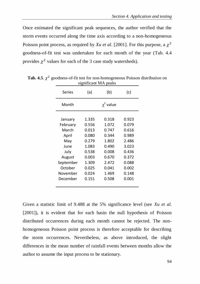
Section 4. Application and testing
94
Once estimated the significant peak sequences, the author verified that the
storm events occurred along the time axis according to a non-homogeneous
Poisson point process, as required by Xu et al. [2001]. For this purpose, a
goodness-of-fit test was undertaken for each month of the year (Tab. 4.4
provides values for each of the 3 case study watersheds).
Tab. 4.5. goodness-of-fit test for non-homogeneous Poisson distribution on
significant MA peaks
Series (a) (b) (c)
Month χ2 value
January 1.335 0.318 0.923
February 0.556 1.072 0.079 March 0.013 0.747 0.616 April 0.080 0.344 0.989 May 0.279 1.802 2.486 June 1.083 0.490 3.023 July 0.538 0.008 0.436
August 0.003 0.670 0.372 September 1.309 2.472 0.088
October 0.025 0.041 0.002 November 0.024 1.469 0.148 December 0.151 0.508 0.001
Given a statistic limit of 9.488 at the 5% significance level (see Xu et al.
[2001]), it is evident that for each basin the null hypothesis of Poisson
distributed occurrences during each month cannot be rejected. The non-
homogeneous Poisson point process is therefore acceptable for describing
the storm occurrences. Nevertheless, as above introduced, the slight
differences in the mean number of rainfall events between months allow the
author to assume the input process to be stationary.

Section 4. Application and testing
95
One major comment is needed about the comparison of the two effective
peaks estimation procedures. As it is possible to realize also by a graphical
analysis of Fig. 4.5 and 4.6, the mean number of significant rainfall events
per year obtained by the MA procedure is considerably higher than that
resulting from the FPOT procedure, for each of the case studies. The values
reported in Tab. 4.5 confirm this consideration.
Tab. 4.6. Mean number of rainfall events per year: comparison between MA and
FPOT procedures
Series (a) (b) (c)
Procedures Mean annual rainfall events
FPOT 17.5 13.1 16.0
MA 39.4 17.9 46.7
In particular, the mean number of events per year obtained by the FPOT
approach confirms the results of Claps and Laio [2005], who reported a
rough estimate of about 5-20 peaks per year for each of the numerous
analyzed runoff series. However, the main point consists in the fact that
authors themselves admitted that such estimation could result in a
underestimation of the actual number of effective rainfall events, suggesting
a clue of the inadequacy of the Poisson independent model in the correct
reproduction of the effective rainfall behavior. The mean number of events
per year obtained by the MA procedure, instead, seems to be much more
compatible with the actual number of events. As a matter of fact, taking the
Alento River as an example, several regional studies undertaken on the

Section 4. Application and testing
96
Italian territory on several uniform compartments (from a hydrological point
of view) seem to confirm the result. In particular, using the Extreme Value-I
(EV-I) distribution for statistical analysis of rainfall heights‟ annual maxima
in intervals of different duration (in the area where the Alento basin is
located), a mean number of events per year equal to 37 was evaluated [Di
Nunno, 1981]. Furthermore, adopting the Two-Component Extreme Value
(TCEV) distribution [Rossi et al., 1984] for the analysis of instantaneous
discharges annual maxima at Casalvelino station (Alento River), a mean
number of flood events per year equal to 44 was estimated [Rossi and
Villani, 1995].
Starting from these considerations, the author considered the MA procedure
more efficient, compared to the FPOT approach, thanks to its ability to
provide a more realistic pulses sequence in terms of mean annual number of
events. It is worth underlying that, on the contrary, a comparison between
FPOT and MA procedures in terms of the mean annual intensity of rainfall
events would be meaningless. Indeed, while the FPOT approach derives the
peak sequence only by means of operation on the recorded runoff series, the
MA procedure provides a sequence, through minimization of Eq. (3.32),
strictly dependent on the values of the estimated parameters of the TF.
Furthermore, given that TFs estimates obtained in this work are considerably
different from those provided by Murrone et al. [1997], concerning the
Alento River, and Claps and Laio [2005], concerning the Scrivia and
Bormida rivers, a comparison between pulses sequence in terms of intensity
would be practically useless.
Eventually, a first way to ascertain, on the one hand, the validity of the
response function form adopted in the calibration approach, and, on the other
hand, the efficiency of the selected MA procedure for the determination of
the effective peaks series, is to provide the reader with a graphical

Section 4. Application and testing
97
comparison between recorded and reconstructed series (Fig. 4.7). The latter
one, in particular, was obtained, for each case study series, through the
convolution (see Eq. 3.34) between the known response function and the
corresponding input sequence. From a quick graphical analysis of the
proposed comparison, it is possible to observe the almost perfect
superimposition of the peak occurrences time between reconstructed and
recorded series, in addition to a practical coincidence between corresponding
discharge values.

Section 4. Application and testing
98
Fig. 4.7. Recorded and reconstructed runoff series comparison – (a) Alento; (b) Scrivia; (c) Bormida

Section 4. Application and testing
99
4.4.1.2. PWNE model parameters estimation
Once selected the MA procedure by Xu et al. [2001] for the estimation of the
significant values of peak rainfall events, given the consideration of
Subsection 4.4.1.1, the PWNE model of effective rainfall was estimated by
the adoption of the method of moments formula of Eqs. (3.31). In particular,
as mentioned in Section 3, starting from the series of significant rainfall
pulses, the parameter , of the Poisson distribution of the occurrences, and
the parameter , of the exponential distribution of the intensities, were
estimated on 13 different seasons of days each, wherein they are
supposed to remain constant. In such a way, the intention of the author was
that of preserving, in the simulated streamflow series, the first-order moment
season variability. Indeed, it is worth underlying that, as stated by some
recent worthy contribution about spectral calibration problems (see, e.g.,
Montanari and Toth [2007]), the PSD of a realization of a stochastic process
does not convey any information about the mean value of the process itself.
As a consequence, in almost all technical papers dealing with spectral
calibration procedures, the authors tend to preserve the mean of the runoff
process through the assumption of zero mean of the model error , which
corresponds to imposing the equality for the mean values of observed and
simulated data [Montanari and Toth, 2007]. However, such a framework can
be easily followed when some information about the input (rainfall,
evapotranspiration etc.) processes are available. When, on the contrary, no
information is obtainable on the input process, the effective rainfall model
parameters estimation becomes fundamental to assure the correct
reproduction of the first moment of the recorded series. As a consequence,
the season length , for the estimation of PWNE parameters and , was set
to 28 days because it was considered the optimal value for the correct

Section 4. Application and testing
100
reproduction of the seasonal variability of the recorded series first order
moment.
Starting from these premises, the parameters estimates of the PWNE model,
for each case study series, are provided in the following Tab. 4.6.
Tab. 4.7. PWNE model parameters estimates
Series (a) (b) (c)
Season #
λ
[1/d] 1/β
[m3/s] λ
[1/d] 1/β
[m3/s] λ
[1/d] 1/β
[m3/s]
1 0.109 165.9 0.054 269.5 0.174 114.7
2 0.067 154.8 0.045 258.8 0.038 1281.8 3 0.086 99.1 0.067 450.4 0.061 824.3
4 0.058 102.5 0.056 386.2 0.063 762.6 5 0.059 43.5 0.048 467.2 0.094 483.8
6 0.024 50.9 0.011 93.9 0.013 635.3 7 0.075 6.5 0.010 106.0 0.034 41.0
8 0.023 17.9 0.010 100.1 0.027 123.2 9 0.091 6.0 0.014 391.3 0.020 256.3
10 0.033 36.3 0.031 766.8 0.037 631.7 11 0.029 129.1 0.073 642.5 0.061 389.8
12 0.090 136.0 0.073 486.4 0.058 1198.8 13 0.142 124.1 0.062 589.4 0.056 1055.4
The universal random variable generator, described in Subsection 3.6, was
thus applied for the generation of synthetic rainfall series, whose statistical
distribution was that of Eqs. (3.29) and (3.30), which were then numerically
convoluted with the discrete time response function of the watershed to
generate synthetic streamflow series. For further details on the simulation
analysis, the interested reader may refer to Subsection 3.6.

Section 4. Application and testing
101
4.4.2. Comparison of main statistical features between recorded and
synthetic streamflow series
4.4.2.1. Introduction
In the present subsection the author will provide the reader with some
interesting comparisons between the generated streamflow series, according
to the procedure exposed in the previous subsections, and the recorded ones,
in order to ascertain the applicability and efficiency of the proposed
frequency-domain calibration procedure. Even though already depicted in
Section 3, it is worth underlying now that, for each case study series, the
generation of 1000 streamflow series of length, in days, was
undertaken, where 364 is the number of days in a year, considering 13
seasons of 28 days each, and is the number of years of the simulation,
assumed in order to double the length of the recorded streamflow series, in
terms of years, . However, before the execution of the statistical
analysis, the first years of the synthetic runoff series were removed, in
order to make generated series independent on the initial conditions of the
simulation.
Concerning statistical analysis, it is widely known that the real value of a
stochastic model must be judged from its capacity of correctly reproducing
the statistical properties of recorded series from which its parameters have
been assessed. As a consequence, as already mentioned at the end of Section
3, the quality of the obtained solution (i.e. TF parameter estimates) was
evaluated in terms of its ability to:
a) reproduce the first three moments, averaged on the different months, of
the recorded series probability distribution;

Section 4. Application and testing
102
b) return an average flow volume, in a period of length equal to , similar
to that corresponding to the recorded series;
c) guarantee a satisfying reproduction of flow duration curves;
d) reproduce minimum and maximum values, averaged on different
aggregation scales, of the recorded series.
4.4.2.2. Comparison of mean statistics
The first validation test, useful to assess the real efficacy of the estimated
watershed response function, concerns the comparison of the moments of the
observed and generated flows, averaged on the different months of the year.
In particular, the author focused on the comparison of the first three
moments of the distribution of the streamflow variable (i.e. mean, standard
deviation and skewness coefficient), whose estimators are provided,
respectively, in the following formulas:
∑
; (4.6)
(
∑
)
; (4.7)
∑
.√
∑
/
; (4.8)
where is the number of elements in the considered sample and is the ith
element of the sample.
The graphical comparison of the aforementioned moments is provided in the
following Fig. 4.8, where upper and lower confidence limits are also
provided by adding and subtracting the standard deviation value to the
corresponding statistic estimate.

Section 4. Application and testing
103

Section 4. Application and testing
104
Fig. 4.8. Comparison of mean statistics of daily flows for each calendar month
between recorded (solid black line) and generated series (solid red line); confidence
intervals ±σ are shown in dashed line – (a) Alento; (b) Scrivia; (c) Bormida
For each of the case study time series, it can be noticed that the overall trend
of the monthly averaged historical moments is quite well preserved by the
generated series. In particular, the best performance concerns the
reproduction of the monthly mean flow values, which confirms the
efficiency of the selected model of effective rainfall. Furthermore, also the
standard deviation and the skewness coefficient overall trends are quite well
preserved. In particular, the former generally presents a negative bias in
correspondence with the tail of the statistics, while both the central and the
extreme portion of the synthetic skewness trends are characterized by a
positive and negative error. Nevertheless, all the synthetic trends are
included in the respective confidence interval represented by the dashed
lines in Fig. 4.8.

Section 4. Application and testing
105
However, in future advances of the calibration procedure here proposed, it
will be attempted to considerably reduce the error in the reproduction of the
mean monthly second order moment, since it is fundamental in simulation
analysis aimed at the reproduction of the correct discharge trend within a
month. The reader should think, for instance, to a typical water resource
management problem of an artificial reservoir. As a matter of fact, in this
case, in order to define the best rule for the management of water volumes
stored in the reservoir during the year, it is fundamental the availability of a
stochastic model for the correct reproduction of the streamflow process
within the year. In particular, the shorter is the aggregation scale within
which the model is able to reproduce the streamflow variability, the more
detailed will be the estimated reservoir scheduling.
The second validation test, in terms of mean statistics, concerns the
comparison of the total historical flow volume, that corresponds to the
recorded streamflow series of length , with the average of the 1000 total
flow volumes corresponding to the simulated runoff series of the same
length (Tab. 4.7 provides the comparison for each case study series). The
importance of this test is intuitive, given the evident necessity of a correct
reproduction of this statistic in water resources management problems on a
over-year time scale.

Section 4. Application and testing
106
Tab. 4.8. Recorded and mean synthetic flow volumes comparison for each case
study series
Series Rec. flow vol. [m3] Mean synt. flow vol. [m3] % error
(a) 2.24 x 10⁹ 2.32 x 10⁹ -3.6
(b) 6.61 x 10⁹ 7.01 x 10⁹ -6.0
(c) 9.07 x 10⁹ 9.61 x 10⁹ -5.9
Tab. 4.7 demonstrates the capacity of the identified watershed models to
properly reproduce, with an acceptable error, the total flow volume on a
period of length equal to . In particular, for each of the watersheds, the
slightly overestimation of the recorded flow volume was probably due to the
uncertainty both in the effective rainfall model parameters estimations and in
the subsequent rainfall series synthetic generation.
4.4.2.3. Comparison of flow-duration curves
The flow-duration curve is a cumulative frequency curve that shows the
percent of time during which specified discharges were equalled or exceeded
during a given period. It combines in one curve the flow characteristics of a
stream throughout the range of discharge, without regard to the sequence of
occurrence. To prepare a flow-duration curve, the mean daily, weekly, or
monthly flows during a given period are arranged according to their
magnitude, and the percent of time during which the flow variable equals or
exceeds the specified values is computed. The curve, drawn to average the
plotted points of specified discharges versus the percent of time during
which they were equalled or exceeded, thus represents an average for the

Section 4. Application and testing
107
period considered rather than the distribution of flow within a single year
[Searcy, 1959].
It is widely recognized the utility of flow-duration curves in several
applications. In particular, in this thesis, they were adopted to properly
compare the observed and synthetic cumulative distribution functions of the
streamflow process, of which flow-duration curves can be considered an
appropriate representation.
Estimation of flow-duration curves was undertaken by the adoption of the
procedure, described by Claps et al. [2005], described in the following lines.
Concerning the observed discharge series, the historical dataset of size ,
where is the length of the series in days, was sorted in descending order
and an empirical frequency of occurrence, equal to
was assigned
to the ith order statistics in the sample, that is ( ). The same
procedure was followed for the whole generated runoff series, given by
merging the 1000 synthetic series, each of length , in an unique generated
series. As a result, the size of the synthetic series was much larger than .
Hence, the empirical frequency of occurrence was estimated as
and the jth order statistics in the sample was evaluated as ( ),
where the apex is used to distinguish synthetic streamflow data from
recorded ones. Eventually, the flow-duration curves were given by the
and values, on the abscissa, plotted versus, respectively, and on
the ordinate. The graphical comparison between recorded and synthetic
series flow-duration curves is provided in the following figure, for each case
study watershed. It is worth noticing that, in order to allow the representation
of the frequency axis in terms of number of days in the year, it is only
needed to multiply by 365 the frequency of occurrence values on the
abscissa

Section 4. Application and testing
108

Section 4. Application and testing
109
Fig. 4.9. Comparison between flow-duration curves of recorded (solid line) and
simulated (dotted line) series – (a) Alento; (b) Scrivia; (c) Bormida
Figs. 4.9a-c clearly show the considerable result obtained in terms of
matching of the global trend of the recorded runoff series flow-duration
curves for the Alento and Bormida rivers, both for the lower (less frequent
and, thus, more relevant flow events) and the upper (more frequent discharge
values) tails of the frequency distribution. A certain difference, instead, can
be noticed between the two curves concerning the Scrivia River (Fig. 4.9b).
In particular, a low underestimation of the highest flow values (i.e. the rarest
events) and a moderate overestimation of the lowest discharges (i.e. the
runoff during long dry periods) is revealed. Such a difference could be
addressed to the absence, in the time response function identified for the
Scrivia watershed, of a strong impulsive contribution. As a matter of fact,
given the results shown in Tab. 4.2, while for the Alento and Bormida rivers
this component is respectively equal to about the 16% and 12% of the total
Section 4. Application and testing
110
discharge, for the Scrivia River the direct runoff is only the 2% of the total.
This substantial difference can particularly affect the capacity of the
calibrated response function of properly reproducing both the dry periods
runoff values and the rarest events. In particular, in presence of response
functions similar to that of the Scrivia River, when a high intensity effective
rainfall event is generated by the universal random variable generator
described in Section 3, the resulting runoff value will not be characterized by
a relevant magnitude, since the absence of a considerable impulsive
contribution results in the fact that only a small portion of the effective
rainfall feeds the runoff process. At the same time, given that the greatest
amount of rainfall contribution feeds the over-month and over-year storage
capacities of the watershed, the direct consequence will be an overestimation
of more frequent (i.e. with minor intensity) flow values, since they are
affected by that amount of previous intense rainfall events that have been
preliminary stored in the several watershed capacities, and, after, slowly
released to the river. Such an interesting result would suggest the adoption of
a different response function form for the Scrivia River, in order to
differently model the surface runoff. For instance, the Dirac delta function
could be substituted by 2 or 3 identical linear reservoirs, obtaining a
response function able to release in a wider time interval the quick runoff
contribution [see, for reference, Boyle, 2000]. However, in this direction
further investigation need to be pursued to improve the overall capacity of
the proposed approach to properly fit the upper and lower tails of the
recorded flow-duration curves.
The different performances, of the proposed calibration approach, in the
reproduction of the cumulative distribution functions of the recorded
streamflow processes, could result in troublesome limitations to the adoption
of the methodology in water resources management problems. Indeed, for

Section 4. Application and testing
111
instance, the management of an artificial reservoir at a short time-scale
would require the ability of the stochastic model, for the generation of
synthetic streamflow series, of correctly reproducing the high frequency
values, given their importance in the definition of a short time-scale
scheduling of the reservoir. However, it is also true that, as already shown in
Tab. 4.7, all the calibrated response function are able to correctly reproduce,
with a limited error, the global flow-volume in the recording period,
suggesting the model ability in reproducing the real flow regime on an
extended period. Such a result is not contrasting with the flow-duration
curve of the Scrivia River (Fig. 4.9b), since the underestimation of the high
frequency discharge values and the overestimation of the low frequency ones
results in a global trade-off in terms of flow-volume, providing the results
shown in Tab. 4.7.
4.4.2.4. Reproduction of minimum flow values over fixed durations
As already said, one of the main applications of streamflow processes
stochastic models is the possibility to generate synthetic streamflow series to
cope with a wide variety of water resources problems. In particular, one of
the most popular class of problems, to which synthetic models have been
usually applied, deals with water resources planning and management, e.g.
the determination of the best artificial reservoir operating rule curve within a
year or in a multi-year framework. As already stated, it is intuitive that, in
this type of applications, stochastic models have to be able to correctly
reproduce the main distribution properties of the recorded series from which
they have been calibrated. In previous subsections, indeed, several validation
tests have been provided, comparing recorded and generated series in terms
of, in particular, the first three moments of the distribution, the global flow-

Section 4. Application and testing
112
volume over a given period and flow-duration curves. All these tests showed
satisfying results. However, it is worth underlying that, in almost all
practical problems to which a stochastic streamflow model can be applied,
the proper reproduction, in statistical terms, of minimum flow values would
be a significant characteristic of the adopted model. For this reason, in the
present subsection, the graphical comparison between recorded and
simulated mean minimum flows, averaged over different durations, is
provided.
For the sake of repeatability, the author will firstly describe how to estimate
mean minimum flow values, given a series of mean daily flows of
values. Defined a certain duration (in days), a new series is obtained by
averaging the groups of flows, each characterized by daily flow values,
obtained by dividing the historic sequence in ⁄ portions. The
minimum value of the series thus obtained is the mean minimum flow value
for the fixed duration . The same procedure needs to be followed both for
recorded and synthetic series (that in the present work are 1000 for each case
study river). In this latter case, in particular, once repeated, for the a fixed
duration the previous procedure for each of the generated series, the mean
minimum flow to be compared to that corresponding to the recorded series,
for the same duration , is evaluated by averaging the 1000 mean minimum
values obtained by the synthetic series. Fig. 4.10 shows results for each case
study watershed.
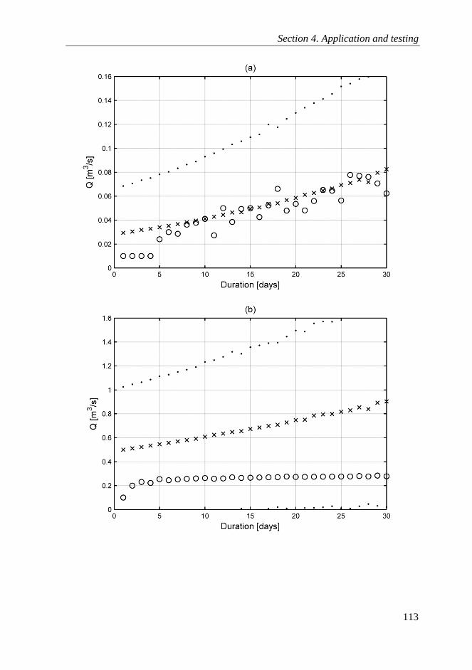
Section 4. Application and testing
113

Section 4. Application and testing
114
Fig. 4.10. Comparison of minimum mean discharges, averaged over different
durations, between recorded (circle points) and synthetic (cross points) series with ±
2σ confidence limits (dotted points) – (a) Alento; (b) Scrivia; (c) Bormida
From a first graphical analysis of Fig. 4.10, one should notice that, for each
case study, the recorded and generated series trends are both included within
the confidence bands (following Murrone et al. [1997]). In particular, the
best performance is that obtained for the Alento riverflow series, where an
almost perfect superimposition of recorded and generated mean minimum
flow values was obtained for each duration from 1 to 30 days. However,
within the same case study, it has to be noticed the poorest results, if
compared to those obtained for the other durations, are those pertinent to the
shortest durations (from 1 to 4 days). The author connects this result to the
adopted effective rainfall model (the so-called PWNE model) that, most
likely, is not able to properly reproduce shortest-time statistical features
given the limitation in the number of its parameters.

Section 4. Application and testing
115
Considerably different results were instead achieved concerning the Scrivia
(Fig. 4.10b) and Bormida (Fig. 4.10c) case study rivers. In the former case,
indeed, it is possible to notice a certain increasing overall trend, for the
synthetic streamflow series, in the mean minimum values from lowest to
highest durations. On the contrary, the same trend is not recognizable for the
recorded series, where, instead, the mean minimum flow value remains
almost constant. This result is easily explicable by means of a detailed
analysis of the Scrivia recorded streamflow series. As a matter of fact, from
the corresponding 14 recording years, it is possible to notice a particularly
long and anomalous dry period (that is, with a mean daily flow value minor
than 0.5 ⁄ ) from the second half of July to the first half of October, of
the thirteenth year of the recorded sequence. As obvious, given that the
parameters of the PWNE model, of the effective rainfall, had been estimated
as mean values on each month of the year, they were not able to take into
consideration of such an atypical occurrence, determining the evident
difference in the global trend shown in Fig. 4.10b.
A considerable different situation concerns, instead, the Bormida River case
study. As a matter of fact, Fig. 4.10c clearly shows an underestimation of the
mean minimum flow values of the recorded series by the generated ones, for
each duration . Nevertheless, the overall increasing trend is quite similar to
that of the historical sequence. However, it is evident the inability of the
model in reproducing the considerable “peaks”, of the mean minimum flow
values, for some of the considered averaging durations, given that, as
confirmed also by Fig. 4.10a-b, the model is only able to reproduce a regular
increasing path of the minimum values over fixed durations. Such a limit is
to be related to the aforementioned estimation procedure of the parameters of
the PWNE model of the effective rainfall. As a matter of fact, the estimation
of the couple of parameters and on 13 “season”, each of 28 days of

Section 4. Application and testing
116
length, does not allow the correct reproduction of those particular
streamflow events that can result in the “peaks” provided by Fig. 4.10c.
Hence, synthetically, results obtained by the comparison of mean minimum
flows, averaged over different durations, between historical and generated
series, provide that the calibrated model is able to satisfactory reproduce the
recorded series path if two conditions are verified (see Fig. 4.10a concerning
the Alento River):
- the absence, in the historical sequence, of singular long dry periods, which
could be considered anomalous if compared to the standard dry periods;
- the absence of singular streamflow events, whose high intensity of the
rainfall events, from which it originates, could be barely reproduced by the
mean estimates of the parameter of the adopted model for the effective
rainfall reproduction.
In order to overcome these limitations, the author is confident that the
adoption of a more complex models for the reproduction of the effective
rainfall phenomenon (e.g., the five-parameters Neyman-Scott cluster model)
can be decisive. However, further analysis will be necessary in the
immediate future to confirm this idea.

Section 5. Conclusions
117
5. Conclusions
5.1. Thesis summary
In this thesis, a frequency-domain calibration procedure of SN-based models
for streamflow modeling has been studied. It is now worthwhile to review
the most important results and considerations achieved in the different
sections of the thesis.
Section 2 has been devoted to provide the reader with a comprehensive and
synthetic review of the techniques, available in the technical literature,
aimed at the calibration of CT model. The first part of the section has been
addressed to the definition of the major advantages of the application of a
CT identification framework compared to a DT one, resulting in the general
convenience of the former class of approaches. Subsequently, in a first
subsection, a short survey of time-domain methods for the identification of
CT models has been provided, while in a successive subsection the class of
frequency-domain identification procedures has been dealt with. Finally, the
two main advantages of the latter class of methods have been discussed, that
can be summarized as:

Section 5. Conclusions
118
(a) the possibility to replace large data sets, usually necessary in a time-
domain framework, with a limited number of frequency-domain information
on input and output signals;
(b) the possibility of combining data collected from different experiments
that, on the contrary, is not easily possible in time-domain data procedures.
Section 3 has focused on that class of CT models known as Shot Noise (SN).
In particular, in a first subsection, a comprehensive survey of the literature
contributions to the topic has been provided, recognizing the model ability in
the reproduction of short time scale discharge series, due to its aptitude to
properly reproduce the presence of peaks and recessions, characteristic of
daily discharge time series. Furthermore, a detailed mathematical description
of SN processes, and relative properties, has been addressed. Particular
attention has been paid to their spectral properties, which allow one to avoid
the adoption of input processes data (e.g., rainfall series, evapotranspiration
series etc.) in the calibration procedure presented in this thesis, which can be
sees as the main contribution of the whole work, especially if compared to
previous identification approach of SN models in the frequency domain.
Furthermore, after an overview on classical time-domain calibration
procedures, the proposed spectral-domain calibration method has been
presented. The objective response function, to be identified, is given by the
linear combination of three parallel linear reservoirs, each with a different
storage coefficient (representing the several groundwater contributions), and
a fast surface runoff contribution. In order to estimate the response function
parameters, the given procedure consists in a least-square fitting of the
streamflow process PSD, through the squared module of the model TF, with
unknown parameters. The form of the watershed response function has been
thus provided, in order to allow proper definition of the unknown

Section 5. Conclusions
119
parameters. Moreover, some details on the available techniques for the
estimation of the output process PSD have been provided, focusing, in
particular, on the selected maximum entropy (or all-poles) approximation.
The last part of Section 3 has dealt with the description of the PWNE model
for the modeling of effective rainfalls. In particular, method of moments
formulas for the estimation of its two parameters have been provided.
Moreover, a description of the methods, available in the scientific literature,
for the assessment of the effective pulses sequence has been addressed.
Particular attention has been paid to the description of the so-called FPOT
and MA procedures.
Eventually, the application and testing of the proposed calibration procedure
have been addressed in Section 4. A detailed description of the three selected
riverflow time series has been provided in a first subsection, highlighting the
differences, in terms of climatic features, among the corresponding
watersheds. In particular, two rivers associated to watersheds mostly
influenced by the climate of the Alps (Scrivia and Bormida) and one
characterized by a maritime rainfall regime (Alento) have been selected.
Thus, once provided some details on the multidimensional minimization
approach selected for the least-square minimization of the cost function (i.e.
the so-called Powell‟s method), estimations of the parameters value have
been provided, together with the graphical result of the streamflow process
PSD through the squared module of the TF.
Subsequently, in order to allow the overall quality of the obtained response
function, a simulation analysis, consisting in the generation of 1000
synthetic streamflow series for each case study watershed, has been needed.
For this purpose, the selection of the most suitable technique for the
assessment of the sequences of effective rainfall pulses has been necessary.

Section 5. Conclusions
120
Concerning this point, a detailed comparison, in terms of reproduction of the
statistical features of the effective rainfall phenomenon, between the
aforementioned FPOT and MA procedures has been undertaken. Obtained
results have suggested the general convenience in the adoption of the latter
approach, especially thanks to its capacity in the reproduction of the correct
number of peak events per year.
Finally, statistical analysis on the generated series have been executed and
reported in the last subsections of Section 4, in order to assess the overall
quality of the obtained calibrations. In particular, the following synthetic
results have been reported.
The estimated response functions have shown a certain effectiveness in the
reproduction of the overall trend of the first three moments of the
distribution, of the recorded streamflow series, averaged over the different
months of the year. In particular, only a slight negative bias in the
reproduction of the tails of the standard deviation of the distribution has been
noticed, for all the case study series. Furthermore, the capacity in the
reproduction of the total flow-volume in a certain period of observation has
been evaluated. Results, provided in Section 4, have clearly shown a
maximum overestimation equal to 6% of the total flow-volume, confirming
the relevance, of the calibrated response function, in water resources
management problems.
Moreover, other two statistical tests have been undertaken on the generated
series. Firstly, Section 4 reports the comparison between recorded and
generated series flow-duration curves, considered as an expression of their
cumulative distribution functions. As clearly shown, the overall trend of the
curve is quite well reproduced for all the three case studies. However,
concerning the Scrivia River, a moderate underestimation (overestimation)
of lowest (highest) frequency values is shown. Such a result has been

Section 5. Conclusions
121
addressed to the presence, in the estimated response function, of a small
direct runoff contribution, if compared to other groundwater components,
which could suggest the adoption of a different modeling, in the response
function form, of the direct runoff (e.g., by means of one or a cascade of
identical linear reservoir).
At last, the capacity in the reproduction of minimum mean flow values,
averaged over different durations (from 1 to 30 days), has been investigated.
Remarkable results have been obtained for the Alento River, while some
problems have arisen from the Scrivia and Bormida. As a matter of fact, in
the former case, the model has not been able to “read” the presence, in the
historical series, of an anomalous long dry period (which results in a
constant trend of minimum mean flow values over different durations).
While, concerning the Bormida River, even though the overall increasing
trend has been correctly reproduced, the estimated solution has resulted
unsuitable for the reproduction of the “peaks” in the minimum mean
discharges, especially for the highest duration values. Both Scrivia and
Bormida rivers unsatisfactory results have been related to the effective
rainfall model estimation technique adopted in the thesis, which estimates
the two parameter values of the PWNE model as mean values over 13
periods of 28 days each, in order to preserve the seasonal variability of the
input process.
5.2. Further developments
Several aspects of the proposed work can be object of future developments
to improve the quality of the presented calibration approach.
A first considerable contribution could concern the form of the response
function, and thus of the corresponding TF, adopted in the frequency-domain

Section 5. Conclusions
122
fitting of the streamflow process PSD. Indeed, as deeply outlined in Section
4, the poor results, in the reproduction of the historical flow-duration curve
for the Scrivia River, are especially due to the absence of a strong direct
runoff contribution. As a consequence, the adoption of a different response
function form (e.g., with the direct runoff modeled by means of a cascade of
2 or 3 identical linear reservoirs) would result in different parameters
estimate and, probably, in a better reproduction of the historical flow-
duration curve.
A second relevant, and probably more effective, development could deal
with the application of an alternative model for the effective rainfall process
modeling. Indeed, as outlined in the previous subsection, some of the
differences between recorded and simulated runoff series have been
addressed to the implicit limitations in the adoption of the PWNE model. As
a consequence, it appears that the adoption of a more complex model,
characterized by a greater number of parameters (e.g., the five parameters-
Neyman-Scott model with exponential instantaneous pulses, within a shot-
noise model of daily streamflows), could result in a better reproduction of
the real dynamics of the effective rainfall process, thus allowing the better
fitting of the streamflow process statistics.
Eventually, the intention of the author is to adopt the know-how acquired for
the development of the present thesis to the resolution of problems
concerning the frequency-domain calibration of hydrologic models, not only
in a SN framework.

Appendix
123
Appendix
The aim of the present brief appendix is to clarify some fundamental issues
to allow the reader a comprehensive understanding of some basilar concepts
addressed in this thesis.
In the technical literature, a large variety of models is available for the
description of rainfall-runoff transformations, each one suitable for the
resolution of a particular class of hydrologic issue. Moreover, several
authors attempted to classify rainfall-runoff models [e.g., Todini, 1988],
even in absence of an universal criterion of classification. Among them,
however, each existing classification recognizes the importance of the so-
called lumped-conceptual models. Conceptual models are those determined
by the arrangement of a small number of elements, each characterizing the
simple representation of a physical relationship [Dooge, 1959]. Lumped
models, instead, refer to the fact that the model parameters are averaged on
the entire watershed [Troutman, 1985]. Among lumped-conceptual models, a
great interest has always been received by the so-called Linear
Compartmental Systems (LCSs) [Jacquez, 1985], given by the parallel
and/or cascade connection of a certain number of linear reservoirs, i.e.
subsystems characterized by a negative exponential impulse response. Some
applications of this category of models within stochastic streamflows

Appendix
124
generation problems are provided by Murrone et al. [1997], Boyle [2000]
and Claps et al. [2005]. These models are usually characterized by two main
properties:
- linearity: that is, the response of the model to a linear combination of two
valid inputs is equal to the linear combination of the single response of the
model to each input;
- time invariance: that is, the model parameters remain constant with the
time.
The validity of the given properties leads to the definition of the so-called
Linear Time Invariant (LTI) models, that can be synthetically defined as
those systems where at any time instant the current value of the output
process, , can be obtained as a linear combination of present and past
input process, , values [Priestly, 1981, Section 1]. According to this
assumption, in the case of LTI models, the relationship between input and
output signals can be expressed in the following form:
∫
(A.1)
where the function , known as impulse response function, describes the
form of the output of the system when the input is an unit impulse function
(that is a function which take a very large value at just one time point, is
almost zero everywhere else, and has an unit area) centred at the origin
[Priestly, 1981, Section 1].
From the definition (A.1), the Transfer Function (TF), of the LTI system, is
a complex valued function obtained by the bilateral Laplace transform,
{ }, of the impulse response function [Kailath et al., 2000, Chapter 6]:

Appendix
125
{ } ∫
(A.2)
where (with the imaginary unit), known as complex or Laplace
variable, defines the complex plane (i.e. the existence domain of the TF,
characterized by a x, or real-axis, , and a y, or imaginary-axis, , also
known as frequency, , axis).
Given the TF form (A.2), the corresponding frequency response, , is
obtainable by the restriction of the Laplace domain to the points belonging to
its positive-imaginary semi-axis (thus substituting for in the TF
expression, setting the real part of the complex variable to zero) [Sourdille
and O'Dwyer, 2004]. Hence, the frequency response function can be defined
as the Fourier transform of the impulse response function [Jenkins and
Watts, 1968, Subsection 2.3]. It is worth noticing that, in many identification
problems, it is convenient to refer to the rational form of the frequency
response, given by the following expression:
∑
∑
(A.3)
where and are, respectively, numerator and denominator of the
frequency response, defined as a function of the two polynomials of real
parameters and . In particular, if these latter are coprime, i.e. they have
no factors in common, the roots of and are called, respectively, zeros
and poles of the system (also known as singularities of the TF) [Kailath et
al., 2000, Chapter 6].
The two aforementioned functions, and , are fundamental in the
analysis of LTI systems. As a matter of fact, if one assumes that the input
consists of a sum of harmonic functions with different frequencies ,

Appendix
126
the output from the LTI system will similarly consists of a sum of harmonic
functions with exactly the same frequencies. At each frequency, however,
the harmonic functions result scaled in amplitude by a certain factor
(known as gain or magnitude function) and shifted in phase by an amount
(called phase angle function) [Jenkins and Watts, 1968, Subsection
2.3]. The TF of Eq. (A.2), or equivalently the corresponding frequency
response function of Eq. (A.3), simply provides how, for each , the
amplitude (and phase) of an input harmonic signal of that frequency is
transformed into the amplitude (and phase) of the corresponding output
wave [Priestly, 1981, Section 1].
In system identification theory, it is conventional to plot the gain function
, expressed in decibel (that is, multiplying by 20 the decimal logarithm
of the considered amount), against the logarithm of the frequency , and the
phase function against the logarithm of the frequency. These
diagrams, known as Bode plots, allow one to graphically understand the
behaviour of the system in terms of transformations of both gain and phase
angle features of the harmonics that characterize the input signal , and
their aspect is determined by the combination of poles and zeros of the TF in
terms both of their typology (real or complex conjugate) and of their sign
(positive or negative) (for a comprehensive description of Bode plots and
their utility in system identification theory, refer to Bolzern et al. [2004,
Subsection 6.6.1]). Furthermore, some interesting examples of Bode plots,
for different types of TFs with different combinations of its poles and zeros
values, are provided by Jenkins and Watts [1968, Subsection 2.3].

References
127
References
Ahmed, J. A., and A. K. Sarma (2005), Genetic Algorithm for Optimal
Operating Policy of a Multipurpose Reservoir, Water Resources
Management, Volume 19, Number 2, pp. 145-161.
Aksoy, H. (2003), Markov chain-based modeling techniques for stochastic
generation of daily intermittent streamflows, Adv. Water Resour., 26, pp.
663–671.
Anderson, B. (1985), Identification of scalar errors-in-variables models with
dynamics, Automatica, 21, (6), pp. 709–716.
Astrom, K. J. (1969), On the choice of sampling rates in parametric
identification of time series, Information Sciences 1 (1), 273-278.
Bandini, A. (1931), Tipi pluviometrici dominanti nelle regioni italiane,
Servizio Idrografico Italiano, Roma (in Italian).
Battaglia, F. (1986), Modelli stocastici per la rappresentazione e la
previsione dei deflussi, Dept. of Statistics Papers, No. 3, Univ. di Roma "La

References
128
Sapienza”, Dip. di Statistica, Probabilità e Statistica Applicata, Rome (in
Italian).
Bayazit, M., and H. Aksoy (2001), Using wavelets for data generation. J
Appl Stat, 28(2): 157–166.
Bernier, J. (1970), Inventaire des modeles de processus stochastiques
applicables a la description des debits journaliers des rivieres, Revue Inst
Intern Stat; 38(1): 49–61.
Bloeschl, G., and M. Sivapalan (1995), Scale issues in hydrological
modelling: A review, Hydrol. Processes, 1995, 9, 251– 290.
Bo, Z., S. Islam, and E. A. B. Elthair (1994), Aggregation-disaggregation
properties of a stochastic rainfall model, Water Resour. Res. 30(12), 3423-
3435.
Bolzern, P., R. Scattolini, and N. Schiavoni (2004), Fondamenti di controlli
automatici, II edition, McGraw Hill, Milano (Italy) (in Italian).
Boughton, W. C., and O. P. Droop (2003), Continuous simulation for design
flood estimation - a review, Environ. Model. Softw., 18 (4), 309-318.
Box, G. E. P., G. M. Jenkins, and G. C. Reinsel (1994), Time Series
Analysis, Forecasting and Control, (third ed.) Englewood Cliffs, New Jersey,
Prentice Hall.

References
129
Boyle, D. P. (2000), Multicriteria calibration of hydrological models, Ph. D.
dissertation, Dep. of Hydrol. and Water Resour., Univ. of Ariz., Tempe.
Broersen, P. M. T. (1995), A Comparison of Transfer Function Estimators,
IEEE Transactions on Instrumentation and Measurements, vol. 44, no. 3, pp.
657-661.
Burg, J. P. (1975), Maximum entropy spectral analysis, Ph. D. Thesis,
Stanford University, Palo Alto., California.
Castiglioni, S., L. Lombardi, E. Toth, A. Castellarin, and A. Montanari
(2010), Calibration of rainfall-runoff models in ungauged basins: A regional
maximum likelihood approach, Adv. Water Resour., 33,1235–1242.
Chang, L. C, and F. J Chang (2001), Intelligent control for modeling of real
time reservoir operation, Hydrological Processes, 15, pp. 1621–1634.
Claps, P., A. Giordano, and F. Laio (2005), Advances in shot noise modeling
of daily streamflows, Adv. Water Resour., 28: 992–1000.
Claps, P., and F. Laio (2003), Can continuous streamflow data support flood
frequency analysis? An alternative to the partial duration series approach,
Water Resour. Res., 39 (8), p. 1216.
Claps, P., F. Rossi, and C. Vitale (1993), Conceptual-stochastic modeling of
seasonal runoff using Autoregressive Moving Average Models and different
scales of aggregation, Water Resour. Res. 29(8), 2545-2559.

References
130
Cowpertwait, P. S. P. and P. E. O'Connell (1992), A Neyman-Scott shot
noise model for the generation of daily streamflow time series, Advances in
Theoretical Hydrology, Part A, Chap. 6. Elsevier, The Netherlands.
Di Nunno, U. (1981), Analisi statistica delle massime piogge in Campania,
Unpublished thesis, University of Naples (in Italian).
Diskin, M. H. (1964), A basic study of the linearity of the rainfall-runoff
process in watersheds, Ph. D. thesis, Dep. of Civ. Eng., Univ. of Ill., Urbana.
Diskin, M. H. and G. G. S. Pegram (1987), A study of cell models: 3. A pilot
study on the calibration of manifold cell models in the time domain and in
the Laplace domain, Water Resour. Res., Vol.23, No.4, pp.663-673.
Dooge, J. C. I. (1959), A general theory of the unit hydrograph theory, J.
Geophys. Res. 64 (2), 241–256.
Eagleson, P. S. (1978), Climate, soil, and vegetation: 2. The distribution of
annual precipitation derived from observed storm sequences, Water Resour.
Res., 14(5), 713-721.
Efstratiadis, A., Y. G. Dialynas, S. Kozanis, and D. Koutsoyiannis (2014), A
multivariate stochastic model for the generation of synthetic time series at
multiple time scales reproducing long-term persistence, Environmental
Modelling and Software, 62, 139–152.
Eykhoff, P. (1974), System identification, Wiley, New York.

References
131
Hino, M. and M. Hasebe (1981), Analysis of hydrologic characteristics from
runoff data - A hydrologic inverse problem, Jour. of Hydrol., 49(3/4), 287-
313.
Hino, M., and M. Hasebe (1984), Identification and prediction of nonlinear
hydrologic systems by the filter-separation autoregressive (AR) method:
extension to hourly hydrologic data, Jour. of Hydrol., 68: 181-210.
Hipel, K. W., and A. I. McLeod (1994), Time Series Modeling of Water
Resources and Environmental Systems, Elsevier, Amsterdam.
Ilich, N. (2014), An effective three-step algorithm for multi-site generation
of weekly stochastic hydrologic time series, Hydrol. Sci. J., 59 (1), 85-98.
Islam, M., and B. Sivakumar (2002), Characterization and prediction of
runoff dynamics: a nonlinear dynamical view, Advances in Water
Resources, 25(2): 179–190.
Jacquez, J.A. (1985), Compartmental analysis in biology and medicine, 2nd
edition (Ann Arbor: University of Michigan Press).
Jenkins, G. M., and D. G. Watts (1968), Spectral Analysis and Its
Applications. Holden-Day, 525 pp.
Kailath, T., A. H. Sayed, and B. Hassibi (2000), Linear estimation, Prentice-
Hall, Upper Saddle River, NJ.

References
132
Kallstrom, C. G., T. Essebo, and K. J. Astrom (1976). A computer program
for maximum likelihood identification of linear multivariable, stochastic
systems, Proc. 4th IFAC, Symposium on Identification and System
Parameter Estimation, Tbiliss.
Karamouz, M., and M. H. Houck (1987), Comparison of stochastic and
deterministic Dynamic programming for reservoir operating rule generation,
Water Resources Bulletin, Bethesda, v. 23, n. 1, p. 1-9.
Karamouz, M., M. H. Houck, and J. W. Delleur (1992), Optimization and
simulation of multiple reservoir systems, Journal of Water Resources
Planning and Management, Vol. 118 (1).
Kavvas, M. L. and J. W. Delleur (1981), A stochastic cluster model of daily
rainfall sequences, Water Resour. Res, 17(4), 1151-1160.
Kirchner, J. W., X. Feng, and C. Neal (2000), Fractal stream chemistry and
its implications for contaminant transport in catchments, Letters to Nature,
403: 524–527.
Koch, R. W. (1985), A stochastic streamflow model based on physical
principles, Water Resour. Res., 21(4): 545–53.
Labat, D., R. Ababou, and A. Mangin (2000), Rainfall–runoff relations for
karstic springs. Part II: Continuous wavelet transform and multiresolution
analyses, J. Hydrol., 238, 149–178.

References
133
Lall, U., and A. Sharma (1996), A nearest neighbor bootstrap for resampling
hydrologic time series, Water Resour. Res., 32(3), 679–693.
Ljung, L. (1987), System identification: theory for the user, Prentice-Hall,
Inc, Englewood Cliffs, NJ.
Montanari, A., and E. Toth (2007), Calibration of hydrological models in the
spectral domain: An opportunity for ungauged basins?, Water Resour. Res.,
43, W05434.
Muratori, S., C. Piccardi, and S. Rinaldi (1992), On the minimum phase of
compartmental systems, Int. J. Control., 56, pp. 23–34.
Murrone, F., F. Rossi, and P. Claps (1997), Conceptually-based shot noise
modeling of streamflows at short time interval, Stoch. Hydrol. Hydrau.,
11:483–510.
Nikias, C. L., and J. M. Mendel (1993), Signal processing with higher-order
spectra, IEEE Signal Processing Magazine, 1053-5888.
O'Connell, P. E., and D. A. Jones (1979), Some experience with the
development of models for the stochastic simulation of daily flows, Inputs
for Risk Analysis in Water Resources, pp. 287-314, Water Resour. Publ.,
Fort Collins, CO.
Ouarda, T. B. M. J., J. W. Labadie, and D. G. Fontane (1997), Indexed
sequential hydrologic modeling for hydropower capacity estimation, Journal
of the American Water Resources Association, 33 (6), pp. 1337–1349.
References
134
Papoulis, A., and S. U. Pillai (2002), Probability, Random Variables, and
Stochastic Processes, McGraw-Hill, New York.
Parajka, J., R. Merz, and G. Bloeschl (2005), A comparison of
regionalization methods for catchment model parameters, Hydrol. Earth
Syst. Sci., 9, 157–171.
Pegram, G. G. S. (1980). A continuous streamflow model, Journal of
Hydrology, Vol.47, pp. 65-89.
Penta, A., and F. Rossi (1979), Appunti di idrologia – Parte I: caratteristiche
dei bacini idrografici, Università di Napoli, Facoltà di Ingegneria, Istituto di
Idraulica e Costruzioni Idrauliche. (in Italian).
Pintelon, R., P. Guillaume, Y. Rolain, J. Schoukens, and H. Van Hamme
(1994), Parametric identification of transfer functions in the frequency
domain - A survey, IEEE Trans. Autom. Control, 39, (11), pp. 2245-2260.
Post, D. A., and A. J. Jakeman (1999), Relationships between catchment
attributes and hydrological response characteristics in small Australian
mountain ash catchments, Hydrol. Processes, 10, 877– 892.
Powell, M. J. D. (1964), An efficient method for finding the minimum of a
function of several variables without calculating derivatives, Comput. J., 7:
155-162.

References
135
Prairie, J. R., B. Rajagopalan, T. J. Fulp, and E. A. Zagona (2006), Modified
K-NN model for stochastic streamflow simulation, J. Hydrol. Eng., 11(4),
371–378.
Press, W.H., S. A. Teukolsky, W. T. Vetterling, and B. P. Flannery (1996),
Numerical Recipes in Fortran 77: The Art of Scientific Computing, 2nd ed.,
Cambridge University Press, New York.
Priestly, M. B. (1981), Spectral Analysis and Time Series, London, England,
Academic Press.
Raman, H., and N. Sunilkumar (1995), Multivariate modeling of water
resources time series using artificial neural network, Hydrol Sci J 40(2):
145–163.
Rao, G. P., and H. Unbehauen (2006), Identification of continuous-time
systems, IEE Proc. - Control Theory Appl., 152, 185-220.
Roberts, J. B. (1965), The response of linear vibratory systems to random
impulses, Journal of Sound and Vibration 2, 375-390.
Rodriguez-Iturbe, I., D. L. Cox, and V. Isham (1987), Some models for
rainfall based on stochastic point processes, Proc. R. Soc. Lond. A 410, 269-
288.
Rossi, F., and P. Villani (1995), Leggi regionali di crescita con il periodo di
ritorno. Valutazione delle Piene in Campania, C.N.R. Report, Rossi and
Villani (Eds.), 99-162 (in Italian).

References
136
Rossi, F., M. Fiorentino, and P. Versace (1984), TCEV distribution for flood
frequency analysis, Water Resour. Res., 20(7): 847-856.
Schaefli, B., and E. Zehe (2009), Hydrological model performance and
parameter estimation in the wavelet-domain, Hydrol Earth Syst Sci,
13:1921–36.
Schoukens, J., R. Pintelon, and H. Van Hamme (1994), Identification of
linear dynamic systems using piecewise constant excitations: use, misuse
and alternatives, Automatica, 30, (7), pp. 1153–1169.
Searcy, J. K. (1959), Flow duration curves, U. S. Geological Survey Water.
Seibert, J., and J. J. McDonnell (2002), On the dialog between
experimentalist and modeler in catchment hydrology: use of soft data for
multicriteria model calibration, Water Resour. Res., 38(11), 1241.
Soderstrom, T., and P. Stoica (1989), System identification, Prentice-Hall,
Englewood Cliffs, NJ.
Solo, V. (1978), A unified approach to recursive parameter estimation, Rep.
No. AS/R20, Centre for Resource and Environmental Studies, Australian
National University.
Sourdille, P., and A. O'Dwyer (2004), Determination of the phase of a
transfer function: theory versus practice, Proceedings of the 13th European
Conference on Mathematics for Industry, Eindhoven, Netherlands.

References
137
Srikanthan, R., and T. A. McMahon (1980), Stochastic generation of
monthly flows for ephemeral streams, J Hydrol, 47(2): 19–40.
Stepner, D. E., and R. K. Mehra (1973), Maximum likelihood identification
and optimal input design for identifying aircraft stability and control
derivates, NASA Rep. No. NASA CR-2200.
Stoica, S., and R. L. Moses (2005), Spectral Analysis of Signals, Prentice-
Hall, Upper Saddle River, New Jersey, Supply Paper, 1542-A.
Thornthwaite, W. (1948), An approach toward a rational classification of
climate, Geogr. Rev. Vol. 38 (1).
Todini, E. (1988), Rainfall-Runoff Modeling-Past, Present, and Future.,
Journal of Hydrology, 100: 341-352.
Treiber, B., and E. J. Plate (1977), A stochastic model for the simulation of
daily flows, Hydrological Sciences Bulletin, XXII, 1 3/1977, 175-192.
Troutman, B.M. (1985), Errors and Parameter Estimation in Precipitation-
Runoff Models, Water Resources Research 21 (8): 1195-1222.
Tsekouras, G., and D. Koutsoyiannis (2014), Stochastic analysis and
simulation of hydrometeorological processes associated with wind and solar
energy, Renew. Energy 63, 624-633.

References
138
Unbehauen, H., and G. P. Rao (1997), Identification of continuous-time
systems - A tutorial, Proc. 11th IFAC, Symposium on Identification
(SYSID‟97), Fukuoka, Japan, pp. 1023–1049.
Valencia, D., and J. C. Schaake (1973), Disaggregation processes in
hydrology, Water Resour. Res., 9, pp. 580–585.
Vandewiele, G. L. and A. Dom (1989), A non-Gaussian multicomponent
model for river flow, Water Resour. Res., 25(a), 397-404.
Wang, Z. M., and G. L. Vandewiele (1994), Stochastic simulation of
streamflow with short time interval, Coping with Floods, pp. 257-269,
NATO ASI Series E, Vol. 257, Kluwer, Dordrecht, The Netherlands.
Weiss, G. (1973), Shot noise models for synthetic generation of multisite
daily streamflow data, Symposium Unesco, World Meteorel. Organ., Int.
Ass. Of Hydrol. Sci., Madrid.
Weiss, G. (1977), Shot noise models for the generation of synthetic
streamflow data, Water Resour Res, 13(1): 101–8.
Whittle, P. (1953), Estimation and information in stationary time series, Ark
Mat, 2:423–34.
Xu, Z. X., A. Schumann, and B. Carsten (2001), Markov autocorrelation
pulse model for two-sites daily streamflow generation, Journal of
Hydrological Engineering, American Society of Civil Engineers 6(3): 189–
195.

References
139
Xu, Z. X., G. A. Schultz, and A. Schumann (2002), A conceptually based
stochastic point process model for daily stream-flow generation, Hydrol.
Process, 16:3003–17.
Yakowitz, S. J. (1977), Computational probability and simulation, Addison-
Wesley, Reading, Massachusetts.
Yakowitz, S. J. (1979), A nonparametric Markov model for daily river flow,
Water Resour. Res., 15(5), 1035-1043.
Young, P. C. (1976), Some observations on instrumental variable methods of
time-series analysis, Int. J. Control 23, 593.
Young, P. C. (1981), Parameter estimation for continuous-time models - A
survey, Automatica 17 (1), 23-39.
Young, P. C., and H. Garnier (2006), Identification and estimation of
continuous-time, data-based mechanistic (DBM) models for environmental
systems, Environ. Model. Software, 21, 1055–1072.
Young, P.C. (1964), In flight dynamic checkout e a discussion, IEEE
Transactions on Aerospace 2, 1106-1111.