Embed Size (px)
Citation preview

Agenda
Section 3.2
Reminders
Lab 1 write-up due 9/26 or 9/28
Lab 2 prelab due 9/26 or 9/28
WebHW due 9/29
Office hours Tues, Thurs1-2 pm (5852 East Hall)
MathLab office hourSun 7-8 pm (MathLab)
(Gary Marple) September 25th, 2017 Math 216: Introduction to Differential Equations

§3.2 Systems of Two First Order Linear DE’s
Objectives
Be able to write a linear system of DE’s using matrices
Be able to recognize component plots, direction fields,and phase portraits for linear systems
Be able to decide when a linear system is guaranteed tohave unique solutions
Be able to find the critical points of an autonomous linearsystem
Be able to rewrite a 2nd order DE as a 1st order system
(Gary Marple) September 25th, 2017 Math 216: Introduction to Differential Equations

Consider two interconnected tanks. Tank 1 initially contains 55 ozof salt, and Tank 2 initially contains 26 oz of salt. Write a systemof DE’s for the amount of salt in each tank.
dQ1
dt=
1.5 gal
min
1 oz
gal+
1.5 gal
min
Q2 oz
20 gal−3 gal
min
Q1 oz
30 gal,
dQ2
dt=
1 gal
min
3 oz
gal+
3 gal
min
Q1 oz
30 gal−4 gal
min
Q2 oz
20 gal,
Q1(0) = 55 oz, Q2(0) = 26 oz.
(Gary Marple) September 25th, 2017 Math 216: Introduction to Differential Equations

Simplifying our expression gives
dQ1
dt= −0.1Q1 + 0.075Q2 + 1.5,
dQ2
dt= 0.1Q1 − 0.2Q2 + 3,
Q1(0) = 55, Q2(0) = 26.
Let
q =
[Q1
Q2
], b =
[1.53
], A =
[−0.1 0.0750.1 −0.2
].
We can express the system, using matrix notation, as
dq
dt= Aq + b, q(0) =
[5526
].
(Gary Marple) September 25th, 2017 Math 216: Introduction to Differential Equations

The solution of the system turns out to be
q =
[Q1(t)Q2(t)
]= 7
[1−2
]e−t/4 + 2
[32
]e−t/20 +
[4236
].
Combining terms gives us equations for Q1(t) and Q2(t).
Q1(t) = 7e−t/4 + 6e−t/20 + 42,
Q2(t) = −14e−t/4 + 4e−t/20 + 36.
We can visualize Q1 and Q2 by plotting both functions on thesame graph. Plots of Q1 and Q2 versus t are calledcomponent plots.
(Note that this solution was given. We have not yet discussedhow to solve such a system.)
(Gary Marple) September 25th, 2017 Math 216: Introduction to Differential Equations

Component Plot for Q1(t) and Q2(t)
Q1,Q2 ↑ t →
(Gary Marple) September 25th, 2017 Math 216: Introduction to Differential Equations

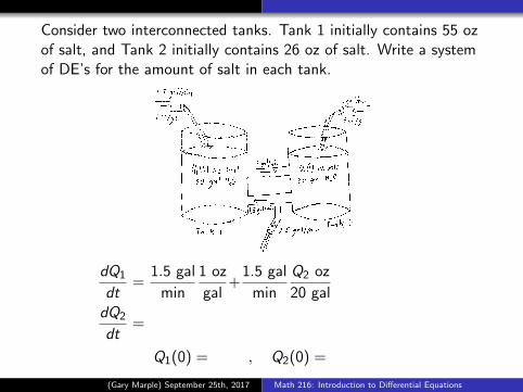
In our example, the right-hand side of the DE only involved thedependent variables Q1 and Q2. Such a system is calledautonomous, just like it was when we had individual DE’s.Another way to visualize solutions of 2× 2 autonomous systems isto consider plots with Q1 on the x-axis and Q2 on the y -axis. Thetwo dependent variables Q1 and Q2 are sometimes referred to asstate variables since the state of the system at any time dependson their values. In addition, the Q1Q2-plane is sometimes referredto as state space, the state plane, or the phase plane. Thereare two common plots in state space. The first one, called avector field, is similar to a slope field, except each line segment isa normalized vector (an arrow) pointing in the direction of thevector 〈dQ1/dt, dQ2/dt〉, the slope of which can be easilycomputed using the chain rule. That is,
dQ2
dQ1
dQ1
dt=
dQ2
dt.
The second plot, called a phase portrait, is the 2-dimensionalversion of a phase line.
(Gary Marple) September 25th, 2017 Math 216: Introduction to Differential Equations

Vector Field showing Q2 vs Q1
Q2 ↑ Q1 →The solid line corresponds to the solution with initial condition
Q1(0) = 55, Q2(0) = 26.(Gary Marple) September 25th, 2017 Math 216: Introduction to Differential Equations
Phase Portrait showing Q2 vs Q1
(Gary Marple) September 25th, 2017 Math 216: Introduction to Differential Equations

Example
Find the equilibrium solutions of the linear system
q′ = Aq + b,
where
q =
[Q1
Q2
], A =
[−0.1 0.0750.1 −0.2
], b =
[1.53
]Remember that equilibrium solutions are constant solutions.Therefore, we need to set q′ = 0.
0 = Aqeq + b
Aqeq = −b (1)
We now have a linear system of equations. We can write thesystem as an augmented matrix. That is,
(Gary Marple) September 25th, 2017 Math 216: Introduction to Differential Equations

Example
Find the equilibrium solutions of the linear system
q′ = Aq + b,
where
q =
[Q1
Q2
], A =
[−0.1 0.0750.1 −0.2
], b =
[1.53
]Remember that equilibrium solutions are constant solutions.Therefore, we need to set q′ = 0.
0 = Aqeq + b
Aqeq = −b (2)
We now have a linear system of equations. We can write thesystem as an augmented matrix. That is,
(Gary Marple) September 25th, 2017 Math 216: Introduction to Differential Equations

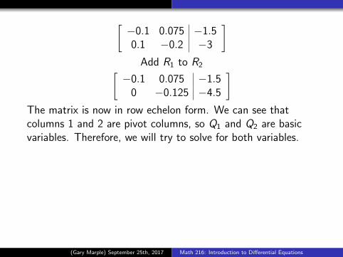
[−0.1 0.075 −1.50.1 −0.2 −3
]Add R1 to R2[
−0.1 0.075 −1.50 −0.125 −4.5
]The matrix is now in row echelon form. We can see thatcolumns 1 and 2 are pivot columns, so Q1 and Q2 are basicvariables. Therefore, we will try to solve for both variables.Converting back to a linear system gives us
−0.1Q1 + 0.075Q2 = −1.5,
0Q1 − 0.125Q2 = −4.5.
We can use the last equation to solve for Q2. That is,
Q2 = 4.5/0.125 = 36.
(Gary Marple) September 25th, 2017 Math 216: Introduction to Differential Equations

−0.1Q1 + 0.075Q2 = −1.5,
0Q1 − 0.125Q2 = −4.5.
Plugging Q2 = 36 into the first equation and solving for Q1
givesQ1 = (1.5/0.1) + (0.075 · 36)/0.1 = 42.
Therefore,
qeq =
[4236
].
(Gary Marple) September 25th, 2017 Math 216: Introduction to Differential Equations

−0.1Q1 + 0.075Q2 = −1.5,
0Q1 − 0.125Q2 = −4.5.
Plugging Q2 = 36 into the first equation and solving for Q1
givesQ1 = (1.5/0.1) + (0.075 · 36)/0.1 = 42.
Therefore,
qeq =
[4236
].
(Gary Marple) September 25th, 2017 Math 216: Introduction to Differential Equations

−0.1Q1 + 0.075Q2 = −1.5,
0Q1 − 0.125Q2 = −4.5.
Plugging Q2 = 36 into the first equation and solving for Q1
givesQ1 = (1.5/0.1) + (0.075 · 36)/0.1 = 42.
Therefore,
qeq =
[4236
].
(Gary Marple) September 25th, 2017 Math 216: Introduction to Differential Equations

Example
Find the critical points of
x′ = Ax + b,
where
x =
[x1
x2
], A =
[2 34 6
], b =
[12
].
Recall that a critical point is the same thing as an equilibriumsolution. Therefore, we’ll set x′ = 0.
0 = Axeq + b
Axeq = −b
We now have a linear system we can express as an augmentedmatrix.
(Gary Marple) September 25th, 2017 Math 216: Introduction to Differential Equations

[2 3 −14 6 −2
]Add − 2R1 to R2[
2 3 −10 0 0
]The matrix is now in row echelon form. In this case, only thefirst column is a pivot column. Therefore, x1 is a basic variableand x2 is a free variable. We’ll start by setting x2 equal to aparameter. That is,
x2 = c .
We can write the row reduced matrix as a linear system. Thatis,
2x1 + 3x2 = −1,
0x1 + 0x2 = 0.
(Gary Marple) September 25th, 2017 Math 216: Introduction to Differential Equations

2x1 + 3x2 = −1,
0x1 + 0x2 = 0
If we look at the first equation, plug c in for x2, and solve forx1, we get
x1 = −1
2− 3
2c .
Therefore,
xeq =
[x1
x2
]=
[−1
2− 3
2c
c
]=
[−1/2
0
]+ c
[−3/2
1
].
In other words, every point on a line in the x1x2-plane is acritical point. Such a situation arises because the two DE’s areexactly the same, just off by a constant.
(Gary Marple) September 25th, 2017 Math 216: Introduction to Differential Equations

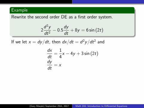
Example
Rewrite the second order DE as a first order system.
2d2y
dt2− 0.5
dy
dt+ 8y = 6 sin (2t)
If we let x = dy/dt, then dx/dt = d2y/dt2 and
dx
dt=
1
4x − 4y + 3 sin (2t)
dy
dt= x
We can express this system of DE’s in the formx′ = Ax + b(t). That is,
d
dt
[xy
]=
[1/4 −4
1 0
] [xy
]+
[3 sin (2t)
0
].
(Gary Marple) September 25th, 2017 Math 216: Introduction to Differential Equations
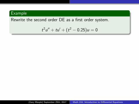
Example
Rewrite the second order DE as a first order system.
t2u′′ + tu′ + (t2 − 0.25)u = 0
If we let v = du/dt. Then, dv/dt = d2u/dt2 and
u′ = v
v ′ = −1
tv − t2 − 0.25
t2u
We can express the system in the form u′ = A(t)u. That is,
d
dt
[uv
]=
[0 1
(0.25− t2)/t2 −1/t
] [uv
].
(Gary Marple) September 25th, 2017 Math 216: Introduction to Differential Equations

Theorem: Existence and Uniqueness of Solutions
Let each of the functions p11, . . . , p22, g1, and g2 becontinuous on an open interval I = α < t < β. Let t0 be anypoint in I , and let x0 and y0 be any given numbers. Then,there exists a unique solution to the IVP
dx
dt= P(t)x + g(t), x(t0) =
[x0
y0
],
where
x =
[xy
], P(t) =
[p11(t) p12(t)p21(t) p22(t)
], g(t) =
[g1(t)g2(t)
].
Furthermore, the solution exists throughout the interval I .
(Gary Marple) September 25th, 2017 Math 216: Introduction to Differential Equations

Example
Transform the given IVP into an IVP with two first orderequations. Then write the system in matrix form.
tu′′ + u′ + tu = 0, u(1) = 1, u′(1) = 0
(Gary Marple) September 25th, 2017 Math 216: Introduction to Differential Equations

(Gary Marple) September 25th, 2017 Math 216: Introduction to Differential Equations

Example
Find the critical points of the system of DE’s.
x ′ = −x + y + 1, y ′ = x + y − 3
(Gary Marple) September 25th, 2017 Math 216: Introduction to Differential Equations

(Gary Marple) September 25th, 2017 Math 216: Introduction to Differential Equations