Embed Size (px)
Citation preview

SECTION 3.8 Newton’s Method 229
Section 3.8 Newton’s Method
• Approximate a zero of a function using Newton’s Method.
Newton’s Method
In this section you will study a technique for approximating the real zeros of afunction. The technique is called and it uses tangent lines toapproximate the graph of the function near its -intercepts.
To see how Newton’s Method works, consider a function that is continuous onthe interval and differentiable on the interval If and differ insign, then, by the Intermediate Value Theorem, must have at least one zero in theinterval Suppose you estimate this zero to occur at
First estimate
as shown in Figure 3.60(a). Newton’s Method is based on the assumption that thegraph of and the tangent line at both cross the -axis at the samepoint. Because you can easily calculate the -intercept for this tangent line, you canuse it as a second (and, usually, better) estimate for the zero of The tangent linepasses through the point with a slope of In point-slope form, theequation of the tangent line is therefore
Letting and solving for produces
So, from the initial estimate you obtain a new estimate
Second estimate [see Figure 3.60(b)]
You can improve on and calculate yet a third estimate
Third estimate
Repeated application of this process is called Newton’s Method.
x3 � x2 �f�x2�f��x2�
.
x2
x2 � x1 �f�x1�f��x1�
.
x1
x � x1 �f�x1�f��x1�
.
xy � 0
y � f��x1��x � x1� � f�x1�. y � f�x1� � f��x1��x � x1�
f��x1�.�x1, f�x1��f.
xaboutx�x1, f�x1��f
x � x1
�a, b�.f
f�b�f�a��a, b�.�a, b�f
xMethod,Newton's
xa
c
Tangent line
bx1 x3
x2
(x1, f(x1))
y
(a)
xa cb
Tangent line
x1 x2
(x1, f(x1))
y
(b)The -intercept of the tangent line approxi-mates the zero ofFigure 3.60
f.x
NEWTON’S METHOD
Isaac Newton first described the method forapproximating the real zeros of a functionin his text Method of Fluxions. Althoughthe book was written in 1671, it was notpublished until 1736. Meanwhile, in 1690,Joseph Raphson (1648–1715) published apaper describing a method for approximatingthe real zeros of a function that was verysimilar to Newton’s. For this reason, themethod is often referred to as the Newton-Raphson method.
Newton’s Method for Approximating the Zeros of a Function
Let where is differentiable on an open interval containing Then,to approximate use the following steps.
1. Make an initial estimate that is close to (A graph is helpful.)
2. Determine a new approximation
3. If is within the desired accuracy, let serve as the final approx-imation. Otherwise, return to Step 2 and calculate a new approximation.
Each successive application of this procedure is called an iteration.
xn�1�xn � xn�1�
xn�1 � xn �f �xn�f��xn�
.
c.x1
c,c.ff�c� � 0,
332460_0308.qxd 11/1/04 3:17 PM Page 229

230 CHAPTER 3 Applications of Differentiation
EXAMPLE 1 Using Newton’s Method
Calculate three iterations of Newton’s Method to approximate a zero ofUse as the initial guess.
Solution Because you have and the iterative process isgiven by the formula
The calculations for three iterations are shown in the table.
Of course, in this case you know that the two zeros of the function are To sixdecimal places, So, after only three iterations of Newton’s Method,you have obtained an approximation that is within 0.000002 of an actual root. The firstiteration of this process is shown in Figure 3.61.
EXAMPLE 2 Using Newton’s Method
Use Newton’s Method to approximate the zeros of
Continue the iterations until two successive approximations differ by less than 0.0001.
Solution Begin by sketching a graph of as shown in Figure 3.62. From the graph,you can observe that the function has only one zero, which occurs near Next, differentiate and form the iterative formula
The calculations are shown in the table.
Because two successive approximations differ by less than the required 0.0001, youcan estimate the zero of to be �1.23375.f
xn�1 � xn �f �xn�f��xn�
� xn �2xn
3 � xn2 � xn � 1
6xn2 � 2xn � 1
.
fx � �1.2.
f,
f�x� � 2x3 � x2 � x � 1.
�2 � 1.414214.±�2.
xn�1 � xn �f �xn�f��xn�
� xn �xn
2 � 22xn
.
f��x� � 2x,f�x� � x2 � 2,
x1 � 1x2 � 2.f�x� �
−1
xx2 = 1.5
x1 = 1
f(x) = x2 − 2
y
x−2 −1
1
2f(x) = 2x3 + x2 − x + 1
y
The first iteration of Newton’s MethodFigure 3.61
After three iterations of Newton’s Method,the zero of is approximated to the desiredaccuracy.Figure 3.62
f
NOTE For many functions, just afew iterations of Newton’s Method willproduce approximations having verysmall errors, as shown in Example 1.
1 1.000000 2.000000 1.500000
2 1.500000 0.250000 3.000000 0.083333 1.416667
3 1.416667 0.006945 2.833334 0.002451 1.414216
4 1.414216
�0.500000�1.000000
xn �f�xn�f��xn�
f�xn�f��xn�f��xn�f�xn�xnn
1 0.18400 5.24000 0.03511
2 5.68276
3 0.00001 5.66533 0.00000
4 �1.23375
�1.23375�1.23375
�1.23375�0.00136�0.00771�1.23511
�1.23511�1.20000
xn �f�xn�f��xn�
f�xn�f��xn�f��xn�f�xn�xnn
332460_0308.qxd 11/1/04 3:17 PM Page 230
SECTION 3.8 Newton’s Method 231
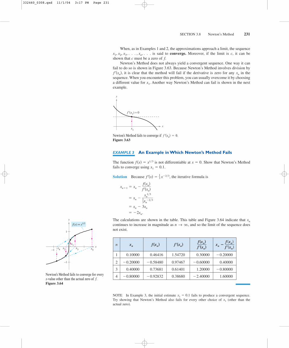
When, as in Examples 1 and 2, the approximations approach a limit, the sequenceis said to Moreover, if the limit is it can be
shown that must be a zero of Newton’s Method does not always yield a convergent sequence. One way it can
fail to do so is shown in Figure 3.63. Because Newton’s Method involves division byit is clear that the method will fail if the derivative is zero for any in the
sequence. When you encounter this problem, you can usually overcome it by choosinga different value for Another way Newton’s Method can fail is shown in the nextexample.
EXAMPLE 3 An Example in Which Newton’s Method Fails
The function is not differentiable at Show that Newton’s Methodfails to converge using
Solution Because the iterative formula is
The calculations are shown in the table. This table and Figure 3.64 indicate that continues to increase in magnitude as and so the limit of the sequence doesnot exist.
NOTE In Example 3, the initial estimate fails to produce a convergent sequence. Try showing that Newton’s Method also fails for every other choice of (other than the actual zero).
x1
x1 � 0.1
n → �,xn
� �2xn.
� xn � 3xn
� xn �xn
13
13xn
�23
xn�1 � xn �f �xn�f��xn�
f��x� �13 x
�23,
x1 � 0.1.x � 0.f �x� � x13
x1.
xnf��xn�,
f.cc,converge.x1, x2, x3, . . . , xn, . . .
1 0.10000 0.46416 1.54720 0.30000
2 0.97467 0.40000
3 0.40000 0.73681 0.61401 1.20000
4 0.38680 1.60000�2.40000�0.92832�0.80000
�0.80000
�0.60000�0.58480�0.20000
�0.20000
xn �f�xn�f��xn�
f�xn�f��xn�f��xn�f�xn�xnn
xx1
f ′(x1) = 0
y
Newton’s Method fails to converge ifFigure 3.63
f��xn� � 0.
x
−1
−1
1
x1x2 x3 x5
x4
f(x) = x1/3
y
Newton’s Method fails to converge for every-value other than the actual zero of
Figure 3.64f.x
332460_0308.qxd 11/1/04 3:17 PM Page 231

232 CHAPTER 3 Applications of Differentiation
It can be shown that a condition sufficient to produce convergence of Newton’sMethod to a zero of is that
Condition for convergence
on an open interval containing the zero. For instance, in Example 1 this test wouldyield and
Example 1
On the interval this quantity is less than 1 and therefore the convergence ofNewton’s Method is guaranteed. On the other hand, in Example 3, you have
and
Example 3
which is not less than 1 for any value of so you cannot conclude that Newton’sMethod will converge.
Algebraic Solutions of Polynomial Equations
The zeros of some functions, such as
can be found by simple algebraic techniques, such as factoring. The zeros of otherfunctions, such as
cannot be found by algebraic methods. This particular function has onlyone real zero, and by using more advanced algebraic techniques you can determine thezero to be
Because the solution is written in terms of square roots and cube roots, it iscalled a
NOTE Try approximating the real zero of and compare your result withthe exact solution shown above.
The determination of radical solutions of a polynomial equation is one of the fun-damental problems of algebra. The earliest such result is the Quadratic Formula,which dates back at least to Babylonian times. The general formula for the zeros of acubic function was developed much later. In the sixteenth century an Italian mathe-matician, Jerome Cardan, published a method for finding radical solutions to cubicand quartic equations. Then, for 300 years, the problem of finding a general quinticformula remained open. Finally, in the nineteenth century, the problem was answeredindependently by two young mathematicians. Niels Henrik Abel, a Norwegian math-ematician, and Evariste Galois, a French mathematician, proved that it is not possibleto solve a fifth- (or higher-) degree polynomial equation by radicals. Ofcourse, you can solve particular fifth-degree equations such as but Abeland Galois were able to show that no general solution exists.radical
x5 � 1 � 0,general
f �x� � x3 � x � 1
radicals.bysolutionexact
x � � 3�3 � �2336
� 3�3 � �2336
.
elementary
f�x� � x3 � x � 1
f�x� � x3 � 2x2 � x � 2
x,
� f�x� f � �x�� f��x��2 � � �x13��29��x�53�
�19��x�43� � � 2
f�x� � x13, f��x� �13x�23, f � �x� � �
29x�53,
�1, 3�,� f�x� f � �x�
� f��x��2 � � ��x2 � 2��2�4x2 � � �12 �
1x2�.
f �x� � x2 � 2, f��x� � 2x, f � �x� � 2,
f
� f�x� f ��x�� f��x��2 � < 1
NIELS HENRIK ABEL (1802–1829)
EVARISTE GALOIS (1811–1832)
Although the lives of both Abel and Galoiswere brief, their work in the fields of analysisand abstract algebra was far-reaching.
The
Gra
nger
Col
lect
ion
The
Gra
nger
Col
lect
ion
332460_0308.qxd 11/1/04 3:17 PM Page 232
SECTION 3.8 Newton’s Method 233
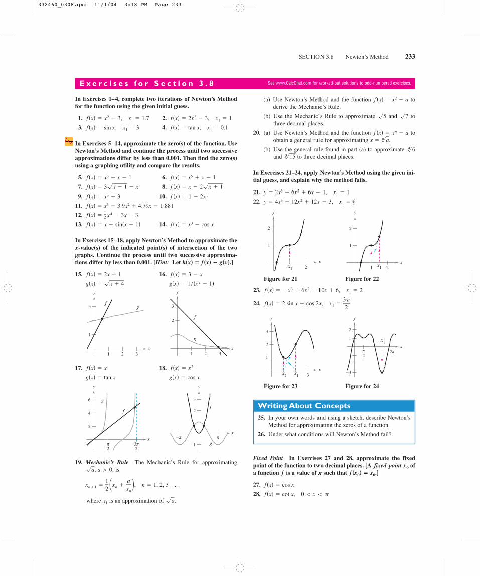
In Exercises 1–4, complete two iterations of Newton’s Methodfor the function using the given initial guess.
1. 2.
3. 4.
In Exercises 5–14, approximate the zero(s) of the function. UseNewton’s Method and continue the process until two successiveapproximations differ by less than 0.001. Then find the zero(s)using a graphing utility and compare the results.
5. 6.
7. 8.
9. 10.
11.
12.
13. 14.
In Exercises 15–18, apply Newton’s Method to approximate the-value(s) of the indicated point(s) of intersection of the two
graphs. Continue the process until two successive approxima-tions differ by less than 0.001. [Hint: Let ]
15. 16.
17. 18.
19. Mechanic’s Rule The Mechanic’s Rule for approximatingis
where is an approximation of
(a) Use Newton’s Method and the function toderive the Mechanic’s Rule.
(b) Use the Mechanic’s Rule to approximate and tothree decimal places.
20. (a) Use Newton’s Method and the function toobtain a general rule for approximating
(b) Use the general rule found in part (a) to approximate and to three decimal places.
In Exercises 21–24, apply Newton’s Method using the given ini-tial guess, and explain why the method fails.
21.
22.
Figure for 21 Figure for 22
23.
24.
Figure for 23 Figure for 24
Fixed Point In Exercises 27 and 28, approximate the fixedpoint of the function to two decimal places. A ofa function is a value of such that
27.
28. 0 < x < �f �x) � cot x,
f �x� � cos x
f �x0� � x0.]xfx0pointfixed[
x
1
2
−3
x1
2π π2
y
x
1
3
2
3x2 x1
y
x1 �3�
2f �x� � 2 sin x � cos 2x,
x1 � 2f �x� � �x3 � 6x2 � 10x � 6,
x
1
1 x1 2
2
y
x
1
x1 2
2
y
x1 �32y � 4x3 � 12x2 � 12x � 3,
x1 � 1y � 2x3 � 6x2 � 6x � 1,
3�15
4�6
x � n�a.f �x� � xn � a
�7�5
f �x� � x2 � a
�a.x1
n � 1, 2, 3 . . .xn�1 �12 xn �
axn�,
a > 0,�a,
x
2
3
f
g−1
π π−
y
x
6
4
2
f
g
π2
π23
y
g�x� � cos xg�x� � tan x
f �x� � x2f �x� � x
x1 2
3
2
3
f
g
y
x
1
1 2
3
3
fg
y
g�x� � 1�x2 � 1�g�x� � �x � 4
f �x� � 3 � xf �x� � 2x � 1
h�x� � f �x� � g�x�.
x
f �x� � x3 � cos xf �x� � x � sin�x � 1�f �x� �
12 x 4 � 3x � 3
f �x� � x3 � 3.9x2 � 4.79x � 1.881
f �x� � 1 � 2x3f �x� � x3 � 3
f �x� � x � 2�x � 1f �x� � 3�x � 1 � x
f �x� � x5 � x � 1f �x� � x3 � x � 1
x1 � 0.1f �x� � tan x,x1 � 3f �x� � sin x,
x1 � 1f �x� � 2x2 � 3,x1 � 1.7f �x� � x2 � 3,
E x e r c i s e s f o r S e c t i o n 3 . 8 See www.CalcChat.com for worked-out solutions to odd-numbered exercises.
Writing About Concepts25. In your own words and using a sketch, describe Newton’s
Method for approximating the zeros of a function.
26. Under what conditions will Newton’s Method fail?
332460_0308.qxd 11/1/04 3:18 PM Page 233

234 CHAPTER 3 Applications of Differentiation
29. Writing Consider the function
(a) Use a graphing utility to graph
(b) Use Newton’s Method with as an initial guess.
(c) Repeat part (b) using as an initial guess and observethat the result is different.
(d) To understand why the results in parts (b) and (c) aredifferent, sketch the tangent lines to the graph of at the
points and Find the -intercept of each tan-gent line and compare the intercepts with the first iteration ofNewton’s Method using the respective initial guesses.
(e) Write a short paragraph summarizing how Newton’sMethod works. Use the results of this exercise to describewhy it is important to select the initial guess carefully.
30. Writing Repeat the steps in Exercise 29 for the functionwith initial guesses of and
31. Use Newton’s Method to show that the equationcan be used to approximate if is an
initial guess of the reciprocal of Note that this method ofapproximating reciprocals uses only the operations of multipli-cation and subtraction. [Hint: Consider ]
32. Use the result of Exercise 31 to approximate (a) and (b) tothree decimal places.
In Exercises 33 and 34, approximate the critical number of onthe interval Sketch the graph of labeling any extrema.
33. 34.
In Exercises 35–38, some typical problems from the previoussections of this chapter are given. In each case, use Newton’sMethod to approximate the solution.
35. Minimum Distance Find the point on the graph ofthat is closest to the point
36. Minimum Distance Find the point on the graph of that is closest to the point
37. Minimum Time You are in a boat 2 miles from the nearestpoint on the coast (see figure). You are to go to a point whichis 3 miles down the coast and 1 mile inland. You can row at3 miles per hour and walk at 4 miles per hour. Toward whatpoint on the coast should you row in order to reach in theleast time?
38. Medicine The concentration of a chemical in the blood-stream hours after injection into muscle tissue is given by
When is the concentration greatest?
39. Advertising Costs A company that produces portable CDplayers estimates that the profit for selling a particular model is
where is the profit in dollars and is the advertising expensein 10,000s of dollars (see figure). According to this model, findthe smaller of two advertising amounts that yield a profit of$2,500,000.
Figure for 39 Figure for 40
40. Engine Power The torque produced by a compact automobileengine is approximated by the model
where is the torque in foot-pounds and is the engine speed inthousands of revolutions per minute (see figure). Approximatethe two engine speeds that yield a torque of 170 foot-pounds.
True or False? In Exercises 41–44, determine whether thestatement is true or false. If it is false, explain why or give anexample that shows it is false.
41. The zeros of coincide with the zeros of
42. If the coefficients of a polynomial function are all positive, thenthe polynomial has no positive zeros.
43. If is a cubic polynomial such that is never zero, thenany initial guess will force Newton’s Method to converge to thezero of
44. The roots of coincide with the roots of
45. Tangent Lines The graph of has infinitelymany tangent lines that pass through the origin. Use Newton’sMethod to approximate the slope of the tangent line having thegreatest slope to three decimal places.
46. Consider the function
(a) Use a graphing utility to determine the number of zerosof
(b) Use Newton’s Method with an initial estimate of toapproximate the zero of to four decimal places.
(c) Repeat part (b) using initial estimates of and
(d) Discuss the results of parts (b) and (c). What can youconclude?
x1 � 100.x1 � 10
fx1 � 2
f.
f �x� � 2x3 � 20x2 � 12x � 24.
f �x� � �sin x
f �x� � 0.�f �x� � 0
f.
f��x�f �x�
p�x�.f �x� � p�x�q�x�
T
xT
1 ≤ x ≤ 5T � 0.808x3 � 17.974x2 � 71.248x � 110.843,
x120130140150160170180190
1 2 3 4 5
Engine speed(in thousands of rpm)
Tor
que
(in
ft-
lbs)
T
x
2,000,000
3,000,000
1,000,000
10 30 50
Advertising expense(in 10,000s of dollars)
Prof
it (i
n do
llars
)
P
P
xP
0 ≤ x ≤ 60P � �76x3 � 4830x2 � 320,000,
C � �3t2 � t��50 � t3�.t
C
Q
2 mi
x 3 − x
3 mi
1 mi
Q
Q,
�4, �3�.f �x� � x2
�1, 0�.f �x� � 4 � x2
f �x� � x sin xf �x� � x cos x
f,�0, ��.f
111
13
f �x� � �1x� � a.
a.x11axn�1 � xn�2 � axn�
x1 � 3.x1 � 1.8f �x� � sin x
x�14, f �1
4��.�1, f �1��f
x1 �14
x1 � 1
f.
f �x� � x3 � 3x2 � 3.
332460_0308.qxd 11/1/04 3:18 PM Page 234