Embed Size (px)
Citation preview
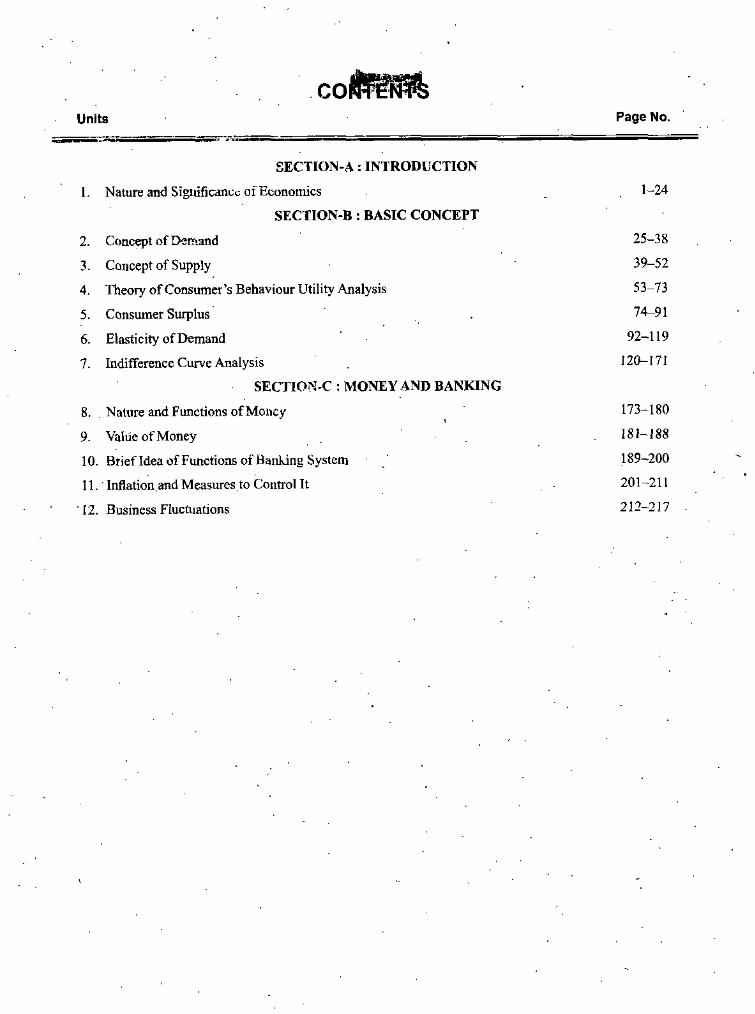
Page No.Units
SECTION-A: INTRODUCTION1-241. Nature and Significanec ofEconomics
SECTION-B : BASIC CONCEPT25-382. Concept of Demand
3. Concept of Supply4. Theory of Consumer’s Behaviour Utility Analysis
5. Consumer Surplus6. Elasticity of Demand
7. Indifference Curve Analysis
39-5253-7374-91
92-119120-171
SECTION C : MONEY AND BANKING173-1808. Nature and Functions of Money
9. Value of Money10. Brief Idea of Functions of Banking System11. Infiation.and Measures to Control It
■ 12. Business Fluctuations
181-188189-200201-211212-217
SYLLABUS
PRINCIPLE OF ECONOMICS
SECTION A
Introduction
Nature and significance of economics,- meaning of science, engineering & technology and their relationship with economic development.
SECTION B
Basic Concepts
The concepts of demand and supply, elasticity of demand and supply, indifference, curve, analysis, price effect, income effect and substitution effect.
SECTION C
Money'& Banking
Function of money, value of money, inflation and measure to control its brief data of function of banking system.
Nature and Significance of EconomicsSecHonr-A : INTRODUCTION
UNIT 1 NATURE AND SIGNIFICANCE
OF ECONOMICS NOTES
★ STRUCTURE ★□ Introduction to Economics
□ Definition to Economics
□ Scope of Economics
□ Business Economics
□ Economic Laws
Q Significance of Economics
Q Central Problems of an Economy
□ Science, Engineering, Technology and Economic Development
INTRODUCTION TO ECONOMICSThe term ‘Economics’ has been derived from two Greek words ‘OIKOU’ and ‘NOMOS’ which, taken together, mean the ruJe or Jaw of the household. At the initial stage of development of human civilisation, economics was confined to the efficient financial management of households. It dealt with the way in which a household could make the best and most efficient use of its limited resources (income) to satisfy its unlimited wants.Later, with the growth and advancement of human civilisation, the concept of efficient financial management of households was carried over to the society and nation as a whole. Wants and needs of every society are unlimited while the resources available with society to satisfy these wants and needs are limited and these limited resources too have alternative uses. Therefore, the .society has to decide the goods and services to be produced with these resources and also the quantity in which these goods and services should be produced so that maximum possible wants of society may be satisfied- Jn other words, the society has to decide how to make the best and most efficient use of available resources.Modern view of economics is not confined only to the allocation of resources but is also concerned with the development of these resources. Though the .wants and needs of every economy have growth manyfolds; population and labour force have increased; sources and techniques of production have improved; infrastructural facilities have improved; facilities of research and development have developed; new natural resources have been explored; both the physical and human resources have grown: and production capacity of modern economies has grown termendously, yet the gi'owth in.production and income has not been smooth. Therefore, economics has to explore and exploit the available
■ resources of economic growth and to employ them for the economic growth of the country. It has also to ensure that the available resources are efficiently utilised for the economic growth and welfare of country. Economics is also
Self-Instructional Material 1
hiduslriul Economy and (Principles of Management
concerned with the increase in productive capacity of scarce resources and the rate of growth of economic development.Kvery economy of today is a complex economy. Several economic problems ^ arise in every economy. Economics is to analyse the causes of these problen-.s and to suggest a number of alternative courses which may help in tadOing these problems.NOTES
DEFINITION OF ECONOMICSIt is nece.ssajy to define the subject which we want to study. Definition of a subject facilitates the understanding of its meaning, nature, characteristics and
. limitations. Therefore, it is necessary to begin the study of economics with its definition.But it is difficult to provide an universally accepted definition of economics because the economists are divided on the question of definition of economics. J.N. Keynes remarked, "Political economy is said to have been strangled itself with definitions.” Mrs. Barabcra Wooten has said, "where six economists are gathered, there are seven definitions.”Though the dispute of definition of economics has not yet come to an end, even an analytical study of all the available definitions is necessary to arrive at a- conclusion. Available definitions of economics can be divided into four parts.. I—Wealth Definitions, .Ill—Scarcity Definitions,
II—Welfare DefinitionsIV—Growth Definitions
Wealth DefinitionsEarly clas.sical economists defined economics as the science of wealth. Adam Smith. J.B. Say, F.A. Walker and other contemporary economists of fSth and early 19th centuries are the economists who defined economics as that part of
• knowledge which is related with wealth. According to them.:"Political Economy is a study of the nature and causes of the wealth
—Adam Smith1-
of nations.”.2. "Economics is the science which trea.ts of wealth.”3. "Economics is that body of knowledge which relates to wealth-”
—J.B. Say
—FA. Walker
Salient Features of Wealth DefinitionsImportant features of wealth definitions may be summarised as fcilows :
1. Central point of the subject matter of economics is wealth.2. Wealth occupies more important place than man.3. Wealth is the only base of human pleasure.4. An ordinary man is au economic nian who performs economic activities
motivated by his 'self only,
o. Individual prosperity adds to national wealth and prosperit}’.
Criticisms of Wealth DefinitionsWealth definitions have been sharply criticised on following grounds ;
2 .S-.-lf-lnstriictinnof Material
Wealth has bee» more emphasised than man. These definitions have confined economics to ‘gespel of marnon’, ‘science of bread and butier', 'a dismal science’.These definitions imagined an 'economic man.' According to these economists, wealth is the only motivating force for all human activities. But this is wrong. A man is motivated by social feelings also, apart from wealth.These definitions use the term 'wealih' in a narrow sense. According to these definitions, wealth includes only material goods. The fact is that wealth means ail the goods and sendees that have utility, .scarcity and transferability.
Nature and Significitntc nf Economics
1.
2,
NOTES
3.
Welfare DefinitionsAlfred Marshall was the first economist to set at rest the criticisms of wealth definitions. He emphasised that man is not for wealth but wealth is for man. The view of Prof.Marshall was supported by Prof. Pigou, Cannon and Clark, etc. According to him :“Economics is a siudy of mankind is the. ordinary business of life. It e.vamines that part of social action which is most closely connected with the attainment and with the use of material requisites of wellbeing."
On the basis of above'definition, it can be concluded that according to Prof. Marshall economics is the study of material welfare of mankind.
—Marshall
Salient Features of Welfare Definitions1. Economics is the Study of Ordinary Business of Life. Economics is
the study of ordinary business of life. Ordinary business of life relates to those activities which are performed by an ordinary man for earning and using his income.
2. Economics is a Social Science. Economics is a social science. Itstudies the economic problems of those individuals only who live in a well organised society.
3. Economics Studies only the Economic Activities. Economics studies only those economic activities that promote material welfare of human being. Thus, non-economic activities are not included in the scope of
■ economics.4. Dominance of Man. Welfare definitions have emphasised upon the
importance of man. According to Prof. Marshall, man is not for wealth, wealth is for man. According to him, wealth is only a means
. and not an end..End is human welfare.5. Economics is Both a Science and an Art. According to Prof. Marshall,
economics is a science as well as an art. Economics is a positive .science because it studies the principles of human life in a systematic manner. It is a normative science also because it attempts at attaining material welfare. It is an art alsu because it develops the methods of attaining human v^elfare.
Criticisms of Welfare Definitions
For a long time, welfare definitions of economics were accepted without criticisms and it was being felt that the problem of defining economics has come to an
Self-Instructional Material ?
Industrial Economy and PrineipJes of Management end. But this situation could not continue for ever. In 1932, Prof. Lionel
Robbins broke new grounds in defining economics in his book ‘The Nature • and Significance of Economic Science’. Some of the important criticisms of
welfare definitions are as follows ■.1. The Classification of Human Activities into Economic and Non-Econnmic
is Impracticable. Welfare definitions classify human activities into economic and non-economic- Prof. Robbins was of the view that .such distinction of human activities is illusory and impracticable because all human activities have an economic aspect.
2. The Classification of Material and Immaterial Welfare is Impracticable. According to welfare definitions, economics is the science of material welfare. Prof. Robbins criticised this view on .the ground that it is wrong to differentiate between material and immaterial welfare. He was of the view that human welfare is associated with both the material and immaterial means of welfare.
3. Economics is a Human Science, and not only a Social Science. According to Prof. Marshall, economics is only a'social science but the critics are of the view that it is a human science also not only a social science. Many laws of economics apply on those people also who do not live in well-organised society.
4. Illusory Meaning of Ordinary Business of Life. According to Prof. Robbins, human activities cannot be classified as ordinary and extraordinary. Secondly, the study of economics cannot be confined to ordinary business of the life only because the activities of extraordinary business of life such as war, monopoly, imperfect competition etc., are essentially the subject matter of economics.
5. Welfare Definitions make Economies a Normative Science. Prof. Robbins criticised welfare definitions on the ground that these definitions have made economics a normative science. He believed that it is not proper to relate economics with welfare. He remarked, “Whatever economics is concerned with, it is not concerned with the causes of material welfare as such.” According to him, economics is a positive science.
6. Narrow Scope of Economics. Prof. Robbins criticised welfare definitions on the ground that these definitions have narrowed the scope of economics by excluding non-economic, immateJial and unsocial activities:
NOTES
Scarcity DefinitionsProf. Lionel Robbins not only criticised welfare definitions but also proceeded to give a new definition to economics. He gave his definition in his book Nature and Significance of Economic Science' published in 1932. According to him, “Economics.is a science which studies human behaviour as a relationship ends and scarce means which have alternative uses.”
The views of Prof. Robbins were fully supported by many famous economists including Eric Roll, Cairncross, Friedman and Stigler etc.
Salient Features of Scarcity DelHnitions1. Human Wants are Unlimited. Human wants are unlimited and-the
intensity of all the wants is different. Though a particular want can be satisfied at a particular time but as soon as' one want is satisified, another crops up. Thus, a man is always surrounded by his wants.\ Self-Instructional Material
Salure and Significance of Economics
He can never satisfy alJ.of his wants. Therefore, the need arises to choose between more and less urgent wants. It gives rise to the economic problems.
2. 'Means to Satisfy Human Wants are Scorce. The resources availablewith every person are limited, therefore, he is to choose rationally between limited resources and unlimited wants. A man has to decide which want to satisfy and which to leave. Then he is to decide which want should be satisfied first and which after some time. He has to see how best he can use his limited resources.
3. Scarce Resources Have Alternative Uses. The problem of unlimited wants and scarce resources becomes more serious becasue of the fact that scarce resources have alternative uses. These resources can be put to several alternative uses. If we want to use the given resources for a particular use, all other alternative uses of these resources will have to be given up. It gives rise to the problem of choice and a man has to choose the beat possible uses of his resource's.
4. Economics is a Human Science. According to Prof. Robbins, economics is a human science. It studies the activities of all the persons, whether they are or they are not a part of society.
5. Economics is a Positive Science. According to Prof. Robbins, economics is a positive science. According to him, economics is the science of resources and is not concerned with ends.
6. Analytical. Scarcity definitions of economics are analytical. According to these definitions, economics studies the aspects related witli choice and human activities. It is not confined to the study of some particular types of activities.
NOTES
Criticisms of Scarcity. DefinitionsScarcity definitions have been criticised by many economists. Important criticisms of these definitions are as under :
1. Economics is not only a Positive Science. According to Prof. Robbins, economics is a positive science. But many economists like, Souter, Parson and Macfic etc. regard economics-as a positive and normative science both.
2. Economics cannot be Neutral between Ends. According to Prof. Robbins, economics is neutral between ends but it is not a real implication. Economics is concerned with human behaviour and therefore, it cannot be neutral between ends.
3. Economics without the Concept of Welfare and Measuring rod of Money.■ The definition of Prof. Robbins has been criticised on the groundthat it establishes economics without the concept of welfare and measuring rod of money. The reality is that ail the human activities are motivated to get welfare. Similarly, the science of economics is incomplete without measuring rod of money.
4. Economics is not only a Value Theory. According to Prof. Robbins, economics is the study of allocation of resources. Thus, according to
' Robbins, economics has been confined only to a theory of value but the scope of economics is much wider than the allocation of resources and price theory. It should include the study of national income and employment also.
Self-Instructional Material S
Industrial Economy and Principles of Management
5. Economics is not only Micro Analysis. According to Prof. Robbins, economics is concerned with individual behaviour of satisfying uulimitied wants with scarce resources having alternative uses. Thus, economics has been confined to micro analysis only. But it is not, true.Robbins ^o:. RcstriciJu and Widened inc Scope of Economics. Prof.
■ as the scope of econo.'-ncr, by gi'ing his riefinition ' ,in terms oi the pronlem of scarcity and choice. The problem of choice applies on all the human activities but all these cannot be included in the scope of economics.Economics is nut only a Science but an Art also. According to Prof. Robbins, economics is only a science which aims at formulating economic principles only But this is not a realitj'. Those principles should be implemented properly for the welfare of human beings.Thus, economics is an art also.Robbins has Imagined a Very Rational Man. According to the definition of Prof. Robbins, a man allocated his scarce resources most efficiently so that he may satisfy most of his wants. Thus, Prof. Robbins imagines that a man always behaves rationally But the practical experience of life does not prove this imagination.
6.NOTES
7.
Growth DeHnitionsModern economists define economics in following manner ;"Economics is the study of how man and society choose, with or without the u.se of money, to employ scarce productive resources which could have alternative uses, to produce various commodities over time and distribute them for consumpiK^n now and in the future among various people and groups of society."
—Prof. SamuclsonThus, modern economists regard economics much more broadly. According to them, economics is coiicerned with suggesting the ways and means in which the available resources can be allocated rationally and in which, these resources can be further increased t that maximum satisfaction of wants may be assured.
Comparison between the Definitions of Marshall and RobbinsWhich of the definitions of Prof. Marshall and Prof. Robbins is better—is an alive controversy- Both the definitions are based upon different views. A comparison • of these definitions reveals the following facts :
The definition of Prof. Robbins is more scientific than that of Prof. Marshall because it provides a scientific base to the study of economics in the form of scarcity and choice.The definition cf Prof. Robbins is m.ore logical than that of Prof. Marshall because it highlights a reality of life that human wants are unlimited and the resources to satisfy these wants are limited, that too with alternative uses.According to Prof. Marshall, economics is only a social science but according to Prof. Robbins, economics is a human science.According to Prof Marshall, economics studies only the economic activities while according to Prof, Robbins, economics studies both the economic and non-economic activities.
1.
2.
3.
4.
6 Self-Instructional Material
■ 5. According to Prof, Marshall, economics aims at increasing humanwelfare while according to Prof. Robbins economics is not concerned with human welfare.
6. According to Prof, Marshall, economics is both the science and art. According lo Prof, Robbins economics is only a positive science arid not an art.
7. The definition of Prof. Marshall is classificatory while the definition of Prof. Robbins is analytical.
Thus, it may be concluded that no definition of these two can be regarded as better. Theoretically, the views of Prof. Robbins are more justified but practically the views of Prof. Marshall are more practical.
Nature and Significance of Economics
NOTES
SCOPE OF ECONOMICSAccording to Stonier and Haugue the subject matter of economics includes the following:
1. Econounc. Thsory. The theoretical part of economics is economic theory. The economic theories and economic tools frames this part. This part is divided inle static dynamic economics. The ether name of his part is ‘Economic Analysis'.
2. Applied Economics. Applied Economics tries to apply the results of aconomic analysis to descriptive economics. There are many examples of Applied Economics such as Industrial Economics. Managerial Economics and Agricultural Economics.
3. Descript've Ecoromics. In descriptive economics actual facts about a particular economic subject for the aim of study. Indian Economics is the example of de.script!ve economics.
BUSINESS ECONOMICS
Meaning of BusinessHuman beings in order to satisfy their needs take up many activities. These activities can be broadly classified as economic and non-economic activities.
< Business is thus a typical economic activity. The dictionary meaning of business ’ is employment, trade, commercial activity or industrial concern. Business is a
\vide term which includes individual and group activities directed toy.-ards the wealth acquisition through exchange of goods and/or seivices. Business includes activities such as farming, mining, manufacturing, banking, trading, ins'urance, transport, construction and warehouse etc. which are taken up with a profit orientation.
Concept of Business EconomicsBusiness Economics was attached different meanings in- accordance with the objectives set.According to one school of thought, business economics was conceived as an activity aimed at profit maximisation- In the early days, the sole objective of business was to earn profit at any cost in prder to accumulate wealth, gain economic.power even at the cost of social justice.
Self-instructional Material 7
Industrial Economy and Principles of Management
This concept has become almost outdated and the modern concept of business economics believes in the fact that business is a long lasting social and economic institution. The main objective of the business economics is to be in businoss. The business economics in order to survive and grow has to make profit along with meeting other societal obligations. Now, the new concept is “Profit through Service". Thus, along with economic objectives of profit maximisation, social responsibilities of business towards various stakeholders like owners, workers, consumers, society and government have gained a considerable importance.
NOTES
Managerial EconomicsManagerial economics can be viewed as an economics applied to problem solving at the firm level. Managerial economics deals v;ith integration of economic theory with business practices for facilitating the decision making planning process by management.Thus, managerial economics provides the link between economics and the decision science disciplines like mathematics,- statistics, operation research, econometrics etc. in decision making.
Macro and Micro EconomicsMacro-economics studies the functioning of the economy as a whole andonicrO economics analyses the behaviour of individual components like industries, firms and households.Micro-economics basically provides answers to the following questions :
(i) What goods should be produced and in what quantity ?{«) Mode of their production (how they are produced)
(Hi) How the goods should be distributed ? .(iv) How efficiently the resources are utilised ?
Thus, Micro-Economics deals with the theory of the firm and behaviour and problems of individuals and firms. It is concerned with pricing theory, demand concepts and theories of market structure. It has a relevance to managerial economics.Macro-Economics is concerned with such economic variables as the aggregates output of an economy, extent to which the resources are employed, the level and determination of national income, balance of payment etc.Macro-economics examines the aggregates and averages of economic variables which included study of money, banking and financial institutions, general price levels, inflation theory of employment, income distribution, monetary and fiscal policies and problems of economic stabilisation.
Nature of Economics : Economics as a Science and as an ArtMeaning of Science. Science is a systematised body of knowledge which establishes relationship between cause and effects. It is a systematic collection, classification and analysis of facts. In the words of Prof. Poincere. “Science is built up of ’ facts as a house is built up of stones, but an accumulation of facts is no more • a science than a heap of stones in a house,” Thus, following are the essentials of science :
(0 A systematic study of facts,
8 Self-Instruetiohal Material
Hi) certain rules and principles,(iii) rules and principles of science are based on causes and effects, and (ty) rules and principles of science are universally applicable.
Nature and Significance of Economics
Is Economics a Science : Arguments in FavourScholars who argue that economics is a science, put the following arguments in favour of their opinion ;
Sy5^emo^^c Study of Facts. Economics involves the systematic collection, classification and analysis of facts. Economic results are measured in terms of money. Therefore, economics can be treated as a science.Use of Economic Laws and Principles. Study of economics involves the use of number of economic laws and principles. Economic facts are analysed on the basis of these laws ahd principles./( Establiskes Relationship Between Causes and Effects. "Economics establishes relationship between the causes and effects of economic events. Such relationship facilitates economic forecastings.Universality of Laws and Principles. Laws and principles of economics are universal- They hold true in almost all the countries at all the times and in all the circumstances.
NOTES
1.
2.
3.
4.
Is Economics a Science : Arguments AgainstSome scholars argue that economics is not a science. They put the following arguments in favour of their opinion ;
Difference in the Opinion of Economists. There is vast difference in the opinion of economists on almost every issue. It is said that where six economists are gathered, there are seven opinions. In view of these differences, economics cannot be a science. This argument can be cancelled on the ground that economics is a social science and not a physical science. Existence of difference of opinion is a healthy sign of the vigour and vitality of a social science.Lack of Universal Lows and Principles. Laws and principles of economics are not universal. They change with a change in circumstances. Due to this reason also, economics cannot be a science. This argument can be cancelled on the ground that the subject matter of economics is ‘Man’ and not '‘Material’. A man, being a rational human being, cannot be subject to a definite law or principles in all circumstances.Lack of Ability to Forecast. Some critics eire of the view that reliable predictions are not possible to be made in economics. Therefore, it cannot be science. This ailment can. be csincelled on the ground that economics studies human behaviour and human behaviour is always dynamic. However, the predictions regarding society and nation
. as a whole, generally hold true.Lack of Reliable Economic Facts and Data. Facts and data used in economics are not complete and reliable. Therefore, it cannot be science. This argument can be cancelled on the ground that it is due to the dynamic nature of economic circumstances. However, this problem can be tackled to a large extent with the use of statistical methods.
1.
2.
3.
4.
Self-Instructional Material 9
Industrial Economy and Principles of Management
Cpnclusion. Above discussion makes it dear that economico is a science. It possesses all the characteristics that a science should possess. However, the laws and principles of economics are not as static and definite as the laws and principles of other sciences like physics and chemistry. It is mainly due to the
■ fact that economics is a social science and subject matter of economics is the study of dynamic human behaviour.Meaning of Art. Art means the systematic branch of knowledge which teaches how .to do a particular work in its best manner. Art i6 the practical application of Scientific principles. Science lays down certain principles while art puts these principles into practical use. According to Dr. Mac Coll, “Arf is just the way of doing or making anything in such a fashion as to bring rhythm in it.” According to J.N, Keynes, “An Art is a system of rales for the attainment of a given end.’
NOTES
Is Economics an Art : Arguments in Favour
The scholars who argue that economics is an art, put the following arguments in favour of their opinion :
1. Helpful in the Solution of Economic Problems. Economics suggests the wdys in which economic problems of a country can be solved in their best manner.
2. Increasing Importance of Applied Economics. Applied economics is gaining more and more importance day by day Economics emphasises upon the adoption of practical policies in place of theoretical laws and principles. It highlights the artistic view of eccuomics.
3- Economic Aspect of Problems. Almost all the problems arising in the woriu 01 today are economic problems in one sense or another. These problems must be analysed from economic point of view also. It also highlights the artistic view of economics.
4. Economics as an Art Does Not Weaken Its Scientific Aspect. Some critics are of the view that as economics is a science, ii- cannot be an art. But it is not true. The fact is that ev.?ry ecience has its art, so the Scicr.ee of Economics has un Art of Economics as well. Science lays dc-wn certain principles while art puts these principles into practical use.
Is Economics an Art : Arguments AgainstSome scholars are of the opinion that economic? is not an art. They put following arguments in favour of their opinion :
1. Difference in the Nature of Economics and Art Nature of both the economics and art are quite different from that of each other. Economics is of scientific nature, therefore, it cannot be art.
2. Economics is to Draw only the Conclu?’on.s nnd Net t' Formulate The Policies. Economics is.helpful in drawing the conclusions only, it does not help in formulating policies. In this form, economics is only a science and not an art.
3. Lack of Pure Economic Problems. No problem of eccaomics is a pure economic prollem. It has some social, political and'leligious aspects also. Therefore, no problem can be solved on pure economic grounds.
t
10 Self-Instructional Material
Conclusion. Above dipcussinn makes it clear that economics is both a science and an art. Subject matter of economics is the study of "human behaviour. Human behaviour ^ves rise to two sets of phenomena, one is the practice of working out that behaviour and other is the theory that helps that practice. Economics i? studied a? a science and nrartised ns an art. Thus, an economist works as a scientist when he studios economics and as an artist when he practices it. In the words of Cossa, "Science requires art. art requires science, each being complementary to other.”
Nature and Significance of Economics
NOTES
Economics as a Positive and Normative ScienceMeaning of Positive Science. Positive science is that branch of science which states the actual situation. Positive science is concerned witii the establishment of relationship between causes and effects of an event. It indicates actual facts and does not give any judgement about them. It only replies ‘what it is’ and not ‘what it should be’. In the words of Prof. Keynes, "A Positive Science may be defined as a body of systematised knowledge concerning what is.”
Economics as a Positive ScienceClassical economists like J.B. Say, Senior and Mill, Robbins, Cairncross, and Bagebot were of the opinion that economics is a positive science. According to them, object of economics is to establi.sh a relationship between the causes and effects of an event and not to suggest the ways to tackle with the event. According to them an economist is supposed only to, narrate the actual facts and not to recommend .dissuade. Ecoiioiiiics is a positive science as follow :
In Consumption. In the field of consumption, many laws of economics establish that it is a positive science such as the Law of Diminishing Marginal Utility, Law of Equi-marginaJ Utility, Consumer’s surplus, Indifference Curve Analysis etc. All of these laws establish relationship between causes -and effects of economic events.In Production. In the field of production, Laws of Returns and Scales to Returns establish relationship between causes and effects of different situations and stages of production.In Exchange. In the field of exchange, law ot Demand and Law of Supply establish economics as a positive science. In addition to this, price under different forms of market is also determined on the basis of principles of positive science.In Distribution. In the field of di.stribution, theories of rent, wages, interest and profit have been developed on the basis of principles of positive science.In Public Finance. In the field of public finance, cannons of public expenditure, cannons of taxation and the cannons of public debt establish that economics is a positive science.
Conclusion. Above discussion makes it clear that economics is a positive science. It narrates actual facts and establishes relationship between causes and effects of economic events. In the words of J.B. Say, “Whatever owe to the public IS to tell them how and why such a fact is the consequence of another. Whether the conclusions be itelcomed or rejected, it is enough that the economist should have demonstrated its causes but he must give no advise. “In the words of Prof. Robbins,” The function of economics consists of exploring and explaining and not advocating and condemning. Economics is neutral between ends.”
1,
2,
3,
4.
5.
Sdf-lnstructional MaIrrinI II
Industrial Economy and Principles of Management Meaning of Normative Science. Normative science is that branch of science
which is related with directing and formulating policies. Main object of normative science is the determination of ideals. It tells us what should be done and what should not be done in given circumstances. In the words of J.N. Keynes, "A normative or regulative science may be defined as a body_of systematised knowledge relating to the criteria of what ought to be.”Economics as a Normative Science. Many economists like Marshall, Pigou, Frazor, Hawtrey, Barbara Wooton etc. were of the opinion that economics is a positive as well as normative science. Mahatma Gandhi, the father of nation, has also described economics as normative science.Argument in Favour. Economics can be described as normative science on the basis of following arguments :
1. Economics only as Positive Science will be Meaningless. If economics is only a positive science and is concerned only with establishing the relationship between causes and effects of economic problems, it will be monotonous and meaningless. It is of no use to analyse economic problems without finding a solution to them.
2. Economics cannot be separated from Human Welfare. Economics is a social science. Subject matter of economics is the study of human behaviour. In this way, it cannot be separated from human welfare.
3. Dynamic Economic Conditions Make Economics Normative. Every economy of the world is a dynamic economy and economic conditions of every economy keep on charging rapidly. It necessitates that appropriate decisions should be taken at appropriate time and this is not possible if economics is only a positive science.
4. Helpful in the Solution of Economic Problems. Several economic problems arise in every economy. These problems can be solved only if economics is taken to be the normative science.
Arguments Against. Scholars who argue that economics is not a normative science, put following arguments in favour of their opinion •.
1. Normative Science is Based on Emotions. Normative Science is based more on emotions than on logic and facts. It weakens the logical aspect of economics. Therefore, economics should not be treated as normative science. •
2. Normative Science Invites Disputes. Normative Science describes what should be done and what should not be done in given circumstances. This is the issue on which the economists can never have unanimous opinion. It invites and gives rise to disputes among economists.
3. Possibility of Causing Confusion. Positive Science is. concerned with ‘what is’ and normative science is concerned with ‘what should be.’ If they are taken together, it may cause confusion among economists.
4. Against the Principle of Division of Labour. It is the time of specialisation and division of labour. Economics should confine itself to the analysis of economic problems. Determination of policies and solution of problems should be left to executive.s and politicians.
Conclusion. Above discussion makes it clear that economics should be treated ^ normative science as well as positive science.
NOTES
12 Self-Instructional Material
Nature and Signipcance of EconomicsECONOMIC LAWS
Meaning and Definition of Economic LawsEvery science has some certain laws and theories. These laws explain the relationship between causes and effects of given events. Economics is also a science and, therefore, it has also some certain laws and theories. These laws and theories are known as economic laws. Economic laws explain relationship between causes and effects of economic events. For example, law of demand is an economic law which explair.a relationship between ‘cause’ (changes in price of a commodity) and ‘effect’ (changes in demand of a commodity). This law explains that the demand of a commodity falls on an increase in its price and increases on a fall in it's price. Economic laws have been defined as follows :
1. "Economic laws are the statements of economic tendencies, or those social laws which relate to branches of conduct in which the strength of motive concerned can be measured by money price.” —Marshall
2., “Economic laws are the statements of uniformities about human behaviour concerning the disposal of scarce means with alternative uses for the achievement of ends that arc nrJimited."
Thus, it may be concluded that economic laws are the statements of regularities of cause and effect arising from the free working of economic forces. Those laws deal with those human activities than can be measured in terms of' money.
NOTES
—Robbins
Characteristics of Economic liawsBased on Human Behaviour. Subject matter of economics is study of human behaviour, therefore, economic laws are based on human behaviour. Due to this reason, these laws are known as Social Laws also.Relative Laws. Economic laws are relative, and not absolute. These laws apply in specific circumstances at specific times and places. Laws applying in a particular area or at a particular time may not hold true in other areas or at other times.Based on certain Assumptions. All economic laws are based on certain assumptions. Since it is not always practical that all of fiiese assumptions hold true simultaneously, some critics are of the view that economic laws are only imaginary and do not hold true in practical life. jDifferent from Natural Laws. Economic laws are based on human behaviour and human behaviour is so various and uncertain that no • law on human behaviour can be as certain and universal as natural law. As a matter of fact, economic laws are only the statements of economic tendencies.
Conclusion. Economic laws are social laws and are based on human behaviour. As human behaviour is dynamic and uncertain, these laws are also dynamic. These laws are not universal like natural and physical laws. In the words of Prof. Waugh, ‘Economic law.s are qualitative statements and not the quantitative- statements; these lavjs iridicate only the direction of change and not the quantity of change.”
1.
2.
3.
4.
Self-Inrtructinna> Matenat 13
Industrial Ecnniiniy and Principles of Motiagement Justification of Economic Laws
There is a great controversy on the quesiion whether economic Jaws are only the theoretical statements or these is any practical utility of these laws. Some economists are of the view that economic laws are very useful in the study of economics while some other economists arc of the view that these laws are only theroretical and have no practical utility. They put following arguments in favour of their opinion :
These laws are relative and hold true only at a particular time and place.These laws are hypothetical and are based on 3 rumber of assumptions. Since these assumptions do not ljuld tiue r.t ul! times and places, iheac; laws also do not hold true at ah uinrs uud places.These laws are based on human behaviour. As human behaviour is always dynamic and uncertain, how these laws can be reliable.These laws are less certain and rigid than natural laws.
Though it is true that there are certain limitations of economic laws, but it does not mean that these laws are only theoreticgl statements and have no practical utility. The fact is that these laws, if studied in the light of certain limitations, highlight many important aspects of human behaviour. These laws are valuable guides in the field of consumption, production, distribution and public finance. Following words of iProf. Marshall are important in this regard, “The laws of economics are to be compared with the laws of tides rather than with the simple and exact law of gravitation’'. Prof. Robbins was very hopeful of the utility of these laws saying, “Economic laws describe inevitable impheuiions. If the data they postulate are given, then the consequences they predict necessarily follow.”
NOTES
(i)
Hi)
(Hi)
(iv)
SIGNIFICANCE OF ECONOMICSEconomics is useful not only to individuals but also to business firms and the society as a whole. Economics provides certain tools which can be used for solving various business problems. Knowledge of economics is useful in almost all spheres of life. It helps a iusicvCioouin ir; hie v<.r:.jui, f-Kisiom with, regard to price, quantity, cost, size etc. It helps a policy makes in formulating appropriate policies for the economy and it even helps a housewife, in budgeting hei finances. However, economics is merely a tool in the band.® of user.s. It does not furnish a body of set principles or readymade .solutions to various problems. It only widens and deepens the understanding of functioning of various forces.
Importance for IndividualsIndividuals often face the problems of scarcity and choice-making. ICnowledge of economic.s is quite helpful here. An individual can read the market forces and take decision about th" time and the rates at which to buy desired products. The concepts of marginal utility, indifference curve, etc, help thedndividuai to maximise his satisfaction with the use of minimum resources.
Importance for Business Firms
Economic laws and theories establish cause and effect relationship -which I true under certain assumptions. The laws of production are particularly helpful
are
14 Sflf-hsstructional Material
to basiness-ar. optimum factor mij. :c the nrc- of resources can be achieved through the use of the law of vuriable proportions.Production is undertaken in anticipation of demand. Economics helps in forecasting demand. It is based on a number of lactors concerning the product and some external forces. It depends on the size of market, the degree of competition, elasticity of demand and the general economic situation, These estimates also help in finding out the- likely return on investment.For making a suitable choice of location for the business, an entrepreneur must know about the availability of raw materials, transport facilities, power and labour. The price situation also influences the demand for the product. The exchange rate has a bearing on the value which will be realised from exports. Indirectly, the general price level and the foreign exchange rate influence the overall economic activity m the country and, therefore, the business prospects of a given product.Economics helps a business manager to analyse the cxtei'iial environment of business. For example, the Government influences business through its fiscal, monetary and industrial policies. A businessman must be aware of these policies and the implications on his business anti -what is happening in other countries because, in the modem era of economic interdependence, business in a country is bound to be affected by conditions in the world as a whole. What is of importance is that businessman should be able to analyse the causes and effects of such forces on his business, r-tr this purpose, the various laws of economics should prove very usefulHowever, economics does not furnish a body of set principles or ready-made solutions to various problems which can be applied to a given situation. It only • widen and depends on one's understanding of the economic forces. Actual application of the laws v/ill depend on the exigencies of each situation. If the mind is trained in economic logic, finding the solution to various economic problems should not be difficult.
Nature and Significance of Economics
NOTES
Importance for the Nation'Economics deals with the laws and principles which govern the functioning of an economy and its various parts. An economy exists because of two basic facts. Firstly, human wants for goods and services are unlimited, and secondly productive resources with which to produce goods and services are scarce. Therefore, an economy has to decide how to use its scarce resources to obtain the maximum possible satisfaction of the members of the society. It is this basic problem of scarcity which gives rise to many of the economic piohleii.;,.The subject-matter of economics has been divided into two parts. Micro- I economics and macro-economics. Micro-economics deals with the analysis of , small individual units of the economy such as individual consumers, firms, industries and markets. On the other hand, macro-economics concerns itself with the analysis of the economy as a whole and .its large aggregates such as total national income, output, employment etc.The problem', of scarcity and choice-mo.Ving can be solved in many ways by an « economy. If it gives the whole charge of the economy to private ownership, we get capitalist economy, to public ownership we get mixed economy. Each type of economy development. With the help of economic principles and laws, the national government can make plans for the effective use of various resources for economic growth of the nation and for raising standard of living of the general public.
Se/f-lnslruclintiri/. Mc'-rhl 15
Industrial Economy and Principles of Management CENTRAL PROBLEMS OF AN ECONOMY
An economic system refers to economic relationships which arise in the community from the organisation or mode of production and distribution. In other words, an economy refers to a-system in which people organise their activities and form institutions whereby the economic resources, namely, land minerals, power, raw materials, labour, capital and other inputs of production, are utilized for satisfying the needs of the people living in the society. The fundamental problem for an economy is to provide answer to the following three fundamental questions : « .
NOTES
(i) What things will be produced ? This in simple- terms means that there must be some method of determining tho goods which are to be produced- The economic system must provide for the determination of the goods to be produeed.
(«) How will things be produced ? A primary function which an economic system must perform is to determine the methods of production. In particular, to what proportions shall the factors of production be combined ? The choice of techniques of production is extremely important for any economic system.
iUi) For whom will things be produced ? Here the basic problem is to determine how to distribute the total product among the population.
These three problems are fundamental and common to all economies and all of them are forever engaged in solving them. Apart from these basic problems, there are tliree other important problems which have been pointed out by Richard G. Lipsey. These are .
(i) How to achieve the level of full employment ?(ii) ffou> to achieve efficiency' in utilisat ion of productive resources and
distribution of what has been produced ?(Hi) How to achieve maximum possible rate of economic growth ?
The above questions would be decided with reference to the nature of economy as to whether it is a capitalist economy, or a socialist economy or a mixed economy. Each type of economic system therefore, in trying to provide adequate answer to the above questions would fix certain goals with reference to the given economic structure and the nature and working of particular factors prevalent in that economic system.Every economic system is supposed to exist primarily to create such condition as to make it easy for human beings to satisfy their wants. However, the exact manner in which the problems like allocation of resources among various alternatives uses, fixation of priced, and direction and determination of input and output will be tackled, would depend upon the particular type of economic system which is adopted by a particular country.
Role of Government/Public PolicyAccording to.Lipsey and Steiner, “Economics develops specific criteria which define the conditions for making the best use of society's resources and employs these criteria a.? guidelines for formulating and evaluating public policy.” The basic problem of a society is the efficient use of scarce resources so that the maximum possible number of wants are satisfied. Every government has to lay down the criteria for efficient use of resources. To be specific; the government has to take decisions in the following problem areas :
16 Self-lnsfuctional Material
Nature and Significance of Economics
(i) Determination of goods to be produced. There'must be some method of determining the kinds and quantities of goods to be produced in the economy. The economic system must also provide for the determination of the standard of goods to be produced by the production units.
lii) Vtilizoiwn of resources. The resources of any economy are limited. So the basic problem is the maximum possible and efficient use of productive resources for the social welfare of the economy.
(t«) Choice of techniques ofproduction. The economic system must determine the techniques of production. What technology should be used to produce a particular product ? Should it be a traditional pairs of bullocks and a plough or produce wheat? In what proportions should the various factors of production be combined?
{iv) Distribution of products. This is an important problem in economies where a section of the society is very poor. The government rnay distribute essential commodities through fair price shops. It may introduce dual pricing in industries so that goods at low prices are made available to the poor. The government ailso interferes in the pattern of income distribution. It levies high rates of direct and indirect taxes on the wealthy persons,
(v) Efficiency of production system. The efficiency of production system in a particular year is the ratio of output to input. Higher the ratio, higher is the efficiency. This index of different years is compared to know whether the efficiency has increased or decreased,
(vi) Growth of economy. The economy should not remain static, it must grow over a period of time if the standard of living of the people is to be raised. The growth of an economy depends upon the exploitation of natural resources, technological advancement and capital fornjation in the country.
NOTES
SCIENCE, ENGINEERING, TECHNOLOGY ASD ECONOivnC DEVELOPMENT
Meaning and Nature of ScienceScience is the systematised body of knowledge pertaining to a particular field of enquiry. Such systematised body of knowledge pertaining to a particular field contains concepts, theories and principles which are universal and true. Science has the following features
(i) Systematised' body of knowledge tii} Scientific methods of observation
[Hi) Tests of validity and predictability (io) Universal application of principles
Whatever field of enquiry fulfills the above criteria is called a science. The important examples of science are physics, chemistry, biology, zoology, etc. The significant aspects of science which affect human life and economic development include the following ;
U) Science is a social institution.Hi) There is a method of science which is used to solve problems arising
either out of social and economic needs for individual curiosity.Self-Instructional Material 17
Industrial Economy and Principles of Management
Science has a cumulative tradition of knowledge. The stock of previous knowledge forms the basis for new knowledge, with the previous knowledge merging into the new knowledge.Science has several functions, in a given society. It plays a major role in the maintenance and development of production processes. Science is induenced hy the prevailing social thought. And, in turn, radical changes in scientific ideas influence the general attitudes and beliefs in society.In science, theory and practice are intimately related. Hence, science progresses rapidly in societies and in conditions, where practitioners and thinkers mix and interact. Theory without practice is as barren as practice without theory.
UU)
(iv)
NOTES(f)
(oil
Meaning and Nature of EngineeringEngineering is an application of scientific knowledge. It is composed of the skills and ingenuity in adapting knowledge to the uses of human race. According to the Engineers' Council for Professional Development. “Engineering is the profession in wh ich knowledge of the mathematical and natural sciences gained by study, experience and practice is applied with judgement to develop ways to utilize economically, the materials and forces of nature for the benefit of mankind "
The purpose of the scientist is to add to mankind's inventory of systematic knowledge and to discover universal laws. The purpose of the engineer is to apply his knowledge to particular situations to produce products and services, lb the engineer, knowledge is not an end in itself but is the tool from which he fashions structures, machines and processes. Thus, engineering involves the determination of the combination of materials, forces and human factors that will yield a desired result with a reasonable degree of accuracy.
Modern civilization rests to a large extent upon engineering. Most products used to facilitate work; communication and transportation, and to furnish sustenance, shelter and even health care are directly or indirectly a result of engineering activities. Engineering has also been instrumental m providing instruments of entertainment and leisure. Through the development of the printing process, television and rapid transportation, ‘engineering has provided the means for both cultural and economic improvement of the human race. In addition, engineering has become an essential input for national defence. This is evident from the fact that a large number of engineers of different branches are in the employment of armed forces of almost all countries.
Role of Science and Technology m Economic Development
Science and technology have played a vital role in the transformation of human society. They have allowed us to use the resources of the earth, the oceans and the air, and to harness the energy which makes the wheel of production or of transport to move, and communication to take place.A look into the history of mankind tells u.s that science was being put to practical use. consciously or unconsciously, through the centuries. But it not until mid-eighteenth century that the Industrial Revolution in Britain showed what a profound effect advances in technology can have on everyday life. The harnessing of energy gave a boost to industrialization. The Industrial Revolution in Britain triggered off similar revolutions in various other countries.
was
18 S'df-Instructional Mate'ial
and the resultant economic progress of these countries has encouraged the remaining ones to take up rapid industrialisations.The dominating feature of the contemporary world is the intense cultivation of science on a large scale, and its application to meet country’s requirements. It is only through the scientific approach and method and the use of scientific knowledge that reasonable material and cultural amenities and .services can be provided for every member of the community.Science and technology have totally transformed life from what it was the beginning of the last century, when there were no cars, buses or aeroplanes, and when medicine and surgery had not advanced to raise human life expectancy to over 50 or 60 years. This has been possible through the growth of scientific knowledge, and related skills, as also by the organization of the production of numerous goods. As the Scientific Policy BcsoJution (adopted by the Government in 1958) says, such high levels of production of the basic materials needed for a reasonable standard of living for all, have made it possible to think of a “Welfare State”—which involves management of distribution of goods so that everyone can benefit from them. The Indian Constitution, indeed, speaks of socialism which involves “distributive justice” and equality of opportunity to all. Without the help of science and technology, we shall’ not be able to produce enough goods for our needs. For example, we all know that with the help of a tractor a farmer can plough far more land than he can with the help of an ox. Mechanization increases the area of ploughed land and thus improves human productivity.One aspect of the development of science and technology is fuller utilizations of the wealth or resources with which a country has been endowed. Without science and technology, neither could electricity be generated from the water running in our rivers, nor could the oil resources buried deep under land or sea be tapped, nor even could our books and newspapers be printed on the paper obtained from the forests that we have. Science provides the key for unlocking the wealth of our natural resources.When we study science, we look into the laws of nature which, in turn, indicate the methods of utilizing the natural resources of the country for the production of the necessities of life and for their efficient distribution. Mere indication of the methods is, however, not enough. To implement the methods indicated, one has to do work, and here again science comes to our aid. Science provides power, machines and tools for doing the work; devices of all types— those for work involving only muscular effort, for work demanding manipulative skill and, in recent years, even for work requiring brain effort. Without such aids the rate of production-would be extremely low' and the country would not be able to produce enough to be wealthy by any standards.
Nature and Significance of Economics
NOTES
Science and Technology for National Self-RelianceScience and technology are major national resources which can contribute to the goal of achieving self-reliance. With the ideal of self-reliance, what role can
and technology be made to play for national development ? As we know.sciencethe needs for food, shelter, clothing, health and education for all are still the most pressing needs of our society. A rapid fulfillment of these needs would need new advances in agriculture, food technology, health science and medicine, building materials, clothing, tapping new resources etc. Solution of problems relevant to our own society or economy poses a fundamental challenge before
scientific and technology activit}’. And in pursuing this challenge, newour
Self-Instructionai Material 19
Industrial Economy and Principles of Management questions and new answers, new technologies and new areas of scientific work
are bound to emerge. To tackle the problems experienced in such an endeavour would need the ingenuity and resources of men, materials and ideas.In India, we have a great potential of natural resources and intelligent people. We have also a democratic system where ideas can be tested and the be-st can prevail. The task is to optimise knowledge of all kinds, whether in social science, natural sciences or technology, by making it available to the largest number. It would do our society well to produce at all levels of education, creative and critical thinkers who can use the scientific method of question the social reality on the basis of relevant data and problems. There is a need to re-examine ideas which have been uncritically accepted by the people as well as the political and administrative set-up in our society. The task of getting out of the vicious circle of under-development should not be under-estimated. Science, technology and other kinds of knowledge have played a crucial role in establishing the present structure of societies, their trade, industry and distribution of benefits. Let us hope that they will also be made to play an increasing role in taking our country to the right path of future development.
NOTES
Technology PolicyScience and technology have assumed greater significance in our country where about 30% of the population is still living under the poverty line. Some of the reasons of large scale poverty in India are as under ;
Methods of production are out of date by and large. In recent years, however, some remedial measure-s have been taken.Since 2/3rd of the workforce in agriculture and industry is illiterate, the knowledge and skills are very poor. This factor affects production.In India, where 70% of the people are engaged in agriculture and allied occupations, the use of methods to improve production from the soil and to protect crops is not in keeping with the actual need. In agriculture, the small means at the disposal of farmers and small holdings make it impracticable to use modern technology.In industry, several firms either lack funds or are unwilling,to invest in modernising the production processes.In India, because of low levels of skills and poor management of resources, unit cost of production of many items is much higher than in other countries.
lb tackle the above problems, it is essential to develop technology suitable, for Indian needs and fitting into the pattern of our natural resources and human resources. This was highlighted in the Technology Policy Statement issued by the Central Government in 1983. A crucial paragraph produced below neatly summarises several important aspects of the Policy '.“The use and development of technology must relate to the people’s aspirations. Our own immediate needs in India are 'the attainment of technological self reliance, a swift and tangible improvement in file conditions of the weakest sections of the population and the speedy deve.lopment of backward regions. India is known for its diversity. Technology must suit local needs and to make an impact on the lives of ordinary citizens, must give constant thought to small improvements which could make better and more cost-effective use of existing materials and methods of work. Our development must be based our own culture and personality. Our future depends on our ability to resist
1.
2,
3.
4.
'5.
6.
even
on
20 Self-Inalructional Material
the impositioD of technology which is obsolete of unrelated to our specific requirements, and of policies which tie us to systems which serve the purposes of others rather than our own, and on our success in dealing with vested interests in our organizations governmental, economic, social and even intellectual, which bind us to outmoded systems and institutions.”“Attainment of technological self-reliance” is our immediate need. This refers to the competence of our scientific and technological personnel, who should be well-versed in modern knowledge and “know-how”. They should be able to innovate technology according to our need, and develop new technology. For example, they should be able to harness sources of energy, such as solar energy, in which our country abounds, or they should be able to effectively use the raw materials that we possess in plenty.TfechnoJogical self-reliance also irrtplies capability of our institutions to support technological development through their infrastructure and skilled manpower. Self-reliance means that we should be able to foresee and forecast our needs so that development work can be undertaken at suitable centres. We should not be helpless watchers of new technology emerging from other countries. If it is decided to import new technology, we should be in a position to develop it further in order to save the country from importing similar technology again after a few years. Self-reliance implies capacity of industry to produce the goods we need. This is achieved through planning, coordination, education and research.“The basic objectives of the Ibchnology Policy are the development of indigenous technology and efficient absorption and adaptation of imported technology appropriate to national priorities and resources. Its aims are to ;
attain technological competence and self-reliance by making the maximum use of indigenous resource, to reduce vulnerability, particularly in strategic and critical areas;provide the maximum gainful and satisfying employment to all strata of society, with emphasis on the employment of women and weaker sections of society;use traditional skills and capabilities, making them commercially competitive;ensure maximum development with minimum capital outlay; identify obsolescence of the technology in use and arrange for modernisation of both equipment and technology.develop technologies which are internationally competitive, particularly those with export potential;improve production speedily through greater efficiency and fuller utilisation of existing capabilities, and enhance the quality and reliability of performance and output;reduce demands on energy, particularly energy from non-renewable sources;ensure harmony with the environment, preserve the ecological balance and improve the quality of the habitat; and recycle waste materials and make full utilisation of by-products.”
Thus, the technology policy stresses attainment of self-reliance in technological development and utilisation of national resources through indigenous technology in order to speed up the process of economic development.
Nature and Significance of Economics
NOTES
(a)
(6)
tc)
W)(c)
(/)
(g)
(0
Self-In'itructional Material 21
Industriol Economy and Principles of Management
STUDENT ACTIVITY
1. “Economics is the science of wealth”. Is this definition sufficient ? Give appropriate reasons for your answer.
2. “Economics is the science which studies human behaviour as a relationship between ends and scarce means which have alternative uses” (Robbins), What is your opinion about this statement?
82 Self-Instructional Material
Nature and Significance ■of Economics
SUMMARYNOTES• Economics is useful not only to indmduals but also to business firms
and the society as a whole.• An economic system refers to economic relationships which arise in the
community from the organisation or mode of production and distribution.
• According to Lipsey and Steiner, "Economics develops specific criteria which define the conditions for making the best use of society’s resources and employs these criteria as guidelines for formulating and evaluating public policy."
• Science is the systematised body of knowledge pertaining to a particular field of enquiry.
• Science and technology have played a vital role in the transformation of human society.
• Science and technology are major national resources which can contribute to the goal of achieving self-reliance.
REVIEW EXERCISES
1. “Economics is the study of man’s actions in the ordinary business of life.” Discuss the statement.
2. Economics is the study of allocation of scarce means to alternate ends. Discuss the statement.
3. “Economics is a science of choice”. Give your opinion on the statement.
4. Discuss the nature of economics as a science and as an art.
5. “Economics is neutral between ends.” How far do you agree with the statement ? Give reasons.
6. Differentiate between Positive Economics and Normative Economics.7. Explain the significance of economics from the points of view of:
(a) individuals,(b) business firm and(c) nation.
8. Briefly explain the usefulness of economics in the day-to-day affairs of an economy.
9. Explain the nature of economics as a positive and a normative science.10. Examine the role of science, engineering and technology in economic
development of a nation.11. Dj-^cuss the nature and inter-relationship of science and engineering.
Self-lnstiuctional Material 23
Industrial Economy and Principles of Management 12. Write brief notes on the following
(a) Role of Science and Technology in Development.(b) Micro- and Macro-economics.(c) Technologj’ Policy.(d) Managerial economics-
13. Critically evaluate the impact of technology on the economic development of any country?
14. The role of technology in the economic development of a country?15. Explain the underlying concept of “Economics” and elaborate the
scope and significance in present content?
NOTES
84 Self-Instructional Material ■
SecUon-B : BASIC CONCEPT Concept of Demand
UNIT 2 CONCEPT OF DEMANDNOTES
★ STRUCTURE ★□ The Meaning of Demand
□ The Law of Demand□ Market Demand Function□ Factors Determining Market Demand •
THE MEANING OF DEMANDIt is useful to know what economists mean by the demand for the goods by consumers. The demand for a commodity is essentially consumer’s attitude and reaction towards that commodity. Demand for a good is in fact a photograph or a panoramic picture of consumer’s attitude towards a commodity. This consumer’s attitude gives rise to actions in purchasing a certain number of units of a commodity at various given prices. Precisely stated, the demand for a commodity is the amount of it that a consumer will purchase or will be ready to take off from the market at various given prices during a specified time period. This time period may be a day, a week, a month, a year or any given time period. This demand in economics implies both the desire to purchase and the ability to pay for a good. It is noteworthy that mere desire for a commodity does not constitute demand for it, if it is not backed by the ability to pay. For example, if a poor man who hardly makes both ends meet wishes to have a car, his wish or desire for a car will not constitute the demand for the car because he cannot afford to pay for it, that is, he has no purchasing power to make his wish or desire effective in the market. Thus, in economics unless demand is backed by purchasing power or ability to pay it does not constitute demand. Demand for a good is determined by several-factors, such as price of a commodily, the tastes and desires of the consumer for a commodity, income of the consumer, the prices of related goods, substitutes or complements. When there is a change in any of these factors, demand of the Consumer for a good changes. Individual consumer’s demand and market demand for a good may be distinguished. Market demand for a good is the total sum of the demands of individual consumers, who purchase the commodity in the market. We shall discuss in detail later in this chapter the various factors which determine the demand for a commodity and also how a demand curve for a commodity is derived.
Demand and UtilityPeople demand goods because they satisfy the wants of the people. The utility means want-satisfying power of a commodify. It is also defined as property of
. the commodity which satisfies the wants of the consumers. Utility of a good is the important determinant of demand of a consumer for the good. Individuals are considered as attempting to maximise their utility or satisfaction from the goods they buy for consumption. Consumer’s demand for consumer goods for
Self-Instructional Material 25
Jndttitrial Economy end Prineiplea of Management their own satisfaction is called direct demand. Utility is a subjective entity and
resides in the minds of men. Being subjective it varies with different persons, that is, different persons derive different amounts of utility from a given good. People know utility of goods by means of introspection. The desire for a commodity by a person depends upon the utility he expects to obtain from it. The greater the utility he expects from a commodity, the greater his desire for that commodity. It should be noted that no question of ethics or morality is involved in the use of the word, ‘utility’ in economics. The commodity may not be useful in the ordinary sense of the term even then it may provide utility to some people. For instance, alcohol may actually harm a person but it possesses utility for a person whose want it satisfies. Thus, the derire for alcohol mey He considered imvnoral by seme people but no such meaning is conveyed in iS.j economic, sense of the term. Thus, in economics the concept of utility is ethically neutral. Consumer choice of goods he buys is a difficult task in a modem economic system as thousands of goods and services are available in the market. But the quantities of goods consumers buy are constrained by their income. Who would not like to buy Maruti Esteem, dine at Taj Hotel and live in good bungalow in South Delhi? it is income which constrains people to buy goods. Thus consumers face a constrained maximisation problem.
NOTES
THE LAW OF DEMANDAn important information about demand is described by the law of demand. This law of demand expresses the functional relationship between price and commodity demanded. The law of demand or functional relationship between price and quantity demanded of a commodity is one of the best known and most important laws of economic theory. According to the law of demand, other things being equal, if the price of a commodity falls, the quantity demanded of it will rise, and if the price of the commodity rises, its quantity demanded will decline. Thus, according to the law of demand, there is inverse relationship between price and qxiantity demanded, other things remaining the same. These other things which are assumed to be constant are the tastes and preferences of the consumer, the income of the consumer, and the prices of related goods. If these other factors which determine demand also undergo a change, then the inverse price-demand relationship may not hold good. Thus, the constancy of these other things is an important qualification of the law of demand. Demand Curve and the Law of Demand. The law of demand can be illustrated through a demand schedule^ and through a demand curve. A demand schedule of an individual consumer is presented in Table 2.1. It will be seen from this demand schedule that when the price of a commodity is Rs. 12 per unit, the consumer purchases 10 units of the commodity. When the price of the commodity ' falls to Rs. 10, he purchases 20 units of the commodity, Similarly, when the price further falls, quantity demanded by him goes on rising until at price Rs. 2, the quantity demanded by him rises to 60 units. We can convert this demand schedule into a demand curve by graphically plotting the various price-quantity combinations, and this has been done in Fig. 2.1, where along the X-axis, quantity demanded is measured and along the Y-axis price of the commodity is measured.
M Self-Instructional Material
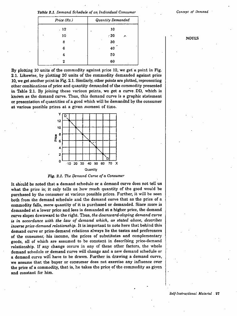
Concept of DemandTable 2.1. Demand Schedule of an Individual Consumer
Price (Rs.) Quantity Demanded
10. 12
10 :-20 Jf'NOTES
8 30
6 40
504
602
By plotting 10 units of the commodity against price 12, we get a point in Fig. 2.1. Likewise, by plotting 20 units of the commodity demanded against price 10, we get another point in Fig. 2.1, Similarly, other points are plotted, representing other combinations of price and quantity demanded of the commodity presented in Table 2.1. By joining these various points, we get a curve. DD, which is known as the demand curve. Thus, this demand curve is a graphic statement or presentation of quantities of a good which will be demanded by the consumer at various possible prices at a given moment of time.
Y D12
10 xa8 \•c0. 6
4
2D
0 10 20 30 40 50 60 70 X Quantity
Fig. 2.1. The Demand Curve of a Consumer
It should be noted that a demand schedule or a demand curve does not tell us what the price is; it only tells us how much quantity of the good would be purchased by the consumer at various possible prices. Further, it will be seen both from the demand schedule and the demand curve that as the price of acommodity falls, more quantity of it is purchased or demanded. Since more is demanded at a lower price and less is demanded at a higher price, the demand
slopes downward to the right. Thus, the downward-sloping demand curvecurveis in accordance with the law of demand which, as stated above, describes inverse price-demand relationship. It is important to note here that behind this demand curve or price-demand relations always lie the tastes and preferences of the consumer, • his income, the prices of substitutes and complementary goods, all of which are assumed to be constant in describing price-demand relationship. If any change occurs in any of these other factors, the whole demand schedule or demand curve will change and a new demand schedule ora demand curve will have to be drawn. Further in drawing a demand curve,
assume that the buyer or consumer does not exercise any influence over the price of a commodity, that is, he takes the price of the commodity as given and constant for him.
we
Self-Instructional Material . 27
Industrial Economy and Principles of Management Reasons for the Law of Demand : Why does Demand Curve
Slope Downward ?We have explained above that when price falls the quantity demanded of a
.commodity rises and vice-versa, other things remaining the same. It is due to this law of demand that demand curve slopes downward to the right. Now, the important question is why the demand cur^'e slopes downward, or in other words, why the law of demand which describe inverse price-demand relationship is valid. We can prove this with marginal utility analysis which we shall explain later in this chapter. It may however be mentioned here that there are two factors due to which quantity demanded increases when price falls :(1) Income Effect. When the price of a commodity falls, the consumer can buy more quantity of the commodity with hisgiocn income. Or, if he chooses to buy the same amount of quantity as before, some money will be left with him because he has to spend less on the commodity due to its lower price. In other words, as a result of the fall in the price of a commodity, consumer’s real income or purchasing power increases. This increase in real income induces the consumer to buy more of that commodity. This is called income effect of the . change in price of the commodity. This is one reason why a con-sumer buys more of a commodity whose price falls.(2) Substitution Effect. The other important reason why the quantity demanded of a commodity rises as its price falls is the substitution effect. When the price of a commodity falls, it becomes relatively cheaper than other commodities. This induces the consumer to substitute the commodity whose price has fallen for other commodities which have now become relatively dearer. As a result of this substitution effect, the quantity demanded of the commodity, whose price has fallen, rises. This substitution effect is more important than the income effect. Marshall explained the downw'ard-sloping demand cur\'e with the aid of thi.s substitution effect alone, since he ignored the income effect of the price change. But in some cases even the income effect of the price change is very significant smd cannot be ignored. Hicks and Allen who put forward an alternative theory of demand called as indifference curve analysis of consumer’s behaviour explain this downward-sloping demand curve with the help of both income and substitution effects.
NOTES
Exceptions to the Law of DemandLaw of demand is generally believed to be valid in most of the situations. However the following exceptions to the law of demand have been pointed out: Goods having Prestige Value. One exception to the law of demand is associated with the name of an economist Thorstein Veblen who put forward the view of conspicuous consumption. According to Veblen, some consumers measure the utility of a commodity entirely by its price, i.e., for them, the greater the price of a commodity, the gi'eater its utility. Diamonds are often given an example of this case. The diamonds are considered as prestige goods in the society and for the upper strata of the society the higher the price of diamonds,
• the higher the prestige value of them and therefore the greater utility or desirability of them. In this case, the consumer will buy less of diamonds at a low price because with the fall in price their prestige value goes down. On the other hand, when the price of diamonds goes up, their prestige value will go up and therefore their utility and desirability. As a result, at a higher price the quantity demanded of diamonds by a consumer will increase.
28 Self-Instructional Material
Concept of DemandGiffen Goods. Another exception to the law of demand was pointed out by Sir Robert Giffin who observed that when the price of bread increased, the low- paid British workers in the early 19th century purchased more bread and not less of it, and this was contrary to the law of demand described above. The reason given for this is that Gitfen goods are inferior goods in .whose case the negative income effect is very large which more than offset the substitution effect. So in their case quantity demanded varies directly with price. After the name of Robert Giffin such goods in whose case there is a direct price-demand relationship are called Giffin goods. It is important to note that when with the rise in price of a commodity, its quantity demanded increases and with the fall in the price of a commodity, its quantity demanded decreases, as in case of Giffen goods, the demand curve will slope upward to the right and not downward. Some other Exceptions. There are some other exceptions to the law of demand which are only apparent and not genuine. In other words, these exceptions to the law of demand are false. One of the false exceptions relates to the changes in the expectations of the people regarding prices of the commodities in the future. Suppose, the rainfall in India in any year does not occur in adequate quantity and there is widespread drought, the expectations of the people will be that the prices would rise in the future. Therefore, even if the prices of foodgrains are higher at the present, they would demand greater quantities since they will be expecting that the prices in the future would be still higher. This is contrary to the law of demand, but in this case to apply the law of demand is not valid. 11116 is because in this case the increase in the quantity demanded is not due to the rise in price but due to the rightward shift in the demand curve as a result of changes in the price expectations of the people. Further, time-series statistical data regarding the quantities purchased of various goods reveal that larger amounts of them have been purchased at higher prices and smaller quantities have been purchased at lower prices over the course of the business cycle. This is also apparently the violation of the law of demand but properly interpreted it does not contradict the law of demand because this only shows that demands for many commodities increase in times of prosperity of the business cycles due to the increase in the incomes of the people, and the demands for the commodities decrease in times of depression of the business cycles due to the fall in the incomes of the people.Another false exception to the law of demand is found when a commodity is sold under two brand names whose prices greatly differ. It is often foimd that some people demand more of a high-priced brand than of the low-priced, although they are almost identical. This author has seen that some of his friends buy more of ‘Supreme Lux’ having a much higher price than ‘Lux’ having a low price even though the two are of almost the same quality. However, this is not a real exception to the law of demand. This is because those who buy more of high-priced brand think that the high-priced brand is different from and superior to the low-priced brand. Therefore, for analysing the nature of demand for these brands, they should be regarded as two different commodities.
NOTES
MARKET DEMAND FUNCTIONFor the business decision making market demand function is of great relevance. As seen above, apart from the determinants of individual’s demand such as price of a product, his income, prices of related commodities, individuals preferences, advertising expenditure, market demand for a product depends on an additional
Self-Instructional Material 2fl
iJndustrioJ Economy anfi Principles of Management
factor, namely the number of consumers which in turn depends on the population of a region or city or country (for which demand is being considered) who consume the product- Mathematically, market demand function for a product can be expressed in the general form as under :
% = AP|, I. P„ T, A, N)where the additional factor is N which stands for the number of consumers or population.For the purpose of estimation of demand for a product we need a specific form of the above market demand function. Generally, it is the linear form which is chosen for estimating market demand function. So in the linear form, the market demand function is given below :
Qo = C + fej P,. > 6,1 + 63F, 6,1 . 6,1' ^ 6,NC is a constant term which shows the intercept of the market demand curve on the X-axis. 6,, 6,, 6g etc. are coefficients (these are generally c^led parameters) which show the quantitative-relationship of various independent variables with the market demand. In other words, these coefficients, 6^, 6,, 63 show how much market demand changes as a result of a unit change in various variables such as price, income, advertising expenditure, population (t.e., the number of consumers).As pointed out in case of individual demand, in economics it is considered important and useful to focus on the relationship between quantity demanded of a product and its price, holding other factors constant. Therefore, if income (I), prices of other related commodities (P^), tastes or preferences of the people (T), advertising expenditure are held constant, the market demand function can be written as
NOTES
%=C*b,P,where C is the constant term in the function or intercept of the market demand curve on the X-axis, b■^ is the coefficient which indicates how much quantity demanded of product X in the market will change as a result of a unit change in its own price, other factors held constant.
Market Demand CurveWe have drawn above an individual’s demand curve of a commodity. We can obtain the market demand curve by making horizontal addition of the demand curves of all individuals buying the commodity. In order to do so we add or sum up the various quantities demanded by the number of consumers in the market. In this way we can obtain the market demand curve for a commodity which like the individual consumer’s demand curve will slope downward to the right. How this summation is done is illustrated in Fig. 2.2. Suppose there are two individual buyers of a good in the market. Fig, 2.2 (ol and (6) show the demand curves of the two independent individual buyers. Now, the market demand curve can be obtained by adding together the amounts of the good which individuals wish to buy at each price. Thus, at price Pj, the individual A wishes to buy 2 units of the good; individual B wishes to by 3 units of the good. The total quantity of the good that the two individuals plan to buy at price Pj is therefore 2 + 3 = 5, which is equal to OQ, in Fig. 2.2 (c).Now. as shall be seen from the figure that at price OP,, individual A demands 4 units and individual B demands 6 units of the commodity. So the market demand at price OP, of the commodity is 4 + 6 = 10 units or OQ,. Similarly.
30 Self-Instructional Material
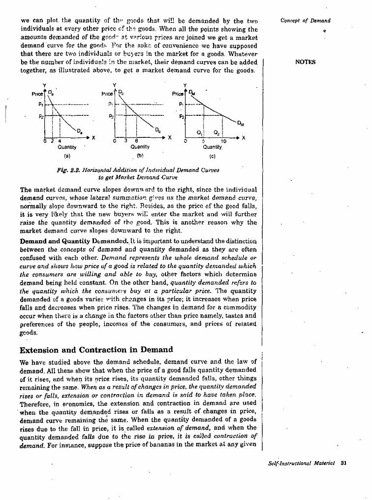
we can plot the quantity of th'’ goods that will be demanded by the two individuals at every other price cf the goods. When all the points showing the amounts demanded of the good'- at various prices are joined we get a market demand curve for the goods For the soke of convenience wc have supposed that there are two individuals or hu>8r3 in the market for a goods. Whatever be the number of individuals in the market, their demand curves can be added together, as illustrated above, to get a market demand curve for the goods.
Concept of Demand
NOTES
‘PcPrice' Pa Price' ‘ RuPrice\P,.\
P-. Pi
02 P2! :iD. IQ,
XX X0 3 6Quantity
0 2 4 5 10Quantity Quantity,
(b)(a) (0
Fig. 2.2. Horizontal Addition of Individual Demand Curves to get Market Demand -Curve
The market demand curve slopes downward to the right, since the individual demand curvos, whose lateral summation gives us the market demand curve, normally slope downward to the right. Besides, as the price of the good falls, it is very likely that the new buyers will enter the market and will further raise the quantity demanded of the good. This is another reason why the market demand curve slopes downward to the right.Demand and Quantity DemandedL.Ib is important to understand the distinction between the concepts of demand and quantity demanded as they are often confused with each other. Demand represents the whole demand schedule or curve and shows how price of a good is related to the quantity demanded which the consumers are willing and able to buy, other factors which determine demand being held constant. On the other hand, quantity demanded refers to the quantity which the consumers buy at a particular price. ITie quantity demanded of a goods variet v'ith changes in its price; it increases when price falls and decreases when price rises. The changes in demand for a commodity occur when there is a change in the factors other than price namely, tastes and preferences of the people, incomes of the consumers, and prices of related goods.
Extension and Contraction in DemandWe have studied above the demand schedule, demand curve and the law of demand. All these show that when the price of a good falls quantity demanded of it rises, and when its price rises, its quantity demanded falls, other things remaining the same. When as a result of changes in price, the quantity demanded rises or falls, extension or contraction in demand is said to have taken place. Therefore, in economics, the extension and contraction in demand are used
■ when the quantity dem_anded rises or falls as a result of changes in price, demand curve remaining the same. When the quantity demanded of a goods rises due to the fall in price, it is called extension of demand, and when the quantity demanded falls due to the rise in price, it is called contraction of demand. For instance, suppose the price of bananas in the market at any given
Self-Instructional Material 81
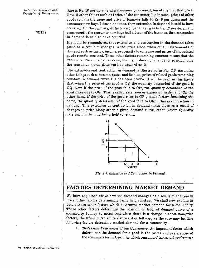
time is Rs. 10 per dozen and a consumer buys one dozen of them at that price. Now, if other things such as tastes of the consumer, his income, prices of other goods remain the same and price of bananas falls to Rs.- 8 per dozen and the consumer now buys 2 dozen bananas, then extension in demand is said to have occurred. On the contrary, if the price of bananas rises to Rs. 12 per dozen and consequently the consumer now buys half a dozen of the bananas, then contraction in demand is said to have occurred.It should be remembered that extension and contraction in the demand takes place as a result of changes in the price alone when other determinants of demand such as tastes, income, propensity to consume and prices of the related goods remain constant. These other factors remaining constant means that the demand curve remains the same, that is, it does not change its position; only the consumer moves downward or upward on it.The extension and contraction in demand is illustrated in Fig. 2.3. Assuming other things such as income, tastes and fashion, prices of related goods remaining constant, a demand curve DD has been drawn. It will'be seen in this figure that when the price of the good is OP, the quantity demanded of the good is OQ. Now, if the price of the good falls to OP', the quantity demanded of the good increases to OQ'. This is called extension or expansion in demand. On the other hand, if the price of the good rises to OP", other factors remaining the same, the quantity demanded of the good falls to OQ". This is contraction in demand. This extension or contraction in demand takes place as a result of ■ changes in price along other a given demand curve, other factors Quantity determining demand being held constant.
Inciusirial Svonomy and Principles of Management
NOTES
Y4D
p..\
I - \Q.
P'
D
O Q" Q Q' Quantity
X
Fig. 2.3. Extension and Contraction in Demand
FACTORS DETERMINING MARKET DEMANDWe have explained above how the demand changes as a result of changes in price, other factors determining being held constant. We shall now explain in detail these other factors which determine market demand for a commodity. These other'factors determine the position or level, of demand curve of a commodity. It may be noted that when there is a change in these non-price factors, the whole curve shifts rightward or leftward as the case may be. The following factors determine market demand for a commodity :
1. Tastes and Preferences of the Consumers. An important factor which determines the demand for a good is the tastes and preferences of tire consumers for it. A good for which consumers’ tastes and preferences
3? Self-Instructional Material
Concept of Demandare greater, its demand would be large and its demand curve will therefore lie at a higher level. People's tastes and preferences for various goods often change and as a result there is change in demand for them. The changes in demand for various goods occur duo to the changes in fashion and also due to the presaure of advertisements by the manufacturers and sellers of different products. On the contrary, when certain goods go out of fa.shion or people’s tastes aj^d preferences no longer remain favourable to them, the demand for them decreases.
2. Income of the People. The demand for goods also depends upon the incomes of the people. The greater the incomes of the people, the greater will be their demand for goods. In drawing the demand schedule or the demand curve for a good we take income of the people as given and constant- When as a result of tho rise in the income of the people, the demand increases, the whole of the demand curve shifts upward and vice-versa. Tlte greater income means thegreate?' purchasing power. Therefore, when the incomes of the people increase, they can afford to buy more. It is because of this reason that the increase in income has a positive effect on the demand for a good. When the incomes of the people fall they would demand les.s of a good and as a result the demand curve will shift downward. For instance, during the planning period in India the incomes of the people have greatly increased owing to the large investment expenditure on the development schemes by the Government and the private sector. As a result of this increase in incomes, the demand for good grains has greatly increased which has resulted in the food problem. Likewise, when because of drought in a year the agriculture production greatly falls the incomes of the farmers decline. As a result of the decline in incomes of the farmers, they will demand less of the cotton cloth and other manufactured products.
3. Changes in Prices of the Related Goods. The demand for a good is also affected by the prices of other goods, especially those which are related to it as substitutes or complements. When we draw the demand schedule or the demand curve for a good we take the prices of the related goods as remaining constant. Therefore, when the prices of the related goods, substitutes or complements, change, the whole demand curve would change its position; it will shift upward or downward as the case may be. When the price of a substitute for a good falls, the demand for that good will decline and when the price of the substitute rises, the demand for that good will increase. For example, when the price of the tea as well as the incomes of the people remain the same but the price of the coffee falls, the consumers would demand less of tea than before. Tea and coffee are very close substitutes. Therefore, when coffee becomes cheaper, the consumers substitute coffee for tea and as a result the demand for tea declines The goods which are complementary with each other, the change in the price of any of them would favourably affect the demand for the other. For instance, if the price of milk falls, the demand for sugar would also be affected. When people would take more milk, the demand for sugar will also increase. Likewise, when the price of cars falls, the quantity demanded of them would increase which in turn will increase the demand for petrol.
NOTES
Self-Instructional Malrriol 33
h rluslrial Economy and l‘r:iir!l>lcs of Management 4. Advertisement Expenditure: Advertisement expenditure made by a
firm to promote tiie sales of its product is an important factor determining demand for a product, especially of the product of the firm which gives advertisements. The purpose of advertisement is to influence the consumers in favour of a product- Advertisements arc given in various media such as newspapers, radio, television. Advertisements for goods are repeated several times so that consumers are convinced about their superior quality. When advertisements prove successful they cause an increase in the demand for the product.
5- The Number of Consumers in the Market. Wc have already explained that the market demand for a good is obtained by adding up the individual demands of the present as well as prospective consumers
• of a good at various possible prices. The greater the number of consumers of a good, the greater the market demand for it. Now', the question arises on what factors the number of consumers for a good depends. If the consumers substitute one good for another, then the number of consumers for the good which has been substituted by the • other will decline and for the good which has been used in place of the other, the number of consumers will increase. Besides, when the seller of a good .succeeds in finding out new markets for his good and as a result the market for his good expands, the number of consumers for that good will increase. Another important cause for the increase in the number of consumers is the growth in population. For instance, in India the demand for many essential goods, especially foodgrains. has increased because of the increase in the population of the country and the resultant increase in the number of consumers for them.
6. Consumers’ Expectations with regard lo'Future Prices. Another factor which influences the demand for goods is consumers' expectations w'ith regard to future prices of the goods. If due to some I'eason, consumers expect that in the near future prices of the goods-would rise, then in the present they would demand greater quantities of the goods so that in the future they should not have to pay higher prices. Similarly, when the consumers hope that in the future the prices of good will fall, then in the present they will postpone a part of the consumption of goods with the result that their present demand for goods will decrease.
NOIES
Shifts in Demand : Increases and Decreases in DemandWhen demand changes due to the factors other than price, there is a shift in the whole demand curve. As .mentioned above, apart form price, demand for a commodity is determined by incomes of the consumers, his tastes and preferences, prices of related goods. Thus, when there is any change in these factors, it will cause a shift in demand curve. For example, if incomes of the consumers increase, say due to the hike in their wages and salaries or due to the grant of dearness allowance, they will demand more of a good, say doth, at each price. This will cause a shift in the rismaiid curve to the right as is shewn in Pig. 2.4. To being with DD is the demand curve. With the increase in income, the demand curve shifts to the right to D'D' which implies that f-r. each price such as Pj, Pj Pj the consumers demand more of the commodity than before. Similarly, if preferences of the people for a cemmodity, say colour T'V, become greater, their demand for colour TV will increase, that is, the demand curve
34 Srlf'l’mlruclional Material
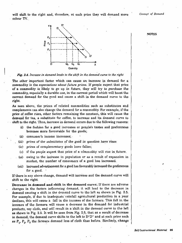
Coiicepi of Demandwill shift to the right and, therefore, at each price they will demand more colour TV.,
NOTESP3
8£
Pi
Cb Qz Qio XQuantity
Fig. 2.4. Increase in demand leads to the shift in the demand curve to the right
The other important factor which can cause an increase in demand for a commodity is the expectations- about future prices. If people expect that price of a commodity is likely to go up in future, they will try to purchase the commodity, especially a durable one, in the current period which will boost the current demand for the good and cause a shift in tiie demand curve to the right.As seen above, the prices of related commodities such as substitutes and complements can also change the demand for a commodity. For example, if the price of coffee rises, other factors remaining the constant, this will cause the demand for tea, a substitute for coffee, to increase and its demand curve to
. shift to the right. Thus, increase in demand occurs due to the following reasons:(i) the fashion for a good increases or people’s tastes and preferences
becomes more favourable for the goods;(u) consumer’s income increases; •
(Ui) prices of the substitutes of the good in question have risen (iy) prices of complementary goods have fallen;(y) if the people expect that price of a commodity will rise in future,
(yi) owing to the increase in population or as a result of expansion in market, the number of consumers of a good has increased.
(vii) increased advertisement for a good has favourably increased the preferences for a good.
If there is any above change, demand will increase and the demand cun/e will shift to the right.Decrease in demand and shift in the demand curve. If there are adverse changes in the factors influencing demand, it will lead to the decrease in demand causing a shift in the demand curve to the left as shown in Fig. 2.5. For example, if due to inadequate'rainfall agricultural production in a year declines, this will cause a fall in the incomes of the farmers. This fall ir. the incomes of the farmers \vill cause a decrease in the demand for industrial products, say cloth, and will result in a shift in the demand curve to the left as shown in Pig. 2.5. It will be seen from Fig. 2.5, that as a result of decrease in demand, the demand curve shifts to the left to D''D" and at each prict? such as P,. P„, P» the farmers demand less, of cloth than before. Similarly, change '
A* o
Self-Instructional Materiol 35
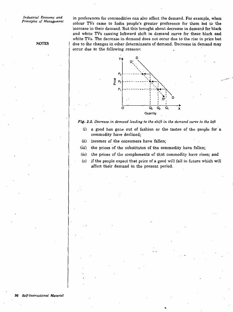
Industrial Economy and principles of Management
in preferences for commodities can also affect the demand. For example, when colour TVs came to India people's greater preference for them led to the increase in their demand. But this brought about decrease in demand for black and white TVs causing leftward shift in demand curve for these black and white TVs. The decrease in demand does not occur due to the rise in price but due to the changes in other determinants of demand. Decrease in demand may occur due to the following reasons;
NOTES
DYD”
NN
NS
Pz8£ s I
'n IPi
II N II '♦ ' DI D"IfI1I
O 03 Q? Q, XQuarVSy
Fig. 2.5. Decrease, in demand leading to the shift in the demand curve to the left
(i) a good has gone out of fashion or the tastes of the people for a commodity have declined;
Qi) incomes of the consumers have fallen;(Hi) the prices of the substitutes of the commodity have fallen;(iv). the prices of the complements of that commodity have risen; and(o) if the people expect that price of a good will fall in future which will
affect their demand in the present period.
I
t
36 Self-Instructional Material
\
Concept of Demand
STUDENH^CIiVITy
1. What do you mean by demand ? Explain the law of demand with an illustration.
2. State the law of demand. Give circumstance under which it is not operative.
Seif-Instruciional Material 37
Industrial Economy and Principles of Management SUMMARY
• According to the law of demand, other things being equal, if the price nf a commodity falls, the quantity demanded, of it will rise, and if the price of the commodity rises, its quantity demanded will decline.
• When the quan!;ilv demanded nf a goods rises due to the fall in price, it is called extension of demand, and when the quantity demanded falls due to the rise in price, it is called contraction of demand.
• When the price, of a substitute for a good falls, the demand for that good will decline and when the price of the substitute rises, the demand for that good will increase.
NOTES
REVIEW EXERCISES1. What factors determine the demand of a commodity ? Explain.2. Explain demand schedule and demand curve of an individual 'with the
help of an illustration.3. Explain the reasons of demand curve sloping downward.4. Explain law of demand and discuss the rationale for this law.5. What are the exceptions to the law of demand ? Discuss.6. Describe the impact of rise in income on normal goods and inferio''
goods.7. What do.you mean by expansion and contraction in demand? Explain
with the help of a diagram.8- Briefly discuss the impact of increase and decrease in demand on the
demand curve.•9. Explain income effect and substitution effect on the demand of a
commodity.
38 Self-Instructional Material
Concept of Supply
UNIT 3 CONCEPT OF SUPPLY
★ STRUCTURE ★ NOTES
□ The Meaning of Supply
□ Changes in Supply ; Increase and Decrease in Supply□ Elasticity of Supply
Price of a commodity is determined bv the demand for and supply of a commodity. In some previous chapters we have studied the factors which determine the demand for a commodity. We have also studied the law of demand according to which the demand for' a commodity is inversely related to its price. Supply of a commodity depends upon how the physical returns and costs change as ■more output of a commodity is produced. After having explained the behaviour of costs and physical returns in the previous chapters, we are now in a position to explain the law of supply and the concept of elasticity of supply.
THE MEANING OF SUPPLY, demand is defined as a schedule of the quantities of a good that will be
purchased at various prices, similarly the supply refers to the schedule of the quantities of a good that will be offered for sale at various prices. To be more correct, supply of a commodity is the schedule of the quantities of a commodity that would he offered for sale at all possible prices at any moment of time or during any one period of time, for example, a day, a week and so on, the conditions of supply remaining the same.Supply should be cai-pfully distinguished from stock, Sfoc^ is the total volume of a commodity winch can be brought into the market for sale at a short notice and supply means the quantity which is actually brought in the market. For perishable commodities like fish and fruits, supply and stock are the same because whatever is in the stock must be disposed of. The commodities, which are non-perishable, can be held back if prices are not favourable. In case of a non-perishable or durable commodity if the price is high, larger quantites of it are offered , by the sellers from their stock. And if its price is low, only small quantities are brought out for sale. In short, stock is potential supply.
Supply Schedule, Supply Curve and Law of SupplySupply ot a commodity .is functionally related to its price. The law of supply relates to this functional relationship between price of a commodity and its supply. In contrast to the change in quantity demanded in response to the changes in price, the quantity supplied generally varies directly with price. That is, the higher the price, the larger is the quantity supplied. The supply schedule nr supply curve of a commodity means how price of a commodity is related to the quantity which the sellers (or producers) are willing and able to
Self-Instructional Material 39
Industrial Economy and Principles of Management
make available in the market. The supply schedule giving various prices of wheat and quantities of wheat supplied at those prices is shown in Table 3.1. It will be seen from this table that at a price of Rs. 275 per quintal sellers are willing and able to supply 200 quintals of wheat. When the price of wheat rises to Rs. 325 per quintal, the greater quantity (300 quintals) of it is supplied in the market. If the price of wheat further goes upto Rs. 375, the still greater quantity 400 quintals are offered for sale in the market by the suppliers.
Table 3.1. Supply Schedule
NOTES
Price (Rs.) Quantity Supplied
225 100275 200325 300375 400425 500
It is important to note that like the concept of demand, the concept of supply does not refer to a fixed quantity of a good which the sellers are willing and able to make available in the market. Instead, the supply of a commodity implies how the quantity supplied of the commodity varies with the change in price under the given conditions of cost and technology. Thus, supply refers to the whole schedule or curve depicting the relationship between price and quantity which the sellers produce and offer for sale in the market.Law of supply. The supply schedule and supply curve reflect the law . supply. According to the law of supply, when the price of a commodity rises the quantity supplied of it in the market increases, and when the price of a commodity falls, its quantity demanded decreases, other factors determining supply remaining the same. Thus, according to the law of supply, the quantity supplied of a commodity is directly or, positively related to price. It is due to this direct relationship between price of a commodity and its quantity supplied that the supply curve of a commodity slopes upward to right as seen from supply curve SS in Fig. 3.1. When price of wheat rises from Rs. 225 per quintal to Rs. 426 the quantity supplied of wheat in the market increases from 100 quintals to 600 quintals per period.
S425
37S
325
275
225S
o 100 200 300 400 500Quanbty
Fig. 3.1. Supply Curve Showing Direct Relationship Between Price and Quantity
40 Self-Instructional Material
Concept of SupplyWhy Does Supply Curve Generally Slope Upward to the Right ?In a .later chapter we will explain in detail why supply is directly related to price or supply curve generally slopes upward to the right. The law of supply or upward-sloping supply curve implies that only at a higher price of a good, more quantity of it will be produced and made available in the market during a given period. Why at a higher price, more quantity of a good is supplied? The reason is that at a higher price of the commodity, other things remaining the same, the greater the potential profits which producers can generally expect from producing and supplying it in the market. The law of supply and positively sloping supply curve is based upon two important assumptions. First, producers or sellers aim to maximise profits from production and sale of a commodity. Secondly, as output of a commodity is expanded, the additional cost of producing an extra unit goes up due to diminishing returns to the variable factors.lb understand why more is supplied at a higher price, during a given period, let us illustrate it with an example. Suppose the demand for ready-made shirts in a given period increases, the firms producing them cannot easily increase the factory space and machinery used in the production of ready-made shir^ in the short run. The firms will expand their output by employing more of the variable factors which can be easily increased in the short-run such as labour and cloth (which is the raw material for producing shirts), keeping other factors fixed. But the as factory-space, machinery will cause the total output of shirts to increase at a diminishing rate. In economic terms, it is said that the diminishing marginal returns accrue to the extra units of labour and other variable factors employed to expand output to meet the increased demand for the shirts. In order to maximise profits, the producer will equate price of a product with the additional or marginal cost of producing a unit of output. Since the marginal cost of a unit of output increases as output is expanded due, to the occurrence of diminishing marginal returns to the variable factors, the producer will be willing to produce and make available in the market more quantity of a commodity only at a higher price.It may however be noted that if diminishing marginal returns to factors do not occur and therefore marginal cost does not rise with the expansion in output as may be the case in the long run when all factors including fixed factors such as factory-space and machinery can be easily increased, the supply curve of output will be a horizontal straight line and the law of supply will not hold. Thus, it is the rising marginal cost of additional units of output coupled with the objective of maximising profits on the part of producers that explain the upward-sloping supply curve of output which reflects the law of supply.It is important to note that each point on the supply curve indicates the price at which a given quantity of output the producers will be willing to supply, that is, make it available in the market. The price at which a given quantity of the commodity is supplied by the sellers is called supply price. The upward-sloping supply curve indicates that the supply price increases if more quantity of the good is to be supplied in the market. Thus, the greater the quantity which the consumers would like to buy, the higher the price necessary to induce the producers to produce a commodity and make it available in the market.Supply and Quantity Supplied. As in case of demand and quantity demanded, the supply should not be confused with the quantity supplied- Whereas the supply describes the whole schedule or curve depicting the relationship between price and quantity supplied in a period, the quantity supplied refers to the
NOTES
Self-Instructional Material 41
Industrial Economy and Principles of Management quantity which the producers would make it available at a particular price of
the commodity. As seen above, the quantity supplied varies with a change in price of a commodity. Thus, change in quantity supplied of a commodity' occurs
• in response to a change in its price; at a higher price, more quantity of it is supplied and vice-versa. For example, in our illustration given above, when price of wheat rises from Rs. 225 to Rs. 425 per quintal, the quantity supplied of wheat increases from 100 quintals to 500 quintals, the supply schedule or supply curve being given.The terms extension and contraction in supply are used for changes in quantity supplied as a result of changes in price of a commodity. When the me in price of a ccmmodity brings about increase in quantity supplied of the commodity, other factors determining supply remaining constant. Ihis is called I'yte.rsion in supply. On the other hand, when price of a commodity falls and as a result, the quantity supplied of it decreases, contraction in supply is said to have occurred, other factors being held constant.Thus extension in supply should be carefully distinguished from increase in supply. While extension in supply of a commodity occurs as a result of rise in price of the commodity, increase’ in supply means that due to reduction in prices of resources improvement in technology, whole supply curve shifts to the right showing more is supplied than before at each price of the commodity.Similarly, there is contraction in supply of a commodity when its price falls, that is, when a smaller quantity of it is supplied at a lower price whereas decrease in .supply implies that because of rise in prices of resources, imposition of excise duty, etc., the entire supply curve shifts to the left so that less quantity of the commodity is supplied at every price.
NOTES
CHANGES IN SUPPLY : INCREASE AND DECREASE IN SUPPLYAs stated above, the supply of a commodity in economics means the entire schedule or curve depicting the relationship between price and quantity supply of the commodity, the other factors including supply remaining constant. These other factors are the state of technology, prices of inputs (resources), prices of other related commodities, etc. which arc assumed constant when the relationship between price and quantity supplied of a commodity is examined.It is the changes in these factors that cause a shift in the supply schedule or curve. Thus a change in supply refers to the shift in the supply curve due to the changes in factors other than price. For example, when prices of inputs such as labour and raw materials used for the production of a commodity decline, this will result in lowering the cost of production which will induce the producers to produce and make available greater quantity of the commodity in the market at each price. This means increase in supply has taken place. This increase in supply of a commodity due to the reduction in prices of input-s will cause the entire supply curve to shift to the right as shown iii Fig. 3.2, w'here the supply curve shifts from SS to S'S'. As shown by arrow marks, at prices Pj, Pj and P3, quantity supplied increases when supply increases causing a rightward shift in the supply curve. Similarly, progress in technology used for production of a commodity will also cause a shift in the supply curve to the right.
42 Self-Instructional Material

Concept of SupplyY‘YS' SS'
/
I £ NOTESP2A Pi
PiPt
sS'I X♦ X0 o Qi Qs CbQ, Qz Qs QuanMty
Fig. S,2. Increase in Supply Causing a Rightward Shift in the Supply Curve
On the other hand, decrease in supply means the reduction in quantity supplied at each price of the commodity as shown in Fig. 3.3 where as a result of decrease in supply, the supply curve shifts to the left from SS to S"S". As shown by the arrow marks, at each price such as Pj, Pj, Pg the quantity supplied on the supply curve S"S'' has declined as compared to the supply curve SS. The decrease in supply occurs when the prices of factors (inputs) used for the production of a commodity go up so that each quantity of the commodity is produced at a hi^er cost per unit which causes a reduction in quantity supplied at each price. Similarly, the imposition of an excise duty or sales tax on a commodity means that each quantity will now be supplied at a higher price than before so as to cover the excise duty or sales tax per unit. This implies that quantity supplied of the commodity at each price will decrease as shown by the shift of the supply curve to the left.Another important factor causing a decrease in supply of a commodity is the ris^ in prices of other commodities using the same factors. For example, if the
• price of wheat rises sharply, it will become more profitable for the farmers to grow it. This will induce the farmers to reduce the cultivated area under other crops, say sugar cane and devote it to the production of wheat. This will lead to decrease in supply of sugar cane whose supply curve will shift to the left. Further, agricultural production in India greatly depends on the rainfall due to monsoon. If monsoon come in time and rainfall is adequate, there are bumper crops, the supply of agricultural products increases. However, in a year when monsoon are untimely or highly inadequate, there is a sharp drop in agricultural production causing a decrease in the supply of agricultural output and thereby shift the supply curve of agricultural output to the left. We thus see that there are several factors other than price which determine the supply of commodity and any change in them causes a shift.in the entire supply curve.
QuanUtyFig. 3.S. Decrease in Supply Causing a
Leftward Shift in the Supply Curve
Factors Determining SupplyIt is clear from the supply schedule (Table 3.1) and the supply curve (Fig. 3.2) given above that the quantity supplied varies directly with the price of a product. A supply schedule and supply curve show that the supply of a product is function of its price. However, the supply depends not only on the price of a product but on several other fsictors too. We have seen above that the effect of changes in price of a product on the quantity supplied of it is explained by a movement along a given supply schedule or curve, the effect of other factors is represented by the shifts in the entire supply schedule or supply curve.
Self-Instructional Material 43
Industrial Economy and Principles of Management While making a supply schedule or a supply curve we assume that these other
factors remain the same. Thus when these other factors change, they shift in the entire supply curve. The factors other than price which determine price are the following :
(а) Production Technology. A change in technology affects the supply function by altering the cost of production. If there occurs an improvement in production technology used by the firms, the cost of production declines and consequently the firms would supply more than before at the given price. That is, the supply would increase implying that the supply curve would shift to the right.
(б) Prices of Factors. Changes in prices of factors or resources also cause a change in the cost of production and consequently bring about a change in supply. For example, if either wages of labour increase or prices of raw materials and fuel go up, the unit cost of production will rise. With a higher unit cost of production, less would be supplied than before at various prices. This implies that supply curve would shift to the left.
(c) Prices of Other Products. When we draw a supply curve we assume that the prices of other products remain unchanged. Now, any change in the prices of other products would influence the supply of a product by causing substitution of one product for another. For example, if the market price of wheat rises, it will lead to the reduction of the production and supply of gram by the farmers as they would withdraw some land and other resources from the production of gram and devote them to the production of wheat. This will cause a leftward shift in the supply curve of gram.
(d) Objective of the Firm. The objective of a firm also determines the supply of a product produced by it. If the firms aim to maximize sales or revenue rather than profits, the production of the product produced by it and hence the supply of it in the market would be larger.
(c) Number of Producers (or Firms). If number of firms producing a product increases, the market supply of the product will increase causing a rightward shift in the supply curve. When, in the short- run, firms in an industry are making large profits, new firms enter that industry in the long-run and expand the total production and supply of the product of that industry. On the other hand, due to losses when some firms leave the industry, the supply of its product will decrease and supply curve will shift to the left.
(/) Future Price Expectations. The supply of a commodity in the market at any time is also determined by sellers’ expectations of future prices. If, as happens during inflationary periods, sellers expect the prices to rise in future, they would reduce supply of products in the market and would instead hoard them. The hoarding of huge quantities of goods by traders is an important factor in reducing supplies in the market and thus causing further rise in their prices.
ig) Taxes and Subsidies. Taxes and subsidies also influence the supply of a product. If an excise duty or sales tax is levied on a product, the firms will supply the same amount of it at a higher price or less quantity of it at the same price. This implies that imposition of a sales tax or excise duty causes a leftward shift in the supply curve.
cause a
NOTES
44 Self-Instructional Material
Concept of SupplyThe opposite happens case of the supply of a commodity on which the government provides subsides.
It follows from above that technology, prices of factors and other products, expectations regarding future prices and objective of the firms are the important determinants of supply which cause rightward or leftward shift in the whole supply curve. NOTES
ELASTICITY OF SUPPLY■ When a small fall in the price of a commodity leads to a large contraction in
supply, the supply is comparatively elastic. But when a big fall in price leads to a very small contraction in supply, the supply is said to be comparatively inelastic. Conversely, a small rise in price leading to a big extension in supply shows elastic supply, and a big rise in price leading to a small extension in supply indicates inelastic supply.Consider Pigs. 3.4 and 3-5 where two supply curves SS have been drawn. At price OP,, the quantity supplied in Fig. 3.4 is OQ,, and the quantity supplied in Fig. 3.5 is ON,. With rise in price of the product, quantity supplied increases from OQ to OQg in Fig. 3,4 and from ON, to ONg in Fig. 3.5. Whereas the relative change in price' is the same in both the figures, the increase in quantity supplied Q,Q2 in Fig. 3.4 is much larger as compared to the increase in quantity supplied N.Nj in Fig. 3.5. Therefore, supply in Fig. 3.4 is said to be elastic, whereas that in Fig. 3.5 is ineiastic. The elasticities of supply of various products differ very much from each other. What are the factors which determine elasticity of supply of products will be explained in some detail later.
Y AY S
P2P2
PiPi
88££
XoXoNi N2
Quantity
Fig. 3.S, Inelastic Supply
02QiQuantity
Fig. 3.4. Elastic Supply
The concept of elasticity of supply, like the elasticity of demand, is a reltative > of the responsiveness of quantity supplied of a commodity to a changemeasure
in its price. The greater the responsiveness of quantity supplied of a commodity to the changes in its price, the greater its elasticity of supply. In precise terms, the elasticity of supply can be defined as a percentage change in the quantity supplied of a product divided by the percentage change in price that caused the change in quantity supplied.
Percentage chai^ in quantity suppliedPercentage change in priceElasticity of supply =
aPAQ xlOO- xlOOe* = PQ
Self-Insiructional Material 45
Indu!<trial Economy and Principles of Management AQ P
S —X-------
Q APAQ P
s= ——AP Q
If the price of a refrigerator rises from ns. 2,000 per unit to Rs. 2,100 per unit and in response to this rise in price, quantity supplied of it increases from 2,500 units to 3,000 units, the elasticity of supply will be
500 2000 100 2500
If the ev.pply cu’^ve of a commodity is upwgrd as is generally the case(See Figs, 3.4 and 3,5), the '■oefflcient of elest’C’ty '■unr'iy '.v’V t-sve a positive sign. When the supply curve is upward sloping, the °!asticity supply will be anything between zero and infinity. When the quantity supplied of a commodity does not change at all in response to the changes in its price, the elasticity of supply is zero. In the case of zero elasticity of supply, the supply curve will be a vertical straight line parallel to the Y-axis and is said to be perfectly inelastic (See Fig. 3.6). On the other hand, if at a price any quantity of a good can be supplied, its elasticity will be equal to infinity and its supply curve will be a , horizontal straight line parallel to the quantity axis and is said to be perfectly elastic (See Fig. 3.7).
NOTES
20 - = 5 X — = 4= 25.
YsY
ss'a. S•c S0.
♦ X o X •o s QuantityQuantity
Fig. 3.6. Perfectly Inelastic Supply Fig. 3.7. Perfectly Elastic Supply
Measuring Elasticity of Supply at a Point on tb#» Supply CurveNow, an important question is how elasticity of supply can be measured at a point on a given supply curve. Consider a linear supply curve SS drawn in Pig. 3.8 where we are required to measure elasticity of supply at point R on it corresponding to output OQ and price OP. In order to measure supply elasticity at point R we extend the supply curve so that it meets the X-axis at point T. Then measure of elasticity of supply at poiiu h. can oe obtained by dividing the distance TQ by the distance OQ, Thus
TQSupply elasticity at point R on supply curve SS (e^) =
Proof. That the elasticity of supply at point K on the supply curve SS in Fig. TQ
3.8 is given by ’ can be easily proved as under ;OQAQ P AP Q=
46 Seif-Jnstructional Material
Y Concept of SupplyS
8•cCL NOTES
ii/p
se
XT O Q Quantity
Fig. 3.8. Measuring Elasticity of Supply
AQThe term — an the elasticity formula is '•he redprocal of the slope, of supply
APcurve SS (note that the slope of the i'''r,ly cnr\'e is equal to
Thus, rewriting the measure of the coefficient of supply elasticity we have
)dQ ■
! P= slope Q
Now consider Pig. 3.S. Th* slope of the ;7Upp3y cun'e SS is equal to RQTQ, price at point R is RQ and quantity supplied is equal to OQ. Substituting these values in the formula for coefficient of supply elasticity we have
1 P slope Q
1 RQ TQ RQ TQ RQ^'tQ RQ’'0Q'"bQ'
=
TQ
Thus elasticity of supply is given by the ratio of distance TQ and OQ.In Fig-3.8, the supply curve when extended meets the X-axis to the left of the
TO—-2- will thereforepoint of origin, TQ is greater than OQ. elasticity coefficientuy
be greater tiian on-:.In Fig- 3.9 supply curve when extended meets the X-axis to the right of the point of origin so that TQ is smaller than OQ. Therefore, in Fig. 3.9 the
TOel«-sticity of supply ^ is less than unity. In Fig. 3.10 supply curve when OQ
extended mcet.s the X-axis exactly at the point of origin so that TQ i.s equal to OQ- Therefore in Fig,-3.10 elasticity of supply will he equal to one.In Fig. 3.8 claHiciv' of supply will be greater than one at every point of she supply curve, hut it will differ from point to point. Similarly in Fig. 3.9 supply elasticity is less than one at every point of the supply curve, but it will differ from point to point. However, in Fig- 3.10 elasticity of supply will be equal to one at every point of the supply curve.
Self-Insitructinnal Material 47
Industrial Economy' and Principles of Management
Y YS S
s u1
ppNOTES
TO X /o QT OQuantityQuantity '
Fig. 3.9. e, < 1 Fig. 3.10. = I
Point Elasticity of Supply on a Non-linear Supply CurveWe have studied above how the elasticity of supply is measured at a point on a straight line supply curve. But now the question is how the'point elasticity of supply can be measured on a non-linear supply curve. Consider Fig. 3.11 where a non-linear supply curve has been drawn and it is required to measure elasticity at point A on it. The general principle involved is the same as derived above. In order to apply the above principle for estimating the elasticity of supply at point A on the supply curve SS, we have to draw a tangent at it. Now, a tangent has been drawn at point A. On being extended, tangent meets the X-axis at point Tj.
Therefore, elasticity of supply at point A on the supply curve is = T,Q:OQ,
: Y
O'
Qusntitj'
Fig. 3.11. Varying Elasticity of Different Points on the Supply Curve
Likewise, we can find out the elasticity of supply at point B on the supply .curve. For this, tangent drawn at point B and has been extendedto meet the X-axis at point T,. Thus, price elasticity at point B on the supply
TiQ,curve SS is equal to . It is also evident from Fig. 3.11 that price elasticity
T,Q.
T, Q2
T2Q ^ is less thanof supply at point A and B is different. Since priceOQ,elasticity of supply at point B is less than that at A.
OQ, ’
48 Self-Instructional Material
Factors Determining Elasticity of SupplyElasticity of supply plays an important role in determining prices of products. To what extent price of a product will rise following the increase in demand for it depends on the elasticity of supply. The greater the elasticity of supply of a product, the less the rise in its price when demand for it increases. We explain below the factors which determine price elasticity of supply of a product. The Changes in Marginal Cost of Production. Elasticity of supply of a commodity depends upon the case with which increases in output can be obtained without bringing about rise in cost of production. If with the increase in production, the marginal cost of production goes up, the elasticity of supply to that extent would be less. In the short-run, with some factors of production being fixed, the increase in the amount of a variable factor eventually causes diminishing marginal returns and as a result with the expansion of output marginal cost of production rises. This causes supply of a commodity in the short run less elastic. However, in the long-run, the firms c&n increase output by varying all factors and also the new firms can enter the industry and thereby add' to the supply of a commodity. Therefore, the long-run supply curve of a commodity is more elastic than that of the short-run.In the increasing cost industry, that is, the industry which experience increases in cost when industry expands through the entry of new firms, the 1 g-run. supply curve, like the short-run one, is upward sloping, but will be more elastic than in a short-run. In the constant cost industry, i.e., the industry wherein there are neither net external economies and nor net external diseconomies, the long-run supply curve, as has been stated above, is perfectly elastic because in this case increases in the industrial output can be obtained at the same cost of production, that is, without raising average and marginal cost curves. In the decreasing cost industry, that is, industry which is subject to increasing returns, long-run supply curve is downward sloping and has therefore a negative elasticity of supply. This is because in the case of decreasing-cost industry expansion in the industry brings down the cost of production and therefore additional output is forthcoming at a lower supply price.Behaviour Pattern of the Producers. Besides the change in cost of production, the elasticity of supply for a product depends on the responsiveness of producers to changes in its price. If the producers do not respond positively to the increase in prices, the quantity supplied of a product would not increase as a result of rise in its price. A profit-maximising producer will increase the quantity supplied of a product following the rise in its price. However, producers do not always exhibit profit maximizing behaviour, as is generally assumed in economic theory and as a result do not raise supply in response to the rise in price. For example, it has been argued by some with some empirical evidence that farmers in developing countries respond negatively to the rise in price of their agricultural products. They point out that at higher agricultural prices, their need for fixed money income is met by selling smaller quantities of foodgrains and therefore at higher prices they produce and sell smaller quantities rather than more.Availability of the Production Facilities for Expanding Output. Theextent to which the producers would raise supply of their products also depends
the availability of productive facilities and inputs required for the production of goods. For example, when there is lack of fertilisers, irrigation facilities, the farmers would not be able to raise the supplies of agricultural products in response to the rise in their prices even if they want to do so. Likewise, in the industrial fie!d-if there is shortage of power, fuel, essential raw materials, the
Concept of Supply
NOTES
on
Self-Instructional Material 49
Industrial Economy and Principles of Management expansion in supply would not be forthcoming in response to the rise in prices
of industrial products.Possibilities of Substitution of One Product for the Others. The change in quantity supplied of a product following the changes in its price depends on the possibilities of substitution of one product for others. For example, if market price of wheat rises, the farmers will try to shift resources such as land, fertilisers away from other products such as pulses to devote them to the production of wheat. The greater the extent of possibilities of shifting of resources from the other products to wheat production, the greater the elasticity of supply of wheat.The Length of Time. The elasticity of supply of a product also depends on the length of time during which producers have to respond to a given change in price of a product. Generally, the longer the time producers get. to make adjustments for changing the level-of output in response to a change in price, the greater the response of output, that is, the greater the elasticity of supply. From the viewpoint of the influence of the length of time on the elasticity of supply we distinguish between three time periods : (1) market period or very short run, (2) short run and (3) long run. In the market period no more production is possible. Therefore, market period supply curve is a vertical straight line (i.e., perfectly inelastic). In the short-run, firms can change output by changing the amounts of only variable factors, short-run supply curve is somewhat elastic. In the long run since firms can adjust all factors of production and also new firms can enter or leave the industry, long-run supply curve is more elastic.
NOTES
50 S«^-ftlstruciionai Moterinl
Concept of Supply
STUDENT ACTIVITY
1. What do you mean by supply ? What -are the reasons for the change in supply ?
2. Explain the concept of supply. Distinguish between supply and stock.
Self-Instructional Material 51
Industrial Economy and Principles of Management SUMMARY
• Stock is the total volume of a commodity which can be brought into the market for sale at a short notice and supply'means the quantity which is ocfuaHy brought in the market.
• The price at which a given quantity of the commodity is supplied by the sellers is called supply price.
• When a small fall in the price of a commodity leads to a large contraction in supply, the supply is comparatively elastic. But when a big fall in price leads to a very small contraction in supply, the supply is said to be comparatively inelastic.
NOTES
REVIEW EXERCISESWhat is meant by supply ? Explain the law of supply with the help of supply schedule and curve.Define the terra elasticity of supply. Explain its measurement with an illustration.What factors determine the supply ? Explain with examples. Describe elasticity of supply. Discuss its main types.Explain the concept of elasticity of supply and describe the factors that affect elasticity of supply.Explain the law of supply with the help of a supply schedule and supply curve.How is elasticity of supply measured ? What are the various determinants of supply elasticity ?State the law of supply and describe the shape of supply curve.Explain the situations when the elasticity of supply is more than one and less than one.Briefly answer the following ;(a) Define the concepts of supply and stock. ib) Explain elasticity of supply.(c) State the law of supply.
id) Enumerate the determinants of elasticity of supply.(e) What is the shape of supply curve ?(/) Explain contraction and expansion of supply.
1.
2.
3.4,5,
6.
7.
8.9.
10.
62 Self-Instructional Material
Theory of Consumer's Bahaviour Utility AnalysisUNIT 4 THEORY OF CONSUMER'S
BEHAVIOUR UTILITY ANALYSISNOTES
★ STRUCTURE ★□ Introduction□ The Meaning of Utility□ Law of Diminishing Marginal Utility
INTRODUCTIONThe price of a product depends upon the demand for and the supply of it. In this part of the book we are concerned with the theory of demand, which explains the demand for a good and the factors determining it. The factors governing the supply of a good will be discussed in the next part of the book. Individual’s demand for a product depends upon the price of the product, income of the individual, the prices of related goods. It can be stated in the following functional form;
D, * APx. I> P,. P* etc.)where stands for the demand for good X, for price of good X, I for i'’dividual’s income, P^, etc., for the prices of related goods. But among these determinants of demand, economists single out price of the good in question as the most important factor governing the demand for it. Indeed, the function of a theory of demand is to establish a relationship between quantity demanded of a good and its price and to provide an explanation for it.From time to time, different theories have been advanced to explain consumer’s demand for a good and to derive a valid demand theorem. Cardinal utility, analysis is the oldest theory of demand which provides an explanation of consumer’s demand for a product and derives the law of demand which establishes an inverse relationship between price and quantity demanded of a product. Recently, cardinal utility approach to the theory of demand has been subjected to servere criticisms and as a result some alternative theories, namely, Indifference Curves Analysis, Samuelson’s Revealed Preference Theory, have been propounded. We will discuss indifference curve analysis of demand in the next chapter, while in the present chapter we shall be concerned with the Marshall’s cardinal utility analysis of demand. Through cardinal utility approach to the theory of demand is very old, its final shape emerged at the hands of Marshall. Therefore, it is Marshallian utility analysis of demand which has been discussed in this chapter.
THE MEANING OF UTILITYPeople demand goods because they satisfy the wants of the people. The utility
want-satisfying power of a commodity. It is also defined as property ofmeansthe commodity which satisfies the wants of the consumers. Utility is a subjective thing and resides in the mind of men. Being subjective it varies with different persons, that is, different persons derive different amounts of utility from a given good. People know utility of goods by their psychological feeling. The
Self-Instructional. Material 53
Industrial Economy and Principles of Management desire for a commodity by a person depends upon the utility he expects to
obtain, from it. The greater the utility he expects from a commodity, the greater his desire for that commodity. It should be noted that no question of ethics or nioraiii.y is involved in Liie use of the word ‘utility’ in economics. The commodity may not be U3cf’.’! in the ordinary r-ense of the term even then it may provide utility to some people. For instance, alcohol may actually harm a person but it possesses utility.for a person whose want it satisfies. Thus, the desire for alcohol may be considered immoral by some people but no such meaning is conveyed in the economic sense of the term. Thus, in economics tlie concept of utility is ethically neutral.Total Utility and Marginal Utility. It is important to distinguish between total utility and marginal utility. Total utility of a commodity to a consumer is the sum of utilities which he obtains from consuming a certain number of units of the commodity per period. Consider Table 4.1 where a utility of a consiuner from cups of tea per day is given. If the consumer consumes one cup of tea per •day, he gets utility equal to 12 utijs. On consuming two units of the commodity per day his utility from the two units of the commodity rises to 22 utils and so on, When he takes 6 cups of tea per day, his total utility, that is, total utility of all the 6 units taken per day goes up to 41 utils. Generally, the greater the number of units of a commodity consumed by an individual, the greater the total utility he gets from the commodity. Thus, total utility is the function of the quantity of the commodity consumed.It should however be noted that as the units of a commodity increases, total utility increases at a diminishing rate. When want of the consumer for a particular commodity is fully satisfied by consuming a certain quantity of the commodity, further increases in consumption of the commodity will cause e decline in total utility of the consumer. The number of units of commodity consumed at which a consumer is fully satisfied is called satiation quantity. Beyond the satiation point, total utility decreases if more is consumed. It will be seen from Table 4.1 that total utility declines when the consumer consumes more than 6 units of the commodity. This happens because beyond satiety point more consumption of a good tctually harms the consumer which causes a decline in utility or satisfaction from the commodity.Marginal Utility. Marginal utility of a commodity to a consumer is the extra' utility which he gets when he consumes one more unit of the commodity. In other words, marginal utility is the addition made to the total utility when one more unit of a commodity Is censomed by an individual. The concept of marginal utility can be easily understood from Table 4.1. When the consumer takes two cups of tea instead of one cup, his total utility increases from 12 to 22 utils. This means that the censumption of the second unit of the commodity has made addition to the total utility by 1,0 utils. Thu.s maiginal utility is here equal to 10 utils. Furtlici, wiieri the number of cups of tea consumed per day from 2 to 3, the total utility increases from 22 to 30 utils. That is, the third imit of tea has made an addition of 8 utils to the total utility. Thus 8 is the marginal utility of the third of consumption of tea. Beyond 6 cups of tea consumpticu per day, total utility declines and therefore murgivvo! utility becomes negative.Marginal utility can be expressed as under
NOTES
MU = TU -TU , where n is any given number. In terms of calculus, it can be expressed as
64 Self-Instructional Material.
Theory of Consumer's Behaviour Ulility AnalysisATU
, where AQ = 1
Therefore, in graphical analysis, marginal utility of a commodity can be known by measuring the slope of the total utility cur\’e.
MU,=
NOTESAssumptions o^VlarshaM’s Cardinal Utility AnalysisMarginal utility analysis of demand is based upon certain important assumptions. Befoi'e explaining how utility analysis explains consumer’s equilibrium in regard
■ to the demand for goods, it is essential to describe those basic assumptions on which the whole cardinal utility analysis rests. The ha-sic assumptions or premises of utility analysis are as follows :The Cardinal Measurability of Utility. The exponents of a cardinal utility theory or what is also called marginal utility analysis regards utility to be a cardinal concept. In other words, they hold that utility is a measurable and quantifiable entity. According to them, a person can express the utility or satisfaction he derives from the goods in the quantitative cardinal terms. Thus, a person can cay that he derives utility equal to 10 utils from the consumption of a unit vf good A, and 20 utils from the consumption of a unit of good B. Moreover, the cardinal measurement of utility involves that a person can compare in respect of size, that is, how much one level of utility is greater than another. Fo'- sxamr’c, p. person can say whether the utility he gets from the consumption of one uuii. o; good B is double the utility he obtains from, the consumpricn of one unit of good A. Marshal! argues that the amount of money which a person is prepared to pay for a unit of a good rather than go without it is a measure of the utility he derives from that good. Thus, according ♦’o him, money is the n -^. .ruring rod of utility. Some economists belonging to the cardinalist school ineRjjre utility ir. '.n'-aginory units called “utih”. They assuw.e that a consumer is capable of saying that one apple provides him utility equal to 4 utils and one orange gives him utility equal to 2 utils. Further, on this ground, he can say that, he ge*s twice as much utility from an apple as from an orange.The of Independent Utilities. The second important tenet ofthe cardinal utihiy analysts is the hypothesis of independent utilities. On this hypothosis, the uiility vvhick a consumer derives fions 3 geed is the function of the quantity of that good and of tliat good only. In other words, the utility which a consumer obtains from a good does not depend upon the quantity consumed of other goods; it depends upon the quantity purcliased of that good alone. On this assumption, the total utility which a person gets from a collection of goods purchased by him is simply the total sum of the separate utilities of the goods. Thus, the cardinalist school regards utility as 'additive', that is, separate utilities of different goods can be added to obtain the total sum of the utilities of all goods purchased.Constancy of the Mar^nal Utility of Money- Another important assumption of Marshall s marginal utility ar-a!ysis is the constancy of the roerginai utility of money. Thus, while the cardinal ulility analysis assumes that marginal utilities of commodities diminish as more of them are purchased or consumed, but the marginal utility of money remains constant diroughout when the individual is spending money on ? gc'd and due to which the amount of money with him varies- As stated above. Marshal! measured marginal utilities in terms of money. But jneasur®nient of marginal utility of goods in terms of money is only possible if the marginal utility of money itself remains constant. It should be noted that the assumption of constant marginal utility of money is very crucial to the Marshallian utility analysis, because otherwise Marshall could not measure the
Seif-Instructional Material 55
Industrial Economy and Principles of Management marginal utilities of goods in terms of money. If the money which is the unit
of measurement itself varies as one is measuring with it, it cannot then yield correct mea.suremont of the marginal utility of the good. Prof. Tapas Majumdar rightly says: “If money is supposed to provide the measuring rod of utility, then evidently as with all measuring rods, its unit must be invariant: it must measure the same amount of utility in all circumstances,”When the price of a good falls and as a result real income of the consumer rises, the marginal utility of money to him will fall but Marshall ignored this and assumed that marginal utility of money did not change as a result of the change in price. Likewise, when the price of a good rises, the real income of the consumer will fall and his marginal utility of money will rise. But Marshall ignored this and assumed that marginal utility of money remains the same. Marshall defended this assumption on the ground that “bis (the individual consumer’s) expenditure on any one thing ... is only a small part of his whole expenditure.” Therefore, according to him, changes in price of a good does not have any significant effect on the real income of a consumer.Introspective Method. Another important hypothesis of the cardinal utility analysis is the use of introspective method for judging the behavioiir of marginal utility. In the introspective method the economists reconstruct or built up with the help of their own psychological experience the trend of feeling which goes on in other men’s mind. From his own response to certain forces and by psychological experience and observation one gains understanding of the way other people’s minds would work in similar situations. Tb sum up, in introspective method we attribute to another person what we know of our own mind. That is, by looking into ourselves we see inside the heads of other individuals. So the law of diminishing marginal utility is based upon introspection. We know from our own mind that as we have more of a thing, the less utility we derive from an additional unit of it. We conclude from it that other individuals’ mind will work in a similar fashion, that is, marginal utility to them of a good will diminish as they have more units of it. -With the above basic assumptions, the founders of cardinal utility analysis have developed two laws which occupy an important place in economic theory and have several applications and uses. These two laws are :1. Law of Diminishing Marginal Utility, and2. Law of Equimarginal Utility.It is with the help of these two laws about consumers’ behaviour that the exponents of utility analysis have derived the law of demand. We explain below these two laws in detail.
NOTES
LAW OF DIMINISHING MARGINAL UTILITYAn important tenet of marginal utility analysis relates to the behaviour of marginal utility. This familiar behaviour of marginal utility has been stated in the Law of Diminishing Marginal Utility according to which marginal utility of a good diminishes as an individual consumes more units of the good. In other words, as a consumer takes more units of a good, the extra utility or satisfaction that he derives from an extra unit of the good goes on falling. It should be carefully noted that it is the marginal utility and not the total utility that declines with the increase in the consumption of a good. The law of diminishing marginal utility means that the total utility increases but at a decreasing rate.
66 Self-Instructional Material
Theory of Consumer’e ' Bahaviour Utility Analysis
Marshall who was the famous exponent of the marginal utility analysis has stated the law of diminishing marginal utility as follows:“The additional benefit which a person derives from a given increase of his stock of a thing diminishes with every increase in the stock that he already has.” This law is based upon two important facts. Firstly, while the total wants of a man are virtually unlimited, each single want is satiable. Therefore, as an individual consumes more and more units of a good, intensity of his want for the good goes on falling and a point is reached where the individual no longer wants any more units of the good. That is, when saturation point is reached, marginal utility of a good becomes zero. Zero marginal utility of a good implies that the individual has all that he wants of the good in question. The second fact on which the law of diminishing marginal utility is based is that the different goods are not perfect substitutes for each other in the satisfaction of various particular wants. When an individual consumes more and more units of a good, the intensity of his particular want for the good diminishes but if the units of that good could be devoted to the satisfaction of other wants and yielded as much satisfaction as they did initially in the satisfaction of the first want, marginal utility of the good would not diminish.It is obvious from above that the law of diminishing marginal utility describes a familiar and fundamental tendency of human nature. This law has been arrived at by introspection and by observing how people behave.
NOTES
Illustration of the Law of Diminishing Marginal Utility. Consider Table 4.1, in which we have presented the total and marginal utilities
derived by a person from cups of tea consumed per day. When one cup of tea is taken per day, the total utility derived by the person is 12 utils. And because this is the first cup its marginal utility is also 12. With the consumption of 2nd cup per day, the total utility rises to 22 but marginal utility falls to 10. It will be seen from the table that as the consumption of tea increases to six cups per day, mar^nal utility from the additional cups goes on diminishing (i.e., the total utility goes on increasing at a diminishing rate). However, when the cups of tea consumed per day increase to seven, then instead of giving positive marginal utility, the seventh cup gives negative marginal utility equal to 2. This is because too maiiy cups of tea consumed per day (say more than six for a particular individual) may cause him acidity and gas trouble. Thus, the extra cups of tea beyond six to the individual in question gives him disutility rather than positive satisfaction.
Table 4.1. Diminishing Marginal Utility
Marginal utility (utils)
Tbtal utility (utils)
Cups of Tha consumed per day
12121102228303636444051416
- 2397- 5348
Self-Instructional Material 67
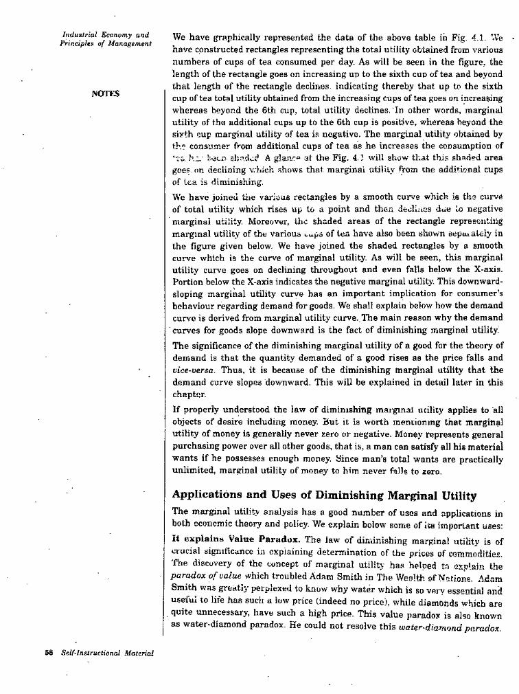
Industrial Econvmy and Principles of Management We have graphically represented the data of the above table in Fig. 4.1. We •
have constructed rectangles representing the total utility obtained from various numbers of cups of tea consumed per day. As will be seen in the figure, the length of the rectangle goes on increasing un to the sixth cud of tea and beyond that length of the rectangle declines indicating thereby that up to the sixth cup of tea total utility obtained from the increasing cups of tea goes on increasing whereas beyond the 6th cup, total utility declines. In other words, marginal utility of the additional cups up to the 6th cup is positive, whereas beyond the sixth cup marginal utility of tea is negative. The marginal utility obtained by th? consumer from additional cups of tea as he increases the consumption of ‘•'i* h.'_ r-ecr- sbn.dud A glan.c“ at the Fig. 4.1 will show that this shaded area goes, on declining v,-hich shows that marginal utility from the additional cups of tea is diminishing.W'e have joined tiie various rectangles by a smooth curve which is tlio curve of total utility which rises up to a point and then decluies due to negative
' marginal utility. Moreover, the shaded areas of the rectangle repreesntillg marginal utility of the various of tea have also been shown sepuialely in the figure given below. We have joined the shaded rectar^les by a smooth curve which is the curve of marginal utility. As will be seen, this marginal utility curve goes on declining throughout and even falls below the X-axis. Portion below the X-axis indicates the negative marginal utility. This downward- sloping marginal utility curye has an important implication for consumer’s behaviour regarding demand for goods. We shall explain below how the demand curve is derived from marginal utility curve.,The main reason why the demand
■ curves for goods slope downward is the fact of diminishing marginal utility. The significance of the diminishing marginal utility of a good for the theory of demand is that the quantity demanded of a good rises as the price falls and vice-versa. Thus, it is because of the diminishing marginal utility that the demand curve slopes downward. This will be explained in detail later in this chapter.If properly understood the law of diminishing marginal utility applies to all objects of desire including money. But it is worth meniionmg that marginal utility of money is generally never zero or negative. Money represents general purchasing power over all other goods, that is, a man can satisfy all his material wants if he possesses enough money. Since man’s total wants are practically unlimited, marginal utility of money to him never falls to zero.
NOTES
Applications and Uses of Diminishing Marginal UtilityThe marginal utility analysis has a good number of uses and applications in both economic theory and policy. We explain bolow some of its important uses:
it explains Value Paradox. The law of diminishing marginal utility is of crucial significance in explaining determination of the prices of commodities. The discovery of the concept of marginal utility has helped to explain the paradox of value which troubled Adam Smith in The Weglth of NKtione. Adam Smith was greatly perplexed to know why water which is so very essential and useful to life has sucii a low price (indeed no price), while diamonds which quite unnecessary, have such a high price. This value paradox is also known as water-diamond paradox. He could not resolve this water-diamond paradox.
are
68 Self-Instructional Material
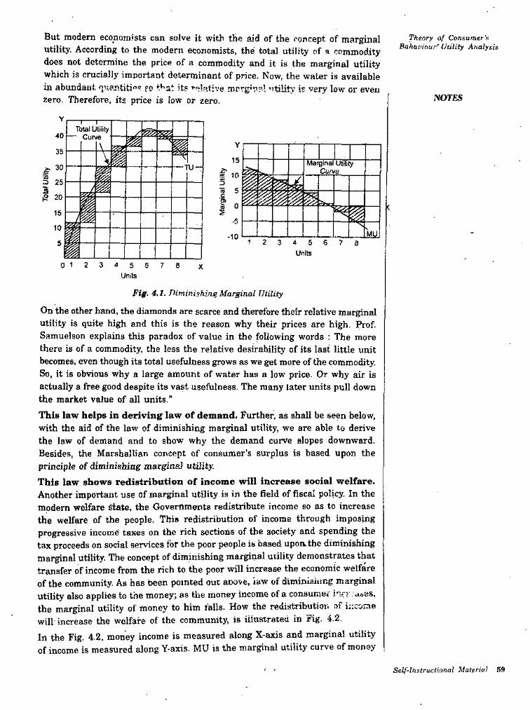
But modem economists can solve it with the aid of the concept of marginal utility. According to the modern economists, the total utility of a commodity does not determine the price of a commodity and it is the marginal utility which is crucially important determinant of price. Now, the water is available in abundant fo it? ’•°!at:ve !nprg>n?l utility i-f very low or evenzero. Therefore, its price is low or zero.
Theory of Consumer's Bahai'iour' Utility Analysis
NOTES
Ititat Utility ■ Curve40 m y\
15 Marginal UtilityCurvele 30
D 25
TU"m f 10
S 5
sDm3
^ 20 m S 0 ;'5116-5
10MU-10
1 2 3 4 5 6 7 8Unitsm
012345678 XUnits
Fig. 4.1. Diminishing Marginal Utility
On the other hand, the diamonds are scarce and therefore their relative marginal utility is quite high and this is the reason why their prices are high. Prof. Samuelson explains this paradox of value in the following words : The more there is of a commodity, the less the relative desirability of its last little unit becomes, even though its total usefulness grows as we get more of the commodity. So, it is obvious why a large amount of water has a low price. Or why air is actually a free good despite its vast usefulness. The many later units pull down the market value of ail units.”This law helps in deriving law of demand. Purther, as shall be seen below, with the aid of the law of diminishing marginal utility, we are able to derive the law of demand and to show why the demand curve slopes downward. Besides, the Marshallian concept of consumer's surplus is based upon the principle of diminishing marginal utility.This law shows redistribution of income will increase social welfare.Another important use Of marginal utility is in the field of fiscal policy. In the modern welfare §tate. the Governments redistribute income so as to increase the welfare of the people. This redistribution of income through imposing progressive income taxes on the rich sections of the society and spending the tax proceeds on social services for the poor people is based upon the diminishing marginal utility. The concept of diminishing marginal utility demonstrates that transfer of income from the rich to the poor will increase the economic welfare of the community. As has been pointed out anove, law uf diminisinng marginal utility also applies to the money; as the money income of a consumer iner aoes, the marginal utility of money to him falls. How the redistributior. of iiicome will increase the welfare of the community, is illustrated in Pig. 4.2.In the Fig. 4-2, money income is measured along X-axis and marginal utility of income is measured along Y-axis. MU is the marginal utility curve of money
Setf-Instruclional Material
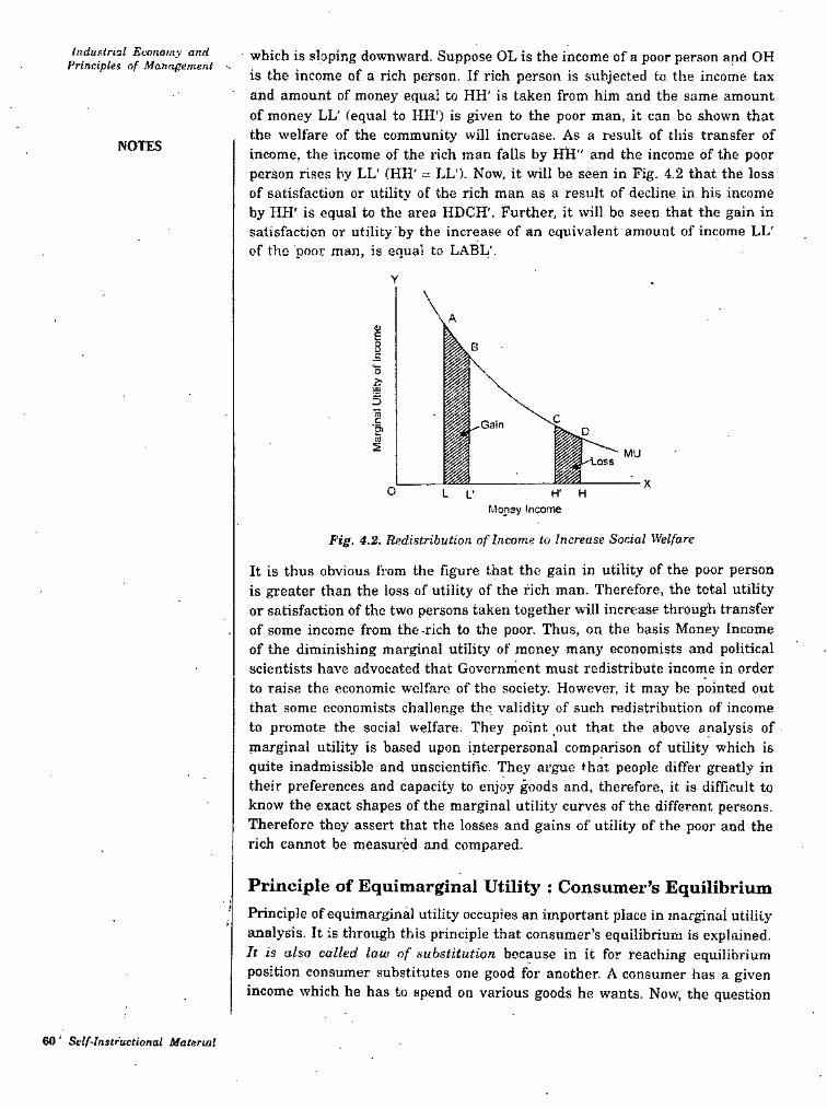
Industrial Eixiitomy and Principles of Management -•
which is sloping downward. Suppose OL is the income of a poor person and OH is the income of a rich person, If rich person is subjected to. the income tax and amount of money equal to HH' is taken from him and the same amount of money LL' (equal to HH') is given to the poor man, it can bo shown that the welfare of the community will increase. As a result of this transfer of income, the income of the rich man falls by HH” and the income of the poor person rises by LL' (HH' = LL’). Now, it will be seen in Fig. 4.2 that the loss of satisfaction or utility of the rich man as a result of decline in his income by HH' is equal to the area HDCH'. Further, it will bo seen that the gain in satisfaction or utility by the increase of an equivalent amount of income LL' of the poor man, is equal to LABL'.
NOTES
A£8o i3g
1m
o L L’ H' HMonsy Iftcome
Fig. 4.2. Redistribution of Income to Increase Social Welfare
It is thus obvious from the figure that the gain in utility of the poor person is greater than the loss of utility of the rich man. Therefore, the total utility or satisfaction of the two persons taken together will increase through transfer of some income from the-rich to the poor. Thus, on the basis Money Income of the diminishing marginal utility of money many economists and political scientists have advocated that Government must redistribute income in order to raise the economic welfare of the society. However, it may be pointed out that some economists challenge the validity of such redistribution of income to promote the social welfare. They point out that the above analysis of marginal utility is based upon interpersonal comparison of utility which is quite inadmissible and unscientific. They argue that people differ greatly in their preferences and capacity to enjoy goods and, therefore, it is difficult to know the exact shapes of the marginal utility curves of the different persons. Therefore they assert that the losses and gains of utility of the poor and the rich cannot be measured and compared.
Principle of Equimarginal Utility : Consumer’s EquilibriumPrinciple of equimarginal utility occupies an important place in marginal utility analysis. It is through this principle that consumer’s equilibrium is explained. It is also called law of substitution because in it for reaching equilibrium position consumer substitutes one good for another. A consumer has a given income which he has to spend on various goods he wants. Now, the question
f
i
60 ‘ Self-Instructional Material
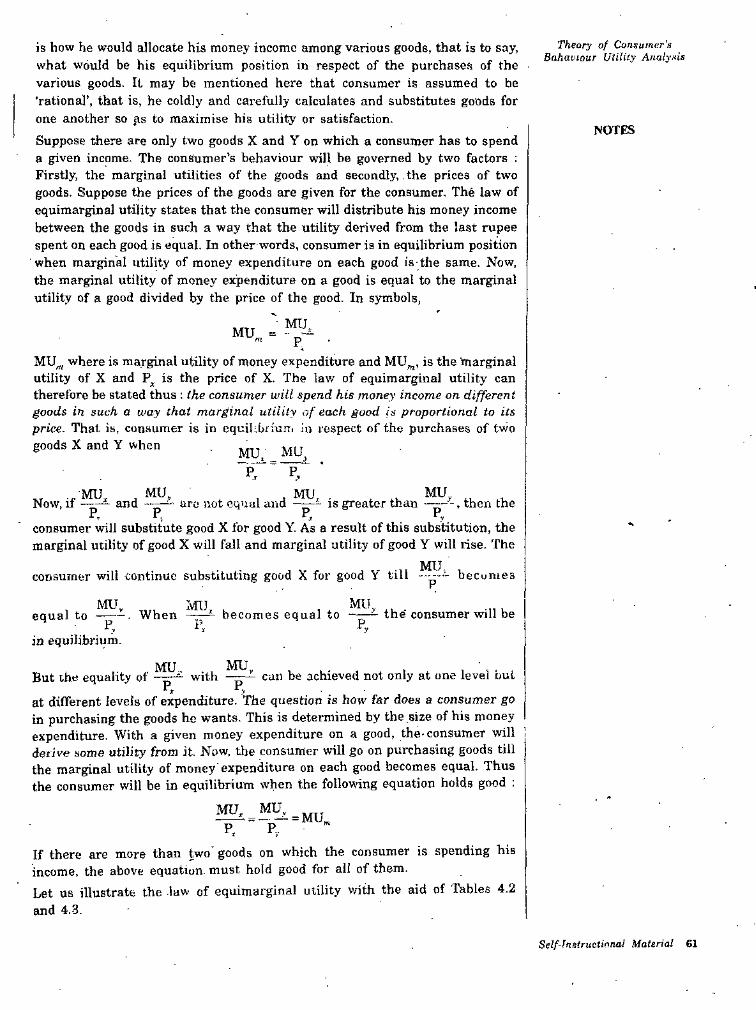
Theory of Consumer's Bahaviour Utility Analysis
is how he would allocate his money income among various goods, that is to say, what would be his equilibrium position in respect of the purchases of the various goods. It may be mentioned here that consumer is assumed to be ‘rational’, that is, he coldly and carefully calculates and substitutes goods for one another so ets to maximise his utility or satisfaction.Suppose there are only two goods X and Y on which a consumer has to spend a given income. The consumer’s behaviour will be governed by two factors : Firstly, the marginal utilities of the goods and secondly,. the prices of two goods. Suppose the prices of the goods are given for the consumer. The law of equimarginal utility states that the consumer will distribute his money income between the goods in such a way that the utility derived from the last rupee spent on each good is equal. In other words, consumer is in equilibrium position when marginal utility of money expenditure on each good is the same. Now, the marginal utility of money expenditure on a good is equal to the marginal utility of a good divided by the price of the good. In symbols,
NOTES
Ml^P. ■
MU^ where is marginal utility of money expenditure and MU,„, is the marginal utility of X and is the price of X. The law of equimarginal utility can therefore be stated thus : the consumer will spend his money income on different goods in such a way that marginal utility of each good is proportional to its
MU =m
price. That is, consumer is in equihbiiuni in respect of the purchases of two goods X and Y when MUMU.
P P^.r ‘■s
Now, if and are not equal and is greater than —.t
consumer will substitute good X for good Y. As a result of this substitution, the marginal utility of good X will fall and marginal utility of good Y will rise. The
becunies
MU,, then the
MU,consumer will continue substituting good X for good Y till --
......... , , MU,—- becomes equal to —
P1.equal to —
in equilibrium.
:\fu the' consumer will be. When
But the equality of achieved not only at one level but
at different levels of expenditure. The question is how far does a consumer go in purchasing the goods he wants. This is determined by the size of his money expenditure. With a given money expenditure on a good, the-consumer will derive some utility from it. Now. the consumer will go on purchasing goods till the marginal utility of money'expenditure on the consumer will be in equilibrium when the following equation holds good :
MU, MU,- --=MU„
each good becomes equal. Thus
Pvp.If there are more than two' goods on which the consumer is spending his income, the above equation, must hold good for all of them.Let us illustrate the law of equimarginal utility v/ith the aid of Tables 4.2 and 4.3.
Self-tnsiructionai Material 61
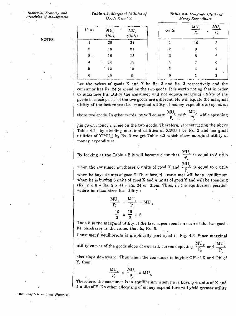
tndiistriol Economy and Principles of Management
Table 4.2. Marginal UHlilies of Goods X and Y. -
Table 4.3, Marginal Utility of Money Expenditure..
MU,MU,Units Mb\ MU\
(Utils) (Utils)Units P. P,
NOTES 1 20 24 1 10 82 718 21 2 93 16 18 3 8 64 14 4.15 7 5
' 125 12 5 6 46 0 5 310
Let the prices nf goods X and Y be Rs. 2 and Rs. 3 respectively and the consumer has Rs. 24 to spend on the two goods. It is worth noting that in order to maximise his utility the consumer will not equate marginat utility of the goods because prices of the two goods are different. He will equate the marginal utility of the last rupee (i.e., marginal utility of money expenditure) spent on
these two goods. In other words, he will equate ——
his given money income on the two goods. Therefore, reconstructing the above Table 4.2 by dividing marginal utilities of XiMU,) by Rs, 2 and marginal utilities of YfMU^) by Rs. 3 we get Table 4.3 which show marginal utility of money expenditure.
MU—while spending Py
with
By looking at the Table 4.2 it will become clear that
, MU,when the consumer purchases 6 units of good X and
Pywhen he buys 4 units of good Y. Therefore, the consumer will be in equilibrium when he is buying 6 units of good X and 4 units of good Y and will be spending (Rs. 2x6 + Rs. 3x4) = Rs. 24 on them. Thus, in the equilibrium position where he maximizes his utility : '
is equal to 5 utils
is equal to 5 utils
MU,MU,p m—
P,10 . 15
T = ^Thus 5 is the marginal utility of the last rupee spent on each of the two goods he purchases is the same, that is, Rs, 5.Consumers’ equilibrium is graphically portrayed in Fig. 4.3. Since marginal
MUutility curves of the goods slope downward, curves depicting —^
VT
also slope downward. Thus when the consumer is buying OH of X and OK of Y, then
2
MU,and
P\
MU.MU,= MU.„
Therefore, the consumer is in equilibrium when he is buying 6 units of X and 4 units ofY. No other allocating of money expenditure will yield greater utility
=:- P>
62 ■ Self-Instructional Mareriat
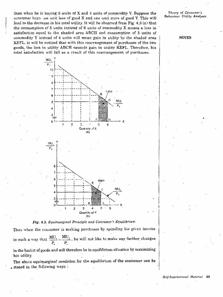
Theory of Consumer's Bahaviour Utility Analysis
than when he is buj'ing 6 units of X and d units of commodity Y. Suppose the confiuiner buys .’fie unit less of good X and one unit more of good Y. This will lead to the decrease in bis total utility. It wj]] be observed from Fig, 4,3 (n) that the consumption of 5 units instead of 6 units of commodity X means a loss in satisfaction equal to the shaded area ABCH and consumption of 5 units of commodit}’ Y instead of 4 units will mean gain in utility by the shaded area KEFL. it will be noticed that with this rearrangement of purchases of the two goods, the loss in utility ABCH exceeds gain in utility KEFL. Therefore, his total satisfaction will .fall as a result of this rearrangement of purchases.
NOTES
YMU,P,
IP
■ 9
B
^ A7 K ►Loss
6 A
MU,5P.4
30AM H0.'- X
1 2 Q 5Quatmty ,>f X
ta)
MU^P)'
6
7
6 Gain/5
4
3 ju
K02 3 4 5 61
Quanfily of V(bj
Fig- 4.3. Equimarginal Principle and. Consumer’s Equilibrium
Thus whe-n the consumer is making purchases by spending his given income
= . he will not like to make anv further changesP.
in such a way thatP,
in the basket of goods and will therefore be iu equilibriuni situation by maximizing his utility. . . 'The above equimarginal condition for the equilibrium of the consumer can be
, stated ill the following ways ;
Self-Instructional Material 63
Industrial Economy and Principles of Management
A consumer is in equilibrium when he equalises the ratios of marginal utilities of goods and their prices with each other. In other words,
MU, _MU^P P ^* ar J* ^
MU„he is in equilibrium when « MU„,
NOTESBy rearranging the above equation we find that a consumer is in equilibrium when he equalises the ratio of marginal utilities of goods with the ratio of corresponding prices for each pair of goods consumed.
-----= andMU, P,MU.-----measure the marginal utility of a rupee's worth
P,
of each good consumed at the given price, consumer can be said to be in equilibrium when the marginal utility of the last rupee spent on each good purchased is equal. Marginal utility of the last rupee spent on a good means the marginal utility of a rupee’s worth of the good. Thus, consumer is equilibrium when he spends his given income on various commodities in such a way that utility from the last rupee spent on each good is the same. If the marginal utility of the last rupee spent on each good is denoted by MU„^, then equilibrium condition of consumer’s equilibrium can also be stated as under :
MU, MU, MU,■P. ^P. ^ P.
Ui)-
MU, P, j-----= — and so forth.MU, P,
that is, when
MiJ.- -— or• (iii) Since
= MU,„
Derivation of the Demand Curve and the Law of DemandWe now turn to explain how the demand curve and the law of demand is derived in the cardinal utility analysis. As stated' above, the demand curve or the law of demand shows the relationship between price of a good and its quantity demanded. Marshall derived the demand curves for goods from their utility functions. It should be further noted that in his cardinal utility analysis of demand Marshall assumed the utility functions of different goods to be independent of each other. In other words. Marshallian technique of deriving demand curves for the goods from their utility functions rests on the hypothesis of additive utility functions, that is, utility functions of each good consumed by a consumer does not depend on the quantity consumed of any other good. As has already been noted that in case of independent utilities or additive utility functions, the relations of substitution and complementarily between goods are ruled out. Further, in deriving a demand curve or law of demand Marshall assumes that marginal utility of money to remain constant. The law of demand or the demand curve can be derived in two ways : first, with the aid of law of diminishing marginal utility, and secondly, with the help of the law of equimarginal utility. We shall explain below these two ways of deriving the demand curve and the law of demand.Derivation of Demand Curve from Law of Diminishing Mai^nal Utility.In order to derive the demand curve (and accordingly law of demand) measure marginal utility of a good in terms of money (i.e., in terms of rupees! as Marshall did. Measuring marginal utility in terms of money or rupees implies how much value in terms of rupees an individual places on the successive units of the commodity consumed. In other words, how much money a consumer
we
64 Self-Instructional Material
Theory of Consumer's fiaAoutemr Ulility Analynis
is prepared to pay for a unit of commodity will measure the marginal utility of that unit of the commodity, in terms of money.The law of marginal utility states that as the quantity of a good with a consumer increases, marginal utility of the good to him falls. In other words, the marginal utility curve of a good is downward sloping. Now, a consumer will go on purchasing a good until the marginal utility of the good pouals the market price. In other words, the consumer will be in equilibrium in respect of the quantity of the good purchased where marginal utility of the good equals its price. His satisfaction will he maximum only when marginal utility equals price. Thus the “marginal utility equals price” is the condition of equilibrium. When the price of the good falls, downward-sloping marginal utility curve implies that the consumer must buy more of the good so that its marginal utility falls and becomes equal to the now price, It therefore follows that the diminishing marginal utility curve of a good implies the downward-sloping demand curve, that is. as the price of the good falls, more-of it will be bought.The whole argument will be more clearly understood firom Fig. 4.4. In panel (a) of Fig. 4.4 the curve MU represents the diminishing marginal utility of the good measured in terms of money. In pane! (i) of Fig. 4.4-we measure price on the Y-axis, Suppose the price of the good is OP^. At this price the consumer will be in equilibrium when he purchases Oqj quantity of the goods since at Og, the marginal utility of good X equal to MUj is equal to the given price OPj. Now, if the price of the good falls to OPj, the equality between the marginal utility and the price will be disturbed. Marginal utility MU, from good X at the quantity Og, will be greater than the new price OPj- In order to equate the marginal utility with the lower price OPg, the consumer mustibuy more of the good. It is evident from Pig. 4.4 that when the consumer increases the quantity purchased to Oq^ the marginal utility of the good falls to MU2 and becomes equal to the new price OP2. Hence, at price OPj. consumer demands Oq2 amount of the commodity. Further, if the price falls to OP3, this is equal to the marginal utility MU3 of the good at the larger quantity Ogj. Thus at price OP3, the consumer will demand Ogj quantity of the good X. It is in this way the downward-sloping marginal utility curve is transformed into the downward- sloping demand curve when we measure marginal utility of a good in terms of money. It is worth noting that negative segment of the marginal utility curve MU., will not constitute a part of the demand curve. This is because no rational consumer will buy any further units of the commodity which reduces his total utility and make marginal utilities negative.
NOTES
MUx DDemand CurveIMarginal Utility Curve
'Si CLD« MUi ^ MUj
Pi
P2
MU3 P3MU>,
£.xo odl d2 '33 Quantity of X
ai 02 Q3Quantity of X
(8) (b)
Fig. 4.4. Derivation of Demand Curve in Marshallian Cardinal Utility Analysis
Self Instructional Material 65
Industrial Economy and Principles of Management
It is thus clear that when the price of the good falls, the consumer buys more of the good so as to equate its marginal utility to the lower price. It follows thurefove that the quantity demandod of a good varies inversely with price; the quantity rises when the price falls and vice-versa, other things remaining the sarue. This is the famous Marshallian Law of Demand. It is quite evident that the law of demand is directly derived from the law of diminishing marginal utility. The downward-sloping marginal utility curve is transformed into the downward-sloping demand curve. It follows therefore that the force working behind the law of demand or the demand curve is the forte of dimiih-^hing marginal utility.Derivation of Law of Demand : Multi-Commodity Model. We now proceed to derive the law of demand and the nature of the demand curve from the principle of equimarginal utility.in case when a consumer spends his money income on more than one commodity. Consider the case of a consumer who has a certain given income to spend on a number of goods. According to the law of equimarginal utility, the consumer is in equilibrium in regard to his purchases of various goods when marginal utilities of the goods are proportional to their prices. Thus, the consumer is in equilibrium when he is buying the quantities of the two goods in such a way that satisfies the following proportionality rule :
NOTES
MU, MU,P. " P.
where stands for marginal utility of money expenditure. Thus, in theequilibrium position, according to the above principle of equimarginal utility, the ratios of the marginal utility and the price of each commodity a consumer buys will equal the marginal utility of the last rupee spent on each g^od. It
MU,follows therefore that a rational consumer will equalise "p of good X "'ith
MU, = MU„P.
MUof good Y and so on.
Given that other things such tastes and proferenees of o censumer, his in..cme, prices of other related commodities remain constant, we consider the demand for good X. Assume the price of good X is equal to P,. The consumer will allocate his given money income on various goods he purchases so that
MU, MU^p. ^ n
With the fall in the price of good X, the price of good Y. consumer's income
and his tastes remaining unchanged, the equality of MHi. or with MUP, Py
in general would be disturbed. With lower price of good X than before,____ ‘Pi
> MU,„
= MU„, and so forth. Let us suppose that price of good X falls.
MU
PMU.
. (It is of course assumed that marginal utility of money expenditureor p
in general fMU,„) does not change as a result of the change iii the priLc of one good). Then, in order to restore the equality, marginal utility of good X has to be reduced which can be done only if consumer buys more of good X. It is thus clear from the equimarginal principle that as the price of a good falls, its quantity demanded will rise, other things remaining the same. This proves the
66 Hdf-Instructional Material
law of demand which states that there is inverse relationship between price of a good and its quantity demanded. The operation of this law of demand makes the demand curve downward sloping.
Thenry of Consumer's Bahauiour Utility Analysis
Limitations of the Law of Equimarginal UtilityLike other laws of economics, law of equimarginal utility is also subject to various limitations. This law, like other laws of economics, brings out an important tendency among the people. This is not necessary that all people exactly follow tliis law in the allocation of their money income and therefore all may not obtain maximum satisfaction. This is due to the following reasons:
1. For applying this law of equimarginal utility in the real life, consumer must weigh in his mind the marginal utilities of different commodities. For this he has to calculate and compare the marginal utilities obtained from different commodities. But it has been pointed out that the ordinary consumers are not so rational and calculating. Consumers are generally governed by habits and customs. Because of their habits and customs they purchase particular amounts of different commodities, regardless of whether the pai-ticular allocation maximizes their satisfaction or not.
2. For applying this law in actual life and equate the marginal utility of rupee obtained from different commodities, the consumers must be able to measure the marginal utilities of different commodities in cardinal terms. However, this is easier said than done. It has been said that it is not possible for the consumer to measure the utility cardinally. Being a state of feeling and also there being no objective units with which to measure utility, it is cardinally immeasurable. It is because the immeasurability of utility in cardinal terms that consumer’s behaviour has been explained with the help of ordinal utility by J.R. Hicks and R.G.D. Allen. Ordinal utility analysis involves the use of indifference curves which we shall explain in the next chapter.
3. Another limitation of the law of equimarginal utility is found in case of indivisibility of certain goods. Goods are often available in large indivisible units. Because the goods are indivisible, it is not possible to equate the marginal utility of money spent on them. For instance, in allocating money between the purchase of car and foodgrains, marginal utilities cannot be equated. Car costs about Rs. 20,000 and is indivisible, whereas foodgrains are divisible and money spent on them can be easily varied. Therefore, the marginal utility of rupee •obtained from car cannot be equalised with that obtained from foodgrains. Thus, indivisibility of certain goods is a great obstacle in the way of equalisation of marginal utility of a rupee from different commodities.
Critical Evaluation of Marshall’s Cardinal Utility AnalysisUtility analysis of demand which wc have studied above has been criticised on various grounds. The following shortcomings, and drawbacks of cardinal utility analysis have been pointed out :
1. Cardinal measurability of utility is unrealistic. Cardinal utility analysis of demand is based on the assumption that utility can be measured in absolute, objective and quantitative terms. In other words, it is assumed in this analysis that utility is cardinally measurable. According to this, how much utility a consumer obtains from goods can be
NOTES
Sclf-lnstrur.tional Material 67
Industrial Economy and Principles of Management expressed or stated in cardinal numbers such as 1, 2, 3. 4 and so
forth. But in actual practice utility cannot be measured in such quantitative or cardinal terms. Since utility is a psychic feeling and a subjective thing, it cannot therefore be measured in quantitative terms. In real life, consumers are only able to compare the satisfactions derived from various goods or various combinations of the goods. In other words, in the real life consumer can state only whether a good or a combination of goods gives him more, or less, or equal satisfaction as compared to another. Thus, economists like J.R. Hicks are of the opinion that the assumption of cardinal measurability of utility is unrealistic and therefore it should be given up.
2. Hypothesis of independent utilities is wrong. Utility analysis' also assumes that utilities derived from various goods are independent. This means that the utility which a consumer derives from a good is the function of the quantity of that good and of that good alon^'. In other words, the assumption of independent utilities implies that the utility which a consumer obtains from a good does not depend upon the quantity consumed of other goods; it depends upon the quantity purchased of that good alone- On this assumption, the total utility which a person gets from the whole collection of goods purchased by him is simply the total sum of the separate utilities of the good. In other words, utility function is additive.Neoclassical economists such as Jevons, Menger, Walras and Marshall considered that utility functions were additive. But in the real life this is not so. In actual life the utility or satisfaction derived from a good depends upon the availability of some other goods which may be either substitute for or complementary with it. For example, the utility derived from a pen depends upon whether ink is available or not. On the contrary, if you have only tea. then the utility derived from it would be greater, but if along with tea you also have the coffee then the utility of tea to you would be comparatively less. Whereas pen and ink are complements with each other, tea and coffee are substitutes for each other. It is. thus clear that various goods are related to each other in the sense that some are complements with each other and some are substitutes for each other. As a result of this, the utilities derived from various goods are interdependent, that is, they depend upon each other. Therefore, the utility obtained from a good is not the function of its quantity alone but also depends upon the availability or consumption of other related goods (complements or substitutes). It is thus evident that the assumption of the independence of utilities by Marshall and other supporters of cardinal utility analysis is a great defect and shortcoming of their analysis. As we shall see below, the hypothesis of independent utilities along with the assumption of constant marginal utility of money reduces the validity of Marshallian demand theorem to the one-commodity model only.
3, Assumption of constant cardinal utility of money is not valid. An important assumption of cardinal utility analysis is that when a consiamer spends varying amount on a good or various goods or when the price of a good changes, the marginal utility of money remains unchanged. But in actual practice this is not correct. As a consumer spends his money income on the goods, money income left with him declines. With the decline in money income of the consumer as a result of
NOTES
'68 Self-Instructional Material
increase in his expenditure on goods, the marginal utility of money to him rises. Further, when the price of a commodity changes, the real income of the consumer also changes. With this change in real income, marginal utility of money will change and this would have an' effect, on the demand for the good in question, even though the total money income available'with the consumer remains the same. But utility analysis ignores all this and does not take cognizance of the changes in real income and its effect on demand for goods following a change in the price of a good.As we shall see below, it is because of assuming constant marginal utility of money that Marshall ignored the income effect of the price change and this prevented Marshall from understanding the composite character of the price effect (that is, price effect being sum of substitution effect and income effect). Moreover, as shall be seen later,'the assumption of constant marginal utility of money together with the hypothesis of independent utilities, renders the Marshall’s demand theorem to be valid in case of one commodity only. Further, it is because of the constant marginal utility of money and therefore the neglect of the income effect by Marshall that he could not explain Ciffen Paradox.As has been explained earlier, according to Marshall, utility from a good can be measured in terms of money (that is, how much money a consumer is prepared to sacrifice for a good). But, to be able to measure utility in terms of money, marginal utility of money itself should remain constant. Therefore, assumption of constant marginal utility of money is very crucial in Marshallian demand analysis. On the basis of constant marginal utility of money Marshall could assert that “utility is not only” measurable in principle but also “measurable in fact”. But. as we shall see below, in case consumer has to spread his money income on a number of goods, there is a necessity for revision of marginal utility of money with every change in the price of a good. In other words, in a multi-commodity model marginal , utility of money does not remain invariant or constant. Now, when it is realised that marginal utility of money does not remain constant, then Marshall’s belief that utility is measurable in fact in terms of money does not hold good. However, if in marginal utility analysis, utility is conceived only to be measurable in principle and not in fact, then it practically gives up cardinal measurement.of utility and comes near the ordinal measurement of utility.
4. Marshallian demand theorem cannot genuinely be derived except in a one commodity case. J.R. Hicks and Tapas Majumdar have further criticised the Marshallian utility analysis on the ground that “Marshallian demand theorem cannot genuinely be derived from the marginal utility hypothesis except in a one-commodity model without contradicting the assumption of constant marginal utility of money.” In other words, Marshall's demand theorem and constant marginal utility of money are incompatible except in a one commodity case. As a result, Marshall’s demand tlieorem cannot be validly derived in the case when a consumer spends his money on more than one good. Thus, we see that marginal utility of money cannot be assumed to remain constant when the consumer has to spread his money income on a number of goods. In case of more than one good, Marshallian demand theorem cannot be
Theory of Consumer’s Bahaviour Utility Analysis
NOTES
Self-Instructional Material &
{iiduslriof Economy and Principles of Management genuineJy derived whiie keeping the marginal utility of money constant,
if, in Ivlarshallian demand analysis, this difficulty is avoided “by.giving up the assumption of constant marginal utility of money, then money can no longer provide the measuring rod, and we can no longer express uio marginal utility of a commodity in units of money. If we caiuioc expreatJ marginal utility in terms of common numeraire (which money is defined to fag), the cardinality of utility would be devoid of any operational significance.”
5 Cardinal utility analysis does not split up the price effect into substitution and income effects. The third shortcoming of the cardinal utility . analysis is that it does not distinguish between the income effect and the suhstiiulion effect of the price change. vVe know that when the price of a good falls, the consumer becomes betm.' off than before, that is, a fall in price of a good brings about an increase in the real income of the consumer. In other words, if with the fall in price the consumer purchases the same quantity of the good as before, then he would be left with some income. With this income he would be in a position to purchase more of this good as well as other goods. This is the income effect of the fall in price on the quantity demanded of a good. Besides, when the price of a good falls, it becomes relatively cheaper than other goods and as a result the consumer is induced to substitute that good for others. This results in the increase in the quantity demanded of that good. This is the substitution effect of the price change on the quantity demanded of the good.With the fall in price of a normal good, the quantity demanded of*' rises because of income effect and substitution effect. But marginal utility analysis does not make clear the distinction between the income and the substitution effects of the price change. In fact. Marshal! and other exponents of cardinal utility analysis ignored income effect of the price change by assuming the constancy of marginal utility of money. Thus, ir.g'ginal utility analysis does not tell us about how much quantity demanded increases due to income effect and how much due to substitution effect as a result cf the fall in price of a good. J.R. Hicks rightly remarks, “that distinction between income effect and substitution effect of a price change is accordingly left by the cardinal theory as an empty box which is crying out to be filled."
6. Marshall could noi explain Giffcn Paradox. By not visualising the price effect as a combination of substitution and income effects and ignoring the income effect of the price change, Marshall could not explain Giffen Paradox. He treated it merely as an exception to his law of demand. In constant to it, indifference curves analysis has been able co explain satisfactorily the Giffen good case. According to indiffo-cnce carves analysis, in case of Giffen Paradox or Giffen good
. negative income effect of the price change is more powerful than the substitution effect so, that when the price of a Giffen good falls the negative income effect outweighs the substitution effect with the result that quantity demanded of it falls. Thu.s, in case of a Giffen
qnan'-ity dem-r.nded varies directly with the price and the Marshall’s aw of d-’Tnand does not hold good. It is because of tire constant
marginal utility of money and therefore the neglect of the income effect of price change that Marshall could not explain why the quantity demanded of a Giffen good falls when its price falls, and rises when
N01ES
1
70 Self-instructional Material
Thforv of Consumer's Bahaviour Utility Analysisits price rises. This is a seriniis lanma in Marshallian’s utility analysis
of demand.7. Cardinal utility analysis assumes too much and exolains too Utile.
Cardinal utility analysis xs also criticised on the ground that it takes mere a.ssnmpiions .ond aho more restrictive ones than these of ordinal utility aiialysis of indifference curvms technique. Cardinal utility analysis assumes, among others, that utility is cardinally measurable and also that marginal utility of money remains constant. Hicks-Allen’s indifference curve analysis does not take thess assumprions and even then it is not only able to deduce ail the theorems which cardinal utility analy.sis can but also ueuuces u more f^enei ul theorem of demand. In ocher words, indifference curve analysis explains not only that much as cardina! utility o.nn!y?is but even goes further and that too wjth fo,i;or and le'^s reri-rictive assumption?. Taking less rectriotive a.csumption of ordinal measurement of utihey and without assuming constant fuargiaai utiuty of money, indifiei ence curve analysis is aoie to arrive at the condition of consumer’s equilibrium, namely, equality of marginal
,rate of substituticn (MRS) with the price ratio between the goods, vvh’.ch is rimilar to the nroportionality rule of Marshnll. Fiirtber, since inniffeience curve analysis does not assume constant marginal ui-ilily of iiionej, ic is able to deiive a valid demand theorem in a more tlian one commodity case. .Iv shall, be explained in the next chapter that indifference curve oiittlysis is able to explain Giffea Paradox wliich mai'shau with his cardinal utility analysis could not. In other words, indifference curve analysis clo^r'y explains '.vby in rase ofGif^on goods, quanhty demanded
’ ’ncreasr? with *.he rise in price and dec.fc.a5c5 wiH'. th^ fall in price. Indifference cu.rve analysis explains even the case of ordinary inferior goods (other than Giffer. goods) in a more on«'ytical manner. It may be noted that even if the valid demand theorem could be derived from the Marshallian hypothesis, it would still be rejected because "bstter kypoikesis" cf indifference praforenco analysis was available vih-nh -c’' evunriatp ^ more "-rern' dev'.'''vd ibr-yrom (covering the case of Gitfen goods) with fewer, less restrictive and more realistic assumptions.Becausp of’■he above draw'backs, bopri gi->’en upin modern economic theory and tlemana is analysed with mdilference Curves which we sliaii explain in the next unit.
NOTES
Self-Jnsln'riional Material 71
Industrial Economy and Principles of Management
STUDENT ACTIVITY
1. Define the terms ‘utility’, ‘total utility” and ’marginal utility’. What are the assumptions of Marginal utility analysis ?
2. State and illustrate the law of diminishing marginal utility with the help of a suitable example.
72 Self-Instructional Material
Theory of Consumer'^ Bahaviour Utility AnalysisSUMMARY
• Marginal utility of a commodity to a consumer is the extra utility which he gets when he consumes one more unit of the commodity.
• ■ The exponents of a cardiT»al utility theory or what is also called marginalutility analysis regards utility to be a cardinal concept.
• “If money is supposed to provide the measuring rod of utility, then evidently as with all measuring rods, its unit must be invariant: it must measure the same amount of utility in all circumstances.”
• An important tenet of marginal utility analysis relates to the behaviour of marginal utility.
• The significance of the diminishing marginal utility of a good for the theory of demand is that the quantity demanded of a good rises as the price falls and vice-versa.
• The law of diminishing marginal utility is of crucial significance in explaining determination of the prices of commodities.
NOTES
REVIEW EXERCISES1. Explain the law of diminishing maigfinal utilily and discuss its limitations.2. How does consumer obtain equilibrium under the law of equi-maiginal
utility ? Discuss.3. State the essence of law of Diminishing Marginal Utility.
Self-Instructional Material 78
Industrial Economy and Principles of Manageme.n' UNIT 5 CONSUMER SURPLUS
NOTES
□ Meaning or Goiisumer Surplus□ Uses and Applications of Consumer Surplus
MEA^mG OF CONSLTMFR STJP.PI.USThe concept of consumer surplus was first formulated by Dupuit in 1844 to measure social benefits of public goods such as canals, bridges, national highways. Marshall further refined and popularised this in his 'Principles of Economics’ published in IbiiO. The cvnccpi of consumer surplus became the basis of old welfare economics. Marshall’s concept of consumer’s surplus was based on,the cardinal measurability and interpersonal comparisons of utility. According to him. every increase in tlic 'c is aii indicator of the increasein social welfare. As v”« chajl difference between the price that one is willing to pay’ and The price one actually pays’ m'- a particular product.
hpiow, cons'imer’s surplus is simply the
r cuiisuiner’s surplus is a viry important concept in economic theory,Concuplespecially in theory of demand and welfare economics. This concept is important • not only in economic theory but also in economic policies such as taxation by the Government and price policy pursued by the monopblistic seller of a product. Tho essence of the concept of consumer's surplus is that a consumer derives extra satisfaction from the purchases he daily makes over the price he actually pays for them. In other words, people generally get more utility from theconsumption of goods than the prico they actually pay for them. It has been found that people are prepared to pay more pries for the goods than they actually pay for them. This extra satisfaction which the consumers obtain from buying a good has been called consumer surplus. Thus, Marshall defines the consumer's surplus in tho following words: '‘erress of the price which a consumer would be willing to pay rather than go without a thing over that which he actually does pay, is the economic measure of this surplus satisfaction....it may be called consumer's surplus.”The amount of money which a person is willing to pay for a good indicates the amount of utility he derives from that good; the greater the amount of money he is willing to pay, the greater the utility he will obtain from it. Therefore, the marginal utility of a unit of a good determines the price a consumer will be prepared to pay for that unit. The total utility which a person will get from a good will be given by the sum of marginal utilities fXMI) of the units of a good purchased and tho total price which he actually pays is equal to the price per unit of the good multiplied by tho number of units it purchased. Thus :Consumer’s surplus =W’hat a consumer is willing to pay minus what he actually
pays.
= I Marginal utility - (Price X Nu.mber of units of a commodity-purchased)
74 Self-!nsrrucliv‘t(.ii i’liiic.riol
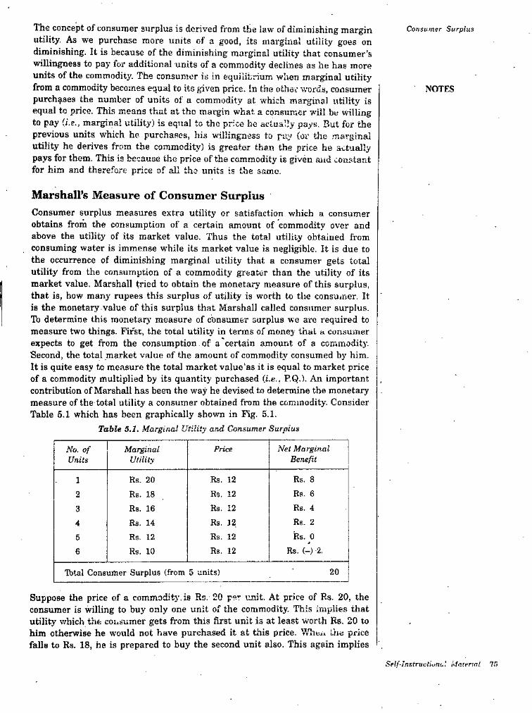
The concept of consumer surplus is derived from the law of diminishing margin utility. As we purchase more units of a good, its marginal utility goes on diminishing. It is because of the diminishing marginal utility that consumer’s willingness to pay for additional units of a commodity declines as he has units of the commodity. The consumer is in equilibrium when marginal utility from a commodity becomes equal to its given price. In the other words, consumer purchases the number of units of a commodity at which marginal utility is equal to price. This means that at the margin what a consumer will be willing to pay ii.e., marginal utility) is equal to the price be actually pays. But for the previous units which he. purchases, his willingness to pay (ov the .marginal utility he derives from the commodity) is greater than the price he actually pays for them. This is because the price of the commodity is given aiid constant for him and therefore price of all the units is the same.
Consumer Surplus
more
NOTES
Marshall’s Measure of Consumer SurplusConsumer surplus measures extra utility or satisfaction which a consumer obtains from the consumption of a certain amount of commodity over and above the utility of its market value. Thus the total utility obtained from consuming water is immense while its market value is negligible. It is due to the occurrence of diminishing marginal utility that a consumer gets total utility from the consumption of a commodity greater tlian the utility of its market value, Marshall tried to obtain the monetary measure of this surplus, that is, how many rupees this surplus of utility is worth to the consuiner. It is the monetary-value of this surplus that Marshall called consumer surplus. To determine this monetary measure of consumer surplus wo are required to measure two things. First, the total utility in terms of money that a consumer expects to get from the consumption. of a certain amount of a commodity. Second, the total market value of the amount of commodity consumed by him. It is quite easy to measure the total market value‘as it is equal to market price of a commodity multiplied by its quantity purchased (Le., P.Q.). An important contribution of Marshall has been the way he devised to determine the monetary measure of the total utility a consumer obtained from the commodity. Consider Table 5.1 which has been graphically shown in Fig. 5.1.
Table 5.1. Marginal Utility and Consumer Surplus
Net Marginal Benefit
No. of Units
MarginalUtility
Price
Rs. 8Rs. 20 Rs, 121Rs. 6 Rs. 4
Rb- 18 Rb. 16
Rs. 12 Rs. 12
23
Rs. 2 Rs. 0
j
Rs, (-) 2,
Rs. 12Rs, 144Rs. 12Rs. 12
Rb. 105
Rs. 126
20Tbtal Consumer Surplus (from 5 units)
Suppose the price of a commodity.is Rs. 20 per i.init. At price of Rs. 20, the consumer is willing to buy only one unit of the commodity. This implies that utility v/hich the consumer gets from this first unit is at least worth Ks. 20 to him otherwise he would not have purchased it at this price. 'ATieji trie price falls to Rs. 18, he is prepared to buy the second unit also. This again implies
Self-lnstructMiul Martrin! 7.'i
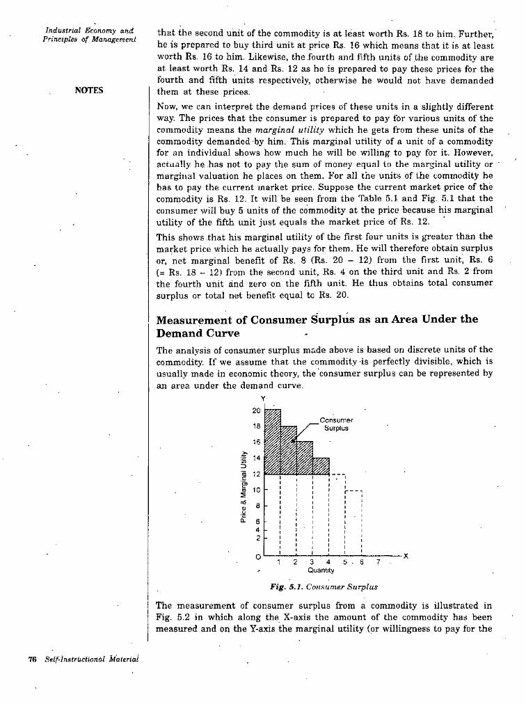
Industrial Economy and Principles of Management that the second unit of the commodity is at least worth Rs, 18 to him. Further,
he is prepared to buy third unit at price Rs. 16 which means that it is at least worth Rs. 16 to him. Likewise, the .fourth and fifth units of the commodity are at least worth Rs. 14 and Rs. 12 as he is prepared to pay these prices for the fourth and fifth units respectively, otherwise he would not have demanded them at these prices.Now, we can interpret the demand prices of these units in a slightly different way. The prices that the consumer is prepared to pay for various units of the commodity means the marginal utility which he gets from these units of the commodity demanded by him. This marginal utility of a unit of a commodity for an individual shows how much he will be willing to pay for it. However, actually he has not to pay the sum of money equal to the marginal utility or marginal valuation he places on them. For all the unite of the commodity he has to pay the current market price. Suppose the current market price of the commodity is Rs. 12. It will be seen from the Table 5.1 and Fig. 5.1 that the consumer will buy 5 units of the commodity at the price because his marginal utility of the fifth unit just equals the market price of Rs. 12.This shows that his marginal utility of the first four units is greater than the market price which he actually pays for them. He will therefore obtain surplus or, net marginal benefit of Rs. 8 (Rs. 20 - 12) from the first unit. Rs. 6 (= Rs. 18 - 12) from the second unit, Rs. 4 on the third unit and Rs. 2 from the fourth unit and zero on the fifth unit. He thus obtains total consumer surplus or total net benefit equal to Rs. 20.
NOTES
Measurement of Consumer Surplus as an Area Under the Demand CurveThe analysis of consumer surplus made above is based on discrete units of the commodity. If we assume that the commodity is perfectly divisible, which is usually made in economic theory, the consumer surplus can be represented by an area under the demand curve.
20Consumer
Surplus18
16
2r 14S3•(5 12c
10n I--------Si6 8S'CCL 6
42
01 2 3 4 6-67.
Quantity
Fig. 5.1. Consumer Surplus
The measurement of consumer surplus from a commodity is illustrated in Fig. 5.2 in which along the X-axis the amount of the commodity has been measured and on the Y-axis the marginal utility (or willingness to pay for the
76 Self-instructional Material
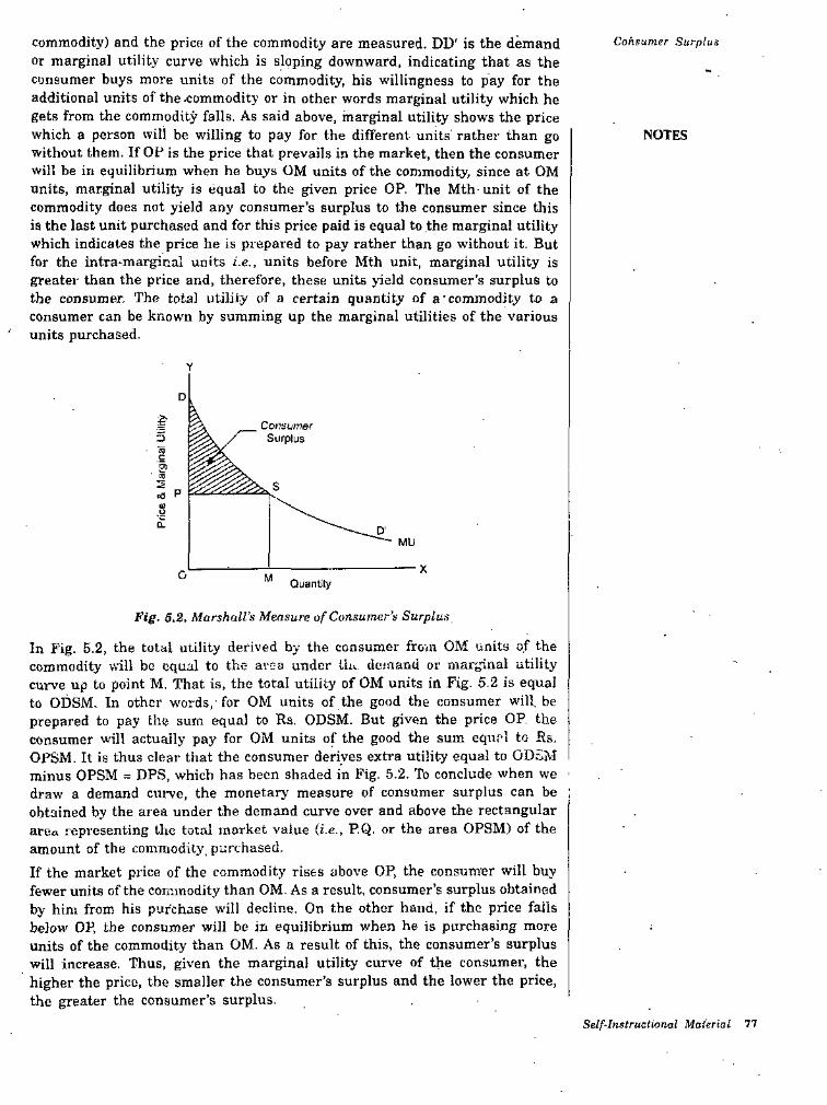
commodity) and the price of the commodity are measured. DD’ is the demand or marginal utility curve which is sloping downward, indicating that as the consumer buys more units of the commodity, his willingness to pay for the additional units of the .commodity or in other words marginal utility which he gets from the commodity falls. As said above, marginal utility shows the price which a person will be willing to pay for the different units rather than go without them. If OF is the price that prevails in the market, then the consumer will be in equilibrium when he buys OM units of the commodity, since at OM units, marginal utility is equal to the given price OP. The Mth-unit of the commodity does not yield any consumer’s surplus to the consumer since this ia the last unit purchased and for this price paid is equal to the marginal utility which indicates the price he is prepared to pay rather than go without it. But for the intra-marginal units i.e., units before Mth unit, marginal utility is greater than the price and, therefore, these units yield consumer's surplus to the consumer. The total utility of a certain quantity of a’commodity to a consumer can be known by summing up the marginal utilities of the various
' units purchased.
Consumer Surplus
NOTES
D
CorsLiinerSurplus3
c
' ™Sus PS•cQ.
OQuantity
Fig. 5.2. Marshall’s Measure of Consumer's Surplus,
In Fig. 5.2, the total utility derived by the consumer from OM units of the commodity will be equal to the avc-a under Uu. deioand or marginal utility curve up to point M, That is, the total utility of OM units in Fig. 5.2 is equal to ObSM. In other words, for OM units of the good the consumer will be prepared to pay the sum equal to Rs. ODSM. But given the price OP. the consumer will actually pay for OM units of the good the sum equr-l to Rs. OPSM. It is thus clear that the consumer derives extra utility equal to ODSM minus OPSM = DPS. which has been shaded in Fig. 5.2. To conclude when we ■ draw a demand curve, the monetary measure of consumer surplus can be ; obtained by the area under the demand curve over and above the rectangular area representing the total market value (i.e., P.Q. or the area OPSM) of the amount of the commodity, purchased.If the market price of the commodity rises above OP, the consumer will buy fewer units of the commodity than OM. As a result, consumer’s surplus obtained by him from his purchase will decline. On the other hand, if the price falls below OF, the consumer will be in equilibrium when he is purchasing more units of the commodity than OM. As a result of this, the consumer’s surplus will increase. Thus, given the marginal utility curve of the consumer, the higher the price, the smaller the consumer’s surplus and the lower the price, the greater the consumer’s surplus.
Self-Instructional Material 77
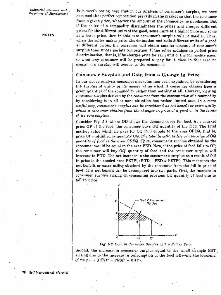
Industrial Economy and Principles of Management ■ It is worth noting here that in our analysis of consumer’s surplus, we have
assumed that perfect competition prevails in the market so that the consumer faces a given price, whatever the amount of the commodity he purchases. But if the seller of a commodity discriminates the prices and charges different prices for the different units of the good, some units at a higher price and some at a lower price, then in this case consumer’s surplus will be smaller- Thus, when the seller makes price discrimination and sells different units of a good at different prices, the consumer will obtain smaller amount of consumer’s surplus than under perfect competition. If the seller indulges in perfect price discrimination, that is, if he charges price for each unit of the commodity equal to what any consumer will be prepared to pay for it, then in that case no consumer’s surplus will accrue to the consumer.
NOTES
Cotisumer Surplut^ and Gain from a Change in PriceIn our above analysis consumer’s surplus has been explained by considering the surplus of utility or its money value which a consumer obtains from a given quantity of the commodity rather than nothing at all. However, viewing consumer surplus derived by the consumer from the consumption of a commodity by considering it in all or none situation has rather limited uses. In a more useful way, consumer’s surplus can be considered as net benefit or extra utility which a consumer obtains from the changes in price of a good or in the levels of its consumption.Consider Fig. 5.3 where DD shows the demand curve for food. At a market price OP of the food, the consumer buys OQ quantity of the food. The total market value which he pays for OQ food equals to the area OPEQ, that is, price OP multiplied by quantity OQ. The total benefit, utility or use-uatue ofOQ ' quantity of food is the area ODEQ. Thus, consumer’s surplus obtained by the consumer would be equal tb the area FED. Now, if the price of food falls to OP, the consumer will buy OQ' quantity of food and the consumer surplus will increase to P'TD. The net increase in the consumer’s surplus as a result of fall in price i.s the shaded area PETP’, (P’TD - PED » PETP’). This measures the net benefit or extra utility obtained by the consumer from the fall in price of food. This net benefit can be decomposed into two parts. First, the increase in consumer surplus arising on consuming previous OQ quantity, of food due to fall in price.
— Gain in Consumer Surplus
D
P
sTP'
D'
- Xo Q O'
Tig. 5.3. Gain in Consumer Surplus with a Fall m PriceSecond, the increase in consumer curp'.us equal to the small triangle EST arising duo to the increase in eohsumptiwii of the food folSuwing the lowering of ita pr -u (PETP' = PESP’ + EST';.
78 Self-Instructional Material
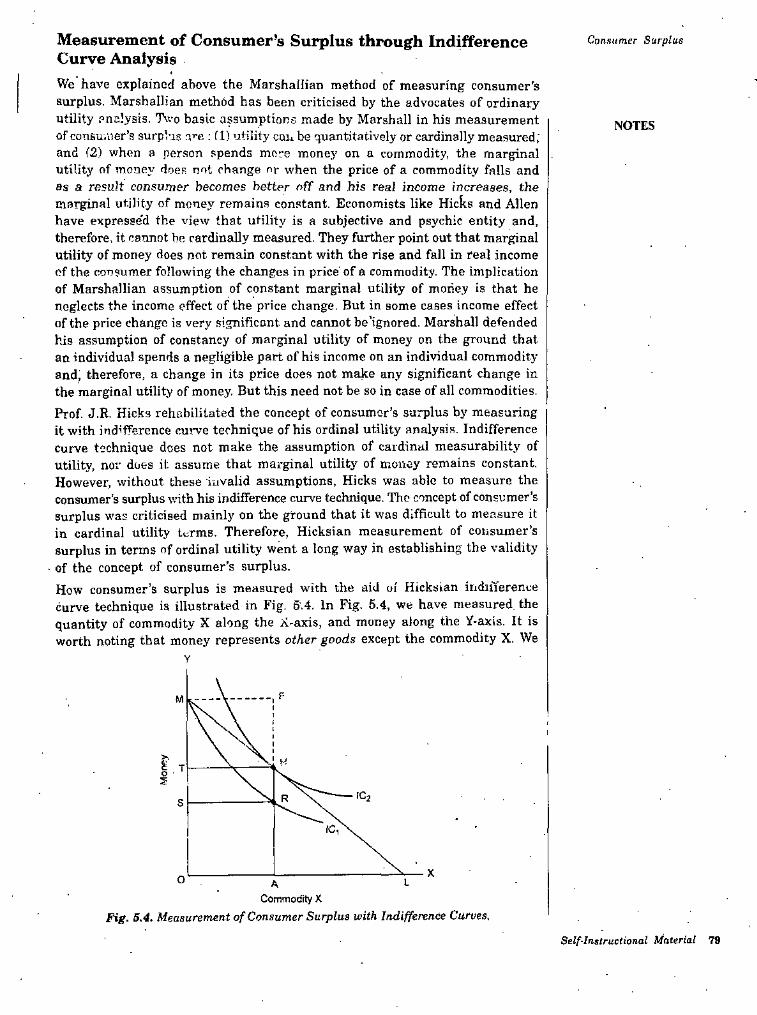
Measurement of Consumer’s Surplus through Indifference Curve Analysis
Consumer Surplus
We have explained above the Marshallian method of measuring consumer's surplus. Marshallian method has been criticised by the advocates of ordinary utility enalysis. Two basic assumptions made by Marshall in his measurement of consuviier’s surplus ^.re : fl) utility cau be quantitatively or cardinally measured; and (2) when a person spends mere money on a commodity, the marginal utility of money does, not change or when the price of a commodity falls and as a result consumer becomes better off and his real income increases, the marginal utility of money remains constant. Economists like Hicks and Allen have expresse'd the view that utility is a subjective and psychic entity and, therefore, it cannot be cardinaDy measured. They further point out that marginal utility of money does not remain constant with the rise and fall in real income of the consumer following the changes in price' of a commodity. The implication of Marshallian assumption of constant marginal utility of money is that he neglects the income effect of the price change. But in some cases income effect of the price change is very significant and cannot be’ignored. Marshall defended his assumption of constancy of marginal utility of money on the ground that an individual spends a negligible part of his income on an individual commodity and, therefore, a change in its price does not make any significant change in the marginal utility of money. But this need not be so in case of all commodities.Prof. J.R- Hicks rehabilitated the concept of consumer’s surplus by measuring it with indifference curve technique of his ordinal utility analysis. Indifference curve technique does not make the assumption of cardinal measurability of utility, nor does it assume that marginal utility of money remains constant. However, without these invalid assumptions, Hicks was able to measure the consumer’s surplus with his indifference curve technique. The concept of consumer’s surplus was criticised mainly on the ground that it was difficult to measure it in cardinal utility ti^rms. Therefore, Hicksian measurement of consumer’s surplus in terms of ordinal utility went a long way in establishing the validity
• of the concept of consumer’s surplus.
NOTES
How consumer’s surplus is measured with the aid of Hicksian indifference technique is illustrated in Fig. 5.4. In Fig. 5.4, we have measured thecurve
quantity of commodity X along the X-axis, and money along the Y-axis. It is worth noting that money represents other goods except the commodity X. We
Y
FM
HI.TIC2RS
1C
O LACommoefity X
Fig. 5.4. Measurement of Consumer Surplus with Indifference Curves.
Self-Instructional Material 79
Industriat Economy and EnncipUh of Manoficment have also shown some indifference curves between the given commodity X and
money for the consumer, the scale of his preference being given. Note that the . assumption of constant marginal utility of money requires that indifference curves are vertically parallel to each other. We know that consumer’s scale of preferences depends on his tastes and is quite independent of his income and market prices of the good. This will help us in understanding the concept of consumer's surplus with the aid of indifference curves.Suppose, a consumer has OM amount of money which he can spend on the commodity X and the remaining amount on other goods. The indifference curve IC, touches the point M indicating thereby that all combinations of money and commodity X represented on IC, give the same satisfaction to the consumer as OM aiuount of money. For example, take combination R on an indifference cu'.vc It follows that OA amount of coniinouity X and OSamount of money will give the same satisfaction to the consumer as OM amount of money because both M and R combinations lie on the same indifference curve ICj. In other words, it means that the consumer is willing to pay MS amount of money for OA amount of the commodity X. It is thus clear that, given the scale of preferences of the consumer, he derives the same satisfaction from OA amount of the commodity X as from MS amount of money. In other words, he is prepared to give up MS (or FR) for OA amount of commodity X.
NOTES
Now, suppose that the price of commodity X in the market is such that we getOM
i. We know from our analysis ofthe budget line ML (price of X is equal to consumer’s equilibrium that consumer would be in equilibrium where the given budget line is tangent to an indifference curve. It wilt be seen from Fig. 5.4 that the budget line ML is tangent to the indifference curve ICg at point H, where the consumer is having OA amount of commodity X and OT amount of money. Thus, given the market price of the commodity X, the consumer has actually spent MT amount of money for acquiring OA amount of commodity X. But, as mentioned above, he was prepared to forgo MS (or FR) amount of money for having OA amount ofX. Therefore, the consumer pays TS or HR less amount of money than he is prepared to pay for OA amount of the commodity X rather than go without it. Thus, TS or HR is the amount of consumer’s surplus which the consumer derives from purchasing OA amount of the commodity. In this way, Hicks explained consumer’s surplus with his indifference curves technique without assuming cardinal measurability of utility and without assuming constancy of the marginal utility of money. Since Marshall made these dubious assumptions for measuring consumer surplus, his method of measurement is regarded as invalid and Hicksian method of measurement with the technique of indifference curves is regarded as superior to the Marshallian method.
Critical Evaluation of the Concept of Consumer’s Surplus
The concept of consumer’s surplus has been severely criticised ever since Marshall propounded and developed it in his Principles of Economics. Critics have described it as quite imaginary’, unreal and useless. Most of the criticism of the concept has been levelled against the Marshallian method of measuring it as,an area under the demand curve. However, some critics have challenged the validity of the concept itself. Marshallian concept of consumer’s surplus has also been criticised on the ground of its being based upon unrealistic and questionable assumptions. We shall explain below the various criticisms levelled
I against this concept and will critically appraise them.
80 Self-Instructional Material
Consumer Surplus1. It has bfien pointed out by several economists that the concept of consumer's surplus is guile hypofhetical. imaginary and illusory. They say that a consumer cannot afford to pay for a commodity more than his income. The maximum amount which a person can pay for a commodity or for a number of commodities is limited by the amount of his money income. And, as is well-known, a consumer has a number of wants on which he has to spend his money. Total sum of money actually spent by him on the goods cannot be greater than his total money income. Thus what a person can be prepared to pay for a number of goods he purchases cannot be greater than the amount of his money income. Viewed in this light, there can bo no question of consumer getting any consumer’s surplus for his total purchases of the goods.But, in our view, the above criticism misses the real point involved in the concept of consumer’s surplus. The essence of the concept of consumer's surplus is that consumer gets excess psychic satisfaction from his purchases of the goods. It is true that with his limited money income, consumer cannot pay more for his total purchases than that he actually pays. But nothing prevents him from feeling and thinking that he derives more satisfaction from the goods than the price he pays for them and if be bad the means he would have been prepared to pay much more for the goods than he actually pays for them.
2. Another criticism against consumer’s surplus is that it is based upon the invalid assumption that different units of the goods give different amount of satisfaction to the consumer. We have explained above how Marshall calculated consumer’s surplus derived by the consumer from a good. Consumer purchases the amount of a good at which marginal utility is equal to its price. It is assumed that marginal utility of a good diminishes as the consumer has more units of it. This means that while at the margin of the purchase, marginal utility of the good is equal to its price, for the previous intramarginal units, marginal utility is highei' than the price and, on these intramarginal
■ units, consumer obtains consumer’s surplus. Now, the critics point out that when a consumer takes more units of a commodity it is not only the utility of the marginal unit that declines but also all previous units of the commodity he has taken. Thus, as all units of a commodity are assumed alike, all would have the same utility. And when, at the margin, price is equal to the marginal utility of the last unit purchased, the price will also be equal to the utility of the previous units and consumer would, therefore, not get any consumer’s surplus.But this criticism i.s ako not acceptable, because even though all units of a commodity may be alike, they do not give same satisfaction to the consumer; as consumer takes the first unit, he derives more satisfaction from it and when he takes up the second unit, it does not give him as much satisfaction as the first one, because while taking the second unit, a part of bis want has already been satisfied. Similarly, when he takes the third unit, it will not give him as much satisfaction as the previous two units, because now a part of his want has been satisfied. Similarly, when he takes the third unit, it will not give him as much satisfaction as the previous iwo units. If we accept the above criticism, we then deny the law of diminishing
NOTES
Self-Instructional Material 81
Industrial Economy and Principles of Management marpnal utility. But diminishing marginal utility from a good describes
the fundamental human tendency and has also been confirmed by observation of actual consumer’s behaviour. The concept of consumer’s surplus is derived from tho law of diminishing marginal utility. If law of diminishing marginal utility is valid, the validity of the Marshallian concept of consumer's surplus cannot be challonged.
3. The concept of consumer’s surplus has also been criticised on the ground that it ignorns the interdependence between the goods, that is, the relations of substitute and complementary goods. Thus, it.is pointed out that if only tea were available and no other substitute drinks such as milk, coffee, etc., were there, then the consumer would have been prepared to pay much more price for tea than that in the presence of substitute drinks. Thus, the magnitude of consumec’.s surplus derived from a commodity depends upon the availability of substitutes. This is because if only tea were available, consumer will have no choice and would be afraid that if he does not get tea, he cannot satisfy his given want from any other commodity. Therefore, he will be willing to pay more for a cup of tea rather than go without it. But if substitutes of tea are available, he would not be prepared to pay as much price since he will think that if he is deprived of tea, he will take other substitute drinks like milk and coffee. Thus, it is said that consumer’s surplus is not a definite, precise and unambip.ious concept; it depends upon the availability of substitutes. The degree of substitutability between different goods is different for different consumers, and this makes the concept of consumer’s surplus a little vague and ambiguous. Marshall was aware of this difficulty and, to overcome this, he suggested that, for the purpose of measuring consumer’s surplus, substitute products like tea and coffee be clubbed together and considered as one single commodity.
4. Prof Nicholson described the concept of consumer’s surplus as hji)othetjcal and imaginary. He writes, “of what avail is it to say that the utility of an income of (say) £ 100 a year is worth (say) £ 1000 a yoar". According to Prof. Nicholson and other critics, it is difficult to say how much price a consumer would be willing tr pay for a good rather than go without it.This is because consumer does' not face this question in the market when he buys goods; he has to pay and accept the price that prevails in the market. It is very difficult for him to say how much he would be prepared to pay rather than go without it. However, in our view, this criticism only indicates that it is difficult to measure consumer’s surplus precisely. That a consumer gets extra psychic satisfaction from a good than the price he pays for it’s undeniable.Moreover, as J.R. Hicks has pointed out “the best way of looking at consumer's surplus is to regard it as a means of expressing it in terms of money income gein which U; the ansumer .'»« aresult of a fall in price." the p-icc'of n cominodity falls, themoney income of the consumer being given, the piico line will switch to the right and the consumer will be in equilibriurr . at a higher indifference curve and as a result his satisfaction will increase. Thus, consumer derives more satisfaction at the lower price than that at the higher original price of the good. This implies that fall in the price of a commodity, and, therefore, the availability of the commodity
NOTES
62 Self-hstruciional Material
Consumer Surplusat a cheaper price adds to the satisfaction of the consuniPT' and this is in fact the change in consumer’s surplus brought about by change in the price of the good. Prof. J.R, Hicks has further extended the concept of consumer’s surplus considering it from the viewpoint of gain which a consumer gets from a fall in price of a good. Moreover, the concept of consumer’s surplus is useful and meaningful and not unreal because it indicates that he gets certain extra s..^tisfaction and advantages from the use of amenities available in civilised towns and cities.
5. The concept of consumer's surplus has also been criticised on the ground that it is based upon questionable assumptions of cardinal measurability of utility and constancy of the marginal utility of money. Critics point out that utility is a psychic entity and cannot be measured in quantitative cardinal terms. In view of this, they point but that consumer's surplus cannot be measured by the area under the demand curve, as Marshall did it. This is because Marshallian demand curve is based on the marginal utility curve in drawing which it is assumed that utility is cardinally measurable.Further, it has been explained in earlier chapters, by assuming constant marginal utility of money, Marshall ignored income effect of the price change. Of course, income effect of the price change in case of most of the commodities is negligible and can be validly ignored. But in case of some important commodities such as foodgrains, income effect of the price change is quite significant and cannot be validly ignored. Therefore, the Marshallian method of measurement of consumer surplus as area under the demand curve, ignoring the income effect, is not perfectly correct. However, this does not invalidate the concept of consumer’s surplus. As has been explained above, J.R. Hicks has been able to provide a money measure of consumer’s surplus with his indifference curve technique of ordinal utility analysis which does not assume cardinal measurement of utility and constant marginal utility of money. Hicks has not only rehabilitated the concept of consumer’s surplus but also extended and developed it further.
' Despite some of the shortcomings of the concept of consumer surplus, some of which are based on wrong interpretation of the concept of consumer surplus, it is of great significance not only in economic theory but also in the formulation of economic policies by the Government. The concept of consumer’s surplus has a great practical importance in the formulation of economic policies by the Government. We explain below some important uses and applications of consumer surplus.
NOTES
USES AND APPLICATIONS OF CONSUMER SURPLUSThe concept of consumer surplus has several applications both in economic theory and economic policy. This concept has been used to resolve water- diamond paradox of value theory, to explain the effects of teixes and subsidies on people’s welfare, to make cost-benefit analysis of public projects, to show gains from trade etc. We will explain below some of the applications of the concept of consumer surplus.
Self-Instructional Material 83
Induntrial Economy and Principlef of Management Explaining Water>Dianiond Paradox
One of the most famous puzzles in economic theory is why diamonds arc more expensive than water. Water is essential for life; it is so useful that without its consumption one cannot live or sun-ive. On the other hand, diamonds, though attractive and beautiful, satisfy less important human needs than water. Then, how it can be that in the market less useful commodity like diamonds arc so expensive and a highly useful commodity ns water is very cheap. Some thinkers in the past therefore complained that something was wrong with the market system which determines high price of commodities such os diamond, gold etc. which are least useful and low price of a commodity such as water which is necessary and highly useful. Therefore, this came to be known as water-diamond paradox. However, for modem economists there is no paradox about it as they arc able to explain the large price dilTerentiol of water and diamond. The notion of marginal utility or marginal benefit of a commodity and the concepts of consumer surplus based on it, can bo used to resolve the water-diamond paradox. The marginal benefit or marginal valuation per litre of’water for the consumer is very low as the actual supply of w’ater per period is very large.On the other hand, the marginal utility or marginal benefit of diamonds is verj' high because the amount of diamond actually available is very small. If, in fact, only few litres of water were available, marginal valuation of water would have been much greater than that of diamonds. Note that marginal i»o/uaf»o« of a commodity reflects how much amount of money consumer is prepared to pay for o commodity. This indicates marginal utility or use-value of the commodity for the consumer. It is worth noting that downward-sloping demand curve for a commodity can be interpreted as showing the marginal valuation or marginal utility in terms of money to the consumer of various units of a commodity. If the quantity actually available of a commodity in the market is very large, its marginal valuation or marginal utility will be very small, though its total use- value or total benefit may be very large. On the other hand, as the actually available quantity of a commodity such os diamonds, gold etc. is very small, its marginal valuation or marginal utility is very high, though its total valuc-in- use or total utilitj’ is small.Market price of a commodity is determined not by its total use-value but by its marginal valuation or marginal utility which in turn depends on the actually available quantity. The total use-value or total utility which a consumer gets from a quantity of a commodity equals the amount actually paid and the consumer surplus he obtains from it. In case of water market price as determined by its marginal utility is low but consumer surplus from it is very large. On the other hand, in case of diamond due to their greater scarcity, marginal utility and hence its price is large but consumer surplus from it is very small. Thus, the concept of consumer’s surplus shows that price should not Ire confused with total use-value of a commodity and this helps us to resolve the water- diamond paradox.This is illustrated in Fig. 6.5 where consumer’s demand cur/c depicts the marginal valuation curve for diomends. On the X-axis quantity of diamonds in grams per time period and along the Y-axis marginal utility or valuation and price of diamonds are measured. Since the total usc-value (».c., total utility) of diamond is small, the demand curve is at a low level. Suppose the quantity of diamond actually available is Qj and, as will be seen from the figure, price of diamond determined by demand and supply is which is quite high, whereas
NOTES
84 Self-tnnruetional Material
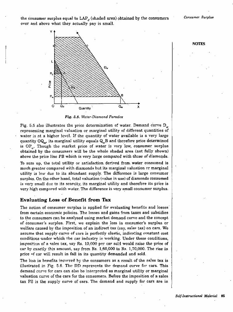
Consumer Surplusthe consumer surplus equal to LAP^ (shaded area) obtained by the consumers over and above what they actually pay is small.
Y\
NOTES
L
Dw
Po
8•c0.
0 Qa Qw XQjantity
Fig. S.5. Water-Diamond Paradox
Fig. 5.5 also illustrates the price determination of water. Demand curve representing marginal valuation or marginal utility of different quantities of water is at a higher level. If the quantity of water available is a very large quantity its marginal utility equals Q^B and therefore price determined is OP^., Though the market price of water is very low, consumer surplus obtained by the consumers will be the whole shaded area (not fully shown) above the price line PB which is very large compared with those of diamonds, lb sum up, the total utility or satisfaction, derived, from, water consumed is much greater compared with diamonds but its marginal valuation or marginal utility is low due to its abundant supply. The difference is large consumer surplus. On the other hand, total valuation (value in use) of diamonds consumed is very small due to its scarcity, its marginal utility and therefore its price is very high compared with water. The difference is very small consumer surplus.
Evaluating Loss of BeneHt from TaxThe notion of consumer surplus is applied for evaluating benefits and losses from certain economic policies. The losses and gains from taxes and subsidies to the consumers can be analysed using market demand curve and the concept of consumer’s surplus. First, we explain the loss in consumer’s surplus or welfare caused by the imposition of an indirect tax (say, sales tax) on cars. We assume that supply curve of cars is perfectly elastic, indicating constant cost conditions under which the car industry is working. Under these conditions, imposition of a sales tax, say Rs. 10,000 per car sold would raise the price of car by exactly this amount, say from Rs. 1,60,000 to Rs. 1,70,000. The rise in price nf car will result in fall in its quantity demanded and sold.The loss in benefits incurred by the consumers as a result of the sales tax is illustrated in Fig. 5.6. The DD represents the demand curve for cars. This demand curve for cars can also be interpreted as marginal utility or marginal valuation curve of the cars for the consumers. Before the imposition of a sales tax PS is the supply curve of cars. The demand and supply for cars are in
Self-Instructional Material 85
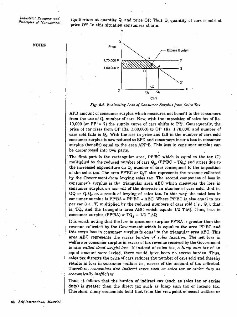
Industrial Economy and Principles of Management equilibrium at quantity Q, and price OP. Thus Q, quantity of cars is sold at
price OP. In this situation consumers obtain.Y
0NOTES Price
Excess Burden
1,70,000 P > '///'//.1,60,000 P
C
aQX0 QiQz
Cars
Fig. S.6. Evaluating Loss of Consumer Surplus from Sales Thx
APD amount of consumer surplus which measures net benefit to the consumers from the use of Q, number of cars. Now, with the imposition of sales tax of Rs. 10,000 (or PP's 7) the supply curve of cars shifts to P’S’. Consequently, the price of car rises from OP (Rs. 1,60,000) to OP' (Rs. 1,70,000) and number of cars sold falls to Qj. With the rise in price and fall in the number of cars sold consumer surplus is now reduced to BPD and consumers incur a loss in consumer surplus (benefit) equal to the area APP B. This loss in consumer surplus can be decomposed into two parts.The first part is the rectangular area, PPBC which is equal to the tax (T) multiplied by the reduced number of cars Qj. {PP'BC = TQj) and arises due to the increa.sed expenditure on Qg number of cars consequent to the imposition of the sales tax. The area PP’BC or QgT also represents the revenue collected by the Govemment-from levying sales tax. The second component of loss in consumer’s surplus is the triangular area ABC which measures the loss in consumer surplus on accc'int of the decrease in number of cars sold, that is, OQ or Q]Q2 as a result of levying of sales tax. In this way, the total loss in consumer surplus is PP'BA = PP'BC + ABC. Where PP’BC is also equal to tax per car {i.e., T) multiplied by the reduced numbers of cars sold (t.e., Q,), that . is, TQg and the triangular area ABC which equals 1/2 T.AQ! Thus, loss in consumer surplus (PP'BA) = TQj 1/2 T.aQ.It is worth noting that the loss in consumer surplus PP'BA is greater than the revenue collected by the Government which is equal to the area PP'BC and this extra loss in consumer surplus is equal to the triangular area ABC. This area ABC represents the excess burden of sales taxation. The net loss in welfare or consumer surplus in excess of tax revenue received by the Government is also called dead weight loss. If instead of sales tax, a lump sum tax of an equal amount were levied, there would have been no excess burden. Thus, sales tax distorts the price of cars reduces the number of cars sold and thereby results in loss in consumer v/elfare in , excess of the amount of tax collected. Therefore, economists dub indirect taxes such as sales tax or excise duty as economically inefficient.
Thus, it follows that the burden of indirect tax (such as sales tax or excise duty) is greater than the direct tax such as lump sum tax or income tax. Therefore, many economists hold that from the viewpoint of social welfare or
88 Self-Instructional Material
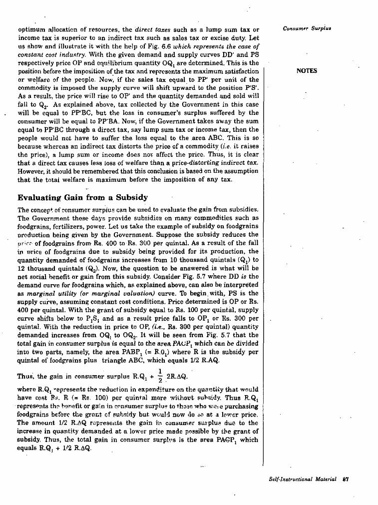
Conaumfr SurpluaOptimum ajlocation of resources, the direct taxes such as a lump sum tax or income tax is superior to an indirect tax such as sales tax or excise duty. Let us show and illustrate it with the help of Fig. 6.6 which represents the case of constant cost industry. With the given demand and supply curves DD’ and PS respectively price OP and equilibrium quantity OQj are determined. This is the position before the Imposition of the tax and represents the maximum satisfaction or welfare of the people. Now, if the sales tax equal to PP' per unit of the commodity is imposed the supply curve will shift upward to the position P'S'. As a result, the price will rise to OP' and the quantity demanded and sold will fall to Qj. As explained above, tax collected by the Government in this case will be equal to PP'BC, but the loss in consumer’s surplus suffered by the consumer will be equal to PP'BA. Now, if the Government takes away the sum equal to PP'BC through a direct tax, say lump sum tax or income tax, then the people would not have to suffer the loss equal to the area ABC. 'This is so because whereas an indirect tax distorts the price of a commodity (i.e. it raises the price), a lump sum or income does nor affect the price. Thus, it is clear that a direct tax causes less loss of welfare than a price-distorting indirect tax. However, it should be remembered that this conclusion is based on the assumption that the total welfare is maximum before the imposition of any tax.
NOTES
Evaluating Gain from a Subsidy'The concept of consumer surpius can be used to evaluate the gain from subsidies. The Government these days provide subsidies on many commodities such as foodgrains, fertilizers, power. Let us take the example of subsidy on foodgrains oroduction being given by the Government. Suppose the subsidy reduces the rjr irr of foodgrains from Rs. 400 to Rs. 300 per quintal. As a result of the fall in nrice of foodgrains due to subsidy being provided for its production, the quantity demanded of foodgrains increases from 10 thousand quintals (Qj) to 12 thousand quintals (Qj)- Now, the question to be answered is what will be net social benefit or gain from this subsidy. Consider Fig. 5.7 where DD is the demand curve for foodgrains which, as explained above, can also be interpreted as marginal utility (or marginal valuation) curve, lb begin, with, PS is the supply cuiwe, assuming constant cost conditions. Price determined is OP or Rs. 400 per quintal. With the grant of subsidy equal to Rs. 100 per quintal, supply curve shifts below to PjS, and as a result price falls to OPj or Rs. 300 per quintal. With the reduction in price to OP, (i.e., Rs. 300 per quintal) quantity demanded increases from OQ, to OQj. It will be seen from Fig. 5.7 that the total gain in consumer surplus is equal to the areaPAcFi which can be divided into two parts, namely, the area PABPj (= R.Oj) where R is the subsidy per quintal of foodgrains plus triangle ABC, which equals 1)2 R.AQ.
Thus, the gain in consumer surplus R.Q^ + 2R.AQ.
where R.Q, -epresents the reduction in expenditure on the quantity that would have cost Rs. R (= Rs. 100) per quintal more without subsidy. Thus R.Qj represents the benefit or gam in consumer surplus to those who weie purchasing foodgrains before the grout of subsidy but would now do 6!> at a lower price. The amount 1/2 R.AQ rapresents the gain in consumer suiplus due to the increase in quantity demanded at a lower price made possible by the grant of subsidy, Thus, the total gain in consumer surplus is the area PAGPj which equals R.Qj + 1/2 R.AQ.
Seif-Instru-ctional Material 87
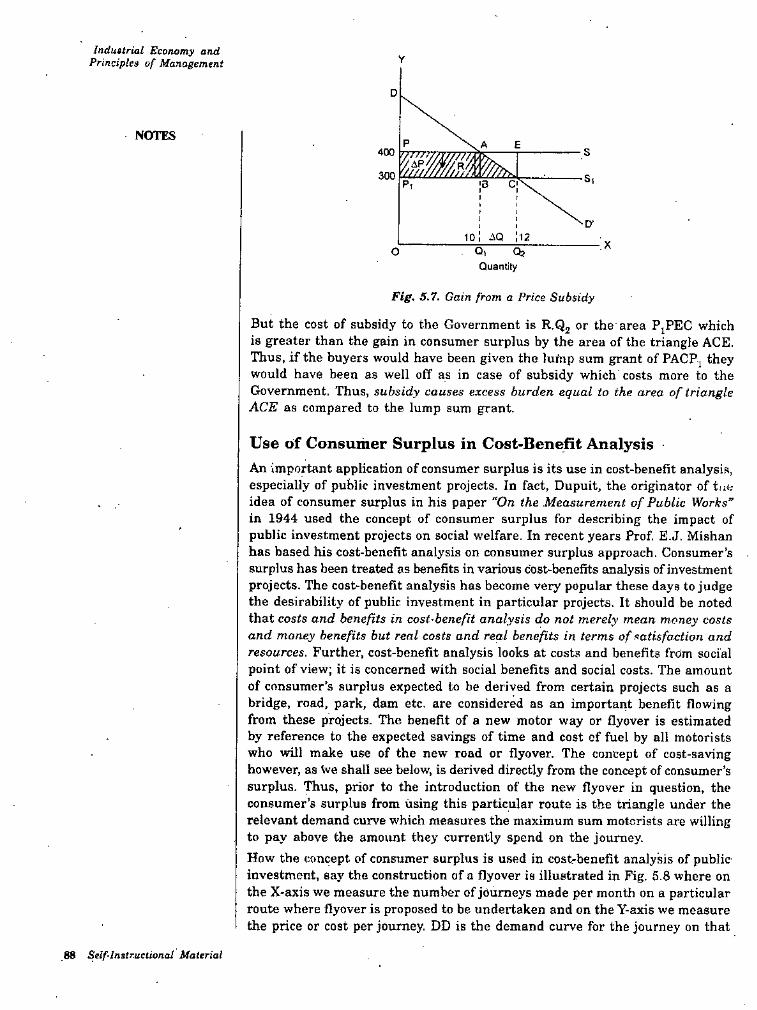
Industrial Economy and Principles of Management
D
NOTES400
3003 CPi
10 1 ilQX
QtO 02Quantity
Fig. 5.7. Cain from a Price Subsidy
But the cost of subsidy to the Government is R.Qj or the area PjPEC which is greater than the gain in consumer surplus by the area of the triangle ACE. Thus, if the buyers would have been given the lump sum grant of PACPj they would have been as well off as in case of subsidy which costs more to the Government. Thus, subsidy causes excess burden equal to the area of triangle ACE as compared to the lump sum grant.
Use of Consumer Surplus in Cost>Benefit AnalysisAn important application of consumer surplus is its use in cost-benefit analysis especially of public investment projects. In fact, Dupuit, the originator of t idea of consumer surplus in his paper “On the Measurement of Public Works” in 1944 used the concept of consumer surplus for describing the impact of public investment projects on social welfare. In recent years Prof. E.J. Mishan has based his cost-benefit analysis on consumer surplus approach. Consumer’s surplus has been treated as benefits in various cost-benefits analysis of investment projects. The cost-benefit analysis has become very popular these days to judge the desirability of public investment in particular projects. It should be noted that costs and benefits in cost-benefit analysis do not merely mean money costs and money benefits but real costs and real benefits in terms of satisfaction and resources. Further, cost-benefit analysis looks at costs and benefits from social point of view; it is concerned with social benefits and social costs. The amount of consumer’s surplus expected to be derived from certain projects such as a bridge, road, park, dam etc. are considered as an important benefit flowing from these projects. The benefit of a new motor way or flyover is estimated by reference to the expected savings of time and cost of fuel by all motorists who will make use of the new road or flyover. The concept of cost-saving however, as We shall see below, is derived directly from the concept of consumer’s surplus. Thus, prior to the introduction of the new flyover in question, the consumer's surplus from using this particular route is the triangle under the relevant demand curve which measures the maximum sum motorists are willing to pay above the amoimt they currently spend on the journey.How the concept of consumer surplus is used in cost-benefit analysis of public investment, say the construction of a flyover is illustrated in Fig. 5.8 where on the X-axis we measure the number of journeys made per month on a particular route where flyover is proposed to be undertaken and on the Y-axis we measure the price or cost per journey. DD is the demand curve for the journey on that
J
.88 Self-Inatruetional Material
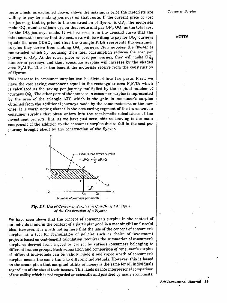
Consumer Surplusroute which, as explained above, shows the maximum price the motorists are willing to pay for making journeys on that route. If the current price or cost per journey, that is, prior to the construction of flyover is OPj, the motorists make OQj number of journeys on that route and pay OPj. OQj as the total cost for the OQ, journeys made. It will be seen from the demand curve that the total amount of money that the motorists will be willing to pay for OQ, journeys equals the area ODAQ, and thus the triangle P,DA represents the consumer surplus they derive from making OQ, journeys. Now suppose the flyover is constructed which by reducing their fuel consumption reduces the cost per journey to OP2- At the lower price or cost per journey, they will make OQj number of journeys and their consumer surplus w'ill increase by the shaded area PjACPj. This is the benefit the motorists receive from the construction of flyover.•This increase in consumer surplus can be divided into two parts. First, we have the cost saving component equal to the rectangular area Pj'PjTA which is calculated as the saving per journey multiplied by the original number of journeys OQ,. The other part of the increase in consumer surplus is represented by the area of the triangle ATC which is the gain in consumer’s surplus obtained from the additional journeys made by the same motorists or the new ones. It is, worth noting that it is the cost-saving segment of the increment in consumer surplus that often enters into the cost-benefit calculations of the investment projects. But, as we have just seen, this cost-saving is the main component of the addition to the consumer surplus due to fall in the cost per journey brought about by the construction of the flyover.
NOTES
Y
D
Gain in Consumer Surplus = -\P.Qi y i.\P:\Q
APi
PaT
DAQ
0 Qi 02Number of journeys per month
Fig. 5.8. Use of Consumer Surplus in Cost-Benefit Analysis of the Construction of a Flyover
We have seen above that the concept of consumer’s surplus in the context of an individual and in the context of a particular good is a meaningful and useful idea. However, it is worth noting here that the use of the concept of consumer’s surplus as a tool for formulation of policies such as choice of investment projects based on cost-benefit calculation, requires the summation of consumer’s surpluses derived from a good or project by various consumers belonging to different income groups. Such summation and comparison of consumer’s surplus of different individuals can be validly made if one rupee worth of consumer’s surplus means the same thing to different individuals. However, this is based on the assumption that marginal utility of money is the same for all individuals regardless of the size of their income. This lands us into interpersonal comparison of the utility which is not regarded as scientific and justified by many economists.
Self-Instructhnal Material 69
Indutlrial Economy and Principles of Management
STUDENT ACTIVITY
1. What is meant by consumer’s surplus ? How can consumer’s surplus be measured?
2. Explain graphically the concept of consumer’s surplus.
i-
80 Se^-Tnetruefienal Material
Consumer SurplusSUMMARY
• Consumer surplus measures extra utility or satisfaction -which a consumer obtains from Uie consumption of a certain amount of commodity over and above the utility of its market value.
• In a more useful way, consumer’s surplus can be considered as net beneht or extra utility which a consumer obtains from the changes in price of a goods or in the levels of its consumption.
• Costs and benefits in cost^benefit analysis do not merely mean money costs and money benefits but reel costs and real benefits in terms of satisfaction and resources.
NOTES
REVIEW EXERCISES1. -Define consumer's surplus and discuss the applications of the concept.
of consumer’s surplus.2. Explain the meaning and limitations of consumer’s surplus.
Stlf-lrtstruelional Material 9t
Industrial Economy and Principles of Management UNIT 6 ELASTICITY OF DEMAND
★ STRUCTURE ★NOTES
□ Price Elasticity of DemandQ Measurement of Price Elasticity□ Determinants of Price Elasticity of Demand□ Importance of the Price Elasticity of Demand□ Cross Elasticity of Demand□ Income Elasticity of Demand
Various Concepts of Demand ElasticityWhen the price of a good falls, its quantity demanded rises and when the price of its rises, its quantity demanded falls. This is generally known as law of demand. This law of demand indicates only the director of change in quantity demanded in response to a change in price. This does not tell us by how much or to what extent the quantity demanded of a good will change in response to a. change in its price. This information as to how much or to what extent the quantity demanded of a good will change as a result of a change in its price is provided by the concept of elasticity of demand.It is price elasticity of demand which is usually referred to as elasticity of demand. But, besides price elasticity of demand, there are various other concepts of demand elasticity. As we have seen in the-previous chapter, demand for a good is determined by its price, incomes of the people, prices of related goods, etc. Quantity demanded of a good will change as a result of change in any of these determinants of demand. The concept of elasticity of demand therefore refers to the degree of responsiveness of quantity demanded of a good to a change in its price, consumers’ income and prices of related goods. Accordingly, there are three concepts' of demand elasticity ; price elasticity, income elasticity, and cross elasticity, Price elasticity of demand relates to the degree of responsiveness of quantity demanded of a good to the change in consumers’ its price. Income elasticity of demand refers to the sensitiveness of quantity demanded to the change in income. Cross elasticity of demand means the degree of responsiveness of demand of a good to a change in the price of a related good, which may be either a substitute for it or a complementary with it.The concept of elasticity of demand forms the subject-matter of the present chapter. The concept of elasticity has "a very great importance in economic theory as well as for formulation of suitable economic policies.
PRICE ELASTICITY OF DEMANDAs mentioned above, price elasticity of demand indicates the degree of responsiveness of quantity demanded of a good to the change in its price, other factors such
92 Self-Instructional Material
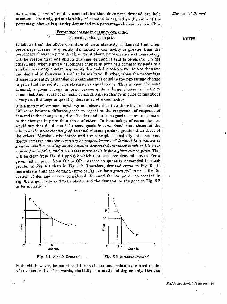
as income, prices of related commodities that determine demand are held constant. Precisely, price elasticity of demand is defined as the ratio of the percentage change is quantity demanded to a percentage change in price. Thus
Elasticity of Demand
Percentage change in quantity demandede
p Percentage change in price NOTESIt follows from the above definition of price elasticity of demand that when percentage change in quantity demanded a commodity is greater than the percentage change in price that brought it about, price elasticity of demand (c^) will be greater than one and in this case demand is said to be elastic. On the other hand, when a given percentage change in price of a commodity leads to a smaller percentage change in quantity demanded, elasticity will be less than one and demand in this case is said to be inelastic. Further, when the percentage change in quantity demanded of a commodity is equal to the percentage change in price that caused it, price elasticity is equal to one. Thus in case of elastic demand, a given change in price causes quite a large change in quantity demanded. And in case of inelastic demand, a given change in price brings about a very small change in quantity demanded of a commodity.It is a matter of common knowledge and observation that there is a considerable difference between different goods in regard to the magnitude of response of demand to the changes in price. The demand for some goods is more responsive to the changes in price than those of others. In terminology of economics, we would say that the demand for some goods is more elastic than those for the others or the price elasticity of demand of some goods is greater than those of the others. Marshall who introduced the concept of elasticity into economic theory remarks that the elasticity or responsiveness of demand in a market is great or small according as the amount demanded increases much or little for a given fall in price, and diminishes much or little for a given rise in price. This will be clear from Fig. 6.1 and 6.2 which represent two demand curves. For a given fall in price, from OP to OP, increase in quantity demanded is much greater in Fig. 6.1 than in Fig. 6.2. Therefore, demand curve in Fig. 6.1 is more elastic than the demand curve of Fig. 6.2 for a given fall in price for the portion of demand curves considered. Demand for the good represented in Fig. 6.1 is generally said to be elastic and the demand for the good in Fig. 6.2 to be inelastic. •
DD
pp
P’ p'DS s-c0. a
D
XWo M O N N-Quantity Quantity
Fig. E.2. Inelastic DemandFig. 6.1. Elastic Demand
It should, however, be noted that terms elastic and inelastic are used in the relative sense. In other words, elasticity is a matter of degree only. Demand
Self-Instructiorial Material 93
Industrial Economy and Principles of Management
for some goods is only more or less elastic than others. Thus, when we say that demand for a good is elastic, we mean only that the demand for it is relatively more clastic. Likewise, when we say that demand for a good is inelastic, we do not mean that its demand is absolutely inelastic but only that it is relatively less elastic. Tn economic theory elastic and inelastic demands have come to acquire precise meanings. Demand for a good is said to be elastic if the price elasticity of demand for it is greater than one. Similarly, the demand for a good is called inelastic if price elasticity of demand for it is less than one. Price elasticity of demand equal to one, or in other words, unit elasticity of demand therefore represents the dividing line between elastic and inelastic demand. It will now be clear that by inelastic demand wc do not mean perfectly inelastic put only that the elasticity of demand is less than unity; and by elastic demand we do not mean absolutely elastic but that tiie elasticity of demand is greater than one.Thus,Elastic demand Inelastic demand Unitary elastic demand
NOTES
1
= 1
Price Elasticity of Demand for Different Goods Varies a Good DealAs said above, goods show great variation in respect of elasticity of demand i.e., their responsiveness to changes in price. Some goods like common salt, wheat and rice are very unresponsive to the changes in their prices. The demand for salt remains practically the same for a small rise or fall in its price. Therefore, demand for common salt is said to be ‘inelastic’. Demand for goods like radios, refrigerators etc., is elastic, since changes in their prices bring about large changes in their quantity demanded. We shall explain later at length those factors which are responsible for the differences in elasticity of demand of various goods. It will suffice here to say that the main reason for differences in elasticity of demand is the Possibility of substitution i.e., the presence or absence of competing substitutes. The greater the ease with which substitutes can be found for a commodity or with which it can be substituted for other commodities, the greater will be the price elasticity of demand of that commodity.
Goods are demanded because they satisfy some particular wants and in general wants can be satisfied in a variety of alternative ways. For instance, the want for entertainment can be gratified by having television set, or by possessing a gramophone, or by going to cinemas or by visiting theatres. If the price of a television set falls, the quantity demanded of television sets will rise greatly since fall in the price of television will induce some people to buy televisions in place of having gramophones or visiting cinemas and theatres. Thus the demand for televisions is elastic, Likewise, if the price of‘Lux’ falls, its demand will greatly rise because it will be substituted for other varietie.? of soap such as Jai, Hamam, Godrej, Pears etc. On the contrary, the demand for a necessary good like salt is inelastic. The demand for salt is inelastic since it satisfies a basic human want and no substitutes for it are available. People would consume almost the same quantity of salt whether it becomes slightly cheaper or dearer than before.
94 Self-Ir\iructional Material
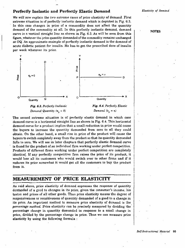
Elasticity of DemandPerfectly Inelastic and Perfectly Elastic DemandWe will now explain the two extreme cases of price elasticity of demand. First extreme situation is of perfectly inelastic demand which is depicted in Fig. 6.3. In this case changes in price of a commodity does not affect the quantity demand of the commodity at all. In this perfectly inelastic demand, demand curve is a vertical straight line as shown in Fig. 6.3. As will be seen from this figure, whatever the price quantity demanded of the commodity remains unchanged at OQ. An approximate example of perfectly inelastic demand is the demand of acute diabetic patient for insulin. He has to get the prescribed doze of insulin per week whatever its price.
NOTES
YY
D
8•w0.
8•c ep = o P D0.
XXo GQ QuantityQuantity
Fig. 6.3. Perfectly Inelastic Demand Quantity (e^ = 0)
The second extreme situation is of perfectly elastic demand in which case demand curve is a horizontal straight line as shown in Fig. 6.4. This horizontal demand curve for a product implies that a small reduction in price would cause the buyers to increase the quantity demanded from zero to all they could obtain. On the other hand, a small rise in price of the product will cause the buyers to switch completely away from the product so that its quantity demanded falls to zero, We will see in later chapters that perfectly elastic demand curve is found for the product of an individual firm working under perfect competition. Products of different firms working under perfect competition are completely identical. If any perfectly competitive firm raises the price of its product, it would lose all its customers who would switch over to other firms and if it reduces its price somewhat it would get all the customers to buy the product from it.
Fig. 6.4. Perfectly Elastic Demand (e^ = e)
MEASUREMENT OF PRICE ELASTICITYAs said above, price elasticity of demand expresses the response of quantity dcnl'anded of a good to changes in its price, given the consumer’s income, his tastes and prices of all other goods. Thus price elasticity means the degree of responsiveness or sensitiveness of quantity demanded of a good to a change in its price. An important method to measure price elasticity of demand is the percentage method. Price elasticity can be precisely measured by dividing the percentage change in quantity demanded in response to a small change in price, divided by the percentage change in price. Thus we can measure price elasticity by using the following formula :
Self-Instructional Material 95
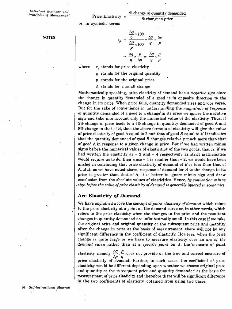
Industrial Economy and Principles of Management % change in quantity demanded
Price Elasticity =
or, in symbolic terms% change in price
AgxlOO
NOTES Ag Ap ^xlOO ^ Pp
P
q- pq dp
where stands for price elasticityq stands for the original quantity p stands for the original price A stands for a small change
Mathematically speaking, price elasticity of demand has a negative sign since the change in quantity demanded of a good is in opposite direction to the change in its price. When price falls, quantity demanded rises and vice versa. But for the sake of convenience in understanding the magnitude of fesponse of quantity demanded of a good to a change’in its price we ignore the negative sign and take into account only the numerical value of the elasticity- Thus, if 2% change in price leads to a 4% change in quantity demanded of good A and 8% change in that of B, then the above formula of elasticity will give the value of price elasticity of good A equal to 2-and that of good B equal to 47 It indicates that the quantity demanded of good B changes relatively much more than that of good A in response to a given change in price. But if we had written minus signs before the numerical values of elasticities of the two goods, that is, if we had written the elasticity as - 2 and - 4 respectively as strict mathematics would require us to do, then since — 4 is smaller thain - 2, we would have been misled in concluding that price elasticity of demand of B is less than that of A. But, as we have noted above, response of demand for B to the change in its price is greater than that of A, it is better to ignore minus sign and draw conclusion from the absolute values of elasticities. Hence, by convention minus
. sign before the value of price elasticity of demand is generally ignored in economics.
Arc Elasticity of DemandWe have explained above the concept of point elasticity of demand which refers to the price elasticity at a point on the demand curve or, in other words, which refers to the price elasticity when the changes in the price and the resultant changes in quantity demanded are infinitesimally small. In this case if we take the original price and original quantity or the subsequent price and quantity after the change in price as the basis of measurement, there will not be any significant difference in the coefficient of elasticity. However, when the price change is quite large or we have to measure elasticity over an arc of the demand curve rather than at a specific point on it, the 'measure of point
elasticity, namely
price elasticity of demand. Further, in such cases, the coefficient of price elasticity would be different depending upon whether we choose original price and quantity or the subsequent price and quantity demanded as the basis for measurement of price elasticity and vherefore there will be significant difference in the two coefficients of elasticity, obtained from using two bases.
Aq p. — does not provide us the true and correct measure ofAp q
96 Self-Instructional Material
Elasticity of DemandTherefore, when the change in price is quite large, say more than 10 percent, then accurate measure of price elasticity of demand can be obtained by taking the average of original price and subsequent price as well as average of the original quantity and subsequent quantity as the basis of measurement of percent^e changes in price and quantity. Thus, if price of a good falls from pj to pgand as a result its quantity demanded increases from q, to q^, the-average
A +P2
NOTES
and average of the two quantities (originalof the two prices is given by2
Thus, the formula for measuring arc
elasticity, that is, when change in price is quite large is given byand subsequent) is given by
e = ^A+A ' P1+P2p
22A? P1+P2 _ ^ Pi + Pi
= q.-t- qj ■ Ap ■ Ap ' q, -t- 92
Let us solve some numerical problems of price elasticity of demand'Cboth point and arc) by percentage method.Problem 1. Suppose the price of a commodity falls from Rs. 10 to Rs. 9 per unit and due to this quantity demanded of the commodity increases from 100 units to 120 units. Find out the price elasticity of demand.
■ Sol.Change in price (AP) = Rs. 10 - 9 = Re. 1 Original price (Pj) = Rs. 10
• Change in quantity (Aq) = 120 - 100 = 20 Original quantity = 100
Aq Pep Ap q
Substituting the values of Aq, Ap, p and q we have
e = = 21 100 . _
Problem 2. A consumer purchases 80 units of a commodity when its price is Re. 1 per unit and purchases 48 units when its price rises to Rs. 2 per unit. What is the price elasticity of demand for the commodity^Sol. It should be noted the change in price from Re. 1 to Rs. 2 in this case is very large (i.e., 100%). Therefore, to calculate the elasticity coefficient in this case arc elasticity formula should be used.
Change is price (Ap) = Rs. 2-1 = 1.
p
P1 + P2Average of the original and subsequential prices =A
1-^2 32 "2 •
Change in quantity demanded (Aq) = 80 - 48 = 32
= 1.5SS
Average of the original and subsequent quantities =
• 80■^48 1282
Self-Instructional Material 97
Industrial Economy and Principles of Management
= ?1+92 P,+ P22 2
32 1NOTES — -f64 1.5
32 1.5 1 15 3= — a- s 0.7564 1 2 10 4— XSC
Thus, the price arc elasticity of demand obtained is equal to 0,75,Problem 3. Suppose a seller of a textile cloth wants to lower the price of its cloth from 150 per metre to Rs. 142.5 per metre. If its present sales are 2000 metres per month and further it is estimated that its elasticity of demand for the product equals - 0.7. Show (a) Whether or not his total revenue will increase as a result of his price; and (b) Calculate the exact magnitude of its new total revenue.
^ PAp'q
p = Rs, 150 q = 2000 metres
4P = 150 - 142.5 = 7.5
Sol. (a) Price elasticity =
= 0.7%6q =?
•Substitu-ting the values ofp, q, lup and in the price elasticity formula we have
- -^x ■ 7,5 2000
1500.7
0.7x7.5x2000 = 70Hq150
Since price has fallen quantity demanded will increase by 70 metres. So the nev/ quantity demanded will be 2000 + 70 = 2070.ib) Total Revenue before reduction in price = 2000 x 150 = Rs. 3,00,000 Tbtal revenue after reduction 2070 X 142.5 = Rs. 2,94,975, • Thus with reduction in price his total revenue has decreased.
ss
Total Espenditure or Total Revenue MethodWe have explained above the percentage method of measurement of price elasticity of demand. There is also another method to measure price elasticity of demand. This is known as total expenditure method or total revenue method. The price elasticity of demand for a good and the total expenditure made on the good are greatly related to each other. From the changes in the total expenditure made on a good as a result of change.s in its price, we can know the price elasticity of demand for the good. But it should be remembered that with the total expenditure method we can know only whether elasticity is equal to one, greater than one or less than one. With this method we cannot find out the exact and precise coefficient of elasticityUnit elasticity (e^ = 1). When as a result of the change in price of a good the quantity demanded o/ the good increases so much that the total expenditure
98 Self-Instructional Material
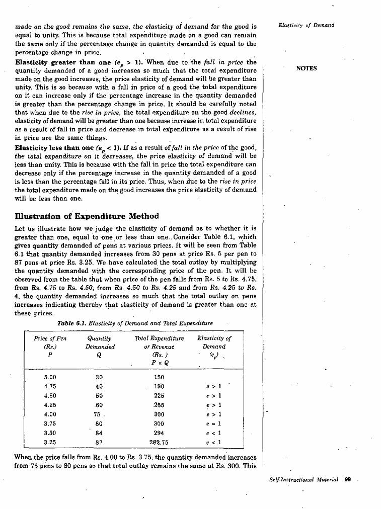
Elasticity of Demandmade on the good remains the same, the elasticity of demand for the good is equal to unity. This is because total expenditure made on a good can remain the same only if the percentage change in quantity demanded is equal to the percentage change in price.Elasticity greater than one (e^ > 1). When due to the fall in price the quantity demanded of a good increases so much that the total expenditure made on the good increases, the price elasticity of demand will be greater than unity. This is so because with a fall in price of a good the total expenditure on it can increase only if the percentage increase in the quantity demanded is greater than the percentage change in price. It should be carefully noted that when due to the rise in price, the total expenditure on the good declines, elasticity of demand will be greater than one because increase in total expenditure as a result of fall in price and decrease in total expenditure as a result of rise in price are the same things.Elasticity less than one (e^ < 1). If as a result of fall in the price of the good, the total expenditure on it decreases, the price elasticity of demand will be less than unity. This is because with the fall in price the total expenditure can decrease only if the percentage increase in the quantity demanded of a good is less than the percentage fall in its price. Thus, when due to the rise in price the total expenditure made on the good increases the price elasticity of demand will be less than one.
NOTES
Illustration of Expenditure MethodLet us illustrate how we judge the elasticity of demand as to whether it is greater than one, equal to-one or less than one.. Consider Table 6.1, which gives quantity demanded of pens at various prices. It will be seen from Table 6-1 that quantity demanded increases from 30 pens at price Rs. 5 per pen to 87 pens at price Rs. 3.25. We have calculated the total outlay by multiplying the quantity demanded with the corresponding price of the pen. It will be observed from the table that when price of the pen falls from Rs. 5 to Rs. 4.75, from Rs. 4.75 to Rs. 4.50, from Rs. 4.50 to Rs. 4.25 and from Rs. 4.25 to Rs. 4, the quantity demanded increases so much that the total outlay on pens increases indicating thereby that elasticity of demand is greater than one at these prices-
Table 6.1. Elasticity of Demand and Thtal Expenditure
QuantityDemanded
Total Expenditure or Revenue
(Rs.) PyQ
Elasticity of Demand
V -
Price of Pen (Rs.)
P Q
5.00 15030. 190 e > 1
<> > 1 e > 1 e > 1
4.75 402254,50 50
.2554.25 .604,00 30075 .3.75 30080 e = 13.50 84 294 c < 1
e < 13.25 87 282.75
When the price falls from Rs. 4.00 to Rs. 3.75, the quantity demanded increases from 75 pens to 80 pens so that total outlay remains the same at Rs. 300. This
Self-Instructional Material 99
Industrial Economy and Principles of Management shows that price elasticity of demand is unity When the price of the pen
further falls from Rs. 3.75 to Rs. 3.50 and then to Rs. 3.25 the total outlay spent on pens decrease.^, Thus, the elasticity of demand for pens at these prices is less than unity.Problem 4. Suppose price of a good falls from Rs. 10 to Rs. 8 per unit. As a result, its quantity demanded increases from 80 units to 100 units. What can we say about price elasticity of demand by total revenue method.Sol. At price Rs. 10, quantity demand is 100 units.Therefore, total revenue at price Rs. 10 = P x Q = 10 x 80 = Rs. 800 At the lower price Rs. 8, quantity, demand increases to 100 units.Therefore, total revenue at price Rs. 8 = PxQ = 8x 100 = Rs. 800 We thus find that with the change in price of the good, total revenue of the firm remains constant. Hence price elasticity of demand is equal to one. Problem 5. Suppose price of a commodity rises from Rs. 15 to Rs. 16 per unit. As a result, its quantity demanded falls from Rs. 100 units to 80 units. Find out the price, elasticity of demand by expenditure method.Sol. Expenditure on the commodity at price
Rs. 15 = P X Q = 15 X 100 = Rs. 1500 Expenditure on the commodity at price Rs. 16 = 16 x 80 = Rs. 1,280 Thus we find with the rise in price, expenditure on the commodity decreases. This means the price elasticity of demand is greater than one (e^ > 1). Problem 6. Suppose that price elasticity of demand for petrol is equal to unity and at Rs. 15 per litre an individual consumes (i.e., demands) 80 litres of petrol in a week. How much price'of petrol should be fixed so that he demands 60 litres of petrol?Sol. Since the given price elasticity of demand for petrol is equal to unity, the expenditure on the petrol by the individual will remain constant at different prices.Expenditure on petrol at price of
Rs. 15 per litre = P x Q = 15 x 80 = Rs. 1,200 Let the higher price of petrol be P', the expenditure on the petrol by the consumer so that he demands 60 litres of-petrol per week is then given by
P' X 60 = Rs. 1200 1200
NOTES
= Rs. 20P' = 60Thus we find that price of petrol be raised to Rs. 20 per litre so as to reduce individual demand for petrol to 60 litres per week.
Graphic Illustration of Expenditure MethodThis relationship between the price elasticity of demand and total outlay can also be graphically illustrated with the aid of the demand curve. This relationship between price elasticity of demand and total expenditure, made on good is illustrated with the aid of Fig. 6.5 where demand curve DD Ls given. In the Fig. 6.5 when the price is OP, the total expenditure made on the good is equal to OP X OQ i.e., area OPRQ and when the price falls to OP', the total expenditure is equal to OP'R'Q'. It will be seen from the Figure 6.5 that the area OP'HQ is common in both the rectangles OPRQ and OP'R'Q'. Now, by comparing the remaining areas PRHP and QHR'Q' we find that two are equal to each other.
100 Self-Instructional Material
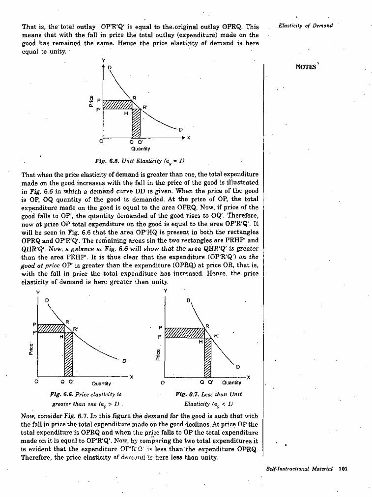
Elasticity of DemandThat is, the total outlay OP’R'Q' is equal to the.original outlay OPRQ. This means that with the fall in price the total outlay (expenditure) made on the good has remained the same. Hence the price elasticity of demand is here equal to unity. '
>NOTES
I Pa.
P' H
► Xo Q O'Quantity
Fig. 6.5. Unit Elasticity TCp = 1)
That when the price elasticity of demand is greater than one, the total expenditure made on the good increases with the fall in the price of the good is illustrated in Fig. 6.6 in which a demand curve DD is given. When the price of the good is OP, OQ quantity of the good is demanded. At the price of OP, the total expenditure made on the good is equal to the area OPRQ. Now, if price of the good falls to OP', the quantity demanded of the good rises to OQ'. Therefore, now at price OP total expenditure on the good is equal to the area OP'R'Q'. It will be seen in Fig. 6.6 that the area OP'HQ is present in both the rectangles OPRQ and OP'R'Q'. The remaining areas sin the two rectangles are PRHP' and QHR'Q'. Now, a galance at Fig. 6.6 will show that the area QHR'Q' is greater than the area PRHP'. It is thus clear that the expenditure (OP'R'Q') on the good at price OP’ is greater than the expenditure (OPRQ) at price OR, that is, with the fall in price the total expenditure has increased- Hence, the price elasticity of demand is here greater than unity.
Y
DD
RP
W/MW/Mk\R' p
P'H P'
Hu'C I
Q.0.
1Di
o Q Q' Q Q' QuantityOQuantity
Fig. 6.6. Price elasticity is greater than one (e^ > 1) .
Now, consider Fig. 6.7. In this figure the demand for the good is such that with the fall in price the total expenditure made on the good declines. At price OP the total expenditure is OPRQ and when the price falls to OP the total expenditure made on it is equal to OP'R'Q'. Now, by comparing the two total expenditures it is evident that the expenditure OP'Tl'O' ;« less than'the expenditure OPRQ. Therefore, the price elasticity of deoituul is here less than unity.
Fig. 6.7. Less than Unit Elasticity (e^ < 1)
\
Self-Instructional Material 101
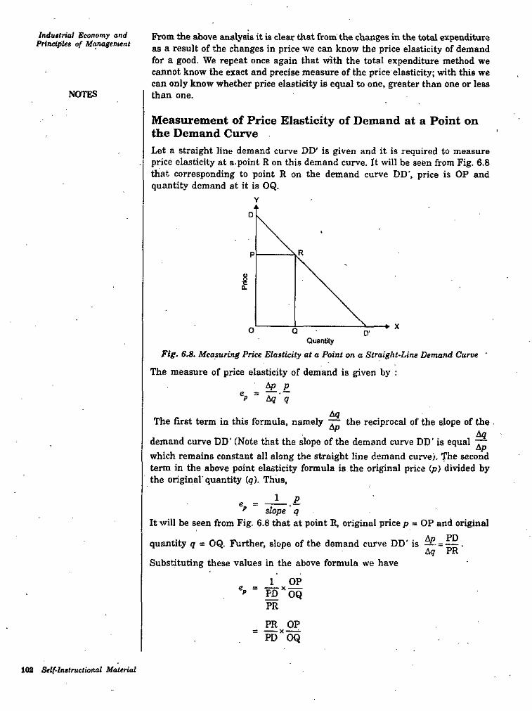
Induitrial Economy and Principles of Management
From the above analysis it is clear that from the changes in the total expenditure as a result of the changes in price we can know the price elasticity of demand for a good. We repeat once again that with the total expenditure method we cannot know the exact and precise measure of the price elasticity: with this we can only know whether price elasticity is equal to one, greater than one or less than one.NOTES
Measurement of Price Elasticity of Demand at a Point on the Demand CurveLet a straight line demand curve DD' is given and it is required to measure price elasticity at a. point R on this demand curve. It will be seen from Fig. 6.8 that corresponding to point R on the demand curve DD', price is OP and quantity demand at it is OQ.
D
RP
I0.
Xo Q O'Quantity
Fig. 6.8. Measuring Price Elasticity at a Point on a Straight-Line Demand Curve '
The measure of price elasticity of demand is given by :Ap p
% = Aq qAq
The first term in this formula, namely ^ the reciprocal of the slope of theAq
demand curve DD' (Note that the slope of the demand curve DD' is equal ~Apwhich remains constant all along the straight line demand curve). The second term in the above point elasticity formula is the original price (p) divided by the originaT quantity (q). Thus,
1 Pe’’ slope q
It will be seen from Fig. 6.8 that at point R, original price p « OP and original
Aq PRquantity q = OQ. Further, slope of the demand curve DD' is
Substituting these values in the above formula we have
1 OP PO’^OQPR
PO’^OQ
Self-Instructional Material
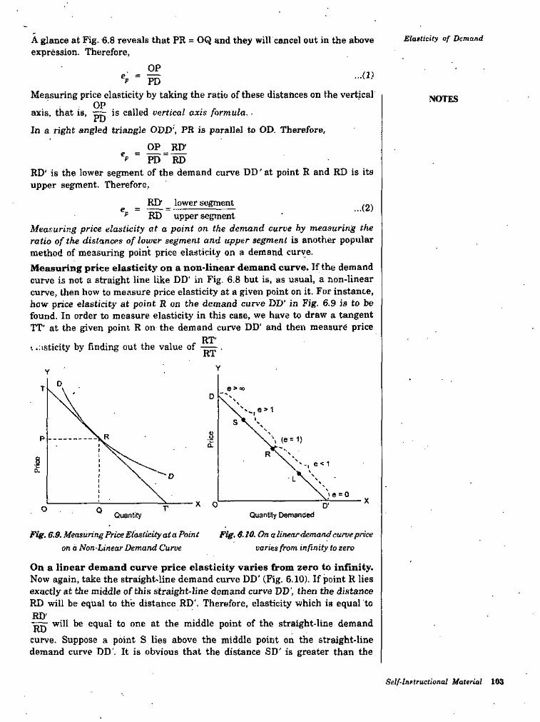
ElatCieity of DemandA glance at Fig. 6.8 reveals that PR = OQ and they will cancel out in the above expression. Therefore,
OP.M)~ PD
Measuring price elasticity by taking the ratio of these distances on the vertical OP is called vertical axis formula. •
NOTESaxis, that is,In a right angled triaagle ODD', PR is parallel to OD. Therefore,
OP RD’PD RD
RD' is the lower segment of the demand curve DD'at point R and RD is its upper segment. Therefore,
ep
ED* lower segment MD upper segment
Measuring price elasticity at a point on the demand curve hy measuring the ratio of the distances of lower segment and upper segment is another popular method of measuring point price elasticity on a demand curve.Measuring price elasticity on a non-linear demand curve. If the demand curve is not a straight line like DD' in Fig. 6.8 but is, as usual, a non-linear curve, then how to measure price elasticity at a given point on it. For instance, how price elasticity at point R on the demand curve DD' in Fig. 6.9 is to be found. In order to measure elasticity in this case, we have to draw a tangent TT' at the given point R on the demand curve DD' and then measure price
*. .asticity by finding out the value of
...(2)=
RT'RT
YY
TD
8PQ.
8-ce.
D'Q Quantity
Fig. 6.9. Measuring Price Elasticity at a Point on a Non-Linear Demand Curve
OQuanbty DemanCeC
Fig. 6.10. On a linear demand curve price varies from infinity to zero
On a linear demand curve price elasticity varies from zero to infinity. Now again, take the straight-line demand curve DD' (Fig. 6.10). If point R lies exactly at the middle of this straight-line demand curve DD', then the distance RD will be equal to the distance RD', Therefore, elasticity which is equal to
will be equal to one at the middle point of the straight-line demandcurve. Suppose a point S lies above the middle point on the straight-line demand curve DD’. It is obvious that the distance SD' is greater than the
RiyRD
Self-Inftructional Material 103
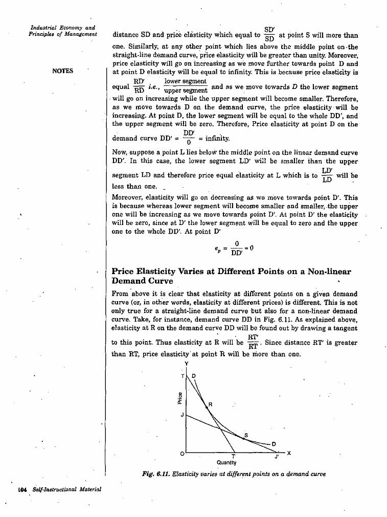
Industrial Economy and Principles of Management sudistance SD and price elasticity which equal to at point S will more thanSD
one. Similarly, at any other point which lies above the middle point on the straight-line demand curve, price elasticity will be greater than unity. Moreover, price elasticity will go on increasing as we move further towards point D and at point D elasticity will be equal to infinity- This is because price elasticity is
lower segmentNOTES
RD-equal and as we move towards D the lower segmenti.e..RD upper segmentwill go on increasing while the upper segment will become smaller. Therefore,as we move towards D on the demand curve, the price elasticity will be increasing. At point D, the lower segment will be equal to the whole DD', and the upper segment will be zero. Therefore, Price elasticity at point D on the
DD-demand curve DD' * = infinity.
Now, suppose a point L lies below the middle point on the linear demand cu^e DD'. In this case, the lower segment LD' will be smaller than the upper
LD’segment LD and therefore price equal elasticity at L which is to L̂Dless than one.Moreover, elasticity will go on decreasing as we move towards point D'. This is because whereas lower segment will become smaller and smaller, the upper one will be increasing as we move towards point D'. At point D' the elasticity will be zero, since at D' the lower segment will be equal to zero and the upper one to the whole DD'. At point D'
vrill be
^ = 0DD'
Price Elasticity Varies at Different Points on a Non-linear Demand CurveFrom above it is clear that elasticity at different points on a given demand curve (or, in other words, elasticity at different prices) is different. This is not only true for a straight-line demand curve but also for a non-linear demand curve. Take, for instance, demand curve DD in Fig. 6.11. As explained above, elasticity at R on the demand curve DD will be found out by drawing a tangent
to this point. Thus elasticity at R will be
than RT, price elasticity at point R will be more than one.
RT. Since distance RT' is greaterRT
T
8■ca
J
o T J'Quantity
Fig. 6.11. Elasticity varies at different points on a demand curve
104 Self-Instructional Material
Elasticity of DemandHow exactly it is, will be given by actual value which is obtained from dividing
RT' by RT- Likewise, price elasticity at point S will be given bySJ' is smaller than SJ, elasticity at S will be less than one. Again how exactly it is, Quantity will be found from actually dividing SJ' by SJ. It is thus evident
■ that elasticity at point S is less than that at point R on the demand curve DD. Similarly, elasticity at other points of the demand curve DD will be found to be different.
SJ'. BecauseSJ
NOTES
Comparing Price Elasticity of Two Demand CurvesHaving explained the concept of price elasticity of demand we will now explain how the compare elasticity on two demand curves. First, we take up the case of two demand curves with different slopes starting from a given point on the Y-axis. This case is illustrated in Fig. 6.12 where two demand curves DA and DB which have different slopes but are starting from the same point D on the Y-axis. Slope of demand curve DB is less than that of DA. Now, it can be proved that at any given price the price elasticity on these two demand curves would be the same. If price is OP, then according to demand curve DA, OL quantity of the good is demanded and according to demand curve DB, OH quantity of the good is demanded. Thus, at price OP the corresponding points on the twodemand curves are E and F respectively. We know that price elasticity at a
lower segmentpoint on the demand curve is equal to Therefore, the priceupper segment'
EA’elasticity of demand at point E on the demand curve DA is equal to the price elasticity of demand at point F on the demand curve DB is equal to
andED
EBFD'
Y
D
8•c0.
P
O H A Quantity
Fig. 6.12. fHomparing price elasticity on the two demand curves
L B
Now, take triangle ODA which is a right-angled triangle in which PE is parallel
is equal to PD. 'Thus, the price elasticity atto OA. It follows that in it’ ED
OPpoint E on the demand curve DA is equal to PDNow, in the right-angled triangle ODB, PF is parallel to OB. Therefore, in it
OPFB Thus, price elasticity of demand at point F on the demandis equal to PD‘FD
Self-Instructional Material 105
Industrial Economy and Principles,,0/ Management OPcurve DB i$ also equal to
demand on points E and F on the two demand curves respectively is equal to OP
that is, elasticities of demand at points E and F are equal PD though theslopes of these two demand curves are different. It follows therefore that the elasticity is not the same thing as slope. Therefore, price elasticity on two demand curves should nut be compared by considering slope alone.
. From above it is clear that price elasticity of
PD’NOTES
Comparing Price Elasticity on Two Intersecting Demand CurvesWe now take up the case of comparing price elasticity at o given price when the two demand curves intersect. In Fig. 6.13 we have drawn two demand curves AB and CD which intersect at point E. It will be noticed from the figure that demand curve CD is flatter than the demand curve AB. Now, it can be easily proved that at every price, on the flatter demand curye CD, price elasticity will be greater than that on the relatively steeper demand curve AB. For example at price OP, coiresponding to the intersecting, point E, using the vertical axis
OPformula, elasticity at point E on demand curve CD = ^. Similarly, elasticity
OP It will be seen from Fig. 6^13 thatIt A
because distance PC is less than the distance PA. Hence at the price
OP, elasticity is greater on the flatter demand curve CD, as compared to steeper demand curve AB. Likewise, it can be.shown at any other given price, elasticity of demand will be greater on th6 flatter demand curve CD as compared . to the steeper demand curve AB.
at point E on the demand curve AB <=
OP OPPC PA
•AC
cA
8I E £ p£ P
0o Q B D M, B DQuantity
Fig. 6.13. Comparirig Price Elasticity of Thio Intersecting Demand Curves
Quantity Demanded
Fig. 6.14. Comparing Price Elasticity of Two Parallel Demand Curves
Comparing Price Elasticity on Two Parallel Demand CurvesNow, we will comparc.the price elasticity at two parallel demand curves at a given price. This has been illustrated in Fig. 6.14 where two demand curves AB and CD are given which are parjdlel to each other. The two demand curves being parallel to each other implies that they have the same slope. Now, we can prove that at price OP price elasticity of demand on the two demand curves
106 Self-Instructional Material
Elasticity of DemandAB and CD is different. Now, draw a perpendicular from point R to the point P on Y-axis. Thus, at price OP the corresponding points on the two demand curves are Q and R respectively.The elasticity of demand on the demand curve AB at point Q will be equal to
and at point R on the demand curve CD it is equal toRC
Because in a right-angled triangle OAB, PQ is parallel to OB :
^ OP QA = PA
Hence, price elasticity at point Q on the demand curve
QB RD NOTESQA
Therefore
OPAB PARDAt point R on the demand curve CD, price elasticity is equal to = , BecauseRC
RD ^ OP ’ RC “ PCin the right-angled triangle OCD, PR is parallel to OD. Therefore
OPHence, on point R on the demand curve CD, price elasticity =PC
OPOn seeing the diagram it will be clear that.at point Q the price elasticity PA-
OPand at point R the price elasticity- PC
PC is greater than PA,are not equal to each other. Because
OPOPPAPC
.It is, therefore, clear that at point R on the demand curve CD the price elasticity is less than that at point Q on the demand curve AB. when the tw'O demand curves being parallel to each other have the same slope. It also follows that as the demand curve shifts to the right the price elasticity of demand at a given price goes on declining. Thus, as has been just seen, price elasticity at price OP on the demand curve CD is less than that on the demand curve AB.
DETERMINANTS OF PRICE ELASTICITY OF DEMANDWe have explained above the concept of price elasticity of demand and also how it is measured. Now an important question is what are the factors which determine whether the demand for a good is elastic or inelastic. The following
. are the mein factors which determine price elasticity of demand for a commodity. The Availability of Substitutes.' Of all the factors determining price elasticity of demand the availability of the number and kinds of substitutes for a commodity is the most important factor. If for a commodity close substitutes are available, its demand tends to be clastic. If the price of such a commodity goes up, the people will shift to its close substitutes and as a result the demand for that commodity will greatly decline. The greater the possibility of substitution, the greater the price elasticity of demand for it. If for a commodity substitutes are not available, people will have to buy it even when its price rises, and therefore its demand would tend to be inelastic.
Self-Instructional Material 107
Industrial Economy and . Principles of Management For instance, if the price of Cam pa Cola were to increase sharply, many consumers
. would turn to other kinds of cold drinks, and as a result, the quantity demanded of Campa Cola will decline very much. On the other hand, if the price ofCampa Cola falls, many consumers will change from other cold drinks to Campa Cola. Thus, the demand for Campa Cola is elastic. It is the availability of close substitutes that makes the consumers sensitive to the changes in the price of Campa Cola and this makes the demand for Campa Cola elastic. Likewise, demand for common salt is inelastic because good substitutes for common salt are not available. If the price of common salt rises slightly, the people would consume almost the same quantity of salt as before since-good substitutes are not available. The demand for common salt is inelastic also because people spend a very little part of their income on it and even if its price rises it makes only negligible difference in their budget allocation for the salt.The Proportion of Consumer’s Income Spent. Another important determinant of the elasticity of demand is how much it accounts for in consumer’s budget. In other words, the proportion of consumer’s income spent on a particular commodity also influences the elasticity of demand for it. The greater the proportion of income spent on a commodity, the greater will be generally its elasticity of demand, and vice versa. The demand for common salt, soap, matches and such other goods tends to be highly inelastic because the households spend only a fraction of their income on each of them. When the price of such a commodity rises, it will not make much difference in consumer’s budget and therefore they will continue to buy almost the same quantity of that commodity and, therefore, the demand for them will be inelastic. On the other hand, demand for cloth in a country like India tends to be elastic since households spend a good part of their income on clothing. If the price of cloth falls, it will mean great saving in the budget of many households and therefore they will tend to increase the quantity demanded of the cloth. On the other hand, if the price of cloth rise.s many households will not afford to buy as much quantity of cloth as before, and therefore, the quantity demanded of cloth will fall.The Number of Uses of a Commodity. The greater the number of uses to which a commodity can be put, the greater will be its price elasticity of demand. If the price of a commodity having several uses is very high, its demand will be small and it will be put to the most important uses and if the price of such a commodity falls it will be put to less important uses also and consequently its quantity demanded will rise significantly. To illustrate, milk has several uses.,If its price rises to a very high level, it will be used only for essential purposes such as feeding the children and sick persons. If the price of milk falls, it would be devoted to other uses such as preparation of curd, cream, ghee and sweets. Therefore, the demand for milk tends to be elastic.Complementarity Between Goods. Complementarity between goods or joint demand for goods also affects the price elasticity of demand. Households are generally less sensitive to the changes in price of goods that are complementary with each other or which are jointly used as compared to those goods which have independent demand or used alone. For example, for the running of automobiles, besides petrol, lubricating oil is also used. Now, if the price of lubricating oil goes up, it will mean a very small increase in the total cost of running the automobile, since the use of oil is much less as compared to other things such as petrol. Thus, the demand for lubricating oil tends to be inelastic. Similarly, the demand for common salt is inelastic, partly because consumers do not use it alone but along with other things.
NOTES
lOS Self-Instructional Material
It is worth mentioning here that for assessing the elasticity of demaind for a commodity all the above three factors must be taken into account. The three factors mentioned above may reinforce each other in determining the elasticity of demand for a commodity or they may operate against each other. The elasticity of demand for a commodity will be the net result of all the forces working on it. •Time and Elasticity. The element of time also influences the elasticity of demand for a commodity. Demand tends to be more elastic if the time involved is long. This is because consumers can substitute goods in,the long run. In the short run, substitution of one commodity by another is not so easy. The longer the period of time, the greater is the ease with which both consumers and businessmen can substitute one commodity for another. For instance, if the price of fuel oil rises, it may be difficult to substitute fuel oil by other types of fuels such as coal or cooking gas. But. given sufficient time, people will make adjustments and use coal or cooking gas instead of the fuel oil whose price ha's risen. Likewise, when the business firms find that the price of a certain material has risen, then it may not be possible for them to substitute that material by some other relatively chcatier one. But with the passage of time they can undertake research to find .substitute material and can redesign the product or modify the machinery cmnlo3'ed in the production of a commodity so as to economise in the use of the dearer material. Thereforci given the time, they can substitute the material whose price ha-s risen. We thus see that demand is generally more elastic in the long run than in the short run.
Slasticity of Demand
NOTES
IMPORTANCE OF THE PRICE ELASTICITY OF DEMANDThe concept of elasticity of demand plays a crucial role in the pricing decisions of the business firms and the Government when it regulates prices. The concept of price elasticity is also important in judging the effect of'devaluation of a currency on its export earnings. It has also a great use in fiscal policy because the Finance Minister has to keep in view the elasticity of demand when it considers to impose taxes on various commodities. We shall explain below the various uses, applications and importance of the elasticity of demand. Pricing Decisions by Business Firms. The business firms take into account the price elasticity of demand when they take decisions regarding pricing of the goods. This is because change in the price of a product will bring about a change in the quantity demanded depending upon the coefficient of price elasticity. This change,in quantity demanded as a result of, say a rise in price by a firm, will affect the consumer’s total expenditure and will therefore, affect the revenue of the firm. If the demand for a product of the firm happens to be elastic, then any attempt on. the part of the firm to raise the price of its product will bring about a fall in it.s total revenvie. Thus, instead of gaining from the increase in price, it will lose if the demand for its product happens to-be clastic. On the other hand, if the demand for the product of a firm happens to be inelastic, then the, increase in price by it will raise its total revenue. Therefore, for fixing a profit maximising price, the firm cannot ignore the price elasticity of demand for its product.Price elasticity of demand can be used to answer the following types of questions;
1. What will be the effect on sales if a firm decides to raise the price of its product, say by 5 per cent ?
Setf-InelrucUonal Material 109
Industrial Economy and Principles of Management
2. How Jarge a reduction in price of a product is required to increase sales, say by 25 per cent ?
It has been found by some empirical studies that business firms often fail to take elasticity into account while taking decisions regarding prices, or they give insufficient attention to the coefficient of price elasticity. No doubt, the main reason for this is that they don’t have'the means to calculate price elasticity for their product, since sufficient data regarding past prices and quantity demanded at those prices are not available. Even if such data are available, there arc difficulties of interpretation of it because it is not clear
- whether the changes in quantity demanded were the result of changes in price alone or changes in some other factors determining the demand. However, recently big corporate business firms have est.abli.sbed *^’eir research departments which estimate the coefficient of price elasticity trom the data concerning past prices and quantities demanded. Further, they are also using statistical techniques to isolate the price-effect on the quantity demanded from the effects of other factors.Uses in Economic Policy Regarding Price Regulation, Especially of Farm Products. Governments of many countries, especially United States of America, regulate the prices of farm products. This price regulation involves the increase in the prices of farm products, and this is done with the expectation that the demand for the farm products is inelastic. That the demand for farm products is inelastic in countries like USA has been found from empirical studies. By restricting supply in the market, Government succeeds in raising the price for the farm products. The demand for these products being inelastic, the quantity demanded does not fall very much and as a result the expenditure of the consumers on farm products increases, which raises the incomes of the agricultural cla.ss. If the demands for farm products were elastic, any rise in their price brought about by Government’s restricted supply of them, would have caused the decrease in the incomes of the agricultural class. Therefore, the crop restriction programme and keeping part of the crop off the market by the Government would never have been considered, had the demand for farm products been elastic rather than inelastic.Explanation of the ‘Paradox’ of Plenty. The concept of price elasticity of demand also, helps us to explain the so called ‘paradox of plenty’ in agriculture, namely, that a bumper crop reaped by the farmers br.'ngs a smaller total income to them. The fall in the income or revenue of the farmers as a result of the bumper crop is due to the fact that with greater supply the prices of the crops decline drastically and in the context of inelastic demand for them, the total expenditure on the crop output declines, bringing about fail in the incomes of the farmers. Thus, bumper crop instead of raising their incomes, reduces them. Therefore, in order to ensure that the farmers do not loss incentive to raise their production, they need to be assured certain minimum price by the Government. At that minimum price the Government should bo prepared to buy the crop from the farmers.Use in Intetmatioiial Trade. The concept of price elasticity of demand is also crucially important in the field of international economics. The Governments of the various countries have to decide about whether to devalue their currencies or not when their exports are stagnant and imports are mounting and as a result their balance of payments position is worsening. The effect of the devaluation is to raise the price of the imported eoods and to lower the prices of the exports. If the demand for a country’s exports is inelastic, the fall in the prices of exports
NOTES
110 Sclf-lnatTuttional Material
as a result of devaluation will lower their foreign exchange earnings rather than increasing them. This is because, demand being inelastic, as a result of the fall in prices quantity demanded of the exported products will increase very little and the country would suffer because of the lower prices. On the other hand, if the demand for a country's exports is elastic, then the fall in the prices of these exports due to devaluation will bring about a large increase in their quantity demanded which will increase the foreign exchange earnings of the country and will thus help in solving the balance of payments problem. Thus, the decision to devalue or not, depends upon the coefficient of the demand elasticity of exports.Likewise, if the objective of devaluation is to reduce the imports of a country, then this will be realised only when the demand for the imports is elastic. The imports will decline very much as a result of rise in their prices brought about by devaluation and the country will save a good amount of foreign exchange. On the other hand, if the demand for imports is inelastic, the increase in prices as a result of devaluation will adversely affect the balance of payments, because at higher prices of the imports and almost the same quantity of imports, the country would have to spend more on the imports than before. Importance in Fiscal Policy. The ela-‘!li''Hy of demand is also of gi'eat significance in the field of fiscal policy. The Finance Minister has to take into account elasticity of damand of the product on which he proposes to impose the tax if the revenue for the Government is to be increased. The imposition of an indirect tax, such as excise duty or sales rax, raises the price of a commodity. Now, if the demand for the commodity is elastic, the rise in price caused by the tax, will bring about a large decline in the quantity demanded and as a result the Government revenue will decline rather than increase. The Government can succeed in increasing its revenue by the imposition of commodity faxes only if the demand for the commodity is inelastic.The elasticity of demand also determines to what extent a tax on a commodity can be shifted to the consumer. Thus, the incidence of a commodity tax on the consumers depends on their elasticity of demand for the commodity. If the demand for a commodity is perfectly inelastic, the whole of the burden of the commodity tax will fall on the consumers. When a tax is imposed on a commodity, its price will rise. As in the case of perfectly inelastic demand, the quantity demanded for the commodity remains the same, whatever the price, the price will rise to the extent of the tax per unit. Therefore, the consumers will bear the whole burden of the tax in the form of a higher price they pay for the same quantity demanded.On the contrary, if the demand for a commodity is perfectly elastic, the inpositioi of the tax oh it will not cause any rise in price and, therefore, the whole burden of the tax will be borne by the manufacturers or sellers. When demand is neither perfectly inelastic, nor perfectly elastic, then respective burdens borne by the consumers and the producers will depend upon the elasticity of demand as well as on the elasticity of supply. We thus see that a Finance Minister cannot ignore elasticity of demand for products while levying taxes.
Elasticity of Demand
NOTES
CROSS ELASTICITY OF DEMANDVery often demands for two goods are so related to each other that when the price of any of them changes, the demand for the other good also changes, when its own price remains the same. Therefore, degree of responsiveness of
Self-Instructional Material 111
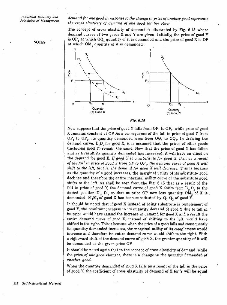
indusfrioJ Economy and Principles of Management demand for one good in response to the change in price of another good represents
the cross elasticity of demand of one good for the other.The concept of cross elasticity of demand is illustrated by Fig. 6.15 where demand curves of two goods X and Y are given. Initially, the price of good Y is OPj at which OQj quantity of it is demanded and the price of good X is OP at which OM^ quantity of it is demanded..NOTES
0.Dy
D'.
o•c 8^=\ \0.0.
p P?
Dy DyD',
XMO Q 020
Quantity {a) Good X Quantity
(b) GoodY
Fig. 6. IS
Now suppose that the price of good Y falls from OPj to OPj, while price of good X remains constant at OP. As a consequence of the fall in price of good Y from OP^ to OPj, its quantity demanded rises from OQj to OQj. In drawing the demand curve. for good X, it is assumed that the prices of other goods (including good Y) remain the same. Now that the price of good Y has fallen and as a result its quantity demanded has increased, it will have an effect on the demand for good X. If good Y is a substitute for good X, then as a result of the fall in price of good Y from OP to OP^, the demand curve of good X will shift to the left, that is. the demand for good X will decrease. This is because as the quantity of a good increases, the marginal utility of its substitute good declines and therefore the entire marginal utility curve of the substitute good shifts to the left. As shall be seen from the Fig. 6.16 that as a result of the fall in price of good Y, the demand curve of good X shifts from to the dotted position D’^ D'^ so that at price OP now less quantity OMj of X is , demanded. MjMj of good X has been substituted by Qj Qj of good Y,It should be noted that if good X instead of being substitute is complement of good Y, the resultant increase in its quantity demand of good Y due to fall in ' its price would have caused the increase in demand for good X and a result the
■ entire demand curve of good X, instead of shifting to the left, would have shifted to the right. This is because when the price of a good falls and consequently its quantity demanded increases, the marginal utility of its complement would increase and therefore its entire demand curve would shift to the right. With a rightward shift of the demand curve of good X, the greater quantity of it will be demanded at the given price OP.It should be noted again that in the concept of cross elasticity of demand, while the price o,^ one good changes, there is a change in the quantity demanded of another good.When the quantity demanded of good X falls as a result of the fall in the price of good Y, the coefficient of cross elasticity of demand of X for Y will be equal
112 Self-Instructional Material
Elasticiiy of Demandto the percentage change in the quantity demanded of good X in response to a given percentage change in the price of good Y. Therefore,Coefficient of cross elasticity of demand of X for Y
% change in the quantity demanded of X% change in the price of good Y . NOTES
xlOO'
X100 PyPy
<?, ^Py ^<ly ' P.Cp Stands for cross elasticity of demand of X for Y
stands for the original quantity demanded ofX Aq stands for change in quantity demanded of good X Pj, stands for the original price of good Y
stands for a small change in the price of good Y
where
Numerical ProblemLet us take an example. If the price of coffee rises from Rs. 4.50 per hundred grams to Rs. 5 per hundred grams and as a result the consumer's demand for tea increases from 60 hundred grams to 70 hundred grams, then the cross elasticity of demand of tea for coffee can be found out as follows :In the above example :
= 70 - 60 = 10 hundred grams = 60 hundred grams
Ap^ = Rs. 5 - 4.50 = 50 paise p^, = Rs. 4.50 = 450 paise
^ b. Px.
W 450 350’' 60
Cross elasticity of demand =
2
Substitute and Complementary GoodsAs we have seen in the example of tea and coffee above, when two goods are substitutes of each other, then as a result of the rise in price of one good, the quantity demanded of the other good increases. Therefore, the cross elasticity of demand between the two substitute goods is positive, that is, in response to the rise in price of one good, the demand for the other good rises. Substitute goods are also known as competing goods. On the other hand, when the two goods are complementary with each other just as bread and butter, tea and milk etc., the rise in price of one good brings about the decrease in demand for the other. Therefore, the cross elasticity of demand between the two complementary goods is negative. Therefore according to the classification based on the concept of cross elasticity of demand, goods X and Y are substitutes or complements according as the cross elasticity of demand is positive or negative.
Self-Instructional Material 113
Indiisiriai Economy and Principles of Management
The concept of cross elasticity of demand is very important in economic theory. The substitute and complementary goods, as we have seen above, are defined in terms of cross elasticity of demand- The goods between which cross elasticity of demand in positive are known as substitute goods and the goods between which cross elasticity of demand is negative are complementary goods. Besides, classification of various types of market structures is made on the basis of cross elasticity of demand. Thus, Professor Triffen has employed the concept of cross elasticity of demand in distinguishing the various forms of markets. Perfect competition is defined as that in which the cross elasticity of demand between the products produced by many firms in'it is infinite- Monoploy is said to exist when 'a producer produces a product the cross elasticity of demand for which with any other product is very low. In fact, the pure or absolute monopoly is sometimes defined as the production by a single producer of a product whose cross elasticity of demand with any other product is zero. Monopolistic competition is said to prevail in the market when a large number of firms produces those products between which cross elasticity of demand is large and positive, that is, they are close substitutes of each other.
NOTES
Importance of Cross Elasticity of Demand for Business Decision MakingThe concept of cross elasticity of demand is of great importance in managerial decision making for formulating proper price strategy. Multiproduct firms often use this concept to measure the effect of change in price of one product on the demand for other products. For example, Maruti Udyog Ltd. produces Maruti Vans, Maruti 800 and Maruti Esteem. These products are good substitutes of each other and therefore cross elasticity of demand between them is very high. If Maruti Udyog decides to lower the price of Maruti 800, it will significantly affect the demand for Maruti Vans and Maruti Esteem. So it will formulate a proper price strategy fixing appropriate price for its various products. Further, Gillete Company produces both razors and razor blades which are complements with high cross elasticity of demand. If it decides to lower the price of razors, it will greatly increase the demand for razor blades. Thus there is need for adopting a proper price strategy when it produces products with high positive or negative cross price elasticity of demand.Second, the concept of cross elasticity of demand is frequently used in defining the boundaries of an industry and in measuring interrelationship between industries. An industry is defined as a group of firms producing similar products that is, products with a high positive cross elasticity of demand. For example cross elasticity of demand between Maruti Esteem, Dawoo Ceilo, Opel Astra is positive and quite high. They therefore belong to the same industry (i.e., automobiles). It should be noted that because of interrelationship of firms and industries between which cross price-elasticity of demand is positive and high, any one cannot raise the price of its product without losing sales to other firms in the related industries.Farther, the concept of cross elasticity of demand is extremly used in the United States in deciding cases relating to Antitrust laws and monopolistic practices used by firms. It so happens that in order to reduce competition that one dominant firm producing a product with high cross elasticity of demand with the products of other firms tries to take over them and thereby establish a monopoly or different firms try to merge with each other to form a cartel to enjoy monopolistic profits. These actions are held illegal by Antitrust or
114 Self-Instructional Material
anti-monopoly laws. An interesting attempt was made in India by Coca-Cola. In 1995 when it returned to India following the adoption of policy of liberalisation. In order to reduce competition, Coca-Cola company purchased the firm producing Thums Up, Gold Spot, Limca which have high positive cross elasticity of demand with Coca-Cola and it further made efforts to take over ‘Pure Drinks’, the producer of Campa-Cola, another close substitutes but failed. If it had succeeded in its venture it could have significantly reduced competition. With this its competition would have been with other multinational rival firm Pepsi-Cola.
Elasticity of Demand
NOTES
INCOME ELASTICITY OF DEMANDAnother important concept of elasticity of demand is income elasticity of demand. Income elasticity of demand shows the degree of responsiveness of quantity demanded of a good to a small change in the income of consumers. The degree of response of quantity demanded to a change in income is measured by dividing the proportionate change in quantity demanded by the proportionate change in income. Thus, more precisely, the income elasticity of demand may be defined as the ratio of the percentage change in purchases of a good to a percentage change in income which induces the former.
% change in purchases of a good % change in income
Let Y stand for an initial income, AY for a small change in income, Aq for the initial quantity purchased, Aq for a change in quantity purchased as a result of a change in income and e,. for income elasticity of demand. Then,
Income elasticity =
^xlOO_ Aq ^ AY _ Aq Yg
= AY xlOOY
If, for instance, consumer’s weekly income rises from Rs. 300 to Rs. 320, his purchase of the good X increases from 25 units per week to 30 units, then his income elasticity of demand for X is:
-^xlOO 1-1 = 1x15 = 3
1 525
.300xlOO
15
Income elasticity of demand being zero is of great significance. Zero income elasticity of demand for a good implies that a given increase in income does not at all lead to any increase in quantity demanded of a good or expenditure on it. In other words, zero income elasticity signifies that quantities demanded of the good is quite unresponsive to changes in income.
Income Elasticity, Normal Goods and Inferior GoodsBesides, zero income elasticity is significant because it represents dividing line between positive income elasticity on the one side and negative income elasticity on the other. On the one side, when income elasticity is more than zero (that is, positive), then an increase in income leads to the increase in quantity demanded of the good. This happens in case of normal goods. On the other side of zero income elasticity are all those goods whose income elasticity is less
Self-Instructional Material ll5
JndustriaJ Economy and Principles of Management than zero (that is, negative) and in such cases increase in income will lead to
the fall in quantity demanded of the goods. Goods having negative income elasticity are known as inferior goods. Goods with positive income elasticity are called normal goods. We thus see that zero income elasticity is a significant value, for it helps us to distinguish normal goods from inferior goods.
NOTESIncome Elasticity, Luxuries and NecessitiesAnother significant value of income elasticity is unity. This is because when income elasticity of demand for a good is equal to one, then proportion of income spent on the good remains the same as consumer’s income increases. Income elasticity .of unity also represents a useful dividing line. If the income elasticity for a good is greater than one, the proportion of consumer’s income spent on the good rises as consumer’s income increase, that is, that good bulks larger in consumer’s expenditure as he becomes richer. On the other hand, if the income elasticity for a good is less than one, the proportion of consumer's income spent on it falls as his income rises, that is, the good becomes relatively less important in consumer’s expenditure as his income ri.ses. A good having mcome elasticity more tfian one and which therefore bulks larger in consumer’s budget as he becomes richer is called a luxury. A good with an income elasticity less than one and which claims declining proportion of consumer’s income as he becomes richer is called a necessity. It should, however, be noted that the definitions of luxuries and necessities on the basis of income elasticity may not conform to their definitions in Engligh dictionary because the dictionary's luxuries may be necessities and its necessities may be luxuries according to
. the above definition. But in economic theory it is useful to call the goods with income elasticity greater than one as luxuries and goods with income elasticity less than one as necessities.
Importance of Income Elasticity for Business FirmsThe concept of income elasticity is important for decision making both by business firms and industries. First, the firms producing products which have a high income elasticity have great potential for growth in an expending economy. For example, if for a firm's product income elasticity of demand is greater than one, it means that it will gain more than proportionately to the increase in national income. Thus firms which are producing products having high income elasticity are more interested in forecasting the level of aggregate economic activity (i.e., level of national income) because the demand for their products will greatly depend on the level of overall economic activity. Further, as seen above, the demand for luxuries is highly income elastic. Therefore, the demand for luxuries fluctuate very much during different phases of business cycles- During boom periods, demand for luxuries increase very much, and decline sharply during recessionary periods.On the other hand, the demand for products with low income elasticity will not be greatly affected by the fluctuations in aggregate economic activity. During booms the demand for their products will not increase much and during recessions it will not decrease sharply. Therefore, the firms with low income elasticity for their products would not be much interested in forecasting future business activity. Remember it is generally necessities for which demand is not much income elastic. However, there is one good thing for the firms which face low income elasticity. They are to a good extent recession-proof. In the periods of recession, their incomes do not fall to the extent of decline in aggregate
119 Self-Instructionai Materiel
Elasticity of Demandincome. Of course, to share the benefits of increasing national income firms currently producing products with low income elasticity would try to enter the industries demand for whose products is highly income elastic as this would ensure better growth opportunities.The knowledge of income elasticity of demand also plays.a significant role in designing marketing strategies of the firms. If income of people is an important determinant of demand for a product, the firms producing product with high income elasticity of demand will be located in those areas or set up their sales outlets in those cities or regions where incomes are increasing rapidly. Besides, the firms will direct their advertising campaigns and- other sales production actmties to those segments of people whose income is high and also increasing rapidly. This is to ensure higher growth of sales of their products.The concept of income elasticity of demand shows clearly why fanners income do not rise equal to that of urban people engaged in manufacturing industries. Income elasticity of demand for agricultured products such as foodgrains is less than one. This implies that it is difficult for the farmers’ income from agriculture to increase in proportion to the expanding national income. Thus farmers cannot keep up with the urban people who derive their incomes from industries producing goods with high income elasticity of demand.
NOTES
Self-Instructional Jdaterial 117
InduBtrial Keonomy and Principles of Management
STUDENT ACTIVITy
1. What is meant by Elasticity of Demand ?
2. Discuss various concepts of Demand Elasticity.
118 Self-Insiructional Material
Elasticity of DemandSUMMARY
« • When the price of a good falls, its. quantity demanded rises and when the price of its rises, its quantity demanded falls. This is generally known as law of demand.
• Demand for a good is said to be elastic if the price elasticity of demand for'it is greater than one. Similarly, the demand for a good is called inelastic if. price elasticity of demand for it is less than one.
• The business firms take into account the price elasticity of demand when they take decisions regarding pricing of the goods.
• Degree of responsiveness of demand for one good in response to the change in price of another good represents the cross elasticity of demand of one good for the other.
• A good having income elasticity more than one and which therefore bulks larger in consumer’s budget as he becomes richer is called a luxury. A good with an income elasticity less than one and which claims declining proportion of consumer’s income as he becomes richer is called a necessity.
NOTES
IWEVIEW E3CERCISES1. Write a detail note on Measurement of Price Elasticity.'2. What are the determinants of Price Elasticity of Demand ?3. Discuss the importance of Price Elasticity of Demand.4. Discuss Cross Elasticity of Demand.5. Discuss the importance of Cross Elasticity of Demand.'
Self-lnstructionai Material 119
Industrial Economy'and Principles of Management UNIT 7 INDIFFERENCE CURVE
ANALYSISNOTES
★ STRUCTURE ★□ Indifferennce Curve Approach□ What are Indifference Curves? a Marginal Rate of Substitution□ PropertiesoflndifferenceCurves□ Budget Line□ Consumer’s Equilibrium ; Maximising Satisfaction□ Income Consumption Curve and Engel Curve□ Substitution Effect
□ Price Effect; Price Consumption Curve□ Decomposing Price Effect into Income and Substitution Effects□ Price-Demand Relationship ; Deriving Law of Demand□ Derivation of Individual’s Demand Curve from Indifference Curve Analysis
Superiority of Indifference Curve Analysis• □ Critique of Indifference Curve Analysis
A popular alternative theory of consumer’s demand is the Indifference Curve Analysis which forms the subject-matter of the present chapter. The technique of indifference curves was first of all invented by a classical economist Edgeworth but he used it only to sliow the possibilities of exchange between two persons and not to explain consumer’s demand.Two English economists, J.R. Hicks and R.G.D. Allen in their now well-known paper ‘A Reconsiderofion of the Theory, of Value’ severely criticised Marshall’s utility analysis based upon cardinal measurement of utility and put forward the indifference curve approach based upon the notion of ordinal utility to explain consumer’s behaviour. In 1939 Hicks reproduced the indifference curve theoiy of consumer’s demand in his book "Value and Copitcf’modifying somewhat the version of the original paper.
INDIFFERENCE CURVE APPROACHIndifference curve method has been evolved to supersede the marginal utility analysis of demand which was discussed in the last chapter. The indifference curve method seeks to derive all rules and laws about consumer’s demand that are derivable from the cardinal utility analysis. At the same time the inventors and supporters of new method contend that their analysis is based on fewer and more reasonable assumptions. The indifference curve analysis has, however,
Ut A^utruefiono/ Ualerial
lndiffer,’nce Curve AnalynUretained some of the assumptions of Marshall’s cardinal utility analysis. Thus, the indifference cur%’i) approach, like the old cardinal utility approach, assumes that the consumer possesses ’complete information' about all the relevant aspects of economic environment in which ho finds himself. For example, the prices of goods, the markets in which they are available, the satisfaction to bo obtained from them etc., are all known to the consumer, hufiher, it iff assumed that the consumer acts rationally in the sense that, given the prices of goods and the money income, he will choose the combination from among the various possible combinations that gives him maximum satisfaction. Moreover, the assumption of‘continuity’has also been retained by Hicks-Allen indifference curve method. Continuity assumption means that the consumers are capable of ordering or ranking all conceivable combinations of goods according to the satisfaction they yield.ITro fundamental approach of indifference curve analysis is that it has abandoned the concept of cardinal utility and instead has adopted the concept of ordinal utility. According to the supporters of the indifference curves theory, utility is, a psychic entity and it cannot therefore be measured in quantitative cardinal terms. In other words, utility being a psychological feeling is not quantifiable. The concept of cardinal utility, according to the exponents of the indifference curve theory, is therefore untenable. On the other hand, the assumption of ordinal utility, according to them, is quite reasonable and-realistic. The ordinal utility implies that the consumer is capable of simply ‘comparing the different levels of satisfaction'.Tn other words, according to the ordinal utility hypothesis, while the consumer may not be able to indicate the exact amounts of utilities that he derives from commodities or any combination of them, but he is capable of judging whether the satisfaction obtained from a good or a combination of goods is equal to, lower than, or higher than another.For deriving the theory of consumer’s behaviour, it is sufficient to assume that the consumer is able to rank his preferences consistently.. Thus, the basis of indifference curve analysis of demand is the preference-indifference hypothesis. This means that if the consumer is presented with a number of various combinations of goods, he can order or rank them in ‘scale of preferences’. If the various combinations are marked A, B, C, D, E, etc., the consumer can tell whether he prefers A to B, or B to A. or is indifferent between them. Similarly, he can indicate his preference or indifference between any other pair of combinations. The. concept of ordinal utility implies that the consumer cannot go beyond stating his preference or indifference. In other words, if a consumer happens to prefer A to B, he cannot tell by how much he prefers A to B. Thus, under ordinal utility hypothesis, the consumer cannot tell the ‘quantitative differences’ between various levels of satisfaction; he can simply compare them ‘qualitatively’, that is, he can merely judge whether one level of satisfaction is higher than, lower than or equal to another. Further, according to the supporters of indifference- curve method, by ‘how much’ one combination of goods is preferred to another is not even needed for deriving laws concerning consumer’s behaviour. It is sulTicient to assume that the consumer is able to tell whether one combination of goods gives him greater, equal, or less satisfaction than another.It may b6 noted that the consumer formulates his.scale of preferences independently of the market prices of goods keeping in view only the satisfaction which he hopes to get from various combinations of goods. In consumer’s scale of preferences some combinations will occupy the same place, i.e., the consumer will be indifferent among them. Combinations occupying a higher place in the scale will be preferred to the combinations occupying lower places in the scale.
NOTES.
Self-Instructional Material 121
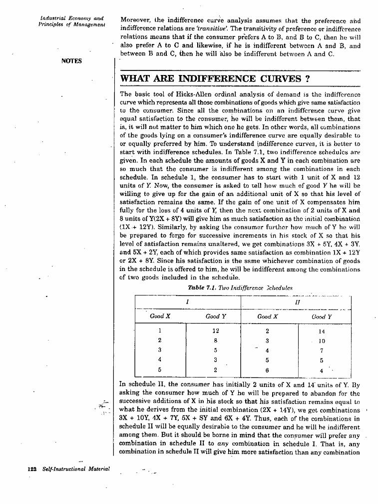
Industrial Economy and Principles of Management Moreover, the indifference curve analysis assumes that the preference and
indifference relations are ‘transitive’. The transitivity of preference or indifference relations means that if the consumer prefers A to B, and B to C, then he will also prefer A to C and likewise, if he is indifferent between A and B, and between B and C, then he will also be indifferent between A and C.
NOTES
WHAT ARE INDIFFERENCE CtIRVES ?The basic tool of Hicks-Allen ordinal analysis of demand is the indifference curve which represents all those combinations of goods which give same satisfaction to the consumer. Since all the combinations on an indifference curve give equal satisfaction to the consumer, he will be indifferent between them, that is, it will not matter to him which one he gets. In other words, all combinations of the goods lying on a consumer’s indifference curve are equally desirable to or equally preferred by him. Tb understand indifference curves, it is belter to start with indifference schedules. In Table 7.1, two indifference schedules are given. In each schedule the amounts of goods X and Y in each combination are so much that the consumer is indifferent among the combinations in each schedule. In schedule 1, the consumer has to start with 1 unit of X and 12 units of Y. Now, the consumer is asked to tell how much of good Y he will be willing to give up for the gain of an additional unit of X so that his level of satisfaction remains the same. If the gain of one unit of X compensates him fully for the loss of 4 units of Y then the next combination of 2 units ofX and 8 units of Y(2X + 8Y) will give him as much satisfaction as the initial combination (IX + 12Y). Similarly, by asking the consumer further how much ofY he will be prepared to forgo for successive increments in his stock of X so that his level of satisfaction remains unaltered, we get combinations 3X +- 6Y, 4X + 3Y, and 5X + 2Y, each of which provides same satisfaction as combination IX + 12y or 2X + 8Y. Since his satisfaction is the same whichever combination of goods in the schedule is offered to him, he will be indifferent among the combinations of two goods included in the schedule.
Table 7.1. Tivo Indifference jchedules
I II
GoodX Good Y Good X Good Y
1 12 2 142 8 3 103 5 44 3 5 55 2 6 4
In schedule II, the consumer has initially 2 units of X and 14'units of Y. By asking the consumer how much of Y he will be prepared to abandon for the successive additions of X in his stock so that his satisfaction remains equal to what he derives from the initial combination (2X + 14Y). we get combinations ' 3X + lOY, 4X + 7Y, 5X + SY and 6X + 4Y. Thus, each of the combinations in schedule II will be equally desirable to the consumer and he will he indifferent among them. But it should be borne in mind that the consumer will prefer any . combination in schedule II to any combination in schedule I. That is, any combination in schedule II will give him more satisfaction than any combination
.r—
122 Self-Instructional Material
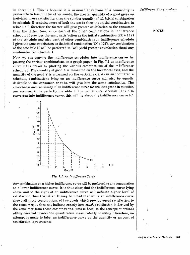
Indifference Curve Aiialy>>if<in shcedule I. This is because it is assumed that more of a commodity is preferable to less of it (in other words, the greater quantity of a good gives an individual more satisfaction than the smaller quantity of it). Initial combination in schedule II contains more of both the goods than the initial combination in schedule I, therefore the former will give greater satisfaction to the consumer than the latter. Now, since each of the other combinations in indifference schedule II provides the same satisfaction as the initial combination (2X + IdY) of the schedule and also each of other combinations in indifl'erence schedule I gives the same satisfaction as the initial combination (IX + 12Y), any combination of the schedule II will be preferred to (will yield greater satisfaction than) any combination of schedule I.Now, wc can convert the indifference schedules into indifference curves by plotting the various combinations on a graph paper. In Fig. 7,1 an indifference curve IC is drawn by plotting the various combinatiOn.s of the indifference schedule I. The quantity of good X is measured on the horizontal axis, and the quantity of the good Y is measured on the vertical axis. As in an indifference schedule, combinations lying on an indifference curve will also be equally desirable to the consumer, that is, will give him the same satisfaction. The smoothness and continuity of an indifference curve means that goods in question are assumed to be perfectly divisible. If the indifference schedule II is also converted into indifference curve, this will lie above the indifference curve IC.
NOTES
13-
1211 -
10-
iO 7-
6-54-
3-
2--
1-
O1-2 3 5 6 7-34
GoodX
Fig. 7.1. An Indifference Curve
Any combination on a higher indifference curve will be preferred to any combination on a lower indifference curve. If is thus clear that the indifference curve lying above and to the right of an indifference curve will indicate higher level of satisfaction than the latter. It may be noted that while an indifference curve shows all those combinations of two,goods which provide equal satisfaction to the consumer, it does not indicate exactly how much satisfaction is derived by the consumer from those combinations. This is because the concept of ordinal utility does not involve the quantitative measurability of utility. Therefore, no attempt is made to label an indifference curve by the quantity or amount of satisfaction it represents.
Self-Instructional Material 123
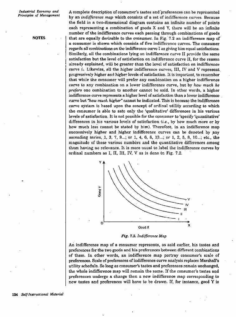
Industrial Economy and Principles of Management
A complete description of consumer’s tastes and preferences can be represented by an indifference map which.consists of a set of indifference curves. Because the field in a two-dimensional diagram contains an infinite number of points each representing a combination of goods X and Y, there will be an infinite number of the indifference curves each passing through combinations of goods that are equally desirable to the consumer. In Fig. 7.2 an indifference map of a consumer is shown which consists of five indifference curves. The consumer regards all combinations on the indifference curve I as giving him equal satisfactions. Similarly, all the combinations lying on indifference curve II provide the same satisfaction but the level of satisfaction on indifference curve II, for the reason already explained, will be greater than the level of satisfaction on indifference curve L. Likewise, all the higher indifference curves, III, IV and V represent progressively higher and h^her levels of satisfaction. It is important, to remember that while the consumer will prefer any combination on a higher indifference curve to any combination on a lower indifference curve, but by how much he prefers one combination to another cannot be said. In other words, a higher indifference curve represents a higher level of satisfaction than a lower indifference curve but “how much higher” cannot be indicated. This is because the indifference curve system is based upon the concept of ordinal utility according to which the consumer is able to sate only the ‘qualitative' differences in his various levels of satisfaction- It is not possible for the consumer to ‘specify ‘quantitative' differences in his various levels of satisfaction li.e., by how much more or by how much less cannot be stated by him). Therefore, in an indifference map successively higher and higher indifference curves can be denoted by any ascending series, 1, 3, 7. 9...; or 1, 4, 6, 8. 13...; or 1, 2, 5, 8, 10...; etc., the magnitude of these various numbers and the quantitative differences among them having no relevance. It is more usual to.label the indifference curves by ordinal numbers as I, II, III, IV, V as is done -in Fig. 7.2.
NOTES
>-
0 XGoodX
Fig. 7.2. Indifference Map
An indifference map of a consumer represents, as said earlier, his tastes and preferences for the two goods and his preferences between different combinations of them. In other words, an indifference map portray consumer’s scale of preferences. Scale of preferences of indifference curve analysis replaces Marshall’s utility schedule. So long as consumer’s tastes and preferences remain unchanged, the whole indifference map will remain the same. If the consumer's tastes and preferences undergo a change then a new indifference map corresponding to new tastes and preferences will have to be drawn. If, for instance, good Y is
124 Self-Instructional Material
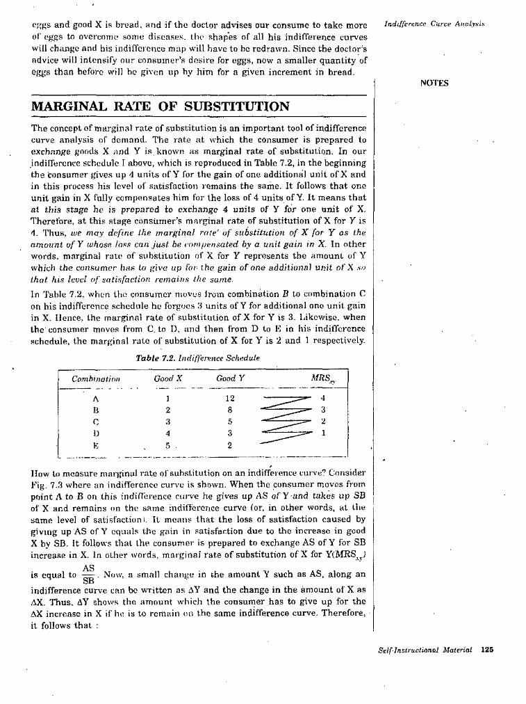
o;;f;s and good X is broad, and if Ihc doctor advises our consume to take more of eggs to overcome some diseases, the shapes of all his indifference curves will change and his indifference map will have to be redrawn. Since the doctor’s advice will intensify our consumer’s dosii'e for eggs, now a smaller quantity of eggs than before will he given up hy him for a given increment in bread.
Indifference Citree Analysis
NOTES
MARGINAL RATE OF SUBSTITUTIONThe concept of marginal rale of substitution is an important tool of indifference curve analysis of demand. The rate at which the consumer is prepared to (ucchnnge goods X and Y is known as marginal rate of substitution. In our .indifference schedule I above, which is reproduced in Table 7.2, in the beginning the consumer gives up d units of Y for the gain of one additional unit ofX and in this process his level of satisfaction l emains the same. It follows that one unit gain in X fully compensates him for the loss of 4 units of Y. It means that at this stage he is prepared to exchange 4 units of Y for one unit of X. Therefore, at this stage consumer's marginal rate of substitution of X for Y is 4. Thus, we may define Ike. marginal rate' of substitution of X for Y as the amount of Y whose loss can just be l ornpensated by a unit gain in X. In other words, marginal rate of substitution of X for Y represents the amount of Y which the consumer has to give up for the gain of one additional unit of'X so that his level of satisfaction remains the same.In Table 7.2, when the consumer moves Irom combination B to combination C on his indifference schedule he forgoes 3 units of Y for additional one unit gain in X. Hence, the marginal rate of substitution of X for Y is 3. Likewise, when the consumer moves from C, to D, and then from D to K in his indifference schedule, the marginal rate of substitution of X for Y is 2 and 1 respectively.
Table 7.2. Indifference Schedule
MRSGoad yComhinatiiifi Good X
12 41A8 3B 2
2.3 5C30 142E 5
How to measure marginal rate ol'substitution on an indiffei ence cuive? Consider Fig. 7.3 where an indifference curve is shown. When the consumer moves from point A to B on this indifference curve he gives up AS of Y-and lakes up SB of X and remains on the same indifference curve (or, in other words, at the same level of satisfactioni. It means that the loss of satisfaction caused by giving up AS ofY equals the gain in satisfaction due to the increase in good X by SB. It follows that the consumer is prepared to exchange AS of Y for SB increase in X. In oLlier words, marginal rate of substitution of X for Y(MRS^,1
AS Now, a small change in the amount Y such as AS, along anis equal to SBindifference curve can be written as AY and the change in the amount of X asAX. Thus. AY shows the amount which the consumer has to give up for the AX increase in X if he is to remain on the same indifference curve. Therefore,it follows that :
Self-Jnstruclional Material 12S
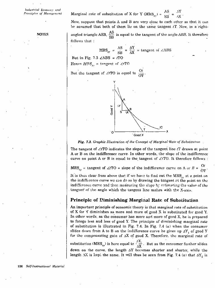
Indui^frinl liciiiKiiiiy unci I’riiiciii/rs of AS _ .\Y
SH' " .AX ■Now, suppose that points A and B aro very close to ouch other so that it can ho assumed that both of them lie on the same tangent IT. Now, in a right-
ASangled triangle ASB, —- is equal to the tangent of the angle ABS. It therefore oJ>
follows that :
Marginal i-atc of substitution of X for Y (MRS,,,) =XV
NO'IKS
AS _ AY S B " AXMRS„ ^
But in Fig. 7.3 ZABS = tl’O Hcnrn ~ tangent of /'.fTO
; = tangent of ZABS
OjBut the tangent of ZtTO is equal to --
Y
t
>oO
O' Good X
Fig. 7.3. Graphic Illustration of the Concept of Marginal 'Rate of Siihstiniliiw .
The tangent of ZtTO indicates the slope of the tangent lino iT drawn at point A or B on the indifference curve. In other words, the slope of the indifference curve on point A or B is equal to the tangent of ZtTO. It therefore follows :
OlMRS^^, = tangent of ZtTO = slope of the indifference curve on A or B .
It is thus clear from above that if we have to find out the MR9^. at a.point on the indifference curve wo can do so by drawing the tangent at the point on the indifference curve and then measuring the slope by "stima'ing the value of the
. tangenf of the angle which the tangent line makes with the X-axis.
Principle of diminishing Marginal Rate of SubstitutionAn important principle of economic theory is that marginal rate of substiiutioii of X for Y diminishes as more and more of good X is substituted for good Y In other words, as the consumer has more and more of good X, he is prepared to forego less and less of good Y. The principle of diminishing marginal rate of substitution is illustrated in Fig. 7,4. In Fig. 7.4 (a) when the consumer slides down from A to B on the indifference curve he gives up AYj of good Y for the compensating gain of aX of good X. Therefore, the marginal rate of
aysubstitution (MRS^^,,) is hero equal to . But as the consumer fur-lher slidesdown on the curve, the length AY becomes shorter and shorter, while the length AX is kept the same. It will thus be seen from Fig. 7.4 (a) that aYo, is
126 Self-Instructional Material
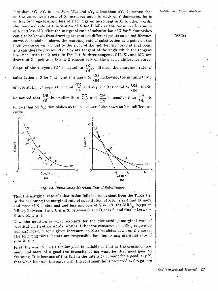
less than AY,; aY^ is loss than AY,: and AY_, is less than AYj. ll means that as the consumer’s stock o1'X increases and his stock of Y decreases, he is willing to forego less and loss of Y for a given increment in X. In other words, the marginal rate ol' substitution of X for Y falls as the consumer has more of X and less of Y. That the marginal rate of substitution of X for Y diminishes can also be known from drawing tangents at different points on an indifference curve, /is explained above, the marginal rate of substitution at a point on the indilference cui vo is equal to the slope of the indifference curve at that point and can therefore be- lound out by ate tangent of the angle which the tangent line made with the X-axis. In Fig. 7,4 (fcl three tangents GH, KL and MN are drawn at the points 1', Q and K respectively on the given indifference curve.
Indifference Curve Analysis
NOTES
Slope of the tangent Gll is equal to . Hence, the marginal rate of
OGsubstitution of X for Y at point i' is equal tc------Likewise, the marginal rateOH
OK“ .and at rmn' R is equal to . It willof substilwtif.n at point Q ir. equalOL ON
OKOK and OM is smaller than . It-- is smaller thanbe noticed that OLOL oi: ONfollows that ivlllS,,:. diminishes as tht. col. •.is,.ier slides down on his indifference curve.
YY
G
K
>>• oo
MO
\Y5 -JJ1C
XX oo'" NH LGooc X ,Good X
ia)(t»
Fig. 7.4. Diminishing Marginal Rate of Substitution
That the marginal rate of substitution falls is also evident from the Table IM. In the beginning the marginal rate of substitution of X for Y is 4 and as more and more ofX is obtained and les,s and less of Y is left, the MRS^,, keeps on falling. Between B and C it is 3; between C and D, it is 2; and final!: between !.■* and E, it is 1.Now, the question is what accounts for the diminishirg marginal rale of substitution. In other words, why is it that the consumer i-- -vilLr.g to give up U-S5 and Ic*-:The folln>>dng three factors are responsible for diminishing marginal rate of subsiitutidn.First.'the wai.l for a particular good is more and more of a good the intensity of his want for that good goes on declining. It is because of this fall in the intensity of want for a good, say X, that when its stock increasis with the consumer, he is prcpHrrt to forego less
c.r V for a gi’-en incremer’l in X as he slides down on the curve.
..utiable so that as the consumer has
Self Instructional Material 127
InduKtrial Econnmy and Principtex of Moiiageincnl
and less of good Y for every increment in X. In the beginning, when the consumer’s stock of good Y is relatively large and his stock of good X is relatively small, consumer’s marginal significance for good Y is low, while his 'marginal significance for good X is high. Owing to higher marginal significance of good X and lower marginal significance of good Y in the beginning the consumer will be willing to give up a larger amount of Y for a unit increase in good X. But as the stock of good X increases and intensity of desi?-e for it falls, his marginal significance of good X will diminish and on the other hand, as the stock of good Y decreases and the intensity of desii e for it increases, his marginal significance for good Y will go up. As a result, therefore, as the individual substitutes more and more of A for Y, he is prepared to give up less and less of Y for a unit increase in X.The second reason for the decline in marginal rate of sfibstitution is that the goods aru irnpei fecC substitutes of each other. If two goods are perfect substitutes of each other, then they are to bo regarded as one and the same good, and therefore increase in the quantity of one and decrease in the quantity of the other would not make any difference in the marginal significance of the goods. Thus, in case of perfect substitutability of goods, the increase and decrease will he virtually in the same good which cancel out each other and therefore the marginal rate of substitution remains the same and does not decline.Thirdly, the principle of diminishing marginal rale of substitution will hold good only if the increase in the quantity of one good does not increase the want satisfying power of the other. If with the increase in the stock of good X, the want satisfying power of good ; increases, then greater and greater amount of good Y will be required to he given up for a unit increase in good X so that consumer’s satisfaction remains the same.
NOI'KS
PROPERTIES OF INDIFFERENCE CURVESWe now turn to discuss the properties or attributes which the indifference curves normally possess. It will be useful if we first mention the assumptions about the psychology ol' the consumci’. which are generally made (at least implicitly) in indifference curve analysis.
More of a commodity is better than less. It is assumed that the consumer will always prefer a larger amount of a good to a smaller amount of that good, provided that the other goods at his disposal remains unchanged. This is a very reasonable and realistic assumption. This assumption implies that the consumer is not over-.supplied with any good. When a consumer is over-supplied or over-satiated with one good, he will prefer a smaller quantity of that good to the larger quantity. It is thus assumed that the consumer has not yet reached the point of satiety in the consumption of any good. This assumption is therefore known as nan-satiety assumption.
Preferences or indifferences of a consumer are transitive. Suppose there are three combinations of two goods ; A, B and C. If the is indifferent between A and H and also between B and C, it is then assumed that he will be indifferent between A and C too. This condition implies that consumer’s tastes are quite consistent. This assumption is kno%vn as assumption of transitivity.
Diminishing marginal rate of substitution. In indifference curve analysis principle of.diminishing marginal rate of substitution is assumed. In
1.
2.consumer
3.
128 Instructional Material
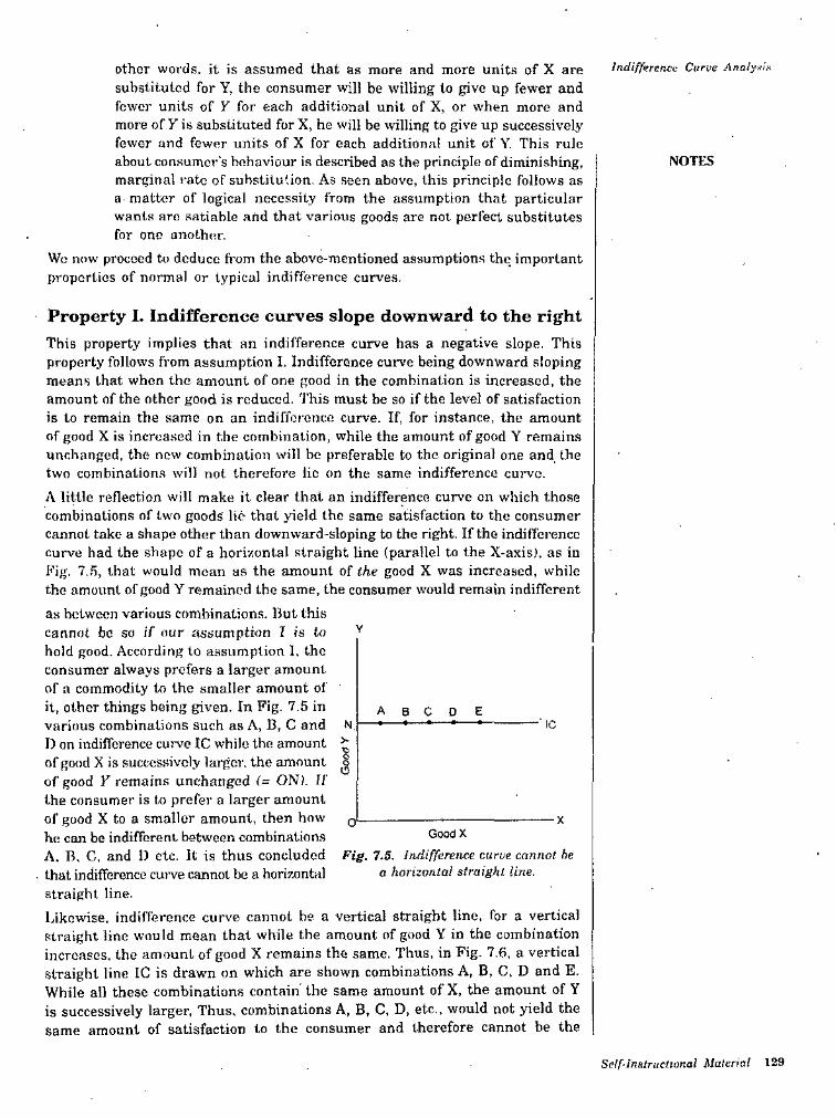
Indifference Curve Anolyr-'isother words, it is assumed that as more and more unit.s of X are substituted for Y, the con.sumer will be willing to give up fewer and fewer units of Y for each additional unit of X, or when more and more of Yis substituted for X, he will be willing to give up successively fewer and fewer units of X for each additional unit of Y. This rule about consumer's behaviour is described as the principle of diminishing, marginal rate of substiluiion. As seen above, this principle follows as a matter of logical necessity from the assumption that particular wants are .satiable and that various goods are not perfect substitutes for one anc)th<‘r.
Wo now proceed to deduce from the above-mentioned assumptions the. importantpropertios of normal or typical indifference curves.
NOTES
Property 1. Indifference curves slope downward to the rightThis property implies that an indifference curve has a negative slope. This property follows from assumption I. Indifference curve being downward sloping means that when the amount of one good in the combination is increased, the amount of the other good is reduced. This must be so if the level of satisfaction is to remain the same on an indiffotonce curve. If, for instance, the amount of good X is increased in the combination, while the amount of good Y remains unchanged, the new combination will be preferable to the original one and the two combination.s will not therefore lie on the same indifference curve.A little reflection will make it clear that an indifference curve on which those combinations of two goods lie that yield the same satisfaction to the consumer cannot take a shape other than downward-sloping to the right. If the indifference Curve had the shape of a horizontal straight line (parallel to the X-axis), as in Fig, 7..'5, that would moan as the amount of the good X was increased, while the amount of good Y remained the same, the consumer would remain indifferentas between various combinations. But this cannot be so if our assumption I is to hold good. According to assumption 1, the consumer always prefers a larger amount of a commodity to the smaller amount of it, other things being given. In Fig. 7.5 in various combinations such as A, B, C and N. - D on indifference curv'o IC while the amount ^ of good X is successively larger, the amount 8 of good y remains unchanged t= ON). W the consumer is to prefer a larger amount of good X to a smaller amount, then how q_ he can be indifferent between combinations
AbodeIC
GoodX
A. B, C, and 1) etc. It is thus concluded Fig. 7.5. Indifference curve cannot hea horizontal straight line.■ that indifference curve cannot be a horizontal
straight line.Likewise, indifference curve cannot be a vertical straight line, for a vertical straight line would mean that while the amount of good Y in the combination increases, the amount of good X remains the same. Thus, in Fig. 7.6, a vertical straight line IC is drawn on which arc shown combinations A, B, C. D and E. While ail these combinations contain the same amount of X, the amount of Y is successively larger, Thus, combinations A, B, C, D, etc., would not yield the
amount of satisfaction to the consumer and therefore cannot be thesame
Self-Instructional Material 129
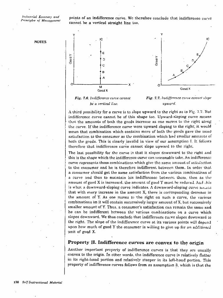
Iiiilii.iirial Econniny and l’•■inciptl'x n/ Mniitificinent points of an indifference curve. Wc therefore conclude that indifferenco eutvo
cannot be a vertical straight line too.
Y1C. 1CNOTKS /
/E> >-T3D tj
oO o
OC
B
A
O X ' OGoodXGoodX
Fin. 7.6. Indifference curve cannot be a vertical line.
Fig. 7.7. indifference curve, cannot slope upward.
A third pos-sibility for a curve is to slope upward to the right as in Fig. 7.7. But indifferenco curve cannot be of this shape too. Upward-sloping curve means
• that the amounts of both (he goods increase as one moves to the right along the curve. If the indifference curve were upward sloping to the right; it would mean that combination which contains more of both the goods gave the same satisfaction to the consumer as the combination which had smaller amounts of both the goods. This is clearly invalid in view of our assumption I. It foIiow.s therefore that indifference curve cannot slope upward to the right.The last possibility for the curve is that it slopes downward to the right and this is the shape which the indifference curve can reasonable lake. An indifference curve represents those combinations which give the same amount of oatisfaction to the consumer and he is therefore indifferent between them. In ordei' that, a consumer should get the same .satisfaction from the various combinations of a curve and thus to maintain his indifference between them, then as the amount of good X is increased, the amount of good Y must be reduced. And ibis is what a downward-sloping curve indicates. A downward-sloping curve nican.s that with every increase in the amount X, there is corresponding decrease in the arr*ounl of Y, As one moves to 'the right on such a curve, the various combinations bn it will contain successively larger amount of X, but successively smaller amount of Y. Thus, a consumer’s satisfaction can remain the Same and he can he indifferent between the various combinations on a curve which slopes downward. We thus conclude that indifference curve slopes downward to the right. The slope of the indifference curve at its various points will depend upon how much of good Y the consumer is willing to give up for an additional unit of goad X.
Property II. Indifference curves are convex to the origin
Another important property of indifference curves is that they are usually convex to the origin. In other words, the indifference curve i.s relatively flatter in its right-hand portion and relatively steeper in its left-hand portion. Tins property of indifference curves follows from as assumption 3, which is that the
130 Self-Instructional Material
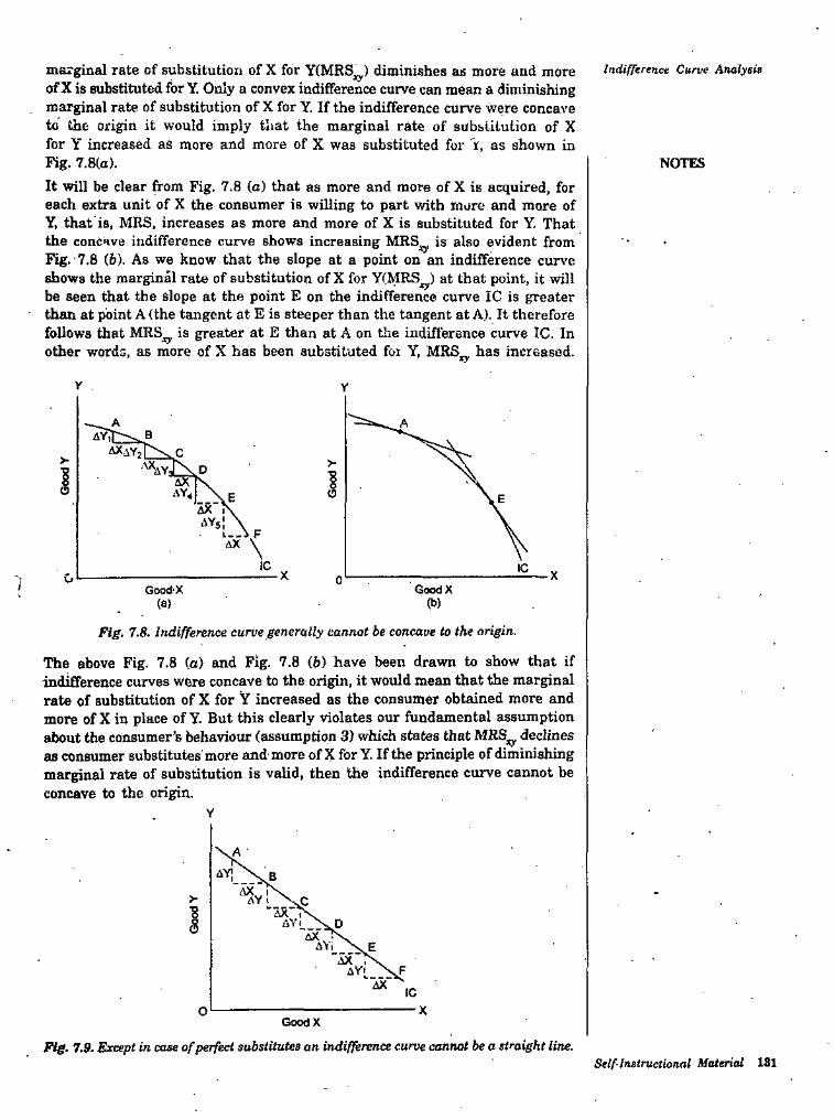
marginal rate of substitution of X for Y(MRS^) diminishes as more and more of X is substituted for Y. Only a convex indifference curve can mean a diminishing marginal rate of substitution of X for Y. If the indifference curve were concave to the origin it would imply that the marginal rate of substitution of X for Y increased as more and more of X was substituted for r, as shown in Fig. 7.8(a).It will be clear from Fig. 7.8 (o) that as more and more of X is acquired, for each extra unit of X the consumer is willing to part with more and more of Y, that'is, MRS, increases as more and more of X is substituted for Y. That the concave indifference curve shows increasing MRS,^ is also evident from Fig. 7.8 (6). As we know that the slope at a point on an indifference curve shows the marginal rate of substitution of X for Y(MRS^) at that point, it will be seen that the slope at the point E on the indifference curve IC is greater than at point A (the tangent at E is steeper than the tangent at A). It therefore follows that MRS_^ is greater at E than at A on the indiflerence curve IC. In other words, as more of X has been substituted foi Y, MRS^ has increased.
Indifference Curve Analysis
NOTES
Y
> >•
7 0 GoodXGood'X(b)(a)
Fig. 7.8. Indifference curve generally cannot be concave to the origin.
The above Fig. 7.8 (o) and Fig. 7.8 (6) have been drawn to show that if indifference curves were concave to the origin, it would mean that the marginal rate of substitution of X for Y increased as the consumer obtained more and more of X in place of Y. But this clearly violates our fundamental assumption about the consumer’s behaviour (assumption 3) which states that declines as consumer substitutes more and more of X for Y. If the principle of diminishing marginal rate of substitution is valid, then the indifference curve cannot be concave to the origin.
Y
>-•gs
oGoodX
Fig. 7.9. Except in case of perfect substitutes an indifference curve cannot be a straight line.Self-Instructional Material 131
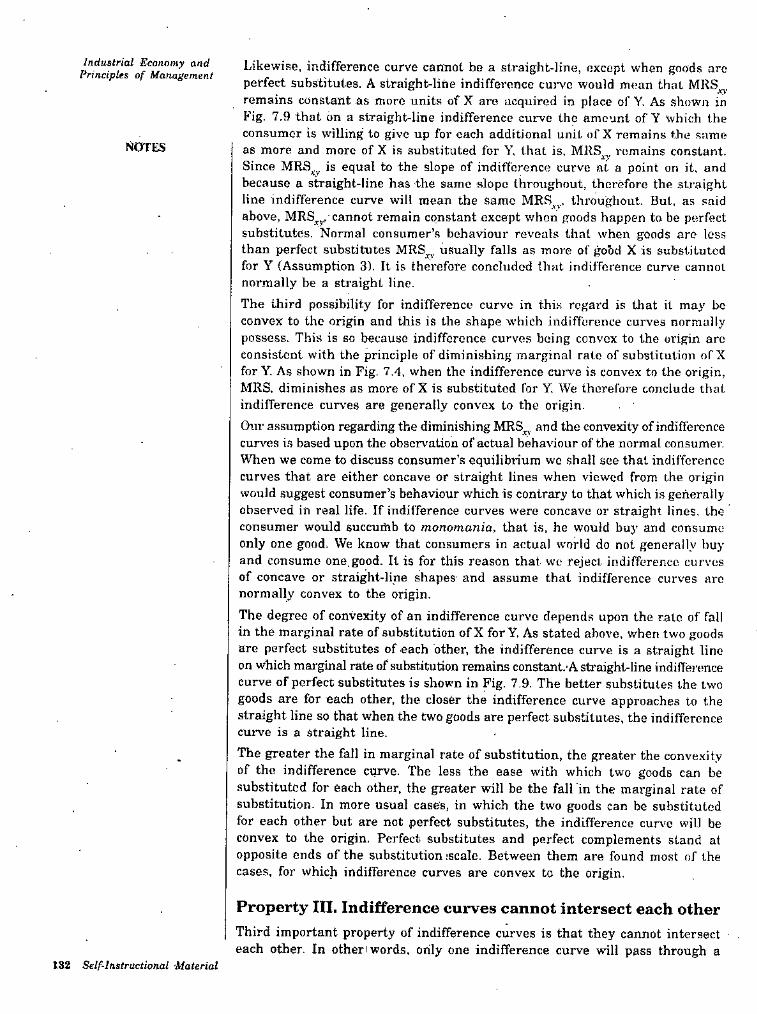
Induatrial Economy and Principles of Management Likewise, indifference curve cannot be a straight-line, except when goods arc
perfect substitutes. A straight-line indifference cui’ve would mean that MRS remains constant as more units of X are acquired in place of Y. As shown in P’ig. 7.9 that on a straight-line indifference curve the amount of Y which the con.5umcr is w’illing to give up for each additional unit of X remains the same as more and more of X is substituted for Y. that is, MRS^^, remains constant. Since MRS^^ is equal to the slope of indifference curve at a point on it. and because a straight-line has the same slope throughout, therefore the straight line indifference curve will mean the same MRS,,^,. throughout. But, as said above, MRS^^^ cannot remain constant except when goods happen to be perfect substitutes. Normal consumer’s behaviour reveals that when goads are less than perfect substitutes MRS.^^, usually falls as more of good X is substituted for Y (Assumption 3). It is therefore concluded that indifference curve cannot normally be a straight line.The third possibility for indifference curve in this regard is that it may be convex to the origin and this is the shape which indifference curves normally possess. This is so because indifference curves being convex to the origin are consistent with the principle of diminishing marginal rate of substitution of X for Y. As shown in Fig. 7.4, when the indifference curve is convex to the origin, MRS, diminishes as more of X is substituted for Y. We therefore conclude that indifference curves are generally convex to the origin.Our a.ssumption regarding the diminishing MRS_^. and the convexity of indifference curves is based upon the observation of actual behaviour of the normal consumer. When we come to discuss consumer’s equilibrium we shall see that indifference curves that are either concave or straight lines when viewed from the origin would suggest consumer’s behaviour which is contrary to that which is generally observed in real life. If indifference curves were concave or straight lines, the consumer would succuihb to monomania, that is, he would buy and consume only one good, We know that consumers in actual world do not generally buy and consume one.good. It is for this reason that we reject indifference curves of concave or straight-line shapes and assume that indifference curves are normally convex to the origin.
The degree of convexity of an indifference curve depends upon the rale of fall in the marginal rate of substitution of X for Y. As stated above, when two goods are perfect substitutes of each other, the indifference curve is a straight lino on which marginal rate of substitution remains constant.A straight-line indifference curve of perfect substitutes is shown in Fig. 7.9. The better substitutes the two goods are for each other, the closer the indifference curve approaches to the straight line so that when the two goods are perfect substitutes, the indifference curve is a straight line.The greater the fall in marginal rate of substitution, the greater the convexity of the indifference curve. The less the ease with which two goods can be substituted for each other, the greater will be the fall in the marginal rate of substitution- In more usual cases, in which the two goods can be substituted for each other but are not perfect substitutes, the indifference cur\'c will be convex to the origin. Perfect substitutes and perfect complements stand at opposite ends of the substitution iscale. Between them are found most of the cases, for which indifference curves are convex to the origin.
NOTES
Property III. Indifference curves cannot intersect each other
Third important property of indifference curves is that they cannot intersect each other. In otheriwords. only one indifference curve will pass through a
182 Self-Instructional Material
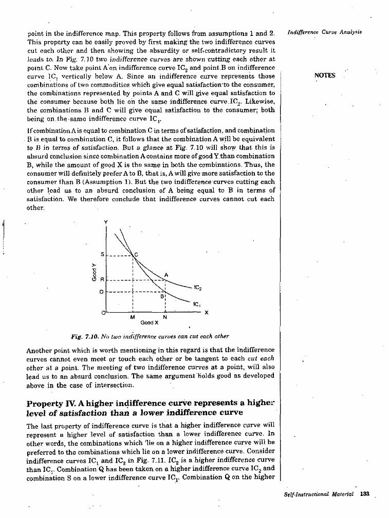
Indifference Curve Analysispoint in the indifference map. This property follows from assximptions 1 and 2. This property can be easily proved by first making the two indifference curves cut each other and then showing the absurdity or selfrcontradictory result it leads to. In Fig. 7.10 two indifference curves are shown cutting each other at point C. Now take point A on indifference curve ICj and point.B on indifference curve 1C, vertically below A. Since an indifference curve represents those combinations of two commodities which give equal satisfaction'to the consumer, the combinations represented by points A and C will give equal satisfaction to the consumer because both lie oh the same indifference curve.IC2. Likewise, the combinations B and C will give equal satisfaction to the consumer; both being on.the samc indifference curve IC,.
IfeombinationAis equal to combination C in terms of satisfaction, and combination B is equal to combination C. it follows that the combination A will be equivalent to B in terms of satisfaction. But a glance at Fig. 7.10 will show that this is absurd conclusion since combi nation A contains more ofgood Y.than combination B, while the amount of good X is the same in both the combinations. Thus, the consumer will definitely prefer A to B, that is, A will give more satisfactioh to the consumer than B (Assumption 1). But the two Indifference curves cutting each other lead us to an absurd conclusion of A being equal to B in terms of satisfaction. We therefore conclude that indifference curves cannot cut each other.
NOTES
s>-EO R
Q
XN
GoodX
Fig. 7.10. No two indifference curves can cut each other
Another point which is worth mentioning in this regard is that the indifference curves cannot even meet or touch each other or be tangent to each cut each other at a point. The meeting of two indifference curves at a point, will also lead us to an absurd conclusion. The same argument 'Holds good as developed above in the case of intersection.
Property IV. A higher indifference curve represents a higher level of satisfaction than a lower indifference curveThe last property of indifference curve is that a higher indifference curve will represent a higher level of satisfaction than a lower indifference curve. In other words, the combinations which ‘lie on a higher indifference curve will be preferred to the combinations which lie on a lower indifference curve. Consider indifference curves IC, and ICj in Fig. 7.11. ICg is a higher indifference curve than ICj. Combination Q has been taken on a higher indifference curve ICj and combination S on a lower indifference curve IC,. Combination Q on the higher
Self-Instructional Material 133
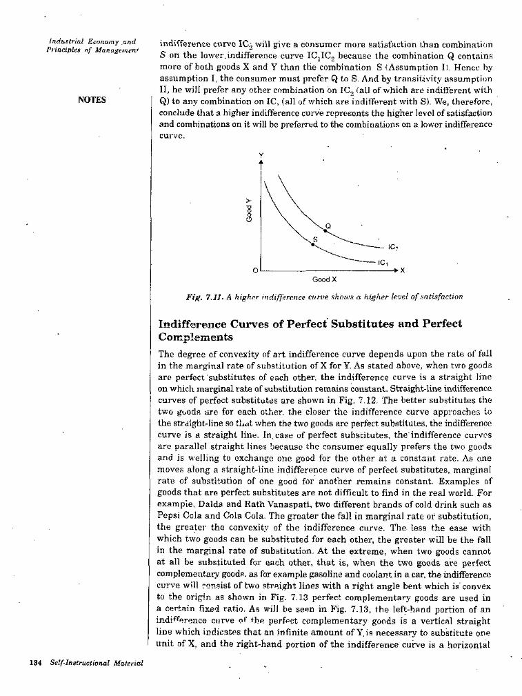
Industrial Economy and Principles of Management indifference curve ICj will give a consurncr more satisfaction than combination
S on the lower.indifference curve ICjICg because the combination Q contains more of both goods X and Y than the combination S (Assumption I). Hence by assumption I, the consumer must prefer Q to S. And by transitivity assumption II, he will prefer any other combination on IC2 (all of which are indifferent with Q) to any combination on IC, (all of which are indifferent with S). We, therefore, conclude that a higher indifference curve represents tlie higher level of satisfaction and combinations on it will be preferred to the combinations on a lower indifference curve.
NOTES
>-
o
o ♦ xGoodX
Fig. 7.11. A higher indifference curve shows a higher level of satisfaction
Indifference Curves of Perfect Substitutes and Perfect ComplementsThe degree of convexity of art indifference curve depends upon the rate of fall in the marginal rate of substitution of X for Y. As stated above, when two goods are perfect substitutes of each other, the indifference curve is a straight line on which marginal rate of substitution remains constant. Straight-line indifference curves of perfect substitutes are shown in Fig. 7.12. The better substitutes the two goods are for each other, the closer the indifference curve approaches to the straight-line so tliut when the two goods are perfect substitutes, the indifference curve is a straight line. In,case of perfect substitutes, the'indifference curves are parallel straight lines because the consumer equally prefers the two goods and is welling to exchange one good for the other at a constant rate. As one moves along a straight-line indifference curve of perfect substitutes, marginal rale of substitution of one good for another remains constant. Examples of goods that are perfect substitutes are not difficult to find in the real world. For example, Dalda and Rath Vanaspati, two different brands of cold drink such as Pepsi Cola and Cola Cola. The greater the fall in marginal rate or substitution, the greater the convexity of the indifference curve. The less the ease with which two goods can be substituted for each other, the greater will be the fall in the marginal rate of substitution. At the extreme, when two goods cannot at all be substituted for each other, that is, when the two goods are perfect complementary good.o. as for example gasoline and coolant.in a car, the indifference curve will consist of two straight lines with a right angle bent which is' convex to the origin as shown in Fig. 7.13 perfect complementary goods are used in a certain fixed ratio. As will he seen in Fig. 7.13, the left-hand portion of an indifference curve of the perfect complementary goods is a vertical straight line which indicates that an infinite amount of Y.is necessary to substitute one unit of X, and the right-hand portion of the indifference curve is a horizontal
134 Self Instructional Material
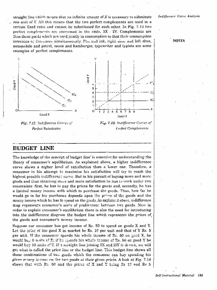
Indifference Curve AnalyxisStraight line '-vhi'‘h nr-'ans that an infinite amount of^ is necessary to substitute . one unit of K All this means that the two perfect complements are used in a
certain fixed ratio and cannot be substituted for each other. In Fig. 7.Id two perfect comp!'-n'.!'''.ls are consumed in, the ratio, 3X : 2Y. Complements are tl'.us those gocdii which are used jointly in consumption so that their consumption increases 0/ doCicasos simulUmeously. Pc-n and ink, rigiiL oliou aud left shoe, automobile and petrol, sauce and hamburger, typewriter and typists are some examples of perfect complements.
NOTES
>•D
> . IC-t■p
5O4
3 3iC2
1L'lOL X O 123456789
Good X Good X
Fig. 7.13. fnaifferinc!’. Curves offcrfect Complement.';
Fiff. 7J2 Indifferc.Hcc Cf.r>-s.; of Perfect Substitutes
BUDGET LINEThe knowledge of the concept of budget line’ is essentin I for understanding the theory of consumer’s equilibrium. As explained above, a higher indifference curve shows a Higher level of satisfaction than a lower one. Therefore, a consumer in his attempt to maximise his satisfaction will try to reach the highest possible indifference curve. But in his pursuit of buying more and more goods and liius oblainnig iriuie and more satisfaction he has to work under two constraints: first, he has to pay the prices for the goods and, secondly, he has a limited money income with which to purchase the goods. Thus, how far he would go in for his purchases depends upon the preea of the goods and the money income wluch he has to spend on the goods. As explained above, indifferonce map represents con.sumor’s scf'e of prefercnccf: betv.’een two goods. Now in order to explain consumer’s eauilibrium there is also the need for introducing into the indifference diagram the budget line which represents the prices of, the goods and consumer’s money income.Suppose our consumer has got income of Ks. 50 to spend on goods X and Y. Let the price of the good X in market be Rs. 10 per unit and that of Y Rs. 5 per unit. Jf the consumer spends his whole income of Rs. 50 on geed X, he would buy 5 u.'its of X; if ho eponds his v/holo income of E.s. 50 on good Y he would buy 10 units o^Y. If 1 straight line joining 5X and lOY ia di av-n, we will gei what is called the price line or the budget line. This budget line shows all those combinations of twu goods which the consunier can buy spending his given money ircomr on the two goods at fkeir given prices. A look at Fig. 7.14 shows that with Rc. 50 and tho prices cf X and Y being Rt 1? and Rs 5
Self-Instructional Material 135
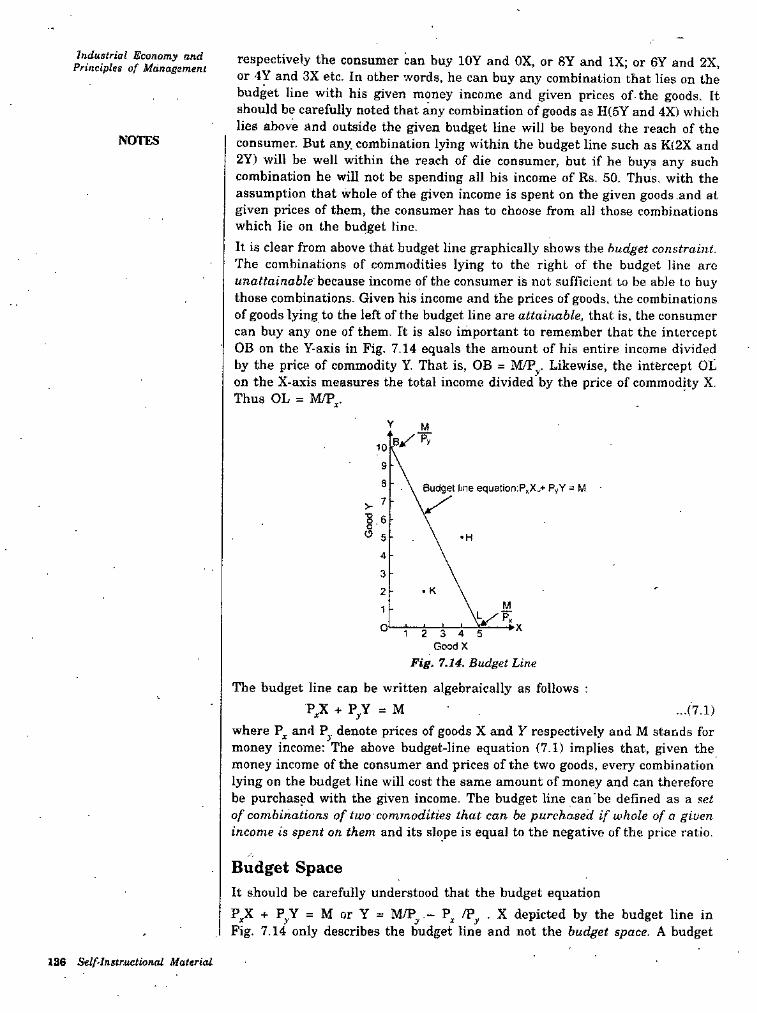
Industrial Economy and Principles of Mdnascment respectively the consumer can buy lOY and OX, or 8Y and XX; or 6Y and 2X,
or 4Y and 3X etc. In other words, he can buy any combination that lies on the budget line with his given money income and given prices of the goods. It should be carefully noted that any combination of goods as H(5Y and 4X) which lies above and outside the given budget line will be beyond the reach of the consumer. But any. combination lying within the budget line such as K{2X and 2Y) will be well within the reach of die consumer, but if he buys any such combination he will not be spending all his income of Rs. 50. Thus, with the assumption that whole of the given income is spent on the given goods .and at given prices of them, the consumer has to choose from all those combinations which lie on the budget line.It is clear from above that budget line graphically shows the budget constraint. The combinations of commodities lying to the right of the budget line are nna«amo6Ie'because income of the consumer is not sufficient to be able to buy those combinations. Given his income and the prices of goods, the combinations of goods lying to the left of the budget line are attainable, that is. the consumer can buy any one of them. It is also important to remember that the intercept OB on the Y-ajcis in Fig. 7.14 equals the amount of his entire income divided by the price of commodity Y. That is, OB = M/P^. Likewise, the intercept Ot on the X-axis measures the total income divided by the price of commodity X. Thus OL = M/P^.
NOTES
M
1098 Budget Ime equation;P,X,* PyY = M
V 7E 6O '« 5 •H
4
3. K2
M1
O ►X1 2 3 4 5GoodX
Fig. 7.14. Budget Line
The budget line can be written algebraically as follows :+ P/ = M
where P^ and P^. denote prices of goods X and Y respectively and M stands for money income: The above budget-line equation (7.1) implies that, given the money income of the consumer and prices of the two goods, every combination lying on the budget line will cost the same amount of money and can therefore be purchased with the given income. The budget line can'be defined as a set of combinations of two commodities that can be purchased if whole of a given income is spent on them and its slope is equal to the negative of the price ratio.
...(7.1)
Budget SpaceIt should be carefully understood that the budget equationP^X + P^Y = M or Y = M/P^ .- P^ /P, . X depicted by the budget line inPig- 7.14 only describes the budget line and not the budget space. A budget
136 Selflnstructional Material
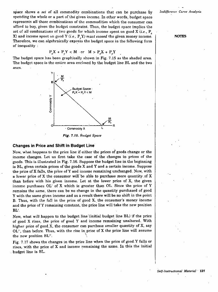
space shows a set of all commodity combinations that can be purchase by spending the whole or a part of the given income. In other words, budget space represents all those combinations of the commodities which the consumer can afford to buy, given the budget constraint. Thus, the budget space implies the set of all combinations of two goods for which income spent on good X (he.,X) and income spent on good Y (he., must exceed the given money income. Therefore, we can algebraically express the budget space in the following form of inequality :
Indifference Curve Analysis
NOTES
P_,X + P^Y < M or M > P_^X + P^YThe budget space has been graphically shown in Fig. 7.15 as the shaded area. The budget space is the entire area enclosed by the budget line BL and the two axes.
Y• M
B
Budget Space: P,X«-P,Y<M
VS'
eEo
M^ P.--------- Xo u• Coirmodity X
Fig. 7.15. Budget Space
Changes in Price and Shift in Budget LineNow, what happens to the price line if either the prices of' goods change or the income changes. Let us first take the case of the changes in prices of the goods. This is illustrated in Fig. 7.16. Suppose the budget line in the beginning is BL, given certain prices of the goods X and Y and a certain income. Suppose the price of X falls, the price of Y and income remaining unchanged. Now, with a lower price ofX the consumer will'be able to purchase more quantity of X than before with his given income. Let at the lower price of X, the given income purchases OL' of X which is greater than OL. Since the price of Y remains the same, there can be no change in the quantity purchased of good Y with the same given income and as a result there will be no shift in the point B. Thus, with the fall in the price of good X, the consumer’s money income and the price of Y remaining constant, the price line will take the new position BL'.Now, what will happen to the budget line (mitial budget line BL) if the price of good X rises, the price of good Y and income remaining unaltered. With higher price of good,X, the consumer can purchase smaller quantity of X, say OL", than before. Thus, with the rise in price of X the price line will assume the new position BL". \
Fig. 7.17 shows the changes in the price line when the price of good .Y falls or rises, with the price of X and income remaining the same. In this the initial
. budget line is BL.
Self-Instructional Material 137
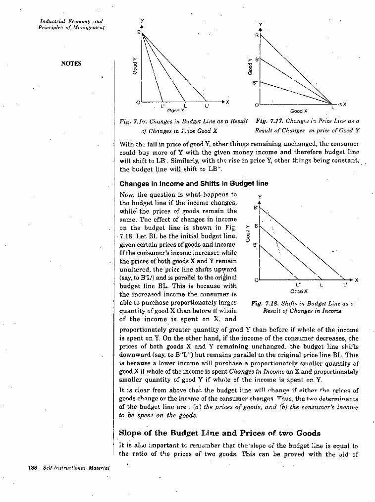
yIndustrial Economy and Principles of Management Y
♦ •SB’
V > aNOTES •g ■D
8oO o
B"
♦ XO -r:XoL. L" L’PqiiH y
FiE‘ Changes in Budget Line as u Result Fig. 7.17. Changes i-i Price Line, as a of Chav.ges in Price Good X
With the fall in price of good Y, other things remaining unchanged, the consumer could buy more of Y with the given money income and therefore budget line will shift to LB'. Similarly, with the rise in price Y, other things being constant, , the budget line will shift to LB”.
GoodX
Result of Changes m price of Good Y
Changes in Income and Shifts in Budget lineNow, the question is what happens to the budget line if the income changes, while' the prices of goods remain the same. The effect of changes in income on the budget line is shown in Fig.7.18. Let BL be the initial budget line, given certain prices of goods and income.If the consumer’s income increases while the prices of both goods X and Y remain unaltered, the price line shifts upward (say, to B'L') and is parallel to the original budget line BL. This is because with the increased income the consumer is able to purchase proportionately larger quantity of good X than before it whole of the income is spent on X, and proportionately greater quantity of good Y than before if whole of the income is spent on Y. On the other hand, if the income of the consumer decreases, the prices of both goods X and Y remaining.unchanged, the budget line shifts downward (say, to B"L'') but remains parallel to the original price line BL. This is because a lower income will purchase a proportionately smaller quantity of good X if whole of the income is spent Changes in Income on X and proportionately smaller quantity of good Y if whole of the income is spent on Y.It is clear from above, that the budget line will rhango if either fhe nrines of goods change or the income of the consumer changes 'I'hus, the two determinants of the budget line are : (a) the prices of goods, and (h) the consumer’s income to be spent on the goods.
Y
B'
.r B8o
B"
O XL" L L'
C:odX
Fig. 7.18. Bhifls in Budget Line as a Result of Changes in Income
Slope of the Budget Line and Prices of two GoodsIt is aLo important tc remember that the'slope of the budget Kne is equal to the ratio of the piices of two goods. This can be proved with the aid' of
138 Self-Instructional Material
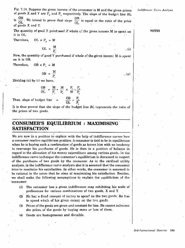
Fie. 7.14. Suppose the given income of the consumer is M and the given prices of goods X and Y are and respectively, The slope of the budget line BL. OB
hidiffercncv Ciirru Ann/ystK
to prove that slope is equal to the ratio of the priceof goods X and Y.IS
The quantity of good X purchased if whole of the given iiiC-ome M is spent on it is OL.Therefore,
NOTES
OL X 1>^ = M
MOL ...(«)
Now, the quantity of good Y purchased if whole of the .given income M is spent on it is OB,Therefore, OB X P^, = M
MOB ...Ui)PDividing (ii) by (f) we have.
OB M MOL P, P, ^ M " P^— -y
OB P.Thus, slope of budget line
It is thus proved that the slope of the budget line BL represents the ratio of the prices of two goods.
.....01. P,
CONSUMER'S EQUILIBRIUM : MAXIMISING SATISFACTIONWe are now in a position to explain with the help of indifference curves how a consumer reacho.s equilibrium position. A consumer is said to be in equilibrium when he is buying such a combination of goods as leaves him with no tendency to rearrange his purchases of goods. He is then in a position of balance in regard to the allocation of his money expenditure among various goods. In the indifference curve technique the consumer’s equilibrium is discussed in respect of the. purchases of two goods by the consumer. As in the cardinal utility analysis, in the indifference curve analysis also it is assumed that the consumer tries to maximize his satisfaction. In other words, the consumer is assumed to be rational in the sense that he aims at maximising his satisfaction. Besides, we shall make the following assumptions to explain t'ae equilibrium of the consumer:
The consumer has a given.indifference map exhibiting his scale of preferences for various combinations of two goods, X and Y.Ke has a fixed amount of mcney to spend on the two .goods. He has to spend whole of his given money on the tv-'c good®.Prices of the goods are given and constant for him. Ke cannot infiuunce the prices of the goods by buying mine or less of them.Goods are homogeneous and divisible.
(1)
(2)
(3)
(4)
Spif-Irtutruclioiial Material 139
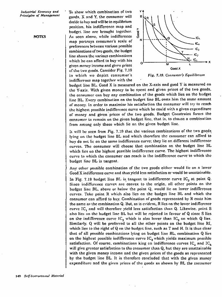
To show which combination of two goods, X and Y. the consumer will decide to buy and will be in equilibrium position, his indifference map and budget line are brought together.As seen above, while indifference map portrays consumer's scale of preferences between various i>ossible combinations of two goods, the budget line shows the various combinations which he can afford to buy with his given money income and given prices of the two goods. Consider Fig. 7.19 in which we depict consumer s indifference map together with the budget line BL. Good X is measured on the X-axis and good Y is measured on the Y-axis. With given money to be spent and given prices of the two goods, the consumer can buy any combination of the goods which lies on the budget line BL. Every combination on the budget line BL costs him the same amount of money, in order to maximise his satisfaction the consumer vrill try to reach the highest possible indifference cur\-c which he could with a given expenditure of money and given prices of the two goods. Budget Constraint forces the consumer to remain on the given budget line, that is. to chouse a combination from among only those which lie on the given budget line.
It will he seen from Fig. 7.19 lhai ihe various combinations of the two goods Iving on the budget line BL and which therefore the consumer can afford to buy do not lit on the same indifference curve; they lie on different indifference curves. The consumer will choose that combination on the budget lino BL which lies on the highest possible indifference curve. The highest indifference cur\’e to which the consumer can reach is the indifference cuiwe to which the budget line BL is tangent.
Any other possible combination of the two goods either would lie on a lower Good X indifference curve and thus yield less satisfaction or would be unattainable.In Fig. 7.19 budget line BL is tangent to indiffcronce cur\-e ICg at point Q. Since indifforcnce cun'cs are convex to the origin, all other points on the budget line BL. above or below the point Q. would lie on lower indifference curves. Take point R which also lies on the budget line BL and which the consumer can afford to buy. Combination of goods represented by R costs him the same as the combination Q. But, as is c\'ideni, R lies on the lower indilferonce curve IC, and will therefore xicld less satisfaction than Q. Likewise, point S also lies on the budget line BL but will be rejected in favour of Q since S lies on the indifference curve ICj which is also lower than IC3 on which Q lies. Similarly. Q will be preferred to all the other points on the budget line RI, which lies to the right of Q on the budget line, such as T and H. It is thus clear that of all possible combinations lying on budget line BL, combination Q lies on the highest possible indifrerence curve IC3 which yields maximum possible satisfaction. Of course, combinations king on indifference curves IC^ and IC^ will give greater satisfaction to the consumer than Q, but they are unattainable with the given money income and the given prices of the goods as represented by the budget line BL. If is therefore concluded that wnth the given money expenditure and the given prices of the goods as shown by BL the consumer
yIntiusirial Kconoiiiy end Prineiplex of Manegemenl B
>
NOTICSN
XO M LGoodX
Fif>. 7.19. Cons-uinrr',’1 Equilibrium
i<10 Srlf-ln’!l''urtif.t>ul Malftrial
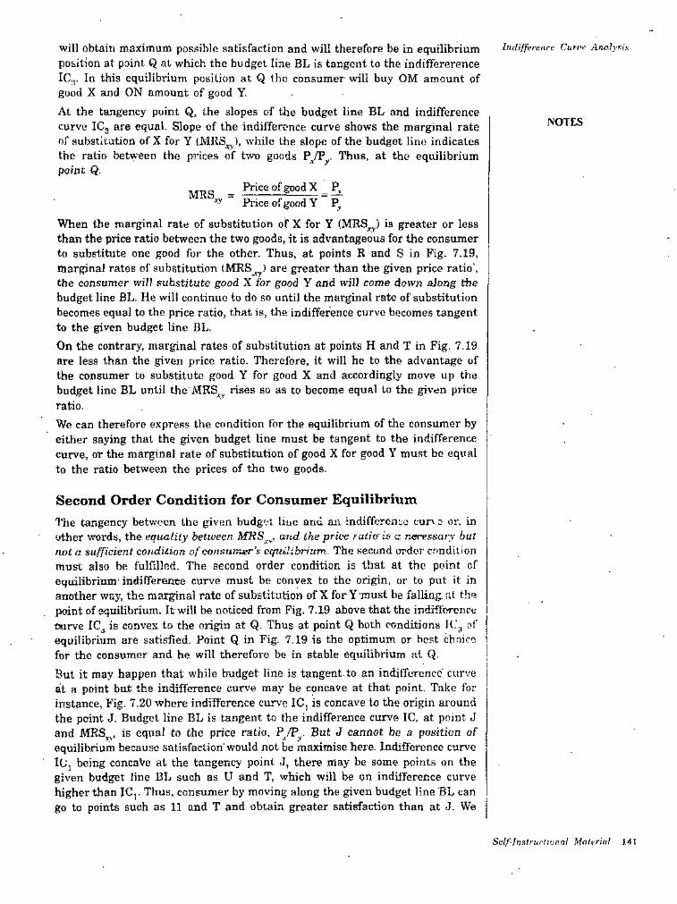
Inclif’ferenrc Cun'c Ano.ly^hwill obtain maximum possible satisfaction and will therefore be in equilibrium position at point Q at which the budget line BL is tangent to the indifFererence IC.j. In this equilibrium position at Q the consumer will buy OM amount of good X and ON amount of good Y.At the tangency point Q, the slopes of the budget line BL and indifference curve IC3 are equal. Slope of the indifference curve shows the marginal rate of substitution of X for Y while the slope of the budget lino indicatesthe ratio between the prices of two goods P/Py Thus, at the equilibrium point Q.
NOTES
^ Price of good X P,Price of good Y
When the marginal rate of substitution of X for Y (MRS^) is greater or less than the price ratio between the two goods, it is advantageous for the consumer to substitute one good for the other. Thus, at points R and S in Fig. 7.19, marginal rates of substitution (MRS are greater than the given price ratio', the consumer will substitute good X for good Y and will come down along the budget line BL. He will continue to do so until the marginal rate of substitution becomes equal to the price ratio, that is, the indifference curve becomes tangent to the given budget line BL.On the contrary, marginal rates of substitution at points H and T in Fig. 7.19 are less than the given price ratio. Therefore, it will he to the advantage of the consumer to substitute good Y for good X and accordingly move up the budget line BL until the MRS^,, rises so as to become equal to the given price ratio.We can therefore express the condition for the equilibrium of the consumer by either saying that the given budget line must be tangent to the indifference curve, or the marginal rate of substitution of good X for good Y must be equal to the ratio between the prices of the two goods.
Second Order Condition for Consumer EquilibriumThe tangency between the given budget line and an indifference cur\e or. in other words, the equality between and the price ratio is c necessary butnot a sufficient condUian of consurner's equilibrium. The second order condition must also be fulfillRci. The second order condition is that at the point of equilibrium-indifference curve must be convex to the origin, or to put it in another way, the marginal rate of substitution of X for Y must be falling, at the point of equilibrium. It will be noticed from Pig. 7.19 above that the indifftvronce curve ICj is convex to the origin at Q. Thus at point Q both conditions It.'., of equilibrium are satisfied- Point Q in Fig. 7.19 is the optimum or host choice l for the consumer and he will therefore be in stable equilibrium at Q. |Bui it may happen that while budget line is tangent to an indifference' curve at a point but the indifference curve may be concave at that point. Take for instance, Fig. 7.20 where indilference cur\’e ICj is concave to the origin around the point J. Budget line BL is tangent to the indifference curve IC, at point J and MRSj^, is equal to the price ratio. P^/P.^- But J cannot be a position of equilibrium because satisfaction'would not be maximise here. Indifference curve
■ iCj being concaVe at the tangency point J, there may be some points on the given budget line BL such as U and T, which will be on indilference curve higher than IC,. Thus, consumer by moving along the given budget line BL can go to points such as 11 and T and obtain greater satisfaction than at J. We
Sdf'-histrurlrunnl Meiii-riul 141
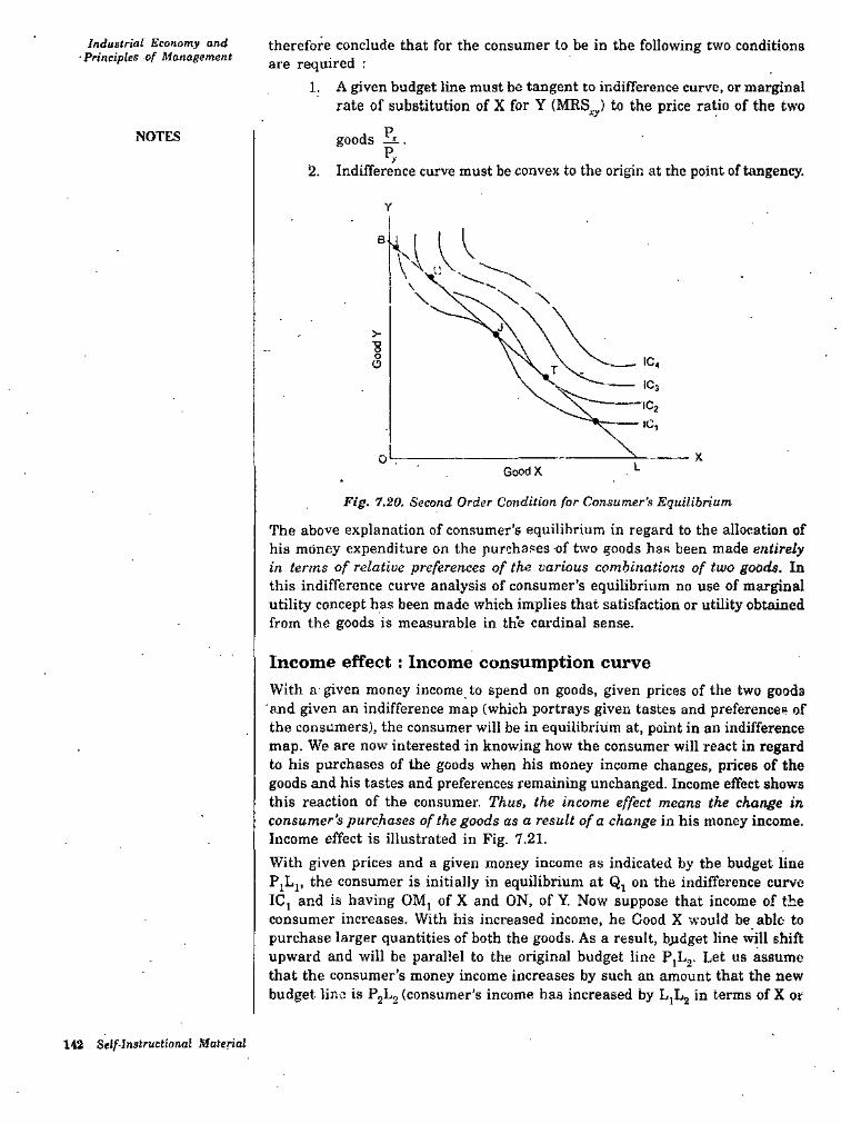
Industrial Economy and ■Principles of Management
therefore conclude that for the consumer to be in the following two conditions are required :
1, A given budget line must be tangent to indifference curve, or marginal rate of substitution of X for Y (MRS^^) to the price ratio of the two
pgoods —i..
P,2- Indifference curve must be convex to the origin at the point of tangency.
NOTES
B
>-
O
O LGoodX
Fig. 7.20. Second Order Condition for Consumer's Equilibrium
The above explanation of consumer’s equilibrium in regard to the allocation of his money expenditure on the purchases of two goods has been made entirely in terms of relative preferences of the various combinations of two goods. In this indifference curve analysis of consumer’s equilibrium no use of marginal utility concept has been made which implies that satisfaction or utility obtained from the goods is measurable in the cardinal sense.
Income effect : Income consumption curveWith a given money income to spend on goods, given prices of the two goods and given an indifference map (which portrays given tastes and preferences of the consumers), the consumer will be in equilibrium at, point in an indifference map. We are now interested in knowing how the consumer will react in regard to his purchases of the goods when his money income changes, prices of the goods and his tastes and preferences remaining unchanged. Income effect shows this reaction of the consumer. Thus, the income effect means the change in consumer’s purchases of the goods as a result of a change in his money income. Income effect is illustrated in Fig. 7.21.With given prices and a given money income as indicated by the budget line P^Lj, the consumer is initially in equilibrium at Qj on the indifference curve IC, and is having OM, of X and ON, of Y. Now suppose that income of the consumer increases. With his increased income, he Good X would be able to purchase larger quantities of both the goods. As a result, budget line will shift upward and will be parallel to the original budget line P]L2. Let us assume that the consumer’s money income increases by such an amount that the new budget lir.o is PjLj (consumer’s income has increased by LjLj in terms of X or
142 Seff-Inslruetional Moterioi
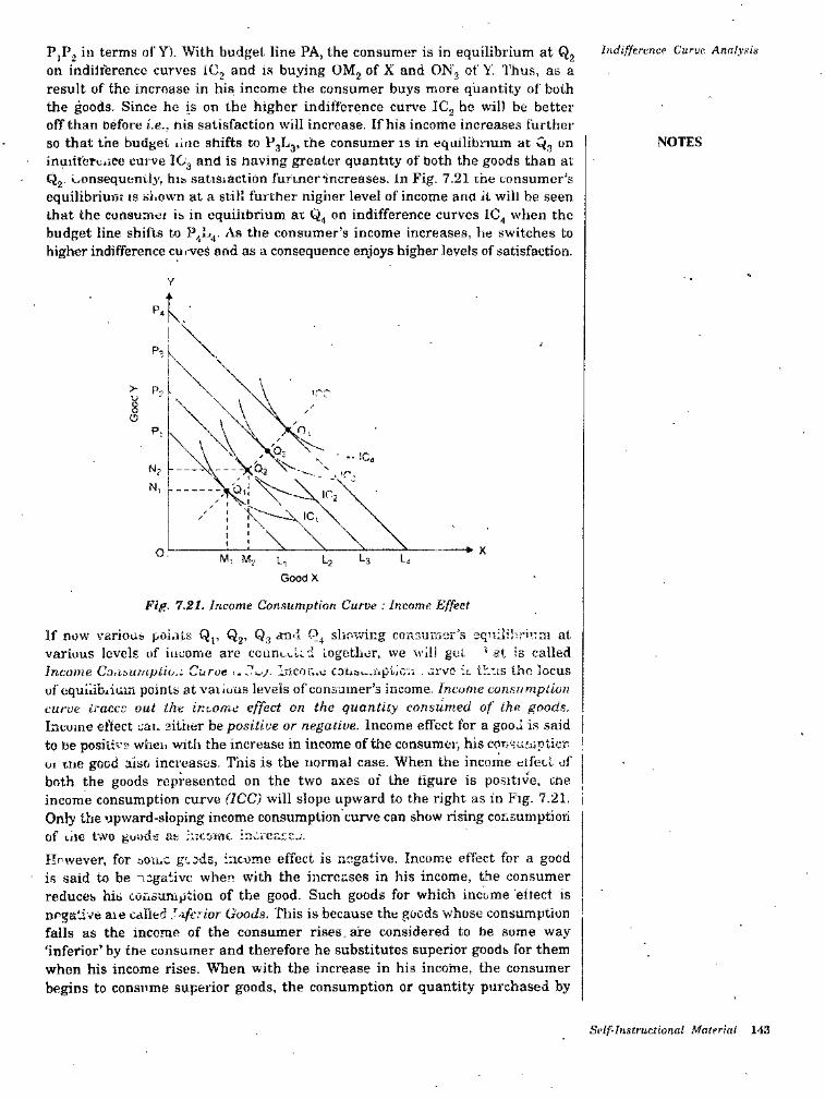
IndifftrcncP Curuf. AnnlyiiisPjP^ in terms ol' Y). With budget line PA, the consumer is in equilibrium at Q2 on indilierenco curves ICj and is buying OMj of X and ON, of’ Y. Thus, as a result of the increase in his income the consumer buys more quantity of both the goods. Since he is on the higher indifference curve JCj he will be better off than oefore i.e., nis satisfaction will increase. If hia income increases further so that the budget litic shifts to p3L3, the consumer is in equilibrium at Qg on inaitferciCe curve ICg and is having greater quantity of both the goods than at Qg. oonsequentiy, his satiSiaclion furincr increases. In Fig. 7.21 the consumer's equilibrium is siiown at a still further nigher level of income ana it will be seen that the conaurner is in equilibrium at on indifference curves IC,, when the budget line shifts to P,,^. As the consumer’s income increases, he switches to higher indifference cui-ves and as a consequence enjoys higher levels of satisfaction.
NOTES
Y
P4
P,
'iop.
Nj
N
-► XO L3 L.M-, M.,
Good X
Fif*. 7.21. Income Consumption Curve : Income Effect
If now various points Q,, Qj, Qg and slsov/ing consumer’s equilibrium at various levels of income are coiinL.\.Lcd logetLor, we will gut 'at is called Income Co.ibUinpUo.: Curve Incor-e couo.—r.pticr. . urvo ;l Ulus the locusof equiiibiiuin points at vaiiuus levels of consumer’s income. Income consiimpiion
iracce out the income effect on the quantity consumed of the goods. Income effect cat. sittier be positive or negative. Income effect for a good is said to be positive wheii with the increase in income of the consumer, his conMU'upticr. ! 01 me good also increases. This is the normal case. ’When the income eifect of both the goods represented on the two axes of the figure is positive, cne income consumption curve (ICC) will slope upward to the right as in Fig. 7.21. i Only the upward-sloping income consumption curve can show rising consumption of tiie two guilds as r.icorflt. incrcaECu.However, for ooiuc gcods, income effect is negative. Income effect for a good is said to be negative when with the increases in his income, the consumer reduces his coiisumption of the good. Such goods for which income efiect is negative aie called J-iferior Goods. This is because the goods whose consumption falls as the income of the consumer rises, are considered to be some way ‘inferior’ by ine consumer and therefore he substitutes superior goods for them when his income rises. When with the increase in his income, the consumer begins to consume superior goods, the consumption or quantity purchased by
curve
Self-Instructional Material 143
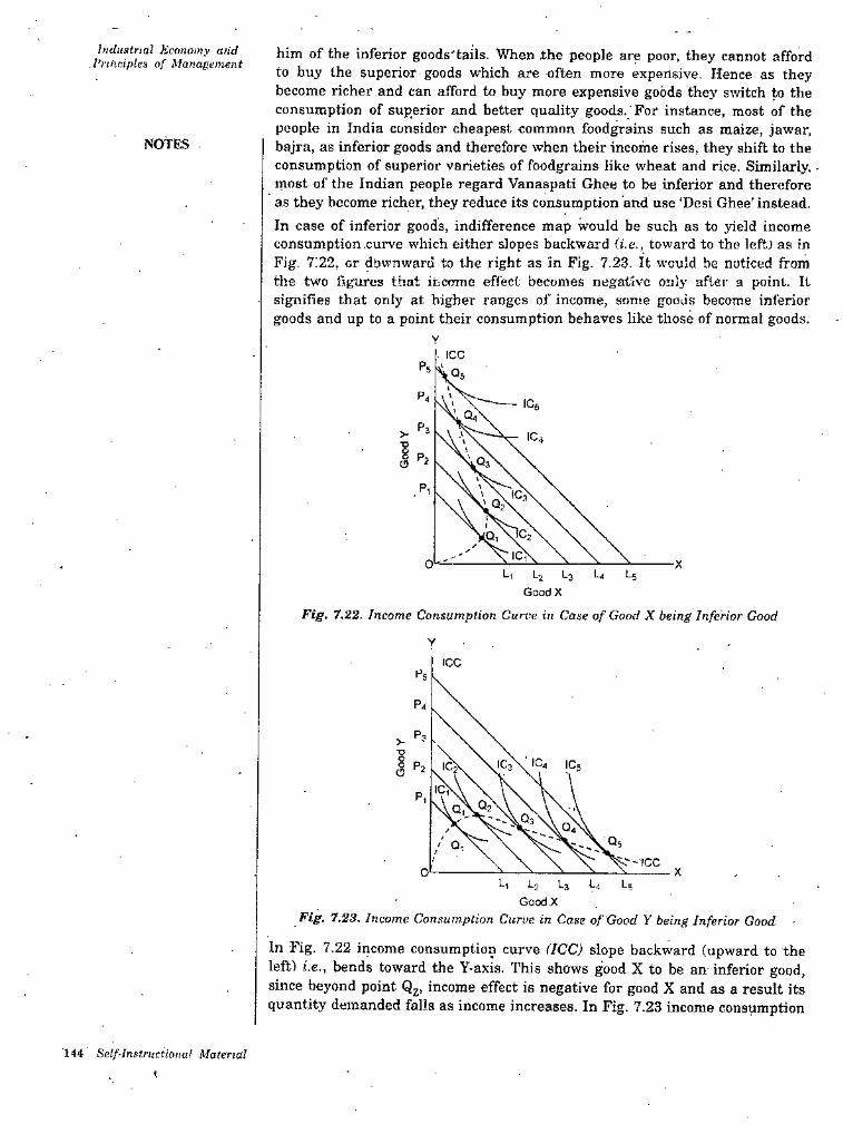
Industnal Jicfinoiny and I’rtnr.ipleH of Management him of the inferior goods'tails. When the people are poor, they cannot afford
to buy the superior goods which are often more expensive. Hence as they become richer and can afford to buy more expensive goods they switch to the consumption of superior and better quality goods. For instance, most of the people in India consider cheapest common foodgrains such as maize, jawar, bajra, as inferior goods and therefore when their income rises, they shift to the consumption of superior varieties of foodgrains like wheat and rice. Similarly. - most of the Indian people regard Vanaspati Ghee to be inferior and therefore as they become richer, they reduce its consumption and use ‘Desi Ghee’ instead. In case of inferior goods, indifference map would be such as to yield income consumption .curve which either slopes backward (i.c., toward to the left) as in Fig- 7:22, or downward to the right as in Fig. 7.23. It would be noticed from the two figures that it,come effect becomes negative only aftei- a point. It signifies that only at higher ranges of income, some goods become inferior goods and up to a point their consumption behaves like those of normal goods.
NOTES
ICCPs
P4
5 P, O ^1Pi
0 -XL, U t-51-2 L3
GoodX
Fig. 7.22. /ncome Consumption Cunn: in Case of Good X being Inferior Good
Y
ICCP5
P4
1 p op.
0L, L4^2
GoodX
Fig. 7.23. Income Consumption Curue in Case of Good Y being Inferior Good
In Fig. 7.22 income consumption curve (ICC) slope backward (upward to the left) i.e.. bends toward the Y-axis. This shows good X to be an inferior good, since beyond point Q2, income effect is negative for good X and as a result its quantity demanded falls as income increases. In Fig. 7.23 income consumption
L;
144 Self-lnstructiana! Material1
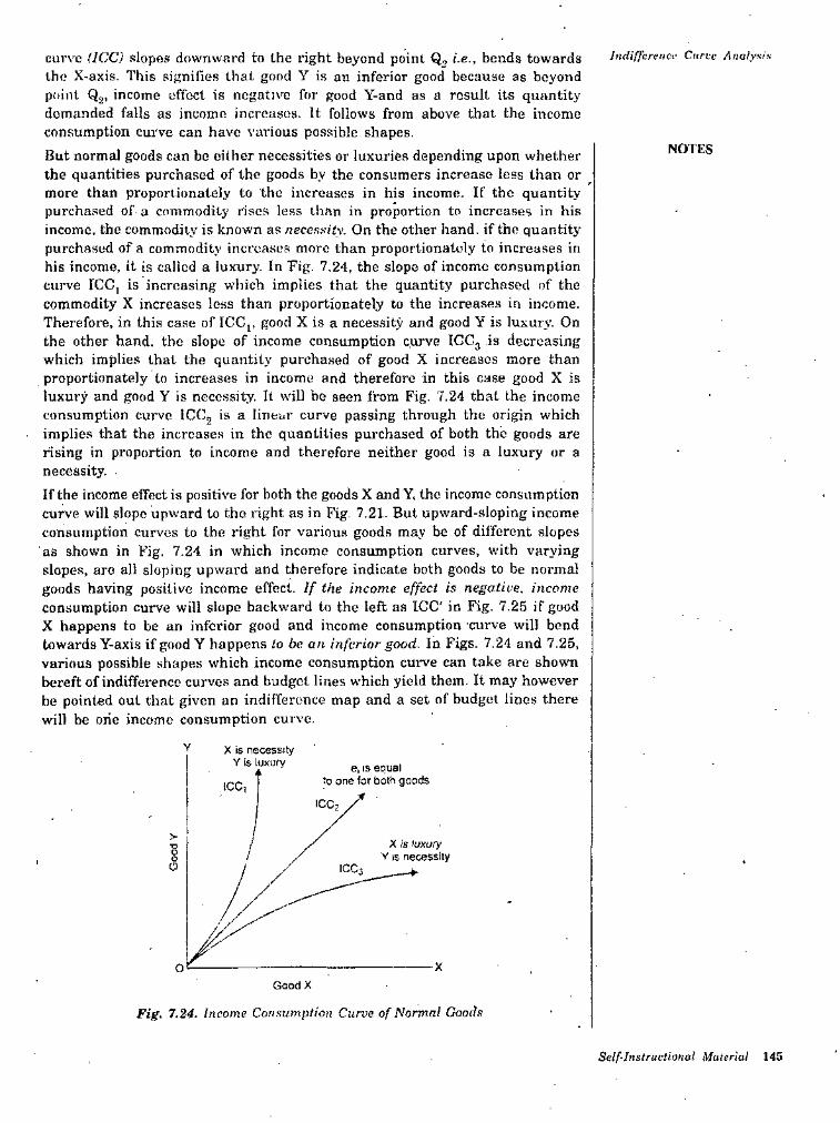
liiHiffcrenCf Curve Analysiscurve (ICC) slopes downward to the right beyond point Q, i.e., bends towards the X-axis. This signifies that good Y is an inferior good because as beyond point Qg, income effect is negative for good Y-and as a result its quantity demanded falls as income increases, it follows from above that the income consumption cui've can have various possible shapes.But normal goods can bo either necessities or luxuries depending upon whether the quantities purchased of the goods by the consumers increase less than or more than proportionately to the increases in his income. If the quantity purchased of a commodity rises less than in proportion to increases in his income, the commodity is known as necesmity. On the other hand, if the quantity purchased of a commodity increases more than proportionately to increases in his income, it is called a luxury. In Fig. 7.24, the slope of income consumption curve ICC, is increasing which implies that the quantity purchased of the commodity X increases less than proportionately to the increases in income. Therefore, in this case of ICC,, good X is a neces.sity and good ¥ is luxury. On the other hand, the slope of income consumption curve IGC3 is decreasing which implies that the quantity purchased of good X increases more than proportionately to increases in income and therefore in this case good X is luxury and good Y is necessity. It will be seen from Fig. 7.24 that the income consumption curve ICC, is a lint-ur curve passing through the origin which implies that the increases in the quantities purchased of both the goods are rising in proportion to income and therefore neither good is a luxury or a necessity.If the income effect is positive for both the goods X and Y, the income consumption curve will slope upward to the right as in Kg. 7.21. But upward-sloping income consumption curves to the right for variou.s goods may be of different slopes as shown in Fig. 7.24 in which income consumption curves, with varying slopes, arc all sloping upward and therefore indicate both goods to be normal goods having positive income effect. If the income effect is negative, income consumption curve will slope backward to the left os ICC' in Fig. 7.25 if good X happens to be an inferior good and income consumption curve will bond towards Y-axis if good Y happens lo be an inferior good. Id Figs. 7.24 and 7.25, various possible shapes which income consumption curve can take are shown bereft of indifference curves and budget lines which yield them. It may however be pointed out that given an indifference map and a set of budget lines there will be one income consumption curve.
NOTES
X is necessity Y is luxury e, IS epuai
to one for both goods
> X IS luxury Y IS necessity
■o
O
oGood X
Fig. 7.24. Income Consumption Curve of Normal Goods
Self-Instructional Malerial 145
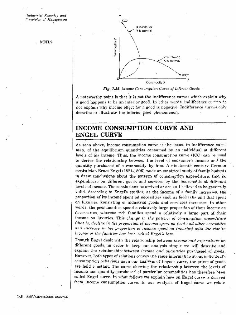
Iniiuslriat F.ciinohiy and Prinviples of MonaneniL’Hl ICC
\X is iifeiior Y is fiomial
. NOTES *ESoC „Y IS i.ifefio.',
X is notma!
ICC"O' X
Conimodity XFig. 7.25. Income Consumption Curve of Inferior Goods -
A noteworthy point is that it is not the indifference curves which explain why a good happens to be an inferior good. In other words, indifference cu-'C'-- do not explain why income effect for a good is negative. Indifference cur.-,!S erdy .describe or illustrate the inferior good phenomenon.
INCOME CONSUMPTION CURVE AND ENGEL CURVEAs seen above, income consumption curve is the locus, in indifference cur'-e map, of the equilibrium quantities consumed by an individual at different levels of bis income. Thus, the income consumption curve flCCl can be used to derive the relationship between the level of consumer’s income and the quantity purchased of a commodity by him. A nineteenth centurv German Statistician Emet Engel (1821-1896) made an empirical study of family budgets to draw conclusions about the pattern of consumption expenditure, that is. expenditure on different goods and services by the households at different- levels of income. The conslusions he arrived at are still boliovod to gepe"°l!y valid. According to Engel’s studies, as the income of a family incre'a?as, the proportion of its income spent on necessities such as food falls and that spent on luxuries fconsisting of industrial goods and services) increases. In other words, the poor families spend a relatively large proportion of their income on necessaries, whereas rich families spend a relatively a large part of their income on luxuries. This change in the pattern of consumption expenditure (that is, decline in the proportion of income spent on food and other necessities and increa.se in the proportion of income spent on luxuries) with the rise in income of the families has been called Engel’s law.Though Engel dealt with the relation,ship between income and expenditure on different goods, in order to keep our analysis simple m'g will describe and explain the relationship between income and quantities puri’hased of goods. However, both types of relations convey the same information about individual's consumption behaviour as in our analysis of Engel’s curve, the prices of goods are held constant. The curv’e showing the relationship between the levels of income and quantity purchased of particular commodities has therefore been called Engel cur%'e. In what follows we explain how an Engel curve is derived from income consumption curve. In our analysis of Engel curve we relate
146 Salf-InstructionaL Material
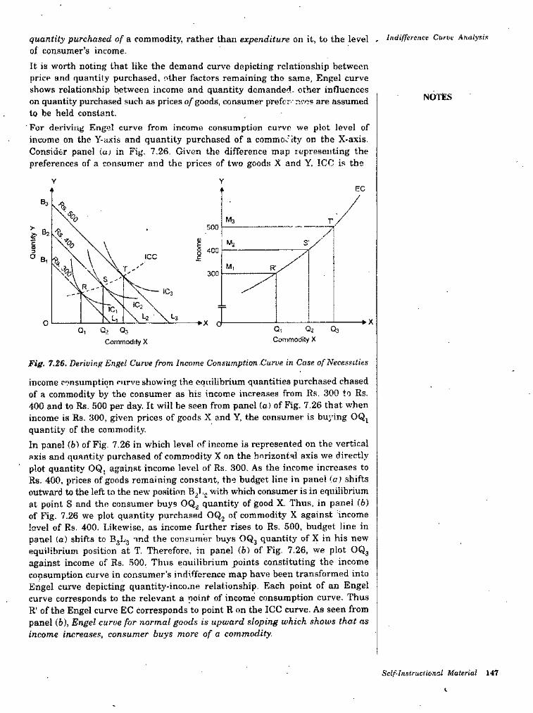
quantity purchased of a commodity, rather than expenditure on it, to the level - Indifference Curve Analyaix of consumer’s income.It is worth noting that like the demand curve depicting relationship between price and quantity purchased, other factors remaining the same, Engel curve shows relationship between income and quantity demanded- other influences on quantity purchased such as prices of goods, consumer prefer ' ncos are assumed to be held constant.For deriving Engel curve from income consumption curve we plot level of income on the Y-axis and quantity purchased of a commodity on the X-axis.Consider panel (uj in Fig. 7.26. Given the difference map representing the preferences of a consumer and the prices of two goods X and Y. ICC is the
NOTES
YEC
Bs
Ms500
* V M2o g 4003
° B, ICC £M, R'
300\R
O ♦x dQiQi Q2 Q3
Commodity X Commodity X
Fig. 7.26. Deriving Engel Curve from Income Consumption .Curve in Case of Necessities
income consumption curve showing the equilibrium quantities purchased chased of a commodity by the consumer as his income increases from Rs, 300 to Rs. 400 and to Rs. 500 per day. It will be seen from panel (c) of Fig. 7.26 that when income is Rs. 300, given prices of goods X and Y, the consumer is buying OQj quantity of the commodity.In panel (b) of Fig. 7.26 in which level of income is represented on the vertical axis and quantity purchased of commodity X on the horizontal axis we directly plot quantity OQ, against income level of Rs. 300. As the income increases to Rs. 400, prices of goods remaining constant, the budget line in panel (c) shifts outward to the left to the new position ^ vrith which consumer is in equOibrium at point S and the consumer buys OQ^ quantity of good X. Thus, in panel (b) of Fig. 7.26 we plot quantity purchased OQj of commodity X against income level of Rs. 400. Likewise, as income further rises to Rs. 500, budget line in panel (a) shifts to B3L3 and the consumer buys OQ3 quantity of X in his new equilibrium position at T. Therefore, in panel (b) of Fig. 7.26, we plot OQ3 against income of Rs. 500. Thus eauilibrium points constituting the income consumption curve in consumer’s indifference map have been transformed into Engel curve depicting quantity-income relationship. Each point of an Engel curve corresponds to the relevant a point of income consumption curve. Thus R’ of the Engel curve EC corresponds to point R on the ICC curve. As seen from panel (fej, Engel curve for normal goods is upward sloping which shows that as income increases, consumer buys more of a commodity.
Self-Instructional Material 147
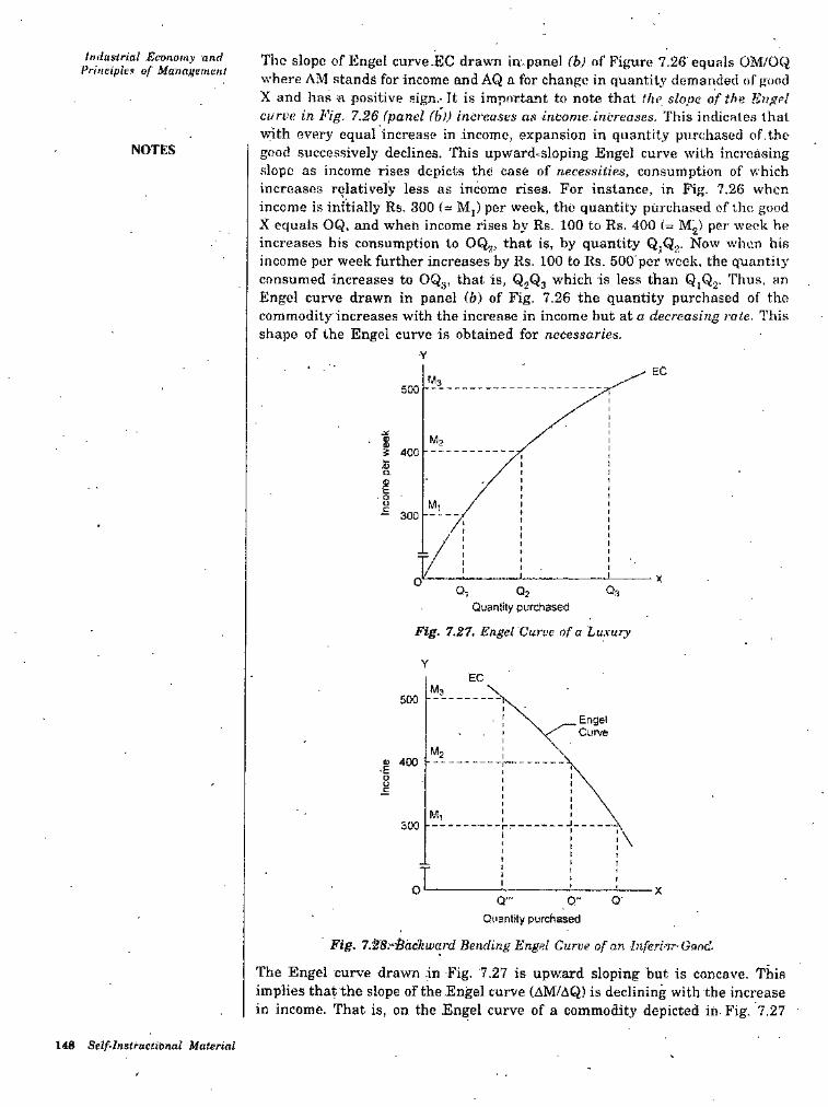
Imiiistrial Economy and Principle!) of Manat’emenI The slope of Engel curve.EC drawn in.panel (b) of Pigure 7.26 equals OM/OQ
where AM stands for income and AQ a for change in quantity' demanded of good X and has a positive sign.- It is important to note that the slope of the Engel curve, in Fig. 7.26 (panel (h)) increases as income.increases. This indicates that with every equal increase in income, expansion in quantity purchased of.the good successively declines. This upward-=sloping Engel curve with increasing slope as income rises depicts the case of necessities, consumption of which increases relatively less as income rises. For instance, in Pig. 7.26 when income is initially Rs. 300 (= Mj) per week, the quantity purchased of the good X equals OQ. and when income rises by Rs. 100 to Rs. 400 (= Mg) per week he increases his consumption to OQ,, that is, by quantity Q.Q^- when his income pur week further increases by Rs. 100 to Rs. 500'per week, the quantity consumed increases to OQ3, that is, Q2Q3 which is less than Q(Q2. Thus, an Engel curve drawn in panel (b) of Fig. 7.26 the quantity purchased of the coramodityincreases with the increase in income but at a decreasing rote. This shape of the Engel curve is obtained for necessaries.
NOTES
•YEC
M3500
• $3 400sQ.
Io- 300
XQ3Q- 02
Quantity purcOased
Fig. 7.27. Engel Curve of a Lu.xury
YEC
Ms500EngelCurve
M2o 400gc
M, \J300 r ^\
o Q„. 0" O'Quantity purchased
Fig. 7.28r'Bdekward Bending Engel Curve of an Inferhr Oand
The Engel curve drawn in Fig. 7.27 is upw:ard sloping but is concave. This implies that the slope of the Engel curve (AMMQ) is declining with the increase in income. That is, on the ,Engel curve of a commodity depicted in Fig. 7,27
148 Self-Instructional Material
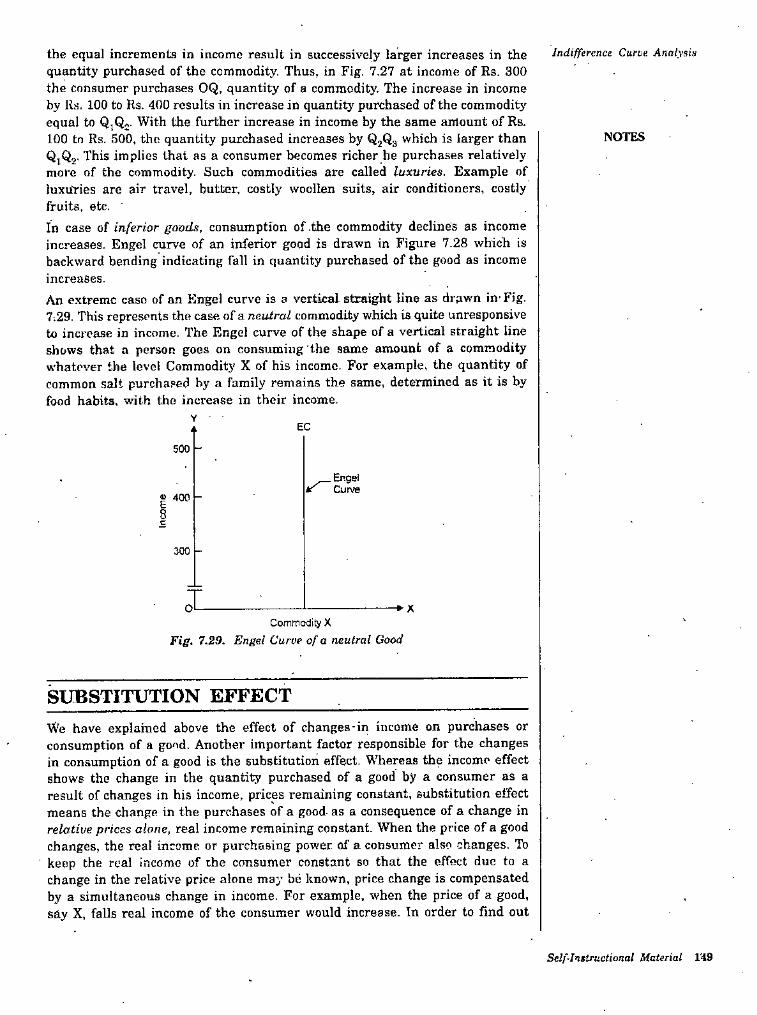
Indifference Curve Analysisthe equal increments in income result in successively larger increases in the quantity purchased of the commodity. Thus, in Fig. 7.27 at income of Rs. 300 the consumer purchases OQ, quantity of a commodity. The increase in income by Rs. 100 to Rs. 400 results in increase in quantity purchased of the commodity equal to QjQj- With the further increase in income by the same amount of Rs. 100 to Rs. 500, the quantity purchased increases by Q2Q3 which is larger than QjQ2. This implies that as a consumer becomes richer he purchases relatively more of the commodity. Such commodities are called luxuries. Example of luxuries are air travel, butter, costly woollen suits, air conditioners, costly fruits, etc.In case of inferior goods, consumption of .the commodity declines as income increases. Engel curve of an inferior good is drawn in Figure 7.28 which is backward bending indicating fall in quantity purchased of the good as income increases.An extreme cast) of an Engel curve is a vertical straight line as drawn in’Fig. 7;29. This represents the case of a neutral commodity which is quite unresponsive to increase in income. The Engel curve of the shape of a vertical straight line shows that a person goes on consuming the same amount of a commodity whatever the level Commodity X of his income. For example, the quantity of common salt purchased by a family remains the same, determined as it is by food habits, with the increase in their income.
NOTES
EC
500
Enge! » Curve
I 4008c
300
oCommodity X
Fig. 7.29. Engel Curve of a neutral Good
SUBSTITUTION EFFECTWe have explained above the effect of changes-in income on purchases or consumption of a good. Another important factor responsible for the changes in consumption of a good is the substitution effect. Whereas the income effect shows the change in the quantity purchased of a good by a consumer as a result of changes in his income, prices remaining constant, substitution effect means the change in the purchases of a good- as a consequence of a change in relative prices alone, real income remaining constant. When the price of a good changes, the real income or purchasing power of a consumer also changes, lb keep the real income of the consumer constant sti that the effect due to a change in the relative price alone may be known, price change is compensated by a simultaneous change in income. For example, when the price of a good, say X, falls real income of the consumer would increase. In order to find out
Self-Instructional Material I'iS
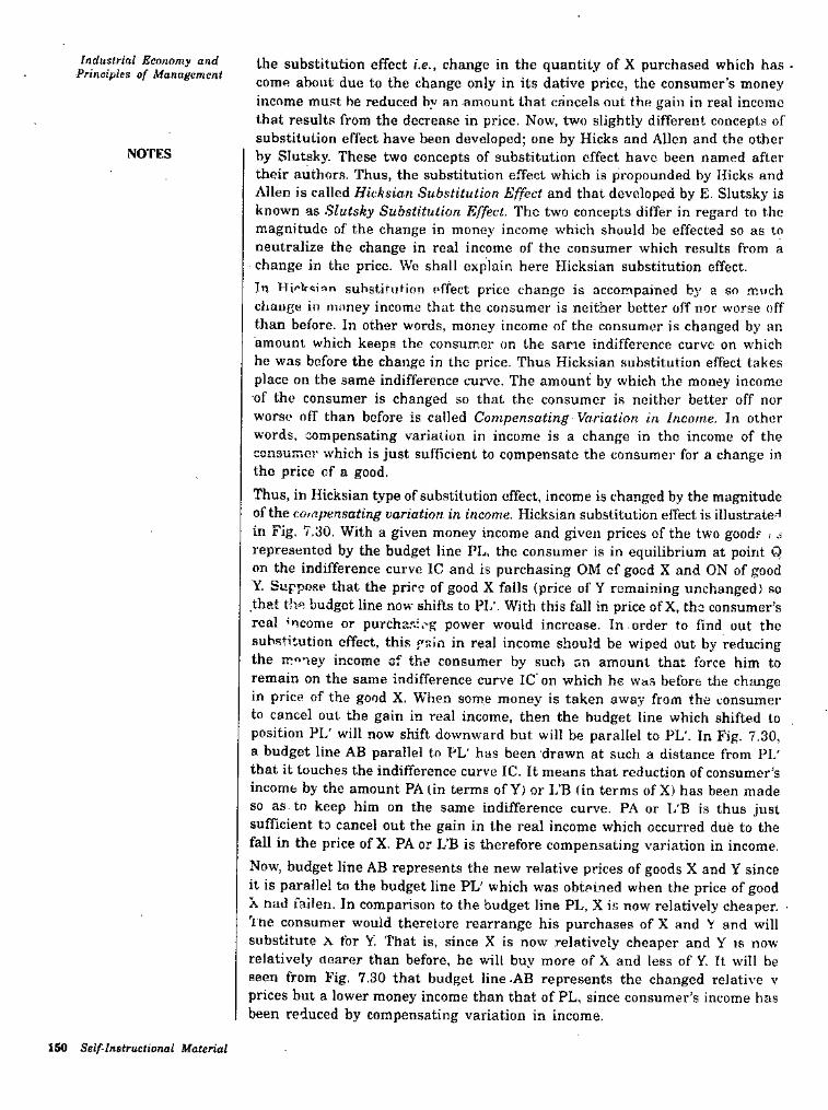
Industrial Ecnnomy and Principles of Management the substitution effect i.e., change in the quantity of X purchased which has •
come about due to the change only in its dative price, the consumer’s money income must he reduced by an amount that cancels out the gain in real income that results from the decrease in price. Now, two slightly different concepts of substitution effect have been developed; one by Hicks and Alien and the other by Slutsky. These two concepts of substitution effect have been named after their authors. Thus, the substitution effect which is propounded by Hicks and Allen is called Hicksian Substitution Effect and that developed by E. Slutsky is known as Slutsky Substitution Effect. The two concepts differ in regard to the magnitude of the change in money income which should be effected so as to neutralize the change in real income of the consumer which results from a change in the price. Wo shall explain here Hicksian substitution effect.In substitut-ion effect price change is accompained by a so muchchange in money income that the consumer is neither better off nor worse off than before. In other words, money income of the consumer is changed by an amount which keeps the consumer on the same indifference curve on which he was before the change in the price. Thus Hicksian substitution effect takes place on the same indifference curve. The amount by which the money income of the consumer is changed so that the consumer is neither better off nor worse off than before is called Compensating Variation in Income. In other words, compensating variation in income is a change in the income of the consumer which is just sufficient to compensate the consumer for a change in the price of a good.Thus, in Hicksian type of substitution effect, income is changed by the magnitude of the compensating variation in income. Hicksian substitution effect is illustrate^ in Fig, 7,30. With a given money income and given prices of the two goods represented by the budget line PL, the consumer is in equilibrium at point O on the indifference curve IC and is purchasing OM cf good X and ON of good Y. Suppose that the price of good X fails (price of Y remaining unchanged) so that t'w budget line now shifts to PL’. With this fall in price of X. the consumer’s real 'ncome or purcha-'-i.-g power would increase. In order to find out the substitution effect, this gsin in real income should be wiped out by reducing the m^ney income of the consumer by such an amount that force him to remain on the same indifference curve IC on which he was before the chjuige in price of the good X. When some money is taken away from the consumer to cancel out the gain in real income, then the budget line which shifted to position PL' will now shift downward but will be parallel to PL'. In Fig. 7.30, a budget line AB parallel to PL' has been drawn at such a distance from PL' that it touches the indifference curve IC. It means that reduction of consumer’s income by the amount PA (in terms ofY) or L'B (in terms ofX) has been made so as. to keep him on the same indifference curve. PA or L'B is thus just sufficient to cancel out the gain in the real income which occurred due to the fall in the price of X. PA or L’B is therefore compensating variation in income.Now, budget line AB represents the new relative prices of goods X and Y since it is parallel to the budget line PL' which was obtained when the price of good A nad faiieri. In comparison to the budget line PL, X is now relatively cheaper. • I ne consumer would thereiore rearrange his purchases of X and V and will substitute X for Y. That is, since X is now relatively cheaper and Y is now relatively aoarer than before, he will buy more of X and less of Y. It will be seen from Fig. 7.30 that budget )ine-AB represents the changed relative v prices but a lower money income than that of PL, since consumer’s income has been reduced by compensating variation in income.
NOTES
i .-i
150 Self-Instructional Material
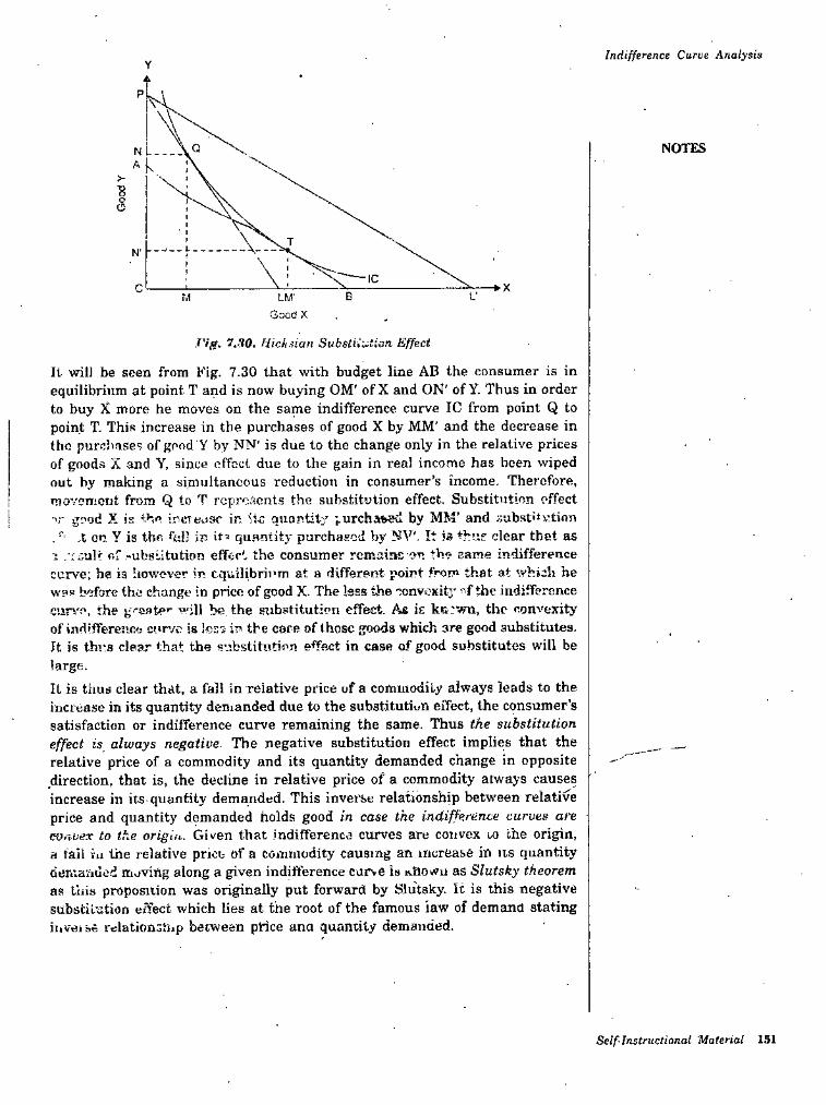
Indifference Curue AnalysisY
P
NOTESNA
>oO
N'
B 1'vl LM'GrjoO X
I'ig. 7.S0. Hicksian Subsiil-.^tian. Effect
II wilJ be seen from Kig. 7.30 that with budget line AB the consumer is in equilibrium at point T and is now buying OM' of X and ON' of Y. Thus in order to buy X more he moves on the same indifference curve IC from point Q to point T. This increase in the purchases of good X by MM' and the decrease in tho purchases of good Y by NN' is due to the change only in the relative prices of goods X and Y, since effect due to the gain in real income has been wiped out by making a simultanoous reduction in consumer’s income. Therefore, movement from Q to T represents the substitution effect. Substitution effect '>;• good X is tho ircreosc in iti quantity purchased by MM’ and sabst'‘v.tion , ,t on Y is tho <'e!’ in it’ quantity purchased by NV'. It is »hus dear tbet as 1 .'iiiult of -ubstitution effect the consumer remains on the came indifference curve: he is however in tquilibrii’m at a different point from that at which he w?R before tho change in price of good X. The less the convexit;- ^f the indifference cvirv'e, the g-sate’- will be the substitution effect. As is kc:wn, the convexity of ind'fferejic.'j ct»r/e is Icno in the care of those goods which are good substitutes. It is thi's clear that the substitution effect in case of good substitutes will be large.IL is tiius clear that, a fall in relative price of a commodily always leads to the increase in its quantity demanded due to the substitutiun effect, the consumer’s satisfaction or indifference curve remaining the same. Thus the substitution effect is always negative. The negative substitution effect implies that the relative price of a commodity and its quantity demanded change in opposite direction, that is, the decline in relative price of a commodity always causes increase in ies quantity demanded. This invei'Se relationship between relative price and quantity demanded holds good in case the indifference curves are convex to the origin. Given that .indifference curves are convex to che origin, a fail ill the relative price of a commodity causing an increase in its quantity demaiiucd moving along a given indifference carve is t^Bown as Slutsky theorem as this proposition was originally put forward by Slutsky. It is this negative substitution effect which lies at tne root of the famous law of demand stating iiiveibc relationship between price ana quantity demanded.
Self-Instructional Materia! 151
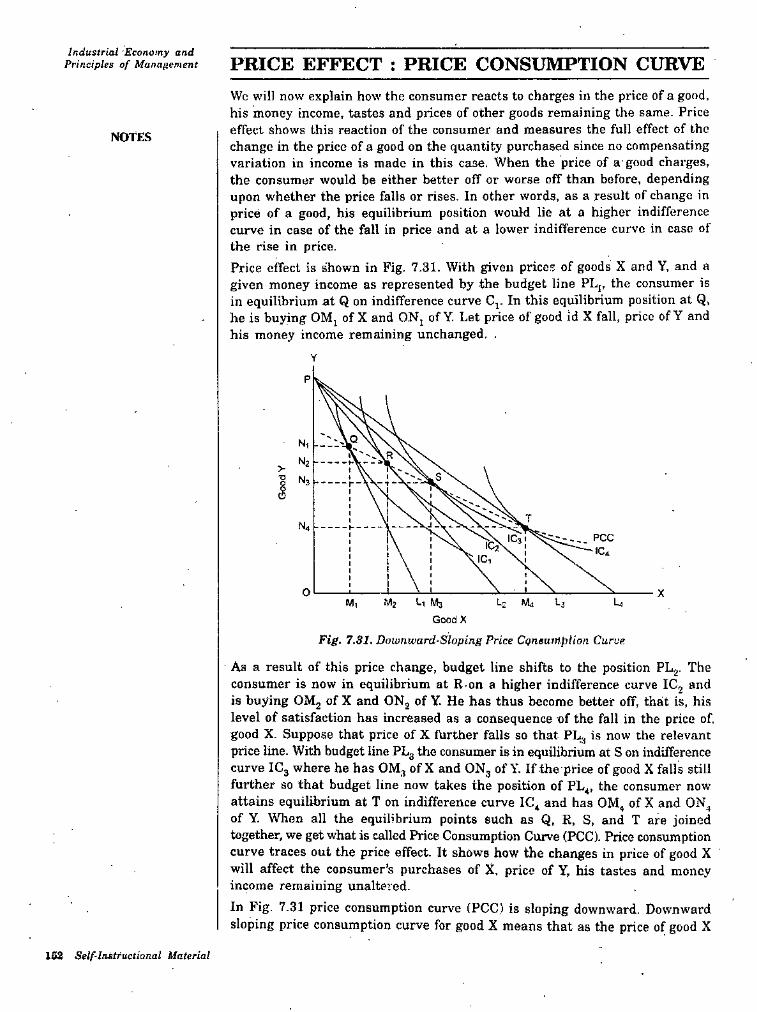
Industrial Economy and Principles of Mana/iement PRICE EFFECT : PRICE CONSUMPTION CURVE
Wc will now explain how the consumer reacts to charges in the price of a good, his money income, tastes and prices of other goods remaining the same. Price effect shows this reaction of the consumer and measures the full effect of the change in the price of a good on the quantity purchased since no compensating variation in income is made in this case. When the price of a good charges, the consumer would be either better off or worse off than before, depending upon whether the price falls or rises. In other words, as a result of change in price of a good, his equilibrium position would lie at a higher indifference curve in case of the fall in price and at a lower indifference curve in case of the rise in price.Price effect is shown in Fig. 7.31. With given prices of goods X and Y, and a given money income as represented by the budget line PL,, the consumer is in equilibrium at Q on indifference curve Cj. In this equilibrium position at Q, he is buying OM, of X and ON, of Y, Let price of good id X fall, price ofY and his money income remaining unchanged, .
NOTES
P
N,
>? Ns
N4
OMl Mj ti Mj t-j Li
Good XFig. 7.31. Downward-Sloping Price CgneutHplioii Cum
As a result of this price change, budget line shifts to the position PL2. The consumer is now in equilibrium at R. on a higher indifference curve ICj and is buying OMj of X and ONj of Y. He has thus become better off, that is, his level of satisfaction has increased as a consequence of the fall in the price of, good X. Suppose that price of X further falls so that PL., is now the relevant price line. With budget line PLg the consumer is in equUibrium at S on indifference curve IC3 where he has OM3 of X and ON3 of Y. If the price of good X falls still further so that budget line now takes the position of PL^, the consumer now attains equilibrium at T on indifference curve IC* and has OM, of X and ON_, of Y. When all the equilibrium points such as Q, R, S, and T are joined together, we get what is called Price Consumption Curve (PCC). Price consumption curve traces out the price effect. It shows how the changes in price of good X will affect the consumer’s purchases of X, price of Y, his tastes and money income remaining unaltered.In Fig. 7.31 price consumption curve (PCC) is sloping downward. Downward sloping price consumption curve for good X means that as the price of good X
152 Self-Instructional Material
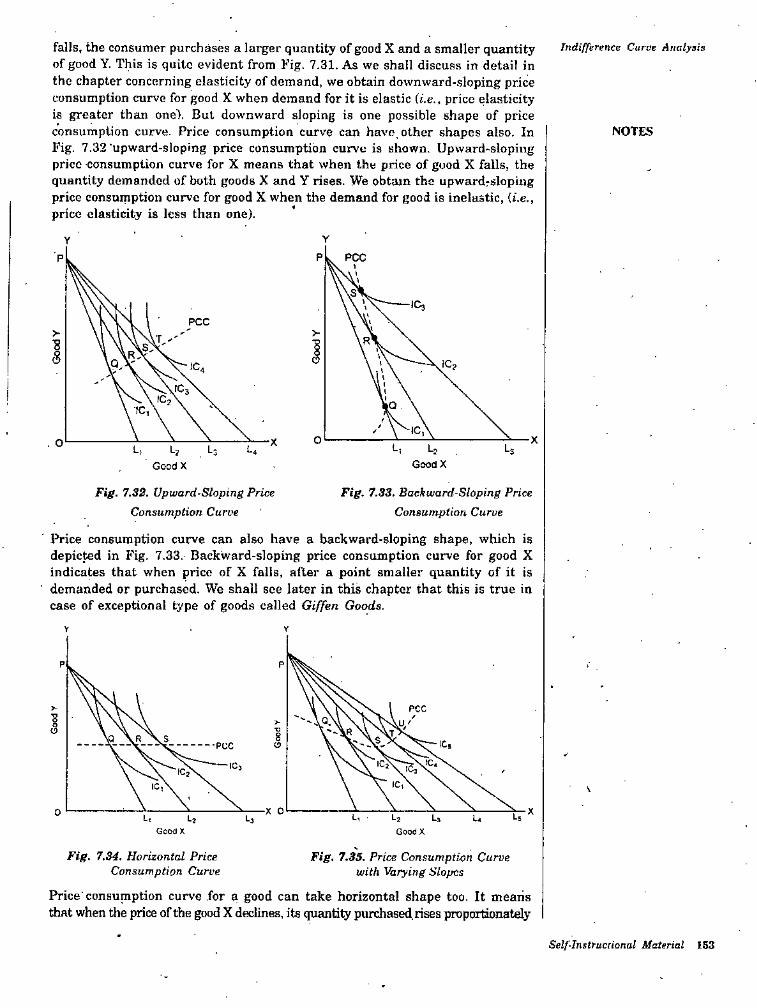
falls, the consumer purchases a larger quantity of good X and a smaller quantity of good Y. This is quite evident from Fig. 7.31. As we shall discuss in detail in the chapter concerning elasticity of demand, we obtain downward-sloping price consumption curve for good X when demand for it is elastic (i.e., price elasticity is greater than one). But downward sloping is one possible shape of price consumption curve. Price consumption curve can have, other shapes also. In Fig. 7.32'upward-sloping price consumption curve is shown. Upward-sloping price consumption curve for X means that when the price of good X falls, the quantity demanded of both goods X and Y rises. We obtain the upwardrsloping price consumption curve for good X when the demand for good is inelastic, (t.e., price elasticity is less than one).
Indifference Curve Analysis
NOTES
PP
> >■gs
0. o Lt 1-2Good X
LlL, Lj La L4GoodX
Fig. 7.32. Upward-Sloping Price Consumption Curve
Price consumption curve can also have a backward-sloping shape, which is depicted in Fig. 7.33. Backward-sloping price consumption curve for good X indicates that when price of X falls, after a point smaller quantity of it is
■ demanded or purchased. We shall see later in this chapter that this is true in case of exceptional type of goods called Giffen Goods.
Fig. 7.33. Backward-Sloping Price Consumption Curue
Y
p p
>->5 1o
-X 00 LsL, LjL, Lj U.Good X Gooax
Fig. 7.35. Price Consumption Curve with Varying Slopes
Price'consuniption curve for a good can take horizontal shape too. It meaiis that when the price of the good X declines, its quantity purchased, rises proportionately
Fig. 7.34. Horizontal Price Consumption Curve
Self-Instructional Material 153
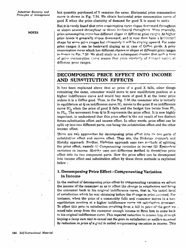
Industrial Economy and Principles of h’anagement
but quantity purchased.of Y remains the same. Horizontal price consumption curve is shown in Fig. 7.34. We obtain horizontal price consumption curve of good X when the price elasticity of demand for good X is equal to unitv.But it is rarely found that price consumption n.irve «lopee downward throughout or slopes upward throughout or alone= herlrvf/’rd throyghent Wnfo ce^prally, price consumption ciTiwe ha? different slope® ft different price ranges. At higher price levels it gonerally slopes downward, and it may then have a h^rizcTit?! shape for some prig's ranges but uitimately’t will be slop’pg upwa’-d. For some price ranges it can be backward sloping as in case of goods. A priceconsumption curve which has different shaoes or slope? at different price ranges ia flrowo in Pi|T. 7,,35 We shall study in a subsequent chanter that such a tvno of pri^'c consumption curve means that price elasticity of d-'roard vuric:; at different pnee ranges.
NOTES
DECOMPOSING PRICE EFFECT INTO INCOME AND SUBSTITUTION EFFECTSIt has been explained above that as price of a good X falls, other things remaining the same, consumer would move to new equilibrium position at a higher indifference curve and would buy more of good X at the lower price unless it is a Giffen good. Thus, in the Fig. 7.3fi the consumer who is initially in equilibrium at Q on indifference curve IC, moves to the point R on indifference curve ICj when the price of good X falls and the budget line twists from PLj to PLj. The movement from Q to R represents the price effect. It is now highly important, to understand that this price effect is the net result of two distinct forces-substitution effect and income effect. In other words, price effect can be split up into two different parts, one being the substitution effect and the other income effect.Tbf”'e are two approaches for decomposing price into ffe two parts nfsubstitution effect end income effect. They §fe, the Hicksian n^proarh and Slutsky approach. Further, Hick?ian approach uses two ir''*'hods of splitting the price effect, namely (i) Compensating variation in inomP. UV Kquivahrit variation in income. Slut'ky uses cost-difference method to decompose price effect into its two component parts. How the price effbet can be decomposed into income effect and substitution effect by these three methods is explained below :
1. Decomposing Price Effect: Compensating Variation in Income
In the method of decomposing price effect by compensating variation we ad’u.st the income of the consumer so as to offset the change in satisfectmn and brug the consumer back to his original indifference mirve, that Is, bis initial level of satisfaction which he was obtaining before the in price occurred. Forinstance, when the price of a commodity falls and censumor moves to a now equilibrium pnsitmn »t a higher indifference ciim'e rie ir>’rease=lb offset this gaiii in satisfaction re'.ulting fmm a fall in prico of the good we , must/itsike away from the consumer enough income to fbree him to come beck to his original indifference curve. This required reduction <n income (say, ch-ovgh levying a lump sum tax) to cancel out the gain in satisfaction or welfare ocoun-ed by reduction in price of a g'fod is called cotnpensating vat tation in income. This
154 Self-Instructional Material
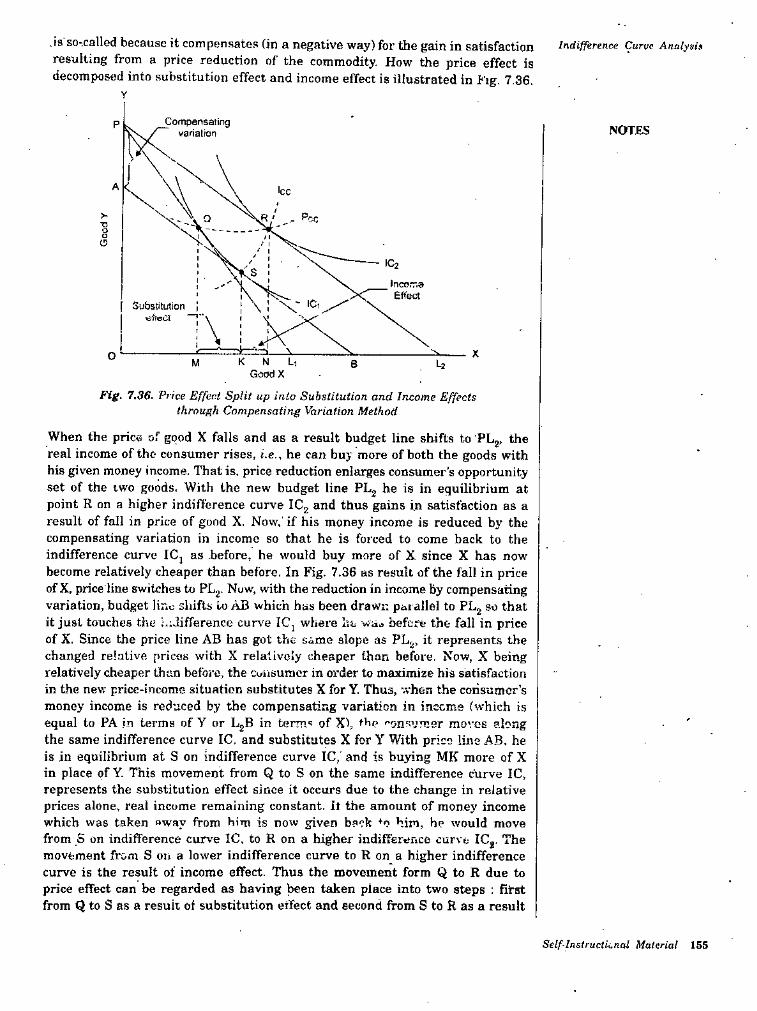
.is so-.called because it compensates (in a negative way) for the gain in satisfaction Indifference Curve Analysis resulting from adecomposed into substitution effect and income effect is illustrated in b'lg. 7.36,
price reduction of the commodity. How the price effect is
Compensatingvarialton
P NOTES
A
>-•DO
C5
IC2
IncomaEffea
SubstitutionwffeCI T\
XO K N GoodX
Fig. 7.36. Price Effect Split up into Substitution and Income Effects through Compensating Variation Method
When the price of good X falls and as a result budget line shifts to PLg, the real income of the consumer rises, i.e.. he can buy more of both the goods with his given money income. That is. price reduction enlarges consumer's opportunity set of the iwo goods. With the new budget line PLj he is in equilibrium at point R on a higher indifference curve ICg and thus gains in satisfaction as a result of fall in price of good X. Now. if his money income is reduced by the compensating variation in income so that he is forced to come back to the indifference curve ICj as .before, he would buy more of X since X has now become relatively cheaper than before. In Fig. 7.36 as result of the fall in price of X. price line switches to PLj- Now, with the reduction in income by compensating variation, budget line shifts lo AB which has been drawn parallel to PL^ so that it just touches the ;.;Jifference cur\'e ICj where ht wa., before the fall in price of X. Since the price line AB has got the same slope as PL^, it represents the changed relative prices with X relatively cheaper than before. Now, X being relatively cheaper than before, the cuiisumer in order to maximize his satisfaction in the new price-income situation substitutes X for Y. Thus, when the consumer’s money income is reduced by the compensating variation in incems (which is equal to PA in terms of Y or LjB in term' of X), '“onsumer moves along the same indifference curve IC, and substitutes X for Y With price line AB. he is in equilibrium at S on indifference curve IC,'and is bu3ring MK more of X in place of Y. This movement from Q to S on the same indifference curve IC, represents the substitution effect since it occurs due to the change in relative prices alone, real income remaining constant, it the amount of money income which was taken away from him is now given back *0 him, he would move from S on indifference curve IC, to R on a higher indifference curve IC^. The movement from S on a lower indifference curve to R on a higher indifference curve is the result of income effect. Thus the movement form Q to R due to price effect can be regarded as having been taken place into two steps : first from Q to S as a result of substitution eifect and second from S to R as a result
L,M L2B
Self-InsIructLnal Material 155
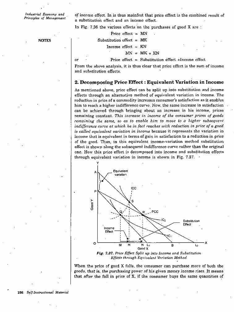
Industrial Economy and principles of Management
of income effect- In is thus mainfest that price effect is the combined result of a substitution effect and an income effect.In Fig. 7..36 the various effects on the purchases of good X are ;
Price effect = MN Substitution effect = MK
Income effect = KNMN = MK + .KN
Price effect = Substitution effect +Income effect From the above analysis, it is thus clear that price effect is the sum of income and substitution effects.
NOTES
or
2. Decomposing Price Effect; Equivalent Variation in IncomeAs mentioned above, price effect can be split up into substitution and income effects through an alternative method of equivalent variation in income. The reduction in price .of a commodity increases consumer’s satisfaction as it enables him to reach a higher indifference curve. Now, the same increase in satisfaction • can be achieved through bringing about an increase in his income, prices remaining constant. This increase in income of the consumer prices of goods remaining the same, so as to enable him to move to Q higher subsequent indifference curve at which he in fact reaches with reduction in price of a good is called equivalent variation in income because it represents the variation in income that is equivalent in terms of gain in satisfaction to a reduction in price of the good. Thus, in this equivalent income-variation method substitution effect is shown along the subsequent indifference curve rather than the original one. How this price effect is decomposed into income and substitution effects through equivalent variation in income is shown in Fig. 7.37. •
EquivalentvariationA
ICCP I((/> kS•o
'i8o /j
R ..PCCI
I ' J IC2I SubstitutionEffect
II
IIncome Effect'
I I
i\I
•ic,1)I
o N L,Good X
Fig. 7.37. Price Effect Split up into Income and Substitution Effects through Equivalent Variation Method
When the price of good X falls, the consumer can purchase more of both the goods, that is. the purchasing power of his given money income rises. It means that after the fall in price of X, if the consumer buys the same quantities of
M H LjB
156- Self.Instructionai Material
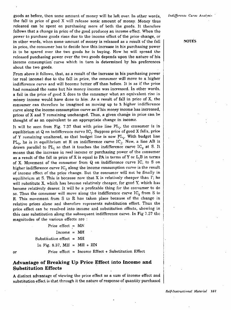
goods as before, then some amount of money will be left over. In other words, the fall in price of good X will release sonic amount of money. Money thus released can be spent on purchasing more of both the goods. It therefore follows that a change in price of the good produces an income effect. When the power to purchase goods rises due to the income effect of the price change, or in other words, when some-amount of money is released as a result of the fall in price, the consumer has to decide how this increase in his purchasing power is to he spared over the two goods he is buying. How he will spread the released purchasing power over the two goods depends upon the nature of his income consumption' curve which in turn is determined by his preferences about the two goods.From above it follows, that, as a result of the increase in his purchasing power (or real income) due to the fall in price, the consumer will move to a higher indifference curve and will become better off than before. It is as if the price had remained the same but his money income was increased. In other W'ords, a fail in the price of good X does to the consumer what an equivalent rise in money income would have done to him. As a result of fall in price of X, the consumer can therefore be imagined as moving up to S higher indifference curve along the income consumption curve as if his money income has increased, prices of X and Y remaining unchanged. Thus, a given change in price can be thought of as an equivalent to an appropriate change in income.It will be seen from Fig. 7.37 that with price line PLj. the consumer is in equilibrium at Q on indifference curve ICj. Suppose price of good X falls, price of Y remaining unaltered, so that budget line is now PI.,2- With budget line PLj, he is in equilibrium at R on indifference curve IC^. Now, a line AB is drawn parallel to PL; so that it touches the indifference curve ICj at S. It means that the increase in real income or purchasing power of the consumer as a result of the fall in price of X is equal to PA in terms of Y or L,B in terms of X. Movement of the consumer from Q on indifference curve IC, to S on higher indiffet^nce curve ICj along the income consumption curve is the result of income effect of the price change. But the consumer will not be finally in equilibrium at S, This is because now that X is relatively cheaper than 1’; he will substitute X, which has become relatively cheaper, for good Y, which has become relatively dearer. It will be a profitable thing for the consumer to do so. Thus the consumer will move along the indifference curve ICj from S to R. This movement from S to R ha.s taken place because of the change in relative prices atone and therefore represents substitution effect. Thus the price effect can be resolved into income and substitution effects, showing in this case substitution along the subsequent indifference curve. In Fig 7.37 the magnitudes of the various effects are :
Price effect = MN Income = MH
Substitution effect = MH In Fig. 8.37, MH = MH + HN
Price effect = Income Efiect + Substitution Effect
Indifference Curve Analysis
NOTES
or
Advantage of Breaking Up Price Effect into Income and Substitution Ejects
A distinct advantage of viewing the price effect as a sum of income effect and substitution effect is that through it the nature of response of quantity purchased
Self-Instructional Material 157
Industrial Ecniiomy and Principles of Management
to a change in the price of a good can be better and easily explained. In case of most of the goods, the income effect and substitution effect work in the same direction. But, in some cases, they may pull in different directions. The direction of substitution effect is quite certain. A fall in the relative price of a good always leads to the increase in quantity demanded of the good. In other words, substitution effect always induces the consumer to buy more of the cheaper good. But the direction of income effect is not so certain. With a rise in income, the individual will generally buy more of a good. But-with the rise in income the individual will buy less of a good if it happens to be an inferior good for him since he will use better or superior substitutes in place of the inferior good when his income rises. Thus the income effect may be either positive or negative. If for a good the income effect is positive, as is usually the case, it will act in the same direction as the substitution effect, that is, both will work towards increasing the quantity demanded of the good whose price has fallen. For the inferior good in which case income effect is negative, income effect of the price change will w’ork in opposite direction to the substitution effect. The net effect of the price change will then depend upon the relative strengths of the twd effects- To sum up, price effect is composed cf income effect and substitution effect and further that the direction in which quantity
• demanded will change as a result of’the fall in price will depend upon the direction and strength of the income effect on the one hand and strength of the substitution effect on the other.
, NOTES
PRICE-DEMAND RELATIONSHIP : DERIVING LAW OF DEMANDIndifference curve analysis with its technique of looking upon the price effect as a combination of income effect and substitution effect explains relationship between price and quantity demanded in a better and more analytical way. We explained above that the price effect shows the response of quantity demanded of a good to the changes in its price. We now proceed to derive from indifference- curve analysis a law oi'demand which should state in general tei'ms the relationship between price and quantity demanded of a good. In other words, we will try to derive a general demand theorem which describes the direction in which quantity demanded of the good will change as a result of a change in price of a good.In order to understand the way in which price-demand relationship is established in indifference curve analysis, consider Fig. 7,38. Given the price of two goods and his income represented by the budget line BLj, the consumer will be in equilibrium at Q on indifference curve ICj. Let us suppose that, price of X falls, price of Y and his money income remaining unchanged so that budget line now shifts to BLj. The consumer will now be in equilibrium at a point on the new budget line BL^. If the equilibrium position on BLj lies to the right of Q such as at R in Fig. 7.38, it will mean that the consumer buys more quantity of good X than at Q. And, if the equilibrium position on BLg, lies to the left of Q such as at H in Fig. 7.38, it will show that the consumer buys less of good'X than at Q. Now, it can be proved that the new equilibrium point on BL, will usually lie to the right of Q, meaning thereby that the quantity demanded of the good X will increase as its price falls.As seen above, the direction and magnitude of the change in quantity demanded as a result of the fall in price of a good will depend upon the direction and
158 Self-Instructional Material
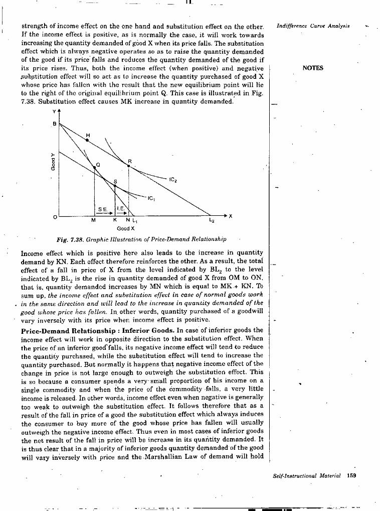
II.
strength of income effect on the one hand and substitution effect on the other. If the income effect is positive, as is normally the case, it will work towards increasing the quantity demanded of good X when its price falls. The substitution effect which is always negative operates so as to raise the quantity demanded of the good if its price falls and reduces the quantity demanded of the good if its price rises. Thus, both the income effect (when positive) and negative .substitution effect will so act as to increase the quantity purchased of good X whose price has fallen with the result that the new equilibrium point will lie to the right of the original equilibrium point Q. This case is illustrated in Fig. 7.38. Substitution effect causes MK increase in quantity demanded.
Indifference Curve Analysis
NOTES
Y
B
H
>R,Q
C3
SE.O K N L,
GoodX
Fig. 7.38. Graphic Illustration of Price-Demand Relationship
Income effect which is positive here also leads to the increase in quantity demand by KN. Each effect therefore reinforces the other. As a result, the total effect of a fall in price of X from the level indicated by BLj to the level indicated by BL^ is the rise in quantity demanded of good X from OM to ON. that is, quantity demanded increases by MN which is equal to MK.4 KN. To sum up, the income effect and substitution effect in case of normal goods work
. in the. same direction and will lead to the increase in quantity demanded of the good whose price has fallen. In, other words, quantity purchased of a goodwill vary inversely with its price when income effect is positive.Price-Demand Relationship : Inferior Goods. In case of inferior goods the income effect will work in opposite direction to the substitution effect. When the price of an inferior goocffalls, its negative income effect will tend to reduce the quantity purchased, while the substitution effect will tend to increase the quantity purchased. But normally it happens that negative income effect of the change in price is not large enough to outweigh the substitution effect. This is so because a consumer spends a verysmall proportion of his income on a single commodity and when the price of the commodity falls, a very little income is released. In other words, income effect even when negative is generally too weak to outweigh the substitution effect. It follows therefore that as a result of the fall in price of a good the substitution effect which always induces the consumer to buy more of the good whose price has fallen will usually outweigh the negative income effect. Thus even in most cases of inferior goods the net result of the fall in price will be increase in its quantity demanded. It is thus clear that in a majority of inferior goods quantity demanded of the good will vary inversely with price and the Marshallian Law of demand will hold
•-2M
Self-Instructional Material
Induttrial Economy and P'ineipUs of Management
1. Ordinal vs. Cardinal Measurability of Utility. In the first place, Marshall assumes utility to bo cardinally measurable. In other words, he believes that utility is quantifiable, both in principle and in actual practice. According to this, the consumer is able to assign specific amounts to the utility obtained by him from the consumption of a certain amount of a good or a combination of goods. Further, these amounts of utility can be added and compared in the some manner os weights, lengths, heights, etc.According to the critics, the as.sumption of cardinal measurement of utility is veiy strong, it demands too much from the human mind. They assert that utility is a psychological feeling and the cardinal measurement of utility assumed by Marshall and others is therefore unrealistic. Critics hold that the utility possesses only ordinal magnitude and cannot be expressed in cardinal terms. Therefore! the indifierence curve analysis assumes that utility is merely orderable and not quantitative. In other words, indifference curve technique assumes what is called 'ordinal meosi/rcmc/i/ of utility’. According to this, the consumer is capable of comparing different utilities or satisfactions in the sense whether one level of satisfaction is equal to, lower than, or higher than another. The advocates of indifference curve technique assert that for the purpose of explaining consumer’s behanour and deriving the law of demand, it is quite sufiicient to assume that the consumer is able to rank his preferences consistently. It is obvious that the ordinal measurement of utility makes a less strong assumption and sounds more realistic than cardinal measurement of utility. This shows that the indifference cur\'c analy.sis of demand which is based upon the ordinal utility hypothesis is superior to Marshall’s cardinal utility analysis.2. Analysis of demand without assuming constant marginal utility of money. Another distinct improvement made by indifference curve technique is that unlike Marshall it explains consumer's behaviour and derives demand theorem without the assumption of constant marginal utility of money. In indifference curve analysis, it is not necessary to assume constant marginal utility of money. It has already been seen, Marshall assumed that the marginal utility of money remained constant when there occurred a change in the price of a good. It has been shown in the last chapter that the Marshallian demand analysis based upon constancy of marginal utility of money is not applicable to multi-commodity model. In words, “the Marshallian demand theorem cannot genuinely be derived from the marginal utility hypothesis except in one commodity model, without contradicting the assumption of constant marginal utility of money. On the other hand, indifference curve technique using ordinal utility hypothesis can validly derive the demand theorem without the assumption of constant marginal utility of money, In fact, giving up the assumption of constant marginal utility of money enables the indifference curve analysis to enunciate a more general demand theorem,3. Greater insight into price effect. The superiority of indifference curve analysis further lies in the fact that it makes greater insight into the effect of the price change on the demand for a good by distinguishing between income and substitution effects. The indifference curve technique splits up the price effect analytically into its two component parts-substitution effect and income effect. The distinction •between the income effect and the substitution effect of a price change enables us to gain a better understanding of the effect of a price change on the demand for a good. The amount demanded of a good generally rises as a result of the fall in its price due to two reasons. First, because real income rises as a result of the fall in price (income effect) and, secondly, because the good whoso price
NOTES
1S4 Self-Instructional Material
falls becomes relatively cheaper than others and therefore the consumer substitutes it for others (substitution efTect).But, Marshall hy assuming constant marginal utility of money ignored the income effect of a price change. He failed to understand the composite character of the effect of a price change. Thus JR. Hicks writes, “The distinction between direct and indirect effects of a price change is accordingly left by the cardinal theory as an empty box, which is crying out to be filled. But it can be filled”. Further, Tapas Majumdar writes “The efficiency and precision with which Hicks- Allen approach can distinguish between the ‘income’ and ‘substitution’ effects of a price change really leaves the cardinalist argument in a very poor state indeed.4. Deriving a more general and adequate ‘demand theorem'. A distinct advantage of the technique of dividing the effect of a price change into income and the substitution effects employed by the indifference curve analysis is that it enables us to enunciate a more general and a more inclusive theorem of demand than the Marshallian law of demand. In the case of most of the normal goods in the world, both the income effect and the substitution effect work in the same direction, that is to say, they tend to increase the amount demanded when the price of a good falls. The income effect ensures that when the price of a good falls, the'eonsumer buys more of it because he can now afford to buy more of it; the substitution effect ensures that he buys more of it because it has now become relatively cheaper and is, therefore, profitable to substitute it for others. This thus accounts for the inverse price-demand relationship (Marshallian law of demand) in the case of normal goods.
' When a certain good is regarded by the consumer to be an inferior good, he will tend to reduce its consumption as a result of the increase in his income. Therefore, when the price of an inferior good falls, the income effect so produced
. would work in the opposite direction to that of the substitution effect. But so long as the inferior good in question does not claim a very large proportion of consumer’s total income, the income effect will not be strong enough to outweigh the substitution effect. In such a case therefore the net effect of the fall in price will be to raise the amount demanded of the good. It follows that even for most of the inferior goods, the Marshallian law of demand holds good as in case of normal goods.But it is possible that there may be inferior goods for which the income effect of a change in price is larger in magnitude than the substitution effect. This is the case of Giffen goods for which the Marshallian law of demand does not hold good. In such cases the negative income effect outweighs the substitution effect so that the net effect of the fall in price of the good is the reduction in demand for it. Thus, amount demanded of a Giffen good varies directly with price.It is clear from above that by breaking the price effect into income effect and substitution effect, the indifference curve analysis enables us to arrive at a general and a more inclusive theorem of demand in the following composite form :
Indifference Curve Analysis
NOTES
(a) The demand for a commodity varies inversely with price when the income efTect for that commodity is nil or positive as substitution effect is always present and tends to increase the quantity demanded of the commodity whose price falls and vice versa.
Self-Instructional Material 165
Industrial Economy and Principles of Management
(b) The demand for a commodity varies inversely with price when the income effect is negative but this negative income effect of the price change is smaller than the substitution effect.
(c) The demand for a commodity varies directly with .price when the income effect is negative and this negative income effect of the price change is larger than the substitution effect.
In the case of (a) and (6) the Marshallian law of demand holds while in case of (c) we have a Giffen good case which is exception to the Marshallian law of demand. Marshall could not account for ‘Giffen Paradox’. Marshall was not able to provide explanation for ‘Giffen Paradox’ because by assuming constant marginal utility of money, he ignored the income effect of the price change.5. Indifferp.nce curve analysis can explain substitute and complementaiy relationships between poods. Marshall’s cardinal utility analysis is based upon the hypothesis of independent utilities. This means that the utility which the consumer derives from any commodity is a function of the quantity of that commodity and of that commodity alone. In other words, utility obtained by the consumer from a commodity is independent of that derived from any other. By assuming independent utilities Marehall completely bypassed the relation of substitution and complementarily between commodities.Demand analysis based upon the hypothesis of independent utilities leads us to the conclusion “that in all cases a reduction in the price of one commodity only will either result in an expansion in the demand for all other commoditie.s or in a contraction in the demands for all other commodities”. But his is. quite contrary to the common cases found in the real world. In the real world, it is found that as a result of the fall in price of a commodity the demand for sow commodities expands while the demand for others contracts. We thus see that Marshall’s analysts based upon ‘independent utilities' does not take into account the complementary and substitution relations between goods. This is a great flaw in Marshall’s cardinal utility analysis.On the other hand, this flaw is not present in Hicks-Allen indifference curve analysis which does not assume independent utilities and duly recognizes the relation of substitution and complementarily between goods. Hicks-Allen indifference curve technique by recognizing interdependence of utilities is in a better position to explain related goods. By breaking up price effect into substitution and income effects by employing the technique of compensating variation income, Hicks succeeded in explaining complementary and .substitute goods in terms of substitution effect alone.6. Analysing consumer’s demand with less restrictive and fewer assumptions. It has been shown above that both the Hicks-Allen indifference curve theory and Marshall's cardinal theory arrive at the same condition for consumer’s equilibrium. Hicks-Allen condition for consumer's equilibrium, that is, MRS must be equal to the price ratio amounts to the same thing as Marshall’s proportionality rule of consumer's equilibrium. But even here indifference curve ordinal approach is an improvement upon the Marshall’s cardinal theory in so far as the former arrives at the same equilibrium condition with less restrictive and fewer assumptions. Dubious assumptions such as (i) utility is quantitatively measurable, (ii) marginal utility of money remains constant, and (Hi) utilities of different goods are independent of each other, on which Marshall's cardinal theory is based, are not made in indifference-curve’s ordinal utility theory.
NOTF.S
166 Self-Instructional Material
Is Indifference Curve Analysis “the Old Wine in a New Bottle”? Indifference Curve Analysis
But superiority of indifforence curve theory has been denied by some economists, foremost among thorn are Prof. D.H. Robertson, F.H. Knight, W.E. Armstrong. Prof. Knight remarks, ‘‘indifference curve analysis of demand is not a step forward; it is in fact a step backward.” Prof. D.H. Robertson is of the view that the indifference curve technique is merely “the old wine in a new bottle”. The indifference cun e analysis, according to him. has simply substituted new concepts and equations in place of the old ones, while the essential approach of the two types of analyses is the same. Instead of the concept of‘utility’, the indifference curve technique has introduced the term ‘preference’ and scale of preferences. In place of cardinal number system of one, two, three, etc., which is supposed to measure the amount of utility derived by the consumer, the indifference curves have the ordinal number system of first, second, third, etc., to indicate the order of consumer's preferences. The concept of marginal utility has been subsituated by the concept of marginal rate of substitution. And against the Marshallian 'proportionality rule’ as a condition for consumer’s equilibrium, indifference curv'c approach ha.s advanced the condition of equality between the marginal rate of substitution and the price ratio.
NOTES
Expressing the view that the concept of marginal rate of substitution in indifference curve analysis represents the reintroduction of the concept of marginal utility in demand analy.sis. Prof. Robertson says: “In his earlier book Value and Capital Hick’s treatment involved making an assumption about the convexity of those ‘indifference curves’ which appeared to some of us to involve reintroduction of marginal utility in disguise.” Thus, according to Prof. Robertson the use of marginal rate of substitution implies the presence of cardinal element in indifference
technique. In going from one combination to another on an indifference{. urvecurve, the consumer is assumed to be able to tell what constitutes his compensation in terms of a good for the loss of a marginal unit of’ another good, that is, he is able to tell his marginal rate of substitution of one good for another. Thus, it has, therefore, been held that the concept of marginal rate of substitution and the idea of indifference based upon it essentially involves an admission that utility is quantifiable in principle. However, this is hot correct interpretation ' of the concept of marginal rate of substitution. As Hicks has pointed out, we need not assume measurability of marginal utilities in principle in order toknow the marginal rate of .substitution. He says, “All that we shall be able to measure is what the ordinal theory grants to be measurable-namely the ratio of the marginal utility of one commodity to the marginal utility of another.” This means that MRS can be obtained without actually measuring marginal utilities. If a consumer, when asked, is prepared to accept 4 units of good Y for the loss of one marginal unit of X, MRS of X for Y is 4 : 1. ‘We can thus directly derive the ratio indicating MRS without measuring marginal utilities by offering him how much compensation in terms of good Y the consumer would accept for the loss of a marginal unit of X.It has been further contended by Robertson and Armstrong that it is not possible to arrive at the Hicksian principle of diminishing marginal rate of substitution without making use of the ‘Marshallian framework’ of the concept of marginal utility and the principle of diminishing marginal utility. It is asked why MRS of X for Y diminishes as more and more of X is substituted for Y? The critics point out that the marginal rate of substitution (MRS) diminishes and the indifference curve becomes convex to the origin, because as the consumer’s stock of X increases, the marginal utility of X falls and that of Y increases. They thus hold that Hicks and Allen have not been able to derive the basic
Self-Instructional Material 167
Industrial Economy and Principles of Management
principle of diminishing marginal rate of substitution independently of the law of diminishing marginal utility. They contend that by a stroke of terminological manipulation, the concept of marginal utility has been relegated to the background, but it is there all the same. They, therefore, assert that “the principle of diminishing marginal rate of substitution is as much determinate or indeterminate as the poor law of diminishing marginal utility”.However, even this criticism of indifference curve approach advanced by the defenders of the Marshallian cardinal utility analysis is not valid. As shown • above, the derivation of marginal rate of substitution does not depend upon the actual measurement of marginal utilities. While the law of diminishing marginal utility is based upon the cardinal utility hypothesis iLe., utility is quantifiable and actually measurable), the principle of marginal rate of substitution is based upon the ordinal utility hypothesis (t.e., utility is mere crdorable). As a consumer gets more and more units of good X, his strength of desire for it (though we cannot measure it in itself) will decline and therefore he will be prepared to . forgo less and less of Y for the gain of a marginal unit of X.It is thus clear that the principle of diminishing marginal rate of substitution is based upon purely ordinal hypothesis and is derived independently of cardinal concept of marginal utility, though both laws reveal essentiaUy the same phenomenon. The derivation of the principle of diminishing marginal rate of substitution by using ordinal utility hypothesis and being quite independent of the concept of marginal utility is a great achievement of the indifference curve analysis. We therefore agree with Prof. Hicks who claims that “the replacement of the principle of diminishing marginal utility by the principle of diminishing marginal rate of substitution is not a mere translation. It is a positive change in the theory of consumer’s demand”.It follows from what has been said above that indifference curve analysis of demand is an improvement upon the Marshallian utility analysis and the objections that the former too involves cardinal elements are groundless. It is of course true that the indifference curve analysis suffers from some drawbacks and has been criticized on various grounds, as explained below, but as far as'the question of indifference curve technique versus Marshallian utility analysis is concerned, the former is decidedly better.
NOTES
CRITIQUE OF INDIFFERENCE CURVE ANALYSISIndifference curve analysis has come in for criticism on several grounds. In the first place, it is argued that the indifference curve approach for avoiding the difficulty of measuring utility quantitatively, is forced to make unrealistic assumption that the consumer possesses complete knowledge of his whole scale of preferences or indifference map. The indifference curve approach, so to say. falls from the frying pan into the fire. The indifference curve analysis envisages a consumer who carries in his head innumerable possible combinations of goods and relative preferences in respect of them. It is argued: Is not this carrying into his head all his scales of preferences too formidable a task for a real human being? Hicks himself admits this drawback. When revising his demand theory based on indifference curves, he says that “one of the most awkward of the assumptions into which the older theory appeared to be impelled by its geometrical analogy was the notion that the consumer is capable of ordering all conceivable alternatives that might possibly be presented to him-aU the positions which might be represented
168 Self-Instructional Material
by points on his indifTerence map. This assumption is so unrealistic that it was bound to be a stumbling block." This is one of the reasons why Hicks has given up indifference curves in his Revision of Demand Theory.Further, another unrealistic element is present in indifference curve analysis. It is pointed out that such curves include even the most ridiculous combinations which may be far removed from his habitual combinations. For example, while it may be perfectly sensible to compare whether three pairs of shoes and six shirts would give a consumer as much satisfaction as two pairs of shoes and seven shirts, the consumer will be at a loss to know and compare the desirability of an absurd combination such as eight pairs of shoes and one shirt. The way the indifTerence curves are constructed, they include absurd combinations like the one just indicated. A further shortcoming of the indifference curve technique is that it can demonstrate and analyses consumer's behaviour effectively only ih simple cases, especially those, in which the choice is between the quantities of two goods only. In order to demonstrate the case of three goods, three- dimensional diagrams are needed which are difficult to understand and handle. When more than three goods are involved, geometry altogether fails and recourse has to be made to the complicated mathematics which often tends to conceal the economic aspect of what is being done. Prof Hicks also admits this shortcoming of indifference curve technique.Another demerit of the geometrical nature of indifference curve analysis is that it involves the assumption of continuity “a property which the geometrical field does have, but which the economic world in general does not”. The real economic world exhibits discontinuity and it is quite unrealistic and analytically bad if we do not recognize it. This is why Hicks too has given up the assumption of continuity in his later work A Revision of Demand Theory.
■ Another important criticism against Hicks-Allen ordinal theory of demand is that it cannot formalise consumer’s behaviour when uncertainty or risk is present. In other words, consumer’s behaviour cannot be explained by ordinal utility theory when he has to choose among alternatives involving risk or ‘uncertainty of expectation’. Von Neumann and Morgenstern and also Armstrong have asserted that while cardinal utility theory can, the ordinal utility theory'- cannot formalise consumer’s behaviour when we introduce “uncertainty” of expectations with regard to the consequences of choice.”Further, Prof Samuelson has criticized the indifference curve approach for being predominantly introspective. Prof, Samuelson himself has developed a behaviorist method of deriving the theory of demand. He seeks to enunciate demand theorem from observed consumer’s behaviour. He regards the behavioristic approach, as being ‘scientific’. His theory is based upon the strong-ordering hypothesis, namely, ‘choice reveals preference.’ Samuelson thinks that his theory removes the last vestiges of the psychological analysis in the explanation of consumer’s demand.
Indifference Curve Analysis
NOTES
Self-Instructional Material 169

Industrial Economy and Principles of Management
STUDENT ACTIVITY
1. State and illustrate the concept of indifference curve by preparing an imaginary indifference schedule.
2. What is an indifference curve ? What are its properties ? Discuss in brief.
170 Self-Instructional Material
Indifference Curve'. AnalysisSUMMARY• The indifference curve method seeks to derive all rules and laws about
consumer’s demand that are derivable from the cardinal utility analysis.• The fundamental approach of indifference curve analysis is that it has aban
doned the concept of cardinal utility and instead has adopted the concept of ordinal utility.
• A consumer is said to be in equilibrium when he is buying such a combination of goods as leaves him with no tendency to rearrange his purchases of goods.
• Indifference curve analysis with its technique of looking upon the price effect as a combination of income effect and substitution effect explains relationship between price and quantity demanded in a better and more anal5d;ical way.
• Price consumption curve traces the effect of a change in price on the quantity demanded of a good. But price consumption curve does not directly relate price with quantiQf demanded.
NOTES
REVIEW EXERCISES1. Explain the features of indifference curves. Why does an indifference
curve slopes downward ?2. What is a budget line ? Examine the effect on a budget line of (i)
change in income and (ti) change in prices.3. At what point on an indifference curve does a consumer maximise
his satisfaction? Explain with the help of a diagram.4. Draw indifference curves in case of (o) perfect substitutes, and (6)
perfect complements.5. Explain consumer’s equilibrium using indifference curve analysis.
• 6., Discuss the assumptions on'which the indifference curve analysis is based.
7. What is indifference map ? How will you prove that higher indifference curve represents higher level of satisfaction ?
8. Briefly explain the exceptions to the properties of indifference curve.9. Explain graphically the concept of Budget Line and discuss the effect
of change in price and income on budget line.10. Explain consumer’s equilibrium under the indifference curve analysis. H. Discuss the superiority of indifference curve approach over the marginal
utility analysis.12. Answer the following :
(o) What is an indifference curve ?(6) What are perfect substitutes ?(e) What is indifference map ?(d) Explain the effect of change in income on budget line.(e) Show with the help of a diagram the impact of change on price on
budget line.
Self-Instructional Material 171
SecHon-C : MONEY AND BANKING Nature and Function,s of Monty
UNIT 8 NATURE AND FUNCTIONS
OF MONEY NOTES
★ STRUCTURE ★□ Introduction and Concept'
□ Nature, Features and Characteristics of Money
INTRODUCTION AND CONCEPTMoney may be any commodity chosen by common consent as a medium of exchange. It is expected in payment for goods and services and in settlement of debts. .It is given and received without reference to the person who is using it. For instance, a rupee note is a rupee note whether it is used by the ' President of India or by a blind beggar in the street."The real significance of money is that it is a claim which can be used'by its owner to buy anything."“Anything that is commonly used and generally accepted as a medium of exchange or as a standard of value".
—A-C.L. Day
—Raymond P. Kent‘Thing which possess general acceptability". —Seligman‘Anything which is widely accepted tn payment for goods, or in discharge of
—Robertsonother kinds of business obligation.""Money can be defined as, anything that is generally acceptable as a means of exchange (i.e., as a means of settling debts) and that of the same time acts as a measure and as a store of value.In short, it can be said that money is any commodity which is generally , accepted as a medium of exchange, standard of value, store of value and a standard of deferred payments. Anything which is used as money should have the follon’ing features ;
1. It should pass from hands to hands that is, it should be received regularly with the idea of offering it in payment to others.
2. It should be used to buy and sell all goods and services.3. It can be anythii^—a useful or useless commodity, a metal (like gold
or silver), a piece of paper fe.g., a currency note).4. It should be used to buy or sell all goods and services.
—Crowther
NATURE, FEATURES AND CHARACTERISTICS
OF MONEYFeatures and characteristics of money are as follows :
1. Money acts as a store of value.2. Money facilitates exchange.
Self-Instructional Material 173
Industrial Economy and Principles of Management
3. Money is also used as standard of value.4. Money facilitates deffered payments. ■5. Money in any commodity have general acceptance.6. Money has generalised purchasing power.
NOTESFunctions of MoneyIn the views of Crowther, “the only essential requirement of money is general acceptability”. According to Walker, “Money is what money does". Money is known for what it does or performs.Money was introduced to overcome the difllculties of the barter system and to help in exchange. The functions of money can be summarized by the following poinUs :
1. Money is a standard for measuring values.2. Money serves as a medium of payment.3. Money as a means of a transferring value.4. Money is used as a store of value i.e., it keeps the resources liquid.5. Money as a medium of exchange.6. Money serves as a standard for deferred payments.1. Money is a standard for measuring values. When money serves as a
medium of exchange, it incidently measures the value of things for which it is exchanged. One inconvenience of barter, was the lack-of common measure or a common denominator of value in terms of which other values could be expressed and added and accounts kept. Money removes this difficulty too. Money serves as a unit of account. In a money economy, it is easy to compare the relative values of commodities and services which are dissimilar and entirely different from one another. The values are in proportion to their respective prices. Expression of value in prices enables us to add them up and have a definite idea of person’s or a community’s wealth. In matters of exchange, a common standard of value makes the transaction easy and also fair.
2. Money serves as a medium of payment. Money is a medium of payment, that is. it is used to make and receive all payments. A commodity is bought and sold with the help of money and it is also paid for in money. The function of money as a medium of payment is implied in the above function of money as a medium of exchange.
■ 3. Money as a means of transferring value. There is also another function which money performs. One can sell one’s immovable and movable belongings at one place and with the money so acquired he can buy them elsewhere, value will then be transferred. Such things have happened on a very large scale in India after the partition of the country.
4. Money is used as a store of value i.e., it keeps the resources liquid. Money serves as a-store of value or more correctly i.e., enables a person to keep a portion of his assets liquid. Liquid assets are those which can be used for any purpose at any time one likes. Most persons in the modern world have to keep currency notes in their packet or at home, or they may keep current accounts with the'
174 Self-Instructional Material
Nature and Functions of Money
banks withdrawable by cheque. The necessity arises from the fact that the two streams of income and expenditure do not keep time with each other. An employer has to pay wages, etc., periodically; even daily, while his income does not come to him in the same periodical intervals. Money is best kept as a store of value to he used as and when need arisesMoney as a medium of exchange. The first and the most important function .of money is to help in buying and selling of goods and services. Commodities are not exchanged directly but are exchanged through money. In case of farmer, the farmer sells his produce in the market for money, He uses this money to buy clothes, pulses, rice, matches, sugar and other things which he requires. A teacher who sells his services to the college for money: he uses his money to buy all kinds of goods and services which he requires. Thus, money is the medium of exchange or medium of trade.Money serves as a standard for deferred payments. Money helps us to buy goods and services not only in the present but also in the future. Suppose a person buys a pen from a shop and pays him money immediately. This is cash transaction. Suppose, instead, he buys a pen now and agrees to pay later it becomes a credit transaction. Further, if a person borrows from a moneylender and agrees to return the amount later, it is also credit transaction. Money helps to buy and sell or borrow and lend. In other words, money serves as a standard of deffered payment.
NOTES5.
6.
Defects and Drawbacks of MoneyThough money plays an important and essential part in the economy of a country, it would be wrong to conclude that money is the cause of all economic changes and progress. Money is only an instrument which helps in economic progress but it is not the controlling authority. Money is a good servant but a bad master. Money can be proved dangerous in several ways :
Money leads to corruption.Money leads to inequalities of incomes.Money has instability.Money leads to corruption. Money has been -responsible for all the corruption which is prevalent in modern society. As Ruskin stated; “The devil of money has come to possess their souls. No religion or philosophy seems to have the power of driving it out”. Money is regarded as the cause of theft and murder, of deception and betrayal. It is the lust for money which induces man to go for illegal and dubious means of accumulating money.Money leads to inequalities of incomes. Money has proved to be a very convenient tool for amassing wealth and of the exploitation of the poor by the rich. It has created a yawning gulf between the ‘haves’ and the ‘have nots’. The misery and degradation of the poor is thus, to no small measure due to the existence of money.Money has instability. A very great defect of money is that its value or purchasing power does not remain stable or constant. Different sections of people in the country are affected differently because of changes in the value of money. For instance, a fall in the value of
1,2.3,1,
2.
3.
Self-Instructional Material 176
IltduRtrial BcoTumiy and Principles of Management
money (inflation) leads to wrong distribution of income since the rich become richer while the poor becomes poorer. A rise in the value of money (deflation), meaning a fall in prices and decline in employment may lead to great suffering to all classes of people.
NOTES Role, Importance and Significance of Money in Modern Economy'I'herc is no doubt that money facilitates and motivates all economic activities relating to consumption, production, exchange and distribution. Money enables a consumer to maximize hi.s satisfaction. Money measures' the intensity of desire and the utility of commodity to a consumer. The role and significance of money in modern economy can be summarii.ed Ly the ihllowing points :
1- Significance of money in production. Without mone3\ production on the modern scale would bo impossible. The present day industrial production is based on extreme division of labour or specialisation which implies that the worker cannot be paid in the commodity he produces and also the existence of the extensive market to dispose off commodity. It is money which has made possible the extreme specialisation and, therefore resulted in large-scale production.Again, money enables every man to concentrate his attention on his own job, without bothering about all other things and thus to add more effectively to the general flow of goods and services which constitute the real income of societyIt is clear, therefore, that without money, modern specialisation is impossible and without specialisation modern capitalist economy could not have come into existence.The martufacturers use money to purchase materials for the construction of their factories, they use it to buy the materials necessary for their equipments. They bid competitively in the markets of the world for the raw materials used in the process of manufacturing- They employ money as a means of attracting to their business the requisite labour force, officials and professionals.
2. Significance of money in consumption. The consumer receives his income in the form of money, which he can convert .into anything he likes. A worker in a cloth factory cannot be paid in a cioth or an employee in a shoe factory in shoe-. It is impossible for workers to go about exchanging cioth or shoes for rice, wheat, vegetables and hundreds of old things they require. When payment is made in kind {and not in money) there is high possibility that the consumer gets too much of some goods and too little of others. The consumer, therefore, does not get maximum satisfaction in the absence of money. On the other hand, when the consumer receives his income in the form of money, he can distribute it on the different goods in such a way that lus total satisfaction will be highest The use of money and the system of-prices give the consumers the necessary freedom to choose and substitute between goods and serrices. It is the .system of money and prices which help the to (q) choose the type of goods they consume; (fc) the variety of goods they can choose; and (c) the amount which they could choose.
3, Money as medium of exchange. One important reason why money occupies a central position in a modern economy is the function of money
consumers
as a
176 Self-Instructional Material
Natui'^ ond Functioim of Moneymedium of exchange, and of payments. Everything can be bought and
sold, i.e., exchanged through the medium pf money. Goods and services are exchanged through money. Shares aiid bonds (which are known as claims to wealth) are bought and sold in the form of money. Similarly, taxes to the government are paid in money. In other words, money is used as the general medium of exchange and of payment. Without it, there can be no trade and, therefore, no production. (In modem economy, there can be no production, if what is produced cannot be sold).
4. Significance of money to the modern state. The government is a large receiver as well as maker of payments. The state receives income by way of taxes, fees, fines, prices for service rendered etc. The income which the states get may be one-third or one-forth of the total national income. It is impossible to collect taxes, fees, fines, etc., in the forms of goods. The farmer would pay in grains; the cobbler in shoes, the carpenter in chairs and tables; and so on. This would create problems of collection, storage or distribution. Similarly, the government has to make payment by way of wages, salaries, interest, etc. This would be impossible except in terms of money. Public revenues and public expenditures are so vast that they are possible'only in a money economy. Moreover, modern governments plan their incomes and expenditure in advance. This would not bo possible if they collect their revenue to kind. Revenues received in goods and payments made in kind would make calculation and budgeting an impossible task.
5. All incomes are in the form of money. All incomes that are received are in the form of money. This necessarily follows from the fact that money serves as a general medium of exchange and of payments in settlement of debts. The firms which sells its goods, receives money for it; its income, therefore, consists of money. The lacturer who sells his services to the college gets his salary in the form of money Since all payments are made in money, every income is a money income (payment by one person becomes income for another). Thus, in a modern economy, all incomes are money incomes.
NOTES
6. Significance of money in trade. The basic purpose of money is to help in the exchange of goods and services (i.e., trades). In a primitive economy, there was very little trade. Naturally, the system of exchange
barter. With extension of trade, the need for money rises. Large-wasscale production and extension of markets to sell the goods produced are impossible without the use of money. In the last two hundred years, trade has become very extensive and to facilitate this, new types of money have been involved. The use of bank cheques and bank drafts ■ facilitates buying and selling of goods as well as of payments.Not only internal trade, but international trade too is possible only through money The currency of one country may be acceptable in India but cannot buy even a match box in England or the U.S.A. However, trade between two countri'’? is financed by means of bank drafts.
■ Itade, both interna! and international, is very important and indispensable for modern large-scale production. Money is the medium by which trade is undertaken. If there were no money, there would be no extensive trade; if there were no trade, there would be no large-scale production and no modern capitalist economy.
Self-Instructional Material 177
hidualrial Economy and 'Principles of Management 7- Wealth kept partly in money. Another important factor responsible for
the central position of money in modern times is that money constitutes the most important form of wealth. Everyone i.e., individual, company or corporation or the government wishes to have some cash to meet current obligations and as a precautionary measure (for reserves). The amount of cash held by people will naturally differ from individual to individual and from institution to institution. A rich man will obviously keep more cash than a poor man. But everyone keeps some cash with himself or as deposit in a bank.
NOTES
178 Self-Instructional Material
Nature and Functions of Money
STUDENT ACTIVITY
1. “Money is what money does." Explain what are the different forms of money in use of modern times.
2. Explain the various .fiinctions of money. How do these functions remove the difficulties of the barter system?
Self-Instructional Material 179
Industrial Economy and Principles of Management SUMMARY
• Money was introduced to overcome the difficulties of the barter system and to help in exchange.
• When money serves as a medium of exchange, it incidently measures the value of things for which it is exchanged,
• Money is a medium of payment, that is, it is used to make and receive all payments.
• Though money plays an important and essential part in the economy of a country, it would be wrong to conclude that money is the cause of all economic changes and progress.
NOTES
REVIEW EXERCISES1. Describe the functions of money. Bring out its importance in economic
• Ufe,2. Describe the defects and drawbacks of money.3. Explain the role and significance of money in modern economy.
180 Self-Instructional Material
Value of Money
UNIT 9 VALUE OF MONEY
★STRUCTURE ★ NOTES
□ Introduction and Concept
□ Measurement of the Value of Money/Index Number of Prices
□ Procedure of Calculating the Index Number of Prices
INTRODUCTION AND CONCEPTValue of money means the buying capacity of money. It shows the purchasing power of money over commodities and services. It denotes the capacity of money to buy commodities and services. It refers to the volume of goods and services which a unit of money will buy at a given line and place. When a unit of money purchases larger amount of commodities and services, its value is said to be higher and vice versa.Since the number of commodities and services are available for exchange with money is very large, it is very difficult to express the value of money in terms r ■ me particular commodity. Therefore, the value of money cannot be expressed oniy relatively. There is an inverse relationship between the price-level and the value of money. The buying capacity of money is always dependent on the price-level. When the price-level rises, money buys less and, therefore, we say the value of money has fallen. Similarly, when the price level falls, value of money rises. The variation in the value of money is always accompanied by opposite variation in the prices of commodities and services. In brief, value of money varies inversely with the price-level. It is reciprocal of price level.
V„ = 1m pwhere denotes the value of money, and P stands for price level.
MEASUREMENT OF THE VALUE OF MONEY/ INDEX NUMBER OF PRICESValue of money does not remain stable over a long period of time. It goes to changing as the price-level changes in the economy. The changes in the value of money are measured by constructing the Index numbers. The value of everything is measured in terms of money. But the value of money cannot be measured in terms of money. Money is generally wanted for the purpose, of bringing goods and services. Therefore, the value of money can be ascertained by averaging the prices of number of selected commodities on which people spend their income. The average of the prices of commodities and services on which a large chunk of money income is spent gives us the price-level and a series of such price level is known as the Index Numbers. In other words, the
Self-Instructional Material 181
Industrial Econ6my and Prineiples of Sianautment changes in the value of money can be measured only indirectly with the help
of index numbers.
Index Number. An index number is a device to measure changes in the level of any economic phenomenon. In a dynamic setting changes occur very often and therefore, it is necessary to measure their direction and extent. It is likely that the prices may change over a period of time or even production and wages may undergo changes witli the passage of time. All such changes can be measured with the help of Index Numbers.Index number is essentially a mathematical device used to measure changes in the prices level. Index number of prices is a number representing the average price of selected group of commodities and services at a particular point of time. This number is always expressed comparatively i.e., in relation to the average price of the same group of commodities at some other time. Even though it is possible to measure the value of money in relative terms, there are certain practical limitations. First, prices of all commodities and services do not rise uninformaily. Second, people are not interested .in the changes of prices of all commodities.TVpca of Index Numbers : Different types of index numbers are as follows:1. Retail prices index number.2. Wholesale prices index number.3. Working class cost of living index number.4. General purpose index number.5. Consumption goods index number.
1. Retail prices index number. The goods exchanged in the retail market and their prices are taken into consideration for constructing the index number of retail prices. Such type of index number shows the price movement in the retail market and their effect on the consumers. The essential for the construction of this type of index number is that the retail prices of the same goods and changes in them should be available accurately. The need for accurate statistic-s can hardly be exaggerated.
2. Wholesale prices index number. This type of index number is computed to measure the prices of commodities traded in the wholesale market. Since their general purpose index number is difficult to construct, the index number of wholesale prices is made use of as an index to measure the value of money in general. The goods transacted in the wholesale market and their prices are taken into consideration in constructing the index number of wholesale prices.
3. Working class cost of liuing index number. The goods and services consumed by the working class and their prices are taken into consideration while constructing the working class of living index number. This index number obviously shows the value of goods and services consumed by the working class. The working class cost of liNing index number reflects the cost of living of workers. In a well-developed industrialised economy, this type of index number plays a very significant role as the demand for higher wages by the industrial workers depends upon
NOTES
182 Selflruiruftional Material
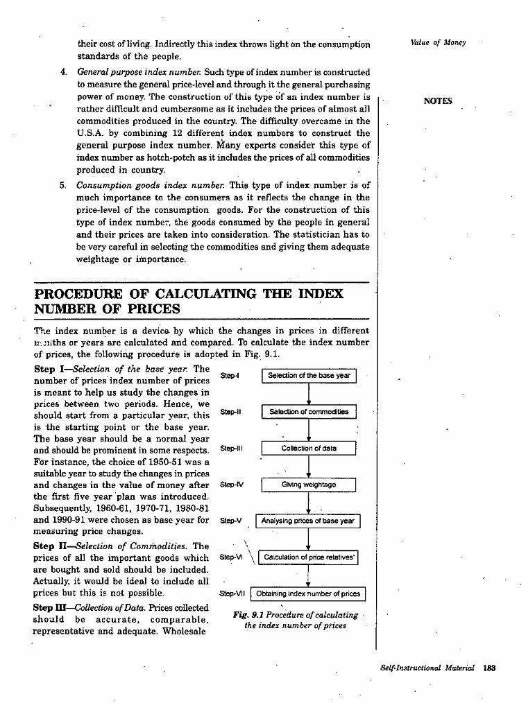
their cost of living. Indirectly this index throws on the consumption standards of the people.
4. General purpose index number. Such type of index number is constructed to measure the general price-level and through it the general purchasing power of money. The construction of this type of an index number is rather difTicult and cumbersome as it includes the prices of almost all commodities produced in the country. The difficulty overcame in the U.S.A. by combining 12 different index numbers to construct the general purpose index number. Many experts consider this type of index number as hotch-potch as it includes the prices of aU commodities produced in country.
5. Consumption goods index number. This type of index number is of much importance to the consumers as it reflects the change in the price-level of the consumption goods. For the construction of this type of index number, the goods consumed by the people in general and their prices are taken into consideration. The statistician has to be very careful in selecting the commodities and giving them adequate weightage or importance.
Value of Money
NOTES
PROCEDURE OF CALCULATING THE INDEX NUMBER OF PRICESThe index number is a device by which the changes in prices in different mjiiths or years are calculated and compared. To calculate the index number of prices, the following procedure is adopted in Fig. 9.1.Step I—Selection of the base year. The number of prices index number of prices is meant to help us study the changes in prices between two periods. Hence, we should start from a particular year, this is the starting point or the base year.The base year should be a normal year and should be prominent in some respects.For instance, the choice of 1950-51 was a suitable year to study the changes in prices and changes in the value of money after the first five year plan was introduced.Subsequently, 1960-61, 1970-71, 1980-81 and 1990-91 were chosen as base year for step-v measuring price changes.Step n—Selection of Commodities. The prices of all the important goods which Siep-vi are bought and sold should he included.Actually, it would be ideal to include all prices but this is not possible.Step in—Collection of Data. Prices collected should be accurate, comparable, representative and adequate. Wholesale
Selection of Uie base yearStep-l
Selection of commoditiesStep-ll
St^III Collection of data
Step-lV Giving weightage
Analysing prices of base year
Calculation of price relatives'
Step-VII Obtaining index number of prices
Fig. 9.1 Procedure of calculating the index number of prices
Self-Instructional Material 183
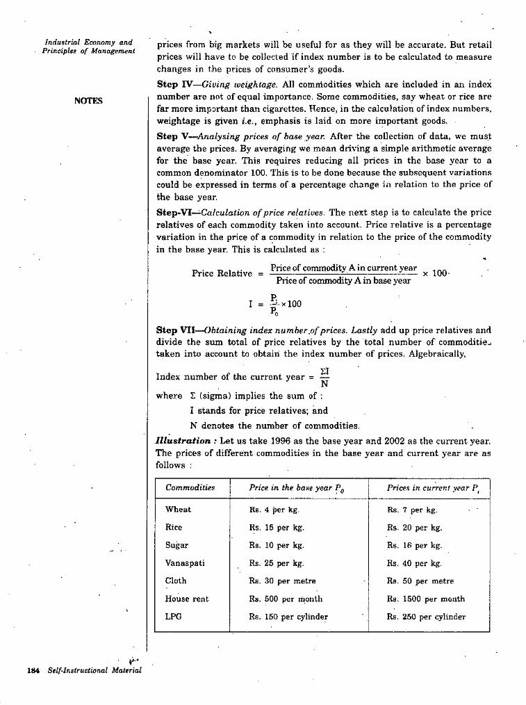
Industrial Economy and ■ Principles of Management prices from big markets will be useful for as they will be accurate. But retail
prices will have to be collected if index number is to be calculated to measure changes in the prices of consumer’s goods.Step IV—Giving weightage. All commodities which are included in an index number are not of equal importance. Some commodities, say wheat or rice are far more important than cigarettes. Hence, in the calculation of index numbers, weightage is given i.e., emphasis is laid on more important goods.Step V-^Analysing prices of base year. After the collection of data, we must average the prices. By averaging we mean driving a simple arithmetic average for the base year. This requires reducing all prices in the base year to a common denominator 100. This is to be done because the subsequent variations could be expressed in terms of a percentage change in relation to the price of the base year.Step»VI—Ca/cu/ation of price relatives. The next step is to calculate the price relatives of each commodity taken into account. Price relative is a percentage variation in the price of a commodity in relation to the price of the commodity in the base year. This is calculated as ;
NOTES
Price of commodity A in current yearPrice Relative X 100Price of commodity A in base year
I = -^xlOOPo
Step VII—Obtaining index number.of prices. Lastly add up price relatives and divide the sum total of price relatives by the total number of commoditie.. taken into account to obtain the index number of prices. Algebraically,
SIIndex number of the current year = —
where I (sigma) implies the sum of;1 stands for price relatives; and N denotes the number of commodities.
Illustration : Let us take 1996 as the base year and 2002 as the current year. The prices of different commodities in the base year and current year are as follows :
Commodities Price in the base year Pg Prices in current year P,
Wheat Rs. 4 per kg. Rs- 7 per kg.
Rice Rs. 15 per kg.
Rs. 10 per kg.
Rs. 25 per kg.
Rs. 20 per kg.
Rs. 16 per kg.
Rs. 40 per kg.
Sugar
Vanaspati
Cloth Rs. 30 per metre Rs. 50 per metre
Rs. 500 per month
Rs. 150 per cylinder
House rent Ra. 1500 per month
Rs. 250 per cylinderLPG
184 Self-Instructional Material
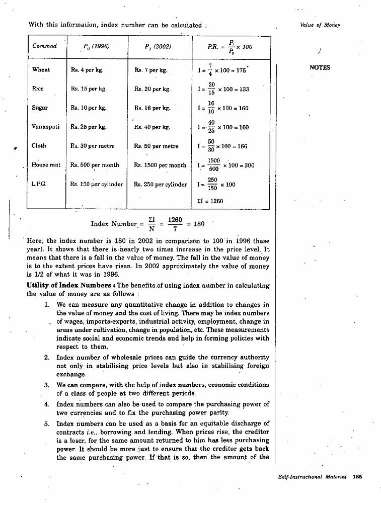
With this information, index number can be calculated : Value of Money
P.R. = 100Commod (1996) P, (2002)■JPc
7 NOTESWheat Ra. 4 per kg. Rs. 7 per kg. 7 X 100 = 175 4
20Rice Rs. 15 per kg. Ra. 20 per kg. 1= TT X 100 = 13315
16Sugar Rs. 10 per kg. Rs. 16 per kg. 1 = TT X 100 = 16010
40Vanaspati Rs. 25 per kg. Rs. 40 per kg. .1 = X100 = 16025
50Cloth Rs. 30 per metre Rs. 50 per metre 1= t;tx100 = I66r 30
1500House rent Rs. 500 per month Rs. 1500 per month 1 = X100 = 300500
250L.PG. Rs. 150 per cylinder Rs. 250 per cylinder 1 = X 100150
11 = 1260
ZI 1260Index Number = = 180N 7
Here, the index number is 180 in 2002 in comparison to 100 in 1996 (base year). It shows that there is nearly two times increase in the price level. It means that there is a fall in the value of money. The fall in the value of money is to the extent prices have risen. In 2002 approximately the value of money is 1/2 of what it was in 1996.
Utility of Index Numbers : The benefits .of using index number in calculating the value of money are as follows :
1. We can measure any quantitative change in addition to changes in the value of money and the.cost of living. There may be index numbers
. of wages, imports-exports, industrial activity, emplosTnent, change in areas under cultivation, change in population, etc. These measurements indicate social and economic trends and help in forming policies with respect to them.
2. Index number of wholesale prices can guide the currency authority not only in stabilising price levels but also in stabilising foreign exchange.
3. We can compare, with the help of index numbers, economic conditions of a class of people at two different periods.
4. Index numbers can also be used to compare the purchasing power of two currencies and to fix the purchasing power parity.
5. Index numbers can be used as a basis for an equitable discharge of contracts i.e., borrowing and lending. When prices rise, the creditor is a loser, for the same amount returned to him has less purchasii^ power. It should be more just to ensure that the creditor gets back the same purchasing power. If that is so, then the amount of the
Self-Instructional Material 185
Industrial Economy and Principles of Management
principal should be increased in proportion to the increase in prices. Similarly, when the prices fall, the debtor should be asked to pay correspondingly less, otherwise the burden of the debt in terms of commodities and services will be increased in proportion to the fall in prices.
‘ 6. The method of index numbers is used for measuring changes in the price-level. This is essential for maintaining price stability. Price stability is conducive to the maintenance of economic activity at the desired level.
7. An index number of cost of living can guide us in the adjustment of wages to changing price.
Limitations and DiMculties in Calculating Index Numbers : Although index numbers provide a fairly broad guidelines to devise suitable policies of economic welfare and development, but it is not possible to measure accurately the changes in the value of the money due to following limitations : '
1. The introduction of new goals which may act as close substitutes for old and high priced commodities cannot be taken into consideration.
2. The selection of weights is arbitrary and based upon the personal •inclination of the statistician.
3. Changes in the quality of commodities and services cannot be taken into consideration.
4. The index numbers of different places are hardly comparable because the significance of prices to consumption varies according to task, habits, climates and such other factors.
5. The uniformity of basis necessary for comparison between different years may not always exist. Hence, it is difficult to draw any inference by comparing index number by a long period of time.
NOTES
Self-InstriiCtiondl Matirial
Value of Money
STUDENT ACTIVITY• .1. What do you understand by value of money ? How the value of money is measured?
\
2. What do you understand by index numbers ? Discuss the various types of index numbers.
Self-2n$tructional Material 187
IndMtriat Economy and Principles of Management SUMMARY
• When the price-level rises, money buys less and, therefore, we say the value of money has fallen. Similarly, when the price level falls, value of money rises.
• The average of the prices of commodities and sendees on which a large chunk of money income is spent gives us the price-level and a series of such price level is known as the Index Numbers.
• The index number is a device by which the changes in prices in different months or years are calculated and compared.
NOTES
REVIEW EXERCISES1. Define index numbers. Discuss the procedure of calculating the index
number of prices.2. ^Vhat do you understand by index numbers ? Discuss the utility and
limitations of using index numbers.
188 Self-Instructional Material
Brief Idea of Functions of Banking SystemUNIT 10 BRIEF IDEA OF FUNCTIONS
OF BANKING SYSTEMNOTES
★ STRUCTURE ★□ Bank (ntroducfion and Concept
□ Commercial Banks
Q Central Bank/Reserve Bank of India (RBI)
□ Role of Bartks in Economic'Development
BANK INTRODUCTION AND CONCEPTA bank is an institution which deals in money. Broadly speaking, banks draw surplus money from the people who are not using it at the time, and lend to those who are in a position to use it for productive purposes. Modern banks have developed from very small beginning. The earlier bankers were goldsmiths.The term banks originally referred to an individual or organisation which exchanged one currency into another (it was known as money charger). Nowadays, banks are those institutions which receive funds from the public and give loans and advances to those who need them. The object of a banking company like any other company is to secure profits for its shareholders. The main difference between a banking company and any other business firm is that a banking company deals with other people’s money while a business firm deals with its own funds. Broadly speaking, there are two kinds of banks in a country, namely commercial banks and the Central Bank.
COMMERCIAL BANKSThe commercial banks, comprised of public sector banks and these include also private sector banks, both Indian'and foreign, operating in the country. These banks'have grown at a fast pace, particularly since 1969 when the big banks were nationalized. The term commercial bank applies to .any bank whose main aim is to secure the profit for the owners (shareholders) of the bank.
Types of Commercial BanksThe banks are of following types :
ia) Saving banks. In some countries, there are special banks to help people to save. These institutions are known as savings banks. In India, we do not have such institutions. Instead, deposit banks themselves encourage individuals to save by means of fixed and saving deposits, cummulative deposits and so on. In India, there are post office savings banks also but, properly speaking, they are not banks since, they do not lend to the people.
Self-Instructional Material 189
Industrial Economy and Principles of Management
Deposit banks. Almost all commercial banks are deposit banks because their main function is to get deposits from the public and lend them out to needy parties. Since deposits are for a short period (for, most of the deposits arc current and demand deposits), these banks make loans and advances generally for a short period. Normally, they do not like to lend for long periods or to invest their funds in any way in long-term, securities. Generally, deposit banks are referred to as commercial banks. These are the most important banks now. Exchange banks. In India, there are some commercial banks which are branches of foreign banks and which have been .financing India’s foreign trade. Indian exporters are paid in fo'-eign ci-rcncy which is converted to rupees by these banks. Indian exporters pay for their imports in rupees which are then converted e.'ichanged to foreign currency to pay to the foreign exporters. Since the foreign banks had monopolised this work of exchanging currencies for a long time, they are known as exchange banks, or foreign exchange banks. Industrial banks. Tiiese are commercial banks but they lend to industrial concerns for long periods. They may do this in two ways. First, they buy shares and debentures of companies which are used to buy fixed capital (like machinery, buildings etc.) and then.they give loans to companies for long periods to acquire machinery, etc. In India, there
many industrial banks which give long-term loans to industrial units. Some of them help in the floating of shares and debentures of companies, by underwriting them (Le.. by guaranteeing their sale; in case, the public do not buy these shares or debentures, the under writers will buy them). Some of them give medium-term loans r.e., upto five years to the industrial units. When deposit banks combine deposit and industrial banking, they are known as mixed banks. Commercial banks in India are such mixed banks.Agricultural banks. There are some banks, whose main business is to provide funds to agriculturists. These banks are generally organised on cooperative principle and, therefore, do not work on the principle of maximum profit for the shareholders. There are following two types of agricultural banks in India :(i) Land development banks. Land development banks are chose banks
which provide loans to farmers for long periods. The land development banks do not receive deposits from the public but instead raise funds through the sale of debentures or bonds. Tliey ^ve loans to farmers for long periods i.e., for 15 to 20 years, for digging wells, for buying expensive machinery etc. These loans are made against the mortgage of land, hence these banks were formerly called land mortgage banks.
• (ti) Agricultural credit banks. Also knoc. ii as agricultural credit societies in rural areas, are those which piuvide loans lo farmers for short periods. These banks receive deposits from the public and also raise funds from NABARD (Nationa)_bank for agriculture and rural development). They use these funds to give loans to farmers for short periods i.e., up to 15 montns.
The agricultural banks provide finance to farmers for current agricultural operations. The land of banks provide finances for making permanent improvement
ib)
NOTES
(c)
(c/)
arc
(€)
190 Self-Instructional Material
on land for buying additional land. Agricultural banks are generally cooperative banks but nowadays commercial banks are also performing these functions.
Bricf Idea of Funclions of Banking System
Functions of Commei ciid BanksFollowing are the important functions oi commercial banks :
1- Receiving deposic.-. I'he main function of a commercial bank is to actiacc dcposiLt, the pjolic. Persons having surplus cash would like to kaep it in a' safe place. They go to a bank and deposit their savings wiii il. Thr* sank not only protects their savings but' also providtu vise dcp'.-oiL0-with a convenient method for transferring funos through the use of cheques. Deposits are of various types ; (s) Demand depusits. Demand deposits are also known as current
deposits and are those which ctin be withdrawn by the depositors at any time. The bank does not pay interest on demand deposits. Cheques are generally used only against these deposits. These deposits are kept by businessmen aiid indubLrialists who receive ajid make large payments thiougli uauKS.
(6) Saving deposits. Saving deposits are made by tiiose whose main objective is to save. The bank pays interest to the depositor against his saving deposits. But it places certain restrictions on the depositor in withdrawing his deposit.,For instance, a bank may allow its saving depositors oii'y five cheques a montlr. One form of saving deposit is knovn as cumulative deposit. A person deposits a given amount every month for a period of 25 months or more and tlie amount accumulates along with interest. It.is a good and profitable form of saving.
fc) Fixed dtpor-its. Fixed deposits are those deposits which can be withdrawn n'lily after a specified period. They carry higher rate of interest. Fixed deposits arc preferred to depositors both for their safety and for their interest income.Thus, the first main function of a commercial bank is to attract the savings of the public by means of deposits. In tiie absence of banks, these savings would have been lying idle. But uow they are kept with bunks which lend them out to businessmen and industrialists for productive purposes. Keeping the money in a bank a deposit is good for the depositors also. For one thhig?. money is safe; secondly, it earns mterest; and thirdly, it is UbL-d to make payments. Bank deposits are money proper, and are known as bank money.
2. Advancing loans. In this respect, the banker has to shoulder itiuny responsibilities. The bank makes profit by advancing loans. But the bank deals in other people’s money. It has, therefore, to keep ready ^ash to meet the depositoi-s’ demands. Hence, g'cat ^are has to be exercised in the matter of lending and keeping reserves The bank must strike a fine balance between liquidity snd profitability. If it keeps its assets in too liquid a form, it loses profit, and, if it tries to make tco much profit, it may not be able to meet the depositors’ demands It must arise at both liquidity and profitability.It skouki be noted that Iho bank does net merely.lend funds actually depusitc'i v.ith it by its clients. The ban’.' can itself create deposits
NOTES
Self-Instructional Material 191
Industrial Economy and Principles of Mananement and thus make advances considerably in excess of the sums deposited
with it. After satisfying itself that the purpose for which the loan is required is economically sound and after taking precautions as regaurds security, the bank gives its clients the right to draw cheques. The loan thus becomes a deposit to the credit of the customers concerned. If the customer, by a cheque or a series of cheques, withdraws this amount, the payment is made to somebody. These cheques, in their turn, come back either to the same bank or to other banks of the country or locality. They appear as deposits in the credit of various people to whom the payments were made. Thus, it is that “loans create deposits”. That is why it is said that in modern times, deposits of cash have changed into deposits of credit.
3. Otkei- seruices'. Apart from these two major functions, commercial banks perform a number of other useful functions for the community. For instance, banks have developed the cheque system. The depositors are given the right to withdraw from their deposits any amount, at their convenience by means of cheques.. The cheque is used to settle debts, to pay for purchases made and to transfer funds from one person to another. The bank draft is also used to transfer funds from one place to another. Both the cheque and banlc draft are very convenient, cheap and safe methods of payment.The commercial banks also provide safety vaults or lockers in which the customers can keep their jewellery and other valuables in safe custody. It acts as an agent to its customers in making payment to the government or others or in receiving payment. It buys or sells gold, silver and securities on behalf of the customers.The commercial hank thus is very useful institution. A good and efficient banking system is necessary for the development of an economy
NOTES
Utility and Significance of Commercial Banks
Bankers are the custodians and distributors of the liquid capital, which is the life blood of our commercial and industrial activities; and upon the prudence of their administration depends on the economic well-being of the nation. More concretely we may summarise the uses of banks as follows :
The banks encourage the habit of saving among the people and enable small savings which otherwise would have been scattered ineffectively, to be accumulated into large funds and thus made available for investments of various kinds. In this way they promote economic development through capital formation.They make money more mobile as they bring lenders and borrowers together, and by helping funds to move from place to place and from person to person in a convenient and inexpensive manner, through the use of cheques, bill and drafts. In this way, they help trade and industry.
By encouraging savings and investment, the banks increase the productivity of the resources of the country and thus contribute to general property and welfare by promoting economic development.
4. The bank’s .agency functions are very useful to the customers of the bank. They undertake to make petty payments of various kinds behalf of their customers and also make several types of collections on their behalf.
1.
2,
3.
on
192 Self-Instructional Material
Brief Idea of Functions of Banking System
5. The banks create purchasing power in the form of bank notes (e.g., reserve bank currency notes), cheques, bills and drafts and thus economise the use of metallic money which is very expensive.
6. Thus, the banks are useful not only to the community in general but also to the individual customers.
NOTES
CENTRAL BANK/RESERVE BANK OF INDIA (RBI)In every country, there is a central bank whose main function is to supervise the working of commercial banks and protect the interests of depositors. It helps commercial banks when they are in difficulties and prevent them from failing. The RBI has the right to.issue all currency notes in tlie country. No other bank has this right . The central bank (RBI) is also the banker to the government and as such it keeps the cash balances of the government. It also advises the government on all money and banking matters. It is also the banker to all other banks in the country. Just as we keep our cash balance with a commercial bank, similarly every commercial bank keeps its cash balance with the central bank. The Reserve Bank of India is the central bank in India. It was started as a private bank owned by shareholders. But the government of India took it over in 1949. It is called the Reserve Bank of India because it keeps the cash reserves at all commercial banks in India.While commercial banks function mainly for profit and undertake all the banking functions with the object of getting profit, the main object of the central bank (RBI) is to control, guide and direct the commercial banks. The central bank is often owned and managed by the government, and even in the case of privately owned central banks, the government may claim a share in the management as well as in profit.
Importance of Central BankNow every country has a central bank. It is a symbol of financial sovereignty and stability of the country. A central bank is an institution which is responsible for safeguarding the financial stability of the country. It holds the ultimate reserves of the nation, controls the flow of purchasing power, whatever currency or credit and acts as a banker to the state.In recent years, the importance of central banks has enormously increased. This has been due to various causes : the growing interdependence of economic life within and between countries, the greater necessity of management and control of currency system, the post war (1914-18) confusion in currency and exchange matters, the great depression and the realisation that control over supply of money through central banks could avoid to a large degree cyclical fluctuations, and the element of planning and regulation that has been introduced in the economic systems of various countries in recent years. Ail these have increased the importance of an institution which could coordinate, control and manage the various complicated and conflicting factors, economic and financial, which affect the economic stability in the national and international field.
Functions of Central BankThe central bank of a country performs the following functions all over the world.
Self-Instructional Material 193
Industrial Economy and Principles of Management
1. Function as controller of credit.2. Function of issuing the currency.3. Function of central clearance, settlentent and transfer.4- Function of bankers, agent and advisor to the government.5. Function of lender of the last resort.6. Function as banker’s bank.7. Other functions.1. Function as controller of credit. The central bank controls the credit
(for loan) operations of commercial banks. Commercial banks may lend too much or lend too little. They may lend to wrong parties. They may charge very .high rates of interest. All these operations will affect that level of business activity. The central bank has to control the lending operations of commercial banks. If they are lending much or to wrong parties, the central bank may ask them to reduce their loans. If they are lending too little, the central bank may tell them to grant more loans and advances. The central bank is provided with certain weapons to control loans. These,weapons are known as quantitative and qualitative (or selective) controls.
2. Function of issuing the currency. From the earliest times, the issue of currency has always been the privilege of the government. This right is now given to the central bank. Central banks have the right of issuing currency notes and hence were formerly known as banks of issue. The currency notes issued by the RBI are declared unlimited legal tender throughout the country.The Reserve Bank of India issues all the currency notes in India, from Rs. 2 and above. Further, it is under the directions of the Reserve Bank, one rupee notes and small coins are issued by Govemment mints.At one time, currency notes were convertible to gold but in these days, they are not convertible to any-thing In printing currency notes, the central bank keeps three considerations in mind—uniformity, elasticity, (i.e., the amount of notes shouH he according to need for moneyl and safety.
3. Function of central clearance, settlement and transfer. As banker’s ‘bank, the central bank keeps the cash balance at all commercialbanks. It is easier for commercial banks to settle each other’s debt or to transfer funds from one centre to another through the central bank of the country. Suppose that Bank A has to pay Bank B Rs. 10,000 and Bank B owes Bank A Rs. 8,000. There is ho necessity .for Bank A to pay Bank B Rs. 10,000 and receive from the latter Rs, 8,000. Bank A has to pay only the excess amount of Rs. 2,000. For this amount Bank A will give a cheque to Bank B on the Central Bank. A’a account will be debited with Rs, 2.000 and B’s account will be credited wit.’n the same amount. There is thus ec.^nomy in the use of money and also a lot of convehience to the hanking system.
4. Function of banker, agent and advisor to the Government. Everywhere, the central bank act as banker, agent and advisor to the government. As the banker to the govemment, the central bank keeps the cash balances of the government. Just as individuals keep their cash with
NOTES
194 Self-Instructional Material
Brief Idea of Functions of Bonking System
a bank, the government keeps its cash balance with a bank, that is, with the central bank. The central bank makes and receives payments on behalf of the government- It may give short period loans to the government. Whenever the government needs large of amount of funds to finance economic development (like the construction of an irrigation dam), it floats a loan to which the public can subscribe. Government loans carry fixed interest and are repayable at fixed dates. It is the central bank which floats Government loans (also known as public debt).It manages public debt, i.e., it pays interest on government loans and returns the principal when the repayment is due.The central bank advises the government on all monetary and economic matters- It is in an ideal position to perform this function, since it has intimate knowledge of the entire banking system in the country.
5. Function of lender of the last resort. The central bank helps commercial banks in time of difficulties. A commercial bank may experience difficulties whenever there is a sum on it (i.e., when all depositors meant to withdraw their deposits at the same time). It can borrow from other commercial banks, but other banks may not be prepared to help the bank in trouble. There is one bank which can be approached always. Even when all other refuse to come to one’s aid, this bank cannot refuse. This bank is the central bank; it is the lender of the last resort. Sometimes, these may be a run not only on one bank but on all banks. This may happen during a period of depression, when people would like to keep cash with themselves. The central bank helps all commercial banks either through granting loans or through buying their securities. Being lender of the last resort, the central bank assumes the responsibility of meeting directly or indirectly all demands for funds by commercial banks in times of difficulties and crisis.
6- Function as banker's bank. The central bank of a country is the banker’s bank, i.e., it is the bank for all banks in the country. Every commercial bank in the country will have to keep part of its deposits in the form of cash with the central bank. It is for this reason that the central bank is known' as Reserve Bank. In India, for example, every commercial bank had to keep 15 per cent of its demand deposits and time deposits in the form of cash with the Reserve Bank of India. There are many advantages which flow from keeping reserves with the central bank. Every commercial bank is forced to keep minimum cash reserve against deposits, otherwise, some banks may lend away all their deposits; this might prove dangerous to the interests of the depositor.
7. Other functions. Apart from the main functions which every central bank performs, there are other optional functions also. For example, the Reserve Bank of India maintains the agricultural credit department to provide special loan fr.cilities to farmers. Central bank act as agent ■ to international institutions like the International Monetary Fund and the World Bank.
NOTES
Principles/Objectives of Central BankThe Central Bank works on the principles of achieving the following objectives-:
Self-Instructional Material 195
Induntrial Economy and Principles of Mariagement The central bank must follow an active policy. It should not he
merely an ideal spectator when something goes wrong with the credit machinery of the nation. It must take active steps to remedy the situation. For this purpose, it may resort to two weapons : (aj the manipulation of the bank rate policy; (6) the open market operations. It may also adopt other measures of credit control, general or selective credit controls.
2. The central bank is a reservoir of credit and a lender of last resort. All other banks and financial houses can look to it for accommodation, of course, at a price. But the central bank cannot rely on any other institution to come to its aid and give it cash or take bills and securities off its hands.
3. Since the central bank is not a profit of dividend hunting institution, it does, not act as a rival to other banking institutions. That is why it seldom allows interest on deposits nor can it advance money against the security of immovable property or great unsecured overdrafts. It
. is primarily concerned with the maintenance of the solvency of the entire banking system of the country. It must, therefore, keep its own assets as liquid as possible.
4. An ordinary bank is run for profit. A central bank on the other hand, is primarily meant to shoulder the responsibility of safeguarding the financial and economic stability of the country. In the words of De Kock, “The guiding principle of a central bank is that it should act only in the public interest and for the welfare of the country os a whole and without regard to profit as primary consideration”. Earning of profit for a central bank is thus a secondary consideration.
5. A central bank should not be subservient to any political party. It must be independent of all political influence, so that it can act freely, without fear or favour, in the best interests of the nation as a whole. However, there is usually very close cooperation between the government, and the bank.
. 6. For the efficient discharge of its functions, the central bank is provided with special equipments :(a) It is given the monopoly of the note issue.(fe) It is made a banker to the government.(c) It is a banker's bank with the position so acquired, it can effectively
control currency and credit, and this control is the raison d’etre of a central bank.
1.
NOTES
ROLE OF BANKS IN ECONOMIC DEVELOPMENTBanks play a vital role in the economic development of underdeveloped economies in number of ways.
1. Banks promote optimum utilisation of resources.2. Banks promote growth and stability,3. Banks promote balanced regional development.4. Banks promote capital formation.5. Banks promote expansion and credit.6- Banks finance priority sectors.
196 Self-Instructional Material
Brief Idea of Functinns of Banking System1. Banks promote optimum utilization of resources. It is difficult to see
how, in the absence of banks, could small savings of the people be mobilised or even made possible. It is also difficult to see who would distribute these savings among enterprises. It is through the agency of the, banks that the community’s savings automatically flow into channels which are productive. The banks exercise a degree of discrimination which not only ensures their own safety but which makes for optimum utilisation of the financial resources of the community. We see in India that the period of economic development has coincided with a phenomenal increase in the bank deposits and increasing advances for agricultural and industrial development.
2. Banks promote growth and stability. Through their influence on the rate of interest the banks can regulate the rate of investment. If cheap money is helping development at too great a speed, they will raise interest rates under the direction of the central bank. On the other hand, they can encourage investment when the speed of development
• has slowed down. In this way, the banks promote growth with stability.In India, the primary function of the Reserve Bank of India was to regulate the issue of bank notes and keep adequate reserves to ensure monetary stability. But now it has assumed wider responsibilities to help in the task of economic development. In addition, to traditional responsibility of regulating currency and controlling credit, the Reserve Bank of India has been playing a vital role in financing and supervision of the development programmes for agriculture, trade, transport and industry. It has created special funds for promoting agricultural credit and it has created special institutions for widening facOities for industrial finance. The other banks too readily fall in line. They open new branches to tap the savings of the people and lend them to enterpreneurs. An increasing degree of control is exercised in respect of management financing and development of banks so that they do not sabotage the development programmes but are made to further these programmes.
3. Banks promote balanced regional development. By opening branches in backward areas the banks make credit facilities available there. Also, the funds collected in developed regions through deposits may be channelised for investment in the underdeveloped regions of the country. In this way, they bring about more balanced regional development.
4. Banks promote capital formation. In any plan of economic development, capital occupies a position of crucial and strategic importance. No economic development of sizable magnitude is possible imless there is an adequate degree of capital formation in the country. A very important trait of an underdeveloped economy is deficiency of capital which is due to small savings made by the community Backward economies hardly save 5 per cent of the national income, whereas they should save and invest at least 12 per cent in order to secure a reasonable level of development. In 1950, Colin Clark estimating the capital needs of China, India and Pakistan pointed out that they must save 12.5 per cent of the national income to absorb the increasing labour force and maintain the fast rate of increase in productivity.The role of the banks in economic development is to remove the deficiency of capital by stimulating savings and investment. A sound
NOTES
Self-Instructional Material 197
Industrial Economy and Principles of Management
banking system mobilises the small and scattered savings of the people and makes them avaUable for investment in productive enterprises. In this connection, the banks perform two important functions : (a) they attract deposits by offering attractive rates of interest, thus converting savings which otherwise would have remained inert into active capital, and (6) they distribute these savings through loans among enterprises wnich are connected with economic development.
5. Banks promote expansion and credit. It is recognised that to maintain a high level of .economic activity,'credit must expand. In an era of economic development, banks create credit more liberally and thus make funds available for the developrhent projects. In this way. the banks make a valuable contribution to the speed and the level of economic development in the-country. '
6. Banks finance, priority sectors. In order to meet additional demands ari.s’ng out of economic development, the banking system has to I’.ndergo certain changes in its structure and all other financial institutions must operate in such a manner as to conform to the priorities of development and not in terms of return on their capital. The banks have now to play a more positive role. Thus, the central bank is not merely to content itself with its regulatory role i.e., regulation of bank credit but it must play a developmental role. It must create or help to create a machinery or agencies for financing development plans. It must ensure that the available finance is diverted to the right channels. For successful implementation of the development programmes it becomes necessary to make credit facilities available to high priority sectors and to see that the available funds are r | squandered a way in non-essential or non-plan expenditure.
NOTES
198 Self-Instructional Material
Brief Idea of Functions of Banking System'
STUDENT ACTIVITY
1. What is a bank ? Discuss the ro!e of banks in the economic development of a country.
2. What are commercial banks ? Discuss Ltje various types of commercial banka.
Self-Instructional Material 199

Industrial Economy and Principles of Management SUMMARY
• The term banks originally referred to. an individual or organisation which exchanged one currency into another (it was known as money charger).
• The commercial banks, comprised of public sector banks and these include also private sector banks, both Indian and foreign, operating in the country.
• Bankers are the custodians and distributors of the liquid capital, which is the life blood of our commercial and industrial activities; and upon the prudence of their administration depends on the economic wellbeing of the nation.
NOTES
REVIEW EXERCISES1. What are commercial banks ? Discuss the various types of commercial
banks.Indicate carefully the functions of a commercial bank. Why is it said that the functions of a bank are that of a middleman ?Write a brief note on utility and significance of commercial banks.Explain the role that the central bank plays in regulating the supply of money.Write brief note on the following :(a) Principles of Central Bank (RBI).(b) Importance of Central Bank (RBI).
2.
3.4.
5.
200 Self-Instructional Material
Inflation and Measures lo Control itUNIT 11 INFLATION AND MEASURES
TO CONTROL ITNOTES
★ STRUCTURE ★□ Introduction and Concept
□ Kinds of Inflation
□ Nature, Features and Characteristics of Inflation
□ Causes of Inflation
□ Effects of Inflation
□ Control of Inflation '
INTRODUCTION AND CONCEPTA rise in price level or fall in the value of money is often the result of the excessive amount of money, or excessive issue of paper currency and this is commonly refen’ed to as inflation. The various economists have defined inflation as follows ;“Inflation is a general and continuing increase in prices. This does not imply that all prices are increasing, some prices may even be falling, the general trend must be upward. The rise in prices must also be continuing; once and for all price increases are excluded.”“We define inflation as rising prices, not as high prices. In some sense, then
—Gardner Ackley “By inflation we mean a time of generally rising prices for goods and factors production-rising prices for bread, cars, haircuts, rising wages, rents etc.”
—Paul A. Samuelson“Inflation is a state in which the value of money is falling or prices are rising.”
—Crowther“The obvious definition of inflation is that inflation is a rising price level”
—Edward Shapiro“Inflation is a self-perpetuaiing and irreversible upward movement of prices caused by excess of demand over capacity to supply.”“Inflation consists of a process of rising prices."The well-known English economist John Maynard Keynes has clearly distinguished between two types of rise in the price level in a country.
(а) rise in prices followed by increase in production and employment; and
(б) rise in prices not followed by such an increase in output and employmentIf a country is working with a large number of men unemployed, and a large
. number of factories, workshop etc., not fully utilised, any expansion of money' and consequent increase in demand for goods and services will result in the
—Michael R. Edgmand
inflation is a disequilibrium state.”
—rEmile James—^A.C.L. Day
Self-Instructional Material 201
i:ise in the price level and also rise in the production of goods and services. This type of increase in production and in employment will continue so long as there are unemployed men arid materials i.e., till the stage of full employment. Keynes states that the rise in the price level upto the stage of full employment is a good thing for the country since there is an increase in output and also in employment. Reynes uses the term reflation for such a rise in the price level.The rise in the price level after the state of full employment is bad for the country since there is no corresponding increase in production and employment. Inflaliort is used to refer to such a rise in the price level after the economy has attained full employment in development countries like, India there may be heavy unemployment and undsr-empbyment and economic resources may not be fully employed. In such economics, rise in tlie price level may not lead to increase in production and employment because of certain consiTaints in production as. for example, shortage of technical and managerial skill, shortage of power, transport etc, (known as bottlenecks). Hence, India can experience inflationary rise in prices even though it has not reached a stage of full employment.
Industrial Economy and Principles of hfanagement
NOTES
KINDS OF INFLATION1. Demand Pull Inflation. This represents a situation where the basic
factor at work is the increase in demand for resources either from the goveminenl or the entrepreneurs or the households. The result
- is that the pressure of demand is such that it cannot be met by the currently available supply of output. If, for example, in a situation of full employment, the government expenditure or private investment goes up this is bound to generate an inflationary pressure in the economy.
2. Cost Push Inflation. In certain cases, prices may be pushed up by rise in wages or rise in profit margins. Often higher commodity taxes imposed by the government will raise the cost of production and therefore, raise the prices of goods and services. Thus, rise in wages, profit margins, and taxation—all these are responsible for cost-push inflation.
3. Open or Suppressed Inflation. A country might experience open or suppressed inflation. Open inflation refers to a situation where prices rise without any interruption. It is a situation where government does not make any attempt to stop rising prices. Suppressed inflation, on the other hand, is the one where government actively intervenes to check rising prices through price-ceiling, rationing or otherwise. Private holdings of cash and bank balances increase during the suppressed inflation. Prices will not rise in the controlled sector.
4. Money Inflation and Price Inflation. Money inflation occurs in the initial stage. There is an expansion in the money supply during the initial stage leading to a sharp rise in the price level. Price inflation is the next stage when the rapid rise in demand leads to an enormous inci'ease in the money supply. During this stage,the money supply fails to keep pace with the rate of increase of price level. Prices rise rapidly and the money supply lags behind in this stage of inflation.
5. Wage Induced and Deficit Induced Inflation. Inflation may also occur on account of the fnerease in money wages. Money wages have a
202 Self-Instructional Material
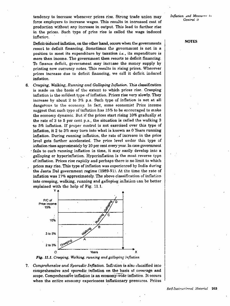
Inflation jnd Afeasuir*- in Control it
tendency to increase whenever prices rise. Strong trade union may force employers to increase wages. This results in increased cost of production without any increase in output. This lead to further rise in the prices. Such type of price rise is called the wage induced inflati.on.Deficit-induced inflation, on the other hand, occurs vdien the governments resoit to deflcit financing. Sometimes the govemmont is not in a position to meet its expenditure by taxation i.e., its expenditure is more than income. The government then resorts to deficit financing, lb finance deficit, government may increase the money supply by printing now currency notes. This results in rising prices. Wherever prices increase due to deficit financing, we call it deficit induced inflation.
6. Creeping. 'Walking, Running and Galloping Inflation. This classification is made on the basis of the extent to which prices rise. Creeping inflation is the mildest type of inflation. Prices rise very slowly. They increase by about 2 to 3% p.a. Such type of inflation is not at all dangerous to the economy. In fact, some economist Price income suggest that such type of inflation has 15% to be encouraged to make the economy dynamic. But if the prices start rising 10% gradually at the rate of 3 to 6 per cent p.a., the situation is called the walking 3 to 5% inflation. If proper control is not exercised over this type of inflation, it 2 to 3% may turn into what is known as 0 Years running inflation. During running inflation, the rate of increase in the price level gets further accelerated. The price level under this type of inflation rises approximately by 10 per cent every year. In case government
• fails to curb running inflation in time, it may easily develop into a galloping or hyperinflation. Hyperinflation is the most reverse type of inflation. Prices rise rapidly and perhaps there is no limit to which prices may rise. This type of inflation was experienced by India during the Janta Dal government regime (1989-Sl). At the time the rate of inflation was 17% approximately. The above classification of inflation into creeping, walking, running and galloping inflation can be better explained with the help of Fig. 11.1.
NOTES
V *
JP/C of
Price income 15%
D
C10%
B
3 to 5%
A
2 to 3%
XYearsFig. 11.1. Creeping. Walking, running and galloping inflation
7. Comprehensive and Sporadic Inflation. Infl.'tiion is atsu classified into comprehensive and sporadic inflation on the basis of coverage and scope. Comprehensive inflation is an economy-wide inflation. It occurs when the entire economy experiences inflationary pressures. Prices
0
Sflf-Instnicti'inai Material 203
Industrial Economy and Principles of Management
of all commodities rise in the economy. Price rise is not confined to any particular sector. It extends to every sector in the economy. It is normal inflationary phenomenon and refers to the rising prices of the general price level. Sporadic inflation on the other hand, is sectorial in nature. It refers to a situation wherein inflation is experienced by certain sector of the economy. It may occur on account of restricted supply of certain commodities due to certain specific reason like crop failure resulting in the price rise of foodgrains or formation of a successful monopoly in the manufacturing sector causing price rise only in the manufacturing sector.' Sporadic inflation is thus confined to only certain sectors in the economy.
NOTES
NATURE, FEATURES AND CHARACTERISTIC OF INFLATIONCharacteristics and features of inflation are as follows ;
Inflation is an economic phenomenon. It is the re.«ult of economic forces.Inflation is also a monetary phenomenon. Excess supply of money may cause inflation.Cyclical movement is not inflation.The hall mark of inflation is excess demand in relation to everything. Inflation is a dynamic process which can be observed only over a long period of time.It is always associated with an uninterrupted rise in prices.Price rise is persistent and irreversible immediately. It is different from temporary price rise.Pure inflation is a past full employment phenomenon.
1.
2.
3.4.5.
6.7.
8.
CAUSES OF INFLATIONInflation in an economy arise on .account of number of factors. These factors relate mainly either to the demand or to the supply side. By demand we mean the demand of money income for goods and services and by supply we imply the available output for which the money income can be spent. Expectation also play an important role in causing inflationary pressures in the country. Therefore, the factors that cause inflation may be divided into three groups :
1. Demand FactorsIncrease in demand may be due to :
Increase in disposable incomes.Increase in community’s aggregate spending on consumption and investment goods.Excessive speculation and tendency to hoarding and profiteering on the part of producers and traders.Increase in salaries, wages or dearness allowance.Increase in foreign demand and hence exports.
(a)(i)
(0
W)(e)
204 Self-Iketructional Material
if) Increase in population.ig) Incr<?ase in money supply.
These causes may operate singly or in combination with one another. Generally, the most important cause of inflation is excessive public expenditure financed by deficit financing during war or on the implementation of plans for economic development. The newly created money increases government demand for goods and services and also the purchasing power of the people through increase in disposable income.
Inflation and Measures to Contrhl it
NOTES
2. Supply F'actorsNo corresponding increase in the output of goods and services may be due to:
(a) Increase in exports for earning the required foreign exchange.(b) Draught, famine or any other natural calamity adversely affecting
agricultural production.(c) Deficiency of capital equipment.
fcO Scarcity of other complemenlar factors of production e.g., skilled labour or technicians, cssentio! raw materials or lack of dynamic entrepreneur.
(e) Speculative hoarding by the producers, traders and middlemen in anticipation of a further .rise ra prices.
if) Prolonged industrial unrest resulting in reduction of industrial production.
3. Role of Expectation
Inflation cannot be explained onlv in terms of excessive spending relative to available output. Expectations play an important role in the speed of inflation. Expectations regarding future movement of prices and wages result in the inflationary pressure in the economy. When prices are expected to increase, consumers will purchase more goods. This will lead to an increase in the price level. Similarly, a rise in the expected income induces people to spend more. Expected wage increase also bring about inflation in the country. Expectations thus play a vital role in causing inflation in .an economy.
EFFECTS OF INFLATIONInflation indicates the rise in the price level and a fall in the value of money, llie efiects of inflation can be broadly classified under following three categories.
1. Political Affects of Inflation. Inflation also leads to political upheavals. Political indiscipline grows and corrupt practices become common. Hitler became dictator of Germany only because of hyper-inflation during 1920s. Political revolutions are the outcome of inflationary rise in prices. Political and economic speculations are encouraged by inflation. Political stability is disturbed by inflation.
2. Econcnxic Effects of Inflation. Economic effects of inAation can be studied under following two heads :(o) Effects on distribution of income. Inflation redistributes income
. because prices of all factors do not rise in the same proportion. The effect of inflation on the incomes of different classes of earners is .not uniform. Following classes of people are affected by it ;
Self-tnst’-urf’onnI Mntenal 20?
' t-.
Industrial EcoiiortTy and Principles of MariiipemenI
{;). Working class. Wages do not rise as fast as the prices rise during inflation. Nntu?'a]ly, workers tend to lose during the period of
. rising prices. The trade unions try to bargain with their employers for higher wages. Still the rise in wages is not corresponding to a rise in the prices. So, the workers are adversely affected during inflation. Salaried people have a more harsh effect of inflation than the wage-eaners as they are not organised like the salaried people.
Hi) Consumers. Inflation reduces the consumption of people. Rising price reduces private consumption by reducing the purchasing power in the hands of the people. The resources left unused can be secured by the government by printing new currency notes 'or I’aising the public debt. Thus, inllation can transfer the resources from the public to the government. The reduced consumption of the public or increased savings is termed as the phenomenon of forced savings. Forced savings have been made use of by many countries for their economic development. However, consumers have to load a low standard of living in the initial stages of development.The effects of inflation have been nicely concluded by Kenneth K. Kurihara in the following manner ... "inflation redistributed wealth and income in such a ivay as to hurt consumers, creditors, small investors and low and fixed income group, and benefits businessmen. debtors and farmers.°
Hii) Renteir class. People whose incomes are fixed (the rentier class) viz, pensioners, annuity holders, people living on past savings, etc., suffer the most during inflation. Inflation causes the real income of these people to fall due to rising prices. Falling real income reduces their standard of living. Inflation is thus harmful to the rentier class.
(to) Debtors and creditors. Debtors as a group arc behefltted during inflation whereas the creditors are put to loss. The debts are always fixed in terms of money in the modern economy. When a person borrows money before rise in the price level and repays later when prices have risen, he pays back the same amount of money but definitely having loss purchasing power. Creditors are at a loss during inflation as they receive money having less purchasing power.
(c) Farmers. Farmers are benefitted during inflation because of two . factors:
(a) The price of farm products increase; and (6) increase in the cost of production lags behind the rise in the prices. Farmers who produce foodgrains and other highly inflation-sensitive products are benefitted the most. Farmers in debts repayment repay their old debts along with the rate of interest as they get profits due to rising prices. They are further benefitted as debtors as they pay back lower purchasing power to the creditors. Inflation thus provides double advantages to the farmers.
(ri) Business community. The manufacturers, merchants and entrepreneurs stand to gain during inflation. The value of stocks held by the merchants increases during inflation. Business
NOTES
20B Self-lnstructionnl Mnrcrial
Inflation and A^easH/•e^• to Control il
community sells commodities at bettor prices and eai-n high profits. Enterpreneurs earn huge profits as the rise in the price will be more than the rise in the cost of production. Producers try to increase the price in the cost of production instead of reducing their margin of profits. Inflation has favourable effect on the business community.
iuii) Investors. Inflation is favourable to those who invest in equities, but is rather harsh to those who invest in fixed interest yielding bonds. Equity dividends increase during inflation due to increased corporate earnings and investors in equities are benefitted. Fixed interest yielding bonds bring the same income but less purchasing power. Institutional investors safeguard their interest by diversifying their resources in profitable investments, hut small and middle class investors lose much. In many countries small investors have experienced heavy losses because of the fall in the purchasing, power of money. The fall in the value of money discourages saving and therefore, reduces the volume of funds available for investment in a free market economy.
ib) Effects on production. Keynes is of the opinion that a moderate rise in prices i.e., mild or creeping inflation has a favourable effect on production when there are utilised or underemployed resources in existence in an economy. Such a rise in prices creates optimism among the business community as they get more profits with increasing prices. They arfe induced to invest more and as a result employment, output and income will increase. The limit is set by the full employment, level. Once the full employment stage is- reached in the economy a further rise in tlie price will not stimulate production, empioj'ment and income due to physical limitations. So, till the level of full employment is reached, moderately rising prices are beneficial. The beneficial effect.s on pioduttioh are possible only when inflation is moderate. A state of running or galloping inflation creates a lot of uncertainty which is harmful to production;
3. Social Effects of Inflation. Inflation not only creates economic effects but also loads to certain social effects. It brings down the standards of business morality by encouraging a few rich pci'sons. Black-marketing, anti-social activities dominate the society during inflationary rise in prices. Social peace is disturbed. Frustration exists among poor people. This likely result in a social revolt. Social atmosphere gets totally spoiled as rich men try to exploit the situation and take undue advantage of inflation. Social stability is at stake. Unfair practices and social discontent become order of the day. Patriotic people are penalised.
NOTES
CONTROL OF INFLATIONInflation is very complex phenomenon. There is no one sovereign remedy to combat it. On the other hand, measures have to be taken on several fronts, monetary and non-monetary, to fight it. All these measures have one common aim. They aim at reducing aggregate monetary expenditure taking the available output as given. Broadly speaking, the anti-inflationary measures can be classified as under:
Self-Intitriictional Material 20"
Industrial Economy and Principles of Management 1. Monetary Measures. According to some economists, inflation is a
monetary phenomenon, t.e., it is caused by the monetary factors. These economists suggest that the control over the supply of money is the best measure to combat inflation.The anti-inflationary monetary policy refers to the central banking operations of restricting credit. The Reserve Bank of India makes use of its weapons like the bank-rate policy, open market operations, variable reserve ratio and the selective credit controls to restrict credit. The monetary policy can successfully control inflation only when it is caused by the excess supply of money.
2. Fiscal Measures. The two wings of fiscal policy are government revenues and gf!\’enimnnt expenditure. The government’s fiscal policy can contribute to the control of inflation either expenditure, but decreasing government expenditrue or combining both the elements. If private spending tends to excessive, the government can moderate the inflationary pressure by reducing its own reduction or postponement of government expenditure in modern times is not an easy task. There may be projects already under construction and these obviously cannot be postponed. Similarly other types of expenditure may be necessary to meet the normal requirements of the ‘collective consumption’ of the community-defence, police, justice etc. Then, their may be social expenditures on education, health etc., which are very difficult to cut because of undesirable political effects. Therefore, the major emphasis of fiscal policy in inflation Has been a reducing private spending through increased taxation.An increase in taxes tends to reduce private spending. If the rates of direct taxes on incomes and profits are raised, the private disposable income is reduced and this will tend to reduce private consumption spending. If the rate of commodity taxes are increased or fresh levies are made, the effect on consumption will be more immediate. An increase in the tax rales on a commodity will penalise spending directly by raising the cost of purchases.Thus in period of inflation, the government should curb its own spending and increase the tax rates to reduce private spending. It is good thing to plan for a budget surplus during inflationary periods.
3. Other Measures. There are also other physical measures to control inflation. For instance, government may try to increase output and thereby control inflation.. In countries, like India where inflation is because of the shortage of agricultural commodities, it can be controlled by increasing the output of agricultural commodities. E\’en in developed countries, by changing the techniques of production, the level of full employment output can itself be increased and be adjusted to the increased aggregate demand. There may be physical restraints on the increase in output and, therefore, we h.iTe to note the problems • of technique, availability of factors of production in increasing output. Inflation may also be due to the speculation activities, business expectations and hoardings. Under such circumstances, the government may try to restrict speculativ’e activities to control inflation. In India, in order to protect the consumers from the evils of speculative activities, the government of India has given greater importance for the distribution of essential commodities through consumers’ co-operatives.
NOTES
208 Silf-Instructional Material
Inflation and Measurts to Control it
If the rise in the price confined only to some commodities the government may try to control their prices through price controls and rationing of the scare commodities. Rationing and price controls suffer from a severe limitation viz-, coercion cannot be extensively made use of in a democratic country.Lastly, if the inflation is due to the increase in cost (cost-push inflation), it can be controlled by wage freeze. The Government may try to put
. an end to the wage price spiral by freezing wages. This policy becomes effective if the trade unions do not object to the control over wages. Further, if the government wants to control, wages, prices should not be allowed to rise, so that the standard of living of the consumers is not adversely affected.
NOTES
Self-Instructional Materidl 209
industrial Economy and Principles of Mdrtagement
STUDENT ACTIVITY
1. Define .inflation and discuss its effects. How far can monetary measures control inflation ?
2. Indicate the effect of a rise in the level of price on (a) wage earners (b) businessmen and (c) persons with fixed income.
210 Self-Instructional Material
Inflation and Measures to Control itSUMMARY
A rise in price level or fall in the value of money is often the result of the excessive amount of money, or excessive issue of paper currency and this is commonly referred to as inflation.The most important cause of inflation is excessive public expenditure financed by deficit financing during war or on the implementation of plans for economic development.Inflation indicates the rise in the price level and a fall in the value of money.
NOTES
REVIEW EXERCISESWhat are the causes of price inflation ?. Is it inevitable in the course of economic development ?“inflation is unjust and inequitable”. Discuss.Briefly enumerate the consequences of inflation on various classes. How far can monetary measures control inflation ?What do you understand by deflation ? Discuss its consequences. Elaborate the measures to control deflation.
1.
2.3.
4.
Self-Instructional Material 211
Industrial Economy and Principles of Management UNIT 12 BUSINESS FLUCTUATIONS
NOTES ★ STRUCTURE ★□ Introduction
□ Concept of Business (Trade) Cycle
□ Nature, Features and Characteristics of Business Cycle
□ Classification of Business Fluctuations
INTRODUCTIONThe records .of business activity world over indicate that the course of business is not smooth. Periodic fluctuations in business and economic activities at more or less regular intervals has been an important feature of all the capitalist economies. These fluctuations of business are of many kinds. Some are abrupt and discontinuous as caused by war. Some are continuous in the same direction, when steady economic growth takes place. Other changes are fluctuations of a rhythmic nature which get manifested in the form of expansion and contraction of business activity. These are commonly called “trade cycles” or "business cycles”. Business cycles are not limited to specific fields they tend to spread over the entire field of business activity. A trade cycle generally has a length of time varying from four to twelve years, while at certain times, trade cycles of twenty years length have also been witnessed. Normally, the duration of a trade cycle is of eight to nine years.
CONCEPT OF BUSINESS (TRADE) CYCLEA business cycle can be defined as wave like fluctuations of business activity characterised by recurring phase of expansion and cohtraction in periods varying from three to four years. This relatively simple definition of a business cycle suggests that business activity never takes place in a steady'manner. While the business makes progress overtime, there are also fluctuations in it. This implies that the period of business expansion comes to an end sooner or later. After the turning point the business activity passes through the phase of contraction which also terminates in a few years and once again the business activity finds itself on the expansion path."Business cycles are a type of fluctuations found in the aggregate economic activity of nations that organise their work mainly in business enterprises. A cycle consists of expansions occurring at about the same time in many economic activities followed by similarly general recessions. Contractions and revivals, which merge with the expansion phase of the next cycle. This sequence of change is recurrent but not periodic.”Mitchell’s definition states that business cycles are fluctuations in economic activity as a whole. Hence, they are to be distinguished from the fluctuations
—^Mitchell
212 Self-Instructional Material
Business Flucluationtwhich are limited to specific fields. Generally, because of sectoral linkage, fiuctuations in particular fields do not remain confined to those sectors only where they originate, It is commonly observed that a recession in consumer goods manufacturing sector causes recession in the capital goods sector as well. Not only this, a decline in industrial activity leads to a slump in overall economic activity. Therefore, the point of distinction between the fluctuations taking place in individual sectors and the fiuctuations in the aggregate economic activity should not be overstressed.
NOTES
.-ATURE, FEATURES AND CHARACTERISTICS OF BUSINESS CYCLEFeatures and characteristics of a business cycle are as follows :
1. Business cycle is characterised by fluctuations which occur periodically in a free rhythm. This implies that the recurrence of expansion and contraction has no fixed or invariable period.
2. A typical business cycle completes itself in a period of 3 to 4 years. In some cases, duration of business cycle is shorter or longer than those of normal business cycle. In any case, the period of business cycle is not shorter than one year. A business cycle in its character is distinctly different from fluctuations in economic activity which take place within the period of calender year and are due to causes connected directly or indirectly with the physical season.
3. A business cycle is characterised by alternating forces leading an economy to prosperity and depression. These forces are in built-in the system, The force of expansion when bom, gathers momentum over-time taking the economy to a high level of activity. This force is, however, first weakend and then completely replaced by a counter force which leads to contraction and the process ends up with depression.
4. According to Keynes, an important characteristics of the business cycle is the phenomenon of crisis. This implies that the peak and the through are asymmetrical. Normally the prosperity phase of business cycle comes to an end abruptly, whereas recovery after the depression is gradual and slow.
Phases of Business CycleNo business cycle is same as another. In other words, the details of cycles differ. However, all the cycles belong to the same family and thus have common characteristics. According to the Burus and Mitchell, every business cycle has the critical mark
■ off points of peak and trough. From trough to peak there is the expansion phase and from peak to trough the contraction phase. Apart from these two relatively longer phases these are two other phases characterised by the turning points. The upper turning point located at the peak marks the beginning of recession, while the other turning point located at the trough is the venue of revival. Both recession and revival phases are relatively short in duration.In general, the various phases of trade cycle can be stated as follows. (Fig. 12:1,)
1. Prosperity •3. Depression
2. Recession 4. Recovery.
Self-Instructional Material 31?
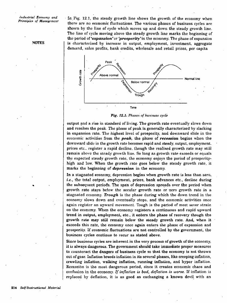
■indiintrial Eamomy and PrintipUn of Management In Fig. 12.1, the steady growth line shows the growth of the economy when
there are no economic fluctuations. The various phases of business cycles are shown by the line of cycle which moves up and down the steady growth line. The line of cycle moving above the steady growth line marks the beginning of the period of‘expansion'ar ‘prosperity’in the economy. The phase of expansion is characterised by increase in output, employment, investment, aggregate demand, sales profits, bank credits, wholesale and retail prices, per capita
NOTES
Peak\
// %2 Above normalI Normal line7g Below normalO
%Trough
Time
Tig. 12.li Phases of business cycle
output and a rise in standard of living. The growth rate eventually slows down and reaches the peak. The phase of peak is generally characterised by slacking in expansion rate. The highest level of prosperity, and downward slide in the economic activities from the peak, the phase of recession begins when the downward slide in the growth rate becomes rapid and steady, output, employment, prices etc., register a rapid decline, though the realised growi;h rate may still remain above the steady growth line. So long as growth rate exceeds or equals the expected steady growth rate, the economy enjoys the period of prosperity- high and low. When the giowth rate goes below the steady growth rate, it marks the beginning of depression in the economy.In a stagnated economy, depression begins when growth rate is less than zero, t.e., the total output, employment, prices, bank advances etc., decline during the subsequent periods. The span of depression spreads over the period when growth rate stays below the secular growth rate or zero growth rate in a stagnated economy. Trough is the phase during which the down trend in the economy slows down and eventually stops, and the economic activities once again regi.ster an upward movement. Tough is the period of most sever strain on the economy. When the economy registers a continuous and rapid upward trend in output, employment, etc., it eaters .the phase of recovery though the growth rate may still remain below the steady growth rate. And, when it exceeds this rate, the economy once again enters the phase of expansion and prosperity. If economic fluctuations are not controlled by the government, the business cycles continue to recur as stated above.Since business cycles are inherent in the very process of growth of the economy, it is always dangerous. The government should take immediate proper measures to counteract the dangers of business cycle so that the economy is not thrown out of gear. Inflation breeds inflation in its several phases, like creeping inflation, crawling inflation, walking inflation, running inflation, and hyper inflation. Recession is the most dangerous period, since it creates economic chaos and confusion in the economy. If inflation is bad, deflation is worse. If inflation is replaced by deflation, it is as good as exchanging a known devil with an
214 Self-Instructional Material
Business Fluctualioiisunknown devil. During the period of hectic inflation, consumers go to the market with bags full of money, and return home with pockets full of commodities and this is because of rocketing prices in the market. Deflation is a very bad period of economic dislocation and distortions. Though prices are very low, people will have very little purchasing power. Due to the absence of profits during deflation, the investors will have no incentives or inducements to make investments. Thus, both the periods are dangerous and it will be the responsibility of the government to take steps to prevent the occurrence of these economic fluctuations.
NOTES
CLASSIFICATION OF BUSINESS FLUCTUATIONSThe most common classification of business fluctuations are as follows :
Seasonal Trends. Seasonal fluctuations refer to the periodic movements in business activity that take place due to changing seasons within the period of a calender year. These fluctuations are observed in various business and economic phenomenon like prices of industrial products, agricultural commodities, bank clearings, interest rates etc. Social customs are also the causes for seasonal variations in economic activities. Seasonal variations do not present any serious sociai or economic problems, since they are predictable well in advance.Secular Trends. A persistent movement continuing in the same direction over a long period of time is called secular trend. A long period of secular trend generally encompasses within it a number of business cycles. In the study of economic fluctuations and business forecasting, secular trends are the best, since they have an impact on long-term forces making for change. In the total economy, secular movements reflect changes in population growth, technology, accumulation of capital, propensity to consumer and saving which cause changes over a long-term.Random Trends. The random trends are noo-recurring and irregular,. operating in the economy in bringing about revolutionary and sporadic changes. Floods, earthtluakes, storms, famines, strikes, tomedos etc., are very good examples. Most of these factors are accidental in character. They are unpredictable, non-mcasurable and non-periodic. All these trends are inteirelated and interwoven. Cyclical fluctuations have attracted major attention of the economists, since their impact is very severe.Cyclical TYends. Economic activity moves continuously throiigh altematicms of rise and fall and they are called cyclical fluctuations, which are wave like fluctuations of economic activity characterised by recurring phases of expansion and contractions. Cycles are rhythmic and irregular, but they have stipulated pattern, but difficult to predict.
1.
2.
3.
4.
Self-Instruclional Material 215
Industrial Ecoiiomy and Principles of Management
STUDENT ACTIVITY
1. ‘Btisiness fluctuations are manifested in the form of expansion and contraction of business activity”. Explain the statement.
2. What are the different phases of a business fluctuations ?
216 Stlf-In»tructionai Material
Busines$ FluctuationsSUMMARY I
• Periodic fluctuations in business and economic activities at more or less regular intervals has been an important feature of all the capitalist
• economies.• A business cycle can be defined as wave like fluctuations of business activity
characterised by recurring phase of expansion and contraction in periods varying from three to four years.
• Business cycle is characterised by fluctuations which occur periodically in a free rhythm. This impbes that the recurrence of expansion and contraction has no fixed or invariable period.
INOTES
REVIEW EXERCISES1. Explain the features and characteristics of a business cycle.2. Explain the classification of business fluctuations.
''s.
Self-Instructional Material 217