Security Analysts and Capital Market Anomalies

Li Guo a, Frank Weikai Li b, and K.C. John Wei c

a Singapore Management University, Lee Kong Chian School of Business

Singapore, Email: liguo.2014@pbs.smu.edu.sg

b Singapore Management University, Lee Kong Chian School of Business

Singapore, Email: wkli@smu.edu.sg

c School of Accounting and Finance, Hong Kong Polytech University

Hung Hom, Hong Kong, Email: johnwei@ust.hk

This Draft: August 2018

_____________________________________________________________________________

Abstract

We examine whether analysts use information in well-known stock return anomalies when

making recommendations. We find results contrary to the common view that analysts are

sophisticated information intermediaries who help improve market efficiency. Specifically, when

analysts make more favorable recommendations to stocks classified as overvalued, these stocks

tend to have particularly large negative abnormal returns ex post. Moreover, analysts whose

recommendations are more aligned with anomaly signals are more skilled and elicit greater

recommendation announcement returns. Our results suggest that analysts’ biased

recommendations could be a source of market frictions that impede the efficient correction of

mispricing.

JEL classification: G12, G14

Keywords: Analysts; Analyst recommendation; Mispricing; Market efficiency

We thank Utpal Bhattacharya, Claire Yurong Hong, Gang Hu, Roger Loh, James Ohlson, Baolian Wang, Aaron

Yoon (MIT Asia discussant), Chishen Wei, Jialin Yu, and seminar and conference participants at Hong Kong

Polytech University, National Chengchi University, National Sun Yat-sen University, National Taiwan University,

Singapore Management University, and the 2018 MIT Asia Conference in Accounting (MIT Asia) for their helpful

comments and suggestions. John Wei acknowledges financial support from the Research Grants Council of the

Hong Kong Special Administrative Region, China (GRF15503517). All remaining errors are our own.

Corresponding author: K.C. John Wei, School of Accounting and Finance, Hong Kong Polytechnic University,

Hung Hom, Kowloon, Hong Kong. E-mail: johnwei@ust.hk; Tel: 852-2766-4953; Fax: 852-2330-9845.

Security Analysts and Capital Market Anomalies

Abstract

We examine whether analysts use information in well-known stock return anomalies when

making recommendations. We find results contrary to the common view that analysts are

sophisticated information intermediaries who help improve market efficiency. Specifically, when

analysts make more favorable recommendations to stocks classified as overvalued, these stocks

tend to have particularly large negative abnormal returns ex post. Moreover, analysts whose

recommendations are more aligned with anomaly signals are more skilled and elicit greater

recommendation announcement returns. Our results suggest that analysts’ biased

recommendations could be a source of market frictions that impede the efficient correction of

mispricing.

JEL classification: G12, G14

Keywords: Analysts; Analyst recommendation; Mispricing; Market efficiency

1

“Wall Street analysts know their companies. You should cut a research report in two. The first

part, the information about the company and its prospects, is probably pretty good. The second

part, the recommendation, should be used as kindling. We use analyst information, but we don’t

use the recommendations very often.” David Dreman

1. Introduction

A long-standing debate in the finance and accounting literature concerns whether security

analysts’ research helps to improve stock market efficiency. Early studies that examine market

reactions to analyst earnings forecast revisions or recommendation changes tend to support the

notion that analysts are skilled information processors (Womack, 1996; Barber et al., 2001).

Analysts’ information-production role helps to improve price efficiency. However, recent studies

question the usefulness of analyst research outputs, arguing that analysts’ incentives to gain

investment-banking business, to generate trading commissions, or to curry favor with

management for access to private information compromise their integrity and objectivity (Lin

and McNichols, 1998; Chen and Matsumoto, 2006; Cowen, Groysberg, and Healy, 2006). More

generally, Bradshaw, Richardson, and Sloan (2006) find that a firm’s level of external financing

is a more important driver of analyst optimism than existing investment banking ties. This

suggests that even unaffiliated analysts may upwardly bias their forecasts or recommendations in

anticipation of future business. In addition to conflicts of interest arising from investment

banking/brokerage affiliations, analyst recommendations or forecasts may be biased for non-

strategic reasons (La Porta, 1996).

In this paper, we address this important question by examining whether analysts exploit

well-documented stock return anomalies when making recommendations. Over the past several

decades, researchers have discovered numerous cross-sectional stock return anomalies.

Irrespective of the sources of return predictability, these anomalies represent publically available

information, of which skilled agents, such as analysts, should be able to take advantage. If

2

analysts are truly sophisticated, informed, and unbiased, they should exploit such well-known

sources of return predictability when making recommendations.1

We propose two competing views on analyst research that offer opposite predictions to our

research question. The sophisticated analyst hypothesis predicts that analysts should on average

tilt their recommendations to be consistent with anomaly prescriptions. In contrast, the biased

analyst hypothesis suggests that analyst recommendations are unrelated or even contradictory to

anomaly prescriptions. More importantly, the two competing hypotheses have different asset

pricing implications when analyst recommendations disagree with anomaly prescriptions. The

sophisticated analyst hypothesis predicts that when analyst recommendations contradict anomaly

prescriptions, anomaly stocks should not be associated with future abnormal returns. In sharp

contrast, the biased analyst hypothesis predicts that anomaly returns can be amplified when

analysts disagree with anomaly prescriptions, especially if certain groups of investors naïvely or

strategically follow analyst recommendations.2 In other words, biased analyst recommendations

are a potential source of market frictions that contribute to sustained mispricing.

Following Stambaugh, Yu, and Yuan (2012; 2015), we construct 11 prominent asset

pricing anomalies using the sample with available analyst recommendation data from the

Institutional Brokers’ Estimate System (I/B/E/S). We first show that during our sample period of

1993-2014, all long-short portfolios based on these 11 anomalies generate significant Fama and

French (1993) three-factor alphas, ranging from 0.35% to 1.09% per month. Following

Stambaugh and Yuan (2017), we also create two composite mispricing scores, MGMT and

1 We focus on analyst recommendations because they directly reflect analysts’ view of the relative over- or under-

valuation of a stock, while analysts’ forecasts of firm earnings do not directly correspond to their perception of

relative misvaluation. 2 Mikhail, Walther, and Willis (2007) and Malmendier and Shanthikumar (2007) find that small investors naïvely

follow analyst recommendations, without accounting for analysts’ biased incentives. Brown, Wei, and Wermers

(2014) show that mutual funds tend to herd into with consensus sell-side analyst upgrades, and herd out of stocks

with consensus downgrades, and that herding by career-concerned fund managers is price destabilizing.

3

PERF, which generate monthly three-factor alphas of 0.86% and 0.99%, respectively.3 This

strong return predictability suggests that anomaly signals should be part of the information set

that analysts can use when making their stock recommendations.

To examine whether analysts incorporate anomaly signals into their recommendation

decisions, we analyze the level and change of analyst recommendations during the window of

anomaly portfolio formation.4 The results strongly reject the sophisticated analyst hypothesis.

First, not only do analysts fail to tilt their recommendations to take advantage of anomalies, but

also their recommendations are often contradictory to anomaly predictions. This tendency is

particularly strong for anomalies related to equity issuance and investment. For example, for

MGMT, the mean recommendation value is 4.09 for stocks in the short leg and 3.53 for stocks in

the long leg with a difference of -0.56, which is highly significant. By contrast, analyst

recommendations seem to be more consistent with the prescriptions of the anomalies associated

with firm performance (PERF), such as gross profitability and return on assets, although the

relation is weak and not monotonic. The results are similar for recommendation changes, which

is particularly puzzling. It suggests that analysts are actively revising opinions on anomaly stocks,

but their views tend to be in the wrong direction of anomaly predictions. Thus, analyst

inattention or stale recommendation story cannot fully explain our findings.

The differential analyst behavior across the two categories of anomalies is consistent with

previous literature that finds that analysts tend to issue overly optimistic growth forecasts or

recommendations for firms characterized with high growth, large capital spending, and equity

financing needs. These firms are more likely to be potential investment banking clients of the

3 MGMT mainly consists of anomalies related to managerial actions, and PERF mainly consists of anomalies related

to firm performance. 4 We measure the change of recommendations by taking the difference between the current consensus

recommendation and its value one year ago.

4

brokerage firms employing the analysts. Analysts are also likely to issue more favorable

recommendations for better performing firms with high profitability or past winners.

However, analyst recommendation behavior itself is not sufficient to distinguish between

the two competing hypotheses. Analysts may have superior (private) information such that even

when their recommendations contradict anomaly prescriptions, the information value of their

recommendations can offset that of anomalies. We therefore examine anomaly returns when

analyst recommendations confirm or contradict anomaly signals. The result reveals the same

message. When analyst recommendations and anomaly prescriptions contradict, anomaly returns

are amplified, especially for the anomalies associated with PERF. The abnormal returns in

inconsistent cases are larger than those in consistent cases for all 11 anomalies, and significantly

so for 7 anomalies. For example, the long-short portfolio based on PERF generates a monthly

three-factor alpha of 1.57% for the inconsistent case, whereas it is only 0.90% for the consistent

case. The result is more pronounced in the short leg of anomalies with favorable

recommendations, which earns a particularly large negative return. This is consistent with the

idea that short selling overvalued stocks is costlier than correcting underpriced stocks (Nagel,

2005; Stambaugh et al., 2015), especially when betting against analyst consensus. The

amplification effect of analyst recommendations on anomalies is not driven by other firm

characteristics. The result from Fama and MacBeth (1973) regressions is similar, as we also

control for standard return predictors.

The preceding finding may mask heterogeneity across individual analysts who differ

significantly in their skills and incentives to generate informative recommendations. To shed

light on this issue, for each analyst we calculate the correlation between her recommendation

values and the two composite mispricing scores among all of the stocks covered by the analyst

5

during the past three years. Consistent with the idea that this correlation metric captures analysts’

skill or unbiasedness, we find that analysts with a higher correlation metric elicit stronger market

reactions when announcing recommendation changes.

We conduct several tests to rule out alternative explanations. First, analysts may simply be

unaware of the return predictability of these anomalies before their discoveries by academics

(McLean and Pontiff, 2016). However, we find that analysts’ tendency to recommend

overvalued stocks more favorably is still significant for six anomalies in the post-publication

period, suggesting that analysts’ unawareness of expected return information in the anomalies is

unlikely to fully explain our findings. Second, analysts can be reluctant to incorporate anomaly

signals into their recommendations as their institutional clients can face severe constraints when

trading these stocks. Using firm size and bid-ask spread as proxies for trading frictions, we find

very similar results for big or highly liquid stocks, suggesting that limits-to-arbitrage concerns on

the part of analysts is unlikely to explain our findings. Third, analyst recommendations can be

strategically biased to cater to institutional investors’ preferences for overvalued stocks (Edelen,

Ince, and Kadlec, 2016). However, we find very similar results for stocks partitioned by

institutional ownership, suggesting that the catering incentive cannot fully explain our findings.

Analyst recommendations can be biased due to misaligned incentive or behavioral bias.

Based on the Baker-Wurgler (2006) Sentiment Index, we find that analyst recommendations are

more biased toward overvalued stocks and that the amplification effect of biased

recommendations on anomaly returns is more pronounced during high- rather than low-

sentiment periods. This evidence suggests that the behavioral bias of analysts may partially

explain their overly optimistic (pessimistic) recommendations for overvalued (undervalued)

stocks.

6

Using analyst data from Zacks over an earlier sample period, Barber et al. (2001) and

Jegadeesh et al. (2004) document the investment value of both the level and change of analyst

consensus recommendations. To reconcile their evidence with our finding that analyst consensus

recommendations are on average inefficient, we re-examine the unconditional return

predictability of analyst consensus recommendations. Using I/B/E/S data over the sample period

from 1993 to 2014, we do not find any return predictability for the level of analyst consensus

recommendations. While we do find some return predictability for the change of consensus

recommendations over the full sample period, it is concentrated only in the 1993-2000 period.

Overall, we conclude that the seemingly contradictory results of our paper with those of prior

studies are mainly attributable to the different sample periods studied by these papers.

In a recent concurrent working paper, Engelberg, McLean, and Pontiff (2018b) document

similar evidence that analysts’ price forecasts and recommendations often contradict anomaly

predictions. Our paper differs from theirs by further showing that anomaly returns are

significantly amplified when analyst opinions contradict anomaly signals. We thus provide

stronger evidence that analysts’ biased recommendations contribute to the persistence of

anomalies. Moreover, we develop a simple method to identify skilled analysts ex ante.

2. Related Literature

2.1. Cross-sectional asset-pricing anomalies

Many stock return anomalies have been discovered over the last 40 years. Although the

sources of return predictability of these anomalies are under debate, the large abnormal returns

generated by some of these anomalies are well established. In this subsection, we start with the

7

11 prominent anomalies extensively examined by Stambaugh et al. (2012; 2015) to shed light on

the inference of analyst behavior and return anomalies.

Stambaugh and Yuan (2017) further propose two mispricing factors that are constructed

from these 11 prominent anomalies. They begin by separating the 11 anomalies into 2 clusters

based on the similarity in time-series anomaly returns and cross-sectional anomaly rankings. The

first cluster consists of six anomalies: net stock issuance (NSI), composite equity issuance (CEI),

accruals (Accrual), net operating assets (NOA), asset growth (AG), and investment to assets

(I/A). The authors find that these variables are most likely to be directly affected by the decisions

of firm managers. Therefore, the average ranking score based on these six anomalies reflects the

commonality of mispricing caused by firm managers’ decisions. The authors name the pricing

factor arising from this average ranking score as MGMT. The second cluster of anomalies

includes gross profitability (GP), return on assets (ROA), momentum (MOM), distress (Distress),

and O-score. These five anomaly variables are more related to firm performance and less directly

controlled by management. Stambaugh and Yuan (2017) denote the pricing factor generated

from this cluster as PERF. We describe each anomaly in detail as follows:

Cluster I anomalies (MGMT):

(1) Net stock issuance (NSI): Ritter (1991), Loughran and Ritter (1995), and Pontiff and

Woodgate (2008) find that firms issuing new shares underperform the market in the

following three to five years. Net stock issuance is calculated as the growth rate of the

split-adjusted shares outstanding in the previous year.

(2) Composite net equity issuance (CEI): Daniel and Titman (2006) and Fama and French

(2008) find that firms with higher composite net equity issues earn lower future risk-

adjusted returns. The composite net equity issuance includes any actions that increase

8

share issuance (such as seasoned equity offerings and share-based acquisitions) minus

any actions that reduce share issuance (such as share repurchases).

(3) Accounting accruals (Accrual): Sloan (1996) documents that firms with high total

accounting accruals subsequently earn lower risk-adjusted returns.

(4) Net operating assets (NOA): Hirshleifer, Hou, Teoh, and Zhang (2004) show that firms

with higher net operating assets subsequently earn lower risk-adjusted returns.

(5) Asset growth (AG): Cooper, Gulen, and Schill (2008) and Titman, Wei, and Xie (2013)

report that firms with higher growth in total assets subsequently earn lower risk-adjusted

returns.

(6) Investment to assets (I/A): Titman, Wei, and Xie (2004) and Xing (2008) find that firms

with higher past investment earn lower future risk-adjusted returns.

Cluster II anomalies (PERF):

(7) Gross profitability (GP): Novy-Marx (2012) and Chen, Sun, Wei, and Xie (2018) show

that firms with higher gross profits to assets earn higher risk-adjusted returns. Novy-Marx

argues that gross profitability is the cleanest measure of true economic profitability due to

low accounting manipulations.

(8) Return on assets (ROA): Fama and French (2006), Hou, Xue, and Zhang (2015), and

Chen, Sun, Wei, and Xie (2018) find that firms with higher profitability or higher return

on assets subsequently earn higher risk-adjusted returns.

(9) Medium-term momentum (MOM): Jegadeesh and Titman (1993) find that firms

performing well in the past 3-12 months continue to perform well in the next 3-12 months.

They further find that the strategy based on the past six-month returns, skipping one

month and holding for the next six months, is the most profitable.

9

(10) Financial distress 1 (Distress): Rational theory predicts that firms with higher financial

distress risk should earn higher returns to compensate for the risk. However, Campbell,

Hilscher, and Szilagyi (2008) and others find that firms with higher bankruptcy

probability earn lower risk-adjusted returns. The bankruptcy probability is estimated from

a dynamic logit model based on both accounting and equity market information.

(11) Financial distress 2 (O-score): Campbell et al. (2008) and others find that using the

Ohlson (1980) O-score as the distress measure produces similar results. The O-score is

estimated from a static model using accounting data alone.

In addition, several recent studies have examined an increasingly larger set of anomalies to

shed further light on the sources of cross-sectional return predictability. Harvey, Liu, and Zhu

(2016) develop a multiple hypothesis-testing framework and apply it to more than 300 factors.

They conclude that most of the anomalies or factors discovered previously are probably false.

Green, Hand, and Zhang (2017) find that only a small set of characteristics out of 94 are reliably

independent determinants of cross-sectional expected returns in non-microcap stocks, and return

predictability sharply fell after 2003. Similarly, McLean and Pontiff (2016) find that the return

predictability of 97 variables shown to predict cross-sectional stock returns declined significantly

post-publications, suggesting that investors learn about mispricing from academic studies.

However, Yan and Zheng (2017) evaluate 18,000 fundamental signals from financial statements,

show that many signals are significant predictors of cross-sectional stock returns even after

accounting for data mining, and suggest that anomalies are better explained by mispricing.

Engelberg, McLean, Pontiff (2018a) document that anomaly returns are many times higher on

news dates, suggesting that anomalies are the result of investors’ biased beliefs that are partially

corrected by the arrival of information. All of these large-scale anomaly studies contribute to our

10

understanding of whether the abnormal returns documented in previous studies are compensation

for systematic risks, evidence of market inefficiency, or simply the result of extensive data

mining.

2.2. Usefulness and biases of analyst research

Analysts are prominent information intermediaries in capital markets. They engage in

private information acquisition, perform prospective analyses aimed at forecasting a firm’s future

earnings and cash flows, and conduct retrospective analyses that interpret past events. Regulators

and other market participants view analysts’ activities and competition between them as

enhancing the informational efficiency of security prices. The importance of analysts’ role in

capital markets has spurred research showing that analysts influence the informational efficiency

of capital markets.

A long-standing question in the finance and accounting literature examines whether

security analysts’ research is useful for market participants. Early studies using short-run event

windows to measure market reactions usually find that analyst forecasts and recommendation

changes illicit large announcement returns. Elton, Gruber, and Grossman (1986) and Womack

(1996) show that firms that receive buy (sell) recommendations tend to earn higher (lower)

abnormal returns in the subsequent one to six months. Barber et al. (2001) extend the

investigation to consensus recommendations. They document the potential to earn higher returns

by buying the most highly recommended stocks and short selling the least favorably

recommended stocks. Jegadeesh et al. (2004) find that the level of consensus recommendation

adds value only to stocks with favorable quantitative characteristics and that the change in

consensus recommendations is a more robust return predictor.

11

However, recent studies have shown that analysts’ employment incentives create

predictable biases in their research outputs and coverage decisions.5 For example, McNichols

and O’Brien (1997) report that the distribution of analysts’ buy/sell recommendations is

positively skewed because analysts are averse to conveying negative signals. La Porta (1996)

finds that analysts over-extrapolate past growth trends and that their forecasts of long-term

growth rates negatively predict stock returns, which contributes to the value premium. Jegadeesh

et al. (2004) provide evidence that analyst recommendations are positively associated with some

accounting, valuation, and growth characteristics that are negatively associated with future

returns.

Drake, Rees, and Swanson (2011) find that short sellers often trade against analyst

recommendations and that these trades are highly profitable. Analyst incentives to misinform,

combined with mounting evidence of market inefficiency with respect to analyst reports (i.e., the

market’s fixation or under- or over-reactions to analyst reports), imply that analyst research

cannot be unambiguously interpreted as serving to enhance the informational efficiency of

capital markets. Specifically, analysts employed by brokerage houses that are affiliated with

covered firms through an underwriting relationship issue more optimistic recommendations,

earnings forecasts, and long-term growth forecasts than do unaffiliated analysts.6 They are also

less likely to reveal negative news.7

Finally, several recent studies have argued that the number of analysts covering a firm is an

informative signal for future firm fundamentals and stock returns (Das, Guo, and Zhang, 2006;

Jung, Wong, and Zhang, 2014; Lee and So, 2017). A typical security analyst faces non-trivial

5 See, for example, Womack (1996), Bradshaw (2004), and Groysberg, Healy, and Maber (2011). 6 See, for example, Dugar and Nathan (1995), Lin and McNichols (1998), and Dechow, Hutton, and Sloan (2000). 7 See, for example, O’Brien, McNichols, and Lin (2005).

12

switching costs when making coverage decisions. Given their incentive structure, analysts’

choices of which firms to cover should reflect their true expectation of firms’ future performance.

2.3. Market participants and capital market anomalies

The existence and persistence of well-documented stock return anomalies have spurred a

growing interest in investigating the underlying causes. Several recent papers argue that

institutional investors and mutual funds in particular, through their correlated trading behavior,

may contribute to the pervasiveness of these anomaly patterns. Jiang (2010) argues that herding

among institutional investors contributes to the value effect. Edelen, Ince, and Kadlec (2016)

find that institutional investors tend to trade contrary to anomaly prescriptions and that their

trading amplifies anomaly returns. Akbas et al. (2015) find that aggregate flows into the mutual

fund sector exacerbates well-known stock return anomalies, while aggregate flows into the hedge

fund sector attenuate anomalies.

With the tremendous growth of the hedge fund sector in the recent decade, studies have

begun to examine the relation between the trading behavior of these sophisticated investors and

anomalies. Using short interest as a proxy for arbitrage capital, Hanson and Sunderam (2014)

find that an increase in arbitrage capital on the anomalies has resulted in lower strategy returns.

Chen, Da, and Huang (2018) propose a measure of net arbitrage trading based on the difference

between abnormal hedge fund holdings and abnormal short interests on a stock. They find that

anomaly returns come exclusively from the stocks traded by arbitrageurs. Anginer, Hoberg, and

Seyhun (2015) show that the return predictability of anomalies disappears when insider trading

disagrees with the anomalies.

13

3. Data and Summary Statistics

Analyst consensus recommendations data come from the I/B/E/S summary file, while the

individual analyst recommendations are from the I/B/E/S detail history file. The I/B/E/S detailed

recommendation data begin in December 1992 and consensus recommendations start from 1993.

Recommendation value is coded as a number from 5 (strong buy) to 1 (strong sell). We also

construct the change of consensus recommendations (∆𝑅𝑒𝑐), as Jegadeesh et al. (2004) find that

recommendation changes are more informative than recommendation levels. The

recommendation change is calculated as the current consensus recommendation minus its value

on the same firm one year ago. We merge the analyst data with the Center for Research in

Security Prices (CRSP) data after eliminating firms with share codes other than 10 or 11 and

firms with stock prices below $1.

Following Stambaugh and Yuan (2017), anomaly measures are constructed at the end of

each month t. For the anomaly variables requiring annual financial statements from Compustat,

we require at least a four-month gap between the portfolio formation month and the end of the

fiscal year. For the quarterly reported earnings, we use the most recent data in which the earnings

announcement date (RDQ in Compustat) precedes month t. For the quarterly balance sheet items,

we use the data from the prior quarter.

We construct anomaly portfolios as follows. We sort all of the stocks into quintile

portfolios based on each of the anomaly characteristics at the end of each month, and define the

long- and short legs as the extreme quintiles. When constructing the composite mispricing

factors, we require a stock to have a non-missing value at the end of month t - 1 for at least three

of the anomalies to be included in that composite mispricing measure. For an anomaly to be

14

included in the composite mispricing measure at the end of month t - 1, we also require at least

30 stocks to have non-missing values for that anomaly.

We also calculate the correlations between individual analysts’ recommendation values

and two mispricing scores among stocks covered by the analyst, 𝐶𝑜𝑟𝑟𝑀𝐺𝑀𝑇 and 𝐶𝑜𝑟𝑟𝑃𝐸𝑅𝐹. To

compute the correlations, we sort stocks into quintiles based on the recommendation value and

the two mispricing scores, where the highest (lowest) quintile represents the most (least)

favorable analyst recommendations and the most undervalued (overvalued) stocks, respectively.

We then calculate the correlation between these two ranking variables for each individual analyst

in each year using her past three-year stock recommendations, namely:

𝐶𝑜𝑟𝑟𝑖,𝑡𝑦𝑝𝑒 =

∑(𝑅𝑒𝑐𝑖,𝑛 − 𝑅𝑒𝑐̅̅ ̅̅ ̅𝑖 )(𝑅𝑎𝑛𝑘𝑛

𝑡𝑦𝑝𝑒− 𝑅𝑎𝑛𝑘̅̅ ̅̅ ̅̅ ̅𝑡𝑦𝑝𝑒)

√∑(𝑅𝑒𝑐𝑖,𝑛 − 𝑅𝑒𝑐̅̅ ̅̅ ̅𝑖 )2 ∑(𝑅𝑎𝑛𝑘𝑛

𝑡𝑦𝑝𝑒− 𝑅𝑎𝑛𝑘̅̅ ̅̅ ̅̅ ̅𝑡𝑦𝑝𝑒)2

(1)

where 𝑡𝑦𝑝𝑒 stands for MGMT or PERF. 𝑅𝑒𝑐𝑖,𝑛 is the 𝑛𝑡ℎ recommendation issued by analyst i in

the past three years, ranging from 1 (least favorable) to 5 (most favorable). 𝑅𝑒𝑐̅̅ ̅̅ ̅𝑖 is the mean of

all recommendations issued by analyst i within the past three years. 𝑅𝑎𝑛𝑘𝑛𝑡𝑦𝑝𝑒

is the mispricing

ranking for the 𝑛𝑡ℎ stock recommendation based on the type of the composite mispricing metric

(MGMT or PERF), ranging from 1 (overvalued) to 5 (undervalued). In addition, we keep only

the most recent stock recommendation of an analyst for a given firm in a given year to calculate

the correlation.

We also construct variables suggested by the prior literature that are associated with the

informativeness of analyst research, including analyst, recommendation, broker, and firm

characteristics. Following Green et al. (2014), we use |∆𝑅𝑒𝑐𝑖𝑛𝑑𝑖𝑣𝑖𝑑𝑢𝑎𝑙| to stand for the magnitude

of the recommendation revision. 𝐶𝑜𝑛𝑐𝑢𝑟𝑟𝑒𝑛𝑡 is a dummy variable that equals one if a stock

recommendation is accompanied by earnings forecast revision and zero otherwise, based on

15

Kecskés, Michaely, and Womack’s (2016) finding that stock recommendations accompanied by

earnings forecast revisions lead to larger price reactions. Furthermore, Ivkovic and Jegadeesh

(2004) find that recommendations before (after) an earnings announcement lead to greater

(weaker) price responses. Therefore, to control for these effects, we create a 𝑃𝑟𝑒-𝑒𝑎𝑟𝑛𝑖𝑛𝑔𝑠

(𝑃𝑜𝑠𝑡-𝑒𝑎𝑟𝑛𝑖𝑛𝑔𝑠) dummy variable, which equals one if the report was issued two weeks before

(after) the earnings announcement and zero otherwise. 𝐴𝑤𝑎𝑦 is a dummy variable that equals

one if an earnings forecast revision or a recommendation change is away from consensus. This is

motivated by Gleason and Lee (2003) and Jegadeesh and Kim (2010), who find that analyst

earnings forecast revisions or recommendation changes that move away from the consensus (i.e.,

bold forecasts) generate larger price impacts.

Regarding analyst characteristics, Stickel (1991) documents that recommendation changes

made by all-star analysts have greater price impacts. Hence, we add an 𝐴𝑙𝑙𝑆𝑡𝑎𝑟 analyst dummy

variable. Another 𝐴𝑐𝑐𝑢𝑟𝑎𝑐𝑦 variable is included, as analysts with more accurate earnings

forecasts produce more profitable recommendations (Loh and Mian, 2006). Mikhail, Walther,

and Willis (1997) emphasize the importance of analyst experiences for forecast accuracy. As a

result, we construct two experience measures: 𝑇𝑜𝑡𝑎𝑙𝐸𝑥𝑝 counts the number of years that an

analyst has covered any stocks, and 𝐹𝑖𝑟𝑚𝐸𝑥𝑝 counts the number of years that the analyst has

covered the specific firm. We add 𝐿𝑛(𝐵𝑟𝑜𝑘𝑒𝑟𝑆𝑖𝑧𝑒) to control for the differential resources

available to analysts employed by brokerage firms with different sizes (Clement 1999). Finally,

we include several firm characteristics: book-to-market ratio (𝐿𝑛(𝐵/𝑀)), firm size (𝐿𝑛(𝑆𝑖𝑧𝑒)),

short-term reversal or past one-month returns ( 𝑅𝑒𝑡𝑢𝑟𝑛𝑡-1 ), volatility, past stock returns

((𝑀𝑂𝑀(-21,-1) and 𝑀𝑂𝑀(-252,-22)), and the number of analysts following (𝐶𝑜𝑣𝑒𝑟𝑎𝑔𝑒).

16

Table 1 presents the summary statistics for all of the variables with the mean, standard

deviation, minimum, quartiles and maximum values reported. In general, these summary

statistics are consistent with prior research. The mean value of 𝑅𝑒𝑐 is 3.76 and the median is 4,

suggesting an overall optimism of analyst consensus recommendations (otherwise, both values

should be close to 3). The mean of ∆𝑅𝑒𝑐 is negative (-0.08) in our sample, suggesting that

analysts are more likely to downgrade rather than upgrade a firm. Finally, 𝐶𝑜𝑟𝑟𝑀𝐺𝑀𝑇 is on

average negative while 𝐶𝑜𝑟𝑟𝑃𝐸𝑅𝐹 is positive, suggesting that analysts may use the information in

different types of anomalies differently.

[Insert Table 1 here]

4. Empirical Results

4.1. Informativeness of anomaly signals

In this section, we construct the 11 prominent anomalies and examine the unconditional

anomaly returns during the sample period when analyst recommendation data becomes available.

We also construct two composite mispricing scores that combine the information of two groups

of anomalies: MGMT and PERF.

Table 2 reports the long-short portfolio returns of 11 anomalies and 2 composite mispricing

factors. Panel A (Panel B) reports the raw returns of the MGMT (PERF) anomalies, and Panel C

(Panel D) reports the Fama and French (1993) three-factor adjusted alphas. Overall, long-short

portfolios based on the 11 anomalies generate significant monthly Fama and French (1993)

three-factor alphas ranging from 0.35% to 1.09%. The result suggests that anomalies contain

valuable information about future expected returns, of which sophisticated information

intermediaries, such as analysts, should take advantage. In addition, for most anomalies, the short

leg generates much stronger abnormal returns than the long leg, which is consistent with the

17

literature that short selling overvalued stocks is more costly and prohibitive than taking long

positions on undervalued stocks (Nagel, 2005; Stambaugh et al., 2015).

[Insert Table 2 here]

4.2 Analyst recommendations around the anomalies

In this section, we examine whether analysts use anomaly information when making

recommendations. We first sort all of the stocks into quintile portfolios based on their anomaly

characteristics, and then test the differences in the mean analyst consensus recommendation

values in the long and short legs of the portfolios. We analyze both the level and change of

recommendations across the anomaly-sorted quintile portfolios.

Table 3 reports the results. In Panel A, we find that stocks in the short leg of the anomalies

receive more favorable recommendations than those in the long leg of anomalies. For example,

the average recommendation value is 3.53 for the long leg of the composite mispricing score

MGMT and 4.09 for its short leg. The difference of -0.56 is statistically significant at the 1%

level. We find similar results across all individual anomalies belonging to the MGMT category.

In fact, the level (change) of recommendation monotonically increases from the long leg to the

short leg for almost all of the anomalies in the MGMT category. In sharp contrast, we find that

the anomalies belonging to the PERF category suggest a different story. Analysts on average

seem to issue recommendations consistent with these anomalies’ predictions. The mean

recommendation level is 3.91 for the long leg of the composite mispricing score PERF and 3.72

for its short leg. The difference of 0.19 is statistically significant but economically small

compared with the difference of recommendations across portfolios sorted on MGMT anomalies.

[Insert Table 3 here]

18

The results are similar when we examine the change of recommendations. For anomalies in

the MGMT category, analysts are more likely to upgrade stocks in the short leg and downgrade

firms in the long leg of the portfolios. For example, analysts downgrade recommendations by

0.06 for the long leg of the MGMT mispricing measure and upgrade recommendations by 0.02

for the short leg. The difference in change of recommendations between long- and short-leg

stocks is again highly significant. The result from the change of recommendations is particularly

puzzling, because it suggests that analysts are actively issuing opinions on anomaly stocks,

although their opinions tend to be in the wrong direction of the anomaly prediction. Thus, the

analyst inattention and stale recommendation story cannot explain our finding.

Overall, our results suggest that analysts tend to issue more favorable recommendations to

stocks with high investment growth and issuance needs, but also of higher profitability and past

stock performance. Because firms with high investment rates and issuance activities have

negative expected returns, the result suggests that analysts do not fully use the expected return

information contained in anomalies when making stock recommendations.

4.3 Anomaly returns conditional on analyst recommendations

The inconsistence between analyst recommendation and anomaly ranking presented in the

previous section is not sufficient to conclude that analyst recommendations are biased. Analysts

may have superior private information beyond that contained in anomaly characteristics, so the

information content of their recommendations may offset the information about the anomalies.

To distinguish between the two competing views of analyst research, we must examine ex post

anomaly returns conditional on whether analyst recommendations confirm or contradict the

anomaly signals.

19

To test this, we conduct independent double sorts of all of the stocks based on the anomaly

signals and level of recommendations. We then take the intersection of the long leg (top 20%)

and short leg (bottom 20%) of each anomaly with the most and least favorable terciles of

recommendations. That is, for each anomaly, we partition the long- and short-leg portfolios into

stocks for which the analysts have the most favorable recommendations (top one third of

recommendations) and those for which the analysts have the most unfavorable recommendations

(bottom one third of recommendations). We then calculate the Fama and French (1993) three-

factor alphas for each of the four portfolios. We further construct two types of long-short

portfolio: one for which analyst recommendations are congruent with the anomaly prescriptions

(Long/Up – Short/Down) and another for which recommendations are contradictory to the

anomaly predictions (Long/Down – Short/Up).8 We test the difference in the long-short portfolio

returns between the consistent and inconsistent groups. The results with corresponding t-statistics

are reported in Table 4.

[Insert Table 4 here]

Overall, the double sort results reveal the same message. The long-short portfolio alphas

are larger for inconsistent portfolios than consistent portfolios for all 11 anomalies, and 7 of them

are significant. The result is particularly strong for anomalies in the PERF category. For example,

the long-short portfolio based on the PERF composite mispricing score generates a monthly

three-factor alpha of 1.57% for the inconsistent case, while it is only 0.90% for the consistent

case. The difference in alphas between the “inconsistent” and “consistent” groups is 0.67%, with

8 More specifically, the long-short portfolio where analyst recommendations are consistent with anomaly

prescriptions refers to the strategy that longs stocks in the long leg of the anomaly portfolio with the most favorable

analyst recommendations and shorts stocks in the short leg of the anomaly portfolio with the least favorable analyst

recommendations. The long-short portfolio where analyst recommendations are inconsistent with anomaly

predictions refers to the strategy that longs stocks in the long leg of the anomaly with the least favorable analyst

recommendations and shorts stocks in the short-leg of the anomaly with the most favorable analyst

recommendations.

20

a t-stat of 3.17. The results from individual components of PERF are similar with the differences

in alphas between the “inconsistent” and “consistent” groups ranging from 0.44% to 0.65%, all

of which are statistically significant. This suggests that although analysts tend to issue

recommendations that are on average weakly consistent with performance-related anomalies,

those stocks on which they make “mistakes” according to anomaly signals generate particularly

large abnormal returns, especially on the short leg. The results suggest that analysts’ biased

recommendations amplify performance-related anomalies. For the MGMT anomalies where

analyst recommendations on average tend to be contradictory to the prescriptions of anomalies,

although all of the differences in alphas between the “inconsistent” and “consistent” groups are

positive, they are much smaller and insignificant, except in two cases: 0.54% (t-stat = 2.30) for

Accrual and 0.51% (t-stat = 2.38) for I/A.

Another approach complementary to portfolio sorts is to run Fama-MacBeth regressions of

stock returns in month t on anomaly characteristics interacted with analyst recommendations in

month t - 1. The regression approach allows us to control for other firm characteristics associated

with expected returns, including market capitalization (𝐿𝑛(𝑆𝑖𝑧𝑒)), the book-to-market ratio

(𝐿𝑛(𝐵/𝑀)), short-term reversal (stock return in month t - 1), idiosyncratic volatility (𝐼𝑉𝑂𝐿), past

12-month turnover (𝑇𝑢𝑟𝑛𝑜𝑣𝑒𝑟), analyst forecast dispersion (𝐷𝑖𝑠𝑝𝑒𝑟𝑠𝑖𝑜𝑛), and max daily return

in the last month (𝑀𝑎𝑥𝑅𝑒𝑡𝑢𝑟𝑛). To facilitate the interpretation of regression coefficients, we

rank stocks into five groups based on anomalies and create three dummy variables, 𝐿𝑜𝑛𝑔, 𝑆ℎ𝑜𝑟𝑡,

and 𝑀𝑖𝑑, which represent the long leg, short leg, and the remaining three middle portfolios,

respectively. We also sort the stocks into three groups based on analyst recommendation levels,

with the most favorable (unfavorable) recommendation coded as 𝑅𝑒𝑐𝑈𝑝 (𝑅𝑒𝑐𝐷𝑜𝑤𝑛) and the

middle as 𝑅𝑒𝑐𝑀𝑖𝑑. The Fama-MacBeth regression is conducted as follows:

21

𝑅𝑒𝑡𝑖,𝑡+1 = 𝛼 + 𝛽1𝐿𝑜𝑛𝑔 × 𝑅𝑒𝑐𝑈𝑝 + 𝛽2𝐿𝑜𝑛𝑔 × 𝑅𝑒𝑐𝑀𝑖𝑑 + 𝛽3𝐿𝑜𝑛𝑔 × 𝑅𝑒𝑐𝐷𝑜𝑤𝑛 +

𝛽4𝑆ℎ𝑜𝑟𝑡 × 𝑅𝑒𝑐𝑈𝑝 + 𝛽5𝑆ℎ𝑜𝑟𝑡 × 𝑅𝑒𝑐𝑀𝑖𝑑 + 𝛽6𝑆ℎ𝑜𝑟𝑡 × 𝑅𝑒𝑐𝐷𝑜𝑤𝑛 +

∑ 𝛽𝑘𝑋𝑘,𝑖,𝑡 + 𝜖𝑖,𝑡+1.

(2)

The regression results are reported in Table 5. Panel A reports the results for the MGMT

anomalies and Panel B reports those for PERF anomalies. Overall, the results using the Fama-

MacBeth regression are similar to what we document for the double-sorted portfolios. The

amplification effect of analyst recommendations on anomaly returns is most pronounced in the

short leg. By comparing the coefficients of two interaction terms, 𝑆ℎ𝑜𝑟𝑡 × 𝑅𝑒𝑐𝑈𝑝 and 𝑆ℎ𝑜𝑟𝑡 ×

𝑅𝑒𝑐𝐷𝑜𝑤𝑛, we find that the short-leg stocks generate more negative future returns when those

stocks are recommended favorably by analysts. For example, column (1) of Panel A shows that

stocks in the short leg of the MGMT composite mispricing score generates a 0.40% (t-stat = 2.16)

lower return when they are associated with the most unfavorable recommendations, while the

return is 0.69% (t-stat = 4.37) lower for the stocks associated with the most favorable

recommendations. Similarly, column (1) of Panel B shows that stocks in the short leg of the

PERF composite mispricing score generate a 0.44% (t-stat = 2.80) lower return when they are

associated with the most unfavorable recommendations, while the return is 0.76% (t-stat = 3.19)

lower for the stocks associated with the most favorable recommendations.

[Insert Table 5 here]

4.4 Earnings announcement returns

In this section, we further examine the earnings announcement returns of the double-sorted

portfolios based on analyst recommendations and anomaly characteristics. The earnings

announcement setting is especially useful for distinguishing between mispricing and risk-based

explanations for our results, as short-run abnormal returns around earnings announcements are

unlikely driven by exposures to omitted risk factors (La Porta et al., 1997).

22

We conduct independent double sorts of all of the stocks at the end of each June based on

the anomaly signal and the level of analyst consensus recommendations. We take the intersection

of the long leg (top 20%) and short leg (bottom 20%) of each anomaly portfolio with the most

and least favorable terciles of recommendation levels. We then calculate the mean DGTW-

adjusted CAR[0,+1] around the next four quarters’ earnings announcements for each of the four

portfolios. 9 The consistent (inconsistent) group refers to the stocks where analyst

recommendations are congruent with (contradictory to) the anomaly predictions.

Table 6 shows that our results also hold for earnings announcement returns. The abnormal

returns to the long-short portfolios are larger when the analyst recommendations are

contradictory to the anomaly predictions. For example, for the composite mispricing score PERF,

the long-short portfolio generates a DGTW-adjusted CAR[0,+1] of 2.53% (t-stat = 17.85) when

the analyst recommendations are contradictory to the anomaly predictions; by contrast, it is 2.15%

(t-stat = 15.49) when the analyst recommendations are congruent with the anomaly predictions.

The difference between the two is 0.38% with a t-stat of 2.04 and is most pronounced in the short

leg of the portfolio. In other words, the stocks in the short leg of the anomaly with favorable

analyst recommendations earn particularly negative returns around earnings announcements.

[Insert Table 6 here]

4.5. Identifying skilled analysts based on the correlation between recommendations and

anomalies

The results so far suggest that, on average, analysts do not efficiently use the expected

return information contained in anomalies when making recommendations, which proves to be

inefficient ex post. This bias for analysts as a whole, however, may mask the great heterogeneity

among individual analysts who differ significantly in their skills and incentives to generate

9 See Daniel, Grinblatt, Titman, and Wermers (1997) for details about the construction of DGTW-adjusted CAR.

23

informative recommendations. To shed further light on this issue, for each analyst, we calculate

the correlation between her recommendation values and the two composite mispricing scores

among all of the stocks covered by the analyst during the past three years. As anomaly signals

contain expected return information, skilled or unbiased analysts’ recommendations should be

more closely aligned with the anomaly signals on average. Using this correlation measure as a

proxy for analyst skill, we further study which analysts tend to issue recommendations that are

more consistent with anomaly predictions. Specifically, we run the following panel regression:

𝐶𝑜𝑟𝑟𝑠 = 𝛼 + 𝛽1𝐴𝑙𝑙𝑆𝑡𝑎𝑟 + 𝛽2𝐴𝑤𝑎𝑦 𝑓𝑟𝑜𝑚 𝑐𝑜𝑛𝑠𝑒𝑛𝑠𝑢𝑠 + 𝛽3𝐴𝑐𝑐𝑢𝑟𝑎𝑐𝑦 + 𝛽4𝐹𝑖𝑟𝑚𝐸𝑥𝑝 +

𝛽5𝑇𝑜𝑡𝑎𝑙𝐸𝑥𝑝 + 𝛽6ln (𝐵𝑟𝑜𝑘𝑒𝑟𝑆𝑖𝑧𝑒) + 𝛽7𝑃𝑜𝑟𝑡𝑓𝑜𝑙𝑖𝑜𝑆𝑖𝑧𝑒 + 𝛽8𝐶𝑜𝑣𝑒𝑟𝑎𝑔𝑒 +

𝜖𝑖,𝑡+1,

(3)

where 𝑠 ∈ {𝑀𝐺𝑀𝑇, 𝑃𝐸𝑅𝐹} and 𝐶𝑜𝑟𝑟𝑠 stands for the correlation between analyst

recommendation values and composite mispricing scores MGMT (or PERF). 𝐴𝑙𝑙𝑆𝑡𝑎𝑟 is a

dummy variable that equals one if the analyst is ranked as an All-American analyst.

𝐴𝑤𝑎𝑦 𝑓𝑟𝑜𝑚 𝑐𝑜𝑛𝑠𝑒𝑛𝑠𝑢𝑠 is a dummy variable that equals one if analyst i’s absolute deviation in

recommendation change from the consensus is larger than her prior deviation. 𝐴𝑐𝑐𝑢𝑟𝑎𝑐𝑦 is the

difference between the absolute forecast error of analyst i’s forecast and the average absolute

forecast error across all analysts’ forecasts. 𝐹𝑖𝑟𝑚𝐸𝑥𝑝 is the number of years an analyst has

covered the firm. 𝑇𝑜𝑡𝑎𝑙𝐸𝑥𝑝 is the number of years since the analyst first issued an earnings

forecast for any firm. 𝐿𝑛(𝐵𝑟𝑜𝑘𝑒𝑟𝑆𝑖𝑧𝑒) is the natural logarithm of the total number of analysts

working at the brokerage firm employing the analyst. 𝐶𝑜𝑣𝑒𝑟𝑎𝑔𝑒 is the total number of firms

followed by the analyst. We also control for analyst and year fixed effects in some specifications.

Table 7 presents the regression results. Across different specifications, forecast accuracy is

positively related to our correlation measure and is particularly strong for 𝐶𝑜𝑟𝑟𝑃𝐸𝑅𝐹. 𝐶𝑜𝑟𝑟𝑃𝐸𝑅𝐹 is

also positively related to the analyst’s total working experience and the size of the brokerage

24

firm, suggesting analysts with longer working experience and in larger brokerage firms are more

likely to use performance-related anomaly information. However, for 𝐶𝑜𝑟𝑟𝑀𝐺𝑀𝑇 , we find the

opposite results. Large brokerage firm size and longer working experience are negatively related

to 𝐶𝑜𝑟𝑟𝑀𝐺𝑀𝑇, suggesting analysts’ biased recommendations for MGMT-related anomalies may

be due to strategic reasons.

[Insert Table 7 here]

4.6. Market reactions to skilled analysts’ recommendations

If anomaly signals are incrementally useful for identifying skilled or unbiased analysts, we

expect the recommendations made by these analysts to elicit stronger market reactions. To test

this, we run a panel regression of recommendation announcement returns on our correlation

measure, controlling for recommendation, analyst, broker, and firm characteristics shown by the

literature that affect the informativeness of analyst recommendations. Specifically, we run the

following panel regression:

𝑌𝑖 = 𝛼 + 𝛽1𝐶𝑜𝑟𝑟𝑠 + 𝛽2|∆𝑅𝑒𝑐𝑖𝑛𝑑𝑖𝑣𝑖𝑑𝑢𝑎𝑙| + 𝛽3𝐴𝑙𝑙 𝑆𝑡𝑎𝑟 + 𝛽4𝐶𝑜𝑛𝑐𝑢𝑟𝑟𝑒𝑛𝑡 𝑅𝑒𝑐 +

𝛽5𝑃𝑟𝑒-𝑒𝑎𝑟𝑛𝑖𝑛𝑔𝑠 + 𝛽6𝑃𝑜𝑠𝑡-𝐸𝑎𝑟𝑛𝑖𝑛𝑔𝑠 + 𝛽7𝐴𝑤𝑎𝑦 𝑓𝑟𝑜𝑚 𝑐𝑜𝑛𝑠𝑒𝑛𝑠𝑢𝑠 +

𝛽8𝐴𝑐𝑐𝑢𝑟𝑎𝑐𝑦 + 𝛽9𝐹𝑖𝑟𝑚 𝐸𝑥𝑝 + 𝛽10𝑇𝑜𝑡𝑎𝑙 𝐸𝑥𝑝 + ∑ 𝛽𝑘𝑋𝑘,𝑖,𝑡 + 𝜖𝑖,𝑡+1,

(4)

where 𝑌𝑖 is the two-day cumulative abnormal returns (𝐶𝐴𝑅[0, +1]) or the two-day absolute

cumulative abnormal return ( |𝐶𝐴𝑅[0, +1]| ) around analyst recommendations. 𝐶𝑜𝑟𝑟𝑠 is the

correlation of analyst recommendation with the composite mispricing measure, MGMT or PERF.

|∆𝑅𝑒𝑐𝑖𝑛𝑑𝑖𝑣𝑖𝑑𝑢𝑎𝑙| is the absolute value of the recommendation change of an individual analyst.

Other variables are as defined previously. 𝑋𝑘,𝑖,𝑡 stands for the vector of firm characteristics,

including 𝐿𝑛(𝑆𝑖𝑧𝑒), 𝑅𝑎𝑛𝑘𝐵𝑉, 𝑉𝑜𝑙𝑎𝑡𝑖𝑙𝑖𝑡y, 𝑀𝑂𝑀(−21,−1), and 𝑀𝑂𝑀(−252,−22).

Table 8 reports the regression results. The coefficient on 𝐶𝑜𝑟𝑟𝑃𝐸𝑅𝐹 is significantly positive

for upward recommendation changes (Panel A), and significantly negative for downward

25

recommendation changes (Panel B). The coefficient on 𝐶𝑜𝑟𝑟𝑀𝐺𝑀𝑇 is insignificant for both

upward and downward recommendation changes. The results are consistent with those reported

in Table 4 and suggest that the market perceives analysts who are better at using performance-

related anomaly signals as more skilled in general, and hence these analysts elicit stronger

market reactions. The economic magnitude is substantial. For example, the coefficient on

𝐶𝑜𝑟𝑟𝑃𝐸𝑅𝐹 reported in the last column of Panel A suggests that an analyst whose stock

recommendations are perfectly aligned with anomaly rankings (𝐶𝑜𝑟𝑟𝑃𝐸𝑅𝐹 = 1) generates a two-

day announcement return 0.4% higher than analysts whose recommendations are unrelated to

anomaly signals (𝐶𝑜𝑟𝑟𝑃𝐸𝑅𝐹 = 0). The result is even stronger for downward recommendation

changes; market reactions to downward recommendation changes of skilled analysts are 0.7%

more negative than those of unskilled analysts.

The incremental effect of our measure of skilled analysts survives after controlling for firm

and analyst fixed effects in the panel regression. A significant coefficient on 𝐶𝑜𝑟𝑟𝑃𝐸𝑅𝐹 after

controlling for analyst fixed effects means that an analyst’s recommendation becomes more

informative when she becomes more skilled at using anomaly information for her

recommendations.

As a robustness check, we also conduct a regression by pooling upgrades and downgrades

together and multiplying downgrade 𝐶𝐴𝑅[0, +1] by -1. The unreported result confirms the

informativeness of recommendations issued by skilled analysts whose recommendations are

more aligned with anomaly signals.

5. Additional Tests and Alternative Explanations

5.1. Results in the post-publication period

26

One alternative explanation for the contradiction between analyst recommendations and

anomaly signals is that analysts are simply unaware of the information contained in anomalies

before their discovery by academics. If this is true, analyst recommendations should become

more aligned with anomaly predictions upon publication of these anomaly studies (McLean and

Pontiff, 2016). To examine this alternative, we redo the test by focusing on the post-publication

period. Panel A of Table 9 shows the Fama-French alpha of the 11 anomalies in the post-

publication period. Consistent with McLean and Pontiff (2016), anomalies are generally weaker

in the post-publication period. The post-publication attenuation of anomaly returns is more

pronounced for PERF-related anomalies than MGMT-related anomalies. Out of 11 anomalies,

only 6 still generate significantly positive alphas (based on a one-sided test with t-stat > 1.65),

whereas three (all from PERF) actually generate negative alphas, with GP earning a significantly

negative alpha of -0.44% (t-stat = -1.78). Panel B reports the mean recommendation levels and

changes for quintile portfolios sorted on each anomaly in the post-publication period. The result

shows that for all MGMT-related anomalies, analysts still assign more favorable

recommendations to stocks in the short leg than to stocks in the long leg of anomalies. Most

MGMT-related anomalies still generate significant alphas in the post-publication period,

suggesting that analysts’ unawareness of the return predictability of the anomalies does not fully

explain our findings.

[Insert Table 9 here]

5.2. Effect of firm size

A typical explanation for why well-documented anomalies are not arbitraged away is limits

to arbitrage. According to this explanation, competition between sophisticated investors would

quickly eliminate any return predictability arising from anomalies without impediments to

27

arbitrage. This explanation is difficult to reconcile with our evidence because analysts do not

take positions and do not face trading frictions. Rather, our results suggest that analysts’ biased

recommendations may be a source of frictions that impede the efficient correction of mispricing.

Still, analysts may need to cater to institutional investors who indeed face non-trivial trading

frictions. Our findings may be concentrated among small and illiquid stocks, where analysts do

not have strong incentives to efficiently use the information in anomalies simply because their

institutional clients cannot trade on such stocks at a low cost.

To examine this limits-to-arbitrage explanation, we redo our main tests for small and big

firms separately. If the preceding explanation plays a role, we should find that analyst

recommendations are more consistent with anomaly rankings among big stocks. We define small

(big) stocks as those with market capitalization in the bottom (top) 30% using the NYSE size

breakpoints as cutoffs.

Panel A of Table 10 reports analyst recommendations across quintile portfolios sorted on

anomalies for small and big firms separately. The general pattern is quite similar across small

and big firms. For example, on average, analysts assign a 0.56 higher recommendation value to

the short leg of MGMT than to the long leg among small stocks. For big stocks, this number is

0.55 and still highly significant. In other words, analysts tend to issue more favorable

recommendations to stocks classified as overvalued, even among big firms where trading

frictions are less severe.

[Insert Table 10 here]

Panel B of Table 10 shows that the degree to which biased analyst recommendations

amplify anomaly returns does not differ significantly across small and big stocks. Take the

composite mispricing measure PERF as an example. The difference in the monthly alphas

28

between consistent and inconsistent long-short portfolios is 0.74% (t-stat = 2.95) for small stocks

and 0.60% (t-stat = 2.68) for big stocks. Overall, our results do not support the alternative

explanation that analysts are reluctant to use anomaly signals when making recommendations

simply because of limits-to-arbitrage concerns.

As firm size may be a noisy proxy for trading frictions, we redo the subsample tests based

on trading cost measures, where the trading cost is measured as the daily percentage quoted

spread following Chung and Zhang (2014). The results are quite similar, as reported in Table A1

in the Online Appendix. Overall, even among stocks facing low trading costs, analyst

recommendations are still largely inconsistent with anomaly predictions and in fact amplify

anomaly returns.

5.3. Effect of institutional holdings

Studies have documented that institutional investors as a group tend to trade in opposition

to the prescriptions of stock return anomalies. For example, institutions tend to buy growth

stocks and sell value stocks (Frazzini and Lamont, 2008; Jiang, 2010). Edelen, Ince, and Kadlec

(2016) examine the relation between several well-known stock anomalies and changes in

institutional investors’ holdings. They find that institutions tend to buy overvalued stocks and

sell undervalued stocks. Therefore, analysts may issue biased recommendations mainly to cater

to institutional investors’ preferences for overvalued stocks. To examine this possibility, we run

our baseline tests on sub-samples divided by stocks’ institutional ownership. Analysts’

recommendations should be more biased for stocks held by more institutions according to this

alternative explanation.

29

Panel A of Table 11 reports analyst consensus recommendations across quintiles of

anomaly-sorted portfolios for stocks with low and high institutional ownership, separately. We

define institutional ownership as the number of shares held by 13F institutional investors over

the total number of shares outstanding. The results show that analyst recommendations are

similarly biased for both groups of stocks. Looking at high-institutional-ownership stocks,

analyst recommendations for the short leg of MGMT is 0.56 higher than those for the long leg of

MGMT. The difference in recommendations between two extreme quintiles is 0.54 among stocks

with low institutional ownership.

[Insert Table 11 here.]

Panel B of Table 11 further shows that analysts’ biased recommendations amplify anomaly

returns to a similar degree for stocks with low and high institutional ownership. Take the PERF

composite mispricing measure as an example. The difference in long-short portfolio alphas

between consistent and inconsistent groups is 0.63% (t-stat = 2.14) for stocks with low

institutional ownership and 0.55% (t-stat = 2.45) for stocks with high institutional ownership.

Overall, the evidence is inconsistent with the alternative explanation that analysts issue biased

recommendations mainly to cater to institutional investors’ preferences.

In Table A2 in the Online Appendix, we conduct a similar subsample test based on the

stock’s ownership by long-horizon institutional investors, who are defined as those “dedicated”

13F institutions following the classification of Bushee (1998).10 As most of our anomalies are

based on annual accounting information and characterized by low portfolio turnover, long-

horizon institutions may have a stronger distortionary effect on analysts’ behavior. However, the

10 According to Bushee (2001), dedicated institutions are characterized by large average investments in portfolio

firms and extremely low turnover, consistent with a “relationship investing” role and a commitment to provide long-

term patient capital.

30

results show that analyst recommendations are similarly biased for both groups of stocks,

regardless of whether they are held largely by long-horizon institutions.

5.4. Effect of investor sentiment

Stambaugh et al. (2012) find that anomalies are more pronounced following high sentiment

periods, suggesting that investors’ over-optimism during high-sentiment periods drives anomaly

returns. Hribar and McInnis (2012) find that analyst forecasts are more optimistic for hard-to-

value stocks during high-sentiment periods. This suggests that analyst recommendations are also

more biased and that the amplification effect of analysts’ biased recommendations on anomaly

returns should be more pronounced during high- rather than low-sentiment periods. To test this

conjecture, we use the Baker and Wurgler (2006) Sentiment Index as a proxy for the aggregate

investor sentiment in the stock market and define a month as a high-sentiment period if the

Baker-Wurgler Sentiment Index over the previous month is above the median of the whole

sample and a low-sentiment period otherwise. We then evaluate how analysts differentially use

anomaly information over high- and low-sentiment periods.

Panel A of Table 12 reports the mean analyst recommendation values across the quintiles

of anomaly-sorted portfolios in low- and high-sentiment periods separately. Consistent with the

biased analyst hypothesis, analyst recommendations are more contradictory to anomaly

predictions during high-sentiment periods. Following low-sentiment periods, the difference in

recommendation values between the long- and short legs of MGMT is -0.29. Following high-

sentiment periods, the difference in recommendation values between the long- and short legs of

MGMT increases to -0.60. Given the evidence that anomalies have stronger return predictability

in high-sentiment periods (Stambaugh et al., 2012), analysts should follow anomalies more

31

closely in such times if they are sophisticated and unbiased. However, we find exactly the

opposite results, suggesting that over-optimism shared with other investors during high-

sentiment periods causes analyst recommendations to be more contradictory to anomaly signals.

Panel B of Table 12 shows not only that analyst recommendations are more biased during

the high-sentiment periods, but also that their biased recommendations amplify anomaly returns

more strongly in such times. Take the PERF composite mispricing measure as an example. The

difference in the long-short portfolio alphas between consistent and inconsistent groups is an

insignificant 0.12% during low-sentiment periods, while it is 0.99% (t-stat = 3.30) during high-

sentiment periods. Overall, the subsample results based on the Sentiment Index suggests that

behavioral bias on the part of analysts is partially responsible for analysts’ inefficient use of

anomaly information.

5.5. Other anomalies

So far, we have focused on the 11 prominent anomalies proposed by Stambaugh et al.

(2012) to avoid cherry-picking the anomalies. In this section, we examine whether our main

results hold for six other prominent anomalies, including idiosyncratic volatility (IVOL) (Ang,

Xing, and Zhang, 2006), maximum daily returns in the last month (MaxReturn) (Bali, Cakici,

and Whitelaw, 2011), past 12-month turnover (Turnover) (Chordia, Subrahmanyam, and

Anshuman, 2001), cash flow duration (Duration) (Weber, 2018), long-run reversal (LMW)

(DeBondt and Thaler, 1985), and market beta (Baker, Bradley, and Wurgler, 2011; Frazzini and

Pedersen 2014). These anomalies are also documented to be associated with significant abnormal

returns by various studies.

32

Table A3 in the Online Appendix reports the long-short portfolio returns of these six new

anomalies. Panel A reports the raw returns and Panel B reports the Fama and French (1993)

three-factor alphas. Overall, all of the long-short portfolios based on these six anomalies generate

significant Fama and French (1993) three-factor alphas, with monthly alphas ranging from 0.4%

to 1%.

We then examine whether analysts take advantage of this anomaly information when

recommending stocks. Table A4 reports the level and change of the consensus recommendations

for quintile portfolios sorted on each of the six anomalies. Similar to our baseline results, our

findings are pervasive across all six anomalies. Stocks in the short leg of anomalies tend to

receive more favorable recommendations than do stocks in the long leg. Table A5 shows the

results from independent double sorts based on the six anomaly signals and the level of analyst

recommendations. Consistent with our previous analysis, when analyst recommendations are

inconsistent with anomaly predictions, anomaly returns are significantly amplified. The

inconsistent long-short portfolio generates a much larger alpha than the consistent portfolio for

all six anomalies, and the differences in alphas are significant in five out of six anomalies. The

consistent results obtained from these market-based anomalies further support our conclusion

that analysts do not efficiently use anomaly information when making recommendations.

5.6. Informativeness of analyst consensus recommendations

Barber et al. (2001) look at the investment value of consensus recommendation using data

from Zacks Investment Research from 1985 to 1996. Similarly, Jegadeesh et al. (2004) examine

the informativeness of consensus analyst recommendations using Zacks data from 1985 to 1998.

Their results show that stocks with favorable (upgraded) analyst recommendations outperform

33

stocks with unfavorable (downgraded) recommendations, suggesting that analyst

recommendations have investment value to investors. To reconcile their evidence with our

finding that analyst consensus recommendations are inefficient on average, we re-examine the

unconditional return predictability of analyst consensus recommendations using I/B/E/S data

over the sample period from 1993 to 2014.

Specifically, at the beginning of each quarter, we sort stocks into quintiles based on

consensus recommendations (both the level and change of recommendations) observed at the end

of the last quarter, and re-balance the portfolio quarterly. Panel A of Table A6 reports the Fama-

French three-factor alphas on the long-short portfolios, where we long stocks with the most

favorable (upgraded) recommendations and short stocks with the most unfavorable (downgraded)

recommendations. We also use monthly recommendation values and rebalance the portfolios

monthly, with corresponding results reported in Panel B of Table A6.

Our results show that the level of recommendation is uninformative for future returns over

various sample periods, while the change of recommendations is more informative. However, the

economic magnitude of the return predictability of the change of recommendations is relatively

small, generating an alpha of 30 bps per month over the full sample. In addition, analyst

recommendations seem to be more informative in the early periods. The change of consensus

recommendations generates an alpha of 69 bps over the 1993-2000 period, while the alpha

becomes insignificant in the 2000-2014 period. 11 Overall, we believe the different results

between our paper and Jegadeesh et al. (2004) are probably due to the different sample periods

studied in these two papers.

11 Our subsample results are consistent with Altınkılıç, Hansen, and Ye (2016) in that analysts’ recommendation

revisions no longer predict future long-term returns in the recent information era.

34

6. Conclusion

In this paper, we examine the value and efficiency of analyst recommendations through the

lens of capital market anomalies. Contrary to the common view that analysts are sophisticated

information intermediaries who help to improve market efficiency, we show that analysts do not

fully use the information in anomaly signals when making recommendations. In particular,

analysts tend to give more favorable recommendations to stocks classified as overvalued (the

short leg of an anomaly), and these stocks tend to have particularly negative abnormal returns in

the future. Overall, our results suggest that analysts’ biased recommendations are a source of

market frictions that impede the efficient correction of mispricing.

We make several contributions to the literature. First, we contribute to the literature on the

origin and persistence of stock return anomalies by showing that analysts’ biased

recommendations can be a significant force contributing to mispricing in the financial market.

Second, we contribute to our understanding of analysts’ role as informational intermediaries by

revealing that analysts do not use the valuable information in anomaly signals when making

recommendations and often contradict anomaly prescriptions. Lastly, we develop a simple

method to identify skilled unbiased analysts based on the correlation between their

recommendation values and anomaly signals, and show its usefulness beyond existing analyst

skills or experience measures.

35

References

Akbas, Ferhat, Will J. Armstrong, Sorin Sorescu, and Avanidhar Subrahmanyam, 2015, Smart

money, dumb money, and capital market anomalies, Journal Financial Economics 118, 55–

382.

Altınkılıç, Oya, Robert S. Hansen, and Liyu Ye, 2016, Can analysts pick stocks for the long-run?

Journal of Financial Economics 119, 371–398.

Ang, Andrew, Robert J. Hodrick, Yuhang Xing, and Xiaoyan Zhang, 2006, The cross-section of

volatility and expected returns, Journal of Finance 61,259–276.

Anginer, Deniz, Gerard Hoberg, and Nejat Seyhun, 2015, Can anomalies survive insider

disagreements? Working paper.

Bali, Turan G., Nusret Cakici, and Robert F. Whitelaw, 2011, Maxing out: Stocks as lotteries and

the cross-section of expected returns, Journal of Financial Economics 99, 427–446.

Baker, Malcolm, Brendan Bradley, and Jeffrey Wurgler, 2011, Benchmarks as limits to arbitrage:

Understanding the low-volatility anomaly, Financial Analysts Journal 67, 40–54.

Baker, Malcolm, and Jeffrey Wurgler, 2006, Investor sentiment and the cross‐section of stock

returns, Journal of Finance 61, 1645–1680.

Barber, Brad M., Reuven Lehavy, Maureen McNichols, and Brett Trueman, 2001, Can investors

profit from the prophets? Security analyst recommendations and stock returns, Journal of

Finance 56, 531–563.

Bradshaw, Mark T., 2004, How do analysts use their earnings forecasts in generating stock

recommendations? The Accounting Review 79, 25–50.

Bradshaw, Mark, T., Scott Richardson, and Richard Sloan, 2006, The relation between corporate

financing activities, analysts’ forecasts and stock returns, Journal of Accounting and

Economics 42, 53–85.

Brown, Nerissa, Kelsey D. Wei, and Russ Wermers, 2013, Analyst recommendations, mutual

fund herding, and overreaction in stock prices, Management Science 60, 1–20.

Bushee, Brian J., 1998, The influence of institutional investors on myopic R&D investment

behavior, The Accounting Review 73, 305–333.

Bushee, Brian J., 2001, Do institutional investors prefer near-term earnings over long-run value?

Contemporary Accounting Research 18, 207–246.

Bushee, Brian J., and Christopher F. Noe, 2000, Corporate disclosure practices, institutional

investors, and stock return volatility, Journal of Accounting Research 38, 171–202.

36

Campbell, John, Y., Jens Hilscher, and Jan Szilagyi, 2008, In search of distress risk, Journal of

Finance 63, 2899–2939.

Chen. Shuping, and Dawn A. Matsumoto, 2006, Favorable versus unfavorable recommendations:

The impact on analyst access to management-provided information, Journal of Accounting

Research 44, 657–689.

Chen, Te-Feng, Lei Sun, K.C. John Wei, and Feixue Xie, 2018, The profitability effect: Insights

from international equity markets, European Financial Management, forthcoming

Chen, Yong, Zhi Da, Dayong Huang, 2018, Arbitrage trading: The long and the short of it,

Review of Financial Studies, forthcoming.

Chordia, Tarun, Avanidhar Subrahmanyam, and Qing Tong, 2014, Have capital market

anomalies attenuated in the recent era of high liquidity and trading activity? Journal of

Accounting and Economics 58, 41–58.

Chordia, Tarun, Avanidhar Subrahmanyam, and V. Ravi Anshuman, 2001, Trading activity and

expected stock returns, Journal of Financial Economics 59, 3–32.

Cowen, Amanda, Boris Groysberg, and Paul Healy, 2006, Which types of analyst firms are more

optimistic?” Journal of Accounting and Economics 41, 119–146.

Clement, Michael B., 1999, Analyst forecast accuracy: Do ability, resources, and portfolio

complexity matter? Journal of Accounting and Economics 27, 285–303.

Cooper, Michael J., Huseyin Gulen, and Michael J. Schill, 2008, Asset growth and the cross-

section of stock returns, Journal of Finance 63, 1609–1651.

Daniel, Kent, Mark Grinblatt, Sheridan Titman, and Russ Wermers, 1997, Measuring mutual

fund performance with characteristic-based benchmarks, Journal of Finance 52, 1035–1058.

Daniel, Kent, and Sheridan Titman, 2006, Market reaction to tangible and intangible

information, Journal of Finance 52, 1–33.

Das, Somnath, Re-Jin Guo, Huai Zhang, 2006, Analysts’ selective coverage and subsequent

performance of newly public firms, Journal of Finance 61, 1159–1185.

DeBondt, Werner F.M., and Richard Thaler, 1985, Does the stock market overreact? Journal of

Finance 40, 793–805.

Dechow, Patricia, Amy Hutton, and Richard Sloan, 2000, The relation between analysts'

forecasts of long-term earnings growth and stock price performance following equity

offerings, Contemporary Accounting Research 17, 1−32.

37

Drake, Michael S., Lynn Rees, Edward P. Swanson, 2011, Should investors follow the prophets

or the bears? Evidence on the use of public information by analysts and short sellers, The

Accounting Review 86, 101–130.

Dugar, Amitabh, and Siva Nathan, 1995, The effect of investment banking relationships on

financial analysts’ earnings forecasts and investment recommendations, Contemporary

Accounting Research 12, 131–160.

Edelen, Roger, Ozgur S. Ince, and Gregory B. Kadlec, 2016, Institutional investors and stock

return anomalies, Journal Financial Economics 119, 472–488.

Elton, Edwin J., Martin J. Gruber, and Seth Grossman, 1986, Discrete expectational data and

portfolio performance, Journal of Finance 41, 699–713.

Engelberg, Joey, David McLean, and Jeff Pontiff, 2018a, Anomalies and news, Journal of

Finance, forthcoming.

Engelberg, Joey, David McLean, and Jeff Pontiff, 2018b, Analysts and anomalies, Working

paper.

Fama, Eugene, and Kenneth French, 1993, Common risk factors in the returns on stocks and

bonds, Journal of Financial Economics 33, 3–56.

Fama, Eugene, and Kenneth French, 2006, Profitability, investment and average returns, Journal

of Financial Economics 82, 491–518.

Fama, Eugene, and James MacBeth, 1973, Risk, return, and equilibrium: Empirical tests. Journal

of Political Economy 81, 607–636.

Frazzini, Andrea, and Lasse Heje Pedersen, 2014, Betting against beta, Journal of Financial

Economics 111, 1–25.

Gleason Cristi A., and Charles M. C. Lee, 2003, Analyst Forecast Revisions and Market Price

Discovery, The Accounting Review 78, 193-225.

Green, Jeremiah, John R. M. Hand, and X. Frank Zhang, 2017, The characteristics that provide

independent information about average U.S. monthly stock returns, Review of Financial

Studies 30, 4389-4436.

Green, T. Clifton., Russell Jame, Stanimir Markov, and Musa Subasi, 2014, Access to

management and the informativeness of analyst research, Journal of Financial Economics

114, 239–255.

Groysberg, Boris, Paul M. Healy, and David A. Maber, 2011, What drives Sell‐Side analyst

compensation at High‐Status investment banks? Journal of Accounting Research 49, 969–

1000.

38

Hanson, Samuel G., and Adi Sunderam A., 2014, The growth and limits of arbitrage: Evidence

from short interest, Review of Financial Studies 27, 1238–1286.

Harvey, Campbell, Tyan Liu, and Heqing Zhu, 2016, …and the cross-section of expected returns,

Review of Financial Studies 29, 5–68.

Hirshleifer, David, Kewei Hou, Siew H. Teoh, and Yinglei Zhang, 2004, Do investors overvalue

firms with bloated balance sheets? Journal of Accounting and Economics 38, 297–331.

Hou, Kewei, Chen Xue, Lu Zhang, 2015, Digesting anomalies: An investment approach, Review of

Financial Studies 28, 650–705.

Hribar, Paul, and John McInnis, 2012, Investor sentiment and analysts’ earnings forecast errors,

Management Science 58, 293–307.

Ivkovic, Zoran, and Narasimhan Jegadeesh, 2004, The timing and value of forecast and

recommendation revisions, Journal of Financial Economics 73, 433–463.

Jegadeesh, Narasimhan, and Woojin Kim, 2010, Do analysts herd? An analysis of

recommendations and market reactions, Review of Financial Studies 23, 901–937.

Jegadeesh, Narasimhan, Joonghyuk Kim, Susan D. Krische, and Charles M.C. Lee, 2004,

Analyzing the analysts: When do recommendations add value? Journal of Finance 59, 1083–

1124.

Jegadeesh, Narasimhan, and Sheridan Titman, 1993, Returns to buying winners and selling

losers: Implications for stock market efficiency, Journal of Finance 48, 65–91.

Jiang, Hao, 2010, Institutional investors, intangible information, and the book-to-market effect,

Journal Financial Economics 96, 98–126.

Jung, Michael J., M.H. Franco Wong, and X. Frank Zhang, 2014, Analyst interest as an early

indicator of firm fundamental changes and stock returns, The Accounting Review 90, 1049–

1078.

Kecskés, Ambrus, Roni Michaely, and Kent L. Womack, 2017, Do earnings estimates add value

to sell-side analysts’ investment recommendations? Management Science 63, 1885–1871.

La Porta, Rafael, 1996, Expectations and the cross section of stock returns, Journal of Finance

51, 1715–1742.

La Porta, Rafael, Josef Lakonishok, Andrei Shleifer, and Robert W. Vishny, 1997, Good news

for value stocks: Evidence on market efficiency, Journal of Finance 52, 859–874.

39

Lee, Charles M.C., and Eric C. So, 2017, Uncovering expected returns: Information in analyst

coverage proxies, Journal of Financial Economics 124, 331–348.

Lin, Hsiou-wei, and Maureen McNichols, 1998, Underwriting relationships, analysts’ earnings

forecasts and investment recommendations, Journal of Accounting and Economics 25,

101−127.

Loh, Roger K., and G. Mujtaba Mian, 2006, Do accurate earnings forecasts facilitate superior

investment recommendations? Journal of Financial Economics 80, 455−483.

Loughran, Tim, and Jay R. Ritter, 1995, The new issues puzzle, Journal of Finance 50, 23–

51.

Malmendier, Ulrike, and Davin Shanthikumar, 2007, Are small investors naive about incentives?

Journal of Financial Economics 85, 457−489.

Mao, Qinghao Mike, and K.C. John Wei, 2014, Price and earnings momentum: An explanation

using return decomposition, Journal of Empirical Finance 28, 332−351.

Mao, Qinghao Mike, and K.C. John Wei, 2016, Cash flow news and the investment effect in the

cross-section of stock returns, Management Science 62, 2504−2519.

McLean, David, and Jeff Pontiff, 2016, Does academic research destroy stock return

predictability? Journal of Finance 71, 5−32.

McNichols, Maureen, and Patricia O’Brien, 1997, Self-selection and analyst coverage, Journal

of Accounting Research 1997, 167–199.

Mikhail, Michael B., Beverly R. Walther, and Richard H. Willis, 1997, Do security analysts

improve their performance with experience? Journal of Accounting Research 35, 131–157.

Mikhail, Michael B., Beverly R. Walther, and Richard H. Willis, 2007, When security analysts

talk, who listens? The Accounting Review 82, 1227–1253.

Newey, Whitney K., and Kenneth D. West, 1987, A simple, positive semi-definite,

heteroskedasticity and autocorrelation consistent covariance matrix, Econometrica 55, 703–708.

Novy-Marx, Robert, 2013, The other side of value: The gross profitability premium, Journal of

Financial Economics 108, 1–28.

O’Brien, Patricia, Maureen F. McNichols, and Hsiou‐Wei Lin, 2005, Analyst impartiality and

investment banking relationships, Journal of Accounting Research 43, 623–650.

Ohlson, James A., 1980, Financial ratios and the probabilistic prediction of bankruptcy, Journal of

Accounting Research 18, 109–131.

40

Pontiff, Jeffrey, and Artemiza Woodgate, 2008, Share issuance and cross-sectional returns, Journal

of Finance 63, 921–945.

Ritter, Jay R., 1991, The long-run performance of initial public offerings, Journal of Finance 46,

3–27.

Sloan, Richard G., 1996, Do stock prices fully reflect information in accruals and cash flows

about future earnings? The Accounting Review 71, 289–315.

Stambaugh, Robert F., Jianfeng Yu, and Yu Yuan, 2012, The short of it: Investor sentiment and

anomalies, Journal of Financial Economics 104, 288–302.

Stambaugh, Robert F., Jianfeng Yu, and Yu Yuan, 2015, Arbitrage asymmetry and the

idiosyncratic volatility puzzle, Journal of Finance 70, 1903–1948.

Stambaugh, Robert F., and Yu Yuan, 2017, Mispricing factors, Review of Financial Studies 30,

1270–1315.

Stickel, Scott, 1991, Common stock returns surrounding earnings forecast revisions: More

puzzling evidence, The Accounting Review 66, 402–16.

Titman, Sheridan, K.C. John Wei, and Feixue Xie, 2004, Capital investments and stock returns,

Journal of Financial and Quantitative Analysis 39, 677–700.

Titman, Sheridan, K.C. John Wei, and Feixue Xie, 2013, Market development and the asset

growth effect: International evidence, Journal of Financial and Quantitative Analysis 48,

1405–1432.

Weber, Michael, 2018, Cash flow duration and the term structure of equity returns, Journal of

Financial Economics, forthcoming.

Womack, Kent L., 1996, Do brokerage analysts’ recommendations have investment value?

Journal of Finance 51, 137–167.

Xing, Yuhang, 2008, Interpreting the value effect through the q-theory: An empirical

investigation, Review of Financial Studies 21, 1767–1795.

Yan, Xuemin (Sterling), and Lingling Zheng, 2017, Fundamental analysis and the cross-section

of stock returns: A data-mining approach, Review of Financial Studies 30, 1382–1423.

41

Table 1: Summary statistics

This table reports summary statistics for the main variables used in this study. Rec (Δ𝑅𝑒𝑐) stands for the level

(change) of analyst consensus recommendations, where 5 is strong buy and 1 is strong sell. 𝐶𝑜𝑟𝑟MGMT (𝐶𝑜𝑟𝑟PERF) is

the correlation between analyst recommendation ranking and two composite mispricing rankings, constructed

following Stambaugh and Yuan (2017). |∆𝑅𝑒𝑐𝑖𝑛𝑑𝑖𝑣𝑖𝑑𝑢𝑎𝑙| is the absolute value of the change of individual analyst’s

recommendation. 𝐴𝑙𝑙𝑆𝑡𝑎𝑟 is a dummy variable that equals one if the analyst is ranked as an All-American (first,

second, third, or runner-up teams) in the Institutional Investor magazine in the year prior to the recommendation

change and zero otherwise. 𝐶𝑜𝑛𝑐𝑢𝑟𝑟𝑒𝑛𝑡 𝑅𝑒𝑐 is a dummy variable that equals one if the analyst issues a forecast

revision and also issues a recommendation change for the same stock in the three trading days surrounding the

forecast revision date and the recommendation change is in the same direction as the forecast revision.

𝑃𝑟𝑒-𝑒𝑎𝑟𝑛𝑖𝑛𝑔𝑠 (𝑃𝑜𝑠𝑡-𝑒𝑎𝑟𝑛𝑖𝑛𝑔𝑠 ) is a dummy variable that equals one if the recommendation change is issued

within two weeks prior to (after) an earnings announcement. 𝐴𝑤𝑎𝑦 𝑓𝑟𝑜𝑚 𝑐𝑜𝑛𝑠𝑒𝑛𝑠𝑢𝑠 is a dummy variable that

equals one if the absolute deviation of the recommendation change from the consensus is larger than the absolute

deviation of the prior recommendation from the consensus. If a firm has fewer than 3 outstanding recommendations,

this value is set to zero. 𝐴𝑐𝑐𝑢𝑟𝑎𝑐𝑦 is the difference between the absolute forecast error of analyst i on firm j’s

earnings and the average absolute forecast error across all analysts on firm j, scaled by the average absolute forecast

error across all analysts’ forecasts on firm j’s earnings. This figure is multiplied by (-1) and averaged across all

stocks covered the analyst in a given year. A higher value of this variable indicates higher precision of the analyst’s

forecasts. 𝐹𝑖𝑟𝑚𝐸𝑥𝑝 is the number of years an analyst has covered the firm since the analyst’s first forecast on this

firm appears in I/B/E/S. 𝑇𝑜𝑡𝑎𝑙𝐸𝑥𝑝 is the number of years since the analyst first issued an earnings forecast for any

firm. 𝐿𝑛(𝐵𝑟𝑜𝑘𝑒𝑟𝑆𝑖𝑧𝑒) is the natural logarithm of the total number of analysts working at the brokerage firm.

𝐶𝑜𝑣𝑒𝑟𝑎𝑔𝑒 is the total number of firms followed by an analyst in a given year. 𝑅𝑎𝑛𝑘BV is the ranking of a firm’s

book value, with 10 (1) as the largest (smallest), 𝐿𝑛(𝑆𝑖𝑧𝑒) is the natural logarithm of firm market capitalization,

𝑉𝑜𝑙𝑎𝑡𝑖𝑙𝑖𝑡𝑦 is the standard deviation of daily returns over the 63 days prior to the recommendation change,

𝑀𝑂𝑀(−21,−1) is the stock return over the 21 trading days prior to the recommendation. 𝑀𝑂𝑀(−252,−22) is the stock

return over the 252 trading days prior to the recommendation, excluding the 21 trading days prior to the

recommendation. The sample period is from January 1993 to December 2014.

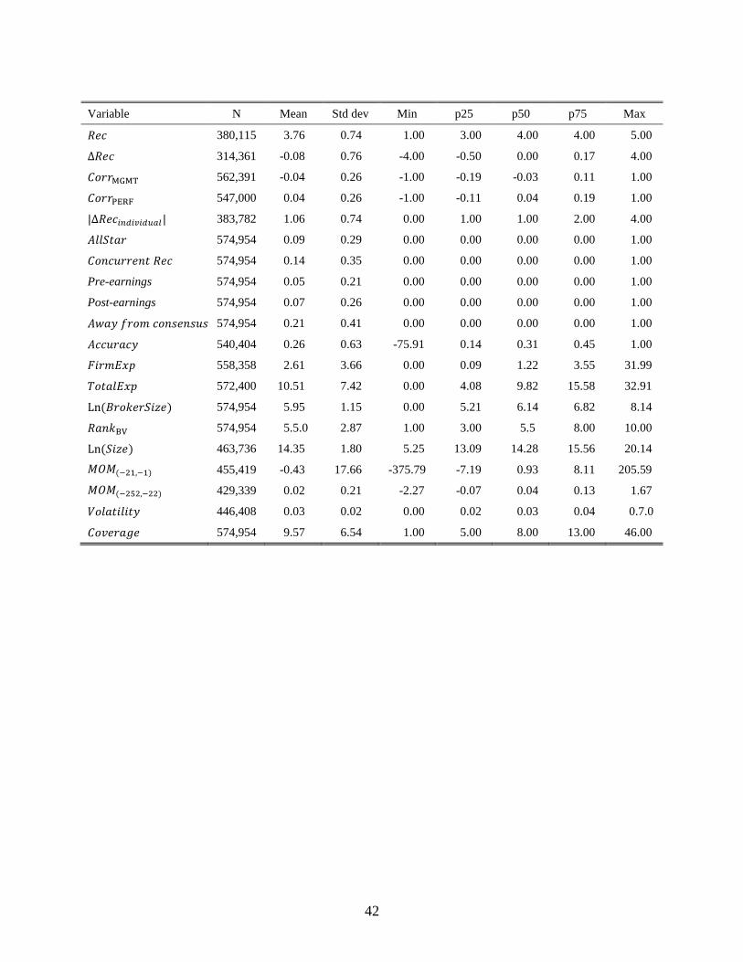
42

Variable N Mean Std dev Min p25 p50 p75 Max

𝑅𝑒𝑐 380,115 3.76 0.74 1.00 3.00 4.00 4.00 5.00

Δ𝑅𝑒c 314,361 -0.08 0.76 -4.00 -0.50 0.00 0.17 4.00

𝐶𝑜𝑟𝑟MGMT 562,391 -0.04 0.26 -1.00 -0.19 -0.03 0.11 1.00

𝐶𝑜𝑟𝑟PERF 547,000 0.04 0.26 -1.00 -0.11 0.04 0.19 1.00

|∆𝑅𝑒𝑐𝑖𝑛𝑑𝑖𝑣𝑖𝑑𝑢𝑎𝑙| 383,782 1.06 0.74 0.00 1.00 1.00 2.00 4.00

𝐴𝑙𝑙𝑆𝑡𝑎𝑟 574,954 0.09 0.29 0.00 0.00 0.00 0.00 1.00

𝐶𝑜𝑛𝑐𝑢𝑟𝑟𝑒𝑛𝑡 𝑅𝑒𝑐 574,954 0.14 0.35 0.00 0.00 0.00 0.00 1.00

Pre-earnings 574,954 0.05 0.21 0.00 0.00 0.00 0.00 1.00

Post-earnings 574,954 0.07 0.26 0.00 0.00 0.00 0.00 1.00

𝐴𝑤𝑎𝑦 𝑓𝑟𝑜𝑚 𝑐𝑜𝑛𝑠𝑒𝑛𝑠𝑢𝑠 574,954 0.21 0.41 0.00 0.00 0.00 0.00 1.00

𝐴𝑐𝑐𝑢𝑟𝑎𝑐𝑦 540,404 0.26 0.63 -75.91 0.14 0.31 0.45 1.00

𝐹𝑖𝑟𝑚𝐸𝑥p 558,358 2.61 3.66 0.00 0.09 1.22 3.55 31.99

𝑇𝑜𝑡𝑎𝑙𝐸𝑥𝑝 572,400 10.51 7.42 0.00 4.08 9.82 15.58 32.91

Ln(𝐵𝑟𝑜𝑘𝑒𝑟𝑆𝑖𝑧𝑒) 574,954 5.95 1.15 0.00 5.21 6.14 6.82 8.14

𝑅𝑎𝑛𝑘BV 574,954 5.5.0 2.87 1.00 3.00 5.5 8.00 10.00

Ln(𝑆𝑖𝑧𝑒) 463,736 14.35 1.80 5.25 13.09 14.28 15.56 20.14

𝑀𝑂𝑀(−21,−1) 455,419 -0.43 17.66 -375.79 -7.19 0.93 8.11 205.59

𝑀𝑂𝑀(−252,−22) 429,339 0.02 0.21 -2.27 -0.07 0.04 0.13 1.67

𝑉𝑜𝑙𝑎𝑡𝑖𝑙𝑖𝑡𝑦 446,408 0.03 0.02 0.00 0.02 0.03 0.04 0.7.0

𝐶𝑜𝑣𝑒𝑟𝑎𝑔𝑒 574,954 9.57 6.54 1.00 5.00 8.00 13.00 46.00

43

Table 2: Informativeness of anomaly signals

This table reports average returns and alphas on the long-short portfolios of 11 anomalies and two composite

mispricing factors. We group 11 anomalies into 2 clusters. MGMT (PERF) stands for the composite mispricing

factor of the first (second) cluster. Panel A (Panel B) reports the raw returns of Cluster 1 (Cluster 2) anomalies and

Panel C (Panel D) the Fama-French (1993) three-factor alphas of Cluster 1 (Cluster 2) anomalies. The t-statistics are

in parentheses. The sample period is 1993-2014.

Panel A: Cluster 1 (Raw returns)

MGMT NSI CEI Accrual NOA AG I/A

Long 1.25% 1.23% 1.21% 1.14% 1.19% 1.26% 1.18%

(4.16) (4.31) (4.71) (3.01) (3.49) (3.46) (3.33)

Short 0.53% 0.67% 0.76% 0.78% 0.57% 0.50% 0.59%

(1.24) (1.62) (1.83) (1.78) (1.50) (1.15) (1.41)

Long – Short 0.72% 0.57% 0.44% 0.35% 0.62% 0.76% 0.60%

(3.12) (2.63) (1.73) (2.08) (3.65) (3.89) (3.60)

Panel B: Cluster 2 (Raw returns)

PERF Distress O-score MOM GP ROA

Long 1.33% 1.29% 1.15% 1.28% 1.33% 1.33%

(3.96) (4.45) (3.15) (3.27) (3.75) (3.81)

Short 0.58% 0.81% 0.88% 0.62% 0.83% 0.51%

(1.41) (2.23) (1.97) (1.40) (2.58) (1.01)

Long – Short 0.75% 0.48% 0.27% 0.66% 0.50% 0.82%

(3.68) (2.63) (1.51) (2.10) (2.93) (3.23)

Panel C: Cluster 1 (Alphas)

MGMT NSI CEI Accrual NOA TAG I//A

Long 0.23% 0.26% 0.32% 0.00% 0.17% 0.13% 0.07%

(3.61) (3.22) (3.82) (-0.01) (1.84) (1.84) (0.86)

Short -0.62% -0.48% -0.37% -0.35% -0.55% -0.63% -0.57%

(-4.83) (-4.88) (-3.02) (-2.93) (-4.43) (-4.84) (-4.19)

Long – Short 0.86% 0.75% 0.68% 0.35% 0.72% 0.76% 0.64%

(5.75) (6.53) (5.09) (2.75) (4.28) (5.11) (4.38)

Panel D: Cluster 2 (Alphas)

PERF Distress O-score MOM GP ROA

Long 0.36% 0.37% 0.13% 0.24% 0.29% 0.32%

(3.85) (3.65) (1.33) (1.87) (3.04) (3.22)

Short -0.63% -0.33% -0.31% -0.62% -0.18% -0.77%

(-4.72) (-2.56) (-2.91) (-3.02) (-1.50) (-5.37)

Long – Short 0.99% 0.69% 0.45% 0.86% 0.47% 1.09%

(5.34) (4.03) (3.15) (2.85) (2.95) (5.64)

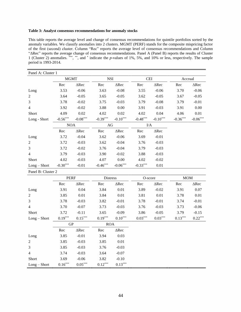
44

Table 3: Analyst consensus recommendations for anomaly stocks

This table reports the average level and change of consensus recommendations for quintile portfolios sorted by the

anomaly variables. We classify anomalies into 2 clusters. MGMT (PERF) stands for the composite mispricing factor

of the first (second) cluster. Column “Rec” reports the average level of consensus recommendations and Column

“ΔRec” reports the average change of consensus recommendations. Panel A (Panel B) reports the results of Cluster

1 (Cluster 2) anomalies. ***, **, and * indicate the p-values of 1%, 5%, and 10% or less, respectively. The sample

period is 1993-2014.

Panel A: Cluster 1

MGMT

NSI

CEI

Accrual

Rec ΔRec

Rec ΔRec

Rec ΔRec

Rec ΔRec

Long 3.53 -0.06

3.63 -0.08

3.55 -0.06

3.70 -0.06

2 3.64 -0.05

3.65 -0.05

3.62 -0.05

3.67 -0.05

3 3.78 -0.02

3.75 -0.03

3.79 -0.08

3.79 -0.01

4 3.92 -0.02

3.88 0.00

3.91 -0.03

3.91 0.00

Short 4.09 0.02

4.02 0.02

4.02 0.04

4.06 0.01

Long - Short -0.56*** -0.08***

-0.39*** -0.10***

-0.48*** -0.10***

-0.36*** -0.06***

NOA

AG

I/A

Rec ΔRec

Rec ΔRec

Rec ΔRec

Long 3.72 -0.04

3.62 -0.06

3.69 -0.01

2 3.72 -0.03

3.62 -0.04

3.76 -0.03

3 3.72 -0.02

3.76 -0.04

3.79 -0.03

4 3.79 -0.03

3.90 -0.02

3.88 -0.03

Short 4.02 -0.03

4.07 0.00

4.02 -0.02

Long – Short -0.30*** -0.01

-0.46*** -0.06***

-0.33*** 0.01

Panel B: Cluster 2

PERF

Distress

O-score

MOM

Rec ΔRec

Rec ΔRec

Rec ΔRec

Rec ΔRec

Long 3.91 0.04

3.84 0.01

3.89 -0.02

3.91 0.07

2 3.85 0.01

3.84 0.01

3.81 0.01

3.78 0.01

3 3.78 -0.03

3.82 -0.01

3.78 -0.01

3.74 -0.01

4 3.70 -0.07

3.73 -0.03

3.76 -0.03

3.73 -0.06

Short 3.72 -0.11

3.65 -0.09

3.86 -0.05

3.79 -0.15

Long – Short 0.19*** 0.15***

0.19*** 0.10***

0.03*** 0.03***

0.13*** 0.22***

GP

ROA

Rec ΔRec

Rec ΔRec

Long 3.85 -0.01

3.94 0.03

2 3.85 -0.03

3.85 0.01

3 3.85 -0.03

3.76 -0.03

4 3.74 -0.03

3.64 -0.07

Short 3.69 -0.06

3.82 -0.10

Long – Short 0.16*** 0.05***

0.12*** 0.13***

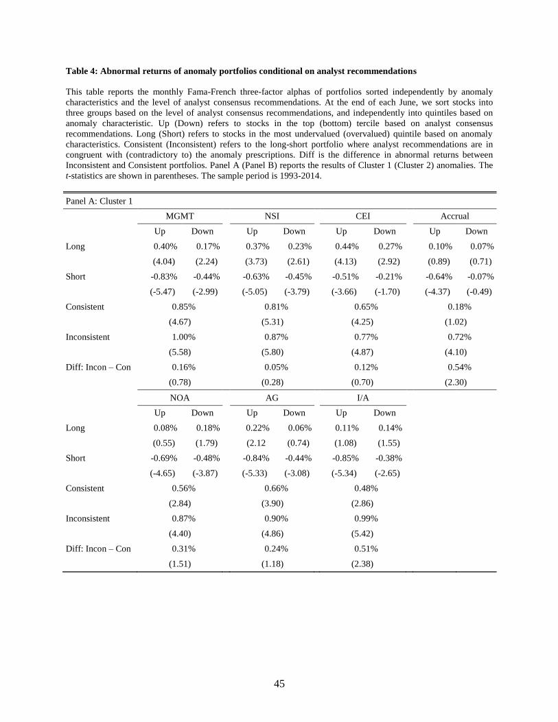
45

Table 4: Abnormal returns of anomaly portfolios conditional on analyst recommendations

This table reports the monthly Fama-French three-factor alphas of portfolios sorted independently by anomaly

characteristics and the level of analyst consensus recommendations. At the end of each June, we sort stocks into

three groups based on the level of analyst consensus recommendations, and independently into quintiles based on

anomaly characteristic. Up (Down) refers to stocks in the top (bottom) tercile based on analyst consensus

recommendations. Long (Short) refers to stocks in the most undervalued (overvalued) quintile based on anomaly

characteristics. Consistent (Inconsistent) refers to the long-short portfolio where analyst recommendations are in

congruent with (contradictory to) the anomaly prescriptions. Diff is the difference in abnormal returns between

Inconsistent and Consistent portfolios. Panel A (Panel B) reports the results of Cluster 1 (Cluster 2) anomalies. The

t-statistics are shown in parentheses. The sample period is 1993-2014.

Panel A: Cluster 1

MGMT

NSI

CEI

Accrual

Up Down

Up Down

Up Down

Up Down

Long 0.40% 0.17%

0.37% 0.23%

0.44% 0.27%

0.10% 0.07%

(4.04) (2.24)

(3.73) (2.61)

(4.13) (2.92)

(0.89) (0.71)

Short -0.83% -0.44%

-0.63% -0.45%

-0.51% -0.21%

-0.64% -0.07%

(-5.47) (-2.99)

(-5.05) (-3.79)

(-3.66) (-1.70)

(-4.37) (-0.49)

Consistent 0.85%

0.81%

0.65%

0.18%

(4.67)

(5.31)

(4.25)

(1.02)

Inconsistent 1.00%

0.87%

0.77%

0.72%

(5.58)

(5.80)

(4.87)

(4.10)

Diff: Incon – Con 0.16%

0.05%

0.12%

0.54%

(0.78)

(0.28)

(0.70)

(2.30)

NOA

AG

I/A

Up Down

Up Down

Up Down

Long 0.08% 0.18%

0.22% 0.06%

0.11% 0.14%

(0.55) (1.79)

(2.12 (0.74)

(1.08) (1.55)

Short -0.69% -0.48%

-0.84% -0.44%

-0.85% -0.38%

(-4.65) (-3.87)

(-5.33) (-3.08)

(-5.34) (-2.65)

Consistent 0.56%

0.66%

0.48%

(2.84)

(3.90)

(2.86)

Inconsistent 0.87%

0.90%

0.99%

(4.40)

(4.86)

(5.42)

Diff: Incon – Con 0.31%

0.24%

0.51%

(1.51)

(1.18)

(2.38)

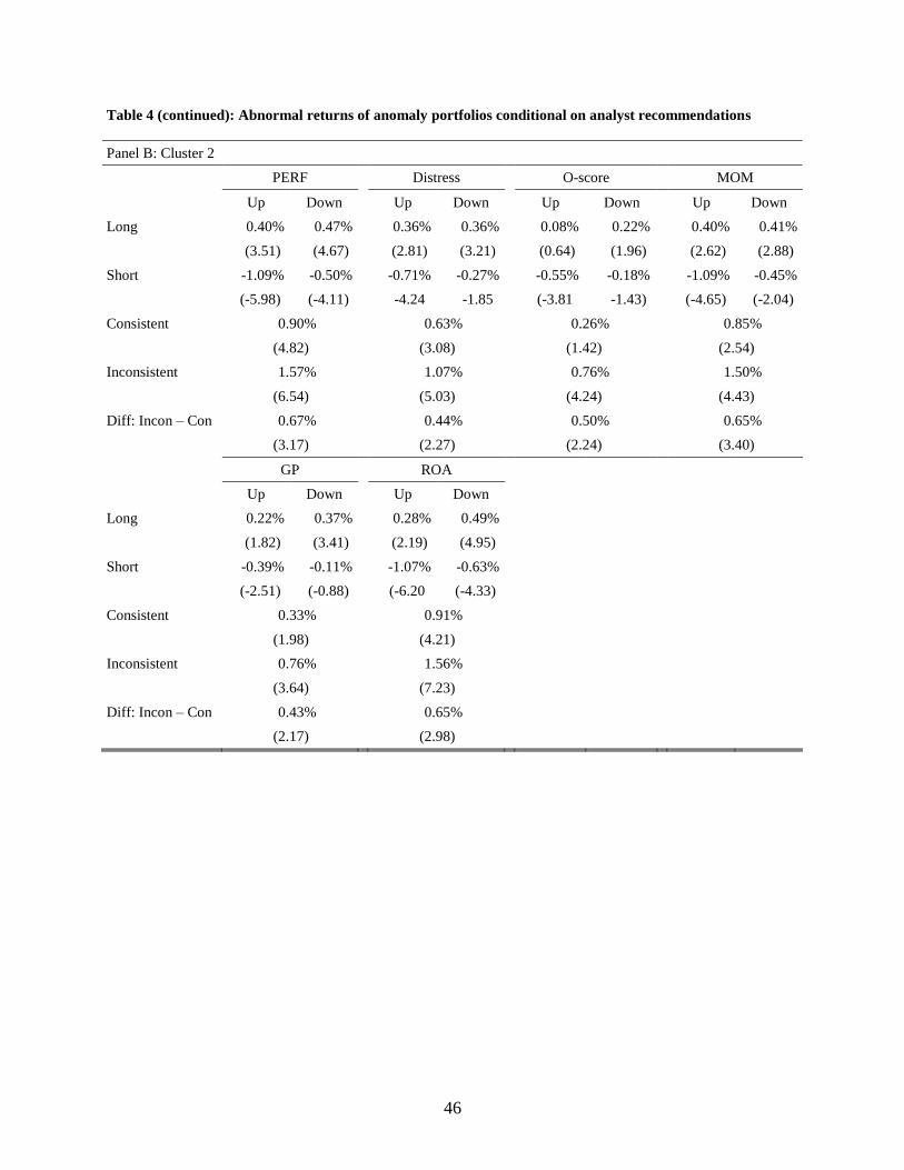
46

Table 4 (continued): Abnormal returns of anomaly portfolios conditional on analyst recommendations

Panel B: Cluster 2

PERF

Distress

O-score

MOM

Up Down

Up Down

Up Down

Up Down

Long 0.40% 0.47%

0.36% 0.36%

0.08% 0.22%

0.40% 0.41%

(3.51) (4.67)

(2.81) (3.21)

(0.64) (1.96)

(2.62) (2.88)

Short -1.09% -0.50%

-0.71% -0.27%

-0.55% -0.18%

-1.09% -0.45%

(-5.98) (-4.11)

-4.24 -1.85

(-3.81 -1.43)

(-4.65) (-2.04)

Consistent 0.90%

0.63%

0.26%

0.85%

(4.82)

(3.08)

(1.42)

(2.54)

Inconsistent 1.57%

1.07%

0.76%

1.50%

(6.54)

(5.03)

(4.24)

(4.43)

Diff: Incon – Con 0.67%

0.44%

0.50%

0.65%

(3.17)

(2.27)

(2.24)

(3.40)

GP

ROA

Up Down

Up Down

Long 0.22% 0.37%

0.28% 0.49%

(1.82) (3.41)

(2.19) (4.95)

Short -0.39% -0.11%

-1.07% -0.63%

(-2.51) (-0.88)

(-6.20 (-4.33)

Consistent 0.33%

0.91%

(1.98)

(4.21)

Inconsistent 0.76%

1.56%

(3.64)

(7.23)

Diff: Incon – Con 0.43%

0.65%

(2.17)

(2.98)

47

Table 5: Fama-MacBeth Regressions

This table reports the Fama and MacBeth (1973) regressions of stock returns on the anomaly characteristics

interacted with analyst consensus recommendations. Long (short) is a dummy variable that equals one for stocks in

the top (bottom) quintile based on the anomaly signal. RecUp (RecDown) is a dummy that equals one for stocks in

the top (bottom) tercile based on the consensus recommendation. We run the Fama-MacBeth regression as follows:

𝑅𝑒𝑡𝑖,𝑡+1 = 𝛼 + 𝛽1𝐿𝑜𝑛𝑔 × 𝑅𝑒𝑐𝑈𝑝 + 𝛽2𝐿𝑜𝑛𝑔 × 𝑅𝑒𝑐𝑀𝑖𝑑 + 𝛽3𝐿𝑜𝑛𝑔 × 𝑅𝑒𝑐𝐷𝑜𝑤𝑛 + 𝛽4𝑆ℎ𝑜𝑟𝑡 × 𝑅𝑒𝑐𝑈𝑝

+ 𝛽5𝑆ℎ𝑜𝑟𝑡 × 𝑅𝑒𝑐𝑀𝑖𝑑 + 𝛽6𝑆ℎ𝑜𝑟𝑡 × 𝑅𝑒𝑐𝐷𝑜𝑤𝑛 + ∑ 𝛽𝑘𝑋𝑘,𝑖,𝑡 + 𝜖𝑖,𝑡+1,

where 𝑋𝑘,𝑖,𝑡 stands for a set of firm controls, including firm size, short-term reversal, book-to-market ratio,

idiosyncratic volatility, past 12-month turnover, analyst forecast dispersion, and last month maximum return. Panel

A (Panel B) reports the results of Cluster 1 (Cluster 2) anomalies. The significance of the estimates is based on

Newey-West (1987) adjusted t-statistics. *, **, and *** indicate the significance levels at the 10%, 5%, and 1% levels,

respectively. The sample period is from January 1993 to December 2014.

Dependent Variable: Excess Return (%)

Panel A: Cluster 1

MGMT NSI CEI Accrual NOA AG I/A

𝐿𝑜𝑛𝑔 × 𝑅𝑒𝑐𝑈𝑝 0.272** 0.083 0.124 0.421*** -0.144 0.241* 0.128

(2.16) (0.70) (0.92) (2.92) (-0.81) (1.66) (1.04)

𝐿𝑜𝑛𝑔 × 𝑅𝑒𝑐𝑀𝑖𝑑 0.340* 0.007 0.176 0.279 0.109 0.438* 0.161

(1.68) (0.06) (1.27) (1.26) (0.64) (1.95) (0.67)

𝐿𝑜𝑛𝑔 × 𝑅𝑒𝑐𝐷𝑜𝑤𝑛 0.295** 0.016 -0.033 0.558* 0.040 0.354** 0.583***

(2.49) (0.11) (-0.20) (1.90) (0.23) (2.12) (2.87)

𝑆ℎ𝑜𝑟𝑡 × 𝑅𝑒𝑐𝑈𝑝 -0.688*** -0.536*** -0.470*** -0.304* -0.550*** -0.760*** -0.477**

(-4.37) (-4.89) (-3.60) (-1.87) (-3.43) (-3.93) (-2.36)

𝑆ℎ𝑜𝑟𝑡 × 𝑅𝑒𝑐𝑀𝑖𝑑 0.166 0.125 0.036 0.223 -0.224 -0.161 0.275

(0.69) (0.51) (0.23) (0.78) (-1.60) (-1.03) (1.01)

𝑆ℎ𝑜𝑟𝑡 × 𝑅𝑒𝑐𝐷𝑜𝑤𝑛 -0.403** -0.571*** -0.195 -0.045 -0.409** -0.522** -0.389*

(-2.16) (-3.31) (-0.91) (-0.20) (-2.54) (-2.29) (-1.93)

𝑆ℎ𝑜𝑟𝑡-𝑡𝑒𝑟𝑚 𝑟𝑒𝑣𝑒𝑟𝑠𝑎𝑙 -1.484** -1.538** -1.464** -1.514** -1.511** -1.567** -1.639***

(-2.33) (-2.48) (-2.34) (-2.43) (-2.42) (-2.50) (-2.68)

𝐿𝑛(𝑆𝑖𝑧𝑒) -0.070 -0.077 -0.073 -0.063 -0.073 -0.069 -0.055

(-1.32) (-1.54) (-1.49) (-1.18) (-1.38) (-1.33) (-1.06)

𝐿𝑛(𝐵/𝑀) -0.050 -0.053 -0.046 -0.036 -0.041 -0.055 -0.040

(-0.39) (-0.41) (-0.35) (-0.28) (-0.33) (-0.43) (-0.30)

𝐼𝑉𝑂𝐿 -9.001 -12.878 -11.743 -12.212 -10.896 -10.719 -9.256

(-0.94) (-1.45) (-1.30) (-1.29) (-1.15) (-1.17) (-0.99)

𝑇𝑢𝑟𝑛𝑜𝑣𝑒𝑟 0.490 0.339 0.404 0.154 0.374 0.370 0.093

(0.45) (0.31) (0.37) (0.14) (0.34) (0.35) (0.09)

𝐷𝑖𝑠𝑝𝑒𝑟𝑠𝑖𝑜𝑛 0.000 0.062 0.111 -0.149 0.243 0.214 0.044

(0.00) (0.15) (0.25) (-0.39) (0.60) (0.57) (0.11)

𝑀𝑎𝑥𝑅𝑒𝑡𝑢𝑟𝑛 -0.764 0.069 -0.641 -1.000 -0.332 -0.092 -1.102

(-0.29) (0.03) (-0.24) (-0.36) (-0.12) (-0.04) (-0.43)

N 520,034 520,034 520,034 520,034 520,034 520,034 520,034

Adjusted R2 0.072 0.072 0.071 0.074 0.074 0.074 0.075

48

Table 5 (continued): Fama-MacBeth Regressions

Dependent variable: Excess returns (%)

Panel B: Cluster 2

PERF Distress O-score MOM GP ROA

𝐿𝑜𝑛𝑔 × 𝑅𝑒𝑐𝑈𝑝 0.281** 0.203 0.186 0.275 0.213 0.352**

(2.42) (1.20) (1.46) (1.37) (1.50) (2.54)

𝐿𝑜𝑛𝑔 × 𝑅𝑒𝑐𝑀𝑖𝑑 0.398*** 0.102 0.232 0.664*** 0.606** 0.489***

(3.13) (0.77) (1.36) (3.24) (2.18) (3.62)

𝐿𝑜𝑛𝑔 × 𝑅𝑒𝑐𝐷𝑜𝑤𝑛 0.323* 0.189 0.191 0.510** 0.511*** 0.354**

(1.96) (1.36) (1.40) (2.01) (3.65) (2.24)

𝑆ℎ𝑜𝑟𝑡 × 𝑅𝑒𝑐𝑈𝑝 -0.756*** -0.779** -0.073 -0.591*** -0.400* -0.921***

(-3.19) (-2.58) (-0.36) (-2.67) (-1.83) (-3.17)

𝑆ℎ𝑜𝑟𝑡 × 𝑅𝑒𝑐𝑀𝑖𝑑 0.053 0.238 0.108 0.002 -0.080 -0.087

(0.23) (1.02) (0.41) (0.01) (-0.42) (-0.22)

𝑆ℎ𝑜𝑟𝑡 × 𝑅𝑒𝑐𝐷𝑜𝑤𝑛 -0.437*** -0.339** 0.211 -0.169 -0.346 -0.088

(-2.80) (-2.15) (1.26) (-0.86) (-1.43) (-0.33)

𝑆ℎ𝑜𝑟𝑡-𝑡𝑒𝑟𝑚 𝑟𝑒𝑣𝑒𝑟𝑠𝑎𝑙 -1.625*** -1.506** -1.511** -1.359** -1.547** -1.701***

(-2.61) (-2.43) (-2.41) (-2.15) (-2.52) (-2.68)

𝐿𝑛(𝑆𝑖𝑧𝑒) -0.069 -0.066 -0.066 -0.060 -0.063 -0.080

(-1.36) (-1.26) (-1.27) (-1.12) (-1.18) (-1.64)

𝐿𝑛(𝐵/𝑀) 0.035 -0.010 -0.018 0.048 0.021 0.007

(0.27) (-0.08) (-0.14) (0.42) (0.16) (0.05)

𝐼𝑉𝑂𝐿 -12.760 -14.032 -14.855 -13.182 -13.927 -11.836

(-1.38) (-1.54) (-1.58) (-1.50) (-1.54) (-1.21)

𝑇𝑢𝑟𝑛𝑜𝑣𝑒𝑟 -0.053 0.004 0.075 -0.048 -0.121 0.140

(-0.05) (0.00) (0.07) (-0.05) (-0.11) (0.13)

𝐷𝑖𝑠𝑝𝑒𝑟𝑠𝑖𝑜𝑛 0.277 0.414 0.168 0.302 0.314 0.385

(0.70) (0.97) (0.40) (0.78) (0.81) (0.96)

𝑀𝑎𝑥𝑅𝑒𝑡𝑢𝑟𝑛 0.363 0.010 0.162 -0.172 -0.198 0.369

(0.14) (0.00) (0.06) (-0.07) (-0.08) (0.14)

N 520,034 520,034 520,034 520,034 520,034 520,034

Adjusted R2 0.075 0.070 0.073 0.078 0.077 0.078

49

Table 6: Earnings announcement returns

This table reports the two-day cumulative abnormal return (CAR [0, +1]) around quarterly earnings announcements

of portfolios sorted independently by anomaly characteristics and the level of analyst consensus recommendations.

At the end of each June, we sort stocks into three groups based on the level of analyst consensus recommendations,

and independently into quintiles based on anomaly characteristics. Up (Down) refers to stocks in the top (bottom)

tercile based on analyst consensus recommendations. Long (Short) refers to stocks in the most undervalued

(overvalued) quintile based on anomaly characteristics. Consistent (Inconsistent) refers to the long-short portfolio

where analyst recommendations are in congruent with (contradictory to) the anomaly prescriptions. Diff is the

difference in CAR [0, +1] between the Inconsistent and Consistent portfolios. Panel A (Panel B) reports the results

of Cluster 1 (Cluster 2) anomalies. The t-statistics are shown in parentheses. The sample period is 1993-2014.

Panel A: Cluster 1

MGMT

NSI

CEI

Accrual

Up Down

Up Down

Up Down

Up Down

Long 0.11% 0.10%

0.18% 0.15%

0.29% 0.19%

-0.16% 0.12%

(1.06) (1.05)

(1.64) (2.03)

(3.40) (2.73)

(-1.33) (1.17)

Short 0.12% 0.00%

-0.09% 0.00%

0.17% 0.20%

0.14% 0.22%

(1.30) (0.03)

(-0.98) (-0.03)

(2.13) (1.69)

(1.37) (1.50)

Consistent 0.11%

0.19%

0.09%

-0.38%

(0.48)

(0.87)

(0.57)

(-1.88)

Inconsistent -0.03%

0.24%

0.02%

-0.02%

-(0.19)

(1.65)

(0.12)

(-0.12)

Diff: Incon – Con -0.14%

0.06%

-0.08%

0.36%

(-0.61)

(0.26)

(-0.43)

(1.78)

NOA

AG

I/A

Up Down

Up Down

Up Down

Long -0.10% 0.09%

-0.24% 0.10%

-0.07% 0.22%

(-1.13) (0.95)

(-2.65 1.11

(-0.61) 2.24

Short 0.12% -0.06%

0.04% -0.05%

-0.03% -0.07%

(0.98) (-0.62)

(0.37) -0.29

(-0.27) -0.73

Consistent -0.04%

-0.20%

0.00%

(-0.26)

(-1.13)

(-0.03)

Inconsistent -0.03%

0.06%

0.25%

(-0.15)

(0.38)

(1.70)

Diff: Incon – Con 0.01%

0.25%

0.25%

(0.09)

(1.49)

(1.21)

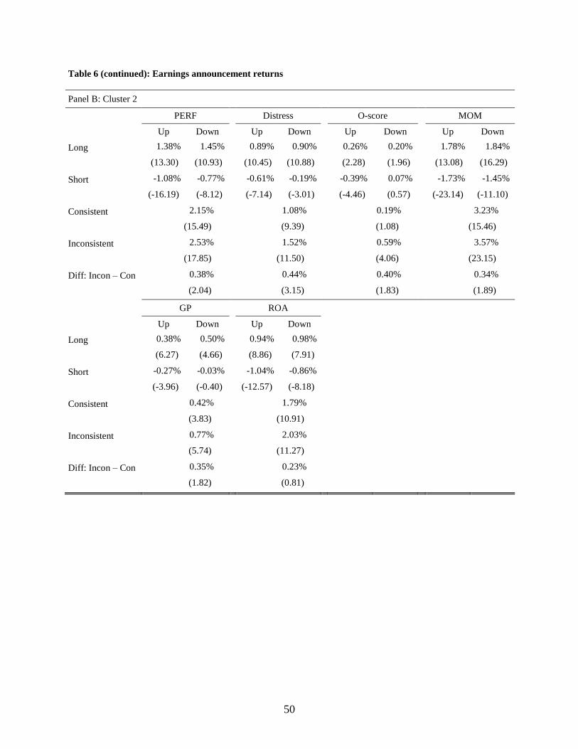
50

Table 6 (continued): Earnings announcement returns

Panel B: Cluster 2

PERF

Distress

O-score

MOM

Up Down

Up Down

Up Down

Up Down

Long 1.38% 1.45% 0.89% 0.90% 0.26% 0.20% 1.78% 1.84%

(13.30) (10.93) (10.45) (10.88) (2.28) (1.96) (13.08) (16.29)

Short -1.08% -0.77% -0.61% -0.19% -0.39% 0.07% -1.73% -1.45%

(-16.19) (-8.12) (-7.14) (-3.01) (-4.46) (0.57) (-23.14) (-11.10)

Consistent 2.15% 1.08% 0.19% 3.23%

(15.49) (9.39) (1.08) (15.46)

Inconsistent 2.53% 1.52% 0.59% 3.57%

(17.85) (11.50) (4.06) (23.15)

Diff: Incon – Con 0.38% 0.44% 0.40% 0.34%

(2.04) (3.15) (1.83) (1.89)

GP

ROA

Up Down

Up Down

Long 0.38% 0.50% 0.94% 0.98%

(6.27) (4.66) (8.86) (7.91)

Short -0.27% -0.03% -1.04% -0.86%

(-3.96) (-0.40) (-12.57) (-8.18)

Consistent 0.42% 1.79%

(3.83) (10.91)

Inconsistent 0.77% 2.03%

(5.74) (11.27)

Diff: Incon – Con 0.35% 0.23%

(1.82) (0.81)

51

Table 7: Determinants of analyst skills

This table presents panel regression results of analyst skills on analyst and firm characteristics, where skill is

measured as the correlation between individual analyst’ recommendations and two mispricing scores among stocks

covered by the analyst. We conduct the panel regression as follows:

𝐶𝑜𝑟𝑟𝑠 = 𝛼 + 𝛽1𝐴𝑙𝑙𝑆𝑡𝑎𝑟 + 𝛽2𝐴𝑤𝑎𝑦 𝑓𝑟𝑜𝑚 𝑐𝑜𝑛𝑠𝑒𝑛𝑠𝑢𝑠 + 𝛽3𝐴𝑐𝑐𝑢𝑟𝑎𝑐𝑦 + 𝛽4𝐹𝑖𝑟𝑚𝐸𝑥𝑝

+𝛽5𝑇𝑜𝑡𝑎𝑙𝐸𝑥𝑝 + 𝛽6𝐿𝑛(𝐵𝑟𝑜𝑘𝑒𝑟𝑆𝑖𝑧𝑒) + 𝛽7𝐴𝑣𝑒𝑟𝑎𝑔𝑒 𝑆𝑖𝑧𝑒 + 𝛽8𝐶𝑜𝑣𝑒𝑟𝑎𝑔𝑒 + 𝜖𝑖,𝑡+1,

where 𝐶𝑜𝑟𝑟𝑠 stands for the correlation between individual analyst’ recommendations and two mispricing scores,

MGMT or PERF, among all stocks covered by the analyst. All other variables are defined in Table 1. Standard

errors are clustered by analyst, and t-statistics are reported in parentheses. *, **, and *** indicate the significance

levels at the 10%, 5%, and 1% levels, respectively. The sample period is from 1993 to 2014.

𝐶𝑜𝑟𝑟𝑀𝐺𝑀𝑇

𝐶𝑜𝑟𝑟𝑃𝐸𝑅𝐹

𝐴𝑙𝑙𝑆𝑡𝑎𝑟 -0.004 -0.014** -0.003 -0.011*

0.007 0.012** 0.006 0.012*

(-0.74) (-2.21) (-0.56) (-1.75)

(1.43) (2.00) (1.21) (1.85)

𝐴𝑤𝑎𝑦 𝑓𝑟𝑜𝑚 𝑐𝑜𝑛𝑠𝑒𝑛𝑠𝑢𝑠 -0.001 -0.000 -0.001 -0.001

-0.001 -0.004 -0.001 -0.003

(-0.25) (-0.03) (-0.41) (-0.30)

(-0.39) (-1.14) (-0.17) (-1.00)

𝐴𝑐𝑐𝑢𝑟𝑎𝑐𝑦 0.004** 0.002 0.005** 0.002

0.006*** 0.005** 0.005*** 0.005**

(2.10) (0.63) (2.21) (0.75)

(3.01) (2.42) (2.78) (2.14)

𝐹𝑖𝑟𝑚𝐸𝑥p -0.000 -0.001 -0.000 -0.001

-0.001* -0.001** -0.001* -0.001*

(-1.06) (-1.49) (-0.97) (-1.47)

(-1.95) (-2.17) (-1.66) (-1.68)

𝑇𝑜𝑡𝑎𝑙𝐸𝑥𝑝 -0.000* -0.000 -0.000** -0.001**

0.001*** -0.000 0.001*** 0.001**

(-1.78) (-0.55) (-2.20) (-1.99)

(2.73) (-0.02) (3.65) (2.55)

𝐿𝑛(𝐵𝑟𝑜𝑘𝑒𝑟𝑆𝑖𝑧𝑒) -0.008*** -0.007*** -0.008*** -0.007***

0.004*** 0.002 0.004*** 0.002

(-5.45) (-3.81) (-5.26) (-3.69)

(3.13) (1.18) (2.74) (1.21)

𝐶𝑜𝑣𝑒𝑟𝑎𝑔𝑒 -0.000 -0.000** -0.000 -0.000**

0.000 0.000* 0.000 0.000

(-0.75) (-2.30) (-0.63) (-2.37)

(1.56) (1.66) (0.94) (1.45)

𝐴𝑣𝑒𝑟𝑎𝑔𝑒 𝑆𝑖𝑧𝑒 0.000** 0.000* 0.000** 0.000

0.000 -0.000 0.000 0.000

(2.45) (1.74) (2.13) (1.29)

(0.16) (-0.46) (0.77) (0.05)

Intercept 0.018** 0.013 0.017* -0.021

0.003 0.022* 0.004 0.049***

(2.05) (1.17) (1.88) (-1.43)

(0.33) (1.93) (0.41) (3.45)

Year FE No Yes No Yes

No Yes No Yes

Analyst FE No No Yes Yes

No No Yes Yes

N 34,866 34,866 34,866 34,866

33,705 33,705 33,705 33,705

Adjusted R2 0.0020 0.0016 0.0018 0.0042

0.0010 0.0005 0.0009 0.0055

52

Table 8: Market reactions to skilled analysts’ recommendation announcements

This table presents the panel regression of analyst recommendation announcement returns on our measure of analyst

skill, where skill is measured as the correlation between individual analyst’ recommendations and two mispricing

scores among stocks covered by the analyst. We estimate the panel regression as follows:

𝑌𝑖 = 𝛼 + 𝛽1𝐶𝑜𝑟𝑟𝑠 + 𝛽2|∆𝑅𝑒𝑐𝑖𝑛𝑑𝑖𝑣𝑖𝑑𝑢𝑎𝑙| + 𝛽3𝐴𝑙𝑙𝑆𝑡𝑎𝑟 + 𝛽4𝐶𝑜𝑛𝑐𝑢𝑟𝑟𝑒𝑛𝑡 𝑅𝑒𝑐

+𝛽5𝑃𝑟𝑒-𝑒𝑎𝑟𝑛𝑖𝑛𝑔𝑠 + 𝛽6𝑃𝑜𝑠𝑡-𝑎𝑟𝑛𝑖𝑛𝑔𝑠 + 𝛽7𝐴𝑤𝑎𝑦 𝑓𝑟𝑜𝑚 𝑐𝑜𝑛𝑠𝑒𝑛𝑠𝑢𝑠 + 𝛽8𝐴𝑐𝑐𝑢𝑟𝑎𝑐𝑦

+𝛽9𝐹𝑖𝑟𝑚𝐸𝑥𝑝 + 𝛽10𝑇𝑜𝑡𝑎𝑙𝐸𝑥𝑝 + ∑ 𝛽𝑘𝑋𝑘,𝑖,𝑡 + 𝜖𝑖,𝑡+1,

where 𝑌𝑖 is the 2-day cumulative abnormal return (𝐶𝐴𝑅[0, +1]) or the 2-day absolute cumulative abnormal return (|𝐶𝐴𝑅[0, +1]|) around recommendation announcements. 𝐶𝑜𝑟𝑟𝑠 is the correlation between individual

analyst’ recommendations and two composite mispricing scores, MGMT or PERF, among stocks covered by the analyst. All other variables are defined in Table 1. 𝑋𝑘,𝑖,𝑡 stands for the vector of firm characteristics, including

𝐿𝑛(𝑆𝑖𝑧𝑒) , 𝑅𝑎𝑛𝑘𝐵𝑉 , volatility, 𝑀𝑂𝑀(−21,−1) , and 𝑀𝑂𝑀(−252,−22). Panel A reports the results for upgrade

recommendation changes, and Panel B for downgrade recommendation changes. Panel C pools together upgrade

and downgrade recommendation changes, and uses the absolute value of cumulative abnormal return (|𝐶𝐴𝑅[0, +1]|)

as the dependent variable. Standard errors are clustered at the analyst level, and t-statistics are reported in

parentheses. *, **, and *** indicate the significance levels at the 10%, 5%, and 1% levels, respectively. The sample

period is 1993-2014.

53

Table 8 (continued): Market reactions to skilled analysts’ recommendation announcements

Panel A: Upgrade recommendation changes (𝐶𝐴𝑅[0, +1])

Cluster 1

Cluster 2

𝐶𝑜𝑟𝑟𝑀𝐺𝑀𝑇 -0.000 0.001 -0.001

(-0.43) (0.42) (-0.58)

𝐶𝑜𝑟𝑟𝑃𝐸𝑅𝐹

0.002** 0.003** 0.004**

(2.24) (1.97) (2.07)

|∆𝑅𝑒𝑐𝑖𝑛𝑑𝑖𝑣𝑖𝑑𝑢𝑎𝑙| 0.004*** 0.005*** 0.005***

0.004*** 0.005*** 0.005***

(8.14) (8.66) (6.51)

(8.26) (8.80) (6.65)

𝐴𝑙𝑙𝑆𝑡𝑎𝑟 0.006*** 0.003*** 0.002*

0.006*** 0.003*** 0.003**

(8.73) (2.88) (1.65)

(8.75) (3.04) (2.17)

𝐶𝑜𝑛𝑐𝑢𝑟𝑟𝑒𝑛𝑡 𝑅𝑒𝑐 0.014*** 0.013*** 0.014***

0.014*** 0.014*** 0.014***

(28.77) (26.26) (18.49)

(28.61) (26.06) (17.89)

𝑃𝑟𝑒-𝑒𝑎𝑟𝑛𝑖𝑛𝑔𝑠 0.004*** 0.004*** 0.005***

0.004*** 0.003*** 0.005***

(4.12) (3.38) (2.94)

(3.77) (2.97) (2.87)

𝑃𝑜𝑠𝑡-𝑒𝑎𝑟𝑛𝑖𝑛𝑔𝑠 0.002*** 0.003*** 0.003***

0.003*** 0.004*** 0.004***

(2.85) (4.06) (2.63)

(3.05) (4.32) (2.79)

𝐴𝑤𝑎𝑦 𝑓𝑟𝑜𝑚 𝑐𝑜𝑛𝑠𝑒𝑛𝑠𝑢𝑠 0.002*** 0.001*** 0.002**

0.001*** 0.001* 0.002**

(3.51) (2.65) (2.32)

(3.11) (1.96) (2.18)

𝐴𝑐𝑐𝑢𝑟𝑎𝑐𝑦 0.001 -0.000 0.001

0.001 -0.000 0.000

(1.52) (-0.29) (0.65)

(1.46) (-0.45) (0.09)

𝐹𝑖𝑟𝑚𝐸𝑥𝑝 0.000** -0.000 0.000

0.000* -0.000 0.000

(2.08) (-0.30) (0.17)

(1.86) (-0.75) (0.19)

𝑇𝑜𝑡𝑎𝑙𝐸𝑥𝑝 0.000*** 0.004*** 0.003

0.000*** 0.004*** 0.003

(3.26) (4.24) (1.45)

(3.72) (4.23) (1.34)

𝐿𝑛(𝐵𝑟𝑜𝑘𝑒𝑟𝑆𝑖𝑧𝑒) 0.003*** 0.001*** 0.002***

0.003*** 0.001*** 0.002**

(15.36) (3.47) (2.72)

(15.02) (3.18) (2.37)

𝐶𝑜𝑣𝑒𝑟𝑎𝑔𝑒 -0.001*** -0.001*** -0.001***

-0.001*** -0.001*** -0.001***

(-7.57) (-12.57) (-5.17)

(-7.44) (-12.40) (-5.16)

Intercept -0.036*** -0.025*** (0.02)

-0.035*** -0.024*** (0.02)

(-7.75) (-4.78) (-1.49)

(-7.88) (-4.53) (-1.20)

Firm controls Yes Yes Yes

Yes Yes Yes

Year FE Yes Yes Yes

Yes Yes Yes

Firm FE Yes No Yes

Yes No Yes

Analyst FE No Yes Yes

No Yes Yes

N 84,322 84,322 84,322

81,942 81,942 81,942

Adjusted R2 0.046 0.051 0.041 0.044 0.049 0.038

54

Table 8 (continued): Market reactions to skilled analysts’ recommendation announcements

Panel B: Downgrade recommendation changes (𝐶𝐴𝑅[0, +1])

Cluster 1

Cluster 2

𝐶𝑜𝑟𝑟𝑀𝐺𝑀𝑇 -0.000 -0.001 -0.001

(-0.27) (-0.38) (-0.52)

𝐶𝑜𝑟𝑟𝑃𝐸𝑅𝐹

-0.005*** -0.006*** -0.007***

(-3.57) (-2.92) (-2.71)

|∆𝑅𝑒𝑐𝑖𝑛𝑑𝑖𝑣𝑖𝑑𝑢𝑎𝑙| -0.008*** -0.013*** -0.013***

-0.008*** -0.013*** -0.013***

(-12.31) (-13.96) (-10.11)

(-12.44) (-13.78) (-10.21)

𝐴𝑙𝑙𝑆𝑡𝑎𝑟 -0.008*** -0.003** -0.002

-0.007*** -0.003* -0.001

(-7.47) (-2.02) (-0.73)

(-7.14) (-1.70) (-0.56)

𝐶𝑜𝑛𝑐𝑢𝑟𝑟𝑒𝑛𝑡 𝑅𝑒𝑐 -0.038*** -0.038*** -0.035***

-0.039*** -0.038*** -0.035***

(-46.54) (-43.21) (-28.85)

(-46.69) (-43.30) (-29.02)

𝑃𝑟𝑒-𝑒𝑎𝑟𝑛𝑖𝑛𝑔𝑠 -0.002 0.001 0.001

-0.002 -0.000 0.001

(-1.14) (0.41) (0.69)

(-1.50) (-0.15) (0.48)

𝑃𝑜𝑠𝑡-𝑒𝑎𝑟𝑛𝑖𝑛𝑔𝑠 -0.011*** -0.009*** -0.009***

-0.011*** -0.010*** -0.009***

(-9.93) (-7.72) (-5.55)

(-9.90) (-7.90) (-5.20)

𝐴𝑤𝑎𝑦 𝑓𝑟𝑜𝑚 𝑐𝑜𝑛𝑠𝑒𝑛𝑠𝑢𝑠 0.002*** 0.001* 0.002*

0.002*** 0.002** 0.002

(3.24) (1.85) (1.87)

(3.34) (2.15) (1.64)

𝐴𝑐𝑐𝑢𝑟𝑎𝑐𝑦 -0.001 -0.001 0.000

-0.001** -0.001 -0.001

(-1.61) (-0.83) (0.25)

(-1.99) (-0.93) (-0.86)

𝐹𝑖𝑟𝑚𝐸𝑥𝑝 -0.000*** -0.000 -0.009***

-0.000*** -0.000 -0.011**

(-2.94) (-0.48) (-2.95)

(-2.85) (-0.51) (-2.55)

𝑇𝑜𝑡𝑎𝑙𝐸𝑥𝑝 -0.000*** 0.009*** 0.017***

-0.000*** 0.008*** 0.018***

(-3.12) (-7.64) (4.76)

(-2.88) (6.99) (3.96)

𝐿𝑛(𝐵𝑟𝑜𝑘𝑒𝑟𝑆𝑖𝑧𝑒) -0.005*** -0.002*** -0.000

-0.005*** -0.002*** -0.000

(-15.72) (-3.20) (-0.27)

(-15.52) (-3.03) (-0.01)

𝐶𝑜𝑣𝑒𝑟𝑎𝑔𝑒 -0.001*** -0.000*** -0.001***

-0.001*** -0.000*** -0.001***

(-12.87) (-2.62) (-6.90)

(-12.40) (-2.74) (-6.65)

Intercept 0.113*** 0.103*** 0.023

0.117*** 0.104*** 0.014

(12.41) (9.78) (0.87)

(12.48) (9.63) (0.40)

Firm controls Yes Yes Yes

Yes Yes Yes

Year FE Yes Yes Yes

Yes Yes Yes

Firm FE Yes No Yes

Yes No Yes

Analyst FE No Yes Yes

No Yes Yes

N 99,191 99,191 99,191

96,571 96,571 96,571

Adjust R2 0.168 0.212 0.165 0.168 0.210 0.162

55

Table 9: Subsample tests in post-publication periods

Panel A reports Fama-French three-factors adjusted returns for quintile portfolios sorted by 11 anomalies. Panel B

reports the average level and change of analyst consensus recommendations across quintile portfolios. Column “Rec”

reports the average level of consensus recommendations and Column “ΔRec” reports the average change of

consensus recommendations. We use the post publication periods for the test. ***, **, and * indicate the p-values of

1%, 5%, and 10% or less, respectively.

Panel A: Alpha

NSI CEI Accrual NOA AG I/A

Long 0.26% 0.10% 0.03% -0.08% 0.16% -0.01%

(3.20) (1.00) (0.29) (-0.56) (1.66) (-0.11)

Short -0.49% -0.27% -0.33% -0.22% -0.20% -0.30%

(-4.89) (-2.12) (-2.49) (-1.79) (-1.31) (-1.89)

Long – Short 0.75% 0.37% 0.36% 0.14% 0.36% 0.29%

(6.53) (2.28) (2.56) (0.67) (1.97) (1.64)

Distress O-score MOM GP ROA

Long 0.09% -0.03% 0.24% 0.16% -0.02%

(0.93) (-0.29) (1.86) (1.02) (-0.28)

Short 0.20% 0.16% -0.62% 0.60% -0.38%

(1.36) (1.07) (-3.02) (3.30) (-2.17)

Long – Short -0.11% -0.20% 0.86% -0.44% 0.35%

(-0.57) (-0.94) (2.85) (-1.78) (1.91)

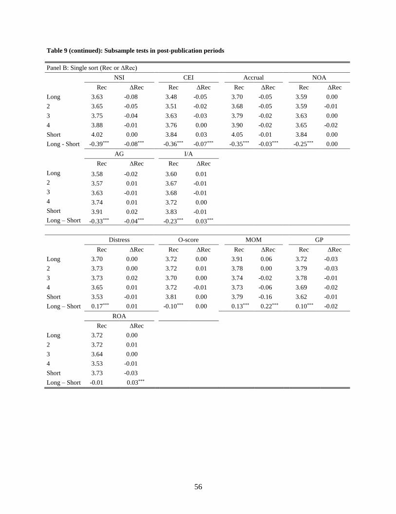
56

Table 9 (continued): Subsample tests in post-publication periods

Panel B: Single sort (Rec or ΔRec)

NSI

CEI

Accrual

NOA

Rec ΔRec

Rec ΔRec

Rec ΔRec

Rec ΔRec

Long 3.63 -0.08

3.48 -0.05

3.70 -0.05

3.59 0.00

2 3.65 -0.05

3.51 -0.02

3.68 -0.05

3.59 -0.01

3 3.75 -0.04

3.63 -0.03

3.79 -0.02

3.63 0.00

4 3.88 -0.01

3.76 0.00

3.90 -0.02

3.65 -0.02

Short 4.02 0.00

3.84 0.03

4.05 -0.01

3.84 0.00

Long - Short -0.39*** -0.08***

-0.36*** -0.07***

-0.35*** -0.03***

-0.25*** 0.00

AG

I/A

Rec ΔRec

Rec ΔRec

Long 3.58 -0.02

3.60 0.01

2 3.57 0.01

3.67 -0.01

3 3.63 -0.01

3.68 -0.01

4 3.74 0.01

3.72 0.00

Short 3.91 0.02

3.83 -0.01

Long – Short -0.33*** -0.04***

-0.23*** 0.03***

Distress

O-score

MOM

GP

Rec ΔRec

Rec ΔRec

Rec ΔRec

Rec ΔRec

Long 3.70 0.00

3.72 0.00

3.91 0.06

3.72 -0.03

2 3.73 0.00

3.72 0.01

3.78 0.00

3.79 -0.03

3 3.73 0.02

3.70 0.00

3.74 -0.02

3.78 -0.01

4 3.65 0.01

3.72 -0.01

3.73 -0.06

3.69 -0.02

Short 3.53 -0.01

3.81 0.00

3.79 -0.16

3.62 -0.01

Long – Short 0.17*** 0.01

-0.10*** 0.00

0.13*** 0.22***

0.10*** -0.02

ROA

Rec ΔRec

Long 3.72 0.00

2 3.72 0.01

3 3.64 0.00

4 3.53 -0.01

Short 3.73 -0.03

Long – Short -0.01 0.03***

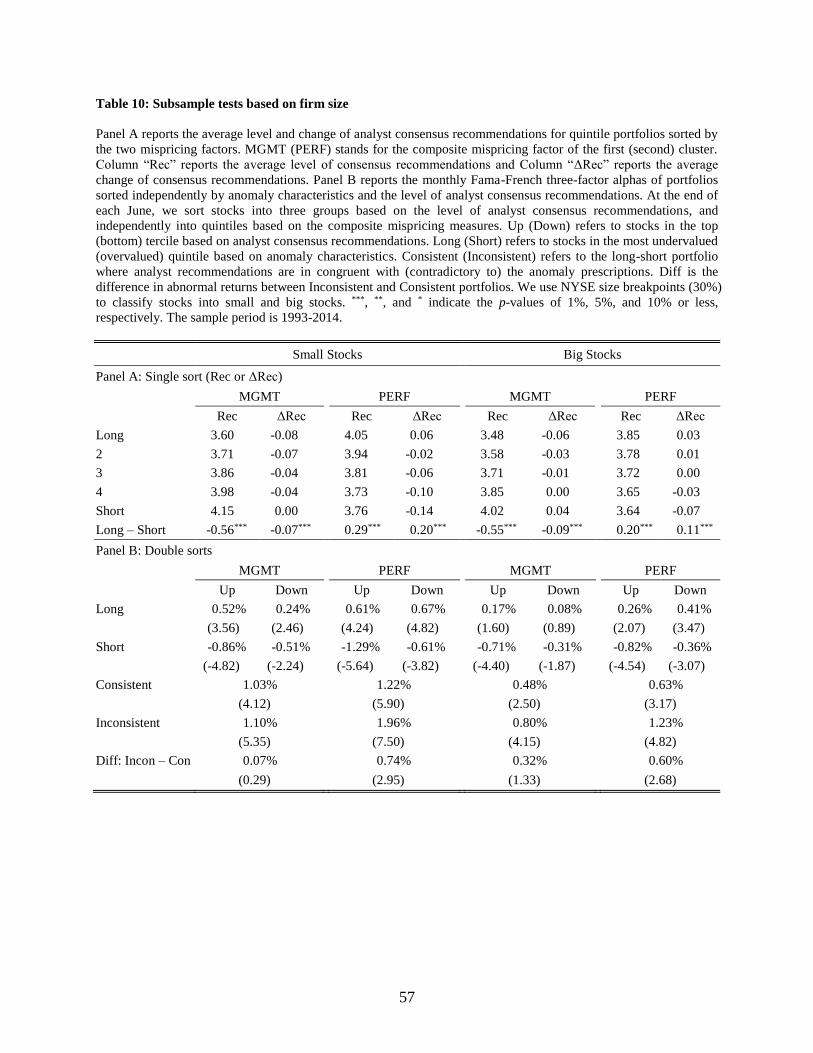
57

Table 10: Subsample tests based on firm size

Panel A reports the average level and change of analyst consensus recommendations for quintile portfolios sorted by

the two mispricing factors. MGMT (PERF) stands for the composite mispricing factor of the first (second) cluster.

Column “Rec” reports the average level of consensus recommendations and Column “ΔRec” reports the average

change of consensus recommendations. Panel B reports the monthly Fama-French three-factor alphas of portfolios

sorted independently by anomaly characteristics and the level of analyst consensus recommendations. At the end of

each June, we sort stocks into three groups based on the level of analyst consensus recommendations, and

independently into quintiles based on the composite mispricing measures. Up (Down) refers to stocks in the top

(bottom) tercile based on analyst consensus recommendations. Long (Short) refers to stocks in the most undervalued

(overvalued) quintile based on anomaly characteristics. Consistent (Inconsistent) refers to the long-short portfolio

where analyst recommendations are in congruent with (contradictory to) the anomaly prescriptions. Diff is the

difference in abnormal returns between Inconsistent and Consistent portfolios. We use NYSE size breakpoints (30%)

to classify stocks into small and big stocks. ***, **, and * indicate the p-values of 1%, 5%, and 10% or less,

respectively. The sample period is 1993-2014.

Small Stocks

Big Stocks

Panel A: Single sort (Rec or ΔRec)

MGMT

PERF

MGMT

PERF

Rec ΔRec

Rec ΔRec

Rec ΔRec

Rec ΔRec

Long 3.60 -0.08

4.05 0.06

3.48 -0.06

3.85 0.03

2 3.71 -0.07

3.94 -0.02

3.58 -0.03

3.78 0.01

3 3.86 -0.04

3.81 -0.06

3.71 -0.01

3.72 0.00

4 3.98 -0.04

3.73 -0.10

3.85 0.00

3.65 -0.03

Short 4.15 0.00

3.76 -0.14

4.02 0.04

3.64 -0.07

Long – Short -0.56*** -0.07*** 0.29*** 0.20*** -0.55*** -0.09***

0.20*** 0.11***

Panel B: Double sorts

MGMT

PERF

MGMT

PERF

Up Down

Up Down

Up Down

Up Down

Long 0.52% 0.24%

0.61% 0.67%

0.17% 0.08%

0.26% 0.41%

(3.56) (2.46)

(4.24) (4.82)

(1.60) (0.89)

(2.07) (3.47)

Short -0.86% -0.51%

-1.29% -0.61%

-0.71% -0.31%

-0.82% -0.36%

(-4.82) (-2.24)

(-5.64) (-3.82)

(-4.40) (-1.87)

(-4.54) (-3.07)

Consistent 1.03%

1.22%

0.48%

0.63%

(4.12)

(5.90)

(2.50)

(3.17)

Inconsistent 1.10%

1.96%

0.80%

1.23%

(5.35)

(7.50)

(4.15)

(4.82)

Diff: Incon – Con 0.07%

0.74%

0.32%

0.60%

(0.29)

(2.95)

(1.33)

(2.68)

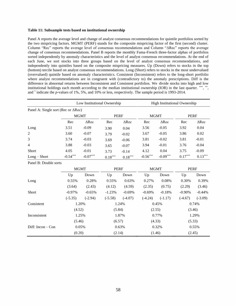
58

Table 11: Subsample tests based on institutional ownership

Panel A reports the average level and change of analyst consensus recommendations for quintile portfolios sorted by

the two mispricing factors. MGMT (PERF) stands for the composite mispricing factor of the first (second) cluster.

Column “Rec” reports the average level of consensus recommendations and Column “ΔRec” reports the average

change of consensus recommendations. Panel B reports the monthly Fama-French three-factor alphas of portfolios

sorted independently by anomaly characteristics and the level of analyst consensus recommendations. At the end of

each June, we sort stocks into three groups based on the level of analyst consensus recommendations, and

independently into quintiles based on the composite mispricing measures. Up (Down) refers to stocks in the top

(bottom) tercile based on analyst consensus recommendations. Long (Short) refers to stocks in the most undervalued

(overvalued) quintile based on anomaly characteristics. Consistent (Inconsistent) refers to the long-short portfolio

where analyst recommendations are in congruent with (contradictory to) the anomaly prescriptions. Diff is the

difference in abnormal returns between Inconsistent and Consistent portfolios. We divide stocks into high and low

institutional holdings each month according to the median institutional ownership (IOR) in the last quarter. ***, **,

and * indicate the p-values of 1%, 5%, and 10% or less, respectively. The sample period is 1993-2014.

Low Institutional Ownership

High Institutional Ownership

Panel A: Single sort (Rec or ΔRec)

MGMT

PERF

MGMT

PERF

Rec ΔRec

Rec ΔRec

Rec ΔRec

Rec ΔRec

Long 3.51 -0.09 3.90 0.04 3.56 -0.05

3.92 0.04

2 3.60 -0.07 3.79 -0.02

3.67 -0.05

3.86 0.02

3 3.74 -0.03 3.69 -0.06

3.81 -0.02

3.81 -0.01

4 3.88 -0.03 3.65 -0.07

3.94 -0.01

3.76 -0.04

Short 4.05 -0.01 3.73 -0.14

4.12 0.04

3.75 -0.09

Long – Short -0.54*** -0.07*** 0.18*** 0.18***

-0.56*** -0.09***

0.17*** 0.13***

Panel B: Double sorts

MGMT

PERF

MGMT

PERF

Up Down

Up Down

Up Down Up Down

Long 0.55% 0.28%

0.55% 0.63%

0.27% 0.08%

0.30% 0.39%

(3.64) (2.43)

(4.12) (4.59)

(2.35) (0.75)

(2.29) (3.46)

Short -0.97% -0.65%

-1.23% -0.69%

-0.69% -0.18%

-0.90% -0.44%

(-5.35) (-2.94)

(-5.58) (-4.07)

(-4.24) (-1.17)

(-4.67) (-3.09)

Consistent 1.20%

1.24%

0.45%

0.74%

(4.52)

(5.84)

(2.55)

(3.46)

Inconsistent 1.25%

1.87%

0.77%

1.29%

(5.46)

(6.57)

(4.33)

(5.33)

Diff: Incon – Con 0.05%

0.63%

0.32%

0.55%

(0.20)

(2.14)

(1.46)

(2.45)

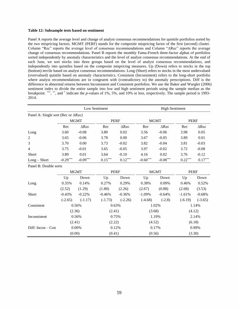
59

Table 12: Subsample tests based on sentiment

Panel A reports the average level and change of analyst consensus recommendations for quintile portfolios sorted by

the two mispricing factors. MGMT (PERF) stands for the composite mispricing factor of the first (second) cluster.

Column “Rec” reports the average level of consensus recommendations and Column “ΔRec” reports the average

change of consensus recommendations. Panel B reports the monthly Fama-French three-factor alphas of portfolios

sorted independently by anomaly characteristics and the level of analyst consensus recommendations. At the end of

each June, we sort stocks into three groups based on the level of analyst consensus recommendations, and

independently into quintiles based on the composite mispricing measures. Up (Down) refers to stocks in the top

(bottom) tercile based on analyst consensus recommendations. Long (Short) refers to stocks in the most undervalued

(overvalued) quintile based on anomaly characteristics. Consistent (Inconsistent) refers to the long-short portfolio

where analyst recommendations are in congruent with (contradictory to) the anomaly prescriptions. Diff is the

difference in abnormal returns between Inconsistent and Consistent portfolios. We use the Baker and Wurgler (2006)

sentiment index to divide the entire sample into low and high sentiment periods using the sample median as the

breakpoint. ***, **, and * indicate the p-values of 1%, 5%, and 10% or less, respectively. The sample period is 1993-

2014.

Low Sentiment

High Sentiment

Panel A: Single sort (Rec or ΔRec)

MGMT

PERF

MGMT

PERF

Rec ΔRec

Rec ΔRec

Rec ΔRec

Rec ΔRec

Long 3.60 -0.08

3.80 0.02

3.56 -0.06

3.98 0.05

2 3.65 -0.06

3.78 0.00

3.67 -0.05

3.89 0.01

3 3.70 0.00

3.73 -0.02

3.82 -0.04

3.81 -0.03

4 3.75 -0.01

3.65 -0.05

3.97 -0.02

3.72 -0.08

Short 3.89 0.01

3.64 -0.10

4.16 0.02

3.76 -0.12

Long – Short -0.29*** -0.09*** 0.15*** 0.12*** -0.60*** -0.08***

0.22*** 0.17***

Panel B: Double sorts

MGMT

PERF

MGMT

PERF

Up Down

Up Down

Up Down

Up Down

Long 0.35% 0.14%

0.27% 0.29%

0.38% 0.09%

0.46% 0.52%

(2.52) (1.29)

(1.80) (2.26)

(2.67) (0.88)

(2.68) (3.53)

Short -0.43% -0.22%

-0.46% -0.36%

-1.09% -0.64%

-1.61% -0.68%

(-2.65) (-1.17)

(-1.73) (-2.26)

(-4.68) (-2.8)

(-6.19) (-3.65)

Consistent 0.56%

0.63%

1.02%

1.14%

(2.36)

(2.41)

(3.68)

(4.12)

Inconsistent 0.56%

0.75%

1.19%

2.14%

(2.41)

(2.22)

(4.52)

(6.18)

Diff: Incon – Con 0.00%

0.12%

0.17%

0.99%

(0.00) (0.41) (0.56)

(3.30)

60

Online Appendix Tables

Table A1: Subsample tests based on trading cost (daily percentage quoted spreads)

Panel A reports the average level and change of analyst consensus recommendations for quintile portfolios sorted by

the two mispricing factors. MGMT (PERF) stands for the composite mispricing factor of the first (second) cluster.

Column “Rec” reports the average level of consensus recommendations and Column “ΔRec” reports the average

change of consensus recommendations. Panel B reports the monthly Fama-French three-factor alphas of portfolios

sorted independently by anomaly characteristics and the level of analyst consensus recommendations. At the end of

each June, we sort stocks into three groups based on the level of analyst consensus recommendations, and

independently into quintiles based on the composite mispricing measures. Up (Down) refers to stocks in the top

(bottom) tercile based on analyst consensus recommendations. Long (Short) refers to stocks in the most undervalued

(overvalued) quintile based on anomaly characteristics. Consistent (Inconsistent) refers to the long-short portfolio

where analyst recommendations are in congruent with (contradictory to) the anomaly prescriptions. Diff is the

difference in abnormal returns between Inconsistent and Consistent portfolios. We divide stocks into high and low

trading cost groups each month, where trading cost is measured by the daily percentage quoted spread following

Chung and Zhang (2014). ***, **, and * indicate the p-values of 1%, 5%, and 10% or less, respectively. The sample

period is 1993-2014.

High Trading Cost

Low Trading Cost

Panel A: Single sort (Rec or ΔRec)

MGMT

PERF

MGMT

PERF

Rec ΔRec

Rec ΔRec

Rec ΔRec

Rec ΔRec

Long 3.60 -0.05

4.05 0.06

3.58 -0.05

4.03 0.05

2 3.71 -0.05

3.95 -0.01

3.69 -0.05

3.92 0.00

3 3.85 -0.04

3.82 -0.05

3.83 -0.03

3.80 -0.04

4 3.98 -0.04

3.73 -0.08

3.96 -0.04

3.73 -0.07

Short 4.15 -0.01

3.77 -0.11

4.13 -0.01

3.73 -0.12

Long – Short -0.56*** -0.04*** 0.28*** 0.17*** -0.55*** -0.03***

0.30*** 0.17***

Panel B: Double sorts

MGMT

PERF

MGMT

PERF

Up Down

Up Down

Up Down

Up Down

Long 0.50% 0.20%

0.58% 0.77%

0.28% 0.14%

0.30% 0.43%

(3.15) (1.82)

(3.82) (5.16)

(2.40) (1.47)

(2.12) (3.86)

Short -0.65% -0.61%

-1.21% -0.77%

-0.83% -0.44%

-0.95% -0.37%

(-3.57) (-2.98)

(-5.58) (-4.87)

(-4.78) (-2.43)

(-4.66) (-2.17)

Consistent 1.11%

1.35%

0.72%

0.67%

(4.53)

(5.89)

(3.29)

(2.71)

Inconsistent 0.85%

1.98%

0.97%

1.38%

(3.99)

(7.46)

(4.76)

(5.08)

Diff: Incon – Con -0.26%

0.62%

0.25%

0.71%

(-0.94) (2.31) (1.03)

(2.92)

61

Table A2: Subsample tests based on long-term institutional ownership

Panel A reports the average level and change of analyst consensus recommendations for quintile portfolios sorted by

the two mispricing factors. MGMT (PERF) stands for the composite mispricing factor of the first (second) cluster.

Column “Rec” reports the average level of consensus recommendations and Column “ΔRec” reports the average

change of consensus recommendations. Panel B reports the monthly Fama-French three-factor alphas of portfolios

sorted independently by anomaly characteristics and the level of analyst consensus recommendations. At the end of

each June, we sort stocks into three groups based on the level of analyst consensus recommendations, and

independently into quintiles based on the composite mispricing measures. Up (Down) refers to stocks in the top

(bottom) tercile based on analyst consensus recommendations. Long (Short) refers to stocks in the most undervalued

(overvalued) quintile based on anomaly characteristics. Consistent (Inconsistent) refers to the long-short portfolio

where analyst recommendations are in congruent with (contradictory to) the anomaly prescriptions. Diff is the

difference in abnormal returns between Inconsistent and Consistent portfolios. We divide stocks into high and low

institutional holdings each month according to the median institutional ownership (IOR) of dedicated institutions in

the last quarter following classification of Bushee (2001) and Bushee and Noe (2000). ***, **, and * indicate the p-

values of 1%, 5%, and 10% or less, respectively. The sample period is 1993-2014.

Low Institutional Ownership

High Institutional Ownership

Panel A: Single sort (Rec or ΔRec)

MGMT

PERF

MGMT

PERF

Rec ΔRec

Rec ΔRec

Rec ΔRec

Rec ΔRec

Long 3.53 -0.06 3.92 0.05 3.54 -0.07

3.90 0.03

2 3.64 -0.04 3.85 0.02

3.66 -0.06

3.85 0.00

3 3.76 -0.01 3.75 -0.02

3.79 -0.04

3.78 -0.03

4 3.91 -0.01 3.68 -0.06

3.92 -0.03

3.73 -0.06

Short 4.08 0.02 3.71 -0.10

4.10 0.02

3.73 -0.12

Long – Short -0.56*** -0.08*** 0.21*** 0.15*** -0.56*** -0.09*** 0.17*** 0.15***

Panel B: Double sorts

MGMT

PERF

MGMT

PERF

Up Down

Up Down

Up Down Up Down

Long 0.54% 0.27%

0.36% 0.41%

0.19% 0.04%

0.36% 0.46%

(3.84) (2.74)

(2.80) (3.54)

(1.63) (0.40)

(2.80) (3.88)

Short -0.96% -0.66%

-1.11% -0.59%

-0.73% -0.16%

-0.98% -0.42%

(-5.64) (-3.15)

(-4.91) (-3.88)

(-4.53) (-0.90)

(-5.06) (-2.95)

Consistent 1.21%

0.95%

0.35%

0.77%

(4.49)

(4.58)

(1.70)

(3.64)

Inconsistent 1.23%

1.53%

0.77%

1.45%

(5.72)

(5.49)

(4.27)

(5.73)

Diff: Incon – Con 0.05%

0.57%

0.42%

0.67%

(0.08) (2.03) (1.82) (2.98)

62

Table A3: Informativeness of six new anomalies

This table reports average returns and alphas on the long-short portfolios of the six new anomalies, including

idiosyncratic volatility (IVOL), max daily return in last month (MaxReturn), past 12-month turnover (Turnover),

cash flow duration (Duration), long-run reversal (LMW), and market beta (Beta) based on the past 5-year estimation

window. Panel A reports the raw returns and Panel B the Fama-French (1993) three-factor alphas. The t-statistics are

in parentheses. The sample period is 1993-2014.

IVOL MaxReturn Turnover Duration LMW Beta

Panel A: Raw returns

Long 0.94% 0.95% 1.04% 1.08% 1.39% 0.65%

(4.06) (4.04) (3.64) (2.87) (2.76) (2.82)

Short 0.35% 0.70% 0.59% 0.88% 0.67% 1.23%

(0.67) (1.11) (1.1) (1.41) (1.63) (1.92)

Long – Short 0.59% 0.25% 0.45% 0.20% 0.72% -0.58%

(1.42) (0.51) (1.29) (0.57) (2.47) (-1.17)

Panel B: Alphas

Long 0.34% 0.36% 0.37% 0.17% 0.30% 0.08%

(3.97) (3.62) (2.54) (1.04) (1.21) (0.80)

Short -0.72% -0.46% -0.53% -0.25% -0.19% -0.05%

(-5.43) (-1.6) (-2.94) (-0.87) (-1.14) (-0.16)

Long – Short 1.06% 0.82% 0.90% 0.42% 0.49% 0.12%

(5.66) (2.65) (4.88) (1.96) (1.82) (0.38)

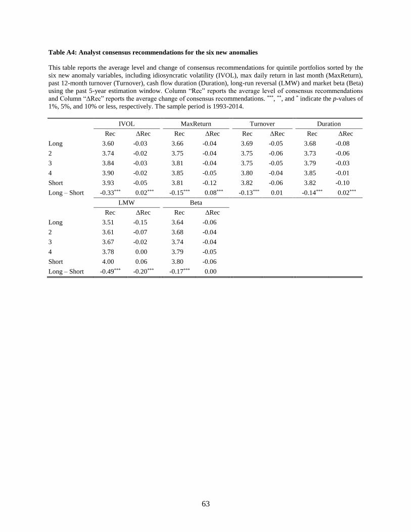
63

Table A4: Analyst consensus recommendations for the six new anomalies

This table reports the average level and change of consensus recommendations for quintile portfolios sorted by the

six new anomaly variables, including idiosyncratic volatility (IVOL), max daily return in last month (MaxReturn),

past 12-month turnover (Turnover), cash flow duration (Duration), long-run reversal (LMW) and market beta (Beta)

using the past 5-year estimation window. Column “Rec” reports the average level of consensus recommendations

and Column “ΔRec” reports the average change of consensus recommendations. ***, **, and * indicate the p-values of

1%, 5%, and 10% or less, respectively. The sample period is 1993-2014.

IVOL

MaxReturn

Turnover

Duration

Rec ΔRec

Rec ΔRec

Rec ΔRec

Rec ΔRec

Long 3.60 -0.03

3.66 -0.04

3.69 -0.05

3.68 -0.08

2 3.74 -0.02

3.75 -0.04

3.75 -0.06

3.73 -0.06

3 3.84 -0.03

3.81 -0.04

3.75 -0.05

3.79 -0.03

4 3.90 -0.02

3.85 -0.05

3.80 -0.04

3.85 -0.01

Short 3.93 -0.05

3.81 -0.12

3.82 -0.06

3.82 -0.10

Long – Short -0.33*** 0.02***

-0.15*** 0.08***

-0.13*** 0.01

-0.14*** 0.02***

LMW

Beta

Rec ΔRec

Rec ΔRec

Long 3.51 -0.15

3.64 -0.06

2 3.61 -0.07

3.68 -0.04

3 3.67 -0.02

3.74 -0.04

4 3.78 0.00

3.79 -0.05

Short 4.00 0.06

3.80 -0.06

Long – Short -0.49*** -0.20***

-0.17*** 0.00

64

Table A5: Abnormal returns of new anomaly portfolios conditional on analyst recommendations

This table reports the monthly Fama-French three-factor alphas of portfolios sorted independently by the six new

anomaly characteristics and the level of analyst consensus recommendations. At the end of each June, we sort stocks

into three groups based on the level of analyst consensus recommendations, and independently into quintiles based

on anomaly characteristics, including idiosyncratic volatility (IVOL), max daily return in last month (MaxReturn),

past 12-month turnover (Turnover), cash flow duration (Duration), long-run reversal (LMW) and market beta (Beta)

using the past 5-year estimation window. Up (Down) refers to stocks in the top (bottom) tercile based on analyst

consensus recommendations. Long (Short) refers to stocks in the most undervalued (overvalued) quintile based on

anomaly characteristics. Consistent (Inconsistent) refers to the long-short portfolio where analyst recommendations

are in congruent with (contradictory to) the anomaly prescriptions. Diff is the difference in abnormal returns

between Inconsistent and Consistent portfolios. The t-statistics are shown in parentheses. The sample period is 1993-

2014.

IVOL

MaxReturn

Turnover

Duration

Up Down

Up Down

Up Down

Up Down

Long 0.42% 0.35%

0.42% 0.36%

0.04% 0.39%

-0.02% 0.32%

(3.93) (3.91)

(3.46) (3.82)

(0.23) (2.94)

(-0.13) (2.09)

Short -0.95% -0.45%

-0.90% -0.08%

-0.77% -0.47%

-0.65% 0.02%

(-6.08) (-2.95)

(-3.20) (-0.24)

(-4.21) (-1.75)

(-2.27) (0.06)

Consistent 0.87%

0.50%

0.51%

-0.05%

(3.94)

(1.36)

(1.95)

(-0.15)

Inconsistent 1.29%

1.26%

1.16%

0.97%

(6.56)

(4.37)

(6.20)

(4.27)

Diff: Incon – Con 0.42%

0.76%

0.64%

1.02%

(2.17)

(3.29)

(2.34)

(3.68)

LMW

Beta

Up Down

Up Down

Long 0.23% 0.30%

0.11% 0.00%

(0.90) (1.09)

(0.92) (-0.01)

Short -0.28% -0.12%

-0.44% 0.23%

(-1.69) (-0.48)

(-1.69) (0.58)

Consistent 0.34%

-0.11%

(1.05)

(-0.27)

Inconsistent 0.58%

0.44%

(1.98)

(1.62)

Diff: Incon – Con 0.24%

0.55%

(0.86)

(2.02)

65

Table A6: Unconditional Return Predictability of Consensus Analyst Recommendations

This table reports the monthly Fama-French three-factor alphas of quintile portfolios sorted on consensus analyst

recommendations. At the beginning of every quarter (month), we sort stocks into quintiles based on the level or

change of recommendations observed at the last quarter (month) end, and re-balance the portfolio quarterly

(monthly). Panel A (B) reports the results for quarterly (monthly) re-balanced portfolios and t-statistics are reported

for the long minus short portfolios.

Panel A: Quarterly rebalanced portfolios

1993-2000

2000 - 2007

2008 - 2014

1993 - 2014

Rec ΔRec

Rec ΔRec

Rec ΔRec

Rec ΔRec

Short 0.46% 0.60%

1.00% 0.74%

0.94% 1.10%

0.80% 0.82%

2 0.76% 1.10%

0.83% 0.99%

1.06% 0.94%

0.88% 1.01%

3 0.88% 0.91%

1.04% 0.80%

1.09% 1.02%

1.00% 0.91%

4 0.40% 0.94%

0.55% 0.83%

0.92% 1.05%

0.62% 0.94%

Long 0.31% 1.02%

0.56% 0.85%

0.82% 1.07%

0.56% 0.98%

Long – Short -0.14% 0.43%

-0.44% 0.11%

-0.12% -0.03%

-0.23% 0.16%

t-stat (-1.27) (2.17) (-1.32) (0.53) (-1.47) (-0.31) (-1.64) (1.76)

Panel B: Monthly rebalanced portfolios

1993-2000

2000 - 2007

2008 - 2014

1993 - 2014

Rec ΔRec

Rec ΔRec

Rec ΔRec

Rec ΔRec

Short 0.46% 0.48%

1.01% 0.74%

0.93% 1.01%

0.80% 0.76%

2 0.68% 1.00%

0.71% 0.92%

1.03% 0.95%

0.81% 0.96%

3 0.90% 0.96%

1.13% 0.80%

1.08% 1.03%

1.03% 0.93%

4 0.46% 0.79%

0.58% 0.83%

0.96% 1.04%

0.66% 0.89%

Long 0.52% 1.17%

0.64% 0.87%

0.86% 1.18%

0.67% 1.07%

Long – Short 0.06% 0.69%

-0.37% 0.13%

-0.06% 0.16%

-0.13% 0.31%

t-stat (-0.34) (2.79) (-0.99) (0.59) (-1.16) (0.67) (-0.77) (2.85)