SeDFAM: Semiconductor Demand Forecast Accuracy Model

Metin Cakanyıldırım

School of Management, University of Texas at Dallas, Richardson, Texas 75080.

Robin O. Roundy

Operations Research and Industrial Engineering, Cornell University, Ithaca, New York 14850.

Abstract

In the semiconductor industry, many critical decisions are based on demand forecasts. However,

these forecasts are subject to random error. In this paper, we lay out a scheme estimating the vari-

ance and correlation of forecast errors (without altering given forecasts) and modeling the evolution

of forecasts over time. Our scheme allows correlations across time, products and technologies. It

also addresses the case of nonstationary errors due to ramps (technology migrations). It can be used

to simulate chip demands for production planning / capacity expansion studies.

1 Introduction

In this paper, we will attempt to quantify forecast errors, i.e., the differences between forecasts and actual demands

for semiconductors. Some of the most important, difficult and risky decisions made by semiconductor companies are

based on demand forecasts. Capacity acquisition and deployment are prime examples. Cakanyıldırım and Roundy

[1] mentions that a semiconductor machine costs around $1-3M while a fab costs $1-2B. Because of long machine

delivery lead times, capacity acquisition decisions must be made well in advance with inaccurate demand forecasts.

Our primary goal is to quantify the risks associated with capacity acquisition decisions, and with a variety of other

forecast-based decisions.

We take a set of current and historical demand forecasts, model the forecast error as a vector-valued random

variable, estimate its distribution, and randomly generate possible futures with minimal user input. However, totally

autonomous generation of forecasts is outside the scope of this study. Semiconductor demand forecasting is a complex

process. In this process, forecasters use many sources of information. The process is difficult to quantify and represent

mathematically. Therefore, we do not propose an alternative forecasting scheme.

The study of forecast quality is particularly relevant for the semiconductor industry because high volatility makes

forecasting challenging. Moreover, it is believed in the industry that forecast accuracy is getting worse, both because

product life cycles are shortening and because line-widths are shrinking (see [1]). Line-width shrinkage often makes

it harder to sell chips produced under an old technology with wider widths unless substantial discounts are made.

Thus, demand for a certain line-width of a certain product often resembles that of a style good which will not be

demanded after a certain point in time.

Within the context of forecasting, semiconductor product families can be divided roughly into two groups. Families

in the first group have persistent demand over extended periods of time, such as memory, ASICS, CPUs, controller

chips for desktop printers, etc. As time advances these families evolve, and they are migrated to finer and finer line

widths, but the overall demand for the product family continues. For these product families, the requirements for

manufacturing capacity is a function of overall family demand, of line width migrations, and of a variety of other

technological factors, all of which need to be forecasted.

1

Product families in the second group are just coming into existence, and consequently have no historical data

that can be used in forecasting. For these families methodologies that were developed for style goods and by Meixell

and Wu [2] are applicable. This paper focuses on semiconductor families that have persistent demand over extended

periods of time.

A primary concern will be the evolution of forecasts as time passes. Consider forecasts of domestic PC sales in

December 2000. We start forecasting at the beginning of January 2000 and update the forecast every month. At the

beginning of December 2000, we will have produced 12 forecasts for December sales. Actual sales can be thought

as a forecast with zero error. Putting these 13 numbers into chronological order we see how forecasts for December

sales evolve over time from a highly uncertain forecast in January to a sharply accurate one in December.

2 Literature Survey

There is a huge time-series literature on methods to generate demand forecasts (see Hamilton [3]). Since we

investigate forecast errors for a style good (semiconductors) as opposed to forecast generation, we mention a few,

relatively recent, papers that study forecasting, especially for new products or style goods. Mahajan and Wind

[4] survey the new product forecasting models. Murray and Silver [5] represent the demand of a style good as

a binomial random variable where the number of potential buyers is constant but the probability of a customer

purchase is updated using past sales. Chang and Fyffe [6] visualize monthly demands as a fixed fraction of the total

demand for a style good. Total demands are modified as monthly sales are revealed.

In forecasting new product demands, the Bass function [7] is often used. Norton and Bass [8] model diffusion

of a new product (demand migration) in the markets. Kurawarwala and Matsuo [9] study seasonal PC demands.

In both models parameters of the Bass function are updated periodically.

Another stream studies forecast revisions with partially observed (demand) data. The main driving idea in

Guerrero and Elizondo [10], Kekre et al. [11], and Bodily and Freeland [12] is presuming that the forecasted

quantity is revealed in steps (over time). Moreover, partial observations can be used to forecast the whole quantity.

For example, in one of the models it is assumed that the ratio of orders received up to a certain time to the whole

2

demand is approximately constant. After the proportionality constant is estimated, forecasts are readily generated

from the partially observed demands.

A relatively early example of updating forecasts in a Bayesian manner is Azoury [13]. It assumes that demand

has a particular density and updates parameters of that density by conditioning on previous demands. The idea

of updating forecasts in a Bayesian fashion through leading indicator products is introduced by Meixell and Wu in

[2]. In this scheme, forecaster observes the demand for a particular product and revises forecasts for other products

whose demands are strongly correlated with those of the particular product. For new products, and for products that

are being phased out, the general approaches that have been developed within this scheme, and those for style good

forecasting, are applicable. The scheme developed by Meixell and Wu outputs demand scenarios instead of forecasts,

thus it constitutes an example of the contemporary practice of forecasting with scenarios argued by Bunn and Salo

[14]. Angelus et al. [15] ties the current period’s demand to the last period’s demand through a random multiplier

whose expected value is greater than one. Works of Meixell and Wu, and Angelus are done on semiconductor demands

and so are particularly relevant. However, they primarily aim to generate demand scenarios/forecasts whereas our

primary goal is to evaluate the quality of the forecasts.

As far as we know, the first work that attempted to understand the evolution of forecasts is Hausman [16]. For

some real life data sets, he statistically validates the hypothesis that ratios of successive forecasts are Lognormal

variates. Graves, Meal, Dasu and Qui [17] treats the forecasting process as a black box and study forecast variances.

However, [17] assumes that forecasts are serially independent. Heath and Jackson [18], unaware of [17], propose a

more general model allowing serial dependence and estimate the covariance matrix of stationary demand forecasts.

That matrix is also used to simulate demand forecasts. In recent studies, Gullu [19] and Toktay [20] have investigated

the value of incorporating this technique into production planning and inventory holding, respectively. Graves, Kletter

and Hetzel [21] also use Heath-Jackson framework to study production smoothing and safety stock holding tradeoffs.

They show how to linearly convert forecast updates into production schedule updates so that a measure of production

smoothing is minimized subject to an upper bound on a measure of safety stock.

We focus on semiconductor product families that have persistent demand over extended periods of time, but which

are affected by successive waves of technological innovation and improvement. The level of detail in our models is

3

driven by a desire to support the acquisition of manufacturing capacity, and related decisions. At this level of detail

demands become nonstationary with technology improvements. We propose a forecast evolution model that handles

nonstationarity and that is a result of ideas blended from Heath-Jackson framework and style goods forecasting. Our

primary goal is the estimation of variances and covariances of forecast errors affecting different products in different

time periods. We have also created a tool that can be used to simulate the manner in which forecasts evolve.

3 Fractional and Perceived Age Forecasts

In this section we present two concepts, fractional forecasts and perceived age forecasts. We also discuss the role

that these forecasts play in our forecast error estimation procedure.

We group part numbers into product families at the highest level and into products at a finer level. Chips belonging

to the same functional category are put into the same product family. For example memory chips constitute a product

family. Chips of the same product family are further grouped according to technology (e.g. CMOS 12). Let p and

tec denote a generic product family and a technology respectively. The product family p and the technology tec

define a product (p, tec) uniquely. An example of a product defined as such is (Memory,CMOS 12).

In the semiconductor industry, within each product family, demand for a given technology dies out and is replaced

by demand for a newer technology. We call this process migration of product families. The S-curve (p, tec) represents

forecasted demand for the family p and for the technology tec plus demands for all technologies newer than tec.

In Figure 1, a piece of the S-curve (Memory,CMOS 8), and S-curves (Memory,CMOS 10) and (Memory,CMOS 12)

are shown. Due to migration of product families, one often expects those curves to be nondecreasing. The vertical

distances between consecutive S-curves is the demand for memory chips with a single technology.

In addition to working with absolute quantities on the vertical axis of Figure 1, the ratio of those absolute figures

to the total product family demand will be of interest. Let dp,tecs,t be the demand of product family p and technology

tec, forecasted from period s for period t. From now on, we use the phrase from s for t to refer to forecasts made in

period s for demands to be realized in period t. When s = t, the quantity in question is no longer a forecast but an

actual demand. For practical reasons, in each period s forecasts are made only for the next H periods: s+1,...,s+H.

4

We refer to H as the forecast horizon. Let cdp,tecs,t be the (cumulative) demand for all technologies newer than or

equal to tec of family p, from s for t. Furthermore define dps,t, the forecast for family p, and fp,tec

s,t , the fractional

forecast, as

dps,t =

∑

tec

dp,tecs,t

cdp,tecos,t =

∑

tec is tec0 or newer

dp,tecs,t

fp,tecs,t =

cdp,tecs,t

dps,t

. (1)

Note that 0 ≤ fp,tecs,t ≤ 1, and that fp,tec

s,t can be easily calculated from the demand forecast data.

We summarize commonly used notation in Appendix A. For simplicity we discuss family demands with no trend

or seasonality. For the case where trend or seasonality are present see Appendix B.

Recall that we are dealing with the demand forecasts for products that correspond to various technologies within

existing product families rather than demand forecasts for new product families. For such products and product

families, partly due to product compatibility the relationship between a semiconductor manufacturer and an OEM

tends to be more stable than many other aspects of the consumer electronics business. Therefore, the market (exterior

forces) is the primary driver for family demands dpt,t. Contrary to that, the company’s technology (interior forces)

mostly drives fractional demands fp,tect,t . This idea is embodied in the first of the following independence assumptions.

(I1): Product family demands and fractional demands are independent. Meixell and Wu [2] (see section II.A.2)

also make a similar assumption. For a formal statement of the assumption see (9).

(I2): Random variables which we observe as fp,tec1s,t and fp,tec2

s,t are independent for tec1 6= tec2. In other words

shifts in different S-curves of Figure 1 are independent. For a formal statement see (10).

An example will clarify and motivate Assumption (I2). Let A, B denote the fractional demands for technologies

8 and 10 of the same product family at a particular time, respectively. Then the fractional cumulative demands

are A+B, and B for 8 and 10, respectively. If the forecast for B increases (corresponding to faster migration than

estimated), then the forecast for A will probably decrease, because demand for B will replace demand for A. However,

it is not clear how A+B will behave. In practice one might expect A and A+B to have some degree of correlation.

5

However, there is no indication of significant correlations (between different ramps) either in our interviews with

people in the semiconductor industry (see [1]) or in the industrial data we have.

When using (1) in practice a word of caution is in order. Wafers are a common unit of measure for semiconductor

products. However, if a new memory chip stores more data per wafer and there is a constant demand for data

storage, demand for wafers will go down. When aggregating data, units should be chosen to minimize the impact of

technology changes on total family demand.

Suppose that fp,tecs,t = 0.4 and fp′,tec′

s,t = 0.98. In period s + 1 these forecasts will be updated by amounts,

a = fp,tecs+1,t − fp,tec

s,t and a′ = fp′,tec′s+1,t − fp′,tec′

s,t . But a is likely to be larger in absolute value than a′ because fp′,tec′s,t

is very close to its maximum value 1. To eliminate this effect we transform fractional forecasts into perceived age

forecasts. Let L be the average length of a technology ramp, i.e. the average length of the S-curves in Figure 1. We

use the phrase age of a ramp to refer to the duration between the start of the ramp and the current time. Define

a nondecreasing ramp function R : [0, L] → [0, 1], which maps the age of a typical ramp to the fraction of product

family demand achieved. R is obtained by fitting a curve to all the S-curves available in the historical database while

requiring R(0) = 0 and R(L) = 1. We extend the domain of R to (−∞,∞) by defining R(δ) = 0 if δ ≤ 0, and

R(δ) = 1 if δ ≥ L. Let δp,tecs,t be the perceived age forecast from s for t, where

δp,tecs,t = R−1(fp,tec

s,t ). (2)

δp,tecs,t is different from the actual age of the ramp. If R−1(0.3) = 6 then in a “typical” ramp, 30% of the family demand

shifts to the new technology 6 months after the beginning of the ramp. If δp,tecs,t = 6 (or equivalently fp,tec

s,t = 0.3),

then according to the period s forecast, at time t the (p, tec) ramp will be at the 30% level. If the ramp up during

period t is forecasted to be faster (slower) than usual, then δp,tecs,t+1 > δp,tec

s,t + 1 (δp,tecs,t+1 < δp,tec

s,t + 1).

Forecast evolution studies the incremental transition of forecasts as time advances. We will now define some

statistics that capture the mechanism of forecast evolution.

To illustrate the concept of forecast evolution, note that the family demand forecast dps−1,t, the fractional forecast

fp,tecs−1,t and the perceived ramp age forecast δp,tec

s−1,t are all generated at time s−1. During period s−1 more information

is obtained. Consequently, in period s the forecaster produces revised forecasts dps,t, fp,tec

s,t and δp,tecs,t . Updates on

6

perceived ramp ages δp,tecs,t and product family demands dp

s,t are denoted with up,tecs,t with vp

s,t. These are calculated

as

vps,t = dp

s,t − dps−1,t and

up,tecs,t = δp,tec

s,t − δp,tecs−1,t = R−1(fp,tec

s,t )− R−1(fp,tecs−1,t). (3)

At every time period s, an update vector vs for family demand forecasts will be constructed as

vs = [vX86s,s , ..., vX86

s,s+H−1, vMems,s , ..., vPPC

s,s , ..]

where X86, Memory, PPC are typical product families in the semiconductor industry. The perceived age update

vector utecs is similar, but more intricate. At every time period s, an update vector for a currently ramping technology

will be constructed by putting all updates (H updates for each product family) into a vector utecs . For example,

assume that memory and X86 are the only two product families. At time s, we create two vectors u8s and u10

s , one

for technology 8 and one for technology 10 as follows

u8s = [uX86,8

s,s , ..., uX86,8s,s+H−1, u

Mem,8s,s , ..., uMem,8

s,s+H−1] u10s = [uX86,10

s,s , ..., uX86,10s,s+H−1, u

Mem,10s,s , ..., uMem,10

s,s+H−1]. (4)

This specific construction lets us observe several update vectors (one for each active technology) in a single period.

Different technologies are not put into the same update vector because they are assumed to be independent (see

(I2)). In general, utecs has entries for each product p and each t, s ≤ t < s + H.

However, with the above construction, not all components of a given update vector will be observed in all periods.

If tec = 10 is introduced into family X86 at time t, then no perceived age forecast δX86,10s,∗ will be available in period

s = t−H − 1. Two periods later in period t−H + 1, the update vector u10t−H+1 will have a single observed element,

uX86,10t−H+1,t. In the next period, the update vector u10

t−H+2 will have two observed elements, and so forth. At a given

point in time a particular technology may be used for some product families, but not for the others. In that case,

only forecast updates of product families using that technology will be observed. Many (or most) of the update

vectors will have missing data. This will affect our estimation procedures.

We will finish this section by introducing a procedure called SeDFAM (acronym for Semiconductor Demand

Forecast Accuracy Model). SeDFAM uses historical and current forecasts to estimate variances and covariances of

7

Computation See Section

Inputs : Historical Demand forecasts, dp,tecs,t , for all s, t, s ≤ t ≤ s + H. 3

1. Compute historical family forecasts dps,t and fractional forecasts fp,tec

s,t . Use (1). 3

2. Fit ramp function R to historical ramps. See the paragraph before (2). 3

3. Compute perceived age forecasts δp,tecs,t = R−1(fp,tec

s,t ); see (2). 3

4. Compute family forecast updates vps,t = dp

s,t − dps−1,t; see (3). 3

5. Compute perceived age forecast updates up,tecs,t = δp,tec

s,t − δp,tecs−1,t; see (3). 3

6. Estimate family forecast update covariance matrix, Λ. Use standard statistical techniques. 4

7. Estimate perceived age forecast update covariance matrix, Σ. Use the EM algorithm. 4

8. Use R , Λ , Σ to compute variances and covariances of demands as seen in period now. 5

Use the Monte-Carlo approach described in Section 5.

Table 1: Steps of the SeDFAM

future demands. Table 1 summarizes the computations required by SeDFAM. In this section we have discussed steps

1-5.

Section 4 uses the language of random variables to describe update vectors. We also estimate the covariance

matrices for update vectors (steps 6 and 7) in Section 4. In Section 5 we complete our definition of SeDFAM by

laying out the Monte-Carlo approach used to compute variances and covariances of future demands based on current

and historical forecasts. This corresponds to step 8 in Table 1.

4 A Probabilistic Model for Forecast Evolution

In this section, we provide a probabilistic model for forecast evolution and describe steps 6 and 7 of SeDFAM. From

now on we will use capital letters for random variables and small letters for observations from those random variables.

We will focus our discussion on the evolution of perceived ramp age forecasts δs,t. The evolution of product family

demand forecasts is treated exactly the same way: it suffices to replace δp,tecs,t (∆p,tec

s,t ) with dps,t (Dp

s,t) and up,tecs,t

8

(U tecs ) with vp

s,t (Vs) in the current section. Assumptions we make in this section, (A1-3) and (I3), apply to updates

on both product family forecasts and perceived ramp age forecasts.

Let =r be the information available at time r (=r stands for the σ − field at time r). We will use notation

inspired from conditioning to distinguish between the versions of the forecasts as seen from different time periods.

Specifically, Dp,tecs,t |=r, F p,tec

s,t |=r, ∆p,tecs,t |=r and Up,tec

s,t |=r refer to the random variables corresponding to dp,tecs,t fp,tec

s,t ,

δp,tecs,t and up,tec

s,t , as seen from period r. Thus, F p,tecs,t |=r, ∆p,tec

s,t |=r and Up,tecs,t |=r are all random for r < s, but

fp,tecs,t = F p,tec

s,t |=s, δp,tecs,t = ∆p,tec

s,t |=s and up,tecs,t = Up,tec

s,t |=s are deterministic.

We describe semiconductor demand forecasts using a hierarchy of random variables based on (1), (2) and (3). In

Figure 2 the dependence on the information set is suppressed. Thus we write Dps,t for Dp

s,t|=r, etc. The matrices Λ

and Σ of Figure 2 are defined in Assumption (I3) below.

The stochastic version of equation (3) is

Up,tecs,t |=r = (∆p,tec

s,t −∆p,tecs−1,t)|=r. (5)

Following Heath and Jackson [18], we make the following assumptions on the update random variable:

(A1) No Learning: Nothing is learned about Up,tecs,t before period s. Up,tec

s,t indeed represents the additional information

learned in period s. For r < s, all Up,tecs,t |=r have the same distribution as the generic random variable Up,tec

s,t :=

Up,tecs,t |=s−1. No Learning implies that Up,tec

s,t and Up,tecr,w are uncorrelated for s 6= r.

(A2) Stationarity: Up,tecs,t = Up,tec

s+h,t+h in distribution for any increment h.

(A3) Zero Expected Value: E(Up,tecs,t ) = 0. Appendix C discusses how to proceed when this assumption fails.

As we mentioned earlier, we defined perceived ramp age forecasts so that (A2) becomes a reasonable assumption.

Fractional updates (fp,tecs,t − fp,tec

s−1,t) tend to be smaller when fp,tecs,t is close to either 0 or 1, so fractional updates

depend on ramp ages. Up,tecs,t is called a normalized update because its distribution depends on the difference between

t and s (by (A2)), but not on t, s or the ramp age.

We now discuss the algebra relating forecast updates to forecasts. Forecasts made for periods too far into the

future are not useful, so we have a finite forecast horizon H. Thus, perceived age forecasts ∆p,tecs,t |=r for s < t −H

will not be defined. Before period t − H + 1, the only information available on period t demand is δp,tect−H,t, so for

9

r ≤ t − H ≤ s, ∆p,tecs,t |=r = ∆p,tec

s,t |=t−H and ∆p,tect−H,t|=r = δp,tec

t−H,t. Then it follows via (5) that the perceived age

forecast is

∆p,tecs,t |=r = ∆p,tec

s,t |=t−H = δp,tect−H,t +

s∑

j=t−H+1

Up,tecj,t |=t−H r ≤ t−H ≤ s ≤ t. (6)

Note that ∆p,tecs,t |=r does not evolve with r for r ≤ t−H. The case of r ≥ t−H is more interesting. In general, from

Equation (5)

∆p,tecs,t |=r = δp,tec

(r∧s)∨(t−H),t +s

∑

j=[(r∧s)∨(t−H)]+1

Up,tecj,t |=r∨(t−H)

= δp,tect−H,t +

(r∧s)∨(t−H)∑

j=t−H+1

up,tecj,t +

s∑

j=[(r∧s)∨(t−H)]+1

Up,tecj,t , t−H ≤ s ≤ t (7)

where r ∧ s = min(r, s) and r ∨ s = max(r, s). The second equality follows from the assumption of No Learning

about updates Up,tecj,t before they are observed. Indeed, (7) generalizes (6), i.e., it holds for any value of r as long as

t−H ≤ s ≤ t. As r increases, the deterministic component of perceived age forecasts (for fixed s and t) grows, and

the forecast eventually becomes deterministic at r = s (δp,tecs,t = ∆p,tec

s,t |=s). It follows from Equation (7) that the

stochastic parts of ∆p,tecs,t |=r and ∆p,tec

s+h,t+h|=r+h have the same distribution for any increment h.

Obtaining forecasts via Equation (7) has a nice feature. The mean square error of perceived age forecasts is

non-increasing and goes to zero as s approaches t for any r, i.e.,

E[(∆p,tect,t −∆p,tec

s,t )2|=r] =t

∑

j=(s∨r)+1

var(Up,tecj,t ) + {

r∧t∑

j=(s∧r)+1

up,tecj,t }2.

The last equality follows from the No Learning assumption and the Zero Expected Value assumption.

Perceived age forecasts are unbiased if (A3) holds. Unbiasedness indicate that an observation δp,tecs,t is equal to

the expected value of ∆p,tect,t where the expectation is taken relative to information available in period s. Although

∆p,tecs,t |=r and ∆p,tec

s,t |=r+1 have different means, perceived age forecasts as given by equation (7) satisfy

E(∆p,tect,t |=s) = ∆p,tec

s,t |=s = δp,tecs,t . (8)

Thus, as a consequence of the No Learning and Zero Expected Value assumptions, perceived age forecasts are unbiased.

When forecasts are made from s for t (where s ≤ t), we coin the term (forecast) lag for t−s. We say that δp,tecs,t (dp

s,t)

is a lag biased forecast if E(Up,tecs,t ) (E(V p

s,t)) differs from zero by a deterministic function of the lag. In Appendix C,

we illustrate how our work can be extended to accommodate lag bias.

10

Fractional forecasts are related to perceived age forecasts via a nonlinear ramp curve R (see Equation (2)).

Perceived age forecasts are unbiased by (8) but, there will be bias in fractional forecasts F p,tecs,t . That is because R

is a nonlinear function, so E(F p,tect,t |=s) = E(R(∆p,tec

t,t )|=s) 6= R(E(∆p,tect,t |=s)) = fp,tec

s,t . In regions where the ramp

function is approximately linear, this nonlinearity-induced bias will be small. We will revisit the magnitude of the

bias in the numerical experiments section.

Perceived age forecasts constitute a martingale, i.e. E(∆p,tecs,t |=r) = δp,tec

r,t if t − H ≤ r ≤ s ≤ t. Perceived age

forecasts could be constructed as conditional expectations, i.e. we could define δp,tecs,t = E(∆p,tec

t,t |=s). We could also

define δp,tecs,t as a minimum mean-squared error forecast. These approaches are discussed in Brockwell and Davis

[22], and Heath and Jackson [18].

Now we are in a position to give formal statements of our first two independence assumptions.

(I1) : U tecs and Vs are independent for all s and tec. (9)

(I2) : U tec1s and U tec2

s are independent if tec1 6= tec2. (10)

For convenience, we assume normality of update vectors:

(I3): U tecs is normally distributed with covariance matrix Σ for all (s, tec).

Vs is normally distributed with covariance matrix Λ for all s.

Assumptions (A1), (A3), (I2) and (I3) imply that update vectors U tecs are i.i.d., distributed as U ∼ N(0,Σ). If

s1 6= s2, independence of U tec1s1

and U tec2s2

is a consequence of (A1) and (I3). If tec1 6= tec2, it is a restatement of (I2).

However, the components of the vector U tecs will be dependent among themselves. Thus, we still capture demand

correlations among different product families as well as among time periods. We make assumptions analogous to

(A1)-(A3) and (I3) to deduce that family forecast update vectors, Vs are normally distributed as V ∼ N(0, Λ). For

a full characterization of our update vectors U tecs and Vs, it suffices to estimate Σ and Λ.

Step 6 of SeDFAM, the estimation of the covariance matrix Λ for the update vector Vs is straightforward because

the vector Vs has no missing elements. See Anderson [23] for details.

We now discuss the step 7 of SeDFAM, the estimation of Σ, the covariance matrix for perceived age updates.

Estimation will be based on a maximum likelihood framework. We number the vectors utecs from 1 to N , to obtain

11

the sample {ui : i = 1..N}. N is approximately the number of time periods times the average number of active

technologies produced at a given time. The MLE estimator Σ of the covariance matrix Σ solves the following problem:

minΣN2

log|Σ| +12

N∑

i=1

uiΣ−1uTi .

The solution to this minimization problem is easily found when no data is missing (see [23]). Since the vectors U tecs

have missing data, we use an iterative procedure called the EM algorithm for maximizing the likelihood function

given the observed data. The EM algorithm has both a Frequentist and a Bayesian version. Details of the EM

algorithm are found in Schafer [24]. When it converges, we recommend the Frequentist version because of the

difficulty of obtaining appropriate priors (see Section 8.2).

5 Estimating Demand Covariances via Simulations of Future

Before describing the final step of SeDFAM, we describe a procedure for simulating future realizations of demands

and forecasts, given current and historical forecasts. This capacity can be used to quantify the risk associated with

a business decision. It can drive simulations of fabs, of supply chains, etc. It can also be used to automatically

generate scenarios for stochastic optimization algorithms.

Having completed steps 1-7 of SeDFAM, we use Monte-Carlo simulation to generate a set of future forecasts

for period t, now < t ≤ now + N , where now is the current time period and N denotes the number of periods

beyond now whose forecasts are of interest. Note that when s = t forecasts are actual demands. We assume that for

future periods t, now + H < t ≤ now + N , dp,tect−H,t are exogenously generated. Let τt = now ∨ (t −H). Thus δp,tec

τt,t

and dpτt,t are given for all t, now < t ≤ now + N , - being taken from the current forecasts if τt = now, and being

computed from dp,tect−H,t if τt = t−H > now. Noting that not all technologies are used in all time periods, we define

Π := {(t, p, tec) : now < t ≤ now + N , δp,tecτt,t exists}.

We use δp,tecs,t to refer to an observation drawn from the random variate ∆p,tec

s,t |=now, with up,tecs,t , vp

s,t, fp,tecs,t , dp

s,t

and dp,tecs,t being similarly defined. Table 2 contains our Forecast Simulator. Note that it follows the hierarchical

structure in Figure 2.

The Forecast Simulator algorithm generates future forecasts [dp,tecs,t : (t, p, tec) ∈ Π , τt < s ≤ t], a random

12

1. Generate update vectors. utect and vt for all (t, tec) such that (t, p, tec) ∈ Π for some p. utec

t and

vt are drawn from N(0, Σ) and N(0, Λ).

2. Compute future family, perceived age and fractional forecasts: Following (7) and (2) we obtain

forecasts for period t as

δp,tecs,t = δp,tec

τt,t +∑s

j=τt+1 up,tecj,t , (t, p, tec) ∈ Π , τt < s ≤ t

dps,t = dp

τt,t +∑s

j=τt+1 vpj,t , (t, p, tec) ∈ Π for some tec , τt < s ≤ t.

fp,tecs,t = R(δp,tec

s,t |=now) , (t, p, tec) ∈ Π , τt < s ≤ t

3. Generate future product demands: By the definition of fractional forecasts in (1), we obtain

product forecasts for period t by combining product family and fractional forecasts:

dp,tecs,t = (dp

s,t)(fp,tecs,t − fp,tec+

s,t ) , (t, p, tec) ∈ Π , τt < s ≤ t

Table 2: Steps of Forecast Simulator.

instance drawn from [Dp,tecs,t |=now : (t, p, tec) ∈ Π , τt < s ≤ t]. The algorithm can be executed for K times to

generate an independent and identically distributed (iid) sample of K random instances of [Dp,tecs,t |=now : (t, p, tec) ∈

Π , τt < s ≤ t]. If future demands are of interest but future forecasts are not, steps 2 and 3 can be limited to s = t.

The final step of SeDFAM is to compute the covariance matrix of [Dp,tect,t |=now : (t, p, tec) ∈ Π], where N = H.

We accomplish this by setting N = H, s = t and executing the Forecast Simulator K times to obtain a sample of

iid instances [dp,tecs,t : (t, p, tec) ∈ Π] of [Dp,tec

t,t |=now : (t, p, tec) ∈ Π]. We then compute the sample variance matrix in

the classical manner.

We could calculate the variances and covariances analytically in Step 8 of SeDFAM. From (1), we obtain:

Dp,tect,t |=now = {Dp

t,t|=now}{(F p,tect,t |=now)− (F p,tec+

t,t |=now)} (11)

where tec stands for a technology and tec+ denotes the next technology introduced after tec. We suppress =now in

the notation for brevity. From the independence of product family and fractional demands, we obtain

13

Cov(Dp1,tec1t1,t1 , Dp2,tec2

t2,t2 ) = Cov(F p1,tec1t1,t1 − F p1,tec1+

t1,t1 , F p2,tec2t2,t2 − F p2,tec2+

t2,t2 )E(Dp1t1,t1D

p2t2,t2)

+ Cov(Dp1t1,t1 , D

p2t2,t2)E(F p1,tec1

t1,t1 − F p1,tec1+t1,t1 )E(F p2,tec2

t2,t2 − F p2,tec2+t2,t2 ).

(12)

Cov(F p1,tec1t1,t1 −F p1,tec1+

t1,t1 , F p2,tec2t2,t2 −F p2,tec2+

t2,t2 ) is the most interesting term. This covariance is zero if tec2 comes after

tec1+. Suppose tec = tec2 = tec1. Using the independence of different technologies,

Cov(F p1,tect1,t1 − F p1,tec+

t1,t1 , F p2,tect2,t2 − F p2,tec+

t2,t2 ) = Cov(R(∆p1,tect1,t1 ), R(∆p2,tec

t2,t2 )) + Cov(R(∆p1,tec+t1,t1 ), R(∆p2,tec+

t2,t2 )). (13)

Note that the vector

[∆p1,tect1,t1 , ∆p2,tec

t2,t2 , ∆p1,tec+t1,t1 , ∆p2,tec+

t2,t2 ] (14)

is normally distributed with expected value [δp1,tecr,t1 , δp2,tec

r,t2 , δp1,tec+r,t1 , δp2,tec+

r,t2 ].

The covariance matrix of this vector can be expressed in terms of Σ using (7). Having done so, computing the

covariance in (13) requires 2-dimensional numerical integrations. Such integrations become tedious when R is a

piece-wise quadratic spline function, as in our numerical experiments. Thus, we prefer Monte-Carlo procedure. With

this description of step 8, we complete our definition of SeDFAM.

6 Studying a Base Case with SeDFAM

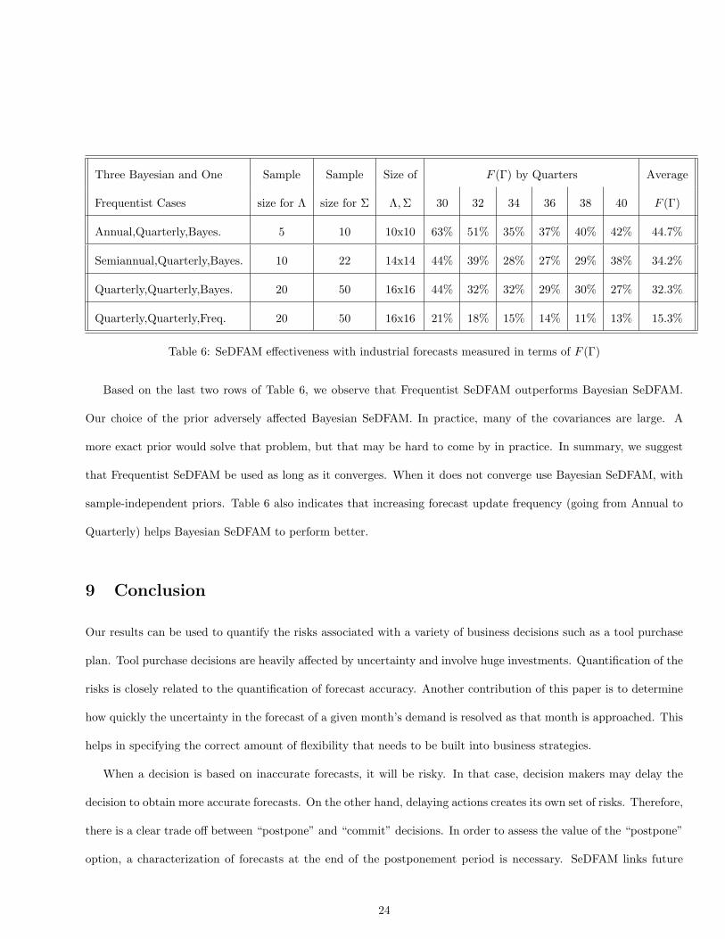
In this section, we will study the effectiveness of SeDFAM with the simulated forecasts. We simulate six product

families with several ramps and study the covariances between two of the families (See Figure 3).

6.1 Simulating a Forecast History

We briefly describe the algorithm used to randomly generate forecast history data dp,tecs,t , for t ≤ now. Family

forecasts dps,t are generated using a given update covariance matrix Λ0. We use equation (7) (replacing ∆ with D

and U with V ) to generate family forecasts starting from forecasts made H = 6 periods in advance.

We use a given perceived ramp age update covariance matrix Σ0 to generate age forecasts, δp,tecs,t , through Equation

(7). Fractional ramp forecasts, fp,tecs,t are obtained from ramp age forecasts via equation (2). The ramp curve we

use is also given and is a symmetric cubic polynomial: R0(δ) = 3δ2 − 2δ3. Sometimes simulated fractional forecasts

14

that are made in the same period are out-of-order, i.e. fp,tecs,t > fp,tec

s,t+1. Since newer technologies replace older ones,

we assume the fp,tecs,t are nondecreasing in t for fixed s. To achieve this, out-of-order fractional forecasts are sorted.

Lastly, product demand forecasts are obtained from the following equation:

dp,tecs,t = {dp

s,t}{fp,tecs,t − fp,tec+

s,t }.

6.2 Two Heuristics: Allocation and Proportion Schemes

We want to compare SeDFAM with other methods. However, to our knowledge there are no forecasting methods that

capture product families and new product technologies, and forecast evolution. Therefore, we have devised two other

forecasting schemes that might be attempted in practice. In the first scheme, family lag-h forecast error variances

(σph)2 = var(Dp

t,t − Dpt−h,t|=t−h) are calculated from the historical family demand. In each period t (t > now),

they are allocated to products by the fractional forecasts made in period now: var((Dp,tect,t − Dp,tec

now,t)|=now) =

(fp,tecnow,t − fp,tec+

now,t )(σpt−now)2. In this Allocation Scheme, product demands are treated as if they were independent.

In the second scheme, called the Proportion Scheme, assume that fractional forecast errors in product demands

depend only on the lag, and are independent of product family and technology. We assume that

ψt−s ∼dp,tec

s,t − dp,tect,t

dp,tecs,t

for t−H ≤ s < t. (15)

We call ψt−s the proportional lag update. Then, in period now,

var((Dp,tect,t −Dp,tec

now,t)|=now) = (dp,tecnow,t)

2var(Ψt−now) (16)

6.3 Base Case

We have structured our numerical study around a base case. In coming up with the base case, we have relied on our

interviews with people in the semiconductor industry (see [1]). We set the available forecast history to 60 months

of data, and the forecast horizon H to six months. We calculated a product family update covariance matrix using

data obtained from a semiconductor manufacturer and based our “true” Λ0 on that. In the base case, on average,

every 8-10 months a new technology is introduced. Technologies stay active almost 24 months. Also note that one

of the product family demands has a linear trend of going up whereas the other is stable (see Figure 3).

15

Our experimental setup is composed of 10 replications. Replications have now dates that are two months apart.

They cover the start, middle and end of the ramp, so that SeDFAM can be evaluated at different phases of the ramp.

Each replication uses 60 months of forecast history.

In applying SeDFAM to the base case, we follow the steps outlined in Table 1. We comment on step 2. It is

possible to estimate a different ramp curve for each technology or for each product family. However, if a ramp curve

is estimated from only 4-5 ramps, it can not be estimated very accurately. Since the forecast history, in practice,

often does not go beyond 4-5 ramps, we suggest that a single R be fit to historical data fp,tecs,t from all families and all

technologies, using 48-60 periods. We fit a piecewise quadratic spline, R, to the fractional forecast data. The spline

has three knots with R(0) = 0, R(L) = 1. It is constrained to have vanishing derivatives at the endpoints {0, L}.

Estimation of Λ is a straightforward application of the Heath-Jackson scheme ([18]). The estimated Λ can be

directly compared to Λ0. This direct comparison is not as meaningful for Σ, because fractional forecasts are sorted.

The quality of the estimates of Λ and Σ are not as important as estimates of the covariances of forecast errors.

We are especially interested in errors in forecasted capacity requirements for specific tools. We focus on a critical

tool, called Ctool, that has processing times (per job) of 1 hour for (A, tec), 1.3 hours for (A, tec+), 0.7 hours for

(B, tec) and 1 hour for (B, tec+). The technology (tec) is introduced on product family A in the 61st month, and

its successor (tec+) in the 68th month. Those technologies (tec and tec+) are introduced on product family B in

the 64th and the 73rd months. The Ctool is not used at all before month 61. Let Cnow,t be the capacity demand

for Ctool in period t as seen from now. Capacity demands for Ctool are obtained by multiplying product demand

forecasts by processing times and summing. Let Cnow = [Cnow+1,now+1, Cnow+2,now+2, ..... , Cnow+H,now+H ].

Starting from a single forecast history covering all periods t, t ≤ now, we randomly generate a sample of 5000

independent future product demands (Dp,tect,t ), t > now. “True” values of all performance measures are derived from

these future product demands.

16

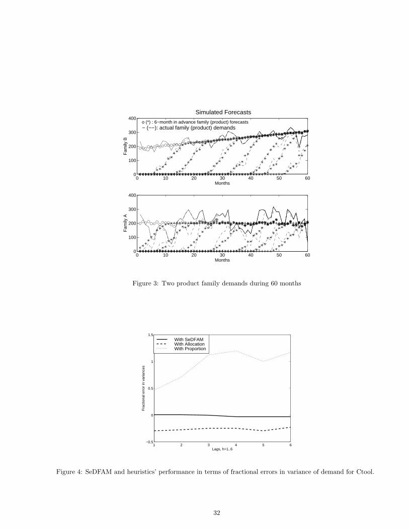
6.4 SeDFAM vs. Allocation and Proportion Heuristics: Estimation and Decision

Making

We apply SeDFAM, and the Allocation and Proportion heuristics to generate estimated variances for the base case.

For each lag, we average the following measure over all replications, and call it the fractional error in variance

Estimated V ariance− True V arianceTrue V ariance

Figure 4 shows the performance of the heuristics against SeDFAM with the Frequentist version of the EM algorithm,

in predicting the demand variance for Ctool.

For the base case, it appears that the Allocation Scheme underestimates the variances: Its estimates are uni-

formly 70% of the true variances. The Allocation Scheme estimates variances for product families correctly, but

it ignores correlations while disaggregating them by technology. In fact demands for succeeding technologies are

negatively correlated, so the disaggregated variances are underestimated. On the other hand, the Proportion Scheme

overestimates variances by 50% to 110%. Large-valued Dp,tecs,t lead to overly large variance estimates (see Equation

(16)).

We now want to see the business implications of inaccurate variance estimation using a simple capacity acquisition

model. We study six type of tools whose installment lead times vary from 2 months to 12 months. All of these tools

have the same processing times as Ctool, described in the previous section. Using variance estimates from SeDFAM,

tools are bought to satisfy the true capacity demand with a probability of 84.1%. Table 3 depicts actual probabilities

of meeting the true capacity demand when capacities are selected according to SeDFAM variance estimates. Similar

computations were done for Allocation and Proportion. For example, for tools with a 2 month lead time (LT=2),

demand is met 76.6% of the time when capacity acquisition is based on Allocation estimates. The target is 84.1%.

The Proportion Scheme overestimates variance, sets capacity levels high, and has infrequent shortages.

Since infrequent shortages are achieved at the expense of buying extra capacity, we also report the ratio of

expected excess tool capacity to expected capacity required (see Table 4). Ratios are converted to percentages for

readability. “True” is the expected excess capacity actually required to meet the demand with a probability of 84.1%.

As expected, Proportion (Allocation) consistently installs too much (not enough) capacity.

17

Method LT=2 LT=4 LT=6 LT=8 LT=10 LT=12 Average error

SeDFAM 83.2 % 82.6 % 83.0 % 83.0 % 83.5 % 83.9 % 0.97%

Allocation 76.6 % 78.1 % 78.5 % 79.1 % 79.7 % 80.0 % 5.52%

Proportion 86.2 % 85.4 % 88.2 % 87.2 % 86.8 % 88.2 % 3.29%

Table 3: Probabilities of meeting capacity demands for tools of lead time=2..12. Target = 84.1 %.

Method LT=2 LT=4 LT=6 LT=8 LT=10 LT=12 Average error

True 22.9 % 34.4 % 33.6 % 35.5 % 33.9 % 33.1 % -

SeDFAM 22.1 % 32.8 % 33.0 % 34.5 % 33.4 % 32.8 % 1.1%

Allocation 18.8 % 29.1 % 28.5 % 30.5 % 29.5 % 29.1 % 5.4%

Proportion 32.8 % 38.5 % 40.7 % 40.7 % 37.8 % 38.5 % 11.4%

Table 4: Ratio of excess capacity to expected capacity required.

Second, we study the effects of inaccurate estimation on revenue prediction. We now suppose that prices are

$1 per unit of (A, tec) , $1.3 for (A, tec+), $0.7 for (B, tec) and $1 for (B, tec+). We assume that all demand

is satisfied and estimate the variance of the total revenue over the next six months. The difference between the

SeDFAM variance estimate and the true variance is scaled by the true variance to obtain fractional errors in 6-month

revenue variances. Fractional errors in variances are also calculated for the heuristics. See Figure 5. In the base

case, demands are positively correlated in time. The Allocation Scheme does not capture these correlations, and

drastically underestimates the 6 month variance. Proportion Scheme estimates are small (large) when the demand

forecasts Dp,tecnow,t are small (large) (see Equation (16)).

6.5 Nonlinearity Bias

In section 4, we discussed nonlinearity bias in fp,tecs,t . There are three interesting quantities to compare. First,

the fractional simulated forecast fp,tecnow,t, from the historical data. Second, the true mean of the fractional demand,

18

E(F p,tect,t |=now). Third, SeDFAM creates R and Σ. We use Σ to estimate the distribution of (∆p,tec

t,t |=now), and use

R to estimate E(R(∆p,tect,t |=now)). All three quantities are converted from fractional demands to demand for Ctool

capacity, resulting in the “Forecast”, the “True Estimate”, and the “SeDFAM Estimate”.

The bias percentage is the difference between either the Forecast or the SeDFAM estimate and the True Estimate,

divided by the Forecast (see Figure 6). This figure depicts nonlinearity bias percentage in 6-month out forecasts for

each of the ten replications whose now dates range from the 60th to the 78th month. In month 78, the tec ramp is

about to end. The nonlinearity bias is too small to have a significant effect on our results.

7 Robustness of SeDFAM

In this section, we test the robustness of SeDFAM against variations in the base case parameters: forecast his-

tory, ramp variability, length of ramp lives, skewedness of ramp curves, covariance structures and forecast horizon.

SeDFAM’s performance is measured in terms of its accuracy in predicting capacity demand covariance matrices.

Step 8 of Table 1 computes variances and covariances of forecasts made in period now. These data are used to

generate an estimate Γ of the covariance matrix of the vector Cnow of capacity demands for Ctool. Let Γ be the true

capacity demand covariance matrix. A performance measure for SeDFAM is F (Γ), defined as

F (Γ) =||Γ− Γ||F||Γ||F

where F denotes the Frobenious norm (||Γ||F = (∑

j

∑

i |Γij |2)1/2). For 10 replications of the Base Case, F (Γ) has

an average value of 8.5%.

In the base case, there are 60 months of forecast history. Naturally, with more historical data, we can estimate Γ

better (see figure 7). Note that estimation errors are within 15% both with history of 60 and 90 months. Thus, by

examining forecast histories beyond 60 months, covariance estimates can not be improved very much. On the other

hand, errors go up to almost 20% when forecast history is halved down to 30 months. As a result, we conclude that

45-60 months of forecast history will deliver satisfactory covariance estimates.

We test the effectiveness of our EM method when the variability in the ramp forecasts changes. For that, we

multiply Σ0 by 2.25 and by 0.25 to obtain two versions that differ from the base case only by ramp variability. We

19

depict the F (Γ) measure (see Table 5) and conclude that the effectiveness of SeDFAM does not depend on ramp

variability.

Ramp life is the length of the S-curve in Figure 1. It is the time from the introduction of a technology until the

obsolescence of the previous technology. Ramp life averages 14 months in the base case. We experiment with average

ramp lives of 10 and 18 months (see Table 5). The improvement is probably due to the increase in the number of

observed data elements per month. The impact on SeDFAM’s accuracy is small.

We investigate the effects of the skewedness of the ramp curve. A symmetric ramp curve satisfies:

R0(t) + R0(L− t) = 1 for 0 < t < L.

The “=” above becomes “>” (“<”) for a left-skewed (right-skewed) ramp curve. Table 5 shows skewedness has a

weak effect on performance.

Both Λ and Σ contain covariances across time and between product families. In this experiment, we first test the

response of our method to higher or lower correlations across time and in product family demands while everything

else is kept constant. We regulate the time-wise covariances by scaling the appropriate submatrices of Λ. High (low)

correlation in the family demand section of Table 5 refers to a situation where month to month demand covariances

inside a product family are approximately increased (decreased) by 100% (50%) and covariances across families

are approximately increased (decreased) by 50% (30%). Second, above experiment is repeated with the ramp age

covariance matrix, Σ. From Table 5, we conclude that relative magnitude of both ramp age and family covariances

have a small effect on SeDFAM performance.

Lastly, Table 5 shows the effect of using forecast horizons H = 6,8,10 and 12 on F (Γ). It is hard to detect a

consistent trend from this table. Thus, we conclude that forecast horizon does not have a clear effect on performance.

8 Industry Example

A semiconductor manufacturer provided us with an industrial data set of annual forecasts with quarterly time

buckets , and with H = 10 quarters. We have 5 years of data from 1994 to 1998. We studied 4 product families and

20

Months 60 62 64 66 68 70 72 74 76 78 Average

Base case 7.3 15.6 6.0 15.4 6.8 6.5 4.5 10.8 5.9 6.1 8.5

Ramp variability

Less 7.1 16.9 9.5 20.4 6.9 7.1 4.6 11.2 6.0 6.1 9.6

More 7.2 16.3 7.6 13.6 4.5 6.5 3.8 11.1 5.9 6.2 8.3

Length of Ramps

L=10 12.1 11.5 10.7 9.4 3.4 13.1 12.3 12.8 8.0 9.2 10.2

L=18 2.4 6.7 3.5 6.0 5.7 12.9 9.7 10.4 8.4 7.0 7.3

Ramp skewedness

Left 9.5 17.5 5.4 19.4 8.5 6.2 6.2 12.2 6.7 6.1 9.8

Right 5.7 23.3 6.7 20.0 8.8 7.2 5.5 12.5 6.9 6.2 10.3

Serial correlation in family demand

Low 8.5 16.3 6.3 13.3 6.1 6.2 4.6 10.8 5.8 6.2 8.4

High 5.9 15.0 7.9 17.0 7.3 6.8 4.4 10.7 6.1 6.1 8.7

Serial correlation in perceived ages

Low 6.2 17.0 7.1 18.8 5.2 7.4 4.8 11.0 6.1 6.1 9.0

High 8.4 16.5 7.1 15.5 5.4 6.5 4.0 10.9 6.0 6.2 8.7

Forecast Horizon, H

H = 8 7.8 11.9 6.7 15.3 17.6 21.3 29.3 30.3 15.1 29.4 18.5

H = 10 12.1 16.4 8.4 12.5 10.4 22.2 8.8 6.6 21.1 11.4 13.0

H = 12 11.5 19.1 18.0 34.1 11.7 19.9 8.2 5.3 18.0 5.5 15.1

Table 5: Robustness of SeDFAM in terms of F (Γ)

21

5 technologies. However, not all technologies are used on all 4 families in all time periods. Figure 8 depicts dps,t and

fp,tecs,t . A single curve in Figure 8 represents either dp

s,t or fp,tecs,t as t ranges from s to s + H.

8.1 Validating SeDFAM Assumptions

The first step in applying SeDFAM is checking the validity of the assumptions. SeDFAM is built on two critical

independence assumptions, (I1) and (I2). (I1) implies the independence of the perceived age update u and the

family update v. Hence, whether a technology is delayed or expedited has no effect on family demands. To improve

significance of the statistical tests, we pool data from all families together. Then, for each forecast lag (6 lags), we

test (for (I1)) the component wise independence of the family and perceived age update vectors that are observed

in the same year. We have 6 tests, each test has on average 20 sample points depending on the pace of ramps.

Assumption (I2) implies the independence of two perceived age updates calculated from two sequential technologies

on the same family. In other words, delaying one technology should not significantly delay the next one. For each

forecast lag (6 lags), we test (for (I2)) the component wise independence of two sequential technologies’ perceived

age updates observed in the same year. There are 6 tests, each with 11-18 sample points.

Independence is tested with a likelihood ratio based parametric test by assuming normality of update vectors

(see pp. 220 Bickel and Doksum [25]). The smallest p-value of the 12 tests (6 for (I1) and 6 for (I2)) is 0.29.

Consequently, (I1) and (I2) assumptions are validated for the industrial forecasts.

Assumption (A1) cannot be tested fully with the given forecast data because, in year r, there is no information

about a forecast made in year s (s > r). Instead, we test the last assertion of (A1). It requires that updates

computed in different periods be uncorrelated (or independent for Normal updates). We tested independence of

family (perceived age) updates with 12 (14) sample points. There is no indication of dependence in family updates

and the test of perceived age update has a p-value of 0.43. Consequently, we conclude that updates are uncorrelated.

Assumption (A2) requires that updates be stationary. In figure 9, we plot perceived age updates versus ramp

ages to see if updates have a pattern or trend. There is no significant trend so assumption (A2) seems reasonable.

Assumption (A3) requires that family and perceived age updates (each of length 2) have mean zero. In this test,

sample size is 16 for family updates and between 19 and 21 for perceived age updates. Our tests find only two-year-

22

out family updates unbiased. One-year-out family updates have negative bias. In other words, family forecasts are

optimistic initially and they are decreased to realistic levels one year before the demand is observed. Our tests find

perceived age forecasts positively biased, i.e., initially ramp schedules are overly pessimistic. In summary, forecast

data indicates biased family updates and perceived age updates. See Appendix C for discussion on how to adapt

SeDFAM for these “Lag Biases” in updates.

8.2 Effectiveness of SeDFAM for Industrial Forecasts

Having justified SeDFAM assumptions, we use the industrial data to test how SeDFAM responds to lower up-

date frequencies. We consider three cases with the following forecast update frequencies and time buckets: (An-

nual,Quarterly), (Semiannual,Quarterly) and (Quarterly,Quarterly). We estimate Λ0 and Σ0 from the industrial

data for families A and B of Figure 8 and compute F (Γ) as in Table 5. In all cases, we run SeDFAM with H = 8

quarters and 20 quarters of forecast history. In the (Annual, Quarterly) case, in quarter t we see demand forecasts

for quarters t, ..., t + 8. The most recent previous forecast was made in t − 4, for quarters t − 4, ..., t + 4. Those

forecasts have 5 overlapping quarters t, ..., t + 4 and two families, so Λ and Σ are 10 x 10 matrices.

We summarize the performance of SeDFAM in Table 6. The second and third columns contain the approximate

number of observations used in estimating Λ,Σ respectively. As forecast update frequency increases (from once

to four times in a year), the size of the covariance matrices and the number of observations both grow. In the

(Annual,Quarterly) and (Semiannual,Quarterly) cases, sample sizes are small with respect to the size of Σ so the

Frequentist version of the EM algorithm diverges without yielding a Σ. To circumvent this, we use the Bayesian

version of the EM algorithm in step 7 of SeDFAM (first three rows of Table 6). For comparison, the last row shows

the performance of the Frequentist version of SeDFAM.

For Bayesian estimation we use the Inverted-Wishart prior (see pp. 150 of Schafer [24]). With this prior, we

set the expected value of the updates equal to zero. Interview data ( [1]) indicates that practitioners have a fairly

good grasp of variances, but little understanding of covariances. Thus we selected a diagonal matrix for the expected

value of Σ. All diagonal elements for a given family are equal, meaning that in the prior, the variance of the forecast

errors (δt,t − δt−h,t) is a linearly increasing function of the forecast lag h.

23

Three Bayesian and One Sample Sample Size of F (Γ) by Quarters Average

Frequentist Cases size for Λ size for Σ Λ,Σ 30 32 34 36 38 40 F (Γ)

Annual,Quarterly,Bayes. 5 10 10x10 63% 51% 35% 37% 40% 42% 44.7%

Semiannual,Quarterly,Bayes. 10 22 14x14 44% 39% 28% 27% 29% 38% 34.2%

Quarterly,Quarterly,Bayes. 20 50 16x16 44% 32% 32% 29% 30% 27% 32.3%

Quarterly,Quarterly,Freq. 20 50 16x16 21% 18% 15% 14% 11% 13% 15.3%

Table 6: SeDFAM effectiveness with industrial forecasts measured in terms of F (Γ)

Based on the last two rows of Table 6, we observe that Frequentist SeDFAM outperforms Bayesian SeDFAM.

Our choice of the prior adversely affected Bayesian SeDFAM. In practice, many of the covariances are large. A

more exact prior would solve that problem, but that may be hard to come by in practice. In summary, we suggest

that Frequentist SeDFAM be used as long as it converges. When it does not converge use Bayesian SeDFAM, with

sample-independent priors. Table 6 also indicates that increasing forecast update frequency (going from Annual to

Quarterly) helps Bayesian SeDFAM to perform better.

9 Conclusion

Our results can be used to quantify the risks associated with a variety of business decisions such as a tool purchase

plan. Tool purchase decisions are heavily affected by uncertainty and involve huge investments. Quantification of the

risks is closely related to the quantification of forecast accuracy. Another contribution of this paper is to determine

how quickly the uncertainty in the forecast of a given month’s demand is resolved as that month is approached. This

helps in specifying the correct amount of flexibility that needs to be built into business strategies.

When a decision is based on inaccurate forecasts, it will be risky. In that case, decision makers may delay the

decision to obtain more accurate forecasts. On the other hand, delaying actions creates its own set of risks. Therefore,

there is a clear trade off between “postpone” and “commit” decisions. In order to assess the value of the “postpone”

option, a characterization of forecasts at the end of the postponement period is necessary. SeDFAM links future

24

forecasts to current forecasts by studying forecast evolution. It captures improvement in forecasts as time goes by.

Consequently, SeDFAM is a natural tool to use in postponement vs. commitment trade offs.

Measuring forecast accuracy methodologically (with the covariance matrices) helps monitor forecast quality. By

monitoring forecast quality, one can signal when forecasts deteriorate, or when a major shock affects the forecasts

(i.e., the Taiwan earthquake). With SeDFAM, one can even identify whether family demand forecasting or ramp

age forecasting is causing the deterioration. We have also provided algorithms for simulating demands and forecasts

realistically recognizing dependences among product demands. Such simulations often constitute the primary input

for simulation (scenario) based decision making techniques.

By studying the performance of SeDFAM under parametrically varied situations, we have empirically shown that

SeDFAM is robust against ramp variability, ramp skewedness and the relative magnitude of time-wise or family-wise

covariances. SeDFAM is also robust against the length of ramp lives and forecast horizons. On the other hand,

length of forecast history affects performance, especially when forecast history is shorter than 45 months. In its

current form, for SeDFAM to work with 5 years of historical data, forecasts should be updated quarterly. If forecast

updates are less frequent, a Bayesian version of SeDFAM would be more appropriate.

When our assumptions hold, SeDFAM performs very well. Those assumptions are based on our interviews with

semiconductor manufacturers and have been validated using an industrial data set. It is possible to relax some of

our assumptions at the expense of added complexity or to simplify our approach in specific situations. However, as

it is now, we believe that SeDFAM strikes a good balance between complexity and utility.

25

Appendix A: Commonly Used Notation

• p: A generic product family. tec: A generic manufacturing technology. (p, tec): A generic product.

• r, s, t, w: Time periods.

• dps,t: Demand forecast for product family p, from s for t. Dp

s,t: Random variable for dps,t before period s.

• dp,tecs,t : Demand forecast for product (p, tec), from s for t.

• fp,tecs,t : Forecast for fraction of products in family p, which are manufactured with technology tec or newer

technologies, from s for t.

• δp,tecs,t : Forecast for perceived (p, tec)-ramp age, from s for t. ∆p,tec

s,t : Random variable for δp,tecs,t before period s.

• H: Forecast horizon. L: Ramp length.

• =r: Information available in period r.

• vps,t: Product family p demand forecast update observed in period s.

• up,tecs,t : Perceived (p, tec)-ramp age forecast update observed in period s.

• vs: Product family demand forecast update vector, observed in period s. Vs: Random vector for vs before

period s.

• utecs : Perceived age forecast update vector, observed in period s. U tec

s : Random vector for utecs before period s.

• Cnow,t: Random variable for the capacity demand of a critical tool in period t, as seen from now (now < t).

• Cnow = [Cnow+1,now+1, Cnow+2,now+2, ..... , Cnow+H,now+H ].

• Λ: Covariance matrix for Vs. Σ: Covariance matrix for U tecs . Γ: Covariance matrix for Cnow.

• F (Γ): Frobenious norm of matrix Γ.

26

Appendix B: Demands with Trend and Seasonality

Assume that our family demands, dpt,t, have trend and/or seasonality. We seek a transformed series dp

t,t that has

trend and seasonality in its mean µt, but for which dpt,t−µt is a stationary time series. We assume that the forecasts

inherit this property, i.e., dpt−h,t − µt is stationary for all h, 0 ≤ h ≤ H. Under this assumption the µt terms cancel

out when computing updates and can be ignored, i.e.,

vpt−h,t = dp

t−h,t − dpt−h−1,t

has mean zero and stationary variance as required by Assumption (A2).

The literature has two approaches for obtaining dpt,t. The standard approach is to stabilize variance with a

transformation g, i.e., dpt,t = g(dp

t,t). The most popular transformations are g(d) = log d and g(d) = (dλ − 1)/λ,

λ 6= 0 (see Brockwell and Davis [22], and Box and Cox [26]).

The second approach assumes dpt,t = m(t, β) + s(t, θ)wt, where wt is stationary with mean 0 and variance 1.

If there are L time periods in a season then β = (a, b, s1, ..., sL) and m(t, β) = a + b t + S(t mod L)+1 capturing

the combined effects of trend and seasonality. θ and s(t, θ) are similar. The vectors β and θ are parameters to be

estimated. After estimating θ we can set dpt,t = dp

t,t/s(t, θ).

A generalized least squares algorithm can be used to estimate β and θ. We recommend steps 1-5 of algorithm

on pp. 69-70 of Carroll and Ruppert [27]. Step 2 of that algorithm can be based on section 3.3.1. of [27], with

yt = dpt,t, f(xt, β) = m(t, β), g(µ1(β), zt, θ) = s(t, θ), and σ = 1.

Appendix C: Forecasts with Lag Bias

Let us focus on a product p, tec and drop p, tec indices. Suppose that perceived age forecast are lag biased, i.e.

as opposed to Equation (8) δs,t = E(∆t,t|=s) + lb(t− s), where lb(t− s) denotes the deterministic bias as a function

of the lag t− s. By equation (5), us,t = δs,t − δs−1,t. Now because of the lag bias,

E(Us,t) = E(Us,t|=s−1) = lb(t− s)− lb(t− s + 1) 6= 0.

Thus, in step 6 of SeDFAM we need to estimate the expected value of perceived age updates in addition to covariances.

Note that shifting a random variable does not affect its variability, so Us,t and Us,t − lb(t − s) + lb(t − s + 1) have

27

the same variances. Then, covariance matrix of updates can be estimated with the techniques used before, except

that in covariance estimations multiplications of deviations from the mean are divided by sample size minus one

(as opposed to sample size). Thus, we can accommodate lag bias by making moderate changes to SeDFAM. Above

argument also applies to lag-biased family forecasts dps,t.

Acknowledgment : This work was supported by a grant from Semiconductor Research Cooperation under

the task “Modeling Random Processes”, and by the National Science Foundation under the grant DMI-9713549.

The authors would like to thank to Joseph L. Schafer for allowing us to use his EM software, and representatives

of several semiconductor manufacturers for the information and data they made available to us. The authors also

thank to referees for valuable comments that improved the paper’s exposition.

References

[1] Cakanyıldırım, M. and R.O. Roundy. (1999). Demand forecasting and capacity planning in the semiconductor

industry. Technical Paper no: 1229, SORIE, Cornell University, NY.

[2] Meixell, M.J. and S.D. Wu. (2001). Scenario analysis of demands in a technology market using leading indicators.

IEEE Transactions on Semiconductor Manufacturing, Vol.14, No.1: 1-11.

[3] Hamilton, J. D. (1994). Time Series Analysis. Princeton University Press, New Jersey.

[4] Mahajan, V. and Y. Wind (1988). New product forecasting models. International Journal of Forecasting No.4:

341–358.

[5] Murray, G and Silver, E. (1966). A Bayesian analysis of the style goods inventory problem. Management Science

Vol.12, No.11: 785–797.

[6] Chang, S.H. and Fyffe, D.E. (1971) Estimation of forecast errors for seasonal-style-goods sales Management

Science Vol.18, No.3: 89–96.

[7] Bass, F. (1969). A New product growth model for consumer durables. Management Science Vol.15, No.5: 215–227.

28

[8] Norton, J. and F. Bass (1987). A Diffusion theory model of adoption and substitution for successive generations

of high technology products. Management Science Vol.33, No.9: 1069–1086.

[9] Kurawarwala, A.A. and Matsuo, H. (1996). Forecasting and inventory management of short life cycle products.

Operations Research Vol.44, No.1: 131–150.

[10] Guerrero, V.M. and Elizondo, J.A. (1997). Forecasting a cumulative variable using its partially accumulated

data. Management Science Vol.43, No.6: 879-889.

[11] Kekre, S., Morton, T. and Smunt, T. (1990). Forecasting using partially known demands. International Journal

of Forecasting No.6: 115–125.

[12] Bodily, S.E. and J.R. Freeland (1988). A simulation of techniques for forecasting shipments using firm orders-

to-date. Journal of Operational Research Society Vol.39. No.9: 833–846.

[13] Azoury, K. (1985). Bayes solution to dynamic inventory models under unknown demand distribution. Manage-

ment Science Vol.31, No.9: 1150–1160.

[14] Bunn, D.W. and A.A. Salo. (1993). Forecasting with scenarios. European Journal of Operational Research No.68:

291–303.

[15] Angelus, A., Porteus, E.L. and Wood, S.C. (1997) Optimal sizing and timing of capacity expansions with impli-

cations for modular semiconductor wafer fabs. Research Paper No.1479. Graduate School of Business, Stanford

University.

[16] Hausman, W. (1969). Sequential decision problems: A model to exploit existing forecasters. Management Science

Vol.16, No.2: B-93–B-111.

[17] Graves, S.C., H.C. Meal, S. Dasu and Y. Qui (1986). Two stage production planning in a dynamic environment.

In Multi-Stage Production Planning and Inventory Control. S. Axsater, C. Schneeweiss and E. Silver, (eds.),

Lecture notes in economics and Mathematical systems, Springer-Verlag, Berlin, 266: 9-43.

29

[18] Heath, D. and Jackson, P. (1994). Modeling the evolution of demand forecasts with application to safety stock

analysis in production/distribution systems. IIE Transactions Vol.26, No.2: 17–30.

[19] Gullu, R. (1996). On the value of information in dynamic production inventory problems under forecast evolu-

tion. Naval Research Logistics Vol.43: 289–303.

[20] Toktay, L.B. (1998). Analysis of a production-inventory system under a stationary demand process and forecast

updates. Unpublished Ph.D. dissertation, Operations Research Center, MIT, Cambridge, MA.

[21] Graves, S.C., D.B. Kletter and W.B. Hetzel (1998). A dynamic model for requirements planning with application

to supply chain optimization. Operations Research Vol.46, Supp. No.3: S35-S49.

[22] Brockwell, P. and R.A. Davis. (1987). Time Series: Theory and Methods. Springer-Verlag New York Inc.

[23] Anderson, T.W. (1984). An introduction to multivariate statistical analysis. John Wiley & Sons, Inc. New York.

[24] Schafer, J.L. (1996). Analysis of Incomplete Multivariate Data. Chapman and Hall, London.

[25] Bickel, P.J. and K.A. Doksum (1977). Mathematical Statistics. Simon & Schuster Company, New Jersey.

[26] Box, G.E.P. and D.R. Cox (1964). An analysis of transformations. Journal of the Royal Statistical Society Series

B Vol.26, No.2: 211-243.

[27] Carroll, R.J. and D. Ruppert. (1988). Transformation and Weighting in Regression. Chapman and Hall, New

York.

30

CM

OS

10C

MO

S 12

CM

OS

8

Tim

e

Prod

uct D

eman

dM

emor

y D

eman

d

Mem

ory

Dem

and

S-cu

rve

for

CM

OS

8;S-

curv

e fo

r C

MO

S 10

;S-

curv

e fo

r C

MO

S 12

;

Figure 1: Technology migration in a product family

Perceived Agesδp,tecr,t = ∆p,tec

r,t |=r.

?

Perceived Age UpdatesU tec

s = (Up,tecs,t ) ∼ N(0,Σ).

?

Perceived Age Forecasts ∆p,tecs,t = ∆p,tec

s−1,t + Up,tecs,t , see (3).

?Fractional Demand Forecasts F p,tec

s,t = R(∆p,tecs,t ), see (2).

?

Family Demandsdp

r,t = Dpr,t|=r.

?

Family Demand UpdatesVs = (V p

s,t) ∼ N(0, Λ).

?

Family Demand Forecasts Dps,t = Dp

s−1,t + V ps,t, see (3).

?Product Demand Forecast Dp,tec

s,t = Dps,t(F

p,tecs,t − F p,tec+

s,t ), see (1).

Figure 2: Hierarchical probability model for forecasts.

31

0 10 20 30 40 50 600

100

200

300

400

Months

Fam

ily A

0 10 20 30 40 50 600

100

200

300

400

Months

Fam

ily B

Simulated Forecasts

o (*) : 6−month in advance family (product) forecasts − (−−): actual family (product) demands

Figure 3: Two product family demands during 60 months

1 2 3 4 5 6−0.5

0

0.5

1

1.5

Fra

ctio

nal e

rror

in v

aria

nces

Lags, h=1..6

With SeDFAM With AllocationWith Proportion

Figure 4: SeDFAM and heuristics’ performance in terms of fractional errors in variance of demand for Ctool.

32

60 62 64 66 68 70 72 74 76 78−0.8

−0.6

−0.4

−0.2

0

0.2

0.4

0.6

Fra

ctio

nal e

rror

in 6

−m

onth

rev

enue

var

ianc

e

Starting Months for Replications

With SeDFAM With AllocationWith Proportion

Figure 5: Fractional errors in 6 month revenue variance estimates.

60 62 64 66 68 70 72 74 76 78−1.5

−1

−0.5

0

0.5

1

1.5

2

2.5

Bia

s pe

rcen

tage

Starting Months for Replications

Forecast SeDFAM Estimate

Figure 6: Nonlinearity bias in 6 months in advance forecasts.

33

55 60 65 70 750

0.05

0.1

0.15

0.2

0.25

0.3

0.35

0.4

F(Γ

)

Starting Months for Replications

90 month aver. 60 month aver.

45 month aver.

30 month aver.

x, o, +, * : individual runswith 90, 60, 45, 30 months of forecast history

Figure 7: Effectiveness of SeDFAM estimates as forecast history varies.

5 10 15 20 250

1

2

3

Fam

ily A

Family Forecasts

5 10 15 20 250

0.5

1

Fam

ily A

Fractional Ramp Forecasts

5 10 15 20 250

1

2

3

Fam

ily B

5 10 15 20 250

0.5

1

Fam

ily B

5 10 15 20 250

1

2

3

Fam

ily C

5 10 15 20 250

0.5

1

Fam

ily C

5 10 15 20 250

1

2

3

Quarters

Fam

ily D

5 10 15 20 250

0.5

1

Quarters

Fam

ily D

Figure 8: Family forecasts, dps,t and fractional ramp forecasts, fp,tec

s,t . Both are for four product families A, B, C and

D. Each style of curve in the fractional ramp forecasts represents a different technology.

34

0 5 10 15 20 25−15

−10

−5

0

5

10

15

Ramp age

Per

ceiv

ed a

ge u

pdat

e

Figure 9: Perceived age updates vs. ramp ages

35