Embed Size (px)
Citation preview

SEDIMENT CHARACTERISTICS AND BIOAVAILABILITY
OF SORBED NEUTRAL ORGANIC COMPOUNDS
THESIS
Presented to the Graduate Council of the
University of North Texas in Partial
Fulfillment of the Requirements
For the Degree of
MASTER OF SCIENCE
By
Burton C. Suedel, B.S.
Denton, Texas
December, 1989
1-7A/
/Vo.

Suedel, Burton C., Sediment Characteristics and
Bioavailability of Sorbed Neutral Organic Compounds. Master
of Science (Biology), December, 1989, 144 pp., 24 Tables, 14
Figures, References, 53 Titles.
Several sediment characteristics were analyzed to
determine their suitability for use as potential
normalization factors for the bioavailability of neutral
organic compounds sorbed to sediments. Percent organic
carbon, cation exchange capacity and particle surface area
were measured sediment characteristics that varied
sufficiently to encompass the range in observed sediment
toxicity. Laboratory sediment toxicity test data using
fluoranthene suggest that there is no biologically
significant correlation between sediment toxicity and
sediment characteristics (organic carbon, cation exchange
capacity, particle size distribution, particle surface
area). Fluoranthene amended sediments with similar organic
carbon contents do not yield similar toxicities due to
sorbed fluoranthene and thus do not support the organic
carbon normalization approach for evaluating sediment
quality or for sediment criteria development.
I'll :::: 11 WVW '- - -; ---- ON@" 1101111111 11111111,100181 1 IN ommommil

TABLE OF CONTENTS
PageLIST OF TABLES . . . . . . . . . . . . . . . . . . . . . iv
LIST OF FIGURES . . . . . . . . . . . . . . . . . . . . vi
Chapter
1. INTRODUCTION . . . . . . . . . . . . . . . . . 1
Organic Carbon Normalization ApproachSediment Characteristics as NormalizationFactors
Physical Properties of FluorantheneSources of FluorantheneEffects of Fluoranthene on Aquatic Organisms
Acute ToxicityChronic Toxicity
Fluoranthene PartitioningAcute Versus Chronic Effects of ChemicalsResearch ObjectivesHypotheses
2. MATERIALS AND METHODS.. . . . . . . . . . . . . 15
Phase I. Sediment Collection andCharacterization
Phase II. Toxicity TestingTest OrganismsTest SedimentsToxicity Test SedimentsTest Organism Culture Procedures
Daphnia magnaHyalella aztecaChironomus tentans
Testing ProceduresTest WaterScreening TestsRange - Finding TestsDefinitive Tests
Analytical ProceduresWaterSedimentInterstitial Water
Statistical Procedures
ii

TABLE OF CONTENTS CONTINUED
Chapter Page
3. RESULTS........................... .......29
Sediment CharacteristicsBehavioral and Other Subjective ObservationsToxicity Testing
Chironomus TestsHyalella TestsDaphiia Tests
4. DISCUSSION..........................0......63
Sediment CharacterizationToxicity TestingConclusions
APPENDIX A
APPENDIX B
APPENDIX C
APPENDIX D
APPENDIX E
APPENDIX F
REFERENCES
- - - - 1- So -......... ...........76Sediment Collection Summary Sheet
- - - (D-0-0-0.0 0.41 . . ........... . ..... 78Sediment Analysis Procedures
- - - 4- - . - . . . 0- 0 0. 0. 0. 0. . . . . . . 102Organism Culture Procedures
- - -s - - - - . - .10 . 0. 0. 4. . . . . . . . 112Organism Testing Procedures
- - - - -1- -1- - 0 - ...- .......... . 126Sediment Spiking Procedure Using Fluoranthene
- - - - 4- - - - - 0- 0- 0. 0 0. 0. 4. 0.0.d. . . 1. 128Spectrophotometric Analysis of Fluoranthene
- - - - go - - - 0- 411 -0 -0 41 . . .9 .0 .0 .0 .0 . 139
iii
mmwm*N4vm wwouwam ifamp -

LIST OF TABLES
Table Page
I. Sediment Storage and Handling for EachAnalysis . . . . . . . . . . . . . . . . . . . . 17
II. Sediment Parameters and CorrespondingAnalysis..-.................... .. 18
III. Sediment Characteristics and CorrespondingValues for Sediments Used During ToxicityTesting. .-.....-... . . . . . . . . . . . 21
IV. Water Research Field Station (WRFS) Pond WaterCharacteristics.. ... . . . . . . . . . . . . 23
V. Water Analysis Methods and References . . . . . 25
VI. Range, Mean, Standard Deviation and Number ofReplicates for Each Parameter of FreshwaterSediment Samples....-.. . . . . . . . . . . . 30
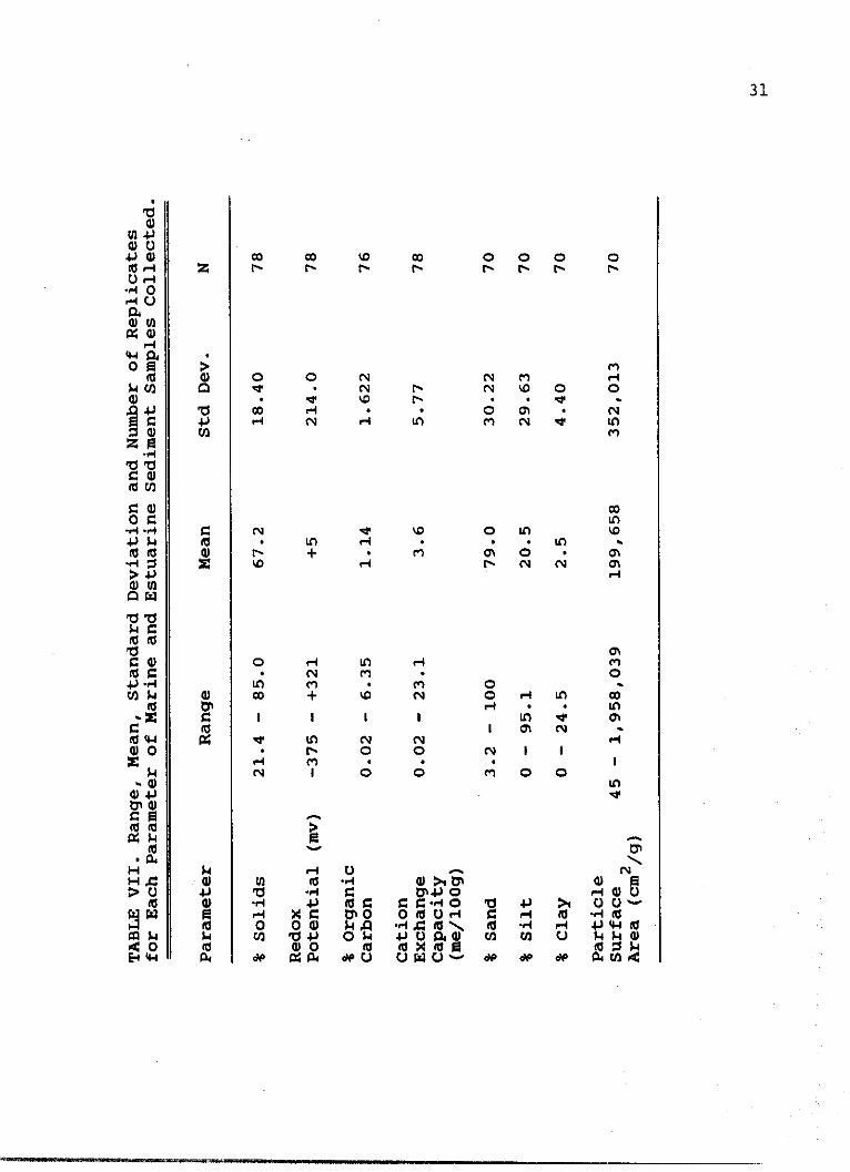
VII. Range, Mean, Standard Deviation and Number ofReplicates for Each Parameter of Marine andEstuarine Sediment Samples . . . . . . . . . . . 31
VIII. Designated Number, Name, and Number of Sites forEach Province Identified During This Study . . . 33
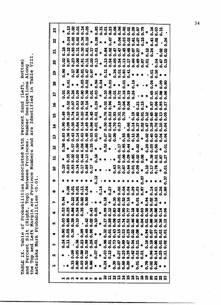
IX. Table of Probabilities Associated With PercentSand (Left, Bottom) and Percent Silt (Right, Top)Between Provinces . . .... .. . . . . . . . . . 34
X. Table of Probabilities Associated With PercentClay (Left, Bottom) and Surface Area (Right, Top)Between Provinces.. . . . . . . . . . . . . . 35
XI. Table of Probabilities Associated With PercentOrganic Carbon (Left, Bottom) and Cation ExchangeCapacity (Right, Top) Between Provinces . . . . 36
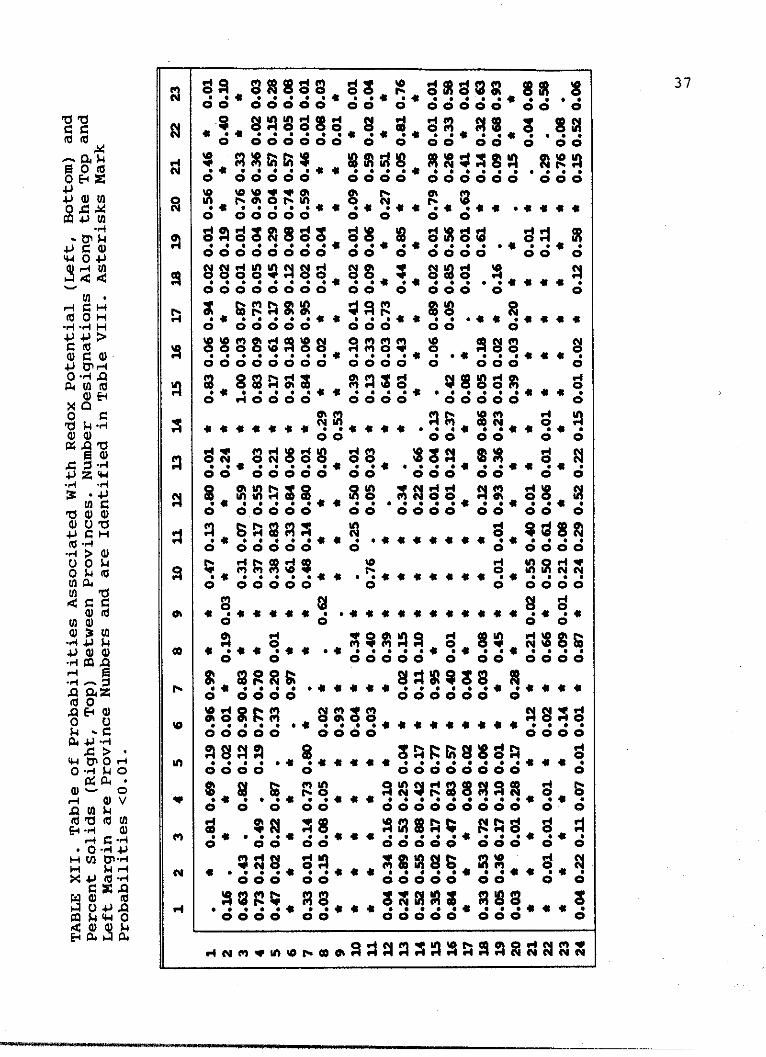
XII. Table of Probabilities Associated With RedoxPotential (Left, Bottom) and Percent Solids(Right, Top) Between Provinces . . . . . . . . . 37
XIII. Pearson Correlation Coefficients and Number ofReplicates (N) for Each Coefficient Listed . . . 39
iv
.11 ;,--, . , , ;;- il. -, -. . ",-vk9a

LIST OF TABLES CONTINUED
Table Page
XIV. Comparison of EC50 Values Between 10 Day Aqueousand Whole Sediment Tests for Each OrganismStudied......................................40
XV. Effects of Fluoranthene on C. tentans Using WaterResearch Field Station Sediment ............. 43
XVI. Effects of Fluoranthene on C. tentans Using LakeFork Reservoir Sediment ...... . . . . . ..... 44
XVII. Effects of Fluoranthene on C. tentans UsingTrinity River Sediment.o...................45
XVIII. Effects of Fluoranthene on H. azteca Using WaterResearch Field Station Sediment .......... 46
XIX. Effects of Fluoranthene on H. azteca Using LakeFork Reservior Sediment ............ ......... 47
XX. Effects of Fluoranthene on H. azteca Using TrinityRiver Sediment..............................48
XXI. Effects of Fluoranthene on D. magna Using WaterResearch Field Station Sediment..............49
XXII. Effects of Fluoranthene on D. magna Using LakeFork Reservior Sediment..................50
XXIII. Effects of Fluoranthene on _. magna Using TrinityRiver Sediment.............. ...4.0 . . ...... 51
XXIV. Comparison of Means of Freshwater and MarineSediments Collected from Various Sources SampledThroughout the United States ..0............... 64
V
w- i WAlWAMMRWMJJW , - -, - - ,
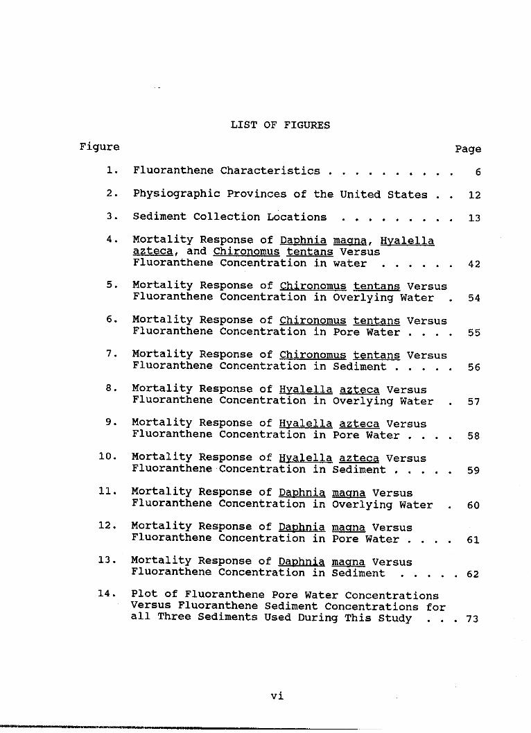
LIST OF FIGURES
Figure Page
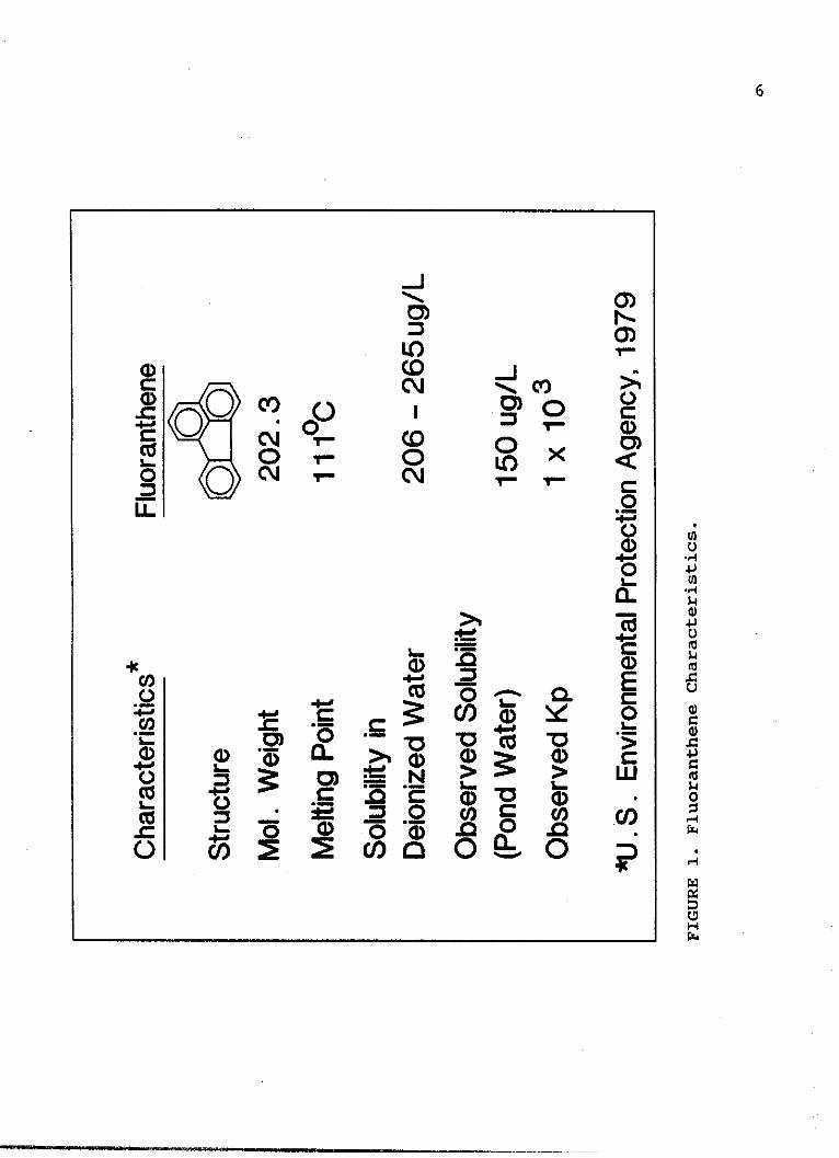
1. Fluoranthene Characteristics .e..........6
2. Physiographic Provinces of the United States 12
3. Sediment Collection Locations................13
4. Mortality Response of Daphnia magna, Hyalellaazteca, and Chironomus tentans VersusFluoranthene Concentration in water. . ..... 42
5. Mortality Response of Chironomus tentans VersusFluoranthene Concentration in Overlying Water . 54
6. Mortality Response of Chironomus tentans VersusFluoranthene Concentration in Pore Water . . . . 55
7. Mortality Response of Chironomus tentans VersusFluoranthene Concentration in Sediment ...... 56
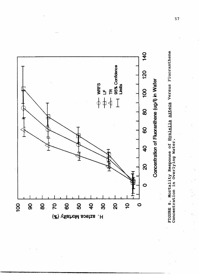
8. Mortality Response of Hyalella azteca VersusFluoranthene Concentration in Overlying Water . 57
9. Mortality Response of Hyalella azteca VersusFluoranthene Concentration in Pore Water . . . . 58
10. Mortality Response of Hyalella azteca VersusFluoranthene Concentration in Sediment . . . . . 59
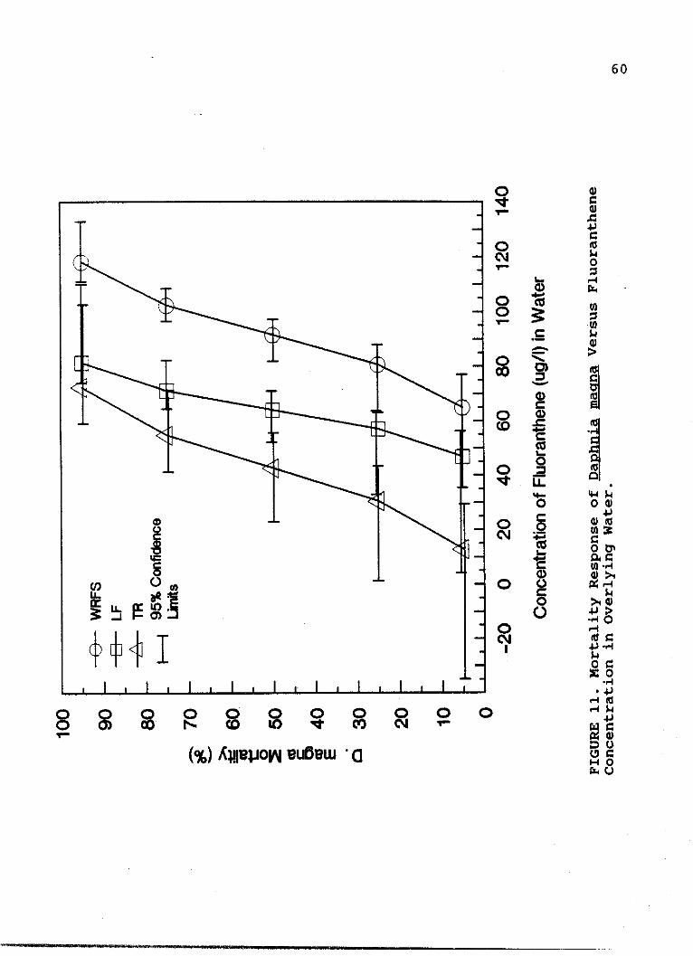
11. Mortality Response of Daphnia magna VersusFluoranthene Concentration in Overlying Water . 60
12. Mortality Response of Daphnia magna VersusFluoranthene Concentration in Pore Water . . . . 61
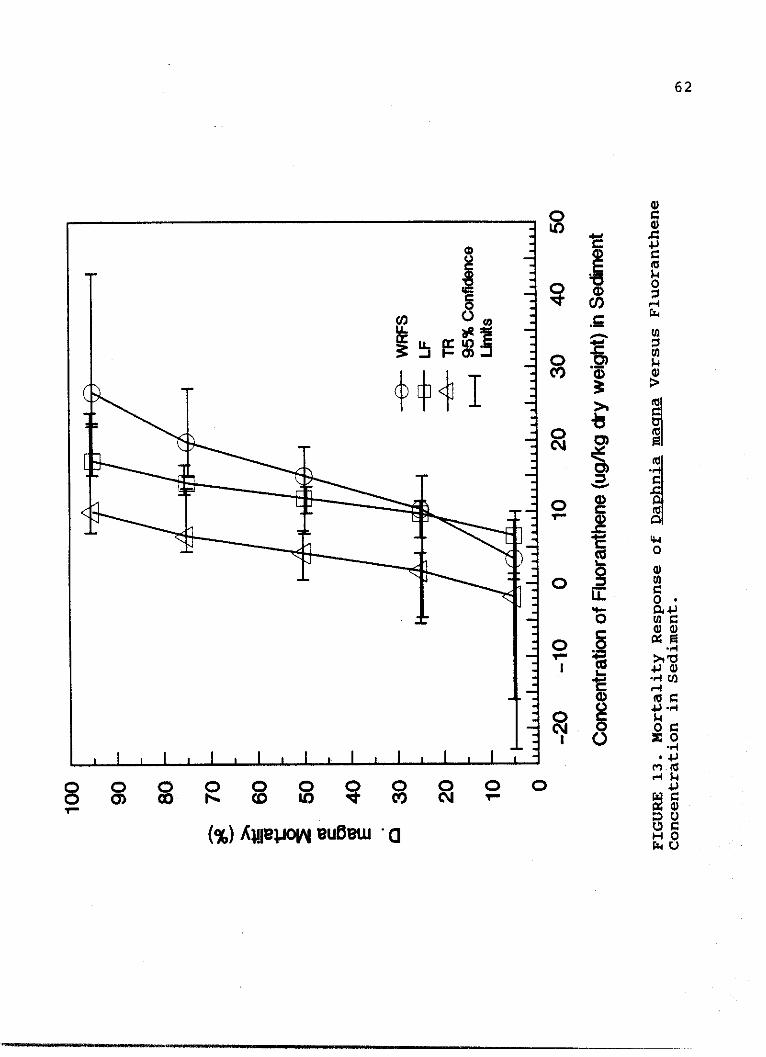
13. Mortality Response of Daphnia magna VersusFluoranthene Concentration in Sediment ........ 62
14. Plot of Fluoranthene Pore Water ConcentrationsVersus Fluoranthene Sediment Concentrations forall Three Sediments Used During This Study . . . 73
vi

CHAPTER I
INTRODUCTION
Recently, concern has been expressed about the ability
of the U.S. Environmental Protection Agency's (EPA) Water
Quality Criteria (WQC) to sufficiently ensure protection of
aquatic life within the provisions of the Clean Water Act
(Battelle, 1985). Degradation of aquatic systems has been
noted in some areas where WQC have not been exceeded in
recent history (JRB Associates, 1984; Lyman, 1987). In
response to these concerns, EPA may develop numerical
criteria for chemicals in sediments [(Sediment Quality
Criteria (SQC)] and apply them to geographic locations
containing sediments with significant amounts of potentially
toxic materials.
The rationale for this approach is that concentrations
of potentially toxic materials in sediments that are greater
than proposed SQC would suggest that these sediments are
potentially toxic or hazardous. Clearly, this could have a
significant impact on industry. If SQC are underprotective,
then many benthic communities could be lost. However, if SQC
are too protective, then this could inhibit chemical
development and possibly deprive society of potentially
beneficial chemicals. First, bottom or consolidated
1
*Awl* 6V '

2
sediments serve as sinks for many potentially toxic
materials (Lyman, 1987; Pavlou, 1987), and long-term
effluent discharges could lead to toxic contaminant
concentrations in the sediments of receiving freshwater,
marine or estuarine systems. In addition, relatively large
numbers of organisms live in and around bottom sediments.
Therefore, sediment contaminant concentrations could be as
important as water concentrations in establishing National
Pollution Discharge Elimination System (NPDES) permit limits
and accomplishing the goals of the Clean Water Act. Several
approaches have been proposed for development of SQC.
Organic Carbon Normalization Approach
Organic carbon (OC) content of sediments has been
proposed as a normalizing factor for bioavailability of
neutral organic compounds sorbed to sediments (Shea, 1988).
If a compound is bioavailable, then it should elicit some
response from an organism. The organism's response is a
function of exposure concentration and duration of exposure.
The organic carbon normalization approach implies that the
bioavailable fraction of a toxic material in a sediment is
governed or moderated by the total organic carbon content of
that sediment. According to the theory, as the OC content of
the sediment increases, the toxicity of the contaminated
sediment concomitantly decreases. Use of this normalizing

3
factor for SQC involves using the concentration of the toxic
material in sediment as the numerator and using the OC
content (%) as the denominator. The resultant number is
hypothesized to be a closer approximation of the
bioavailable concentration of the toxic material:
TOXICANTCONCENTRATIONIN SEDIMENT----------- = ESTIMATED BIOAVAILABLE
SEDIMENT OC(%) CONCENTRATION IN SEDIMENT
There are at least two concerns with the organic carbon
normalization approach for development of SQC. First, there
is no established relationship between sediment toxicity and
bulk chemistry or quantity of toxic materials in sediments
(Battelle, 1985). The mere presence of potentially toxic
materials in sediments does not guarantee that these
sediments are toxic to aquatic life. Secondly, using OC as a
normalizing factor for SQC may or may not be appropriate. An
implicit assumption is that OC content in sediments varies
at least two orders of magnitude because observed toxicity
ranges from zero to 100 percent. Adams (1987) has shown that
OC content of sediments collected across the U.S. has a mean
of 2.0% and that 96% of the values were within two orders of
magnitude (0.1 to 10%). Mathematically, if the OC content of
sediment is less than 1%, then the bioavailable fraction of
toxic materials would theoretically be greater than the

4
measured sediment concentration. It appears that organic
carbon might not vary sufficiently in aquatic sediments for
use as a normalizing factor as intended (Rodgers et al.
1987). A key to this dilemma is that sediments with similar
OC contents and concentrations of toxic materials may vary
widely in observed toxicity (from 0 - 100% mortality). This
is addressed below.
Sediment Characteristics as Potential Normalization Factors
Organic carbon content of sediments is the most
recognized parameter suggested to control bioavailability of
neutral organic compounds (Adams, 1987). However, other
sediment characteristics have not received much attention as
potential normalization factors. Kimerle (1987) stressed the
importance of determining the effects of clay particles and
other important factors on the availability of chemicals in
sediments. Lyman (1987) lists particle size as a possible
covariate with organic carbon in determining chemical
partitioning in sediments. Malueg et al. (1987) raised the
question whether or not physical characteristics of
sediments such as grain size are important in sediment
contaminant concentrations. For example, in contaminated New
York Bight sediments, contaminant concentrations were
strongly related to grain size and organic carbon content.
Cation exchange capacity and organic carbon have also been
mom"" " n , , - 11

5
suggested to affect bioavailability of polar or ionizable
organic compounds (Fava et al. 1987). Organic chemicals of
petroleum origin that are relatively water insoluble should
be good models to test hypotheses regarding regulation of
toxicant bioavailability by sediment characteristics.
Fluoranthene is an example of an organic chemical with a
propensity to sorb to sediments that may be toxic at a
fraction of its aqueous solubility.
Physical Properties of Fluoranthene
Fluoranthene belongs to a group of compounds known as
polycyclic aromatic hydrocarbons (PAH's) which are fused
compounds built on benzene rings. PAH's are only slightly
soluble in water due to their high molecular weight and
nonpolar hydrophobic nature (Figure 1). Solubility tends to
increase as the number of aromatic rings or molecular weight
decreases. PAH's have anywhere from two (low molecular
weight) to five (high molecular weight) aromatic rings with
fluoranthene having three rings. Thus fluoranthene is
considered to be a lower molecular weight aromatic compound.
Since fluoranthene is relatively water insoluble (150 ug/l:
observed, in pond water) and is hydrophobic in nature, it
sorbs readily to particulate matter upon entering an aqueous
environment. These particulate materials then settle to
bottom sediments where fluoranthene can accumulate to
6
..JaY)
LO)
c \o
0000 LOX <gC - 1-
co 4;U-
0 MJ(m W..0.>>. 'Ht
co (D 6. c0
0 o-3CO>a o C o
4)
1 .: t 2 .. = C.U., '- o .
O o || :|! O O 6 > W

7
concentrations orders of magnitude higher than overlying
water due to its favorable partitioning to sediments. Low
molecular weight PAH 's such as fluoranthene are removed from
the overlying water by volatilization, microbial oxidation
and sedimentation (Moore and Ramamoorthy, 1984). However,
fluoranthene deposited in sediments is less subject to
biological or chemical breakdown, especially if the sediment
is anoxic - thus fluoranthene is reported to be persistent
in bottom sediments- (Neff, 1979).
Sources of Fluoranthene
Fluoranthene originates from both natural and
anthropogenic sources. Fluoranthene can be produced in small
quantities in nature by plants, algae, bacteria, and other
microorganisms, and is found in remote regions in water and
sediment thus accounting for natural, low background
concentrations (Moore and Ramamoorthy, 1984). PAH's can also
be found in low concentrations in smoked foods, cigarette
smoke, vegetable oils and margarine.
Fluoranthene and PAH's in general are not evenly
distributed in the environment. Elevated PAH levels are
usually associated with heavy industrial activity and high
population densities. Fluoranthene is discharged into the
air from engine exhaust emissions, coal combustion and
forest fires. Sources of fluoranthene in surface waters

8
include municipal and industrial effluents (Harrison et al.,
1975), atmospheric fallout, fly-ash precipitation, road run-
off from bituminous road surfaces and tire wear, and oil
spills.
Effects of Fluoranthene on Aquatic Organisms
Acute Toxicity
Very little research has been done concerning the acute
toxicity of fluoranthene to freshwater organisms. However,
acute toxicity of PAH's in general tends to increase as
molecular weight increases. Most of the data generated to
date have shown that crustaceans are the most sensitive
species, followed by polychaete worms and fish (Neff, 1979).
In most cases, the concentration of PAH needed to elicit an
acute response in aquatic organisms is several orders of
magnitude higher than the PAH concentration found in heavily
polluted water bodies (Neff, 1979).
Chronic Toxicity
Very little, if any, data exist concerning the chronic
effects of fluoranthene on freshwater organisms. However,
chronic exposures of other PAH's in water and sediment may
elicit sublethal responses in sensitive aquatic organisms.
Chronic effects of other PAH's to aquatic invertebrates
include reduced growth and molting rate, decreased
9
fecundity, and behavioral disorders such as locomotor
impairment and abnormal burrow construction. Effects on fish
include decreases in growth and fecundity and behavioral
abnormalities (Moore and Ramamoorthy, 1984).
Fluoranthene Partitioning
Since EPA will apparently focus primarily on neutral
organic compounds when initially developing sediment quality
criteria, a neutral organic compound (fluoranthene) was used
to amend the sediments in this study. Usually chemical
partitioning is dependent upon its aqueous solubility
(Reinert and Rodgers, 1987). Neutral organics with a high
water solubility (>10 mg/L) tend to remain in the water
column and do not sorb appreciably to sediments. But neutral
organics with a relatively low water solubility (<5-10 mg/L)
sorb more to sediments and will be found in much lower
amounts in the water column. In addition to aqueous
solubility, the partition coefficient (KP) plays an
important role in a neutral organic compound's ability to
sorb to sediments and therefore be removed from overlying
water (Staples e .al., 1985). The sorption partition
coefficient of a chemical is expressed as follows:
chemical concentration in sedimentK=.-----------------------------........
chemical concentration in water

10
The partition coefficient can also be expressed as Koc,
which is normalized for organic carbon content and is
expressed as follows:
% OC
Generally speaking, neutral organics with a high K
(>107) are not found in high concentrations in the overlying
water, but mostly sorbed to sediments. Neutral organics with
low K's (<104) have a greater affinity for the overlying
water and sorb little to sediments. Therefore, compounds
with a high aqueous solubility and low KP (e.g. phenols)
will most likely be found in the water column and their
toxicity could be accurately detected by aqueous phase
testing methods. On the other hand, compounds with a low
water solubility and high KP (e.g. PCB's and fluoranthene)
will be sorbed mostly to the sediment and their toxicity may
be detected with sediment toxicity test methods.
Acute vs. Chronic Effects of Chemicals
Whether or not neutral organics exhibit acute or
chronic toxicity depends upon the compound's K,, water
solubility, structure, and mode of action. Neutral organics
with a high KP and low water solubility will tend to exhibit
chronic toxicity while neutral organics with a low K and

11
high water solubility will often demonstrate acute toxicity.
However, there are chemicals of environmental
consequence and concern that have low aqueous solubilities
and exhibit acute toxicity (e.g. fluoranthene, anthracene).
These chemicals' acute toxicity is usually a small fraction
of their aqueous solubility. Consequently, these chemicals
could exhibit acute toxicity even if very small amounts are
released from the sediments into the interstitial and
overlying water.
Research Objectives
The objectives of this research are:
1) To characterize diverse freshwater and marine (estuarine)
sediments in and around the continental United States.
Sediments were collected from nearly all major physiographic
provinces of the U.S. and from a variety of estuarine sites
around the U.S. (Figures 2 and 3).
2) To select representative sediments for use in
bioavailability studies. Since EPA is initially focusing
primarily on neutral organic compounds when developing
sediment quality criteria, a neutral organic compound
(fluoranthene) was used in this study to amend the
sediments.

I-
44
1"""'
- III
10 >
V- C--O
CO,
z
C,')IdC4 C) m
cYCYCN CY%
VMIW TWOI r
C/3~O
100
<C,wW
III IODIl O 0
12
0
S>1
0)
0 E- QO 04 4() >4H
o >iO
C U)
2UO
> 0 E
It r.0 -H
-H 'o U
-aM r-
0 r
Uo 0
4) Q)Q
. ~0
0 '0
0
4J4
0 0
> 04.
4 0 'H
U 0-H 44 H~4 00
4"
0
u09 ~rEA 'H

13
C)
41)0
4)
-C)
0
4-)
4
4**U
*U
*0
C
C
* C
4!)
*0
(04
H

14
Hypotheses
1) Sediment characteristics do not differ between
physiographic provinces for the parameters analyzed (organic
carbon, particle size distribution, particle surface area,
cation exchange capacity, redox potential, and percent
sediment solids).
2) Sediment characteristics do not differ within
physiographic provinces for the parameters analyzed.
3) Marine (estuarine) sediments from various areas on the
U.S. coastline do not differ from each other for the
parameters analyzed.
4) Freshwater sediments do not differ from marine
(estuarine) sediments for the parameters analyzed.
5) There is no significant correlation between sediment
toxicity and sediment characteristics (OC, CEC, particle
size, surface area).
6) Total organic carbon in sediments does not vary
sufficiently enough to be used as a normalizing factor for
the bioavailability of potentially toxic materials in
sediments.
7) Aquatic organism toxicities due to sediment sorbed
fluoranthene do not differ using sediments with similar
organic carbon contents.
CHAPTER 2
MATERIALS AND METHODS
Phase I. Sediment Collection and Characterization
This research is concerned with sediments as sources
and sinks for contaminants that may be associated with oil
spills in fresh and marine waters. Phase I involved the
collection and characterization of freshwater and marine
sediments from major physiographic provinces (Figure 2)
throughout the U.S. The objective was to obtain
representative sediments from throughout the U.S. and not
necessarily sediments that represented extreme conditions
and/or characteristics (Figure 3). Sediments were collected
from both pristine sites as well as from urban areas.
Sediment collection sites included rivers, streams, lakes,
bayous, ocean beaches and bays.
To facilitate sediment sample collection, a shipping
package was developed. A postage prepaid watertight shipping
container was sent to selected colleagues across the U.S.
depending on their location in a given province. Each
shipping package contained three or more 700 ml resealable
plastic containers, a polypropylene scoop, and a sediment
15
16
collection data sheet for each sediment collected (Appendix
A).
All sediments were collected in less than one meter of
water depth. Once the sediment was collected, it was kept
refrigerated or on ice until shipment to University of North
Texas (UNT). Sediments were then shipped to UNT on ice via
overnight express service. Upon arrival at UNT, sediments
were stored at 40C until analyses were performed. Sediment
handling, storage duration and conditions for each parameter
followed the recommendations of Plumb (1981) (Table I). This
shipping package helped accomplish the objective of sediment
collection from diverse sources while at the same time
reducing the cost of shipping as well as minimizing sample
collection effort.
Sediment characteristics were chosen based on their
relative importance as potential normalization factors for
the bioavailability of neutral organic compounds sorbed to
sediments. Sediment characteristics other than organic
carbon content have not received much attention as potential
normalization factors. Each sediment parameter and
corresponding analysis is listed in Table II and is
discussed in much greater detail in Appendix B.
Three sediments were chosen from sediments collected in
Phase I for use in bioavailability studies. These sediments
are described in detail in Phase II below.
up WIN

coo
0
H
4
M
>4
044
0)r.
4)H
0
4
'H
H
17
4J'
O G 'Ao 'H)'H
0000
i-e
0OU
00
'J 4)k N
4H
.00
xN t
M -'H
w 'H
0.H4.'
'H O
U)0d
UA 0
O 0
S 0
O 0p4O
O mlU tnN
U O
p4
U) 0
'K 0
0FOs
U 0 .)
V N
M o z0 0OMe
'K
or.i
di
*H
4-)
0u
u0
04)
0
4
-k1:1
0
.QH
P4
00(n
4II
U)'K
H
U
4'H
U4.'0
II
U'K
4)U)M
04II
p4
'K

18
LOcoH0 H H 0 0
co co co co 0 00( 0 0 0 H-O
U) H H H H 4U44
C C M
H0 H t0 HrH-H4H r-
9Pc 4 4
>
>-4
0 ~(00
U)0 0(1co x v 04)
I 4-) 9 0 0 r0$4 4 H U -~H Hr-4 )4-.u0 00 4) 0(C 0 -0
C u N 0 t P 40 ( 4.)OH 1 >1 0(0 00 1 4. -4N
1d 4 0 9 r-4 u :r p0 rq9 >44 (0(0 (0 9 p M -4 1-M
(0 4 H4.J 9 H-4 p 'OH44 0 UMfi(10) OH p S H ~--0
U) C ,A U)4 ~ 4 >40 -H 0 44 0
4.) N 4J
0400
P4 0 H C) U-.)
(0 U)(0 -(-4(041) 0 - H 0 4-4 41-)
(S 4.) -H N p0- O- H(0 p0 M0M 0 00
H uC) x 41) t-o4w >1 i 00 0
0 u) 4-) P4 4 4.) H H 0(04) 0 H H rq -. C) p
S00 X 0 H -H 44
- , 9 ( 0Hu 0 0 4.) 4044H As- H ( - 0 0 40 40 0
A 0 0 .uu.) P 04 >P4 >
04
E-4 K U

19
Phase II. Toxicity Testing
Test Organisms
Hyalella azteca was selected for use in this study as a
representative macroinvertebrate. Hyalella remains on the
sediment surface to feed and hide, thus are in intimate
contact with the sediment. Since they do not feed on the
sediments, however, they are classified as being
intermediate to sediment surface feeders such as daphnids
and burrowing benthic organisms such as midges.
Chironomus tentans was selected for testing as a
representative sediment dwelling organism. C. tentans is a
large midge (second instar 5-10 mm) with a short generation
time. It can be cultured in the laboratory and comes in
direct contact with the sediment by burrowing into sediment
and building a case. Giesy e tjA. (1988) have successfully
used C. tentans in toxicity testing and have shown it to be
a sensitive indicator of the presence of bioavailable
contaminants associated with sediments.
Daphnia magna was selected for testing as a
representative water column organism because of its small
size, short life cycle, and ease of culture and handling.
Daphnia is also one of the more sensitive aquatic species
used in toxicity tests (Lewis and Weber, 1985). Even though
daphnids are called water column organisms, they also feedon
surface sediments (personal observations). Therefore by

20
limiting feeding to daphnids during testing, they are forced
to feed on the sediments.
Test Sediments
Three test sediments were used during this study.
Sediments were selected based on the following criteria: 1)
Sediments exhibited no background toxicity in 10 day
exposures to the organisms used in this study; 2) Sediments
exhibited no detectable background fluoranthene
concentrations; 3) Organic carbon contents were similar. The
objective was to select three sediments with similar organic
carbon contents while varying other sediment
characteristics. Characteristics for the three sediments
used are listed in Table III.
Toxicity Test Sediments
The three sediments used in this study are briefly
described below. All sediments were collected using an
Eckman dredge.
1) The Water Research Field Station (WRFS) sediment was
collected from the University of North Texas WRFS, Denton
County, Texas, in approximately two meters of water.
2) The Trinity River (TR) sediment was collected at river
mile 408.5, near Ennis, Texas, on Farm to Market Road 85 in
Navarro County.
3) The Lake Fork (LF) sediment was collected from Lake Fork
Reservoir in 0.5 meters of water. Lake Fork Reservoir is a

21
41
Enm0440
0
0
C)
0
'O
H
4 W
4) 44 V
SV0
(a q
40
4- 0
0-C)
.94 e
00
4.)0 -r
x
0 ~-
0
VH0 CC..l)-0
U)M*0 C
HP4A
004
ONS0
0H
44U
>
4.)dp
do
41
C*
V0
SN00
U0
.- I'V0
O
In0H
) V
.
V )tv 4
2 4
C.
SCoS0~
U,#UM
'.0'.0
c o
0 H04-.)
0
U,
0
U
'0
0~
in
0
0
00
HCoO
r.,
O
0
.
N
q~.
O
U,
Co
-4
'.

22
U.S. Army Corps of Engineers reservoir on Texas State
Highway 17 near Quitman, Texas in Wood County.
Test Organism Culture Procedures
Daphnia magna
Daphnia culturing procedures follow the methods
described in Biesinger et al. (1987), and Peltier and Weber
(1984). Daphnia magna Strauss cultures were maintained at
UNT in light and temperature controlled incubators. Daphnia
were cultured in 1000 ml beakers containing 800 ml of WRFS
pond water (Table IV) with 8 daphnids per beaker. Daphnia
were fed a synthetic diet daily. Daphnia culture methods are
described in detail in Appendix C.
Hyalella azteca
Hyalella azteca Saussure (Amphipoda: Crustacea)
cultures were maintained at UNT. Hyalella were cultured at
ambient temperature conditions (~21 0 C) in 10 gallon glass
aquaria in filtered, dechlorinated tap water. Five to eight
cm of maple leaves were placed on the bottom of the aquaria
for the Hyalella to hide in and feed on. Cultures were also
fed ground rabbit chow pellets twice per week. Hyalella
culturing procedures follow the methods described in de
March (1981). Hyalella culture methods are described in
greater detail in Appendix C.

23
0
0 N 0
+1 o +1 +1 +1
00
0
0 -LC)
CA)
- -B 0 I 0 -fl 000 * LL (
c mmo i-I
0
'-44
*e4H
W440 4.)04 0 () :4) 0'4 4.) r01 0O0 k m >4 U
4.4) o4w)H x)2* 0 0 04 a0
H4J4 $ )q$
$94
E-40

24
Chironomus tentans
Chironomus tentans Fabricius (Diptera: Chironomidae)
cultures were maintained at UNT. Chironomids were cultured
at ambient room temperature in 10 gallon glass aquaria in
filtered, dechlorinated tap water. Culture substrate
consisted of shredded brown paper towels to a depth of three
cm. A suspension of Tetra Conditioning Food was fed to the
cultures daily. Chironomid culture methods follow the
procedures of Townsend et al. (1981). Chironomid culture
methods are described in detail in Appendix C.
Testing Procedures
Test Water
The water used in this study was the UNT Water Research
Field Station (WRFS) pond water. This pond water is used in
our laboratory to culture Daphnia magna and has been found
to exhibit no toxic effects to the organisms used in this
study in 10 day aqueous phase exposures. Pond water
characteristics and analyses are listed in Tables IV and V,
respectively.
Screening Tests
The first phase of sediment testing involved screening
tests to determine whether or not the sediments exhibited
any background toxicity to the organisms. Daphnia, Hyalella
and Chironomus were exposed to the sediments separately in

25
0
N JN 0(4.4< *
4.40(1)
0C)
0 0
4.) 4.) 400 0z 0 4)V 00G0 In z
gc N(1) LO (0 V
0 0C E04.)00 0 0 0
04 0 4o 4)o0 $4e P
H H - H 4.) 4.n-4 0 . C -H --Ho
0 > >E- 0> HE O
44
3~ 4J- y
H H
m r-400 d>0 4) 0 4)
r O. 04 ?A ONM0 .>) 4J
U) 4) 0--4 U)0*(v
E4 E H 0 0 0 04 V

26
250 ml beakers for 10 days. Each beaker contained 40 ml of
sediment and 160 ml of WRFS pond water (4:1 water to
sediment ratio). Details of the screening test procedures
can be found in Appendix D.
Range - Finding Tests
The second phase of testing involved range-finding
tests to determine the range of fluoranthene concentrations
needed to cause toxicity to the organisms. There were five
treatment concentrations and an untreated control with only
one replicate per concentration. Sediments were amended
(Appendix E) with varying amounts of fluoranthene usually
covering at least one order of magnitude. Test duration was
10 days. Range-finding tests are described in greater detail
in Appendix D.
Definitive Tests
The third phase of testing consisted of definitive
tests. Sediments were amended with fluoranthene to obtain
aqueous concentrations that would span the exposure-response
curve for each organism. Definitive test duration was 10
days and consisted of six concentrations and a control with
three replicates per concentration. Mortality was defined as
immobility by the organisms and therefore effective
concentrations (ECs) and not lethal concentrations

27
(LCs) were used as endpoints. Definitive tests for each
organism are described in detail in Appendix D.
Analytical Procedures
Water
Water samples were taken during both range-finding and
definitive tests. A 3 ml water sample was taken from each
test beaker at the beginning and ending of each test. The
sample was collected by pipet, filtered with a Whatman
EPM2000 filter, and placed in a 20 ml test tube. Three mls
of hexane were then added to the test tube and the mixture
subsequently vortex mixed for 30 seconds. The hexane extract
was then analyzed on a spectrophotofluorometer (SPF) to
determine the free fluoranthene concentration in the water.
Water extraction techniques and SPF procedures are given in
more detail in Appendix F.
Sediment
Sediment samples were also taken in both the range-
finding and definitive tests. One sediment sample was taken
from each test beaker at the beginning and ending of each
test. Sediment was then extracted twice with 10 ml of
hexane, sonicated twice for a total of 6 minutes, and placed
in a 20 ml test tube. The hexane extract was analyzed on an
SPF to determine the total amount of fluoranthene in the

28
sediment. Sediment extraction techniques and SPF procedures
are given in detail in Appendix F.
Interstitial Water
Interstitial (pore) water samples were collected at the
end of each definitive test. Sediment (all 40 ml) from one
replicate of each concentration was centrifuged for 10
minutes to obtain the pore water samples. Pore water samples
were then extracted with hexane and analyzed on an SPF.
Details of the pore water procedures are given in Appendix
F.
Statistical Procedures
Differences within and among physiographic provinces
along with freshwater versus marine sediments were
statistically compared using analysis of variance (SAS,
1985). Correlation analysis (SAS, 1985) was used to examine
relationships among sediment characteristics. Correlation
analysis was also used in Phase II to determine the
relationships between fluoranthene concentrations in
sediment and water to organism response (mortality). EC50's
for toxicity tests were calculated using the probit
procedure from SAS (1985). Mortality response curves were
judged to be significantly different if their 95 percent
confidence limits did not overlap.
CHAPTER 3
RESULTS
Sediment Characteristics
Tables VI and VII illustrate the results of the
freshwater and marine sediment analyses, respectively.
Percent organic carbon varied two orders of magnitude and
ranged from 0.029 to 11.78% in freshwater sediments and
0.022 to 6.35% in the estuarine sediments. Cation exchange
capacity (CEC) varied two orders of magnitude for freshwater
sediments (0.09 to 59.17 me/100g) and three orders of
magnitude (0.016 to 23.05 me/100g) in marine sediments.
Particle surface area varied five orders of magnitude in
both freshwater and estuarine sediments. Surface area ranged
from 45 to 4,730,533 cm2/g in freshwater sediments and 45 to
1,958,039 cm2/g in estuarine sediments. Redox potential
ranged from -409 to +379 my for freshwater sediments and
-375 to +321 my for estuarine sediments indicating that
freshwater sediments tended to be more reduced than the
estuarine sediment samples.
Physiographic provinces were selected as natural
boundaries for dividing the continental U.S. into separate
and distinct areas. This division was made in an attempt to
determine whether or not SQC could be applied over large
29

30
co N co H H H H 00 0 0 M 0 0 0 0SCN H C C C-
0C
o H
H 0 0
*r40 C H5 N H Un a
0 * L 0 ) N -H H
* rN No * * L) 44o
4.40 H O N
OH
So 4. CO N C iN 0 4.)
t0 *r 4J M
0
p 41 r l*-. .N co . a 4 r
'0 C t O
-M 0 0C 0 N ' .
'0 I H'0 NNth CO C
90 + 0 0 4-vM OHrA p O b0(*0.0'0H
'00 CI o\O
Ho 0 H1 o0)+ H 0 O H O H
4 0 0 C H * .CI
* 0 00H ow %00
0 M H0 N 0> 00(0 C0
0000
e O 0 Owni
HW (o r 0 4 e4
> 41 &H 9OU4J0N) 0-0J (0 0 9 9 90-H0 '0 0 >0()4-o
0 D0 0( ) - o - to - 0%
4 0) 0 *4 p -H 4 C (30H r- 4H4OU 0t$4 0 V J 04.) () 404) fn 4.) J P kU 4)00rtoX W 0'to ccHx (0H 0 :3 p 0
E-4 004 04 0 904 0 U N %-o 0 o'4 \1H 4 40
-0
C '4. O 4)O0 , C)0 00 0 0X0
. * UzU ' * iNe 4
31
co C o co 0 0 0Nl N N Nr%-N N%
0C,,
0
0
r-40 0
4
0 )
S4
9 )
0
CJ 4
(dq.
> 4J
0 0) 0
-M -s
E- 4
'.0(5,
0
>
4J
tP
4J
0
0
0
0
0
Ce
H H
H X y 0 0 M oH
O '4J O4 J-)UQ40 C0 ) 0 to x to
0 4 0u UW4u %0
LO
0
ON
4J
f-4
OH
cn
00
0
4.)H
".1
C')
0
L
Ln
q0.
0
0
N
(Y$)
coLO
ON(A
H
000
H
IS~
ON
0 4HO-C)>, C)C)%tO .9.4(
H 4.(44MC)Am
0
H
C\I
'0
H
05Ln H+ 4
0CoC)
co
H
(%JHCl
00
cl
LO+
N
CS,
InkoCe
'.0
0
0

32
areas or if -site specific application would be more
appropriate. Analysis of variance indicated numerous
significant differences within physiographic provinces for
all characteristics studied. For example, two samples
collected 25 meters apart on the Trinity River, Texas were
significantly different (p<0.0001). Organic carbon from
these two sites varied from 0.50 to 0.88%, and CEC varied
from 14.3 to 26.1 me/100g. Three estuarine samples collected
within 30 meters of each other on Ocean Isle Beach, North
Carolina varied significantly (p<0.0001) for both OC and
CEC. Organic carbon varied from 0.67 to 3.09%, and CEC
varied from 1.57 to 21.80 me/100g.
Analysis of variance indicated significant differences
(p<0.0001) among provinces for all sediment parameters.
Differences between provinces for each parameter are given
in Tables VIII - XII. These differences in physical and
chemical characteristics suggest that SQC applied on a site
specific basis rather than on a broad area basis would be
more defensible. Previously, Kimerle (1987) also suggested
that SQC would have to be site specific. Percent solids,
percent sand, silt, and clay do not vary sufficiently to be
used as normalizing factors; however, percent sand, silt and
clay could be used to estimate sediment particle surface
area quickly and easily as outlined above. Of the sediment
characteristics measured, only OC content, CEC and

33
TABLE VIII. Designated Number, Name, and Number of Sites for EachProvince Identified During This Study. Number Designations Referto Tables IX - XII.
Number Designation Province Name Number of Sites
1 Adirondacks 32 Marine - Atlantic Coast 113 Appalachian Plateau 34 Atlantic Coastal Plain 15 Basin and Range 36 Blue Ridge 17 Canadian Shield 38 Colorado Plateau 29 Columbia Plateau 310 Marine - Gulf Coast 911 Gulf Coastal Plains 2112 Central Lowlands 913 Northeast Uplands 614 Northern Rockies 315 Ouachita Mountains 216 Ozark Plateau 417 Pacific Coast Ranges 318 Piedmont 1019 Great Plains 520 Marine - Pacific Coast 621 Central Rockies 322 Southern Rockies 523 Valley and Ridge 824 Wyoming Basin 3
No samples were collected from Sierra Nevada, Blue Grass Basinor Nashville Basin provinces.
MN
*4
0 0*
coM2IN
* 0 0
000
...0 O
* 0R
0d
d* 0
000
000
m H
0 -
4-)4.-4 04r.
Ci) -- .
4JU]
H 44
(A - $.
4) 0 C4
e-Ho z
U200
U]00
*,4 ~.V
4.
(>0
,4 4 4 -
u z
0 r.4 4C
4. 4 o 0
0)> .
4-)
E-4 -H 00 0-H
44- -0ex
0 w04J 4J04
w U]04 to.E-4 ( 4 K
30
0404
N%
OM'4
%D 0%0
000
coo
coo
coo
00
coo
*0 0
0 0#
3 %0 0
000
*2 0000
000 O
rEM
0 0
N4
*00
0
s 0%0
N
a* 0
0
r'49
'4
* 0
a* S
00
...
*g 0
*s 0
a* 0
% 9-
'd* *0 4
S*4
MM qrsa 04 4 ** O Me4 '4
wS * * **4
00000
000o00
*0 0 0*
0000
A M
* cc00
004
0 0
cc'
0
0
0
0
0
00
* 0
00
0E
04
%00
S
0
%00
0
0
0
0
%0
coo
qr0 m
* 0 N80
0 0
cM
*A 0
000
s0MOrN
d* '.
S
0* * 0 000
* .0.
'.4 N
0 0
** 0*
0 0a
B 5 0
0 0
'4'
000
galC 0 0
000
000:38
00000'
240 0cc,
* . 0
* 0 00008 0
0 0
0
0
040
0
0
0
qaqi
d* 0
00
coo
* 0 0 00000
* 0 0 0
0000Coco
* 0 Ch
0000
C4 m:
NM2
coos
coa* 0 0
000a
0000
0 0d* 0
4
coo08 0
* 0
0
'4
N0
0
"C.4
0N
aV4
coo0
coo
NO 0'4
0 00 * 0
000
d* 0
* 0
-4*
gal
c*
0 0co
040
c3000
'40%
0
0
*0
0
0
M4
0 0
N v0
O -* 0
O 0
00n
* 0
00
co
*S3
00
* 0
00
'40
*0
.40o
0000Coco
* 0 01 0
000000g
34
0N0
.
S
0
0
4:
09 00
0 0a
* 49* #0S
00*00
00000
M oo'g
O 000 o
NC0
O N0g
0 000
00 000c 00
0 coo
'4
%0
'4
qeV.4
0o
v0
In
M
N
'4.
4
'.
S
0
0
*0
00
0
0

m"N 000
rq4-V4 N
coo1
000c MIDcoo
coo14%0$
*4b
Coe
* 0
000
* 0
000
* 0
000
* 0
000
003
coo
0 0 0000
000
* 0 0000
0 0 0000
000
0 0 0000
Pi 30 0
coo
0 0coo
0
0
'4
00
0
N
S
0
0
0
0 0
coo
9
'CONcoo
coo
EA 8*0
000
000
%99* 0 0
a0
* 0 0000898
0 0
000
000
0 0 0000
0 00
coo
* 0 0
000a 3 oCI0 0
cc3V4 %
N*cm0 0
coo
0N0
S
0
0
0
0
00
0'.0
0
0
0
*C40 0
0oc000
S * A
0 00
a coog
e ~d 0
4) 4 J
4.)
0r-4 H
4J*>
(r-)H -
0 0
o 'o-4J-40.)
U- .4
og .
00
4J Z
H> Cu000U)
.)4
) 0 .
0Zr-4.4
4 0)"-4 p 0d
'4 0
Cd 0
0It 0
MS V~ 44 J 0
40 z M. -E-4 M MHCde ~. r
Cd C..H a C
000
*0 0 0 0 0 0
00000 0
9 8 MRNM w
33330 -4
* 0 0 S0 S00
a V4 0 -000
9 A 8 a* 0 0 S 0 0 0
0 0 0 a0r400
0 00000
* Ma 0 3 0
* 0 0 0 0 00000000
*- 0 0 0
0000000
* 0 0 0
0000000
*83Nr%3* 0 0 5 0
0 '.40 00
00000.40
0000000
* 0 0 0 00
0000000
In r.4 In000coo
C4 a.4 NNoN
* 0 0 0
*S.S
0 0
C4oe
coo
* 0 0 0000
000
r44
000
coo
00
0003
* 0 0
0003
* 0 0
0003
* 0*
O 03
00000
00 00
00000
00000
00000
00 00
00000
00000
*G S 0
00000
00000
*
00000
cacao
cocoa
9$
* cc
00000cocoa
cocoa
*M 0 20400000
00000
IC04111cocoa
cocoaA V4 Q4
~1 35
a00
'.4
0
4 00
00
A 0t
00* 0p0 0
0 0'4'- 0
0
0Coe0 0
000
'.4"N
0N
i4
V4'.1
0o
In
4"
N
* 49 49 49 49 49 0 49 49 4 49 49 .* 0 0 S S
'4e.
* S
00
* 0
00
* 5
00
* 0
C'0
0
0
C'
S
0
0
0
00
0
0
0'40
0
0
(9
N0
0
0
'40
0
0
0
S
0
0
*0 0000038
coo
coo
cooH
coo
coo
coo
coo
0'.4
000
* 0
00w4
*i 0
0 03
00
at cc4 n %000
0000m000
am000
c oo000
c c00 0
* 0 0
0 00
000
sameneseeAdWD AAAAA #2
*0

Ea
O.m
,8 .
000 Jr*40p
0. U
4J) --4 4)
0 En
-0
4J -4
8 E-
0
r. 4
o 4.
44~
0 4)H
0 0.
~4 .(
41 0'-W
- 0
p p
Q) 0 P
0
) En
4.) 0
0,-
V uV
;.T.H
U) ->
En H >
4) 0
4.) 04.H >4q
,Q4 U 00
0 04r0
0 it
4 .CO0r. 0 )".
r-4Xu 4)4 x 94
.0 ctH40
X 4-) 04
(d0 0 04eU -
0
0
0
0d
0000 0
00
00
'00a
S
0
*4 0 -
3'00
d'0 0
8 4* 0 0
S 00
- 0 S
* 0
* 0
0
I'0'
-4-4* 0
00'
cnCM
-"N
0N
000000
0 * 0 0
000000
41 0 e 0 000000
in A 00
*0 0 % 0N
000000
* 0 0 0 0 0000000
* 0 0 0 0 0000000
coccoo
*9 0 0 0 S0
000000
64444S000000
* 0 0 0 0
000000M *444
033* .0 *
0 000A
4'003
00*
.s*
4*
'
3'.
**
a*
0'
0M*
0-p
0*
000
0
.'
-40
*cc** 0 040
00%SD 4%4
* 0 . 0
4'3%
0E 0
0
0
000000
* 0 0 0 0
000000
cacao00000
0 0 0 0 0 0
*occoo
40 0 0 0
0 0 0 0 0
0000
0 000
* 0 0 0 0 0
000000
*0 0 00 0
* 0 0 0 0 -p
coccoo
0 0 0 0 0 p
cocoa
* 0 S 0 0 0-p
0 0 0499
0 0 0 0 49 4
0000
%0 93*49 04 9
coo 8
M 0
1 043*0
'000
* 0
4*S38
* 010 0
* 00
0
ad-4
0 g* - 0
00
0*00
0
M0
0
0
0
0
0
N*0
0
0
-
N0
S
0
0000**
coo04
* 0
r%D'coo000
* 0
000
Coco
Coco
Coco
00 0
coca
Coco
8EroCoco
14 P 0S
0000
0000
0000
0000
* S0A
0000
0000
* 0 0
0000
* 0 0
0000
4*400 0
000
000
* 0o 0
0000
000
San
0 *0
f~t 0
0
* 0
000
-o** 08
000
444*4
0o0000
Coco a
M 8:38 re
*0 0 0 0 0000000
*0 00 0
061 8* 0 0so*0*
0000 0
W.4N0~84~
36
00s4'S
0
0
04'0
0
0
M
N
**00
0- 0
00 S
03
044
**.000
**.4r40
**S
41
0 0 *00
coac
*0 0 0*0000
0000
0000
* 0 0
0000
* S 0
0000
* 0 0
0000
-4
4'-4
0c
'0
N
-4
MN
,CFO
OE4
4.)
4J-04
HM H
*4H
40 4
o r4 .0
O 9
*d *r
S.)
4) 4H
4Jr4
1)0
0aU)
UJ 0-0
0 '4 (0
(O
U) 4.0'
OH 4J~
H 0V
E 0
.0 -4 4.)
H u
'p -r.
H m
P4I 0 04
z 4
41-M-M>4
94 )4) 4E- 0 o-I
0%N
4' MN 0
0 40
* 00
4 4
4 .
04 0
0 0
0 0
*0 0 o 4
*0 0 44000EA
* 0 0 44000
9 A0 0c*
0* S
00
cc
00
* 0
d* .
00
0a
0% 0 0 0 0 0
00000coccoo
*or Ir0e,*
*4r4 4 4 *
0 0S
000000
280208% 4
.40000*cocaSS
didcd* *
8 2 9 1
IVACoe
980 0*8 .
0
000
cooo N
.4d0 0
* .4003
* .4
4'4*
4'.4
0*
mU)04444
M C
0c 000
0
0
0
00
%0
'40
0
0U)
0
S
0
* 0
0Do
2 000H 40 0'0
c
H0
~1 * .4
00
4
000
V4 McM
4 04acoo
0 0* 0e 0
000
to0 0
03
0 0
* 0 0
000
400 000g
coo
00cc
ccd
cc
0
0M0
0
0
0
4
4
4
(0 H-*** * **g0
.444444**.4
4444~ *.*** ee0
H
4 3.
* 0
* S
S 0
0g
.4 V40 00
cooSS
000o
4
0
4 0 0 N 0
00000g
.44444
04 o003
4 44
'0a
H8 U0*'.*
0
a m00
*aa
044 0
0044 gg
00
00d
0
H
44
0* 40 0sin
41#
0o
4*4**4
s :4 r. P 0 0000 000
0 00 0 0
0 00 *000
coo ccs
coo coo
I c0 044 00
. S *
0003
4444
0 40 04 4 :
49 49 0
4444*
N0*
44
H U)0 '.1
00 0
cc0 0
0 0S $
00
0
C 00 0
0
ccA
0 0H4g
NN
0 0H0*O409
gg0
37
44 0
0*
r4"H
ON
H
%0
H
r4
0c
w0
. V
N
'.4
N$ U09
00
H0
0
0
0
0
4'
***
Coco*; 44 4
444
* .0 e
'.0
0
0
H H
0 0*g N
0**.*.
ION.4444
4

38
particle surface area varied at least two orders of
magnitude. This range is sufficiently broad to be examined
as potential normalization factors for use in
bioavailability estimation. Correlation analysis was
performed to determine the relationships between the
measured sediment characteristics (Table XIII). Percent OC
was significantly correlated with CEC and percent silt but
negatively correlated with percent sand, clay and surface
area. Cation exchange capacity, like OC, was also
significantly correlated with percent silt and negatively
correlated with percent sand, clay and surface area. Since
surface area was calculated from particle size distribution,
it is therefore driven largely by percent clay and hence
highly correlated to percent clay.
Freshwater sediment parameter values were comparable to
estuarine and marine sediment parameter values (Tables VI
and VII). Organic carbon content of freshwater sediments
(1.36%) was slightly higher than that of estuarine sediments
(1.14%). Cation exchange capacity was slightly higher in
freshwater sediments (5.5 me/100g) as compared to estuarine
sediments (3.6 me/100g).
Toxicity Testing
In preliminary aqueous phase 10 day exposures C.
tentans (EC50 = 31.9 ug/l) and H. azteca (EC50 = 44.9 ug/1)
(Table XIV) responded similarly to fluoranthene and
AAMIP 4 r - - - .4- OW-0- "I-- .I lii'lit Mill illigipli'll"i

39
zo
Oo-4 00
r i (vO4) 4
44 L 4rJ N0$4 -. a% 0u0
-H 4.)
0.
04 4 ko W44 4) uv v * M m
0 & 0W0(Y *M M
~Ci
-q
0-
4-
IV
r4U) 00 M W*r', oD4) 4-) LI- o r-ON c M - (71 L (
04
0 4)
4.44. Oa CO W % in0 00
U11O 0O- Q%. 0- 0 "-'
I
4
tv
4) r N c H..N r oa0 LW laU4 q -0%0 l Iw t- w 1 w
4) r-4 0 M 0 M 0 M * M 0 M00
W -4M t vW O
1.4 U -4%4,~ ~ (J > r4 44 I'1
$4oo 0
U0 I ( 0pE4 44 0 U U) U) C)

TABLE XIV. Comparison of EC50 Values (95% C.I.) Between 10 Day 40Aqueous and Whole Sediment Tests for Each Organism Studied.Aqueous Phase EC50's are Initial Concentrations. Water and PoreWater Concentrations are in ug/L. Sediment Concentrations are inmg/kg Dry Weight.
D. magna H. azteca C. tentans
Aqueous Phase Tests
102.6(96.3-110.1) 44.9(32.8-66.5) 31.9(15.2-94.5)
Whole Sediment Tests
Ending Water
WRFS 91.6(81.6-97.1) 44.7 (36.6-53.9) 61.0(49.2-71.8)LF 64.1(52.2-70.4) 54.0(47.1-63.2) 50.6(44.0-59.1)TR 42.7(23.1-55.5) 32.4(28.4-37.2) 30.4(25.6-36.1)
Pore Water
WRFS 158.0(140.3-170.0) 45.9(38.5-55.0) 91.2(72.8-109.0)LF 197.3(175.3-215.8) 236.5(185.3-342.2) 251.0(240.7-267.3)TR 88.6(33.2-120.9) 97.6(77.8-122.1) 75.7(65.0-88.4)
Ending Sediment
WRFS 15.0(6.9-19.2) 2.33(1.62-3.40) 7.26(5.13-9.77)LF 11.9(9.9-13.5) 7.37(6.31-8.82) 8.71(7.36-10.52)TR 4.2(0.7-7.3) 5.52(4.78-6.42) 2.96(2.42-3.66)
*EC50 value and 95% C.I. were calculated using the computerprogram developed by Stephan (1977).
WRFS = Water Research Field StationLF = Lake Fork ReservoirTR = Trinity River

41
are illustrated in Figure 4. However, three day old D. magna
were less sensitive to fluoranthene (EC50 = 102.6 ug/l) than
either Hyalella or Chironomus.
Tables XV - XXIII present measured fluoranthene
concentrations in water, interstitial (pore) water and
sediment for all definitive tests conducted. Ending pore
water concentrations in Trinity River (TR) sediment tests
were two to six times greater than ending water
concentrations. Lake Fork (LF) sediment tests had pore water
concentrations four to ten times higher than ending water
concentrations at the lowest fluoranthene concentrations.
However, Water Research Field Station (WRFS) sediment tests
had pore water concentrations that were within a factor of
two of the water concentrations at the end of the tests for
all but the lowest fluoranthene concentrations. These
results demonstrate that fluoranthene concentrations in
overlying water may be only a fraction of pore water
concentrations and may vary up to an order of magnitude. At
lower sediment concentrations (<8500 ug/kg), pore water
fluoranthene concentrations were two to ten times the
overlying water concentrations.
Ending sediment concentrations were two to six times
lower than beginning sediment concentrations in all tests
(Tables XV - XXIII). Fluoranthene recovery from sediment was
dependent on the amount of fluoranthene added to the

o 0 0t) CJ -
42
C O
0) E o -*x O x 00 -
- nEEI CD -
ttKIJI ~
[
K
(
MAW
I I i I itil li I I -
00
0U)c'J
0
LOCM
0
0O
CO
0)O
c
C
0
S
<0
0
04.)
4 4J (A.H c
4)U
N -H 'H
o H
M F 0
c0
4) z
I .t 4
.4J
0
tY-1 4J-
0 0
r. t M
13 4J
000
0U) 0
0 0
o
4.)>0 0 H
41 :3. 0 'orOo
4) o r
HA 9t' 0to -41
9ow r-.
H 4-n4)m
gt .0 0 -g
00
00)
1000'
0roft 0
(00to
0lqq
0
0
(%) Mayor

H
,a
44
Al
4J
4J
0X4
40:3
4
0(4 t
V 4-44
44
041
oU'
E4CO
0
00
44
CU'.40
U.
0 C
.4:4E-L0
4
44IU
r. .
': 0 C%14 1 u 0
41
.4) 0 .-8-'8 OM
. 4
r. P .0i000
4-~) 9
'C# \
C 0 U5
HH
0r.P4 C
0 -
044044
) 0
4) -H NC>t
$44) 0
0 4J
Id Mw v
0 4) H
r-4 '10 144 id 0
0H
0Nko
%.0
0*H
0 ci rLA i ci * -* -
* * 0 H CcI H LA r& H N4 H
4 (6 H H H
o [% 0o ci ci ci r
44 5 0 0 0 0
Oo ALU LA H Oi ( O~
43
H H HS o o 0 ' *o * * * CN CN (%
. H CN cc to ~o N * O5 H H H
LA O5 cN'o Q5 0 L No ci H Or cc%
. f% 2 re i ccco ci H * H H N
H 0%o 0 cc 4o (% *4 Q5 '.* 0 0 ra i
o CN 05 H ci
0o 0 ci *o 0 - *n L
- . 0 i 0o in ci a H
a
-)
IQ94
U)
4p.90
14
'.4
x
C
0
O
41
'4x
0
0.9.
0U
0U
4
.94
0
-- Ki4 - I I , -- . .,. " - -

0
o
44
4J
4J
04
0r-4
44
0
to
"4
44
4J
Cl0
E
0U)
.)
(4
0
EC )
44
$404)
9.4 0 004e C.) :
.)o 4) 0 tr
0)'
. 0"
*o9 0
'O4J r.
9 co 0 tp
.4
(d4 0 U0
-4-i M N
Vp 0
H
4)..4C
V0 4
0 4) q
:3G to ;
r-4 04
-0 0 4 AZ
H'30 D
rz0t /
0 0 *4 4 *o * 0 46 CO* O Co 6 '9 N 46
o 4w Co H N N N
co HI) 'e Co o O~ N
o m U ( H 0 r. o N 0 H 0
oH H N w3 H H
l% N 46 w o mo v6 wo 46
. 0 CO 4 0 0o I0 0 H N N N
n H Cs Co '3N N 0 46 I)
0 N * * e
. ~ ~ r H s ao H H N 46 IC %
0 w * * *m N N v6
o '3 H N Cn 46 t
0 0m 0 0 0 rm t*Nm
0
410 0 09 0 0 0 0 0 )0o 0 0 0I) 0 N 0Cu N mC) N H H H
4-).40tP
>4
0
0)
04x4)
M
0*.4
4.)0
U
0U
4J)
0
r-4
0U)
H
HM

0E-4V
4J
4
04
0'-4
:5
r-4'-4
'-4
ow
4.0
C
41
44
44
E4
0
0
0(4.(4.
$40
r 0 0 ON
.0 6 ON0%
' 5 $4 0N
ON 01 00 U) 05
4
04 3:u
0 *0
UN
-4 04) 5N
'41
5 4.) -N
0 U05'$ 0 O
0'S0 5'
r- r-co '% c V N 0 0o CV 0 0 0
o * *o * * 0 4
L O) 4 -%O 0 v0 N 0 0 O HO
* H 46 10 wO 0 460 H H-4 N m 10 co
0% 46 46 Hw 0 O w I t - O
o 46 46 ( v N m 0S Co Co N 0 0
0 10 w Co H . N
H N 0 46 m0 H O 0 m H 0
C * .0 0 0 0
0 v 0 r ON %O H H 4 i 4 0
46 ' H
46 0 () .0r o'
0 w4-)* W 0 C
CM
9 0 0 ri0 0r0
04. 0
o 0 1.0 0 1.0 0 HU ', 4 '0 or ) H
45
*to-
Sri4.)
M
'
'4)0
3
OH
400
4
x
0
O
0
O
as
4.$4
4.0
'4:
gAowisww & ,log I I 1PROMPOkWARWpow

0
r4
W
4)
094$44)
4
44
0w
44)
0
Co t
0
0
0
0
0H
e 4(4.40
HOHGI
cooQ .E#)
$44)41
to3r. 0
r- 0 U 0
04.)
9 4) - tr-~m- 0
tp
.r.I '4U.
4)00%
t3)
.- 4).4U
-M N
"4 0 U0O
m u :3~
.r-4
0$4
4)
4J0V
C4.)04
H4O 0 )
PwC U) :3C
H %D0 < < NO Qr 0r 'o o H H
00o miO LA e H
N
N
Co0
co
N
C-4)
NH
co0HN
NH
C" C, N C',0 C o 0 . .*O * * N '0 ("* 0r CO N 0 0 LA
O H N H H N H
o c0
00
U H LA O'r H H N
S0
N LnC r H -o 0o Co o O'r C'a r NCI* 0 M 0 cMcO 0
46
41
*4-
,)
0
OH4.)
4
0
0
-1
0
0
U)
a
0o
0
0
4C0
4|)0

.4
.H0
U)0
4
4)
4.)N
0
.)
M
'e
00
:3F-4
r4440
(A4.
4444
H 4J
x 9
-4.
. 0 0UON
P4c
4.)
- 0 0W mU. U
ONN
C U O 0r. V
4.)
. .
4) N
mmO2
t 0
H
4
V0
9 4.)
-f s Ov
H4 0 0"0 4 o 0
:3 *-
r CNS44OCD
%00
tnN
%0N
Ln('4
'0 coH
H
'4 N (' (' H
0 m) L 0 Q~C0 0 * *
* * Cl LA 0 CO No LA H (. . . LA
o 0N C 0 Cl 0 0
9 0 0 0 0 0 0o 0 0 0 0 0 %0O HH
H O 0 H H0 % O * * *
o . . .o0 C
o LA Ct4 M. ON ( N
o in H ' '
o % LAo Ni N H ('
t nH ~'9 C' Co
o H C' .* .
o H N (' Cl
47
4-)0tp
0x
'00
04
AS
0
0
0U
'00
U)
H

0
E-4
4
0
r-4
.- I
r4
44
0
fA
4iN
(0
0
00
0
004.4
4.4
xx
4
P xr.0
r.I 0 0 0
4.,
*9 . 0 -,O
6-q4 ()
r. .4 0 .r
*4) 0 0 P
-H4.) U
W C C.)-rzu ~
.r.4
4. 0 \
$4.'
0) :3
C)
0%
4J 0 4.
0 4) -r A0004
H' 0 . i-z 4 6 -/ O M
NLn.1nC',H
C',eq46
eq
co
LONq
e'0Heq
r*
46eq-
0
0s
C" or '0 eq '
o '0 H H eq e 46
0
4. 0
Lno 0 ONU C" LA ts Ori H H
cs oo 0 0 0 *
o 4 co co L '% %0N ~ 0 r4%H 46 Ho N-4 0 H
46co* m '
o ' o c
46
o 46 -
o '0 H
48
.-
-)0
*4
0
'4>4
(0
x')
0
we
4J
0'.4
p
0U)04A)
00
0
.- 4
0OU)
HH66:

0
41
C)ro
rAH
0
41
0:1
4
0
4)44
4
x
U)
II
4
-
0
Hr14
'440
U)4)
~4)
&4C1
$4
0
-. 0
. 0 0P 4 N
9 ~4) 0
4 )J
. *099 4)
C NNI '0 U
S4) 0
0 4)4- r.-
4)0
0d 0
rz49 O 2
Cr.-)
C
C 4J 9-4 .1140i V4:% or-4 4)
C>to:
koNNN
co
0H
LA414
LA00
HnH
qw%.0co
C.,
'.0HH
o in < o co inH1 . 0 0 S 0 0 S S 0 So N 2 < LA
o o 0o 0 0 0 %0 .H H N H H N 0N
So 0 LAr o~ H C'
C) 0r H H H N N
o 0 iwm6 Ir%
io* 0 Is LA 0s 0 N0 H H H H N N
co 0s NO Hrl m C% H co
0 0 a % r% 0
Co 0 LA
o rs H 0r. 0 LA 0
o N m c
N
0 0 No * c N* N Co 0
o ~o O H
49
-4
U)ON
40
41
>U
0
'4
4U)
0u
0
0.9.
4)(U4)
0
4)

$4
.H
00CO
-r4'O0
-)
40%
4
E-.4
U)
0I
0
0
0
Hr:4$4.0
U)U
Hxx
0-4J.(d
94 0
C 5 .4
4J)
'0'0 C\MON
0!.H
'4 J
r.0 0 N
0
t-40VUr.
4) to 0
-MG04
C4 0 U
V. 4) 9
0$40
-10,011-1
r4 ) 0
H' O 0 '
C 0 0 C0Clv~9S 0 (v4 0J
9 9 9 0 r 0
* CN *3 * C N LA
0 %0 m N 0 v Ho vH0H C HJ H (%
0 0 v0 O0 LA-0 '0 C0 H 0 r %0
* 'H N (4 LA
o 0 %0 IH H Hr-
o 0 0 L L
O O H 0 N 0* LAm mD0 N l r r
o 0 -4'r- 0Hco
wO r 0o N m
C) * * * * n
C) Cl LA '0 N N N
m tn r*- r- w CO e H N Cl N C
* ' N 0 Cl CO .
C) co % N 00 r O r*-cn HsC) Cl N N . NH
.1. 0 0 0 0 0
# 0 0 0 0 00 0 (% LA N O HC. CO H Hn H Hr c'4
50
4-)
U)(U
0
9
0
,o
4)En
0
4p
0
OH
04.)
'4
94)
00
4.)
.r-40
U)
HH
-U

$4E-
'O
to
0
14
*1
0
4J
04)
.
04
44
0
44
x0
E-
$4.
HHHx>4
$.40
4)-4-)'U x
r.4 0 0..
C0 .0
0'
4.)
ON
04) 4).
0'-4
9 4
-H 4 0 4
w 3:4.) 0
HH
044 >
$4C
04
V. 04.V4-) 9
$4'00H0,C
NA N0' 0 0w H0 0 0 0 H
o H %0 v I0 '3 N
0 o 0 0
0~
Lo . 9 '0
o r * co 0 0 H
r- 0 0 0 ' CO %0 N 0 1- H 0
0 0 L0 0 0C0 0CO0H0 '0 c0
o 3 H a 1w 0 H
0H 0 m 0 N 0O ra H N N f- 4
. N A 0s N e 0O N LA ro 0 0 0
* LA N '. rN n 0
o 0 0 0
S * * * *o
H 0n '. N 0s 0 0
o 0 0 e' LA g O
U L H H H H H
51
'-40
0
4.)
0
>4
'00x
(1)0
4
x
0
0
4.)m
r-4
4.
0U
0
U
00
.- 4'00aHH:
-- W, oil"
52
sediments with maximum recovery of fluoranthene occurring in
highest sediment fluoranthene concentrations.
Behavioral and Other Subjective Observations
Control mortality in all tests did not exceed 10%
except in the C. tentans TR test where control mortality was
13%. Midges in controls and fluoranthene concentrations in
overlying water less than forty ug/l had buried themselves
and constructed cases within 48 h. of test initiation.
However, midges exposed to overlying water fluoranthene
concentrations in excess of forty ug/l were unable to bury
into the sediment or construct cases and subsequently died.
This behavior (failure to bury themselves) was observed in
all midge tests. C. tentans test results are presented in
Tables XV - XVII.
Hyalella swam to the sediment surface upon placement in
test vessels and could not be seen thereafter consequently
no sublethal effects could be observed. Upon death, however,
Hyalella became whitish in color and mortality could easily
be monitored. H. azteca test results are presented in Tables
XVIII - XX.
Daphnia in control beakers and fluoranthene
concentrations in overlying water of less than 35 ug/l fed
more frequently from the sediment surface than daphnids
exposed to sediments with overlying water concentrations

53
greater than 35 ug/h. Sediment was also noted in greater
quantities in daphnid guts in controls. This sediment
avoidance behavior was noted in all sediment tests spiked
with fluoranthene. Increased sediment surface feeding
behavior resulted in higher suspended solids concentrations
in control beakers. After a few days, 'flea prints' were
noted on sediments where the daphnids had previously fed on
the sediment. Very few, if any, 'flea prints' were observed
on sediments with overlying water concentrations in excess
of 35 ug/l. D. magna test results are presented in Tables
XXI - XXIII.
Figures 5 - 13 illustrate the exposure response
relationships of C. tentans, H. azteca and D. magna to
fluoranthene concentrations in overlying water, pore water
and sediment for the three sediments examined in this study.
Significant differences were found for each of the three
organisms based on overlying water, pore water and sediment
fluoranthene concentrations. Overlying water, pore water
and sediment fluoranthene concentrations do not appear to be
accurate predictors of bioavailability. Ten day EC50 values
for water, pore water and sediment (Table XIV) varied by up
to a factor of four. Since organic carbon was held constant,
organic carbon does not appear to be the only factor
affecting bioavailability of fluoranthene (a neutral organic
compound) to the organisms tested.

- C')-LL
I II I I
00 0P14 (o
co
I I' I I I I I
0IO
0qq 0CV)
0CmJ
I
I I-I I I I I I I I a I I I I I I I -
01
54
(
L
K
0
0
0
co
a0
-(D
: L
00 9
.
i4-
C04 0
- C0
0
(%s) Avu o4sIuiue0 o
0
0
0r-4
0z4
0
U)
ol
4.
0 4
0
0 r4
04 >
040 0
4JLn
41
:
0
--pollw
wi ,
, ".
11
PAN401K - , -A-- -. - - I --- -; -- ! 1 I
A

c co
t I
I I I i ilil lil I -
o o 00) CD
0co
0IL
0qqt o 0 0(V) CJ Y-
0
(%) Avolaom suetuei'0o
55
0LO
0
un
4.'
0
0
0a-oS
--Ce
.
0
LL
.20L..4-'C00C
0U)
ce
CO
00
CtM
0OlrJ
00
0
O
0
C0l
1'
0U)
0
0 0-
40 U)09 lz C.)
~4I0H GM
0-
ONL 04
0 U)
~41)>4it 4.)
4U) I (04J0On U)
"o z0 0
01H00 .4.)r
* H0 4)0
0 (
~O0
F44
H -u4.) 4-
0 41 :
0o u
>40 $4)
4,O-H
VZ8,)tv -H-0
0 0o:D U "rq
H090.
,W4"W4 -

56
004)0
0
0CC -
(-.: m 0
- O> >cmm
cm 0
E 0
CO 0 .U
0o
04
- o-.
-0 to 4)
0
0 .
4JC
- O 0 04.)
) 0 Q 0C0 00 0 0 0
(0 Iwo qt 0)~~suje 0)0 ow 0 C uC)~J
IU-
-th
-r-
00 0 0Co ffCt0 CV) C
0Tm
0
0o
0
0 C
LL-
00
o>
i60 4
0 ~
C
0
0
0
0
57
0
4
00
4.)N
Is
(40
M
Q)
(0
o.-4
4J
4
0 0
co
4-J
HO
44 C
I I
00Tm
00)
II
(%) AVISPOVY VOGIZU 'D H

58
8- . co 4-)
8000 D.
cc e 6t -...S:S | 0 ' rz4
??9 -~8 >
8 aCF LL
LL CO Q -MOM 0
00-Iu8(4.4
400 J0
o e0 04-0
0O O O O O OO O Oo
o o e e 2004-)

.1LL
~ -0>.-
-- t41
I I i i I i I 1 1 1 1 1 1 +....=
Q 0 0 0 0 0 0 0 0
Co N V (0 ,IV ct C
59
0c'J
Co 0E
co )
''-
Nt -' J.
c c >Co
D 0ir
1m
0 0
c'iI
0
0
r-4
0
4JtQ
(0Ir-4
4)
0.
04J
4) 4
<sd
o
.4)
.0 9
-'4
HZ4-41c
0.
4
T
0
C,,
e
tt 1I I i I I I
00>) 0 0
I -
b
.
0(0
0UO 0 o 0co CM
0
()Avlia.JOfr4 ubew ca
60
(
0
o
0o J
0(0
0
0
0
0CM
1
C
C
0
0
--:
00
0
0
04.)
04J9
0
ML00
4.)4
U . ml
4-4
4J
4.)0HO
OH 0to0, 9z >0
r-
4j
0

I I i I i
00)
0 0
II I.a I
0 0 0co U '1
S ,1-
0cv,
(%) AVORU4VJu6w ca
61
[L C-
-U-
.00
0
0U")CV)Co
0
LO 0C~J Q.
C~l00)
00CM
- 0
LL
0
0 -0 0
C0o 0
001
I I
0l1
0C
00.4
0
r-4
44
0
II0
044
.
0 0
or0
0.9
4.HO4J
0
a I a mmilmaFmilmomm" 2 a a R
-
.."
.-
4I I
CO
LL 0
0-
I I I I I . I I I
0 0CO)
0CMJ
(%) Av,,ivpoy4 uwa
62
-
V.
0
l)*1oo4. >0
-C
0*e
00
CO .
0-tCM
o Wc0
0
c)
c m
0CF) 0Go
0N*4 0co
0LO
..L
0TM
0
0
4-
04)
0
H
0
004404.
HH
0 9
z 0OH
-4Jt
41
0
-
- -

CHAPTER 4
DISCUSSION
Sediment Characterization
Organic carbon (OC) values of freshwater sediments
collected during this study were similar to organic carbon
values from other studies reporting OC data (Table XXIV).
Ritchie (1989) reported a mean OC content of 1.9% in 58
sediments collected from small reservoirs throughout the
country. As previously indicated, Adams (1987) reported a
mean OC content of 2.0% (N=187) from sediments throughout
the country. Karickhoff (1981) reported a mean OC value of
1.36% in sediments collected throughout the U.S. Kelly and
Hite (1981) reported a mean OC content of 4.6% from 63
Illinois lakes. Means et al. (1980) found an OC content of
1.38% in sediments collected from the Ohio, Missouri,
Mississippi and Illinois rivers and their watersheds.
However, Barko and Smart (1986) measured a higher mean OC
content of 12.1% in freshwater sediments collected from
around the U.S. and Canada.
Marine sediments collected during this study had a
slightly lower OC content than freshwater sediments. In
another study, fifteen stations sampled along the New Jersey
coast had a mean OC content of 0.37% (C. Missimer, personal
63
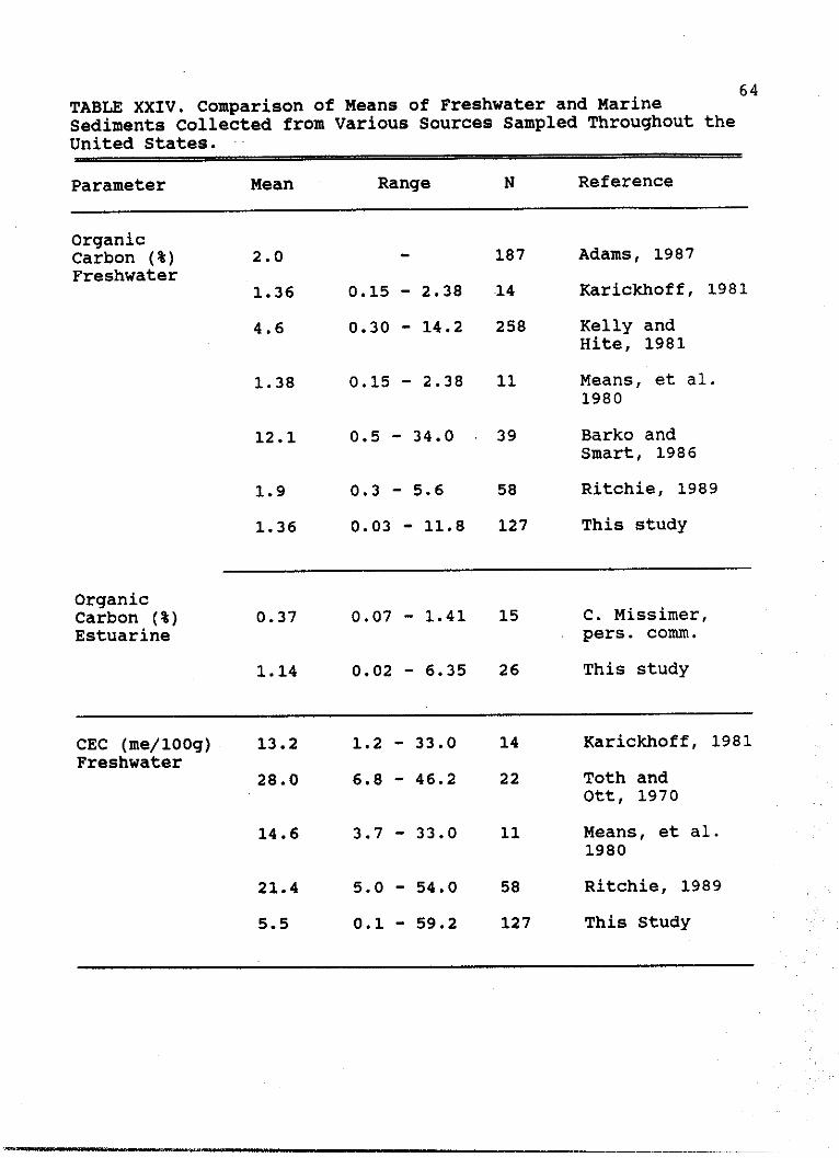
64TABLE XXIV. Comparison of Means of Freshwater and MarineSediments Collected from Various Sources Sampled Throughout theUnited States.
Parameter Mean Range N Reference
OrganicCarbon (%) 2.0 187 Adams, 1987Freshwater
1.36 0.15 - 2.38 .14 Karickhoff, 1981
4.6 0.30 - 14.2 258 Kelly andHite, 1981
1.38 0.15 - 2.38 11 Means, et al.1980
12.1 0.5 - 34.0 39 Barko andSmart, 1986
1.9 0.3 - 5.6 58 Ritchie, 1989
1.36 0.03 - 11.8 127 This study
OrganicCarbon (%) 0.37 0.07 - 1.41 15 C. Missimer,Estuarine pers. comm.
1.14 0.02 - 6.35 26 This study
CEC (me/100g) 13.2 1.2 - 33.0 14 Karickhoff, 1981Freshwater
28.0 6.8 - 46.2 22 Toth andOtt, 1970
14.6 3.7 - 33.0 11 Means, et al.1980
21.4 5.0 - 54.0 58 Ritchie, 1989
5.5 0.1 - 59.2 127 This Study

65
communication). Eighty - eight percent of the OC values
obtained during this study for both freshwater and estuarine
sediments combined were less than 3% OC and 93% of the OC
values collected were less than 5% OC.
Cation exchange capacity (CEC) determined for sediments
in this study was lower than CEC values reported elsewhere.
For samples collected during this study (freshwater and
estuarine combined), 98% of the CEC values were between 0.1
and 35 me/100g. Karickhoff (1981) reported values with a
mean CEC of 13.2 me/100g, while Toth and Ott (1970)
presented a CEC of 28.0 me/100g from 22 sediment samples
collected in the Northeastern U.S. Ritchie (1989) reported a
mean CEC value of 21.4 for sediments from reservoirs
throughout the country. Marine sediments were also reported
(Toth and Ott, 1970) with a mean of 59.7 me/100g for
Chesapeake Bay and Barnagat Bay samples but these samples
were not washed to remove chloride as in the present study.
Samples collected by Means et al. (1980) had a mean CEC of
14.59 me/100g.
CEC values for freshwater sediments (mean = 5.5 + S.D.
= 8.3) were similar to CEC values from estuarine sites (mean
= 3.6 + S.D. = 5.8).
CEC was not observed to be positively correlated with
clay content in this study (Table XIII) probably because the
type of clay material is also important in determining the

66
CEC (Brady,..1974; Toth and Ott, 1970; Bailey and White,
1964). Clay minerals such as vermiculite and montmorillonite
have CEC's ranging from 80 to 150 me/100g and surface areas
ranging from 6 - 8 x 106 cm2/g while clay minerals such as
chlorite and kaolinite have lower CEC's (3 to 40 me/100g)
and lower (7 - 40 x 104 cm2/g) surface areas (Bailey and
White, 1964).
Redox potentials for freshwater and estuarine sediments
on average, indicated reduced sediments (Bohn, 1971) with
freshwater sediments having slightly lower redox potentials
(Tables VI and VII). Sediment redox potential effects on
biodegradation have been noted for some synthetic organics
(Gambrell et al., 1984).
Since particle surface area was observed to vary
several orders of magnitude, it has logical potential as a
sediment toxicant bioavailability normalization factor.
Surface area of soils is reported to be positively
correlated with CEC (r = 0.985) and percent clay (r = 0.918)
(Mortland, 1954). However, surface area was not found to be
correlated to CEC or percent clay in this study (r = -0.136,
N = 370). Particle surface area depends on both size and
shape of sediment particles as well as type and amount of
clay present (Hillel, 1971; Brady, 1974). Clay minerals such
as montmorillonite and vermiculite have surface areas on the
order of 800 m2/g and extensive internal surfaces due to

67
their sheetlike structure. Each particle is made up of
numerous plate-like crystal units with negative charges that
attract cations and water (Brady, 1974). Clay minerals such
as kaolinite have only external surfaces and much lower
surface areas (10 to 70 m2/g) (Hillel, 1971; Bailey and
White, 1964; Carter et al., 1986); thus, the potential for
binding neutral organic chemicals is much greater in
sediments with greater particle surface areas (greater CEC).
Silt and sand particles have particle surface areas on the
order of 0.045 m2/g and 0.0045 m2/g, respectively, and
therefore would be expected to provide relatively few
binding sites for hydrophobic compounds (Karickhoff et al.,
1979).
Percent organic carbon was highly significantly
correlated with CEC and highly negatively correlated with
percent solids and percent sand (Table XIII). Ritchie (1989)
reported that percent OC is positively significantly
correlated with CEC (r = 0.31, p = 0.01, N = 58). Percent OC
was reportedly highly correlated with CEC in other studies
as well (Karickhoff, 1981; Bailey and White, 1964). The
highly negative correlations between OC content and CEC with
sand content (Table XIII) suggest that very little of the OC
is associated with the sand fraction but rather with the
silt and clay fractions. A significant positive correlation
between CEC and percent clay has been noted elsewhere

68
(Mortland, 1954) but was not observed in this study. This is
probably due to the varying types and amounts of clay
minerals present in the sediments collected and because CEC
largely depends on the high surface area clay minerals such
as montmorillonite (Dyal and Hendricks, 1950).
Few studies have focused on effects of OC content or
other sediment characteristics on bioavailability of
potentially toxic materials sorbed to sediments. Staples et
al. (1985) hypothesized that bioavailability of neutral
organic compounds is dependent upon suspended solids
concentration and is a function of organic carbon content
and sorption coefficient (Kp) of the chemical. However,
their data did not support this hypothesis. Adams (1984)
suggested that no-effect concentrations were dependent upon
OC content in sediment studies using Chironomus tentans.
Bioavailability of organic compounds has been linked to
solubility, sediment particle size and OC content of
sediments (Schuytema, et al., 1988). The hypothesis that
sediment toxicity due to a particular chemical does not vary
if OC content is held constant while varying other sediment
characteristics has apparently not been tested until now.
These data now permit experimental examination of this and
other hypotheses relevant to development of scientifically
defensible SQC.

69
Toxicity Testing
The ten day aqueous EC50 value for 3 day old Daphnia
magna exposed to fluoranthene was 102.6 ug/l. Preliminary
testing using <24 h old Daphnia neonates showed a 48 h EC50
of 91.9 ug/l (95% C.I. = 77.4 - 108.3). Previous studies
using p. magna exposed to fluoranthene in 48 h static tests
reported a 48 h EC50 value of 325,000 ug/l (U.S. EPA, 1980)
which is well in excess of the present study's observed
aqueous solubility of fluoranthene (150 ug/1).
The organic carbon normalization approach implies that
the bioavailable fraction of a neutral organic compound
(fluoranthene) in sediment is governed solely or largely by
the total organic carbon content of that sediment.
Theoretically, if the organic carbon content increases, then
the toxicity of fluoranthene should decrease. Conversely, if
organic carbon content of sediment is held constant (as in
this study), then observed toxicity should remain constant.
The objective of this study was to select three sediments
with similar organic carbon contents while varying other
sediment characteristics (Table III). However, by holding
organic carbon content constant, it was difficult to vary
other sediment characteristics by an order of magnitude
while at the same time having a sediment that exhibited no
toxicity to the organisms tested. Since all sediment
characteristics studied were essentially the same, the

70
variance observed between sediments for each organism is due
to factors other than the sediment characteristics examined
in this study.
As illustrated in Figures 5 - 13, significant
differences occurred between sediments for all three
organisms tested for overlying water, pore water, and
sediment fluoranthene concentrations. These data indicate
that bioavailability of fluoranthene to D. magna, H. azteca
and _. tentans is mediated by factors other than sediment
organic carbon content alone. The data also illustrate that
the other sediment characteristics studied did not vary
sufficiently to account for the significant differences
observed between the toxicity mediating properties of the
sediments.
One of the assumptions of the Equilibrium Partitioning
approach to SQC development is that water column organisms
have the same sensitivities as infaunal benthic organisms
(Chapman, 1989). The data from this study of fluoranthene
based on 10 day EC50s (Table XIV) indicate that benthic
species such as C. tentans and bottom dwelling species such
as H. azteca are as sensitive or more sensitive than water
column organisms such as D. magna.
The findings of this study differ from other studies on
the effects of organic carbon on bioavailability of neutral
organic compounds to aquatic organisms. Adams et al. (1985)
%1- 1- ", - -, - -, I l , I I , ,,, .- , , -Wjc . "Immommalopm

71
found that C. tentans was affected biologically only when
the pesticide, Kepone (KP = 120), sediment pore water
concentrations exceeded the chronic water effect level for
Kepone. Adams et al. (1985), and Ziegenfuss et al. (1986)
observed that overlying water concentrations were very
similar to pore water concentrations in static tests using
sediments with varying organic carbon contents. Ziegenfuss
et. al.. (1986) also noted that LC50 values based on pore
water concentrations were the same as those based on
overlying water concentrations. That study supported the
organic carbon normalization theory for neutral organic
compounds sorbed to sediments.
Nebeker et al. (1989) exposed H. azteca to DDT and
endrin in 10 day whole sediment tests. The authors observed
that DDT (KP = 1.2 x 10⁵) was more tightly bound to high
organic carbon content sediment (10.5%) than low organic
carbon sediment (3.0%) and was not bioavailable to Hyalella.
These DDT data supported the organic carbon normalization
approach. However, endrin (KP = 6.9 x 10³) toxicity was
observed not to be affected by sediment organic carbon
content, thus contradicting the organic carbon normalization
approach to SQC development.
Data from this study do not support the organic carbon
normalization approach. Fluoranthene sediment pore water
concentrations were not similar to overlying water

72
concentrations in any of the tests conducted, even though
organic carbon content was held constant. EC50 values based
on sediment pore water concentrations were not similar to
EC50 values based on overlying water concentrations. One of
the major assumptions of the Equilibrium Partitioning
approach is that sediment pore water concentrations can be
calculated directly from the amount of chemical sorbed to
sediments and percent OC (Chapman, 1989). Figure 14
demonstrates that fluoranthene sediment pore water
concentrations vary by up to a factor of four (taking
fluoranthene sediment concentrations into account),
illustrating that fluoranthene sediment pore water
concentrations cannot be accurately calculated from the
amount of fluoranthene sorbed to sediments.
Based on the above discussion, the mediating effects of
organic carbon were not dependent upon the chemicals'
partition coefficient (K). The partition coefficients for
Kepone (K = 120) and DDT (KP = 1.2 x 10⁵) that supported the
EP approach differed by three orders of magnitude. Partition
coefficients of fluoranthene and endrin that do not support
the EP approach were very similar (K = 1 x 10') and were
between the coefficient values for Kepone and DDT. These
data suggest that organic chemical partition coefficients do
not account for the observed differences in toxicity of
organic compounds sorbed to sediments.

73
u..c' +
+
++
0 0 +
*+Pu
0 0 0 8 0 000
(1/5n) (eJod) p e U! eueqluiorqc jo uoequeouoo
4-
. E 0
-'
0
0
co
-4.s
U
0
o -M>4.)0M 4)
0 0
0OH41. a
0 r4-4
0 0
4) Mp 9
0 0
4-).).0
0 H40
~40H
4J 0
0 COH-
H
$Z3z48
U
+
m U
U U *
U n
EuU. U
UU
U m
m

74
One subject that has not been addressed is whether or
not chemical sorption and bioavailability are similarly
affected by differing forms of organic carbon. As noted in
Table VI, coal was found in two sediment samples. Does coal
affect chemical sorption and bioavailability the same as
dissolved and particulate organic carbon? (e.g. - are all
forms of organic carbon created equal?). Answers to these
questions must be addressed in order to develop defensible
SQC.
Conclusions
1) Percent organic carbon, cation exchange capacity and
particle surface area were the only sediment characteristics
studied that varied sufficiently to encompass the range in
observed sediment toxicity.
2) Sediment characteristics studied for both freshwater and
marine sediments (organic carbon, cation exchange capacity,
particle size distribution, particle surface area, redox
potential, and percent sediment solids) were found to be
statistically significantly different within and among most
physiographic provinces.
3) Freshwater sediment characteristics did not differ
significantly from estuarine (marine) sediment
characteristics.

75
4) These data suggest that there is no significant
correlation between sediment toxicity and the bulk chemistry
of sediments (organic carbon, cation exchange capacity,
particle size distribution, particle surface area).
5) Total organic carbon content of sediments varies
sufficiently (two orders of magnitude) to be used as a
potential normalization factor for the bioavailability of
potentially toxic materials in sediments.
6) Sediments with similar organic carbon contents do not
necessarily possess similar toxicity mediating properties
for neutral organic compounds (e.g. fluoranthene).

APPENDIX A
SEDIMENT COLLECTION SUMMARY SHEET
76

1)
2)
- Sediment Collection Summary Sheet
Sediment particle size must be <2 mm diameter.
Sediments should be kept on ice or refrigerated at 40C
if possible - Please Don't Freeze Sediment!
Province:
Site Name:
Town/County/State:
River/Lake/Bay Name:
Highway #:
Date Collected:
Collected By:
Sediment Distingiushing Characteristics (if any):
If you have any questions, please call:
Burton Suedel(817) 565-3599Thank You!
77
4*zAvi*o46,-4Wi ",- , -, -, 4- -,- -,, - -44"J A" -, -

APPENDIX B
SEDIMENT ANALYSIS PROCEDURES
78

79
SEDIMENT DISTRIBUTION FOR EACH PARAMETER
1. Homogenize sediment sample thoroughly with spatula orpower drill and impeller.
2. Sieve sediment through a #10 U.S.A. Standard TestingSieve (2.00 mm opening) to remove particles larger thancoarse sand.
3. Homogenize sediment again to ensure complete mixing.
4. Need approximately 5g wet (X3 reps) in aluminum pansfor percent solids.
5. Need 5.Og wet (X3 reps/sediment) for CEC.
6. Need wet sediment (100 ml) in sample container forredox potential.
7. Need approximately 2g wet (X3 reps) for percent organiccarbon determination (does not need to be weighed).
8. Dry sediment (35g) equivalent for particle size in a200 ml Beaker.
Weigh out wet sediment and divide by percent water(decimal fraction) to obtain dry weight equivalent ofsample.

80
PERCENT SOLIDS (PERCENT WATER)(after Black, 1986)
1. Homogenize sediment sample.
2. Weigh out approximately 5g wet sediment sample on atared aluminum foil dish to the nearest 1.0 mg (3 repsper site). Do not touch aluminum pan with fingers - usetongs.
3. Dry samples approximately 24h in a drying oven at103-105 C.
4. Remove samples from drying oven and let cool in adesiccator. Weigh the samples on the same balanceused to obtain the wet weight.
5. Repeat the drying process until a constant weight isobtained.
6. The total solids of the sediment samples are calculatedby dividing the weight of the dried residue by theinitial weight of the sample:
sed dry wt (after)%Solids =X-----------------------x 100
sed wet wt (before)
% Water = 100 - % Solids
81
CATION EXCHANGE CAPACITY(after Plumb, 1981)
The cation exchange capacity (CEC) of a sediment is ameasure of the reversibly bound cations in the sample, or, ameasure of those cations held on the surface within thecrystalline matrix of some minerals. These cations maypotentially be released to the water column underappropriate conditions.
The procedure consists of equilibrating a sedimentsample with a highly soluble salt solution. The theorybehind the procedure is that the high concentration of asoluble cation will replace the sorbed or bound cationsassociated with the sediment. The replaced cations can thenbe determined individually in the leachate or the sedimentsample can be washed and reequilibrated with a secondsoluble salt. The second leachate is then analyzed fortotal cation exchange capacity. The standard leachate thatis most often used is 1 N ammonium acetate. The principleadvantages of this approach are the pH buffering capacity ofammonium acetate solutions and the relative ease of theammonia determination. However, ammonium acetate may yieldlow results with (a) samples containing 1:1 type clayminerals such as kaolin or halloysite, or (b) highlycalcareous sediments due to the dissolution of calciumcarbonate.
The exchange capacity of a sample is influenced by theclay content of the sample, the type of clay, the organicmatter content, the pH of the displacing solution, thenature and concentration of the displacing cation, and thesediment-to-solution ratio. Since many of these factors areoperationally defined, the CEC of the sample should beconsidered operationally defined. Most techniques will onlyvary the magnitude of the CEC of a sample and not therelative order of a number of samples. Therefore, careshould be taken to standardize as many variables as possible(ammonia concentration, pH, solid-liquid ratio, and time ofcontact) to ensure uniformity and comparability of results.
Sample Handling and Storage
Samples may be collected with any convenient collectiondevice and stored in either glass or plastic containers.Field moist samples should be used for the CEC determinationas the process of drying has been shown to alter the CEC.At this time, the storage time limits are not known. Sincesample oxidation may indirectly affect CEC, it isrecommended that samples be processed as soon as possible.

82
Reagents Needed:
1N NH40Ac: Dissolve 77g of ammonium acetate in Milli Q(MQ) or deionized water (DI) and dilute to 1 liter.
80% ethanol: Mix 80 ml ethanol in 100 ml volumetricflask and dilute to 100 ml with MQ water.
10% NaCl: Dissolve 100g of NaCl in MQ water; dilute to1 liter.
* Note: If marine or brackish sediments are used, wash thesediments with DI water until there is no trace ofchloride.
Procedure:
1. Weigh out a 5.00g sample of homogenized sediment ina 40 ml polypropylene centrifuge tube. Do threereplicates per site.
2. Add 33 ml of 1N NH40Ac solution.
3. Shake sample(s) on a vortex mixer for 15 secondsand let the suspension stand for 30 minutes.
4. Vortex mix the suspension again for 15 seconds.
5. Centrifuge for 5 minutes at 1600 rpm (300 xg).
6. Decant the NH40Ac solution.
7. Repeat 2X (#3-#7)-.
8. Add 33 ml 80% ethanol to the sediment residue inthe centrifuge tube.
9. Vortex mix the tubes.
10. Centrifuge for 5 minutes at 1600 rpm.
11. Decant the ethanol layer and discard (note yellowcolor of ETOH).
12. Repeat 2X (#9-#11).

83
13. Add 33 ml of 10% NaCl solution to the washedsediment residue. Vortex mix.
14. Centrifuge the sample for 5 minutes at 1600 rpm.
15. Decant the liquid phase into a 125 ml erlenmeyerflask.
16. Repeat 2X (#13-#15).
18. Dilute the erlenmeyer flask to volume (100 ml) withNaCl.
19. Analyze the sediment leachate for ammonia.
(X mg/L) (0.1) (100)CEC (me/100g) =-------------------------
(18 mg/meq) (g) (%S)
Where:
X = ammonia concentration in NaCl leachate, mg/L
0.1 = volume of NaCl leachate, liters
18 = millequivalent weight of ammonium ion, mg/me
g = weight of wet sediment sample, grams
%S= percent solids (% dry weight) in sediment sampleas a decimal fraction
84
AMMONIA ANALYSISFOR CATION EXCHANGE CAPACITY DETERMINATION(Standard Methods 15th Ed. pp. 362-363)
The ammonia-selective electrode uses a hydrophobic gas-permeable membrane to separate the sample from an internalsolution. By increasing the pH of the sample to above 11with a strong base, dissolved ammonia is converted to NH3(aq.). This diffuses through the membrane altering the pH ofthe internal solution, which is sensed by a pH electrode.
STORAGE AND MAINTENANCEThe ammonia electrode (Orion Model 95-12) is stored in
0.1M stock standard or the 1000 ppm stock solution. Replacethe storage solution when it becomes colored. The probemembrane must be replaced periodically. The probe manualgives a range of one week to several months, depending onuse. Membranes are expensive and a replacement supplyrequires 3-4 weeks to be filled; so use them judiciously. Toreplace the membrane, unscrew the top cap and remove theinner electrode body, pour out the inner filling solution,remove the bottom cap and the old membrane. Using forceps tohold the edge of the membrane, loosely stretch the membraneacross the bottom of the outer body. Place the cap over theends and screw it on finger-tight. The membrane should bewrinkle-free. Using the syringe, put 2.5 ml of the internalfilling solution (Orion 95-12-02) into the outer body. Placeinner body into the outer body and screw on the upper cap.Shake the fully assembled electrode as if it were a clinicalthermometer. Use an electrode stand that holds the probe ata 200 angle to prevent air entrapment. Prior to runningsamples, warm the ammonia ISA and standard to the sametemperature as the samples to be tested.
Ammonia Stock Standard:3.819 g anhydrous, reagent-grade NH4 C1 (oven dry at 100
+ 50C for 24h) brought to 1000 ml with MQ water. This yieldsa 1000 ppm solution. 1 ml = 1 mg NH3 -N = 1.22 mg NH3
Ammonia ISA (ionic strength adjuster)400 g NaOH in 800 ml ammonia free water (MQ). Cool and
dilute to 1000 ml. This yields 10M NaOH. This ISA does notrequire refrigeration.
SLOPE CHECK - AMMONIA1. Rinse all glassware with MQ water.
2. Warm samples to 200 C by placing them in a warmwater bath. Monitor the temperature by placing athermometer in the mouth of one of the samplebottles.
85
3. Rinse the ammonia probe with MQ water, gently wipewith a Kimwipe and place in a beaker with pH 4buffer.
4. Plug probe into meter (Corning Model 135 pH/ionmeter).
5. Make sure the meter is clear by pressing SLOPE. Ifa number appears press RESET (RESET clears allstored data).
6. Put mode on Mv by pressing MODE button until thered light is next to Mv.
7. Press 0, CAL 1.
8. In a 150 ml beaker rinsed with MQ water add 100 mlof MQ water and 1.0 ml 1000 ppm ammonia stockstandard.
9. Place the beaker on a stir plate, rinse the stirbar with MQ water and place it in the beaker. Stirso as not to have a vortex.
10. Rinse the probe with MQ water, gently wipe andplace in the beaker.
11. Add 1.0 ml ISA (10M NaOH) to the beaker and pressREAD.
12. Press CAL 1 and then CLEAR when the digital readoutremains constant for 4 flashes of the red light.
13. Without removing the probe, add an additional 10 mlof the ammonia stock and press READ.
14. Wait for the numbers to stabilize. The digitalreadout should display -57.00 + 3.
If the readout deviates considerably (less than -60 orgreater than -50), soak the probe in pH 4 buffer for 10minutes, redo the slope check, and see the trouble shooterssection of the ammonia probe users manual.
CALIBRATION1. Press CLEAR.
2. Rinse the ammonia probe with MQ water, gently wipeand place in a small beaker with pH 4 buffer.

86
3. Rinse three volumetric flasks (100 ml) with MQwater and then fill each with approximately 85 mlof MQ water.
4. Add 1.0 ml of the 1000 ppm ammonia stock standardto the volumetric flask marked 10 ppm. Bring tovolume with MQ water, cover with parafilm andinvert several times.
5. Take out 10 ml of the 10 ppm dilution and add it tothe volumeteric flask marked 1.0 ppm. Bring tovolume with MQ water, cover and invert severaltimes.
6. Take out 10 ml of the 1.0 ppm dilution and add itto the volumetric flask marked 0.1 ppm. Bring tovolume with MQ water, cover and invert severaltimes.
7. Rinse two 150 ml beakers with MQ water. Pour theentire contents of the 1.0 ppm dilution into onebeaker and the contents of the 0.1 ppm dilutioninto the other beaker.
Keep separate.
8. Change the mode of the meter to ACTIVITY bypressing MODE until the red light is next toACTIVITY.
9. Press 1.0 CAL 1, 0.1 CAL 2, -60.00 SLOPE.
10. Check by pressing CAL 1, CAL 2, SLOPE.
11. Place the beaker with the 1.0 ppm dilution on thestir plate. Rinse the stir bar and place in thebeaker.
12. Rinse probe, gently wipe and place in the beaker.
13. Add 1.0 ml ISA to the beaker and press READ.
14. When the number stabilizes for 4 flashes of the redlight, press CAL 1.
15. Press CLEAR, remove the probe, rinse and gentlywipe and place it in the pH 4 buffer. Place thebeaker with the 0.1 ppm dilution on the stir plate.Place a rinsed stir bar in the beaker.
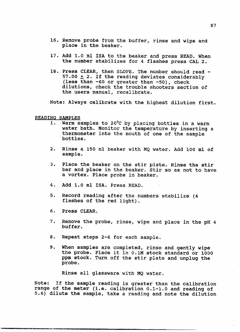
87
16. Remove probe from the buffer, rinse and wipe andplace in the beaker.
17. Add 1.0 ml ISA to the beaker and press READ. Whenthe number stabilizes for 4 flashes press CAL 2.
18. Press CLEAR, then SLOPE. The number should read -57.00 + 2. If the reading deviates considerably(less than -60 or greater than -50), checkdilutions, check the trouble shooters section ofthe users manual, recalibrate.
Note: Always calibrate with the highest dilution first.
READING SAMPLES1. Warm samples to 200 C by placing bottles in a warm
water bath. Monitor the temperature by inserting athermometer into the mouth of one of the samplebottles.
2. Rinse a 150 ml beaker with MQ water. Add 100 ml ofsample.
3. Place the beaker on the stir plate. Rinse the stirbar and place in the beaker. Stir so as not to havea vortex. Place probe in beaker.
4. Add 1.0 ml ISA. Press READ.
5. Record reading after the numbers stabilize (4flashes of the red light).
6. Press CLEAR.
7. Remove the probe, rinse, wipe and place in the pH 4buffer.
8. Repeat steps 2-6 for each sample.
9. When samples are completed, rinse and gently wipethe probe. Place it in 0.1M stock standard or 1000ppm stock. Turn off the stir plate and unplug theprobe.
Rinse all glassware with MQ water.
Note: If the sample reading is greater than the calibrationrange of the meter (i.e. calibration 0.1-1.0 and reading of5.6) dilute the sample, take a reading and note the dilution

88
factor. The meter can also be calibrated to the anticipatedrange of the samples. Recalibration may be necessary.
Note: If reading is below 0.01 then it is below thedetection limit.
STANDARD ADDITION SPIKESome of the samples in the sample run should be
"spiked" to find the range of detection. After the samplehas stabilized, the standard addition spike is placed in thesample and read. The standard addition should not exceed thedetection limit. An example of a standard addition spikefollows:
In a 10 to 1 calibration, a 0.5 ppm spike may be used(1 ml of a 10 ppm standard dilution). This addition shouldincrease the sample reading 0.1 ppm.
89
PARTICLE SIZE
SEDIMENT PARTICLE COMPOSITION ANALYSIS - HYDROMETER METHOD(after Black, 1986)
Particle size distribution is a cumulative frequencydistribution or a frequency distribution of relative amountsof particles in a sample within a specified size range. Thesize of a discrete particle is usually characterized as alinear dimension and designated as a diameter. It should berecognized that the use of sieves and settling tubes willresult in a separation based on particle shape as well asparticle size.
The size distribution of sediments can be of importancebecause it can affect the distribution of chemicals in theaquatic environment. Specifically, sediments can removechemical contaminants from water by the process of sorption.Further, since sorption is a surface phenomena, the smallerparticle sizes generally have a higher concentration ofthese chemical contaminants on a weight/weight basis.
There is a certain amount of arbitrariness associatedwith particle size analysis. One method relies on thetreatment of the sample with hydrogen peroxide to destroyorganic matter that may be causing the sediment particles toaggregate. While this approach will define the trueparticle size distribution of the sample, the results willnot be representative of the surface area potentiallyavailable for sorption or exchange reactions. On the otherhand, sizing of sediments without peroxide treatment wouldyield results more representative of the exposed surfacearea but the apparent particle size distribution may beaffected by the method of sample handling prior to sizing.The latter procedure will be used in this study.
Sample Handling and Storage
Samples scheduled for particle size analysis may bestored in either plastic or glass containers. The samplesshould be chilled at 4-50C but never frozen prior toanalysis. If samples cannot be analyzed within a few hours,Lugols solution should be added as a preservative tominimize the effects of bacterial growth (not used in thisstudy).
The required amount of sediment will range fromapproximately 35 to 45g (dry wt), depending on the sizedistribution. Should the sample contain a large percentageof coarse sand and gravel, a larger sample size should be

90
used to ensure that the smaller size classes are beingrepresentatively sampled.
It is recommended that particle size samples not befrozen or dried prior to analysis. The basis of thisrecommendation is that the freezing-thawing cycle or sampledrying may cause an irreversible change in the particle sizedistribution due to oxidation and/or agglomeration.
Particle size distribution is as follows:
Grade Particle Diameter (mm)
Course sand 0.2 - 2.0
Fine sand 0.02 - 0.2
Silt 0.002 - 0.02
Clay < 0.002
Equipment:
1. Balance - sensitive to 0.01g
2. Hydrometer
3. Several 1 liter graduated cylinders - one blank and 3cylinders/sediment site
4. Thermometer
5. 16,000 rpm blender
6. Timer
7. 250 ml beakers
8. Squirt bottle
9. Sediment plunger
10. n-amyl alcohol

91
Reagents:
Sodium hexametaphosphate (Na 3 PO) 6 (HMP) 5% molalsolution
(w/vol) - 50g HMP weighed out and diluted to 1 literwith deionized (DI) water.
Procedure:
1. Wet sediment sample is sieved to 2 mm particle sizewith a #10 sieve.
2. Place > 45g of wet sediment in a tared 250 ml beaker(X3 reps). Divide target dry weight (35g) by solidsfraction to obtain wet weight needed. Record sedimentweights. Add 100 ml of HMP solution to the samples.Mix thoroughly with a spatula and cover. Allow sedimentto soak in the HMP solution between 15 to 24 hours.
3. Sediment and HMP are then rinsed into a blender(Hamilton Beach, Scovill Model 936.1) with DI water,rinsing beaker with squirt bottle. Fill blender cup toapproximately 1-2 inches from the top with DI water.Blend for 2 minutes on "high" speed.
4. Wash contents of blender cup into a 1 liter graduatedcylinder with DI squirt bottle. Fill cylinder to the 1liter mark with DI water.
5. Prepare blank with 100 ml HMP solution and 900 ml DIwater.
6. Do not use plunger on blank. Read hydrometer on blankfirst. Only one reading is needed on the blank at thebeginning of the run.
7. Agitate sediment column with the plunger for 20complete, even strokes.
8. Immediately after plunging, start timer.
9. If sediment mixture is frothy, add 2-3 drops of n-amylalcohol.
10. Gently place hydrometer into cylinder and prepare totake reading.

92
11. Take readings at 60 sec, 3 min, 15 min, 8 hrs, 24 hrs.
12. Record temperatures at each time period when you canwork them in.
13. Upon removing the hydrometer from each graduatedcylinder, rinse with DI water before placing in nextcylinder.
14. Subtract blank reading from each sample.
15. At the end of the 24 h reading time, sedimentsuspension must be sieved for sands. (Sands settle outtoo quickly to be measured in this analysis).
16. Pour entire contents of graduated cylinder through a#230 sieve (63 um) to separate the sand fraction fromthe silt and clay fractions. Rinse sand well with DIwater to remove HMP and other particles. Use squirtbottle to transfer sand from the sieve into a 250 mlbeaker.
17. Dry sand fraction in a drying oven at less than 1000Covernight so as not to boil water and lose sample.
18. Weigh dry sand fraction.
19. Enter numbers in the computer program as given below.
Target dry sediment weight (approximately 35g) dividedby decimal fraction of percent sediment = amount of wetsediment to weigh out
Wet sediment weight X decimal fraction of percent H20 =equivalent dry sediment weight
Dry sand weight divided by equivalent dry sedimentweight = percent Sand
, .;. - I ., - W W- I I lopm

93
SAS INPUT STATEMENTS TO CALCULATE PARTICLE SIZE DISTRIBUTION
data partsize;input sitename $ sedwt sandwt hydi hyd3 hyd15 hyd480hyd1440 temple temp3 temp15 temp480 temp1440 blank;
sand = (sandwt / sedwt) x 100;clay = 0.0;sedwtrem = (sedwt - sandwt) x 100;
hydl = hydi - blank;hyd3 = hyd3 - blank;hyd15 = hyd15 - blank;hyd480 = hyd480 - blank;hyd1440 = hyd1440 - blank;if hyd480 > hyd1440 then
do;
P1 = (hyd480 / sedwtrem) x 100;P2 = (hyd1440 / sedwtrem) x 100;Sl = (49.664 - (0.29 x (hyd480 + 5))) x (1.3817 -
(0.13 x temp480));S2 = (49.664 - (0.29 x (hyd1440 + 5))) x (1.3817 -
(0.13 x templ440));A = (S1 - 2) / (S1 - S2);B = (P1 - P2);C = A x B;clay = (P1 - C);
end;
silt = 100 - (sand + clay);keep sitename sand silt clay;
*INPUT VARIABLE IDENTIFICATION
sitename = name of sediment sitesedwt = total dry weight of sediment samplesandwt = dry weight of sand fractionhydl = hydrometer reading at 1 minutehyd3 = hydrometer reading at 3 minuteshyd15 = hydrometer reading at 15 minuteshyd480 = hydrometer reading at 8 hourshyd1440 = hyrdometer reading at 24 hourstemple etc. = temperature readings at the designated timesblank = hydrometer reading of blank (900 ml DI water + 100ml HMP)
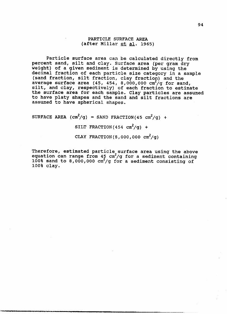
94
PARTICLE SURFACE AREA(after Millar et al. 1965)
Particle surface area can be calculated directly frompercent sand, silt and clay. Surface area (per gram dryweight) of a given sediment is determined by using thedecimal fraction of each particle size category in a sample(sand fraction, silt fraction, clay fraction) and theaverage surface area (45, 454, 8,000,000 cm2/g for sand,silt, and clay, respectively) of each fraction to estimatethe surface area for each sample. Clay particles are assumedto have platy shapes and the sand and silt fractions areassumed to have spherical shapes.
SURFACE AREA (cm2/g) = SAND FRACTION(45 cm2/g) +
SILT FRACTION(454 cm2/g) +
2CLAY FRACTION(8,000,000 cm/g)
Therefore, estimated particle surface area using the aboveequation can range from 45 cm2/g for a sediment containing100% sand to 8,000,000 cm2/g for a sediment consisting of100% clay.

95
PERCENT ORGANIC CARBON(after Dohrmann, 1985)
Carbon may exist in sediment and water samples aseither inorganic or organic compounds. Inorganic carbon ispresent as carbonates, bicarbonates, and possibly freecarbon dioxide. Specific types of compounds that areconsidered to be included in the organic carbon fraction arenonvolatile organic compounds (sugars), volatile organiccompounds (mercaptans), partially volatile compounds (oils),and particulate carbonaceous materials (cellulose).
The basis of the method is the catalytic or chemicaloxidation of carbon in carbon-containing compounds to carbondioxide followed by the quantification of the carbon dioxideproduced. Alternately, the carbon may be reduced to methaneand appropriately quantified. It follows, then, that thedistinction between inorganic carbon and organic carbon isthe method of sample pretreatment. There are presently twoprocedures for determining this separation. one method isbased on sample treatment with a strong acid. This methodis employed in this procedure. Analysis of an untreatedsample is a measure of total carbon while analysis of theacid-treated fraction is a measure of organic carbon.Inorganic carbon is calculated by subtraction. The secondmethod of separation is based on differential thermalcombustion with organic compounds being converted to carbondioxide at 500 0C to 650 OC and inorganic carbon beingconverted to carbon dioxide at 950 C to 1300 0C.
Sample Handling and Storage
Samples should be processed as soon as possible (within24 h if possible) to minimize change due to chemical orbiological oxidation. Atmospheric uptake of carbon dioxideis less critical since it would be evolved when the sampleis acidified prior to analysis. Sediment samples fororganic carbon analysis may be stored in either plastic orglass containers. Air drying of sediments may lead to lowTOC results due to oxidation or volatilization. Therefore,moist storage would be the preferred method of storage.
Sediment Procedure
This is a mini-manual for the Dohrmann DC-80 carbon analyzer(for solids). Excerpt from: Dohrmann DC-80 Total OrganicCarbon Systems Manual.

96
Principle of operation:
A sample placed in a platinum boat is combusted andoxidized at approximately 800 0C in an oxygen atmosphere. Aconstant flow of oxygen carries the resultant C02 to thenon-dispersive infrared detector (NDIR). The NDIR producesan electrical output (peak) which is intergrated and scaledby the number processor and then displayed and printed inmg/kg (ppm) carbon.
I. Sample preparation and start-up:
If TOC is to be measured, the sample must first beacidified to remove inorganic carbon. Place approximately2-3 grams of moist well-mixed sediment in an aluminum dish.Add 1 N H3 PO4 with mixing until pH 2 or less is reached.(Effervescence upon addition of acid indicates inorganiccarbon is being liberated as CO2). Allow to dry overnight at40 C or under a hood. Next day, make a slurry with a smallportion of the dried sediment and MQ water. Check the pH.If sample is at pH 2 or less continue with procedure. If pHis greater than 2 add more acid until a pH 2 or less isreached and allow to dry overnight again. Thoroughly grindand mix dried sediment (including salt crystals that mayhave formed on top) using a mortar and pestle.
Prepare reagents:
20g potassium persulfate (K25208) + 5 ml 1 N H3 PO4 . Bringup to 1 L with MQ water. Use this reagent to fill thereaction vessel.
174 ml of 85% H3 PO4 per liter of MQ water to make 1NH3PO4 .
Check "U" trap tube - add water if necessary.
Prepare standard:
To make 2000 ppm standard: Add 0.425g potassiumhydrogen phthalate (potassium biphthalate) (C.H 5 04 K) and1 ml lN H3 PO4 into 100 ml volumetric flask Bring up to100 ml.
Pour into left sparging vial and then sparge.
Prepare blank:
MQ + approximately 1 ml (to pH < 2.0) 1N H3 PO4 . Spargeon right side.

97
Machine start-up:The detector should be left on at all times; if it isoff, turn on and allow at least a 2 h warm-up.
Turn on POWER, ASM; PUMP off, LAMP off, FURNACE on.Turn on the top box above FURNACE also (MANUAL). Open02 tank valve - regulator should read approximately 45psi. The actual pressure showing on the gauge is notcritical, but the flow rates through the instrument arecritical. Unless one encounters a problem thatjustifies altering the flow, please leave the regulatoras is.
Turn TOC/POC knob to TOC.
Turn range knob to 40 ul.
Change air flow configuration:
Connect "furnace air out" tube to "air in" port on sideof UV reaction module. Connect "furnace air in" to "airout" port. Do this right after turning on furnace.
Allow approximately 30 min to 1 h for stabilizationof baseline (0.0100 + 0.0004) and furnace warm-up (ared glow is a rough indication of approximately 8000C).
II. Calibration:
Place a small piece of quartz wool in a platinum boatthat has been baked to burn off impurities (slide boat intofurnace for 2 minutes or until detecter reading stabilizes).Inject 40 ul (using the yellow-top syringe) of 2000 ppmcarbon standard into the boat, push START, then slide theboat into the furnace. Make sure that all air bubbles havebeen purged from the syringe before shooting into the boat.When the display indicates that the OC peak is on thedownhill side, slide the boat out of the furnace and intoflip top inlet block to cool. Inject another 40 ul of 2000ppm standard. When READY signal beeps, push CALIB as quicklyas possible momentarily . Then run another 40 ul aliquot ofstandard. Analyzer printout should then read 2000 + 40 ppm.Next run 40 ul of acidified blank that has been sparged.Remove quartz wool before running sediment samples.
*If printer reads 'NO CAL' then you have pressed CALIBRATEbutton too slowly. If so, then you must recalibrate byinjecting two or more additional 2000 ppm standards.
I - 1 110 0 1 19

98
III. To run -samples:1) Each OC sediment sample must be ground as fine as
possible using a mortar and pestle.
2) Weigh out 0.01g dried and ground sample into a bakedplatinum boat. You may have to adjust sample size to getreading into 200-4000 ppm range.
3) Each time the door is opened to insert a boat, you mustwait for the atmospheric CO2 peak to clear on thedetecter reading before running another sample.
4) Check baseline before sliding boat into furnace (shouldread 0.01).
4) Slide boat into furnace.
5) Push START.
6) When detector display begins downhill side of peak, pullboat out of furnace into flip top box so it can coolbefore inserting next sample.
7) Do not open flip top boat box until sample has run andthe analyzer beeps!
To turn off analyzer:a) Turn off furnace, ASM, and top box above furnaceb) Turn off gas
IV. To calculate % C:
The carbon analyzer generates a number that is measured inmg/kg (ppm). This number is the Total Organic Carbon presentin the sample. Use this number as [conc] in the equationbelow:
mass of carbon%OC =------------------X 100
mass of sediment
conc (mg/1) (40ul) (1L/1 X 106ul) (lg/1 X 103mg)%OC = -------------------------------------------------X 100
wt of sample (g)

99
(conc) (40/1 X 109)%OC -------------------- X 100
wt of sample
Organic Carbon Procedure - Water Samples
Same as sediment procedure except:
Standards:Make a 100 mg/L standard by taking 5.0 ml of the 2000 mg/Lstock standard into a 100 ml volumetric flask with 1-2 ml 1NH3 PO4 and bring to level with MQ water. This standard shouldread 10 mg/L when injected into the analyzer with a 1 mlsyringe. This std should also read 100 mg/L on the auto-analyzer.
To turn on: Turn on POWER button on top box above furnace.
ASM: POWER on; PUMP on; LAMP on.
Open 02 tank valve.
Range knob set at 1ml.
'Air in' and 'Air out' ports should be connected by the 'U'tube.
Calibrate with 10 mg/L std - everything else as usual.
Acidify each sample with 1ml H3 PO4 before running; acidifyblanks also.
Loading auto sampler:
1) Put first test tube next to rubber ring on the tray (tothe left of the rubber ring).
2) First test tube should be a blank followed by: std, std,3 more blanks, sample, sample2, etc.
3) Use standard and 2 blanks midway through run.
4) At the end of the run use: std, 2 blanks.

100
REDOX POTENTIAL(after Bohn, 1971 and Orion, 1983)
The oxidation-reduction potential (redox potential orEh) is defined as the electromotive force developed by aplatinum electrode immersed in a water or sediment samplerelative to a standard hydrogen electrode or a referenceelectrode of known Eh. The obtained value is a crudeestimate of the oxygen status of the sample. At pH 7.0,oxidized soils are at redox potentials of >400 my,moderately reduced soils about 100 to 400 mv, reduced soils-100 to 100 my, and highly reduced soils -100 to -300 mv.
Sample Collection and Storage
The preferred method of obtaining oxidation-reductionpotential data is in situ measurement. If this isimpractical, the measurements should be made as soon aspossible. Since exposure to the atmosphere may affect theoxidation-reduction potential of the sample (oxygen maydissolve in water or oxidize sediments), precautions shouldbe taken to minimize sample contact with the atmosphereprior to measurement of the oxidation-reduction potential.This precaution will necessitate the use of wet sedimentsamples for the measurement.
Calibration of Redox Electrode
1. Solution A:
Weigh out: 4.22g reagent-grade K4Fe(CN) 6 * 3H20(potassium ferrocyanide)1.65g reagent-grade K3 Fe(CN) 6 (potassiumferricyanide)
Place in a 100 ml volumetric flask. Add approximately50 ml distilled water and swirl to dissolve crystals.Dilute to volume with distilled water.
2. Solution B:
Weigh out: 0.42g potassium ferrocyanate1.65g potassium ferricyanate3.39g potassium fluoride (KF * 2H20)

101
Place in erlenmeyer flask with screw cap, dissolvecrystals and dilute to volume with distilled water.
3. Make sure Markson meter is on standby mode. Insertprobe and adapter into GLASS and REF positionsrespectively on the back of the Markson ElectroMarkAnalyzer.
4. Place probe in solution A flask. Rinse probe withMilli Q water and gently wipe dry with Kimwipe. Placeredox electrode in solution A and turn to mV. Waituntil reading stabilizes. The potential should beapproximately 234 mV. If not, turn STANDARDIZED knobuntil meter reads 234 mV. Lock standardize knob.
5. Rinse electrode with Milli Q water and repeatmeasurement with solution B. Reading should beapproximately 300 mV. If not, turn STANDARDIZED knobuntil meter reads 300 mV.
6. After calibration is complete, rinse electrode withMilli Q water and place in sediment sample. Allowmeter reading to stabilize. This could take 10-15minutes.
7. After reading has stabilized, record reading in mV,remove probe from sample and rinse probe with MQ waterto remove all sediment. Then blot dry with Kimwipe.
8. Repeat steps #6 and #7 for each subsequent sample.
9. After last sediment sample has been run, turn FUNCTIONknob to STANDBY, rinse, dry and remove probe frommeter.
APPENDIX C
ORGANISM CULTURE PROCEDURES
102

103
PROCEDURES FOR MAINTAINING IN-HOUSE DAPHNIA MAGNACULTURES FOR USE IN TOXICITY TESTS
This procedure describes the methods for culturing Daphniamagna for use in toxicity tests. It is based on the methodsdescribed in Biesinger et al. (1987), and Peltier and Weber(1984).
DAPHNIA SOURCE
Daphnia were originally obtained from the U.S. EnvironmentalProtection Agency, Environmental Monitoring SupportLaboratory, Cincinatti, OH.
GENERAL PROCEDURE
Daphnia were maintained in 1000 ml borosilicate glassbeakers containing 800 ml of filtered pond water from theUniversity of North Texas Water Research Field Station(WRFS). New cultures were started once a week with 8neonates (<48 h old) and 800 ml of culture water per beaker.Eight new beakers were started each week. The cultures werefed 2.5 mg/l of a yeast, trout chow, and alfalfa solutiondaily. The culture was maintained in a Precision Model 818illuminated incubator (21 20 C; 50-100 fc; 16h light/ 8hdark). The date of first neonate production was recordedfor each beaker. Neonates were removed and 200 ml of waterwas renewed from the cultures every Monday, Wednesday, andFriday. At that time mortality, neonate production, waterrenewal, and presence of gravid females was recorded foreach culture. Adults were discarded at the end of fourweeks.
CULTURE WATER
Although reconstituted hard water is recommended byBiesinger et al. (1987), D. magna cultures were maintainedusing filtered pond water from the maintenance pond at theUniversity of North Texas WRFS. Natural waters were useddue to the presence of vitamins and nutrients which are notfound in reconstituted hard water. Culture water wasfiltered though a Whatman EPM2000 filter to remove anyparticulate matter or suspended solids and to preventcontamination of the culture by other species of daphnids.

104
FOOD PREPARATION AND FEEDING
The YFA diet is a 500 ml solution consisting of baker'syeast (4.6 g/l), catfish chow (12.6 g/l), and alfalfa (1.0g/l) and deionized water. The mixture was homogenized in atissue blender for five minutes at high speed. The solutionwas then allowed to settle for one hour. After the solutionhad settled, the supernatant (top layer) was saved anddecanted into plastic bottles in 30-50 ml aliquots andfrozen until needed.
CULTURE CONDITIONS
Temperature: 21+20C
Light Quality: Incubator illumination(cool white light)
Light Intensity: 50-100 fc
Photoperiod: 16h light/8h dark
WATER CHEMISTRY
pH: 7.5-8.5
Hardness: 51-192 mg/l
Alkalinity: 120-178 mg/l
Dissolved Oxygen: >40% of saturation
NEONATE REMOVAL (CULLING)
Separating the neonates from the adults is referred to as"culling". The adults were gently pipeted, using a largebore pipet (6mm ID), out of the culture beaker into aholding beaker. The holding beaker contained 50-100 mls offiltered pond water. Care was taken to release the adultsbelow the surface of the water. The neonates in the beakerwere gently poured into a culling chamber. The drain hosewas unclamped and the culture water was drained back intothe original culture beaker. The adults were then pipetedout of the holding beaker and placed back into the originalculture beaker. Care was taken to release the adults belowthe surface of the water in the beaker. Culture water(200ml) was renewed at this point. Polystyrene petri disheswere placed over the beakers to prevent contamination andevaporation.

105
REMOVAL OF NEONATES FOR TOXICITY TESTS
Daphnia (3 days old) used for toxicity tests wereindividually pipeted into a beaker of filtered pond water.Pipetting by hand helped prevent floating that can sometimesoccur when daphnids are transferred by pouring.
STARTING NEW CULTURES
New cultures were started weekly. Eight neonates <48 h oldwere placed in 800 ml of filtered pond water containing 5 mlof YFA solution. Eight beakers were started each week andwere referred to as a "set of cultures" or "row". The dateand the page number were written on each beaker to recordthe age of the daphnids.
ROUTINE MAINTENANCE
Each culture beaker was fed YFA diet daily. Neonates wereculled and 200 ml of culture water was renewed from eachculture beaker on Mondays, Wednesdays, and Fridays. Onceper week, the sides of the beakers were wiped with a Kimpipeto remove algal growth and accumulated food. Daphnids wereexamined for the presence of the first brood. The date ofthe first brood was recorded in the D. magna cultureproduction log. Neonates from the first brood were not usedin tests or used to begin new cultures. Any individualculture beaker which showed mortality >10% per day wasdiscarded. The daphnids were discarded after the fourthweek. Date to first brood, culture number, temperature, DO,pH, conductivity, hardness, and alkalinity were measuredweekly according to Standard Methods (1985).

106
PROCEDURES FOR MAINTAINING IN-HOUSE HYALELLA AZTECACULTURES FOR USE IN TOXICITY TESTS
This procedure describes the methods for culturing Hyalellaazteca for use in toxicity tests. It is based on the methodsdescribed in de March (1981).
HYALELLA SOURCE
Hyalella azteca (Saussure) were originally obtained from theU.S. Fish and Wildlife Service, National FisheriesContaminant Research Center, Columbia, MO.
CULTURE FACILITIES
Amphipod cultures were maintained in 10 gal glass aquariafilled with filtered, dechlorinated tap water. The cultureswere in an isolated room, free of contamination andexcessive disturbances. The cultures were maintained at atemperature of 22+30C and a wide spectrum light intensity ofapproximately 100 f.c. in a 16h light, 8h dark regime.Cultures were vigorously aerated.
Note: If the amphipods come to the surface of the water ormove up the side of the glass, the DO level is too low.Aeration should be increased.
CULTURE WATER
H. azteca cultures were maintained using filtered,dechlorinated tap water. Once per week, half of the water ineach aquarium was siphoned off and replaced with clean,dechlorinated tap water.
SUBSTRATE
Hyalella feed on and live in maple leaves that are placed onthe bottom of the culture aquaria. Fallen maple leaves (Acerspp.) were soaked in aged tap water for 10 days. The leaveswere flushed to remove naturally occurring tannic acidbefore they were placed into the culture aquaria. Leaveswere placed in the aquaria at a depth of approximately 5 cm.Additional leaves were added periodically when the amphipodshad eaten most of the organic portions of the leaves.
FOOD PREPARATION AND FEEDING

107
Hyalella were fed ground Purina Rabbit Chow once per week.Rabbit chow was ground by mixing in a blender at high speedfor 1 minute. Ground pellets were placed in an air-tightcontainer and kept in a freezer until needed.
REMOVAL OF HYALELLA FOR USE IN TOXICITY TESTS
Amphipods were isolated by removing a part of the leaf matfrom a culture aquarium using a 5" fine mesh net. This leafmat was placed on a 1 mm (#18) mesh sieve and dechlorinatedtap water was then gently poured over the leaves to flushthe amphipods into the next sieve (#30) below. The Hyalellawere washed through a #30 sieve (U.S. Standard series, 600um) to obtain animals approximately 3-4 mm in length. Theamphipods were then gently rinsed into a shallow stainlesssteel pan to be transferred to the test beakers. Theorganisms passing through the #18 sieve and trapped by the#30 sieve were used in the toxicity tests.

108
PROCEDURES FOR CULTURING THE MIDGE, CHIRONOMUS TENTANSFOR USE IN TOXICITY TESTS
PURPOSE AND SCOPE
Aquatic safety evaluations of chemicals require conductingtoxicological studies with aquatic organisms in thelaboratory. This procedure provides guidelines onculturing the midge, Chironomus tentans in the laboratoryfor support of a midge aquatic toxicity testing program.
BACKGROUND INFORMATION
It has been recognized that there is a need to includesediment dwelling aquatic organisms when testing chemicalsthat sorb to particulates and bottom sediments.Bioaccumulation studies are often a part of chemical safetyevaluations and require organisms with a relatively largemass to be conducted conveniently. The midge, Chironomustentans (Diptera:Chironomidae), a mosquito-like fly, isrecognized as a useful test organism representing theaquatic benthic community in aquatic safety testing. Theimmature midge (larvae) is worm-like and lives in a casebuilt within soft, flocculent sediments in a variety ofaquatic habitats. Larvae can reach a size of 30 mm inlength and 25 mg wet weight, making C. tentans one of thelarger chironomids. C. tentans is easily cultured in thelaboratory with readily available materials.
QUALITY OF CULTURES
Care was taken in culturing to insure healthy organisms wereavailable for testing. This goal was met by carefullyfollowing the practices that have proven successful (listedbelow).
FACILITIES
Midges were cultured in an isolated area or room, free ofcontamination and excessive disturbances. Water wasmaintained at a temperature of 210 + 20 C and a wide spectrumlight intensity of approximately 100 f.c. in a 16 hourlight, 8 hour dark regime.
MORON

109
CULTURE WATER
C. tentans were cultured in filtered and declorinated tapwater.
CULTURE CHAMBERS
Midges were cultured in 5 to 10 gallon glass aquaria filledwith dechlorinated tap water to a depth of 8 cm. Culturechambers were covered with polyethylene (Saran Wrap) or ascreen to prevent adults from escaping and to exclude otherspecies from entering the cultures. Culture chambers werevigorously aerated with an airstone to maintain asatisfactory dissolved oxygen (DO) concentration.
Note: If the midges come to the surface of the substrate ormove up the side of the glass, the DO level is too low.Aeration should be increased.
MAINTENANCE
Approximately half of the culture water in each aquarium waschanged weekly by using a siphon hose to eliminateaccumulated waste products. While the water level was down,a razor blade was used to scrape the sides of the aquariumto remove fungus and algae. Care was taken to avoidsiphoning too much water before cleaning. Fresh water wasadded slowly to prevent excessive turbulence. Pupal casings,dead adults, etc. were picked out on a regular basis inorder to maintain water quality between water changes.
MIDGE SOURCE
The midges used in the UNT Water Research Field StationAquatic Toxicology Lab were obtained from the Monsanto Co,St. Louis, Mo.
SUBSTRATE
C. tentans requires a substrate in which to construct acase. Brown shredded paper towels have been found to bewell suited for this purpose. Bleached towels are not a goodsubstrate. Strips cut from #1052.5 Industrial Crown-Zellerback (Nibroc) brown paper towels were soaked overnightin acetone to remove impurities. The towels were thenboiled in three changes of tap water until all acetone wasremoved. A tissue blender was then used to shred the towelsinto a pulp. Care was taken to avoid overblending and
"A 0 11114141;1

110
possible shortening of the wood fibers in the pulp. Beforebeing added to the culture, the paper towels were rinsedtwice with dechlorinated tap water to remove extremely smallfibers. The paper pulp was placed into the water of aculture chamber until a depth of 3 cm was obtained. Extraclean paper pulp material was refrigerated until needed.From time to time, new pulp was added to establishedcultures to replace used pulp.
FOOD PREPARATION AND FEEDING
C. tentans is primarily a filter feeder drawing foodparticles into its case from the water column. A suspensionof "Tetra Conditioning Food Vegetable Diet" has been usedwith good success. Fifty grams of fish flake was added to500 ml of dechlorinated tap water and mixed with a tissueblender for 5 minutes. The mixture was then sieved through a#230 stainless steel sieve. The mixture was allowed tosettle overnight. The midges were fed the upper layer onlyas the bottom layer tends to be high in BOD's. Extra foodwas frozen until needed. Portions in use were refrigeratedbetween feedings. For optimal growth of the culture, larvaewere fed daily. The midges were fed 1.0 ml of the Tetrasuspension twice per day. If the water was not clear in 3 or4 hours after feeding, too much food was added. Overfeedingwill lead to the growth of fungi in the aquaria and willnecessitate more frequent water changes.
MIDGE LIFE CYCLE
C. tentans egg masses hatch in 2 to 3 days after depositionin water at temperatures of 19 to 220 C. Larval growth occursin 4 instars of approximately one week each. Under optimalconditions, some larvae will develop into adults 24 to 28days after egg deposition. Adults emerge from pupal casesover a period lasting several weeks. Adult males are easilydistinguished from females in that they have large, plumoseantennae and a much thinner abdomen with visible genetalia.Egg masses are removed from the tanks four days beforelarvae are needed for testing and placed in 20 ml of aged,filtered and dechlorinated tap water. Eggs can be stored ina refrigerator to retard development but after 4 or 5 days,viablity is greatly reduced.

111
CULTURE LOGISTICS
Each egg mass contains from 300 to 500 eggs. Two or threeegg masses laid gently on the substrate is enough to start aculture chamber. A culture chamber may be productive forseveral months and can be expected to produce a few adultseach day once generations of larvae are staggered. Once aculture becomes unproductive because of worn out substrateor contamination by other detrimental organisms, it shouldbe disposed of and a new culture started. Several culturesof different ages should be maintained at any one time asa hedge against unfavorable occurances.

APPENDIX D
ORGANISM TESTING PROCEDURES
112
4A"eAsWtVAW- W --I
113
PROCEDURES FOR CONDUCTING STATIC CHRONIC WHOLE SEDIMENTTOXICITY TESTS WITH
DAPHNIA MAGNA
SCOPE
This procedure describes the methods used by the UNT WaterResearch Field Station (WRFS) Aquatic Toxicology Laboratoryfor obtaining laboratory data to evaluate adverse effects ofcontaminants in whole sediment tests. This method isdesigned to assess the toxic effects of fluoranthene onDaphnia magna survival in 10 day whole sediment exposures instatic systems. Modification of these procedures may bejustified by special needs. Comparison of results obtainedusing modified versions of these procedures might provideuseful information on new concepts and procedures forconducting toxicity tests with Daphnia magna.
This document is to be viewed as a supplement to Peltier andWeber (1985), and Beisinger, et al. (1987).
FACILITIES
Tests were conducted in temperature and light controlledincubators (Precision Model 818). Temperature wasmaintained at 20 +1C with a 16h light, 8h darkphotoperiod.
TEST CHAMBERS
Tests were conducted in 250 ml borosilcate glass beakers andcovered with polystyrene petri dishes to prevent airborncontamination.
FILTRATION
Test water was vacuum filtered through Whatman EPM2000filters to remove large particles, suspended solids, andcontaminant organisms naturally occurring in the pond water.
CLEANING
Test beakers and other equipment which came into contactwith fluoranthene (Flu) was properly washed before each use.All glassware and equipment was first rinsed with deionized

114
water followed by one rinse with reagent grade acetone.Final rinse was with HPLC grade hexane. All glassware wasdried thoroughly before use.
DILUTION WATER
Dilution water was uncontaminated and of consistant quality.All water used in testing was obtained from the WRFSmaintenance pond.
CHARACTERIZATION
Dissolved oxygen, pH, hardness, alkalinity, and conductivitywere measured on day 0 and day 10 of each definitive test.Dissolved oxygen was measured more frequently if <40% ofsaturation.
TEST ORGANISMS
All daphnids were as uniform as possible in age and sizeclass. D. magna neonates (3 days old) were used in thetoxicity tests.
DAPHNIA SOURCE
All daphnids used in testing were from the same source.Daphnia used in WRFS tests were obtained from in-housecultures.
EXPERIMENTAL DESIGN
Screening TestsScreening tests were used to determine whether or not thesediments exhibited background toxicity to the daphnids.Five replicates (beakers) were used with ten Daphnia perreplicate. Test duration was 10 days. Each screening testwas conducted as closely as possible to the definitive testconditions to reduce variability.
Range-Finding TestsRange-finding tests were used to determine the range ofconcentrations of Flu to be used for the definitive testsbecause little was known of the toxicity of fluoranthene(Flu). Range-finding tests had five or more concentrationsspanning one or more orders of magnitude. There was only one

115
replicate and ten daphnids per concentration. Test durationwas 10 days. Test conditions were the same as for thedefinitive tests.
Definitive TestsThe definitive tests consisted of a sample of daphnidsexposed for 10 days to a series of Flu concentrations. Thesetests were used to estimate the EC50 which was the Fluconcentration required to produce an effect (mortality) to50% of the daphnids at the end of 10 days. Test vessels were250 ml borosilicate glass beakers. Six sedimentconcentrations and a control were used per sediment withthree replicates per concentration.The sediment was homogenized first with a power drill andstainless steel impeller. Forty ml of wet sediment wasmeasured in a 50 ml beaker and placed into a 250 ml testbeaker. The test beakers were gently shaken to facilitatesettling of the sediment. For range-finding and definitivetests, the fluoranthene was added to the sediment asdescribed in Appendix F. After sediment spiking wascompleted, 160 ml of WRFS pond water was carefully added bytilting the beaker and pouring the pond water down the sideof the beaker. Test beakers were left to settle overnightbefore adding Daphnia (this is Day -1). The following day,ten daphnids were placed gently into each beaker (this isDay 0). After adding the daphnids to the test beakers, thebeakers were covered with polystyrene petri dishes. Eachbeaker contained 40 ml of wet homogenized sediment and 160ml of WRFS pond water. Test beakers were not aerated duringthe test.
Test TerminationAfter the water samples were removed from the test beakers,the overlying water containing the daphnids was pouredthrough a 500 um mesh stainless steel sieve. The Daphniawere large enough to be trapped by the sieve and were theneasily counted.
ANALYSES
WATER ANALYSIS
A 3 ml sample of the overlying water was extracted from eachtest beaker in range-finding and definitive tests on Day 0and Day 10 and analyzed on a spectrophotofluorometer (SPF)as described in Appendix E.
116
SEDIMENT ANALYSIS
A 1.00 gram sample of sediment was extracted from each testbeaker on Day -1 and Day 10 in range-finding and definitivetests and analyzed on an SPF as described in Appendix E.
INTERSTITIAL WATER ANALYSIS
For definitive tests only:On day 10, all the sediment from one replicate of eachconcentration was placed in a 40 ml centrifuge tube andcentrifuged for 10 minutes at 300 (xg) and subsequentlyanalyzed on an SPF as described in Appendix E.
TEST ENDPOINTS
The endpoint for this study was survival after 10 days.Total neonate production was also recorded at Day 10.
WATER CHEMISTRY
TemperatureThe temperature range for testing was 20+2oC. Temperaturewas monitored daily.
DO did not drop below 40 percent of saturation except inTrinity River tests. Measurements were made at the beginningof the test and as needed thereafter if DO <40 % ofsaturation. Conductivity, pH, alkalinity, hardness weremeasured at the beginning of the test and at testtermination.
FEEDING
D. magna were fed 2 drops of the YFA diet on days 0, 2, 4,6, and 8.
AERATION
No aeration was used during the study.

117
TEST ENDPOINTS
EC50 - Immobility was defined as the inability of thedaphnids to swim or hop off the bottom of the beaker underits own power. Daphnids were observed for 10 seconds.

118
PROCEDURES FOR CONDUCTING STATIC CHRONIC WHOLESEDIMENT TOXICITY TESTS WITH HYALELLLA AZTECA
SCOPE
This procedure describes the methods used by the UNT WaterResearch Field Station (WRFS) Aquatic Toxicology Laboratoryfor obtaining laboratory data to evaluate adverse effects ofcontaminants in whole sediment tests. This method isdesigned to assess the toxic effects of fluoranthene (Flu)on Hyalella azteca survival in 10 day whole sedimentexposures in static systems. Modification of theseprocedures may be justified by special needs. Comparison ofresults obtained using modified versions of these proceduresmight provide useful information on new concepts andprocedures for conducting toxicity tests with Hyalellaazteca.
FACILITIES
Tests were conducted in temperature and light controlledincubators (Precision Model 818). Temperature was maintainedat 20+10C with a 16h light, 8h dark photoperiod.
TEST CHAMBERS
Tests were conducted in 250 ml borosilicate glass beakersand covered with polystyrene petri dishes to prevent airborncontamination.
FILTRATION
Test water was vacuum filtered through Whatman EPM2000filters to remove particles, suspended solids, andcontaminant organisms naturally occurring in the pond water.
CLEANING
Test beakers and other equipment which came into contactwith Flu was properly washed before each use. All glasswareand equipment was first rinsed with deionized water followedby one rinse with reagent grade acetone. Final rinse waswith HPLC grade hexane. All glassware was dried thoroughlybefore use.

119
DILUTION WATER
Dilution water was uncontaminated and of consistant quality.All water used in testing was obtained from the WRFSmaintenance pond.
CHARACTERIZATION
Dissolved oxygen, pH, hardness, alkalinity, and conductivitywere measured on day 0 and day 10 of each definitive test.DO was measured daily if below 40% saturation.
TEST ORGANISMS
All amphipods were as uniform as possible in age and sizeclass. The largest amphipods to pass through a 1mm meshstainless steel screen but fail to pass through a 600 ummesh stainless steel screen were used for testing.
SOURCE
All Hyalella used in testing were obtained from in-housecultures.
EXPERIMENTAL DESIGN
Screening TestsScreening tests were used to determine whether or not thesediments exhibited background toxicity to the amphipods.Five replicates (beakers) were used with ten amphipods perreplicate. Test duration was 10 days. Each screening testwas conducted as closely as possible to definitive testconditions to reduce variability.
Range-Finding TestsRange-finding tests were used to determine the range ofconcentrations of Flu to be used for the definitive testsbecause little was known of the toxicity of Flu. Range-finding tests had five or more concentrations spanning oneor more orders of magnitude. There was only one replicateand five amphipods per concentration. Test duration was 10days. Test conditions were the same as for the definitivetests.
Definitive TestsThe definitive tests consisted of a sample of amphipodsexposed for 10 days to a series of Flu concentrations. Thesetests were used to estimate the EC50 which was the Fluconcentration required to produce an effect (mortality) to
,V-Pwqw Now

120
50% of the Hyalella at the end of 10 days. Test vessels were250 ml borosilicate glass beakers. Six sedimentconcentrations and a control were used per sediment withthree replicates per concentration.
The sediment was homogenized first with a power drill andstainless steel impeller. Forty ml of wet sediment wasmeasured in a 50 ml beaker and placed into a 250 ml testbeaker. The test beakers were gently shaken to facilitatesettling of the sediment. For range-finding and definitivetests, the Flu was added to the sediment as described inAppendix F. After sediment spiking was completed, 160 ml ofWRFS pond water was carefully added by tilting the beakerand pouring the pond water down the side of the beaker. Testbeakers were left to settle overnight before adding theamphipods (this is day -1). The following day, ten Hyalellawere placed gently into each beaker (this is day 0). Afteradding amphipods to the test beakers, the beakers werecovered with polystyrene petri dishes. Each beaker contained40 ml of wet homogenized sediment and 160 ml of WRFS pondwater. Test beakers were not aerated during the test.
Test TerminationAfter the water samples were removed from the test beakers,the overlying water containing the amphipods was pouredthrough a 500 um mesh stainless steel sieve. Amphipods werelarge enough to be trapped by the sieve and were then easilycounted.
WATER CHEMISTRY
TemperatureThe temperature range for testing was 20+10C. Temperaturewas monitored daily.
DO did not drop below 40 percent of saturation except inTrinity River tests. Measurements were made at the beginningof the test and as needed thereafter if DO was below 40%saturation.Conductivity, pH, alkalinity, hardness were measured at thebeginning of the test and at test termination.
WATER ANALYSIS
A 3 ml sample of the overlying water was extracted from eachtest beaker in range-finding and definitive tests on Day 0and Day 10 and analyzed on a spectrophotofluorometer (SPF)as described in Appendix E.

121
SEDIMENT ANALYSIS
A 1.00 gram sample of sediment was extracted from each testbeaker on Day -1 and Day 10 in range-finding and definitivetests and analyzed on an SPF as described in Appendix E.
INTERSTITIAL WATER ANALYSIS
For definitive tests only:On Day 10, all the sediment from one replicate of eachconcentration was placed in a 40 ml centrifuge tube andcentrifuged for 10 minutes at 300 (xg) and subsequentlyanalyzed on an SPF as described in Appendix E.
FEEDING
Amphipods were fed 0.001g of ground Purina Rabbit Chow onDay 0 and Day 5 of the test.
AERATION
No aeration was used during the tests.
TEST ENDPOINTS
EC50 - Mortality. Mortality was defined as no amphipodmovement when sieved at test termination (healthy amphipodsmove quite rapidly when poured on a sieve). Dead Hyalellausually curl up in the shape of a half moon and turn awhitish color when dead.

122
PROCEDURES FOR CONDUCTING STATIC CHRONIC WHOLE SEDIMENTTOXICITY TESTS WITH THE MIDGE,
CHIRONOMUS TENTANS
PURPOSE AND SCOPE
This sediment testing method is a guideline for testingsediments with midges in a static system. The principalobjective is to assess potential toxicity of contaminantsassociated with sediments collected from the field ortoxicant spiked in the laboratory. Procedures are describedfor obtaining laboratory data concerning the chronic effectof contaminants associated with the solid phase of sedimentto midges.
TEST ORGANISM
Chironomus tentans Fabricius (Chironomidae, Diptera) is therecommended test species due to its ease of culturing,relatively large size as second instar larvae, short timerequired to raise larvae to second instar, and ease ofhandling the larvae. This species is widely distributedthroughout the U.S. and spends the larval portion of itslife cycle in a tunnel or case within the upper sedimentlayer of lakes, rivers and estuaries. Its feeding habitsinclude both filter feeding and ingesting sediment.
PROCEDURES
Preliminary PreparationsThe life cycle of C. tentans takes approximately 24-28 daysto complete at 250C. Adult midges are collected in 250 mlflasks where they mate overnight. Egg masses, eachcontaining 300-500 eggs, are isolated in 50 ml beakerscontaining dechlorinated tap water following deposition. Thelength of time from oviposition to hatch is approximately 3-4 days at 23*C. On Day 4 newly hatched larvae aretransferred to isolation chambers (12xl3x2Ocm) containingshredded paper towel substrate, Tetra Conditioning Food anddechlorinated tap water which is aerated through a Pasteurpipet. By Day 10 the larvae have reached the second instarstage of development and are ready for use in sedimenttests. To remove the midges and bring them to the surface ofthe isolation chamber, stir vigorously using a circularmotion with a spatula or hollow glass pipet.

123
TEST FACILITIES
Tests were conducted in temperature and light controlledincubators (Precision Model 818). Temperature was maintainedat 20+10C with a 16h light, 8h dark photoperiod.
TEST WATER
Test water was uncontaminated and of consistant quality. Allwater used in testing was obtained from the WRFS maintenancepond.
EXPERIMENTAL DESIGN
Screening TestsScreening tests were used to determine whether or not thesediments exhibited background toxicity to the midges. Fivereplicates (beakers) were used with five midges perreplicate. Test duration was 10 days. Each screening testwas conducted as closely as possible to the definitive testconditions to reduce variability.
Range-Finding TestsRange-finding tests were used to determine the range ofconcentrations of fluoranthene (Flu) to be used for thedefinitive tests because little was known of the toxicity ofFlu. Range-finding tests had five or more concentrationsspanning one or more orders of magnitude. There was only onereplicate and five midges per concentration. Test durationwas 10 days. Test conditions were the same as for thedefinitive tests.
Definitive TestsThe definitive tests consisted of a sample of midges exposedfor 10 days to a series of Flu concentrations. These testswere used to estimate the EC50 which was the Fluconcentration required to produce an effect (mortality) to50% of the midges at the end of 10 days. Test vessels were250 ml borosilicate glass beakers. Six sedimentconcentrations and a control were used per sediment withthree replicates per concentration.
The sediment was homogenized first with a power drill andstainless steel impeller. Forty ml of wet sediment wasmeasured in a 50 ml beaker and placed into a 250 ml testbeaker. The test beakers were gently shaken to facilitatesettling of the sediment. For range-finding and definitivetests, the Flu was added to the sediment as described inAppendix F. After sediment spiking was completed, 160 ml of
low""
124
WRFS pond water was carefully added by tilting the beakerand pouring the pond water down the side of the beaker. Testbeakers were left to settle overnight before adding themidges (this is Day -1). The following day, five chironomidswere placed gently into each beaker (this is Day 0). Afteradding midges to the test beakers, the beakers were coveredwith polystyrene petri dishes. Each beaker contained 40 mlof wet homogenized sediment and 160 ml of WRFS pond water.Test beakers were not aerated.
Test TerminationAfter the water samples were removed from the test beakers,the overlying water was poured through a 500 um meshstainless steel sieve. If the midges were still in thesediment, the top layer of sediment was rinsed with a squirtbottle containing deionized water (DI) and poured throughthe sieve. This procedure was repeated until all midges wereremoved from the sediment. Midges were large enough to betrapped by the sieve and were then easily counted.
FEEDINGMidges were fed 2 drops of Tetra Conditioning Foodsuspension every other day starting with Day 0.
TEST ENDPOINTSThe endpoint for this study was survival after 10 days.Mortality was defined as complete immobilization and lack ofbody movement upon gentle prodding.
WATER CHEMISTRY
TemperatureThe temperature range for testing was 20+10C. Temperaturewas monitored daily.
DO should not drop below 30 percent of saturation. If so, itwas monitored daily. Measurements were made at the beginningof the test and as needed thereafter. Conductivity, pH,alkalinity, and hardness were measured at the beginning ofthe test and at test termination.
WATER ANALYSIS
A 3 ml sample of the overlying water was extracted from eachtest beaker in range-finding and definitive tests on Day 0
--- l

125
and Day 10 and analyzed on a spectrophotofluorometer (SPF)as described in Appendix E.
SEDIMENT ANALYSIS
A 1.00 gram sample of sediment was extracted from each testbeaker on Day -1 and Day 10 in range-finding and definitivetests and analyzed on an SPF as described in Appendix E.
INTERSTITIAL WATER ANALYSIS
For definitive tests only:On Day 10, all the sediment from one replicate of eachconcentration was placed in a 40 ml centrifuge tube andcentrifuged for 10 minutes at 300 (xg) and subsequentlyanalyzed on an SPF as described in Appendix E.

APPENDIX E
SEDIMENT SPIKING PROCEDURE USING FLUORANTHENE
126

127
SEDIMENT SPIKING PROCEDURE USING FLUORANTHENE
1) In a 50 ml volumetric flask, add 0.500 g of fluoranthene(Flu) (Aldrich Chemical Co.; Cat. #F80-7) and bring tovolume with optima grade acetone. Invert several times tomix. This makes a 10,000 mg/L Flu stock solution that willbe used to spike the sediments.
Note: 1 ul of stock solution = 10 ug of Flu
2) Once 40 ml of sediment was placed in the test beakers,the sediment was ready to be spiked. The Flu - acetonemixture was added to the wet sediment by a ul syringe(Hamilton Co., Reno Nevada). Since very little acetone wasadded to the sediment, the acetone evaporated very quicklyupon contact with the sediment (within 3 min.) and leftbehind crystalline Flu which could then be mixed.
3) Sediment and Flu then mixed for approximately 1 min.using a stainless steel spatula.
4) After mixing, the Day -1 sediment sample was taken andthen the overlying water was added.

APPENDIX F
SPECTROPHOTOMETRIC ANALYSIS OF FLUORANTHENE
128

129
AMINCO-BOWMAN
MODEL # 4-8202 SPF
SPECTROPHOTOFLUOROMETER (SPF)
FLUORANTHENE ANALYSIS
IN WATER
Note: This procedure is a condensed version of the Aminco-Bowman (June, 1976) SPF operator's manual. Consultmanual for further information on the operation ofthis instrument.
A. Turning SPF on:
1. Turn switch on back of SPF on. Make sure blowercomes on.
2. Turn xenon lamp power supply switch on, wait 20sec., then push red starter button and hold about 2sec. (You can look at the back of the SPF and seelight coming on.)
3. Turn on ratio photometer by pushing power on button.
4. Turn H.V. control to manual, adjust current to 0.75max (knob next to H.V. control).
Allow SPF to warm up for 30 min.
B. To zero the SPF.
1. Place blank (solvent) in a 1 cm x 2 cm quartz glasscuvette. Be sure to use the solvent the standardsare dissolved in as a blank. Fluoranthene standardswill use hexane as a solvent. (Make sure emissionshutter is closed before removing the cell chambercover. The rod should be in the up position.)
2. Turn sensitivity to zero adjust. Open emissionshutter (down position).
3. Adjust to zero with zero adjust knob.
4. Turn sensitivity to 0.1.
130
5. With blank subtract on low, adjust to zero with theinner knob on the blank subtract knob.
6. Repeat steps 3, 4, 5 several times until the meterstays on zero.
C. Setting full scale to scan for unknown samples.
1. Close emission shutter and replace blank withstandard.
2. Open emission shutter.
3. Using the excitation dial, select an excitationwavelength on the lower end of the scale.
* When setting excitation and emission wavelengths,always turn the dial to a setting above the desiredwavelength and then slowly turn back.
4. Set the sensitivity switch to 3.
5. Place chart paper on chart recorder and release pen.
6. Turn monochromator switch to emission. (Theinstrument will scan all emission wavelengths for aresponse.)
* Be sure the pen lines up on the chart paper with thesettings on the emission wavelength dial. Adjustthe horizontal control on the chart recorder whilethe dial is moving.
7. Once the instrument has scanned the full range ofwavelengths, the pen will return to the left side ofthe chart paper. At this point, turn themonochromator switch to off.
8. Increase the excitation wavelength by 100 and repeatsteps 6 and 7.
9. Repeat step 8 until you bracket the response curve.
10. The excitation wavelength is the setting on theexcitation dial that gave the greatest response.
11. The emission wavelength is the setting on theemission dial that gave the greatest response.
.,Mw. Eli"
131
12. Set the instrument and the excitation and emissionwavelengths desired.
13. With the sensitivity vernier adjust meter to 100relative intensity. (If 100 relative intensity canbe reached, lower sensitivity.)
Note: Always remember to close emission shutter when thecell chamber is open and to open the emission shutter whentaking a measurement.
D. Setting scale for known samples.
1. Close emission shutter and replace blank withhighest concentration standard.
2. Open emission shutter.
3. Using the excitation dial, select the excitationwavelength for the known sample. Fluoranthene hasan excitation wavelength of 354 nm.
* When setting excitation and emission wavelengths,always turn the dial to a setting above the desiredwavelength and then slowly turn back.
4. Using the emission dial, select the excitationwavelength for the known sample. Fluoranthene hasan emission wavelength of 464 nm.
5. With the sensitivity vernier adjust meter to 100relative intensity. (If 100 relative intensity canbe reached, lower sensitivity.)
Note: Always remember to close emission shutter when thecell chamber is open and to open the emission shutter whentaking a measurement.
6. Repeat steps 1 through 4 using lower standards andrecord relative intensity for each to establish acurve. Do not move the sensitivity vernier once itis set with the highest concentration standard.
E. READING SAMPLES
1. Place sample in cuvette.
2. Open emission shutter.
3. Read relative intensity.

132
4. Close emission shutter.
5. Remove sample.
Note: To determine concentrations of samples, a standardcurve must be established.
F. To shut SPF off.
1. Turn H.V. control off.
2. Turn ratio photometer off.
3. Turn xenon lamp switch off.
4. After light has been off for about 2 min., turn SPFoff.
G. Precautions
1. Use H.V. on manual only
2. Make sure shutter is closed when taking readings.
3. Don't look at light in cell when using the U.V.
4. Don't change any slit or mirror settings unless youknow how and why. If you do change settings, returnthem to the way you found them when you are finishedwith samples.
5. Select a solvent which is invisible at theexcitation and emission wavelengths selected.
H. Fluoranthene standards.
1. Fluoranthene (98%) stock is obtained from AldrichChemical Company (Cat # F80-7).
2. HPLC grade hexane is used as a solvent.
3. Standards of 200, 150, 100, 50, and 10 ug/L areprepared and stored in amber bottles at roomtemperature.,
4. New standards should be prepared monthly.

133
I. Fluoranthene standard curve
1. A standard curve must be established using the 200,150, 100, 50, and 10 ug/L standards. Standards aremeasured according to the procedure listed insection E.
2. Plot a regression of the actual intensity (AI) ofeach standard versus nominal concentration of thestandard.
3. Actual intensity is calculated by multiplying therelative intensity (RI)(taken directly from theratio photometer) by the sensitivity setting (SENS).Actual intensity is then multiplied by the slope ofthe standard curve plus the Y intercept of the lineto obtain the concentration of FLU in ug/L:
RI x SENS x SLOPE + Y INTERCEPT = CONC FLU (ug/L)
4. The slope of the line is calculated by entering thenominal FLU concentrations as 'Y' values andentering the corresponding actual intensities as the'X' values on a calculator or PC BASS linearregression program.
5. A typical example follows:
NOM. CONC. RI x SENS = AI x SLOPE = ug/L
200ppb 100 0.3 30 6.67 200150 75 0.3 22.5 6.67 150100 50 0.3 15 6.67 10050 25 0.3 7.5 6.67 5010 5 0.3 1.5 6.67 10
The slope for the above situation is 6.67 and the Yintercept is zero.
Note: If the hexane/test water ratio is not 1:1 (eg.6 ml pond water and 3 ml of hexane) then this must beaccounted for in calculating the fluorantheneconcentration in the following manner:
mls hexaneRI x SENS x AI x SLOPE + INTERCEPT x----------- = ug/L FLU
mls water
'A" - - -- 4-Q

134
- AQUEOUS PHASE FLUORANTHENE
EXTRACTIONS FOR USE ON A
SPECTROPHOTOFLUOROMETER (SPF)
1) Pipet out 3.0 ml of overlying water from the test vessel(250 ml beaker) into a 16 x 150 mm test tube with ateflon lined screw cap.
2) Filter each 3 ml sample with a Whatman EPM2000 filterusing a 20 ml syringe and Millipore 2 Swinnex-13 filterholder.Filter paper can be cut to size by using a 13 mm corkborer.One filter can be used for all replicates within aconcentration (usually 3 to 5 reps).
3) After filtering, add 3.0 ml HPLC grade hexane to eachtest tube.
4) Screw cap on tightly and then mix each sample on avortex mixer (Thermolyne Type 16700) for 30 seconds.
5) Let tubes set for a few minutes to allow layers to fullyseparate.
6) To run samples on SPF:Remove hexane (top layer) from the test tube with apasteur pipet and place into the cuvette.
Note: By filtering the pond water sample as in Step 2 aboveyou remove the particulate matter in the water. Thereforethe amount of FLU that is read on the SPF would be the totalamount of free FLU in the water and not the total amount ofFLU. The free FLU is the amount that the organism comes incontact with in the water column.

135
INTERSTITIAL (PORE) WATER FLUORANTHENE
EXTRACTIONS FOR USE ON A
SPECTROPHOTOFLUOROMETER (SPF)
1) Upon test completion, remove all test organisms andoverlying water from the test beaker. With a large bladespatula, remove all the sediment from the beaker into a40 ml centrifuge tube. Tap the tube gently on a countertop to ensure complete sediment settling in the tube.
2) Centrifuge sediment for 10 minutes at 300 (xg) (1600RPM's) to obtain approximately 3 to 4 mls of pore water.
3) Carefully pipet out 2 ml of the pore water and placeinto a 20 ml test tube.
4) Filter each 2 ml sample with a Whatman EPM2000 filterwith a filter holder and 20 ml syringe.
5) Screw on test tube cap tightly and vortex mix for 30seconds.
6) Let test tubes set for a few minutes to allow layers tofully separate.
7) To run samples on SPF:
Remove hexane (top layer) from the test tube with apasteur pipet and place in the SPF cuvette. SPFprocedures are the same as for overlying water.
Note: By filtering the pore water samples as in Step 4above, you remove the particulate matter in the water.Therefore the amount of fluoranthene (Flu) that is read onthe SPF would be the total amount of free Flu in the waterand not the total amount of Flu. The free Flu is the amountthat the organism comes in contact with in the water column.
Milo IMINIMMIUM

136
AMINCO-BOWMAN
MODEL # 4-8202 SPF
SPECTROPHOTOFLUOROMETER (SPF)
FLUORANTHENE ANALYSIS
IN SEDIMENTS
Sediment procedures are identical to water procedures.Please see above method for water analysis.
H. Fluoranthene standards.
1. Fluoranthene (98%) stock is obtained from AldrichChemical Company (Cat # F80-7).
2. HPLC grade hexane is used as a solvent.
3. Standards of 200, 150, 100, 50, and 10 ug/L areprepared and stored in amber bottles at roomtemperature.
4. New standards should be prepared monthly.
I. Fluoranthene standard curve
1. A standard curve must be established using the 200,150, 100, 50, and 10 ug/L standards. Standards aremeasured according to the procedure listed insection E.
2. Plot a regression of the actual intensity (AI) ofeach standard versus nominal concentration of thestandard.
3. Actual intensity is calculated by multiplying therelative intensity (RI)(taken directly from theratio photometer) by the sensitivity setting (SENS).Actual intensity is then multiplied by the slope ofthe standard curve plus the Y intercept of the lineto obtain the concentration of FLU in ug/L. Then thesediment wet weight (grams), mls of hexane extractand sediment fraction solids must be considered. Ifthe sediment extract does not fall within thestandard curve, then the extract must also bediluted:

137
mls EXTRACTRI x SENS x SLOPE + Y INTERCEPT xx-------------x
g SED WET WT
mls OF HEXANE IN TEST TUBE----------------------- (DILUTION STEP) x
AMOUNT EXTRACT REMOVED (mls)
1-------- = ug/kg FLU SEDIMENT DRY WEIGHT
FRAC SED DRY WT
Note: If the sample recovery is not 100% and theactual percent recovery is known, then the finalconcentration of FLU should be divided by thefractional recovery. For example, if the percentrecovery is 50%, then you should divide the final FLUconcentration by 0.50.
4. The slope of the line is calculated by entering thenominal FLU concentrations as 'Y' values andentering the corresponding actual intensities as the'X' values on a calculator or PC BASS linearregression program.
5. A typical example follows:
NOM. CONC. RI x SENS = AI x SLOPE = utg/L
200ppb 100 0.3 30 6.67 200150 75 0.3 22.5 6.67 150100 50 0.3 15 6.67 10050 25 0.3 7.5 6.67 5010 5 0.3 1.5 6.67 10
The slope for the above situation is 6.67 and the Yintercept is zero.

138
SEDIMENT FLUORANTHENE
EXTRACTIONS FOR USE ON A
SPECTROPHOTOFLUOROMETER (SPF)
1) From the test vessel (250 ml beaker) remove 1.0 g of wetsediment and place in a 50 ml beaker.
2) To the 50 ml beaker containing the sediment add 10.0 mlof HPLC grade hexane.
3) Hand stir sediment/hexane mixture for 1 minute with aspatula or other appropriate instrument.
4) Place beaker into an ultrasonic cleaner (Bransonic Model220) and sonicate for 3 minutes.
5) Decant hexane into a 20 ml test tube with a teflon linedscrew cap.
6) Repeat Steps 3-5 for a second sediment extraction (totalhexane extract = 20 ml).
7) Read sample on SPF.
*Note: The concentration of FLU obtained by this method isthe total amount of FLU in the sediment.

REFERENCES
Adams, W.J. 1987. Bioavailability of Neutral LipophilicOrganic Chemicals Contained on Sediments: A Review. InK.L. Dickson, A.W. Maki and W.A. Brungs eds., Fate andEffects of Sediment-Bound Chemicals in Aquatic Systems.Pellston Environmental Workshop. Pergammon Press, NewYork, 449 p.
Adams, W.J., R.A. Kimerle and R.G. Mosher. 1985. Aquaticsafety assessment of chemicals sorbed to sediments. InR.D. Cardwell, R. Purdy and R.C. Bahner, eds., AauaticToxicology and Hazard Assessment: Seventh Symposium.STP 854. American Society for Testing and Materials,Philadelphia, PA, pp.429-453.
Bailey, G.W. and J.L. White. 1964. Review of adsorption anddesorption of organic pesticides by soil colloids, withimplications concerning pesticide bioactivity. J.Agric. Food Chem. 12:324-332.
Barko, J.W. and R.M. Smart. 1986. Effects of SedimentComposition on Growth of Submerged Aquatic Vegetation,Technical Report A-86-1, U.S. Army Engineer WaterwaysExperiment Station, Vicksburg, MS.
Battelle. 1985. Background and Review Document on theDevelopment of Sediment Criteria. Prepared for the U.S.Environmental Protection Agency, Office of Criteria andStandards by Battelle Washington Environmental ProgramOffice, Washington, D.C.
Biesinger, K.E., L.R. Williams, W.H. van der Schalie. 1987.Procedures for conducting Daphnia magna toxicitybioassays. USEPA Rept. No. EPA/600/8-87/011. EMSL LasVegas, NV.
Black, W.C. 1986. Methods of Soil Analysis, Part 1.American Society of Agronomy, Madison, WI.
Bohn, H.L. 1971. Redox potentials. Soil Sci. 112:39-45.
Brady, N.C. 1974. The Nature and Properties of Soils, 8thed. MacMillan Publishing Co. Inc., New York, NY.
139

140
Carter, D.L., M.M. Mortland and W.D. Kemper. 1986. SpecificSurface. In Methods of Soil Analysis. Part 1. W.C.Black ed., American Society of Agronomy, Madison, WI.
Chapman, P.M. 1989. Current Approaches to DevelopingSediment Quality Criteria. Environ. Toxicol. Chem.8:589-599.
de March, B.G.E. 1981. Hyalella azteca (Saussure). InS.G. Lawrence, ed., Manual for the culture of selectedfreshwater invertebrates. Can. Spec. Publ. Fish. Aquat.Sci. 54:61-77.
Dohrmann Division, Xertex Corporation. 1985. DC-80 TotalOrganic Carbon Systems Manual. Santa Clara, CA.
Dyal, R.S. and S.B. Hendricks. 1950. Total surface of claysin polar liquids as a characteristic index. Soil Sci.69:421-432.
Fava, J., J. Gilford, R. Kimerle, R. Parrish, T. Podoll, H.Pritchard and N. Rubenstein. 1987. Workshop Summary,Conclusions and Recommendations. In K.L. Dickson, A.W.Maki and W.A. Brungs eds., Fate and Effects ofSediment - Bound Chemicals in Aquatic Systems.Pellston Environmental Workshop. Pergammon Press, NewYork, NY, 449 p.
Gambrell, R.P., B.A. Taylor, K.S. Reddy and W.H. Patrick,Jr. 1984. Fate of Selected Toxic Compounds UnderControlled Redox Potential and pH Conditions in Soiland Sediment-Water Systems - Project Summary. U.S.Environmental Protection Agency, Research andDevelopment, Athens, GA.
Giesy, J.P., R.L. Graney, J.L. Newstead, C.J. Rosiu, A.Benda, R.G. Kreis, Jr., and F.J. Horvath. 1988.Comparison of three sediment bioassay methods usingDetroit River sediment. Environ. Toxicol. Chem.7:483-498.
Government Publications Office. 1987. Ecoregions of theUnited States 791-822. In Annals of the Association of
American Geographers, Volume 77, Number 1.
Harrison, R.M., R. Perry, and R.A. Wellings. 1975.Polynuclear aromatic hydrocarbons in raw, potable andwaste waters. Water Res. 9:331-346.
Hillel, Daniel. 1971. Soil and Water - Physical Principlesand Processes. Academic Press, New York, NY.

141
JRB Associates. 1984. Background and Review Document on theDevelopment of Sediment Criteria. Prepared for the U.S.Environmental Protection Agency, Office of Criteria andStandards under EPA Contract No. 68-01-6388.
Karickhoff, S.W. 1981. Semi - empirical estimation ofsorption of hydrophobic pollutants on natural sedimentsand soils. Chemosphere 10:833-846.
Karickhoff, S.W., D.S. Brown and T.A. Scott. 1979. Sorptionof hydrophobic pollutants on natural sediments. WaterRes. 13:241-248.
Kelly, M.H. and R.L. Hite. 1981. Chemical Analysis ofSurficial Sediments from 63 Illinois Lakes. IllinoisEnvironmental Protection Agency, Division of WaterPollution Control, Marion, IL.
Kimerle, R.A. 1987. A Chemical Industry's Perspective onIssues Related to Chemicals Bound to Sediments. In K.L.Dickson, A.W. Maki and W.A. Brungs eds., Fate andEffects of Sediment-Bound Chemicals in Aquatic Systems.Pellston Environmental Workshop. Pergammon Press, NewYork, NY, 449 p.
Lewis, P.A. and Weber, C.I., "A Study of the Reliability ofDaphnia Acute Toxicity Tests", Aquatic Toxicology andHazard Assessment: Seventh Symposium, ASTM STP854, R.D.Cardwell, R. Purdy, and R.C. Bahner, Eds., AmericanSociety For Testing and Materials, Philadelphia, 1985,pp.73-86.
Lyman, W.J. 1987. Establishing Sediment Criteria forChemicals - Industrial Perspectives. In K.L. Dickson,A.W. Maki and W.A. Brungs eds., Fate and Effects ofSediment-Bound Chemicals in Aquatic Systems. PellstonEnvironmental Workshop. Pergammon Press, New York,449 p.
Malueg, K., R.J. Breteler, R.J. Huggett. R.K. Peddicord, D.Wolfe, and D. Woltering. 1987. Sediment - AssociatedChemicals in the Aquatic Environment: Case Studies. InK.L. Dickson, A.W. Maki and W.A. Brungs eds., Fate andEffects of Sediment - Bound Chemicals in AquaticSystems. Pellston Environmental Workshop. PergammonPress, New York, NY, 449 p.
Means, J.C., S.G. Wood, J.J. Hassett and W.L. Banwart.1980. Sorption of polynuclear aromatic hydrocarbons bysediments and soils. Environ. Sci. Technol.14:1524-1528.

142
Millar, C.E., L.M. Turk and H.D. Foth. 1965. Fundamentalsof Soil Science. John Wiley and Sons, Inc., New York,NY.
Moore, J.W. and S. Ramamoorthy. 1984. Organic Chemicals inNatural Waters: Applied Monitoring and ImpactAssessment. Springer - Verlag, New York, NY, 289 pp.
Mortland, M.M. 1954. Specific surface and its relationshipto some physical and chemical properties of soil. SoilSci. 78:343-347.
Nebeker, A.V., G.S. Schuytema, W.L. Griffis, J.A. Barbitta,and L.A. Carey. 1989. Effect of sediment organic carbonon survival of Hyalella azteca exposed to DDT andendrin. Environ. Toxicol. Chem. 8:705-718.
Nebeker, A.V., G.S. Schuytema, and W.L. Griffis. 1987.Freshwater Sediment Toxicity Test with the AmphipodCrustacean Hyalella azteca. U.S. EnvironmentalProtection Agency, Corvallis Environmental ResearchLaboratory, 24pp.
Neff, J.M. 1979. Polycyclic Aromatic Hydrocarbons in theAquatic Environment: Sources, Fates and BiologicalEffects. Applied Science, London, 262pp.
Orion Research Inc. 1985. Instruction Manual for PlatinumRedox Electrodes. Boston, MA.
Pavlou, S.P. 1987. The Use of the Equilibrium PartitioningApproach in Determining Safe Levels of Contaminants inMarine Sediments. In K.L. Dickson, A.W. Maki and W.A.Brungs eds., Fate and Effects of Sediment - BoundChemicals in Aquatic Systems. Pellston EnvironmentalWorkshop. Pergammon Press, New York, NY, 449 p.
Peltier, W.H. and C.I. Weber. 1985. Methods for measuringthe acute toxicity of effluents to freshwater andmarine organisms. USEPA Rept. No. EPA/600j/4-85/013.EMSL, Cincinnati, OH.
Plumb, R.H. Jr. 1981. Procedure for Handling and ChemicalAnalysis of Sediment and Water Samples, TechnicalReport EPA/CE-81-1. Prepared by Great Lakes Laboratory,State University College at Buffalo, Buffalo, N.Y. forthe U.S. Environmental Protection Agency/Corps ofEngineers Technical Committee on Criteria for Dredgedand Fill Material. Published by the U.S. Army EngineerWaterways Experiment Station, CE, Vicksburg, MS.

143
Reinert, K.H. and J.H. Rodgers, Jr. 1987. Fate andPersistence of Aquatic Herbicides. In Reviews ofEnvironmental Contamination and Toxicology, Vol. 98.Springer - Verlag, New York, NY, pp.61-98.
Ritchie, J.C. 1989. Carbon content of sediments of smallreservoirs. Water Res. Bull. 25:301-308.
Rodgers, J.H. Jr., K.L. Dickson, F.Y. Saleh, and C.A.Staples. 1987. Bioavailability of Sediment BoundChemicals to Aquatic Organisms - Some Theory,Evidence, and Research Needs. In K.L. Dickson, A.W.Maki and W.A. Brungs eds., Fate and Effects ofSediment - Bound Chemicals in Aquatic Systems.Pellston Environmental Workshop. Pergammon Press, NewYork, NY, 449 p.
SAS Institute Inc. 1985. SAS User's Guide: Statistics. CaryNC.
Schuytema, G.S., D.F. Krawczyk, W.L. Griffis, A.V. Nebeker,M.L. Robideaux, B.J. Brownawell and J.C. Westall. 1988.Comparative uptake of hexachlorobenzene by fatheadminnows, amphipods and oligocheate worms from water andsediment. Environ. Toxicol. Chem. 7:1035-1045.
Shea, Damian. 1988. Developing national sediment qualitycriteria. Environ. Sci. Technol. 22:1256-1261.
Standard Methods for the Examination of Water andWastewater. 1985. 16th edition. American Public HealthAssociation, American Water Works Association, WaterPollution Control Federation, joint publishers.publication office: American Public Health Association,Washington, DC. 1268 pp.
Staples, C.A., K.L. Dickson, J.H. Rodgers, Jr., and F.Y.Saleh. 1985. A Model for Predicting the Influence ofSuspended Sediments on the Bioavailability of NeutralOrganic Chemicals in the Water Compartment. In R.D.Cardwell, R. Purdy and R.C. Bahner, eds., AquaticToxicology and Hazard Assessment: Seventh Symposium.STP 854. American Society for Testing and Materials,Philadelphia, PA, pp.417-428.
Stephan, C.E. 1977. Methods for Calculating an LC50. In F.L.Mayer and J.L. Hamelink, eds., Aquatic Toxicology andHazard Evaluation. STP 634. American Society forTesting and Materials, Philadelphia, PA.

144
Toth, S.J. and A.N. Ott. 1970. Characterization of bottomsediments: cation exchange capacity and exchangeablecation status. Environ. Sci. Technol. 4:935-939.
Townsend, B.E., S.G. Lawrence, and J.F. Flannagan. 1981. InS.G. Lawrence. ed., Manual for the culture ofselected freshwater invertebrates. Can. Spec. Publ.Fish. Aquat. Sci. 54:109-126.
U.S. Environmental Protection Agency. 1979. Water - RelatedEnvironmental Fate of 129 Priority Pollutants.EPA 440/4-79-029b. Office of Water Planning andStandards, Washington, DC.
U.S. Environmental Protection Agency. 1980. Ambient WaterQuality Criteria for Fluoranthene. EPA 440/5-80-049.Environmental Criteria and Assessment Office,Washington, DC.
Ziegenfuss, P.S., W.J. Renaudette and W.J. Adams, 1986.Methodology for assessing the acute toxicity ofchemicals sorbed to sediments: Testing for theequilibrium partitioning theory. In T.J. Poston and R.Purdy, eds., Aquatic Toxicology and Environmental Fate:Ninth Volume. STP 921. American Society for Testing andMaterials, Philadelphia, PA, pp. 479-493.