Embed Size (px)
Citation preview
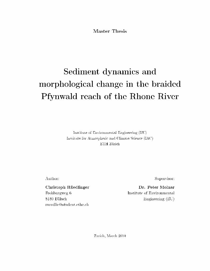
Master Thesis
Sediment dynamics and
morphological change in the braided
Pfynwald reach of the Rhone River
Institute of Environmental Engineering (IfU)
Institute for Atmospheric and Climate Science (IAC)
ETH Zürich
Author:
Christoph Rüedlinger
Frohburgweg 6
8180 Bülach
Supervisor:
Dr. Peter Molnar
Institute of Environmental
Engineering (IfU)
Zurich, March 2010

Abstract
Steep gravel-bed rivers with high sediment supply and stream�ow form a braided channel
structure. The Pfynwald Rhone River reach between Susten and Sierre, located in the
Rhone valley in the Central Alps of Switzerland, has kept its natural braided morphology.
The nearby located Illgraben catchment, which is one of the most active torrents in the
Alps, has a large impact on the characteristics of the Pfynwald River section. There is
large and instantaneous sediment supply to the Rhone River from the Illgraben through
debris �ows. The underlying research hypothesis of this study is that the interactions
of �ow regime, sediment supply and channel morphology are fundamental in order to
quantify the sediment dynamics in braided rivers.
In this thesis the quanti�cation of sediment transport is addressed by means of a
numerical sediment transport model. The one dimensional as well as the two dimensional
model of the numerical sediment transport model system BASEMENT are applied to
the study reach. In the calibration process sensitive model parameters are identi�ed.
The one dimensional model BASEchain is calibrated on the basis of annually sur-
veyed topographic data for the period of 1995 to 2007. The adjusted 10 grain class
model con�guration is then used to investigate the sensitivity of the evolution of the
longitudinal pro�le and of the mean annual sediment transport rate through the reach
with respect to variable boundary conditions.
The two dimensional model BASEplane is calibrated just hydraulically due to a lack
of data for a calibration of sediment transport. The spatial patterns of erosion and
deposition in the channel bed for two di�erent scenarios are addressed with the aid of
the calibrated 2d-model using a mobile riverbed.
On the basis of a balance of observed and computed sediment volumes in the Pfyn-
wald reach the mean annual sediment supply by the Illgraben and the mean annual bed
load transport rate are estimated. For the period of 1995 to 2007 a sediment input of
roughly 140'000m3/a results. The sediment transport rate in the Pfynwald reach de-
creases from 150'000m3/a at the con�uence with the Illgraben to 30'000m3/a at Sierre.
This study highlights that the application of numerical models to relatively steep
alpine rivers with a braided morphology is a very di�cult task and that current nu-
I

II
merical models are not yet fully adequate to simulate satisfactorily sediment transport
and erosion and deposition in such very dynamic river reaches. While the pure hy-
draulic simulations yield excellent results, the sediment transport computations need to
be regarded with extra care, particularly concerning the one dimensional model, which
appeared to su�er from many inconsistencies.

Acknowledgements
I would like to thank all the people who have supported me during the work of my
master thesis. The software I was working with was totally new for me and I was
very glad to have so many competent people around me. I really appreciated their
help and contribution. Special thanks to my supervisor Dr. Peter Molnar for o�ering
this interesting master thesis topic, for his great supervision, for the time he spent for
my concerns and for the many interesting discussions we had. Further I like to thank
the applied numerics divison at the VAW under the direction of Dr. Roland Fäh for
their great e�ort they have brought up to solve the problems I have encountered. A
special thank is dedicated to Renata Müller and Christian Volz for their patience and
for ful�lling my numerous software wishes. Without their help I would not have been
able to manage the modeling part of this thesis. I also like to thank Roni Hunziker
from the engineering company Hunziker, Zarn & Partner AG and Xavier Mittaz from
the engineering company sd ingénierie Dénériaz et Pralong Sion SA who provided me
with several technical reports about the Pfynwald river reach and the topographical
and volumetric data for the calibration of the model. Apart from the above mentioned
people, I would like to thank my family and friends outside ETH who have supported
and encouraged me in numerous ways during my studies.
III

IV
Table of Contents
Abstract I
Acknowledgements III
Table of Contents V
List of Figures IX
List of Tables XI
List of Abbreviations XIII
1 Introduction 1
1.1 Motivation . . . . . . . . . . . . . . . . . . . . . . . . . . . . . . . . . . . 1
1.2 Objectives . . . . . . . . . . . . . . . . . . . . . . . . . . . . . . . . . . . 2
2 Study site 5
2.1 Geographical setting . . . . . . . . . . . . . . . . . . . . . . . . . . . . . 5
2.2 Rhone River . . . . . . . . . . . . . . . . . . . . . . . . . . . . . . . . . . 6
2.2.1 Hydrology . . . . . . . . . . . . . . . . . . . . . . . . . . . . . . . 6
2.2.2 Morphology . . . . . . . . . . . . . . . . . . . . . . . . . . . . . . 9
2.2.3 Topography . . . . . . . . . . . . . . . . . . . . . . . . . . . . . . 10
2.2.4 Sediment grain size distribution . . . . . . . . . . . . . . . . . . . 11
2.2.5 Gravel extraction . . . . . . . . . . . . . . . . . . . . . . . . . . . 12
2.3 Illgraben . . . . . . . . . . . . . . . . . . . . . . . . . . . . . . . . . . . . 13
2.3.1 General description . . . . . . . . . . . . . . . . . . . . . . . . . . 13
2.3.2 Sediment grain size distribution . . . . . . . . . . . . . . . . . . . 13
2.3.3 Observation . . . . . . . . . . . . . . . . . . . . . . . . . . . . . . 14
3 Numerical sediment transport model 17
3.1 Introduction . . . . . . . . . . . . . . . . . . . . . . . . . . . . . . . . . . 17
V
VI
3.1.1 Mathematical-physical modules . . . . . . . . . . . . . . . . . . . 18
3.1.2 Computational grid . . . . . . . . . . . . . . . . . . . . . . . . . . 19
3.1.3 Numerical modules . . . . . . . . . . . . . . . . . . . . . . . . . . 20
3.2 Goals . . . . . . . . . . . . . . . . . . . . . . . . . . . . . . . . . . . . . 20
3.2.1 1d-model BASEchain . . . . . . . . . . . . . . . . . . . . . . . . . 20
3.2.2 2d-model BASEplane . . . . . . . . . . . . . . . . . . . . . . . . . 20
3.3 Preprocessing . . . . . . . . . . . . . . . . . . . . . . . . . . . . . . . . . 21
3.3.1 Project BASEchain (1D) . . . . . . . . . . . . . . . . . . . . . . . 22
3.3.2 Project BASEplane (2D) . . . . . . . . . . . . . . . . . . . . . . . 24
4 Model calibration 27
4.1 Project BASEchain (1D) . . . . . . . . . . . . . . . . . . . . . . . . . . . 27
4.1.1 Input data . . . . . . . . . . . . . . . . . . . . . . . . . . . . . . . 28
4.1.2 Calibration parameters . . . . . . . . . . . . . . . . . . . . . . . . 29
4.1.3 Calibration results . . . . . . . . . . . . . . . . . . . . . . . . . . 33
4.1.4 Best �t . . . . . . . . . . . . . . . . . . . . . . . . . . . . . . . . 41
4.2 Project BASEplane (2D) . . . . . . . . . . . . . . . . . . . . . . . . . . . 44
4.2.1 Input data . . . . . . . . . . . . . . . . . . . . . . . . . . . . . . . 44
4.2.2 Calibration parameters . . . . . . . . . . . . . . . . . . . . . . . . 44
4.2.3 Calibration results . . . . . . . . . . . . . . . . . . . . . . . . . . 45
5 Scenario analysis 51
5.1 Project BASEchain (1D) . . . . . . . . . . . . . . . . . . . . . . . . . . . 51
5.1.1 Sensitivity to sediment extraction . . . . . . . . . . . . . . . . . . 52
5.1.2 Sensitivity to sediment supply by the Illgraben . . . . . . . . . . 53
5.2 Project BASEplane (2D) . . . . . . . . . . . . . . . . . . . . . . . . . . . 54
5.2.1 Simulation of the sediment in�ow at the upper boundary condition 55
5.2.2 Simulation of a debris �ow event . . . . . . . . . . . . . . . . . . 56
6 Discussion 59
6.1 Project BASEchain (1D) . . . . . . . . . . . . . . . . . . . . . . . . . . . 59
6.1.1 Model calibration . . . . . . . . . . . . . . . . . . . . . . . . . . . 59
6.1.2 Scenario analysis . . . . . . . . . . . . . . . . . . . . . . . . . . . 65
6.1.3 Limitations of the model . . . . . . . . . . . . . . . . . . . . . . . 67
6.2 Project BASEplane (2D) . . . . . . . . . . . . . . . . . . . . . . . . . . . 68
6.2.1 Model calibration . . . . . . . . . . . . . . . . . . . . . . . . . . . 68
6.2.2 Scenario analysis . . . . . . . . . . . . . . . . . . . . . . . . . . . 70
Table of Contents VII
7 Conclusion and outlook 73
7.1 Conclusion . . . . . . . . . . . . . . . . . . . . . . . . . . . . . . . . . . . 73
7.2 Outlook . . . . . . . . . . . . . . . . . . . . . . . . . . . . . . . . . . . . 75
References 79
Appendix 81
A Observation of debris �ows in the Illgraben . . . . . . . . . . . . . . . . 81
B ROC plots and accuracy statistic T . . . . . . . . . . . . . . . . . . . . . 83

VIII
List of Figures
2.1 Overview of the Pfynwald reach of the Rhone River . . . . . . . . . . . . 5
2.2 Reconstructed mean monthly discharge in the Pfynwald reach . . . . . . 7
2.3 Flood frequency analysis for the Pfynwald reach . . . . . . . . . . . . . . 8
2.4 Braided morphology in the Pfynwald river reach . . . . . . . . . . . . . . 9
2.5 Evolution of the longitudinal pro�le in the period of 1995 to 2007 . . . . 10
2.6 Observed characteristic grain sizes dm and d90 in the Rhone . . . . . . . 11
2.7 Grain size distribution of one particular debris �ow . . . . . . . . . . . . 14
2.8 Visual impression of the debris �ow material . . . . . . . . . . . . . . . . 15
2.9 Con�uence of the Illgraben and the Rhone River . . . . . . . . . . . . . 15
3.1 Modules of BASEMENT . . . . . . . . . . . . . . . . . . . . . . . . . . . 18
3.2 Overview of the di�erent project domains . . . . . . . . . . . . . . . . . 21
3.3 Mesh of the study area for the 2d modeling . . . . . . . . . . . . . . . . 25
4.1 Observed and simulated characteristic grain sizes dm and d90 . . . . . . 32
4.2 Result of the hydraulic simulation . . . . . . . . . . . . . . . . . . . . . . 33
4.3 Simulation results using di�erent values for the calibration parameter
upwind . . . . . . . . . . . . . . . . . . . . . . . . . . . . . . . . . . . . . 35
4.4 Simulation results using di�erent active layer heights . . . . . . . . . . . 36
4.5 Calibration results of single grain simulations . . . . . . . . . . . . . . . 37
4.6 Simulation results using di�erent numbers of grain classes . . . . . . . . 39
4.7 Simulation results using di�erent compositions of the debris �ow material 40
4.8 Simulation results of the model con�guration that �ts the observations best 42
4.9 Temporal evolution of the mean riverbed elevation in the period 1995 to
2007. . . . . . . . . . . . . . . . . . . . . . . . . . . . . . . . . . . . . . . 43
4.10 Subdivision of the 2D model domain . . . . . . . . . . . . . . . . . . . . 45
4.11 Receiver-operation characteristics (ROC) plot . . . . . . . . . . . . . . . 47
4.12 Accuracy statistic T . . . . . . . . . . . . . . . . . . . . . . . . . . . . . 48
4.13 Best �t of the 2D model . . . . . . . . . . . . . . . . . . . . . . . . . . . 49
IX
X
5.1 Result of the scenario concerning no gravel extraction . . . . . . . . . . 52
5.2 Result of the scenario modeling di�erent supplies by the Illgraben . . . . 54
5.3 Simulated riverbed changes with a sediment �ux at the upper boundary 56
5.4 Computed riverbed changes for the scenario describing a debris �ow sim-
ulation . . . . . . . . . . . . . . . . . . . . . . . . . . . . . . . . . . . . . 57
5.5 Simulated water depth and velocity vectors for the scenario describing a
debris �ow simulation . . . . . . . . . . . . . . . . . . . . . . . . . . . . 58
6.1 Results of the sediment relocation test . . . . . . . . . . . . . . . . . . . 63
B.1 Receiver-operation characteristics (ROC) plot and accuracy statistic T . 83
List of Tables
2.1 Expected �ood peaks in the Pfynwald reach . . . . . . . . . . . . . . . . 8
2.2 Gravel extraction volumes in the Pfynwald river section . . . . . . . . . 12
4.1 Sediment balance in the Pfynwald reach . . . . . . . . . . . . . . . . . . 29
4.2 Confusion matrix (or contingency table) . . . . . . . . . . . . . . . . . . 46
4.3 Calibrated and computed roughness coe�cients . . . . . . . . . . . . . . 47
5.1 Overview of the investigated scenarios with BASEchain . . . . . . . . . 51
5.2 Overview of the investigated scenarios with BASEplane . . . . . . . . . 55
A.1 Sediment volumes of observed debris �ow events in the Illgraben in the
period of 2000 to 2005 . . . . . . . . . . . . . . . . . . . . . . . . . . . . 81
A.2 Sediment volumes of observed debris �ow events in the Illgraben in the
period of 1932 to 1999 . . . . . . . . . . . . . . . . . . . . . . . . . . . . 82
XI

XII
List of Abbreviations
BASEMENT . BASic EnvironMENT for simulation of environmental �ow and natural
hazard simulation
CFL . . . . . . . . . Courant-Friedrichs-Lewy
CS . . . . . . . . . . . Cross Section
DEM . . . . . . . . Digital Elevation Model
DTM-AV . . . . Digitales Terrainmodell der Amtlichen Vermessung
ETH . . . . . . . . . Swiss Federal Institute of Technology
FV . . . . . . . . . . . Finite Volume
HLL . . . . . . . . . Harten, Lax, van Leer
HLLC . . . . . . . . Harten-Lax-van Leer-Contact
IVP . . . . . . . . . . Initial Value Problem
LIDAR . . . . . . Light Detection And Ranging
MPM . . . . . . . . Meyer-Peter Müller (sediment transport formula)
MPMH . . . . . . Meyer-Peter Müller Hunziker (sediment transport formula)
RECORD . . . . Restored Corridor Dynamics
ROC . . . . . . . . . Receiver-Operation Characteristics
SMS . . . . . . . . . Surface Water Modeling System
VAW . . . . . . . . . Laboratory of Hydraulics, Hydrology and Glaciology
XIII

XIV
Chapter 1
Introduction
1.1 Motivation
Natural rivers show a large variety of channel patterns. Leopold and Wolman (1957)
developed a widely used classi�cation scheme for natural rivers based on their planform.
They suggest a division of the morphology of a river channel into the three categories:
straight, meandering and braided. In a natural environment rivers develop generally
from a straight to a braided channel structure with increasing slope and coarser gravel.
Among straight, meandering and braided rivers, the latter are the most dynamic
systems. Short-term channel migration is a frequently seen phenomenon in braided
rivers, because steep headwater tributaries supply highly variable discharges and sedi-
ment supply to the mainstream (Gray and Hardling , 2007). A simple and commonly
used de�nition from Leopold and Wolman (1957) describes braided river morphology
as a river, which �ows in two or more anastomosing channels around alluvial islands.
Braided rivers can be found all over the world, most frequently they occur in Arctic and
Alpine regions that are characterized by high precipitation and steep headwaters (Gray
and Hardling , 2007).
Braided river morphology is determined to a large extent by the dynamics in gravel-
size sediment availability, supply and transport. It is most widespread in gravel-bed
rivers where the coarse grains are close to incipient motion conditions during large and
relatively frequent discharges, so that the river is subject to permanent changes in the
channel bed structure.
In the course of large-scale river corrections in the last two centuries, most Alpine
rivers were straightened and channelized. The original meandering and braided river
systems disappeared almost completely in Central Europe. The Pfynwald reach of the
Rhone River between Susten and Sierre is one of the last morphologically intact braided
river section in Switzerland that kept its original dynamics. The natural dynamics of the
1
2
river has so far not allowed to channelize this section of the Rhone River. The Pfynwald
reach of the Rhone River is therefore a very unique place to study extremely active river
dynamics and the relevant consequences to river management.
The natural dynamics of the Pfynwald Rhone River section is mainly caused by the
large sediment supply by the Illgraben, a tributary that joins the Rhone River near
Susten. The Illgraben catchment is one of the most active torrents in the Alps. Every
year several thousand tons of sediment are delivered to the Rhone River by debris �ows
(Hürlimann et al., 2003).
Sediment discharge from a tributary to a main valley can in�uence the �ow pattern
of the receiving trunk stream, if the increase in sediment �ux exceeds the sediment
transport capacity of the river. Studies conducted in other rivers show that an imbalance
between stream power and sediment transport capacity occurs at the con�uence of two
streams with contrasting hydrological properties (Hammack and Wohl , 1996; Tucker and
Slingerland , 1997; Korup, 2004; Hanks and Webb, 2006).
Investigations of Jäggi (1988) and Bezzola (1989) show that there is an imbalance
between stream power and sediment transport capacity in the Pfynwald reach of the
Rhone River. In particular, the large and instantaneous sediment inputs from the Ill-
graben especially lead to aggradation in the channel bed of the Rhone River. Since
the year 1995 annual sediment volume balances of the Pfynwald river reach have been
estimated by a local engineering company (KBM SA, 1995-2007). In addition the sed-
iment balance as well as the morphology of the respective reach was investigated with
the aid of a numerical model (Hunziker, Zarn & Partner AG , 2001). The applied one
dimensional sediment transport model su�ered from numerical instabilities due to the
frequent hydraulic drops in this relatively steep river reach.
Since humans impact the Rhone River system through �ow regulation and gravel
extraction, it is of great importance to understand and to quantify the sediment dy-
namics in the natural Pfynwald River reach, not only with respect to the ongoing river
restoration project of the third Rhone River correction, but also to contribute to the
scienti�c understanding of �uvial processes in gravel-bed braided rivers in general.
1.2 Objectives
The goal of this Master Thesis is to model sediment transport in the braided Pfynwald
section of the Rhone River by means of the software system BASEMENT. Both the one
dimensional as well as the two dimensional sediment transport model of BASEMENT
are applied to the investigated river reach. A special focus is set to the response of
the riverbed of the Rhone to massive sediment inputs through debris �ows from the
Illgraben. The underlying hypothesis is that understanding the interactions of �ow

Introduction 3
regime, sediment supply and channel morphology is fundamental for quantifying the
sediment dynamics in steep gravel-bed rivers. Within the described framework the
following �ve objectives are addressed in this thesis:
1. Computation of a sediment balance for the Pfynwald river reach in order to es-
timate the mean annual sediment supply by the Illgraben and to quantify the
observed mean annual sediment transport rate through the study reach
2. Reproduction of the observed mean annual sediment transport rate by means of a
one dimensional numerical sediment transport model
3. Identi�cation of sensitive model parameters with respect to the model output
4. Analysis of the sensitivity of the Pfynwald river reach to variable boundary con-
ditions
5. Investigation of spatial patterns of sedimentation and erosion at the con�uence
of the Rhone River and the Illgraben with a two dimensional sediment transport
model

4
Chapter 2
Study site
2.1 Geographical setting
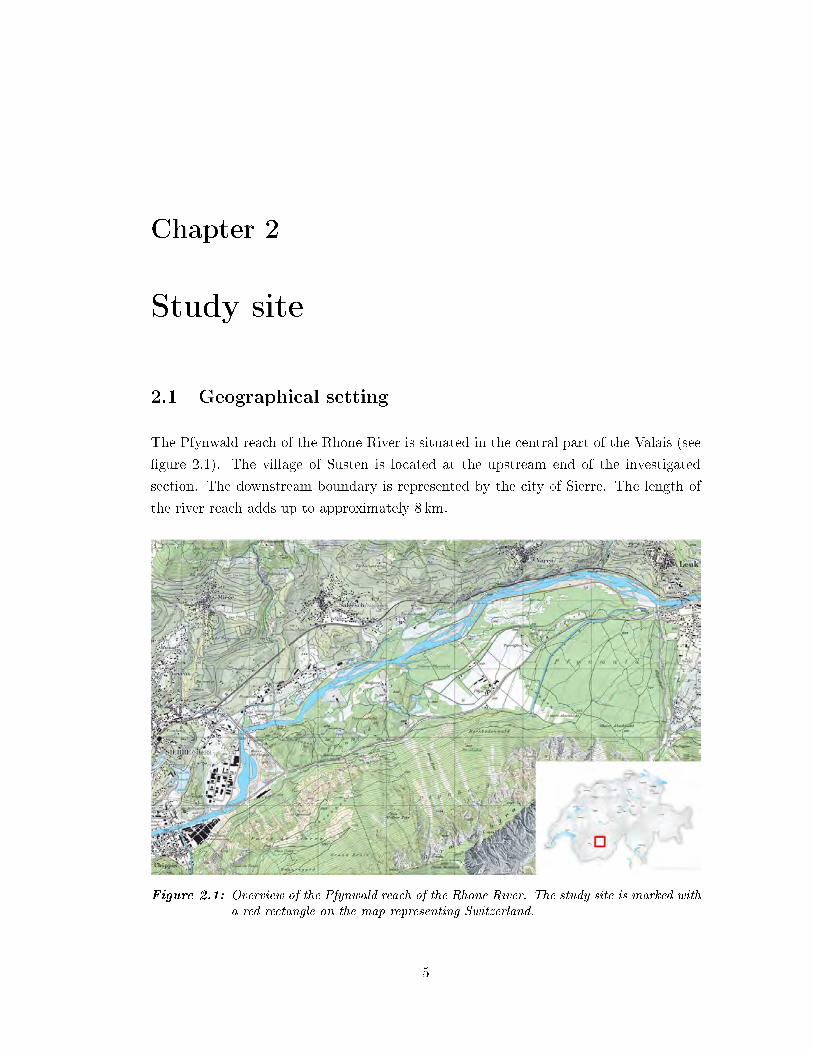
The Pfynwald reach of the Rhone River is situated in the central part of the Valais (see
�gure 2.1). The village of Susten is located at the upstream end of the investigated
section. The downstream boundary is represented by the city of Sierre. The length of
the river reach adds up to approximately 8 km.
Figure 2.1: Overview of the Pfynwald reach of the Rhone River. The study site is marked witha red rectangle on the map representing Switzerland.
5
6
2.2 Rhone River
The Rhone is one of the major rivers in Europe, draining large areas of the north-western
Alps and the Jura mountains. The river rises as the e�uent of the Rhone Glacier in the
central Swiss Alps. On its 812 km long way to the Mediterranean Sea it �rst drains the
Valais and several tributary valleys before entering Lake Geneva. On its further route
the Rhone runs through south-eastern France and enters the Mediterranean Sea close
to the city of Arles.
2.2.1 Hydrology
The hydrological regime of the Rhone cannot be allocated to one speci�c regime type. In
fact it is a combination of glacial, nival and pluvial regime with low �ows in wintertime
and high �ows during summertime. The initiation of the large reservoir power stations
Grande Dixcence (1956), Mauvoisin (1957), Mattmark (1967) and Emosson (1974) in
the catchment area of the Rhone River caused a signi�cant change of the stream�ow
regime. The mentioned reservoirs retain the large melt water discharge in spring and
summer and release it during low �ow periods in winter. Consequently natural �oods
are reduced and discharge during low �ow season is increased.
Particularly in the Pfynwald section of the Rhone River the �ow regime is signif-
icantly in�uenced by a weir situated at the village of Susten. Since the year 1911,
when the barrage was brought into service, up to 65m3/s of water are extracted and
delivered to a power plant at Chippis through a separate channel. Before autumn 2008
the riverbed underneath the weir used to stay dry, if discharge at Susten went below
the maximum extraction volume of 65m3/s. In the course of the renewal of the power
plants concession, the operating company is bounded to guarantee a residual discharge
of 3,25m3/s in the Pfynwald reach of the Rhone River from that time on.
There is no gauging station located directly on the river reach between Susten and
Sierre. Discharge measurements are taken either in Brig, located 30 km upstream, or
in Sion that lies 25 km downstream of Susten. Stream�ow data at the top end of the
Pfynwald reach is therefore reconstructed from the hydrometric gauging stations in Brig
and Sion. The correlation between the size of the catchment and the measured discharge
was used to set up a relationship that allows computing discharge in the Pfynwald reach.
QPfynwald = QBrig + a · (QSion −QBrig)− 60m3/s
with a = 0.6
The factor a was calculated based on the di�erences between catchment sizes at Brig
Study site 7
1 2 3 4 5 6 7 8 9 10 11 120
20
40
60
80
100
120
140
160
180
200
month
dis
ch
arg
e [m
3/s
]
discharge Susten
discharge Pfynwald
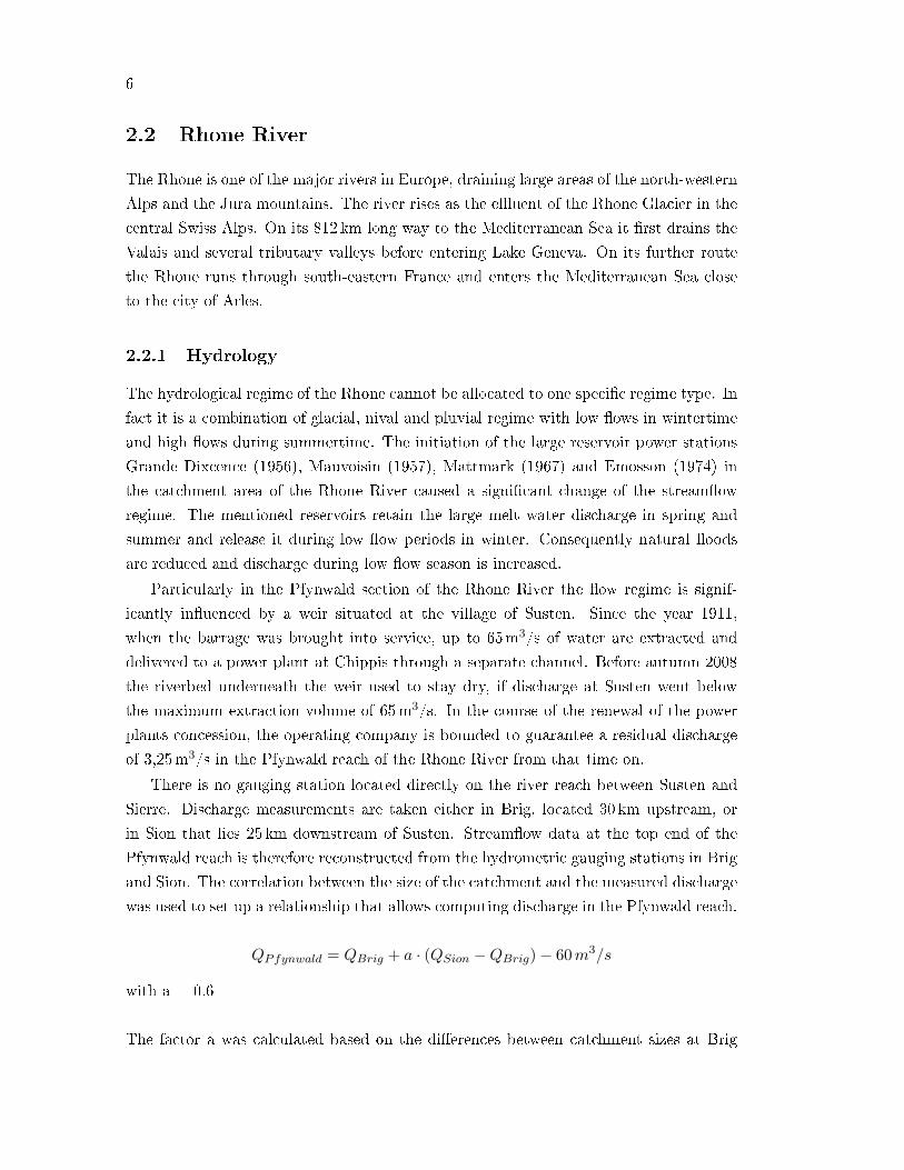
Figure 2.2: Reconstructed mean monthly discharge in the Pfynwald reach of the Rhone Riverbased on observed stream�ow at measuring gauges at Brig and Sion.
(913 km3), Susten (2400 km3) and Sion (3373 km3). The underlying assumption states
that discharge increases with growing catchment size. Additionally the water extraction
at the weir at Susten has to be considered, since this signi�cantly changes stream�ow
conditions downstream of the weir. The determined discharge, based on the observations
at Brig and Visp, was therefore reduced by a constant extraction volume of 60m3/s. Fig-
ure 2.2 shows the mean monthly discharge for the period of 1974 to 2008. One can see
that there is no discharge during low �ow periods due to the water extraction at the
weir in Susten.
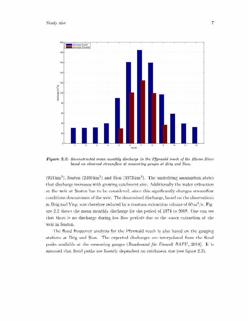
The �ood frequency analysis for the Pfynwald reach is also based on the gauging
stations at Brig and Sion. The expected discharges are interpolated from the �ood
peaks available at the measuring gauges (Bundesamt für Umwelt BAFU , 2010). It is
assumed that �ood peaks are linearly dependent on catchment size (see �gure 2.3).
8
500 1000 1500 2000 2500 3000 3500200
300
400
500
600
700
800
900
1000
1100
catchment area [km3]
dis
ch
arg
e [m
3/s
]
R=2R=5R=10R=30R=50R=100R=300
SionPfynwaldBrig
Figure 2.3: Interpolation of �oods with return periods of 2, 5, 10, 20, 50, 100 and 300 years inthe Pfynwald reach based on the �ood frequency analysis at the measuring gaugesBrig and Sion.
Table 2.1: Expected �ood peaks in thePfynwald reach
return period discharge
Susten Pfynwald
2 376 316
5 467 407
10 532 532
30 636 636
50 686 686
100 757 757
300 878 878
The resulting �ood peaks for the Pfynwald
reach of the Rhone River are summarized in
table 2.1. In case of extreme �oods (August
1987, September 1993, October 2000) the weir
at Susten is not anymore in use (Hunziker,
Zarn & Partner AG , 2001). Thus discharge is
�owing completely through the Pfynwald reach
and the extraction volume has not to be con-
sidered. The critical discharge at which the
water extraction is stopped is not known. For
this study it is assumed to correspond to a dis-
charge with a return period of 10 years.
Study site 9
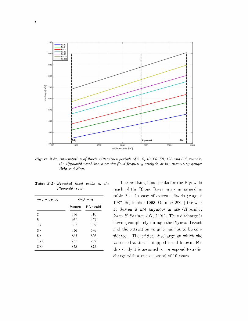
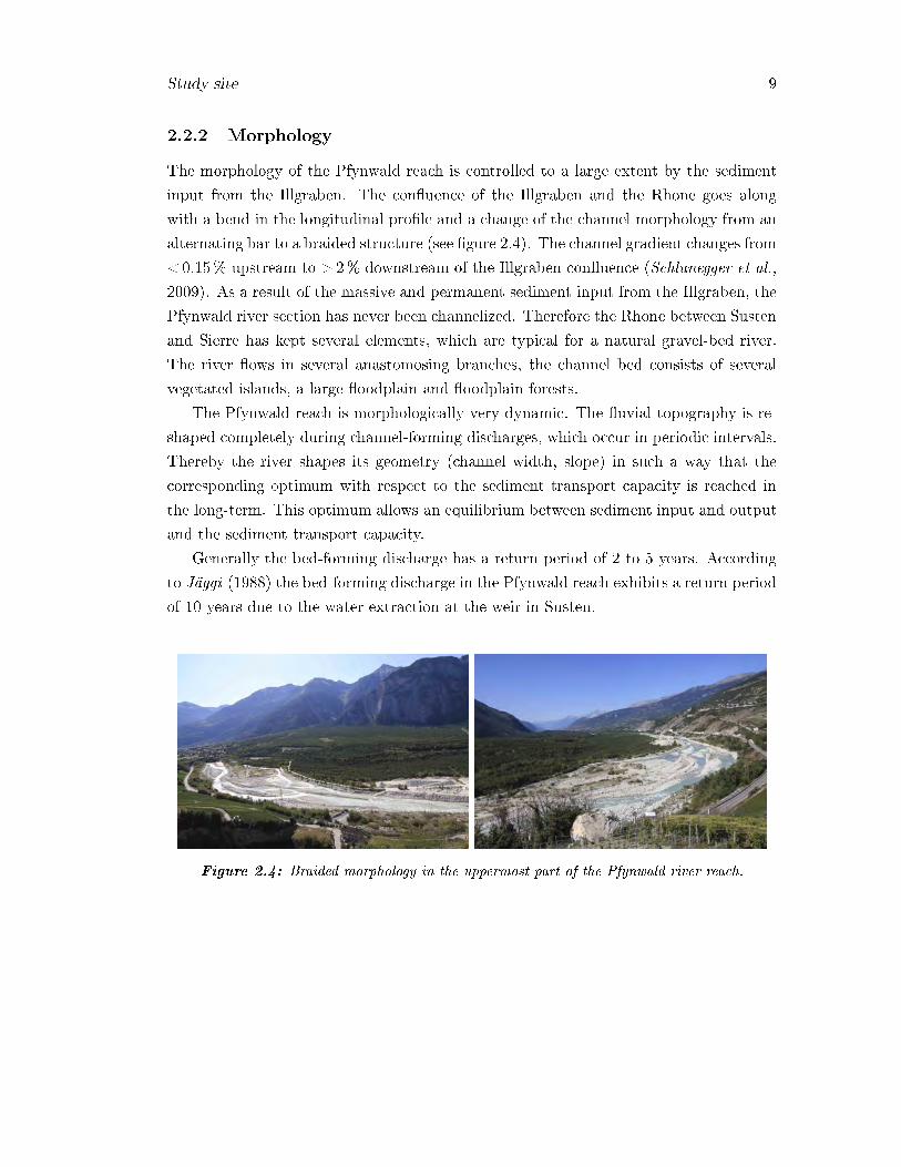
2.2.2 Morphology
The morphology of the Pfynwald reach is controlled to a large extent by the sediment
input from the Illgraben. The con�uence of the Illgraben and the Rhone goes along
with a bend in the longitudinal pro�le and a change of the channel morphology from an
alternating bar to a braided structure (see �gure 2.4). The channel gradient changes from
<0.15% upstream to >2% downstream of the Illgraben con�uence (Schlunegger et al.,
2009). As a result of the massive and permanent sediment input from the Illgraben, the
Pfynwald river section has never been channelized. Therefore the Rhone between Susten
and Sierre has kept several elements, which are typical for a natural gravel-bed river.
The river �ows in several anastomosing branches, the channel bed consists of several
vegetated islands, a large �oodplain and �oodplain forests.
The Pfynwald reach is morphologically very dynamic. The �uvial topography is re-
shaped completely during channel-forming discharges, which occur in periodic intervals.
Thereby the river shapes its geometry (channel width, slope) in such a way that the
corresponding optimum with respect to the sediment transport capacity is reached in
the long-term. This optimum allows an equilibrium between sediment input and output
and the sediment transport capacity.
Generally the bed-forming discharge has a return period of 2 to 5 years. According
to Jäggi (1988) the bed-forming discharge in the Pfynwald reach exhibits a return period
of 10 years due to the water extraction at the weir in Susten.
Figure 2.4: Braided morphology in the uppermost part of the Pfynwald river reach.
10
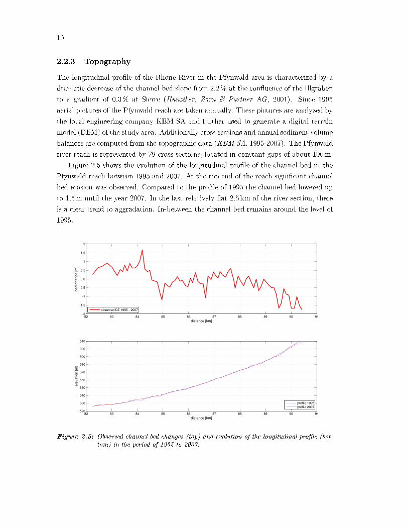
2.2.3 Topography
The longitudinal pro�le of the Rhone River in the Pfynwald area is characterized by a
dramatic decrease of the channel bed slope from 2.2% at the con�uence of the Illgraben
to a gradient of 0.3% at Sierre (Hunziker, Zarn & Partner AG , 2001). Since 1995
aerial pictures of the Pfynwald reach are taken annually. These pictures are analyzed by
the local engineering company KBM SA and further used to generate a digital terrain
model (DEM) of the study area. Additionally cross sections and annual sediment volume
balances are computed from the topographic data (KBM SA, 1995-2007). The Pfynwald
river reach is represented by 79 cross sections, located in constant gaps of about 100m.
Figure 2.5 shows the evolution of the longitudinal pro�le of the channel bed in the
Pfynwald reach between 1995 and 2007. At the top end of the reach signi�cant channel
bed erosion was observed. Compared to the pro�le of 1995 the channel bed lowered up
to 1.5m until the year 2007. In the last relatively �at 2.5 km of the river section, there
is a clear trend to aggradation. In-between the channel bed remains around the level of
1995.
82 83 84 85 86 87 88 89 90 91-2
-1.5
-1
-0.5
0
0.5
1
1.5
2
distance [km]
be
d c
ha
ng
e [m
]
observed DZ 1995 - 2007
82 83 84 85 86 87 88 89 90 91520
530
540
550
560
570
580
590
600
610
distance [km]
ele
va
tio
n [m
]
profile 1995
profile 2007
Figure 2.5: Observed channel bed changes (top) and evolution of the longitudinal pro�le (bot-tom) in the period of 1995 to 2007.
Study site 11
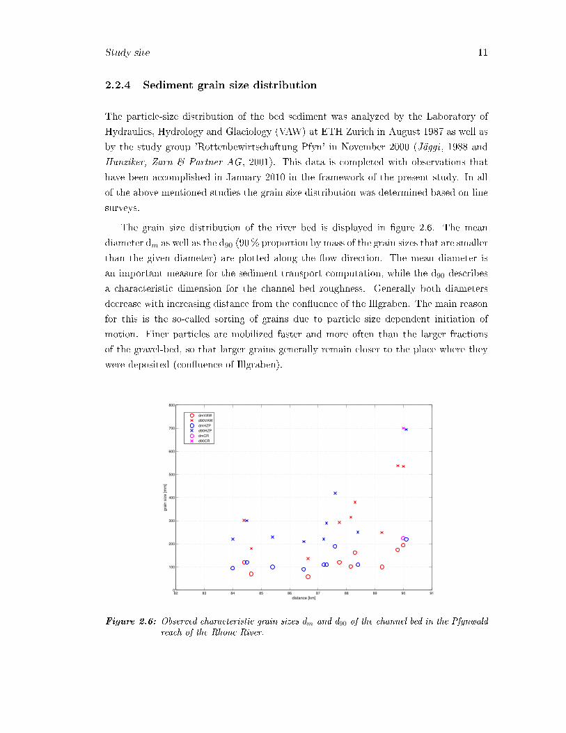
2.2.4 Sediment grain size distribution
The particle-size distribution of the bed sediment was analyzed by the Laboratory of
Hydraulics, Hydrology and Glaciology (VAW) at ETH Zurich in August 1987 as well as
by the study group 'Rottenbewirtschaftung Pfyn' in November 2000 (Jäggi , 1988 and
Hunziker, Zarn & Partner AG , 2001). This data is completed with observations that
have been accomplished in January 2010 in the framework of the present study. In all
of the above mentioned studies the grain size distribution was determined based on line
surveys.
The grain size distribution of the river bed is displayed in �gure 2.6. The mean
diameter dm as well as the d90 (90% proportion by mass of the grain sizes that are smaller
than the given diameter) are plotted along the �ow direction. The mean diameter is
an important measure for the sediment transport computation, while the d90 describes
a characteristic dimension for the channel bed roughness. Generally both diameters
decrease with increasing distance from the con�uence of the Illgraben. The main reason
for this is the so-called sorting of grains due to particle size dependent initiation of
motion. Finer particles are mobilized faster and more often than the larger fractions
of the gravel-bed, so that larger grains generally remain closer to the place where they
were deposited (con�uence of Illgraben).
82 83 84 85 86 87 88 89 90 910
100
200
300
400
500
600
700
800
distance [km]
gra
in s
ize
[m
m]
dmVAW
d90VAW
dmHZP
d90HZP
dmCR
d90CR
Figure 2.6: Observed characteristic grain sizes dm and d90 of the channel bed in the Pfynwaldreach of the Rhone River.
12
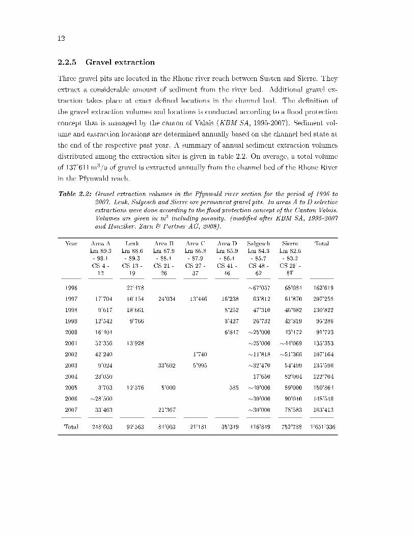
2.2.5 Gravel extraction
Three gravel pits are located in the Rhone river reach between Susten and Sierre. They
extract a considerable amount of sediment from the river bed. Additional gravel ex-
traction takes place at exact de�ned locations in the channel bed. The de�nition of
the gravel-extraction volumes and locations is conducted according to a �ood protection
concept that is managed by the canton of Valais (KBM SA, 1995-2007). Sediment vol-
ume and extraction locations are determined annually based on the channel bed state at
the end of the respective past year. A summary of annual sediment extraction volumes
distributed among the extraction sites is given in table 2.2. On average, a total volume
of 137'611m3/a of gravel is extracted annually from the channel bed of the Rhone River
in the Pfynwald reach.
Table 2.2: Gravel extraction volumes in the Pfynwald river section for the period of 1996 to2007. Leuk, Salgesch and Sierre are permanent gravel pits. In areas A to D selectiveextractions were done according to the �ood protection concept of the Canton Valais.Volumes are given in m3 including porosity. (modi�ed after KBM SA, 1995-2007and Hunziker, Zarn & Partner AG, 2008).
Year Area A Leuk Area B Area C Area D Salgesch Sierre Totalkm 89.3- 90.1
km 88.6- 89.3
km 87.9- 88.4
km 86.8- 87.9
km 85.9- 86.4
km 84.3- 85.7
km 82.6- 83.2
CS 4 -12
CS 13 -19
CS 21 -26
CS 27 -37
CS 41 -46
CS 48 -62
CS 2F -8F
1996 27'478 ∼67'057 68'084 162'619
1997 17'704 10'154 24'034 13'446 16'238 63'812 61'870 207'258
1998 9'617 18'661 8'252 47'310 46'982 130'822
1999 12'542 9'766 3'427 26'732 42'819 95'286
2000 16'404 6'847 ∼25'000 43'472 91'723
2001 52'356 13'928 ∼25'000 ∼44'069 135'353
2002 42'240 1'740 ∼11'818 ∼51'366 107'164
2003 9'024 33'602 5'995 ∼32'470 54'499 135'590
2004 23'050 17'650 82'004 122'704
2005 3'703 12'576 5'000 585 ∼40'000 89'000 150'864
2006 ∼28'500 ∼30'000 90'040 148'540
2007 33'463 21'367 ∼30'000 78'583 163'413
Total 248'603 92'563 84'003 21'181 35'349 416'849 752'788 1'651'336
Study site 13
2.3 Illgraben
2.3.1 General description
The Illgraben catchment is one of the most active torrents in the Alps. Every year several
thousand tons of sediment are delivered to the Rhone River by debris �ows (Hürlimann
et al., 2003). Since the last Ice Age a more than 100m-thick fan of gravel covering an
area of 6.6 km2 has formed in the Rhone Valley. The Rhone River is therefore de�ected
to the north side of the valley. The Illgraben merges the Rhone River at their left bank
roughly 500m meters downstream of the weir at Susten. The catchment area of the
torrent is about 10 km2. Geologically the Illgraben catchment lies in Triassic schists and
dolobreccias. The matrix of the debris �ow material is silt, clay and quartzites, which
are prone to erosion during heavy rainfall events (e.g. summer thunderstorms). Average
erosion rates are as high as 7 cm per year (Hürlimann et al., 2003 and McArdell et al.,
2007).
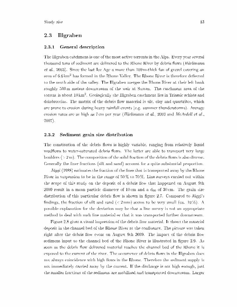
2.3.2 Sediment grain size distribution
The constitution of the debris �ows is highly variable, ranging from relatively liquid
mud�ows to water-saturated debris �ows. The latter are able to transport very large
boulders (> 2m). The composition of the solid fraction of the debris �ows is also diverse.
Generally the �ner fractions (silt and sand) account for a quite substantial proportion.
Jäggi (1988) estimates the fraction of the �nes that is transported away by the Rhone
River in suspension to be in the range of 50% to 70%. Line surveys carried out within
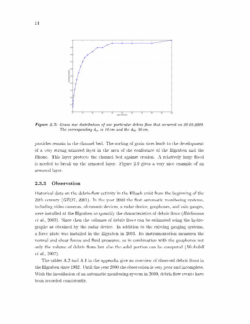
the scope of this study on the deposit of a debris �ow that happened on August 9th
2009 result in a mean particle diameter of 10 cm and a d90 of 30 cm. The grain size
distribution of this particular debris �ow is shown in �gure 2.7. Compared to Jäggi's
�ndings, the fraction of silt and sand (<2mm) seems to be very small (ca. 10%). A
possible explanation for the deviation may be that a line survey is not an appropriate
method to deal with such �ne material or that it was transported further downstream.
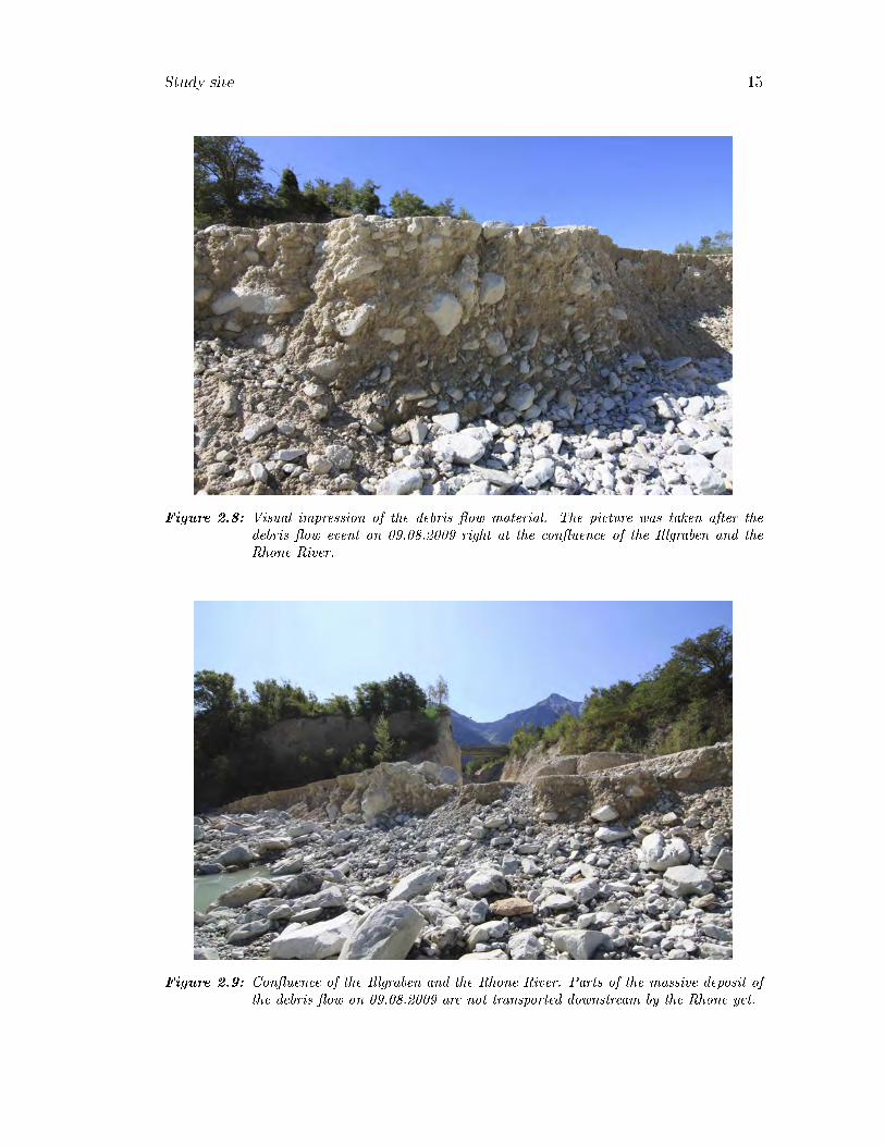
Figure 2.8 gives a visual impression of the debris �ow material. It shows the material
deposit in the channel bed of the Rhone River at the con�uence. The picture was taken
right after the debris �ow event on August 9th 2009. The impact of the debris �ow
sediment input to the channel bed of the Rhone River is illustrated in �gure 2.9. As
soon as the debris �ow delivered material reaches the channel bed of the Rhone it is
exposed to the current of the river. The occurrence of debris �ows in the Illgraben does
not always coincidence with high �ows in the Rhone. Therefore the sediment supply is
not immediately carried away by the current. If the discharge is not high enough, just
the smaller fractions of the sediment are mobilized and transported downstream. Larger
14
0 10 20 30 40 50 60 70 80 90 1000
0.1
0.2
0.3
0.4
0.5
0.6
0.7
0.8
0.9
1
grain size [cm]
cu
mu
lative
fra
ctio
n
Figure 2.7: Grain size distribution of one particular debris �ow that occurred on 09.08.2009.The corresponding dm is 10 cm and the d90 30 cm.
particles remain in the channel bed. The sorting of grain sizes leads to the development
of a very strong armored layer in the area of the con�uence of the Illgraben and the
Rhone. This layer protects the channel bed against erosion. A relatively large �ood
is needed to break up the armored layer. Figure 2.9 gives a very nice example of an
armored layer.
2.3.3 Observation
Historical data on the debris-�ow activity in the Illbach exist from the beginning of the
20th century (GEO7 , 2001). In the year 2000 the �rst automatic monitoring systems,
including video cameras, ultrasonic devices, a radar device, geophones, and rain gauges,
were installed at the Illgraben to quantify the characteristics of debris �ows (Hürlimann
et al., 2003). Since then the volumes of debris �ows can be estimated using the hydro-
graphs as obtained by the radar device. In addition to the existing gauging systems,
a force plate was installed in the Illgraben in 2003. Its instrumentation measures the
normal and shear forces and �uid pressures, so in combination with the geophones not
only the volume of debris �ows but also the solid portion can be computed (McArdell
et al., 2007).
The tables A.2 and A.1 in the appendix give an overview of observed debris �ows in
the Illgraben since 1932. Until the year 2000 the observation is very poor and incomplete.
With the installation of an automatic monitoring system in 2000, debris �ow events have
been recorded consistently.
Study site 15
Figure 2.8: Visual impression of the debris �ow material. The picture was taken after thedebris �ow event on 09.08.2009 right at the con�uence of the Illgraben and theRhone River.
Figure 2.9: Con�uence of the Illgraben and the Rhone River. Parts of the massive deposit ofthe debris �ow on 09.08.2009 are not transported downstream by the Rhone yet.

16
Chapter 3
Numerical sediment transport
model
3.1 Introduction
The numerical sediment transport model system applied in this study is called BASE-
MENT (Faeh et al., 2006-2008). The development of this software started in the year
2002 and is still maintained by the applied numerics division at the Laboratory of Hy-
draulics, Hydrology and Glaciology (VAW). The name BASEMENT stands for BASic
EnvironMENT for simulation of environmental �ow and natural hazard simulation. The
software consists of the numerical solution algorithms, included in di�erent modules.
Pre- and post-processing has to be done with independent products. So far BASE-
MENT consists of two subsystems, a one-dimensional tool called BASEchain and a
two-dimensional module named BASEplane. Both are able to simulate �ow behavior
and sediment transport under steady and unsteady conditions in a channel. In the scope
of this work the currently available version 1.7 of the numerical tools BASEchain and
BASEplane was applied.
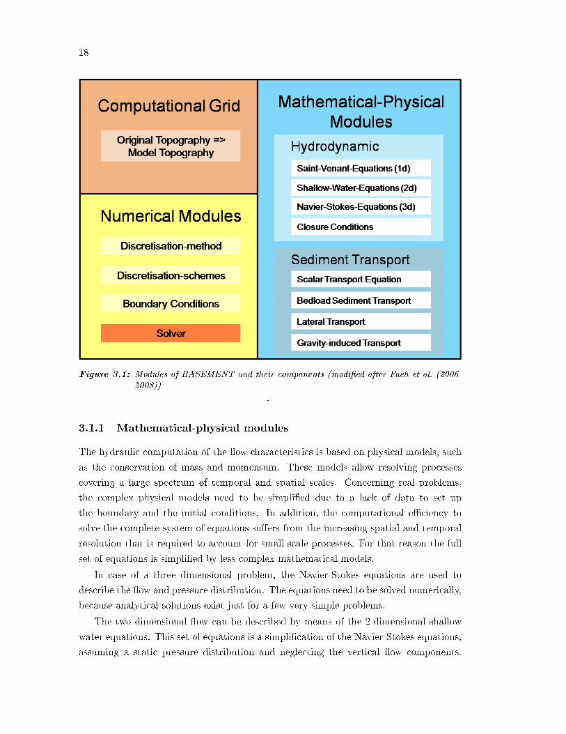
The simulation tools are further partitioned into three di�erent parts (Faeh et al.,
2006-2008):
• the mathematical-physical modules consisting of the governing �ow equations
• the computational grid representing the discrete form of the topography
• the numerical modules with their methods for solving the equations
Figure 3.1 gives a graphical overview of the di�erent modules and their components.
17
18
Figure 3.1: Modules of BASEMENT and their components (modi�ed after Faeh et al. (2006-2008))
.
3.1.1 Mathematical-physical modules
The hydraulic computation of the �ow characteristics is based on physical models, such
as the conservation of mass and momentum. These models allow resolving processes
covering a large spectrum of temporal and spatial scales. Concerning real problems,
the complex physical models need to be simpli�ed due to a lack of data to set up
the boundary and the initial conditions. In addition, the computational e�ciency to
solve the complete system of equations su�ers from the increasing spatial and temporal
resolution that is required to account for small scale processes. For that reason the full
set of equations is simpli�ed by less complex mathematical models.
In case of a three dimensional problem, the Navier-Stokes equations are used to
describe the �ow and pressure distribution. The equations need to be solved numerically,
because analytical solutions exist just for a few very simple problems.
The two dimensional �ow can be described by means of the 2-dimensional shallow
water equations. This set of equations is a simpli�cation of the Navier-Stokes equations,
assuming a static pressure distribution and neglecting the vertical �ow components.
Numerical sediment transport model 19
Turbulence e�ects cannot be resolved anymore, so that they need to be parameterized
by an appropriate relationship to a resolved variable.
For a one dimensional problem the 1D Saint-Venant equations are used. They allow
computing the mean velocity in �ow direction and the water level.
Contrary to the hydraulics, sediment transport is treated in a simpler manner. In-
stead of calculating the movement of every single particle, empirical relations developed
by river engineers from �ume and river studies, are used to determine sediment transport
and riverbed changes. These formulas are conceptual rather than physically-based.
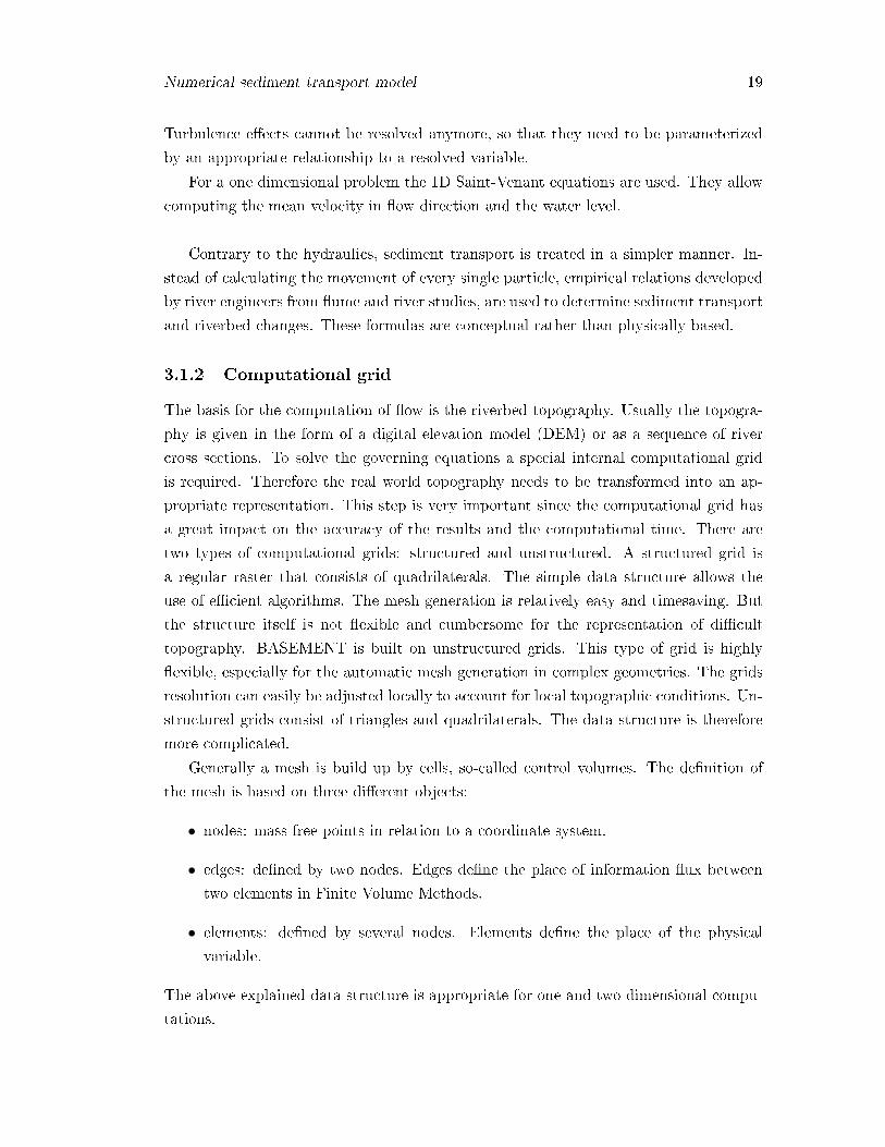
3.1.2 Computational grid
The basis for the computation of �ow is the riverbed topography. Usually the topogra-
phy is given in the form of a digital elevation model (DEM) or as a sequence of river
cross sections. To solve the governing equations a special internal computational grid
is required. Therefore the real world topography needs to be transformed into an ap-
propriate representation. This step is very important since the computational grid has
a great impact on the accuracy of the results and the computational time. There are
two types of computational grids: structured and unstructured. A structured grid is
a regular raster that consists of quadrilaterals. The simple data structure allows the
use of e�cient algorithms. The mesh generation is relatively easy and timesaving. But
the structure itself is not �exible and cumbersome for the representation of di�cult
topography. BASEMENT is built on unstructured grids. This type of grid is highly
�exible, especially for the automatic mesh generation in complex geometries. The grids
resolution can easily be adjusted locally to account for local topographic conditions. Un-
structured grids consist of triangles and quadrilaterals. The data structure is therefore
more complicated.
Generally a mesh is build up by cells, so-called control volumes. The de�nition of
the mesh is based on three di�erent objects:
• nodes: mass free points in relation to a coordinate system.
• edges: de�ned by two nodes. Edges de�ne the place of information �ux between
two elements in Finite Volume Methods.
• elements: de�ned by several nodes. Elements de�ne the place of the physical
variable.
The above explained data structure is appropriate for one and two dimensional compu-
tations.
20
3.1.3 Numerical modules
BASEMENT uses the Finite volume (FV) method to discretize the system of equations.
This method is based on the integration of the equations over a volume that is de�ned by
nodes of grids on the mesh. The equations are therefore discretized in their integral form
and not in the commonly used di�erential form. The FV method is locally and globally
conservative, because of the integration over a volume. To solve the initial value problem
(IVP) three di�erent algorithms are implemented in BASEMENT: exact Riemann solver,
HLL and HLLC approximate Riemann solver. For further details about the numerical
kernel of the model refer to the manual of BASEMENT (Faeh et al., 2006-2008).
3.2 Goals
3.2.1 1d-model BASEchain
The one dimensional tool BASEchain was used to investigate the bed load transport
capacity as well as the evolution of the riverbed in the Pfynwald reach of the Rhone
River. The one dimensional model is not capable of simulating changes of single river
branches or gravel banks, but it is a very useful tool to study changes of the mean
elevation of the riverbed. Additionally a one dimensional numerical sediment transport
model is suitable to investigate the in�uence of variable boundary conditions on the
evolution of the long pro�le and the sediment transport capacity of a river reach.
BASEchain is applied to the whole 8 km long Pfynwald section, starting at the weir
at Susten and ending after the gravel pit at Sierre (�gure 3.2).
3.2.2 2d-model BASEplane
A two dimensional sediment transport model is able to study spatially riverbed changes.
In contrast to a 1d model, a two dimensional model can simulate the behavior of single
river channels and gravel banks. In this study BASEplane is employed to get a more
sophisticated image of river bed changes and sediment transport capacity, in particular
with respect to spatial patterns. Due to the long computational time, BASEplane is
only applied to the uppermost 2 km of the Pfynwald reach (�gure 3.2). Morphologically
this is the most interesting part of the domain, as the con�uence of the Illgraben and the
Rhone is situated in this section. In the present study sediment transport simulations
were limited to the computation of bed load transport. The computation of suspension
load is not addressed in this thesis, because suspension load has limited impact on the
bed forming processes in the Pfynwald reach.
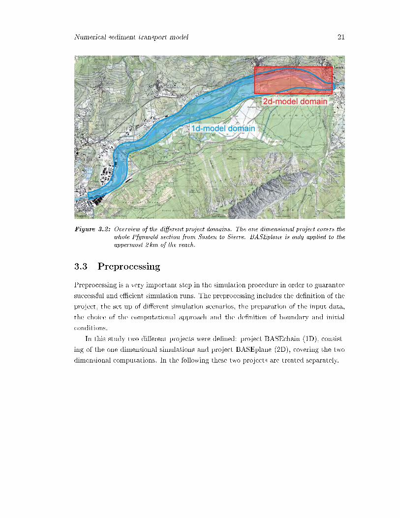
Numerical sediment transport model 21
Figure 3.2: Overview of the di�erent project domains. The one dimensional project covers thewhole Pfynwald section from Susten to Sierre. BASEplane is only applied to theuppermost 2 km of the reach.
3.3 Preprocessing
Preprocessing is a very important step in the simulation procedure in order to guarantee
successful and e�cient simulation runs. The preprocessing includes the de�nition of the
project, the set up of di�erent simulation scenarios, the preparation of the input data,
the choice of the computational approach and the de�nition of boundary and initial
conditions.
In this study two di�erent projects were de�ned: project BASEchain (1D), consist-
ing of the one dimensional simulations and project BASEplane (2D), covering the two
dimensional computations. In the following these two projects are treated separately.
22
3.3.1 Project BASEchain (1D)
Input data
Topography
River cross sections were used as topographic raw data. In the Pfynwald section a
total of 79 cross sections exist, separated in constant gaps of approximately 100m. The
geometry data was provided by the engineering company KBM (KBM SA, 1995-2007).
In order to use the cross sections for a numerical simulation, the geometric data
needs to be transformed into a speci�c topography �le format, saved as a text�le (txt).
This �le contains the topographic description of the cross sections and all the relevant
information for the computations that is related to the riverbed. In this study, the
topographic �le type '�oris' was used. The pure topographic information is given by a
sequence of points, for which the distance from the left border is known. The �le further
speci�es the de�nition of the main channel, the channel bed bottom, the �oodplain, the
bed friction and the soil type. A detailed description of the de�nition of the topography
�le is given in the manual of BASEMENT (Faeh et al., 2006-2008).
Hydrological data
The hydrological data is the most important boundary condition of the model. Hydro-
graphs, steady-state or continuous, or water levels provide the necessary information.
The hydrological data is needed as a sequence of water level [m] or discharge [m3/s] in
times [s]. The �le needs to be saved as a text�le (txt).
Hydrographs can either be implemented in the model as an in�ow boundary condi-
tion or an external source or sink. The in�ow boundary condition is used to simulate
discharge from upstream that enters the study reach. Additional discharge coming from
a tributary is described with a source. Sinks are implemented e.g. in case of water
abstraction by a hydroelectric power plant.
Regarding this study, a continuous hydrograph was used for the in�ow boundary
condition at the weir at Susten. Smaller tributaries (e.g. Illbach, Dala) that drain into
the Rhone in the Pfynwald reach are negligible, so that they are not considered as ad-
ditional sources.
Sediment data
Sedimentological data is needed to characterize the riverbed surface as well as the sub-
surface, which can be eroded by the current. The granulometric size distribution of the
river bed is crucial in terms of sediment transport calculations. Sedimentological proper-
ties of the riverbed are directly written into the command �le of a particular simulation.
The present study uses the sedimentological data that is speci�ed in detail in chapter
Numerical sediment transport model 23
2.2.4. The observed grain size distribution needs to be discretized into classes in order
to use it for the simulation. The resolution of the material composition is determined
by the number of chosen grain classes. Each grain class is de�ned by its mean diameter.
The number of grain classes strongly a�ects the computational e�ort of the simulation;
the more grain classes are taken into account, the more computing power is needed.
Both the number of grain classes and the classi�cation of the grain diameters are very
important with respect to the computation of sediment transport, so that both serve as
a calibration parameter.
In case of a sediment transport computation the boundary condition at the top end
of the model domain has to be known. Additional sediment supply or extraction can
be implemented by means of an external source, respectively sink. In this thesis the
sediment supply, delivered by debris �ows from the Illgraben, is introduced as an exter-
nal source at the corresponding cross section. Gravel extraction at the di�erent gravel
pits is simulated with external sinks. Time, volume and location of the extractions are
known (see chapter 2.2.5), so that sediment extraction hydrographs were de�ned for
every single cross section. The weir at the top end of the Pfynwald section is equipped
with under�ow hydraulic gates, so that the carried sediment from upstream can pass the
weir. As a consequence there is sediment supply to the Pfynwald reach from upstream.
It is implemented by means of a sediment in�ow boundary condition.
Command �le
Before one can execute a simulation with BASEMENT a command �le has to be set
up. This �le contains all the information in order to run the simulation. It is built up
by several blocks. The four main blocks are called 'GEOMETRY', 'HYDRAULICS',
'MORPHOLOGY' and 'OUTPUT'. The 'GEOMETRY' block speci�es the name and
the type of the geometry �le as well as the arrangement of the cross sections, ordered
from upstream to downstream. In the 'HYDRAULICS' block, the boundary and initial
conditions, the friction, possible external sources and some characteristic parameters
of the simulation (e.g. numerical scheme, run time, CFL-number, calibration param-
eters) are de�ned. All the information about the sediment transport computation is
stored in the 'MORPHOLOGY' block. This is namely the grain size distribution of the
bed material, the chosen sediment transport formula and sediment transport calibration
parameters. Finally the 'OUTPUT' block allows you to specify the desired outputs.
24
3.3.2 Project BASEplane (2D)
Input data
Topography
The two dimensional simulation of the hydraulics and the sediment transport of a river
requires a grid that describes the three dimensional topography of the river bed. This
is the most important di�erence to the input data that is needed for a one dimensional
simulation. The mesh �le consists of interconnected node and element data that con-
tain the topographic information. A grid can either be interpolated from river cross
sections, de�ning the channel geometry, or generated with the aid of a digital elevation
model (DEM). The latter is the easier approach and therefore used in this thesis. Still,
there is the need of a so-called preprocessor to generate an appropriate mesh �le. It
is recommended by the developers of BASEMENT to use SMS (Surface Water Mod-
eling System) (Scienti�c Software Group, 2009) as a preprocessor. For this study the
currently available version SMS 10.0 was used.
For the mesh generation a 2m Digital Terrain Model DTM-AV was used as raw
data. This data is produced by Swisstopo (Bundesamt für Landestopographie Swisstopo,
2005b). It represents the topography of the Earth's surface without vegetation and
buildings. The model is based on high precision laser scanning (LIDAR) from airplanes,
and the accuracy is +/- 0.5m. To reduce the amount of data, the spatial resolution of
the DEM was decreased to 4m. The accuracy is still good enough for the purpose of
simulations of sediment transport.
The use of an orthophoto or a detailed map is very helpful in the process of mesh
generation. The geometrically corrected picture or the map can be imported into SMS
and then used as a background image. This study used an orthophoto taken from
Swisstopo in summer 2005 (Bundesamt für Landestopographie Swisstopo, 2005a).
An automatic triangulation of the data points would be the easiest way to generate
a mesh, but this will end up with some unfavorable element shapes and con�gurations
(e.g. unnatural �attening of the terrain). Therefore the mesh is rather generated using
a conceptual model as a basis for the triangulation. This conceptual model is built up
with the aid of the aerial photo. The boundaries of the model domain are de�ned as
signi�cant terrain features, and consequently the structure of the model domain terrain
is prede�ned. Besides, the spatial resolution can be modulated locally, by assigning the
number of nodes along a signi�cant terrain feature or boundary. The use of a conceptual
model to triangulate the data points results in a mesh that allows for variability in the
spatial resolution and that contains edges that follow along the centerlines, shoulders,
and bathymetry intersections. The generated mesh still needs to be checked and locally
adjusted. Moreover one has to de�ne the material type of the elements to account for
Numerical sediment transport model 25
spatial di�erences in the composition of the riverbed and the channel bed roughness (e.g.
channel bed, �oodplain, embankments). Not to forget is the conversion of quadratic
elements (six node triangles and eight node quadrilaterals) to linear elements (three
node triangles and four node quadrilaterals) in order to use the grid for a simulation
with BASEMENT. Finally the mesh has to be saved as a 2dm �le.
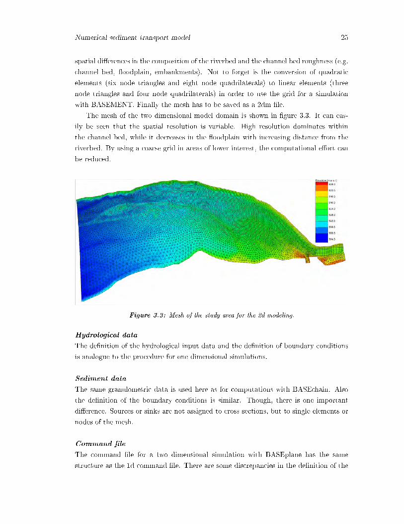
The mesh of the two dimensional model domain is shown in �gure 3.3. It can eas-
ily be seen that the spatial resolution is variable. High resolution dominates within
the channel bed, while it decreases in the �oodplain with increasing distance from the
riverbed. By using a coarse grid in areas of lower interest, the computational e�ort can
be reduced.
Figure 3.3: Mesh of the study area for the 2d modeling.
Hydrological data
The de�nition of the hydrological input data and the de�nition of boundary conditions
is analogue to the procedure for one dimensional simulations.
Sediment data
The same granulometric data is used here as for computations with BASEchain. Also
the de�nition of the boundary conditions is similar. Though, there is one important
di�erence. Sources or sinks are not assigned to cross sections, but to single elements or
nodes of the mesh.
Command �le
The command �le for a two dimensional simulation with BASEplane has the same
structure as the 1d command �le. There are some discrepancies in the de�nition of the

26
geometry, the boundary conditions and the channel bed for sediment transport compu-
tations.
Chapter 4
Model calibration
4.1 Project BASEchain (1D)
Generally the model needs to be calibrated in a two step procedure. First, one has to
calibrate the hydraulic part of the model, meaning that only the water �ow through
the study reach is simulated. Observed �ood marks are usually taken as a reference
value. The simulated water levels need then to be �tted to the observed �ood marks,
by changing the roughness coe�cient of the channel bed. Due to the use of quite
sophisticated physical models for the hydraulic computations, on the one hand the need
for a hydraulic calibration is limited and on the other hand the number of calibration
parameters is inherently small. Since it is very complicated to measure the roughness of
a riverbed, it is obvious that the roughness coe�cient is the most sensitive and important
calibration parameter in hydraulic simulations.
Unfortunately there is no �ood mark observation data available for the Pfynwald river
reach. For that reason the hydraulic part of BASEchain was not calibrated. That is
of no consequence, concerning the sediment transport simulation, since the calibration
potential of the sediment transport computation is much larger than the hydraulics.
The formulas for sediment transport are primarily based on empirics, so that a model
calibration is essential.
There is very good data available for the calibration of BASEchain concerning sed-
iment transport in the Pfynwald reach. The model was calibrated on the basis of to-
pographic data for the period of 12 years from October 1995 to October 2007 that was
surveyed annually by the engineering company KBM (see chapter 2.2.5). The goal was
to �t the simulated riverbed changes to the observed changes. In addition, the simu-
lated bed load transport is compared to the one that was reconstructed on the basis of
observations in the Pfynwald reach and sediment transport simulations in the adjacent
river sections.
27
28
4.1.1 Input data
The topographic data from October 1995 was used as the starting position for the
calibration of the model. The channel bed geometry observed in 2007 was then applied
as a reference to evaluate to models performance.
The granulometric composition of the riverbed was described by means of particle
size distributions that were measured by Hunziker, Zarn & Partner AG (2001) and Jäggi
(1988). To characterize the grain size distribution of the debris �ow material, the data
that was surveyed in the scope of this study was used.
The in�ow-hydrograph used for the calibration was computed according to the
method described in chapter 2.2.1. During low �ows generally no sediment is trans-
ported in the Rhone, so that low discharges were omitted in the hydrograph. Normally
the initiation of sediment transport coincidences with the breakup of the armored layer.
The corresponding stress to the riverbed, expressed as a discharge, is called QD. Ac-
cording to Hunziker, Zarn & Partner AG (2001) and Jäggi (1988) sediment transport is
initiated at a discharge that exceeds 150 to 200m3/s. To remain considerably below this
critical stream�ow a discharge of 100m3/s was chosen as a threshold for the hydrograph.
Due to the shortening of the e�ective duration of the hydrograph, computational time
can be saved.
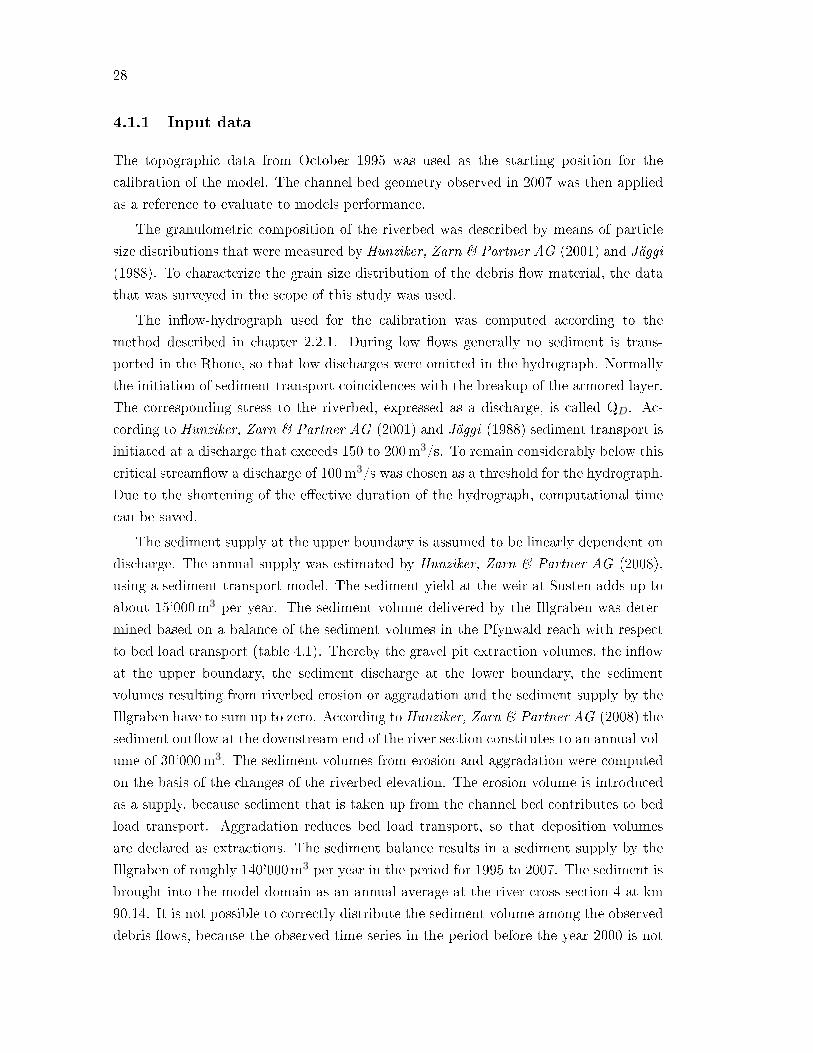
The sediment supply at the upper boundary is assumed to be linearly dependent on
discharge. The annual supply was estimated by Hunziker, Zarn & Partner AG (2008),
using a sediment transport model. The sediment yield at the weir at Susten adds up to
about 15'000m3 per year. The sediment volume delivered by the Illgraben was deter-
mined based on a balance of the sediment volumes in the Pfynwald reach with respect
to bed load transport (table 4.1). Thereby the gravel pit extraction volumes, the in�ow
at the upper boundary, the sediment discharge at the lower boundary, the sediment
volumes resulting from riverbed erosion or aggradation and the sediment supply by the
Illgraben have to sum up to zero. According to Hunziker, Zarn & Partner AG (2008) the
sediment out�ow at the downstream end of the river section constitutes to an annual vol-
ume of 30'000m3. The sediment volumes from erosion and aggradation were computed
on the basis of the changes of the riverbed elevation. The erosion volume is introduced
as a supply, because sediment that is taken up from the channel bed contributes to bed
load transport. Aggradation reduces bed load transport, so that deposition volumes
are declared as extractions. The sediment balance results in a sediment supply by the
Illgraben of roughly 140'000m3 per year in the period for 1995 to 2007. The sediment is
brought into the model domain as an annual average at the river cross section 4 at km
90.14. It is not possible to correctly distribute the sediment volume among the observed
debris �ows, because the observed time series in the period before the year 2000 is not
Model calibration 29
complete (see table A.2).
Table 4.1: Sediment balance in the Pfynwald reach for the period of 1996 to 2007 regarding bedload transport. Volumes are given in m3/a including porosity.
supply extraction/discharge
total 1995-2007 annual total 1995-2007 annual
upper boundary 180'000 15'000
lower boundary -360'000 -30'000
gravel extraction -1'651'336 -137'611
bed erosion 309'842 25'820
aggradation -178'345 -14'862
subtotal 361'649 30'137 -2'325'308 -193'776
Illgraben 1'699'839 141'653
The gravel pits were implemented to the model as external sinks, distributed along
the reach according to table 2.2. The extraction volumes were simulated as constant
annual extraction rates. Because all of the above mentioned sediment volumes include
porosity, they need to be transformed into pure sediment volumes in order to satisfy the
requirements of BASEMENT. A constant porosity of 0.37 was applied to convert the
volumes.
The initial condition was de�ned using an initial state stored in a separate �le. This
�le describes the exact initial situation of the hydraulic conditions in the channel. It was
obtained by means of a hydraulic simulation with a steady-state hydrograph of 100m3/s.
The hydraulic simulation was started with the initial condition 'dry' and it was run as
long as a steady state was reached.
4.1.2 Calibration parameters
The models performance was improved by calibrating three di�erent parameters:
• Upwind
• Active layer height
• Sediment composition
Upwind
The parameter 'upwind' determines how the bed load �ux at the cell interface between
two cross sections is calculated. The calculation of bed load transport takes place in
30
the cross sections, since all the data, which is needed to compute the �ux is available
there. The parameter 'upwind' de�nes which data is used to interpolate the bed load
�ux in the cell interface. A value between 0 and 1 can be assigned to the parameter.
If upwind is set to 1, only the upstream cross section is considered, in case of a 0 the
value of the downstream section is assigned to the �ux. 'upwind' is a very important
calibration parameter with respect to the stability of the simulation.
Active layer height
The active layer height de�nes the uppermost layer of the riverbed in which the im-
portant processes of sediment transport take place. By enlarging this height, sediment
transport rates generally increase, because more bed material is exposed to the �ow and
the applied shear stress. The active layer height is constant in the whole model domain;
it cannot be adjusted for speci�c cross sections.
Sediment composition
The grain size distribution of the riverbed material was measured by means of line sur-
veys or sieving analysis. To use this data for the numerical simulation it needs to be
discretized as mentioned earlier (chapter 3.3.1). Based on the observed particle size
distribution, one has to de�ne the desired grain classes with their corresponding mean
diameters. The easiest approach to characterize the channel bed material is to use
one single mean diameter. However, a great disadvantage of single grain simulations
is that bed material sorting e�ects cannot be captured, so that the model is not able
to simulate bed armoring. In case of the Pfynwald reach it is very important to ac-
count for the forming and destroying of the armored layer. For a single grain simulation
BASEMENT provides two methods to arti�cially introduce a protection layer. Either
a critical shear stress (τcr) of the protection layer or the d90 grain diameter of the bed
armoring layer can be de�ned. In case of the critical shear stress, erosion of the river
bed starts if the stress is exceeded. Using the d90 grain diameter to characterize the
armored layer, �rst the model needs to compute the dimensionless critical shear stress
of the bed (θcr). If the stress induced by the �ow exceeds the dimensionless critical shear
stress of the riverbed, erosion of the channel bed begins. If the armored layer is eroded
once, it cannot be built up again. In this study the �rst approach using a critical shear
stress was applied to account for a protection layer. The employed critical shear stress
was computed on the basis of the d90 according to �gure 4.1 using the following formula:
τcr = θcr,armor · (s− 1) dm = θcr
(d90
dm
)2/3
· (s− 1) dm
Model calibration 31
with d90 as the speci�ed d90 grain diameter of the substrate, dm is the mean diameter of
the riverbed material, θcr corresponds to the critical shear stress of the substrate (here
θcr = 0.05) and s denotes the relative density of the gravel (ρs/ρw = 1.65).
To consider bed material sorting e�ects it is advisable to perform multiple grain size
simulations. In this thesis the e�ect of the use of multiple grain sizes was studied in
the course of the model calibration. Additionally to the single grain size runs, simula-
tions with two di�erent numbers of grain classes were performed, using either 5 or 10
grain classes to specify the substrate. Depending on the number of used grain classes,
di�erent approaches for the computation of sediment transport were used. In case of a
single grain simulation the sediment transport formula of Meyer-Peter Müller (MPM)
was applied. For multiple grain class simulations the revised form of the MPM formula
after Hunziker (MPMH) was applied.
Single grain simulation
In case of a single grain simulation one mean particle diameter was used to characterize
the riverbed as well as all the material that is supplied to or extracted from the Pfynwald
river reach. The mean grain size is the parameter that needs to be adjusted in order to
improve the models performance. According to the observations of the granulometric
composition of Hunziker, Zarn & Partner AG (2001) and Jäggi (1988) the mean particle
diameter of the riverbed in the Pfynwald reach adds up to about 100mm. Hence a �rst
simulation was run using this value. Subsequently the mean grain size was adjusted to
achieve a better �t of the model results.
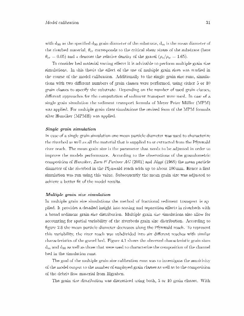
Multiple grain size simulation
In multiple grain size simulations the method of fractional sediment transport is ap-
plied. It provides a detailed insight into sorting and separation e�ects in riverbeds with
a broad sediment grain size distribution. Multiple grain size simulations also allow for
accounting for spatial variability of the riverbeds grain size distribution. According to
�gure 2.6 the mean particle diameter decreases along the Pfynwald reach. To represent
this variability, the river reach was subdivided into six di�erent reaches with similar
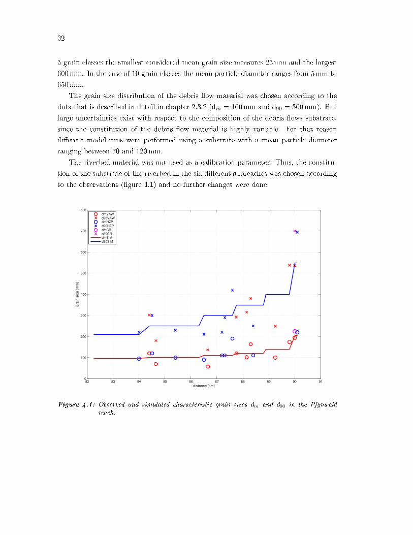
characteristics of the gravel bed. Figure 4.1 shows the observed characteristic grain sizes
dm and d90 as well as those that were used to characterize the composition of the channel
bed in the simulation runs.
The goal of the multiple grain size calibration runs was to investigate the sensitivity
of the model output to the number of employed grain classes as well as to the composition
of the debris �ow material from Illgraben.
The grain size distribution was discretized using both, 5 or 10 grain classes. With
32
5 grain classes the smallest considered mean grain size measures 25mm and the largest
600mm. In the case of 10 grain classes the mean particle diameter ranges from 5mm to
650mm.
The grain size distribution of the debris �ow material was chosen according to the
data that is described in detail in chapter 2.3.2 (dm = 100mm and d90 = 300mm). But
large uncertainties exist with respect to the composition of the debris �ows substrate,
since the constitution of the debris �ow material is highly variable. For that reason
di�erent model runs were performed using a substrate with a mean particle diameter
ranging between 70 and 120mm.
The riverbed material was not used as a calibration parameter. Thus, the constitu-
tion of the substrate of the riverbed in the six di�erent subreaches was chosen according
to the observations (�gure 4.1) and no further changes were done.
82 83 84 85 86 87 88 89 90 910
100
200
300
400
500
600
700
800
distance [km]
gra
in s
ize
[m
m]
dmVAWd90VAWdmHZPd90HZPdmCRd90CRdmSIMd90SIM
Figure 4.1: Observed and simulated characteristic grain sizes dm and d90 in the Pfynwaldreach.
Model calibration 33
4.1.3 Calibration results
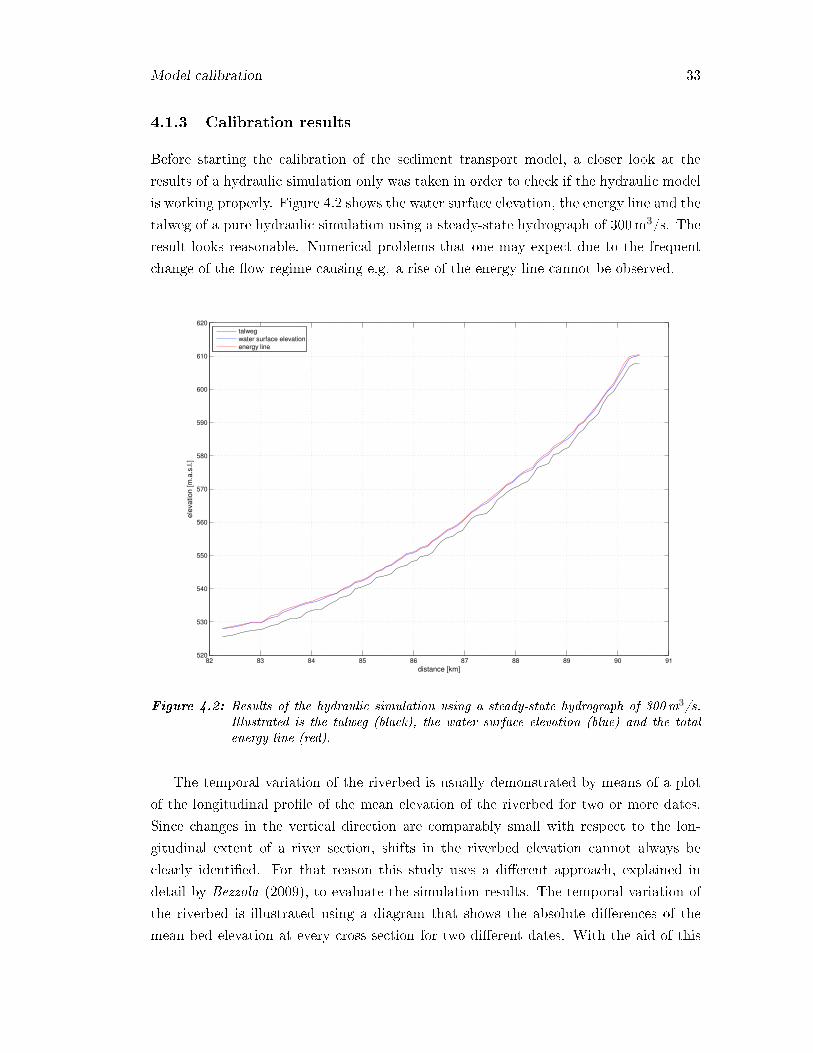
Before starting the calibration of the sediment transport model, a closer look at the
results of a hydraulic simulation only was taken in order to check if the hydraulic model
is working properly. Figure 4.2 shows the water surface elevation, the energy line and the
talweg of a pure hydraulic simulation using a steady-state hydrograph of 300m3/s. The
result looks reasonable. Numerical problems that one may expect due to the frequent
change of the �ow regime causing e.g. a rise of the energy line cannot be observed.
82 83 84 85 86 87 88 89 90 91520
530
540
550
560
570
580
590
600
610
620
distance [km]
ele
va
tio
n [m
.a.s
.l.]
talweg
water surface elevation
energy line
Figure 4.2: Results of the hydraulic simulation using a steady-state hydrograph of 300m3/s.Illustrated is the talweg (black), the water surface elevation (blue) and the totalenergy line (red).
The temporal variation of the riverbed is usually demonstrated by means of a plot
of the longitudinal pro�le of the mean elevation of the riverbed for two or more dates.
Since changes in the vertical direction are comparably small with respect to the lon-
gitudinal extent of a river section, shifts in the riverbed elevation cannot always be
clearly identi�ed. For that reason this study uses a di�erent approach, explained in
detail by Bezzola (2009), to evaluate the simulation results. The temporal variation of
the riverbed is illustrated using a diagram that shows the absolute di�erences of the
mean bed elevation at every cross section for two di�erent dates. With the aid of this
34
plot a so-called transport diagram is computed. On the basis of the mean bed elevation
for two di�erent times, the volumes of erosion and deposition at every cross section are
calculated. Adding the computed volumes along the considered river section yields the
bed load transport in the form of a transport diagram. Sediment that enters the river
e.g. through tributaries or gravel that is extracted at gravel pits needs to be added to
the transport diagram additionally. For that purpose the extraction volumes as well
as the sediment supply have to be known. It is very important that all the sediment
volumes are declared consistently with respect to porosity. Particularly in the case of
sediment volumes originating from numerical sediment transport computations one has
to make sure how porosity is considered. While the volumes of erosion or deposition,
gravel extraction and sediment supply already account for porosity, sediment volumes
stemming from sediment transport simulations generally estimate pure sediment mass.
In this thesis the sediment quantity is always given as a volume including porosity.
The transport diagram is an excellent tool to get an idea of the sediment budget and
the general transport behavior of a river. In case the sediment in�ow or out�ow of the
considered river section is known accurately enough, the transport diagram even allows
determining sediment transport quantitatively.
A decreasing curve in the transport diagram corresponds to aggradation or sediment
extractions in the riverbed. Conversely erosion provokes a rising curve. Locally restricted
sediment supply (e.g. tributary) or extraction (e.g. gravel pit) causes an abrupt increase,
respectively a sudden decrease of bed load transport.
Upwind
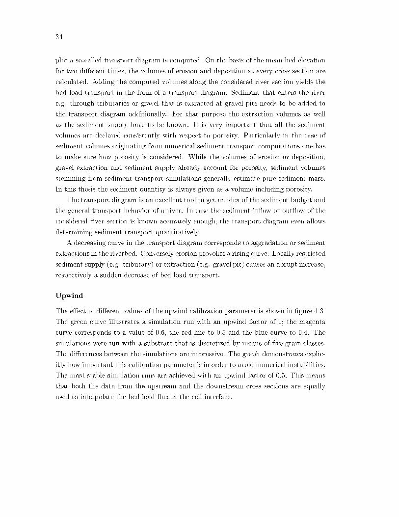
The e�ect of di�erent values of the upwind calibration parameter is shown in �gure 4.3.
The green curve illustrates a simulation run with an upwind factor of 1; the magenta
curve corresponds to a value of 0.6, the red line to 0.5 and the blue curve to 0.4. The
simulations were run with a substrate that is discretized by means of �ve grain classes.
The di�erences between the simulations are impressive. The graph demonstrates explic-
itly how important this calibration parameter is in order to avoid numerical instabilities.
The most stable simulation runs are achieved with an upwind factor of 0.5. This means
that both the data from the upstream and the downstream cross sections are equally
used to interpolate the bed load �ux in the cell interface.
Model calibration 35
82 83 84 85 86 87 88 89 90 91-4
-3
-2
-1
0
1
2
3
4
5
6Changes in riverbed elevation
distance [km]
be
d c
ha
ng
e [m
]
DZobs
DZsim
upw 0.4
DZsim
upw 0.5
DZsim
upw 0.6
DZsim
upw 1.0
82 83 84 85 86 87 88 89 90 91-100,000
-50,000
0
50,000
100,000
150,000
200,000Transport diagram
distance [km]
be
d lo
ad
tra
nsp
ort
[m
3/a
]
Qbobs
Qbsim
upw 0.4
Qbsim
upw 0.5
Qbsim
upw 0.6
Qbsim
upw 1.0
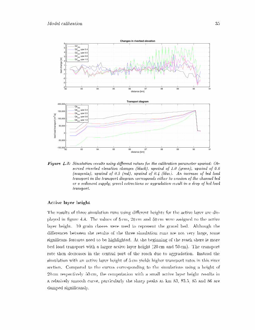
Figure 4.3: Simulation results using di�erent values for the calibration parameter upwind: Ob-served riverbed elevation changes (black), upwind of 1.0 (green), upwind of 0.6(magenta), upwind of 0.5 (red), upwind of 0.4 (blue). An increase of bed loadtransport in the transport diagram corresponds either to erosion of the channel bedor a sediment supply; gravel extractions or aggradation result in a drop of bed loadtransport.
Active layer height
The results of three simulation runs using di�erent heights for the active layer are dis-
played in �gure 4.4. The values of 5 cm, 20 cm and 50 cm were assigned to the active
layer height. 10 grain classes were used to represent the gravel bed. Although the
di�erences between the results of the three simulation runs are not very large, some
signi�cant features need to be highlighted. At the beginning of the reach there is more
bed load transport with a larger active layer height (20 cm and 50 cm). The transport
rate then decreases in the central part of the reach due to aggradation. Instead the
simulation with an active layer height of 5 cm yields higher transport rates in this river
section. Compared to the curves corresponding to the simulations using a height of
20 cm respectively 50 cm, the computation with a small active layer height results in
a relatively smooth curve, particularly the sharp peaks at km 83, 83.5, 85 and 86 are
damped signi�cantly.
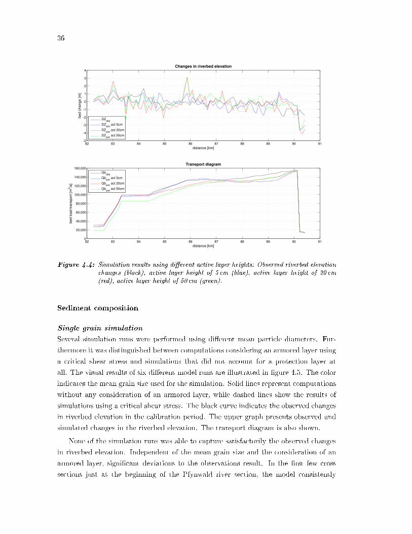
36
82 83 84 85 86 87 88 89 90 91-5
-4
-3
-2
-1
0
1
2
3
4Changes in riverbed elevation
distance [km]
be
d c
ha
ng
e [m
]
DZobs
DZsim
act 5cm
DZsim
act 20cm
DZsim
sct 50cm
82 83 84 85 86 87 88 89 90 910
20,000
40,000
60,000
80,000
100,000
120,000
140,000
160,000Transport diagram
distance [km]
be
d lo
ad
tra
nsp
ort
[m
3/a
]
Qbobs
Qbsim
act 5cm
Qbsim
act 20cm
Qbsim
act 50cm
Figure 4.4: Simulation results using di�erent active layer heights: Observed riverbed elevationchanges (black), active layer height of 5 cm (blue), active layer height of 20 cm(red), active layer height of 50 cm (green).
Sediment composition
Single grain simulation
Several simulation runs were performed using di�erent mean particle diameters. Fur-
thermore it was distinguished between computations considering an armored layer using
a critical shear stress and simulations that did not account for a protection layer at
all. The visual results of six di�erent model runs are illustrated in �gure 4.5. The color
indicates the mean grain size used for the simulation. Solid lines represent computations
without any consideration of an armored layer, while dashed lines show the results of
simulations using a critical shear stress. The black curve indicates the observed changes
in riverbed elevation in the calibration period. The upper graph presents observed and
simulated changes in the riverbed elevation. The transport diagram is also shown.
None of the simulation runs was able to capture satisfactorily the observed changes
in riverbed elevation. Independent of the mean grain size and the consideration of an
armored layer, signi�cant deviations to the observations result. In the �rst few cross
sections just at the beginning of the Pfynwald river section, the model consistently
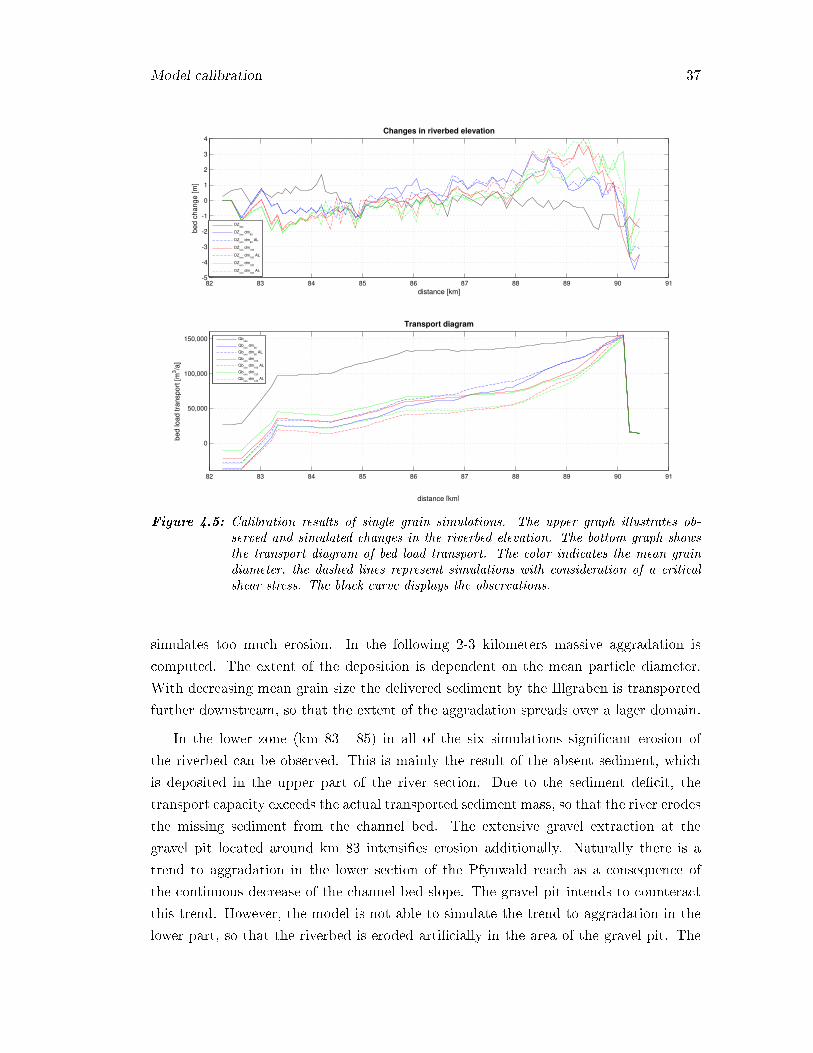
Model calibration 37
82 83 84 85 86 87 88 89 90 91-5
-4
-3
-2
-1
0
1
2
3
4Changes in riverbed elevation
distance [km]
be
d c
ha
ng
e [m
]
DZobs
DZsim
dm80
DZsim
dm80
AL
DZsim
dm100
DZsim
dm100
AL
DZsim
dm120
DZsim
dm120
AL
82 83 84 85 86 87 88 89 90 91
0
50,000
100,000
150,000
Transport diagram
distance [km]
be
d lo
ad
tra
nsp
ort
[m
3/a
]
Qb
obs
Qbsim
dm80
Qbsim
dm80
AL
Qbsim
dm100
Qbsim
dm100
AL
Qbsim
dm120
Qbsim
dm120
AL
Figure 4.5: Calibration results of single grain simulations. The upper graph illustrates ob-served and simulated changes in the riverbed elevation. The bottom graph showsthe transport diagram of bed load transport. The color indicates the mean graindiameter, the dashed lines represent simulations with consideration of a criticalshear stress. The black curve displays the observations.
simulates too much erosion. In the following 2-3 kilometers massive aggradation is
computed. The extent of the deposition is dependent on the mean particle diameter.
With decreasing mean grain size the delivered sediment by the Illgraben is transported
further downstream, so that the extent of the aggradation spreads over a lager domain.
In the lower zone (km 83 - 85) in all of the six simulations signi�cant erosion of
the riverbed can be observed. This is mainly the result of the absent sediment, which
is deposited in the upper part of the river section. Due to the sediment de�cit, the
transport capacity exceeds the actual transported sediment mass, so that the river erodes
the missing sediment from the channel bed. The extensive gravel extraction at the
gravel pit located around km 83 intensi�es erosion additionally. Naturally there is a
trend to aggradation in the lower section of the Pfynwald reach as a consequence of
the continuous decrease of the channel bed slope. The gravel pit intends to counteract
this trend. However, the model is not able to simulate the trend to aggradation in the
lower part, so that the riverbed is eroded arti�cially in the area of the gravel pit. The

38
magnitude of the channel bed erosion decreases with smaller mean particle diameter,
because more sediment is transported to the lower areas of the Pfynwald reach.
The transport diagram re�ects the riverbed changes quite well. The massive aggra-
dation at the beginning of the reach causes a dramatic drop of bed load transport.
Roughly two-thirds of the supplied sediment by the Illgraben is deposited within the
�rst two kilometers after the con�uence with the Illgraben. In reality bed load trans-
port remains at a very high rate, so that most of the debris �ow material is transported
further downstream. On average, the computations of bed load transport result in a
de�cit of about 60'000 to 70'000m3/a in the Pfynwald reach. In the lowest section of
the reach the model computes even a negative bed load transport rate, which seems to
be quite strange, just as the fact that the simulation with a mean grain diameter of
80mm (blue curve) yields the largest sediment transport de�cit. One actually would
expect the opposite, meaning that coarser gravel would result in a decrease of transport
capacity. These e�ects remain unexplained.
The use of a critical shear stress a�ects the simulation results only marginally. In
general, the use of a critical shear stress ampli�es the magnitude of the aggradation.
The e�ect is more pronounced, the larger the considered mean particle diameter is.
Multiple grain size simulation
In the following the results of a couple of simulations using either di�erent numbers of
grain classes or variable compositions of the debris �ow material are presented.
Figure 4.6 shows the e�ect of using di�erentmultiple grain classes. The results of
a single grain simulation (blue) and two multigrain simulations (5 grain classes: red, 10
grain classes: green) are illustrated. Again all of the simulations show massive erosion
at the beginning of the reach. Most probably this is caused by e�ects triggered by the
de�nition of the upper boundary condition. The main di�erences occur in the river
section that follows after the con�uence of the Illgraben. In principle, the magnitude of
the aggradation increases with decreasing number of grain classes. While in case of the
10 grain class simulation the riverbed elevation does not show a signi�cant change in
this area, the single grain simulation results in very large deposition of up to 3 meters.
If one also considers the huge channel width in this area (100 to 250m) the deposited
sediment volume is substantial. Nearly all of the supplied sediment by the Illgraben is
deposited in this river section. Beside the vertical shift, all of the three curves show
a similar progression in the �rst two kilometers. This indicates a consistent model
behavior, meaning that simulated channel change is caused by the di�erent model set
ups and not by randomness or numerical instabilities.
The simulation using 10 grain class generally �ts the observations best. No aggrada-
tion at all is computed in the con�uence area. This means that the computed transport
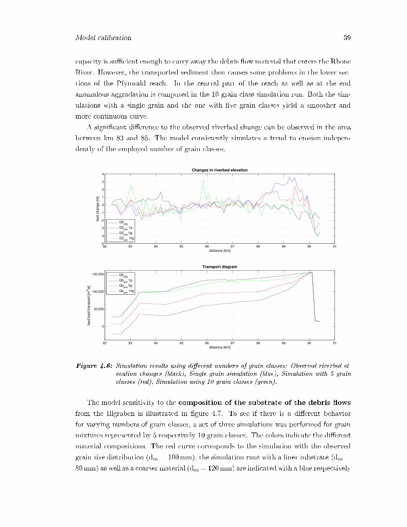
Model calibration 39
capacity is su�cient enough to carry away the debris �ow material that enters the Rhone
River. However, the transported sediment then causes some problems in the lower sec-
tions of the Pfynwald reach. In the central part of the reach as well as at the end
anomalous aggradation is computed in the 10 grain class simulation run. Both the sim-
ulations with a single grain and the one with �ve grain classes yield a smoother and
more continuous curve.
A signi�cant di�erence to the observed riverbed change can be observed in the area
between km 83 and 85. The model consistently simulates a trend to erosion indepen-
dently of the employed number of grain classes.
82 83 84 85 86 87 88 89 90 91-5
-4
-3
-2
-1
0
1
2
3
4Changes in riverbed elevation
distance [km]
be
d c
ha
ng
e [m
]
DZobs
DZsim
1g
DZsim
5g
DZsim
10g
82 83 84 85 86 87 88 89 90 91
0
50,000
100,000
150,000
Transport diagram
distance [km]
be
d lo
ad
tra
nsp
ort
[m
3/a
]
Qbobs
Qbsim
1g
Qbsim
5g
Qbsim
10g
Figure 4.6: Simulation results using di�erent numbers of grain classes: Observed riverbed el-evation changes (black), Single grain simulation (blue), Simulation with 5 grainclasses (red), Simulation using 10 grain classes (green).
The model sensitivity to the composition of the substrate of the debris �ows
from the Illgraben is illustrated in �gure 4.7. To see if there is a di�erent behavior
for varying numbers of grain classes, a set of three simulations was performed for grain
mixtures represented by 5 respectively 10 grain classes. The colors indicate the di�erent
material compositions. The red curve corresponds to the simulation with the observed
grain size distribution (dm = 100mm), the simulation runs with a �ner substrate (dm =
80mm) as well as a coarser material (dm = 120mm) are indicated with a blue respectively
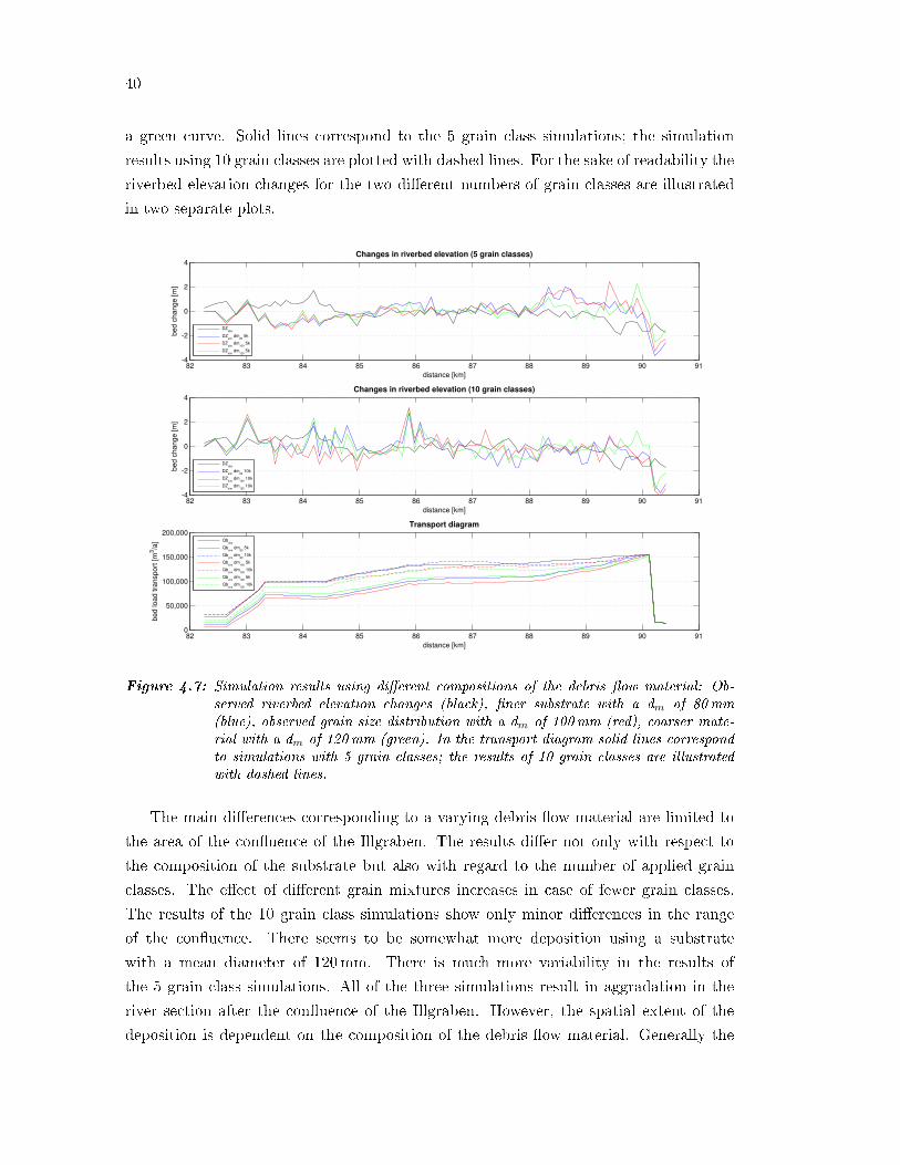
40
a green curve. Solid lines correspond to the 5 grain class simulations; the simulation
results using 10 grain classes are plotted with dashed lines. For the sake of readability the
riverbed elevation changes for the two di�erent numbers of grain classes are illustrated
in two separate plots.
82 83 84 85 86 87 88 89 90 91-4
-2
0
2
4Changes in riverbed elevation (5 grain classes)
distance [km]
bed c
hange [m
]
DZobs
DZsim
dm80
5k
DZsim
dm100
5k
DZsim
dm120
5k
82 83 84 85 86 87 88 89 90 91-4
-2
0
2
4Changes in riverbed elevation (10 grain classes)
distance [km]
bed c
hange [m
]
DZobs
DZsim
dm80
10k
DZsim
dm100
10k
DZsim
dm120
10k
82 83 84 85 86 87 88 89 90 910
50,000
100,000
150,000
200,000Transport diagram
distance [km]
bed load tra
nsport
[m
3/a
]
Qb
obs
Qbsim
dm80
5k
Qbsim
dm80
10k
Qbsim
dm100
5k
Qbsim
dm100
10k
Qbsim
dm120
5k
Qbsim
dm120
10k
Figure 4.7: Simulation results using di�erent compositions of the debris �ow material: Ob-served riverbed elevation changes (black), �ner substrate with a dm of 80mm(blue), observed grain size distribution with a dm of 100mm (red), coarser mate-rial with a dm of 120mm (green). In the transport diagram solid lines correspondto simulations with 5 grain classes; the results of 10 grain classes are illustratedwith dashed lines.
The main di�erences corresponding to a varying debris �ow material are limited to
the area of the con�uence of the Illgraben. The results di�er not only with respect to
the composition of the substrate but also with regard to the number of applied grain
classes. The e�ect of di�erent grain mixtures increases in case of fewer grain classes.
The results of the 10 grain class simulations show only minor di�erences in the range
of the con�uence. There seems to be somewhat more deposition using a substrate
with a mean diameter of 120mm. There is much more variability in the results of
the 5 grain class simulations. All of the three simulations result in aggradation in the
river section after the con�uence of the Illgraben. However, the spatial extent of the
deposition is dependent on the composition of the debris �ow material. Generally the
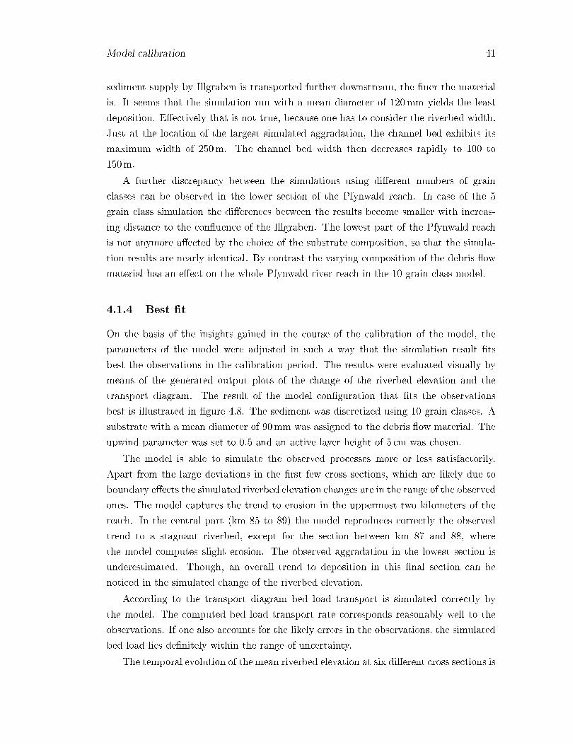
Model calibration 41
sediment supply by Illgraben is transported further downstream, the �ner the material
is. It seems that the simulation run with a mean diameter of 120mm yields the least
deposition. E�ectively that is not true, because one has to consider the riverbed width.
Just at the location of the largest simulated aggradation, the channel bed exhibits its
maximum width of 250m. The channel bed width then decreases rapidly to 100 to
150m.
A further discrepancy between the simulations using di�erent numbers of grain
classes can be observed in the lower section of the Pfynwald reach. In case of the 5
grain class simulation the di�erences between the results become smaller with increas-
ing distance to the con�uence of the Illgraben. The lowest part of the Pfynwald reach
is not anymore a�ected by the choice of the substrate composition, so that the simula-
tion results are nearly identical. By contrast the varying composition of the debris �ow
material has an e�ect on the whole Pfynwald river reach in the 10 grain class model.
4.1.4 Best �t
On the basis of the insights gained in the course of the calibration of the model, the
parameters of the model were adjusted in such a way that the simulation result �ts
best the observations in the calibration period. The results were evaluated visually by
means of the generated output plots of the change of the riverbed elevation and the
transport diagram. The result of the model con�guration that �ts the observations
best is illustrated in �gure 4.8. The sediment was discretized using 10 grain classes. A
substrate with a mean diameter of 90mm was assigned to the debris �ow material. The
upwind parameter was set to 0.5 and an active layer height of 5 cm was chosen.
The model is able to simulate the observed processes more or less satisfactorily.
Apart from the large deviations in the �rst few cross sections, which are likely due to
boundary e�ects the simulated riverbed elevation changes are in the range of the observed
ones. The model captures the trend to erosion in the uppermost two kilometers of the
reach. In the central part (km 85 to 89) the model reproduces correctly the observed
trend to a stagnant riverbed, except for the section between km 87 and 88, where
the model computes slight erosion. The observed aggradation in the lowest section is
underestimated. Though, an overall trend to deposition in this �nal section can be
noticed in the simulated change of the riverbed elevation.
According to the transport diagram bed load transport is simulated correctly by
the model. The computed bed load transport rate corresponds reasonably well to the
observations. If one also accounts for the likely errors in the observations, the simulated
bed load lies de�nitely within the range of uncertainty.
The temporal evolution of the mean riverbed elevation at six di�erent cross sections is

42
82 83 84 85 86 87 88 89 90 91-5
-4
-3
-2
-1
0
1
2Changes in riverbed elevation
distance [km]
be
d c
ha
ng
e [m
]
DZobs
DZbestfit
82 83 84 85 86 87 88 89 90 910
20,000
40,000
60,000
80,000
100,000
120,000
140,000
160,000
180,000Transport diagram
distance [km]
be
d lo
ad
tra
nsp
ort
[m
3/a
]
Qbobs
Qbbestfit
Figure 4.8: Simulation results of the model con�guration that �ts the observations best. Multi-grain simulation with 10 grain classes; debris �ow material with a mean particlediameter of 90mm; upwind parameter = 0.5; active layer height = 5 cm.
shown in �gure 4.9. The observations are presented in black, while the simulated riverbed
elevation is illustrated with a red color. With the aid of these plots, one can evaluate
the performance of the model in capturing the observed progression of the riverbed.
Generally there is quite a large discrepancy between the two curves, independently of
the considered cross section. The best match results at cross section 4F, which is located
just at the end of the Pfynwald reach. In cross sections 30, 46 and 63 the model even
computes the evolution of the channel bed elevation in a converse manner. Concerning
the cross section at the con�uence of the Illgraben (CS 4), the model is able to capture
the long-term trend to a subsidence of the riverbed, but it does not reproduce the massive
aggradation in the years 1998 and 1999.
Looking just at the observed progression of the riverbed, a pulsation of the channel
bed elevation can be identi�ed. The large aggradation at cross section 4 in the year
1998 propagates downstream and shows up in the graph corresponding to cross section
16 in the year 2001. The magnitude of the absolute riverbed change has decreased from
2.5m at cross section 4 to 1.5m at cross section 16. With increasing distance to the
con�uence of the Illgraben it becomes more di�cult to allocate a particular detail to its

Model calibration 43
initial feature at cross section 4, because the di�erent pulses are damped and they may
also interfere with each other. However, a pulsation of the riverbed can also be observed
further downstream as the plots of the cross sections 46 and 63 illustrate very well.
1994 1996 1998 2000 2002 2004 2006 2008603
604
605
606
607
608CS 4 (km 90.120)
time [years]
mean r
iverb
ed e
levation [m
.a.s
.l.]
RBobs
RBbestfit
1994 1996 1998 2000 2002 2004 2006 2008582
582.5
583
583.5
584CS 16 (km 88.937)
time [years]
mean r
iverb
ed e
levation [m
.a.s
.l.]
RBobs
RBbestfit
1994 1996 1998 2000 2002 2004 2006 2008565.5
566
566.5
567CS 30 (km 87.539)
time [years]
mean r
iverb
ed e
levation [m
.a.s
.l.]
RBobs
RBbestfit
1994 1996 1998 2000 2002 2004 2006 2008548
548.5
549
549.5
550CS 46 (km 85.966)
time [years]m
ean r
iverb
ed e
levation [m
.a.s
.l.]
RBobs
RBbestfit
1994 1996 1998 2000 2002 2004 2006 2008534.5
535
535.5
536
536.5
537CS 63 (km 84.280)
time [years]
mean r
iverb
ed e
levation [m
.a.s
.l.]
RBobs
RBbestfit
1994 1996 1998 2000 2002 2004 2006 2008528
528.5
529
529.5
530
530.5
531CS 4F (km 83.016)
time [years]
mean r
iverb
ed e
levation [m
.a.s
.l.]
RBobs
RBbestfit
Figure 4.9: Temporal evolution of the riverbed elevation in the period 1995 to 2007 at sixdi�erent cross sections. Black illustrates the observations; the results of the best�t simulation is shown in red.
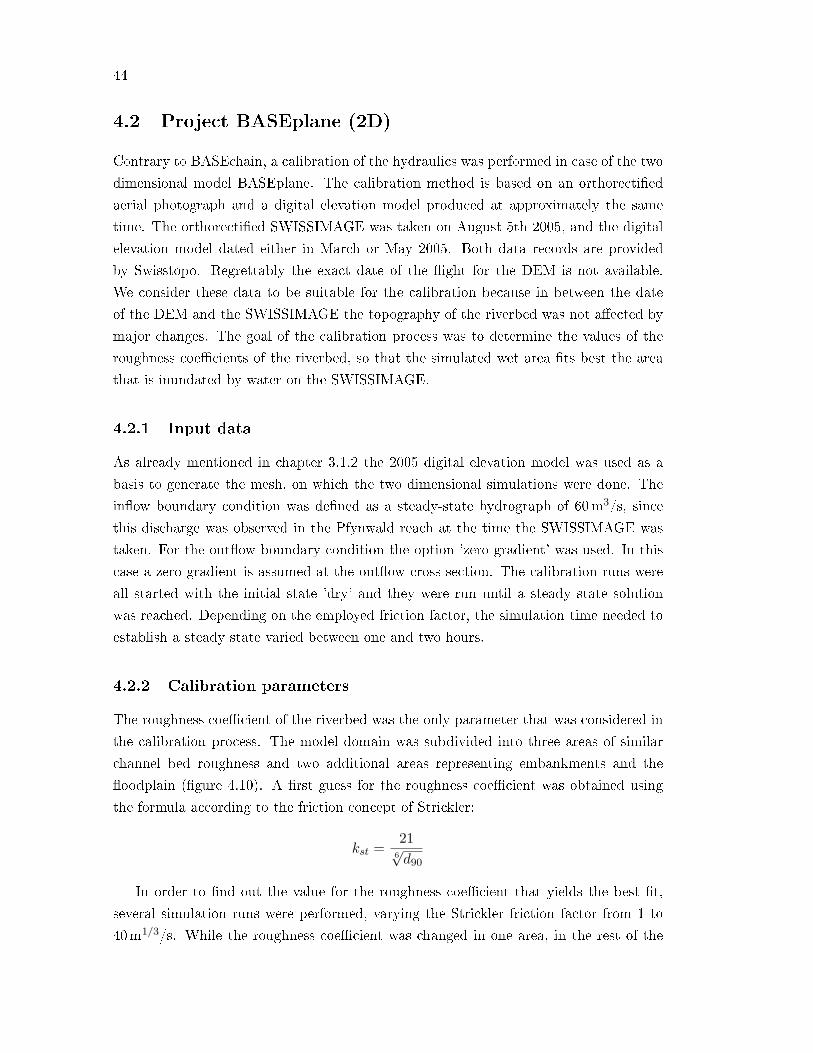
44
4.2 Project BASEplane (2D)
Contrary to BASEchain, a calibration of the hydraulics was performed in case of the two
dimensional model BASEplane. The calibration method is based on an orthorecti�ed
aerial photograph and a digital elevation model produced at approximately the same
time. The orthorecti�ed SWISSIMAGE was taken on August 5th 2005, and the digital
elevation model dated either in March or May 2005. Both data records are provided
by Swisstopo. Regrettably the exact date of the �ight for the DEM is not available.
We consider these data to be suitable for the calibration because in between the date
of the DEM and the SWISSIMAGE the topography of the riverbed was not a�ected by
major changes. The goal of the calibration process was to determine the values of the
roughness coe�cients of the riverbed, so that the simulated wet area �ts best the area
that is inundated by water on the SWISSIMAGE.
4.2.1 Input data
As already mentioned in chapter 3.1.2 the 2005 digital elevation model was used as a
basis to generate the mesh, on which the two dimensional simulations were done. The
in�ow boundary condition was de�ned as a steady-state hydrograph of 60m3/s, since
this discharge was observed in the Pfynwald reach at the time the SWISSIMAGE was
taken. For the out�ow boundary condition the option 'zero gradient' was used. In this
case a zero gradient is assumed at the out�ow cross section. The calibration runs were
all started with the initial state 'dry' and they were run until a steady state solution
was reached. Depending on the employed friction factor, the simulation time needed to
establish a steady state varied between one and two hours.
4.2.2 Calibration parameters
The roughness coe�cient of the riverbed was the only parameter that was considered in
the calibration process. The model domain was subdivided into three areas of similar
channel bed roughness and two additional areas representing embankments and the
�oodplain (�gure 4.10). A �rst guess for the roughness coe�cient was obtained using
the formula according to the friction concept of Strickler:
kst =21
6√d90
In order to �nd out the value for the roughness coe�cient that yields the best �t,
several simulation runs were performed, varying the Strickler friction factor from 1 to
40m1/3/s. While the roughness coe�cient was changed in one area, in the rest of the
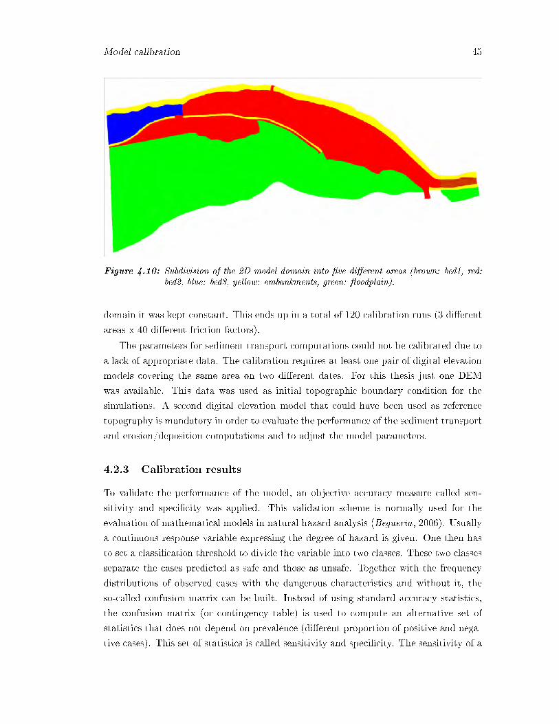
Model calibration 45
Figure 4.10: Subdivision of the 2D model domain into �ve di�erent areas (brown: bed1, red:bed2, blue: bed3, yellow: embankments, green: �oodplain).
domain it was kept constant. This ends up in a total of 120 calibration runs (3 di�erent
areas x 40 di�erent friction factors).
The parameters for sediment transport computations could not be calibrated due to
a lack of appropriate data. The calibration requires at least one pair of digital elevation
models covering the same area on two di�erent dates. For this thesis just one DEM
was available. This data was used as initial topographic boundary condition for the
simulations. A second digital elevation model that could have been used as reference
topography is mandatory in order to evaluate the performance of the sediment transport
and erosion/deposition computations and to adjust the model parameters.
4.2.3 Calibration results
To validate the performance of the model, an objective accuracy measure called sen-
sitivity and speci�city was applied. This validation scheme is normally used for the
evaluation of mathematical models in natural hazard analysis (Begueria, 2006). Usually
a continuous response variable expressing the degree of hazard is given. One then has
to set a classi�cation threshold to divide the variable into two classes. These two classes
separate the cases predicted as safe and those as unsafe. Together with the frequency
distributions of observed cases with the dangerous characteristics and without it, the
so-called confusion matrix can be built. Instead of using standard accuracy statistics,
the confusion matrix (or contingency table) is used to compute an alternative set of
statistics that does not depend on prevalence (di�erent proportion of positive and nega-
tive cases). This set of statistics is called sensitivity and speci�city. The sensitivity of a
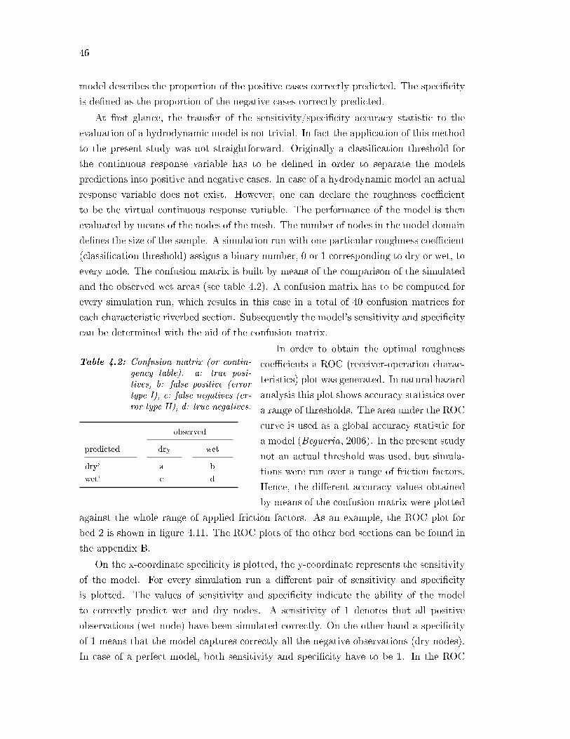
46
model describes the proportion of the positive cases correctly predicted. The speci�city
is de�ned as the proportion of the negative cases correctly predicted.
At �rst glance, the transfer of the sensitivity/speci�city accuracy statistic to the
evaluation of a hydrodynamic model is not trivial. In fact the application of this method
to the present study was not straightforward. Originally a classi�cation threshold for
the continuous response variable has to be de�ned in order to separate the models
predictions into positive and negative cases. In case of a hydrodynamic model an actual
response variable does not exist. However, one can declare the roughness coe�cient
to be the virtual continuous response variable. The performance of the model is then
evaluated by means of the nodes of the mesh. The number of nodes in the model domain
de�nes the size of the sample. A simulation run with one particular roughness coe�cient
(classi�cation threshold) assigns a binary number, 0 or 1 corresponding to dry or wet, to
every node. The confusion matrix is built by means of the comparison of the simulated
and the observed wet areas (see table 4.2). A confusion matrix has to be computed for
every simulation run, which results in this case in a total of 40 confusion matrices for
each characteristic riverbed section. Subsequently the model's sensitivity and speci�city
can be determined with the aid of the confusion matrix.
Table 4.2: Confusion matrix (or contin-gency table). a: true posi-tives, b: false positive (errortype I), c: false negatives (er-ror type II), d: true negatives.
observed
predicted dry wet
dry' a b
wet' c d
In order to obtain the optimal roughness
coe�cients a ROC (receiver-operation charac-
teristics) plot was generated. In natural hazard
analysis this plot shows accuracy statistics over
a range of thresholds. The area under the ROC
curve is used as a global accuracy statistic for
a model (Begueria, 2006). In the present study
not an actual threshold was used, but simula-
tions were run over a range of friction factors.
Hence, the di�erent accuracy values obtained
by means of the confusion matrix were plotted
against the whole range of applied friction factors. As an example, the ROC plot for
bed 2 is shown in �gure 4.11. The ROC plots of the other bed sections can be found in
the appendix B.
On the x-coordinate speci�city is plotted, the y-coordinate represents the sensitivity
of the model. For every simulation run a di�erent pair of sensitivity and speci�city
is plotted. The values of sensitivity and speci�city indicate the ability of the model
to correctly predict wet and dry nodes. A sensitivity of 1 denotes that all positive
observations (wet node) have been simulated correctly. On the other hand a speci�city
of 1 means that the model captures correctly all the negative observations (dry nodes).
In case of a perfect model, both sensitivity and speci�city have to be 1. In the ROC

Model calibration 47
0.75 0.8 0.85 0.9 0.95 10.75
0.8
0.85
0.9
0.95
1
specificity (true negative fraction)
se
nsitiv
ity (
tru
e p
ositiv
e fra
ctio
n)
Figure 4.11: Receiver-operation characteristics (ROC) plot at the example of bed 2.
plot the sensitivity/speci�city pair of a perfect model would be situated in the upper
right corner. Consequently a model performs well, the closer the corresponding pair of
sensitivity and speci�city lies to the upper right corner in a ROC plot.
To determine the roughness coe�cient for which the model performs best, an accu-
racy statistic T = sensitivity + speci�city is de�ned. Plotting this statistic as a function
of the roughness coe�cient allows us to objectively de�ne the best value for the friction
factor (�gure 4.12). The best model performance is achieved at the maximum value of
T. The values for the optimal as well as the computed Strickler roughness coe�cients
are summarized in table 4.3.
Table 4.3: Calibrated and computed roughness coe�cients.
bed 1 bed 2 bed 3
calibrated roughness coe�cient 33m1/3/s 11m1/3/s 12m1/3/s
roughness coe�cient according to d90 35m1/3/s 23m1/3/s 25m1/3/s
Using the Strickler formula to compute the friction factor on the basis of the charac-
teristic grain diameter d90, results in larger values. A large Strickler roughness coe�cient

48
corresponds to a smooth channel bed. This means that the Strickler formula underesti-
mates the roughness of the riverbed. The empirical formula according to Strickler just
takes into account the friction that is induced by the grains of the gravel bed. However
the total roughness of a channel bed consists not only of the grain friction, bedforms
also play a very important role, especially in case of a braided river. Bedforms such as
ri�es, dunes, antidunes and gravel banks cause additional friction losses. In case of the
Pfynwald reach the bedform fraction seems to be very high, decreasing the roughness
coe�cient of the channel bed for more than 10 Strickler units.
0 5 10 15 20 25 30 35 401.78
1.8
1.82
1.84
1.86
1.88
1.9
1.92
1.94
1.96
roughness coefficient kst
T =
su
m o
f se
nsitiv
ity a
nd
sp
ecific
ity
bed 1
bed 2
bed 3
Figure 4.12: Accuracy statistic T = sensitivity + speci�city.
Finally the best �t of the model for the whole domain is achieved by combining the
respective optimal friction factors of the three di�erent riverbed sections. The visual
result is illustrated in �gure 4.13. The graph shows the simulated water depth; in
the background the orthorecti�ed SWISSIMAGE from August 2005 is visible. This
combination allows a visual compromise of simulated wet areas and observed ones. At
this point is has to be mentioned again, that the DEM and the SWISSIMAGE are not
taken exactly at the same date, so that minor changes are ascribed to this circumstance.
The application of the sensitivity/speci�city accuracy measure highlights the excel-
lent performance of the model. The models sensitivity adds up to 0.93 and the speci�city
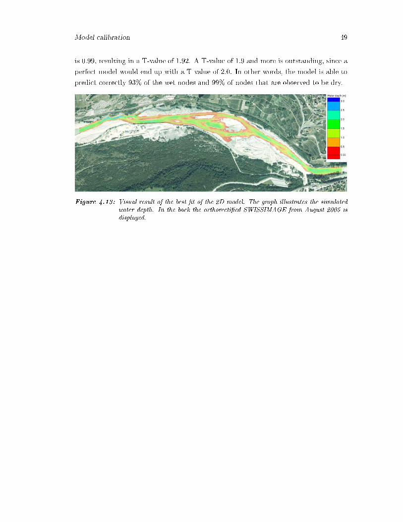
Model calibration 49
is 0.99, resulting in a T-value of 1.92. A T-value of 1.9 and more is outstanding, since a
perfect model would end up with a T-value of 2.0. In other words, the model is able to
predict correctly 93% of the wet nodes and 99% of nodes that are observed to be dry.
Figure 4.13: Visual result of the best �t of the 2D model. The graph illustrates the simulatedwater depth. In the back the orthorecti�ed SWISSIMAGE from August 2005 isdisplayed.

50
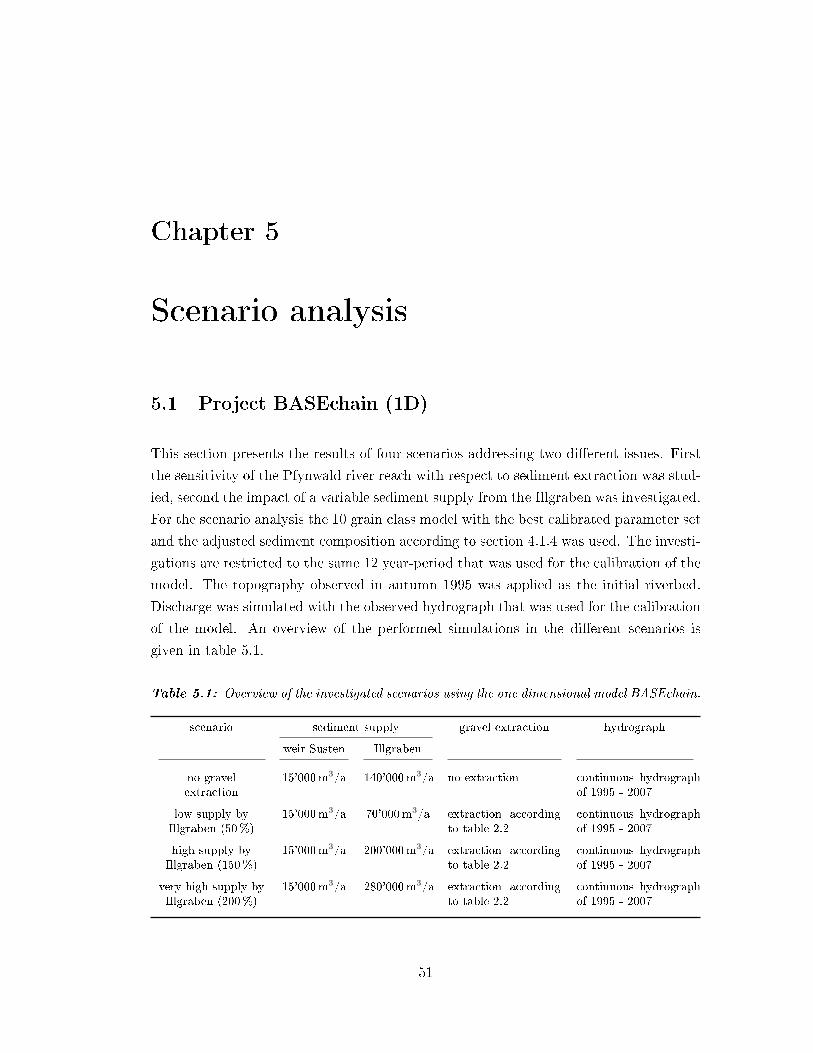
Chapter 5
Scenario analysis
5.1 Project BASEchain (1D)
This section presents the results of four scenarios addressing two di�erent issues. First
the sensitivity of the Pfynwald river reach with respect to sediment extraction was stud-
ied, second the impact of a variable sediment supply from the Illgraben was investigated.
For the scenario analysis the 10 grain class model with the best calibrated parameter set
and the adjusted sediment composition according to section 4.1.4 was used. The investi-
gations are restricted to the same 12 year-period that was used for the calibration of the
model. The topography observed in autumn 1995 was applied as the initial riverbed.
Discharge was simulated with the observed hydrograph that was used for the calibration
of the model. An overview of the performed simulations in the di�erent scenarios is
given in table 5.1.
Table 5.1: Overview of the investigated scenarios using the one dimensional model BASEchain.
scenario sediment supply gravel extraction hydrograph
weir Susten Illgraben
no gravelextraction
15'000m3/a 140'000m3/a no extraction continuous hydrographof 1995 - 2007
low supply byIllgraben (50%)
15'000m3/a 70'000m3/a extraction accordingto table 2.2
continuous hydrographof 1995 - 2007
high supply byIllgraben (150%)
15'000m3/a 200'000m3/a extraction accordingto table 2.2
continuous hydrographof 1995 - 2007
very high supply byIllgraben (200%)
15'000m3/a 280'000m3/a extraction accordingto table 2.2
continuous hydrographof 1995 - 2007
51
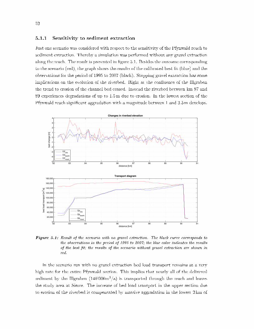
52
5.1.1 Sensitivity to sediment extraction
Just one scenario was considered with respect to the sensitivity of the Pfynwald reach to
sediment extraction. Thereby a simulation was performed without any gravel extraction
along the reach. The result is presented in �gure 5.1. Besides the outcome corresponding
to the scenario (red), the graph shows the results of the calibrated best �t (blue) and the
observations for the period of 1995 to 2007 (black). Stopping gravel extraction has some
implications on the evolution of the riverbed. Right at the con�uence of the Illgraben
the trend to erosion of the channel bed ceased. Instead the riverbed between km 87 and
89 experiences degradations of up to 1.5m due to erosion. In the lowest section of the
Pfynwald reach signi�cant aggradation with a magnitude between 1 and 3.5m develops.
82 83 84 85 86 87 88 89 90 91-5
-4
-3
-2
-1
0
1
2
3
4Changes in riverbed elevation
distance [km]
be
d c
ha
ng
e [m
]
DZobs
DZbestfit
DZnoext
82 83 84 85 86 87 88 89 90 910
20,000
40,000
60,000
80,000
100,000
120,000
140,000
160,000
180,000Transport diagram
distance [km]
be
d lo
ad
tra
nsp
ort
[m
3/a
]
Qbobs
Qbbestfit
Qbnoext
Figure 5.1: Result of the scenario with no gravel extraction. The black curve corresponds tothe observations in the period of 1995 to 2007; the blue color indicates the resultsof the best �t; the results of the scenario without gravel extraction are shown inred.
In the scenario run with no gravel extraction bed load transport remains at a very
high rate for the entire Pfynwald section. This implies that nearly all of the delivered
sediment by the Illgraben (140'000m3/a) is transported through the reach and leaves
the study area at Sierre. The increase of bed load transport in the upper section due
to erosion of the riverbed is compensated by massive aggradation in the lowest 2 km of
Scenario analysis 53
the reach. At the lower end of the Pfynwald reach a di�erence in bed load transport
of roughly 120'000m3/a results between the scenario with no extraction and the obser-
vations. This corresponds approximately to the annual mean sediment volume that is
extracted at the gravel pits (see table 4.1).
The overall good impression of the simulation results is compromised by some very
sharp peaks between km 84 and 86. These unnatural features are presumably induced
by numerical instabilities or inconsistencies in the model.
5.1.2 Sensitivity to sediment supply by the Illgraben
The sensitivity of the Pfynwald reach to a variable sediment supply by the Illgraben
was investigated by means of three di�erent simulation runs. Thereby the delivered
sediment by the Illgraben was assumed to amount to 70'000m3/a, 200'000m3/a respec-
tively 280'000m3/a corresponding to 50%, 150% and 200% of the actually observed
mean annual supply between 1995 and 2007. The simulated changes of the riverbed
elevation and the bed load transport rate are presented in �gure 5.2. Besides the three
scenario runs, the results of the calibrated best �t with a supply of 140'000m3/a as well
as the observations are plotted. In general no signi�cant di�erences can be observed
between the di�erent simulations, which implies that either the Pfynwald reach or even
more likely the model is not very sensitive to the supplied sediment. Not even a dou-
bling of the delivered debris �ow material causes aggradation in the Pfynwald reach.
The most signi�cant response is for a reduced supply of 70'000m3/a. Around km 89 the
model computes relatively large erosion of the channel bed.
The transport diagram points out that the sediment out�ow at the downstream
boundary of the Pfynwald reach is directly proportional to the delivered sediment volume
by the Illgraben.
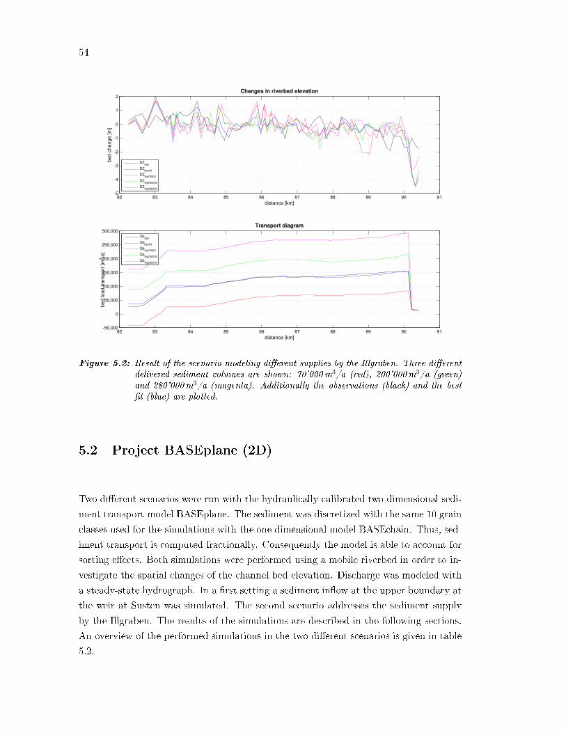
54
82 83 84 85 86 87 88 89 90 91-5
-4
-3
-2
-1
0
1
2Changes in riverbed elevation
distance [km]
be
d c
ha
ng
e [m
]
DZobs
DZbestfit
DZIllg70000
DZIllg200000
DZIllg280000
82 83 84 85 86 87 88 89 90 91-50,000
0
50,000
100,000
150,000
200,000
250,000
300,000Transport diagram
distance [km]
be
d lo
ad
tra
nsp
ort
[m
3/a
]
Qb
obs
Qbbestfit
QbIllg70000
QbIllg200000
QbIllg280000
Figure 5.2: Result of the scenario modeling di�erent supplies by the Illgraben. Three di�erentdelivered sediment volumes are shown: 70'000m3/a (red), 200'000m3/a (green)and 280'000m3/a (magenta). Additionally the observations (black) and the best�t (blue) are plotted.
5.2 Project BASEplane (2D)
Two di�erent scenarios were run with the hydraulically calibrated two dimensional sedi-
ment transport model BASEplane. The sediment was discretized with the same 10 grain
classes used for the simulations with the one dimensional model BASEchain. Thus, sed-
iment transport is computed fractionally. Consequently the model is able to account for
sorting e�ects. Both simulations were performed using a mobile riverbed in order to in-
vestigate the spatial changes of the channel bed elevation. Discharge was modeled with
a steady-state hydrograph. In a �rst setting a sediment in�ow at the upper boundary at
the weir at Susten was simulated. The second scenario addresses the sediment supply
by the Illgraben. The results of the simulations are described in the following sections.
An overview of the performed simulations in the two di�erent scenarios is given in table
5.2.

Scenario analysis 55
Table 5.2: Overview of the investigated scenarios using the two dimensional model BASEplane.
scenario sediment supply gravel extraction hydrograph
weir Susten Illgraben
sediment boundarycondition
0,1m3/s no input no extraction steady-state hydro-graph of 400m3/s
debris �ow event no input 25'000m3/h no extraction steady-state hydro-graph of 400m3/s
5.2.1 Simulation of the sediment in�ow at the upper boundary condi-
tion
In case of a �ood in the Rhone, bed load passes the weir at Susten and enters the
Pfynwald reach. This section is dedicated to the simulation of this scenario. Thereby the
delivered sediment from upstream is inserted into the model domain as upper boundary
condition. A steady-state sediment �ux of 0.1m3/s was taken to represent the bed load
in�ow. The simulation was run for one hour, so that a total of 360m3 of sediment
entered the model domain. The constitution of the supplied material was modeled with
a mean particle diameter of 60mm. Discharge was simulated by means of a steady-state
�ow rate of 400m3/s. The de�nition of the initial condition was done with the aid of an
old hydraulic simulation.
Figure 5.3 shows the simulated changes of the riverbed. Erosion is indicated with
blue colors; aggradation is shown with yellow to brown colors. The magnitude of the
channel bed changes ranges from erosion in the order of 1m to deposition up to 2m. Two
main sections of riverbed changes can be identi�ed. On the one hand the area right at the
con�uence of the Illgraben is a�ected by major erosion of the channel bed. Thereafter
a section of alternating erosion and aggradation follows. On the other hand there are
signi�cant riverbed changes in the lowest part of the study area. The observed pattern of
erosion and deposition reminds one strongly of an alternating bar morphology. Right at
the beginning of the model domain the model computes locally large aggradation, which
is adjacent to a node with signi�cant erosion. This phenomenon is certainly related
to the de�nition of the sediment in�ow boundary condition. Surprisingly no riverbed
changes are simulated in the central part of the study area.
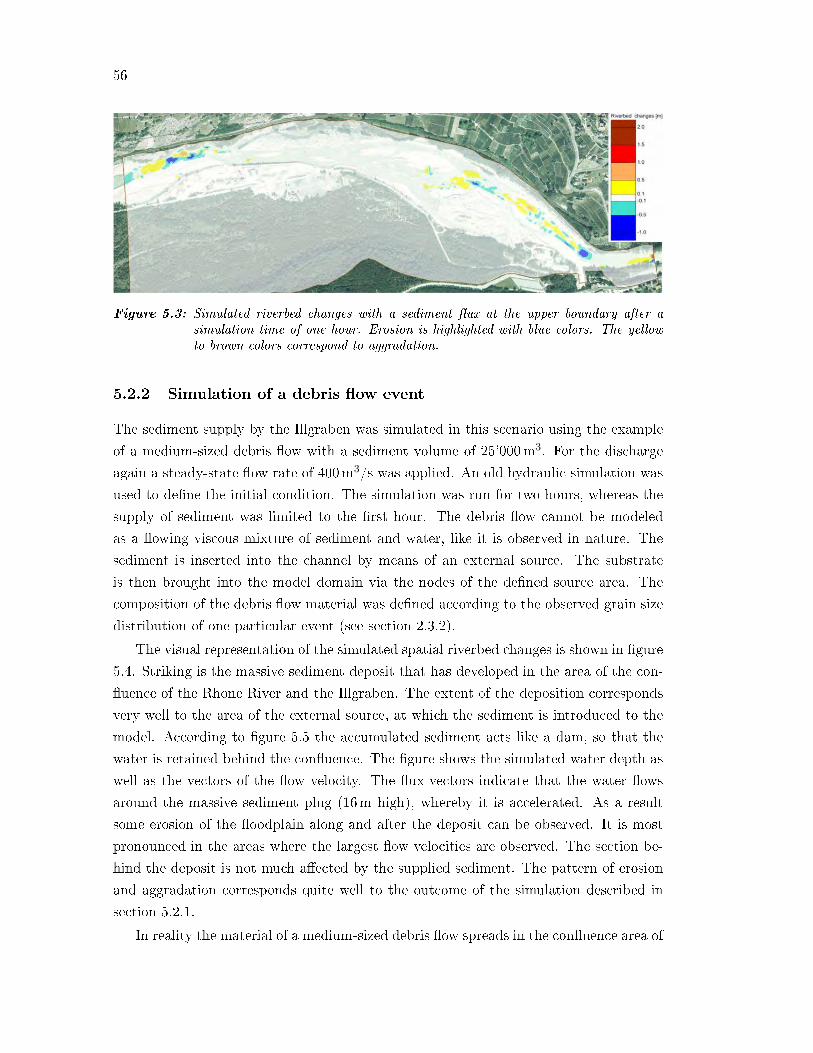
56
Figure 5.3: Simulated riverbed changes with a sediment �ux at the upper boundary after asimulation time of one hour. Erosion is highlighted with blue colors. The yellowto brown colors correspond to aggradation.
5.2.2 Simulation of a debris �ow event
The sediment supply by the Illgraben was simulated in this scenario using the example
of a medium-sized debris �ow with a sediment volume of 25'000m3. For the discharge
again a steady-state �ow rate of 400m3/s was applied. An old hydraulic simulation was
used to de�ne the initial condition. The simulation was run for two hours, whereas the
supply of sediment was limited to the �rst hour. The debris �ow cannot be modeled
as a �owing viscous mixture of sediment and water, like it is observed in nature. The
sediment is inserted into the channel by means of an external source. The substrate
is then brought into the model domain via the nodes of the de�ned source area. The
composition of the debris �ow material was de�ned according to the observed grain size
distribution of one particular event (see section 2.3.2).
The visual representation of the simulated spatial riverbed changes is shown in �gure
5.4. Striking is the massive sediment deposit that has developed in the area of the con-
�uence of the Rhone River and the Illgraben. The extent of the deposition corresponds
very well to the area of the external source, at which the sediment is introduced to the
model. According to �gure 5.5 the accumulated sediment acts like a dam, so that the
water is retained behind the con�uence. The �gure shows the simulated water depth as
well as the vectors of the �ow velocity. The �ux-vectors indicate that the water �ows
around the massive sediment plug (16m high), whereby it is accelerated. As a result
some erosion of the �oodplain along and after the deposit can be observed. It is most
pronounced in the areas where the largest �ow velocities are observed. The section be-
hind the deposit is not much a�ected by the supplied sediment. The pattern of erosion
and aggradation corresponds quite well to the outcome of the simulation described in
section 5.2.1.
In reality the material of a medium-sized debris �ow spreads in the con�uence area of
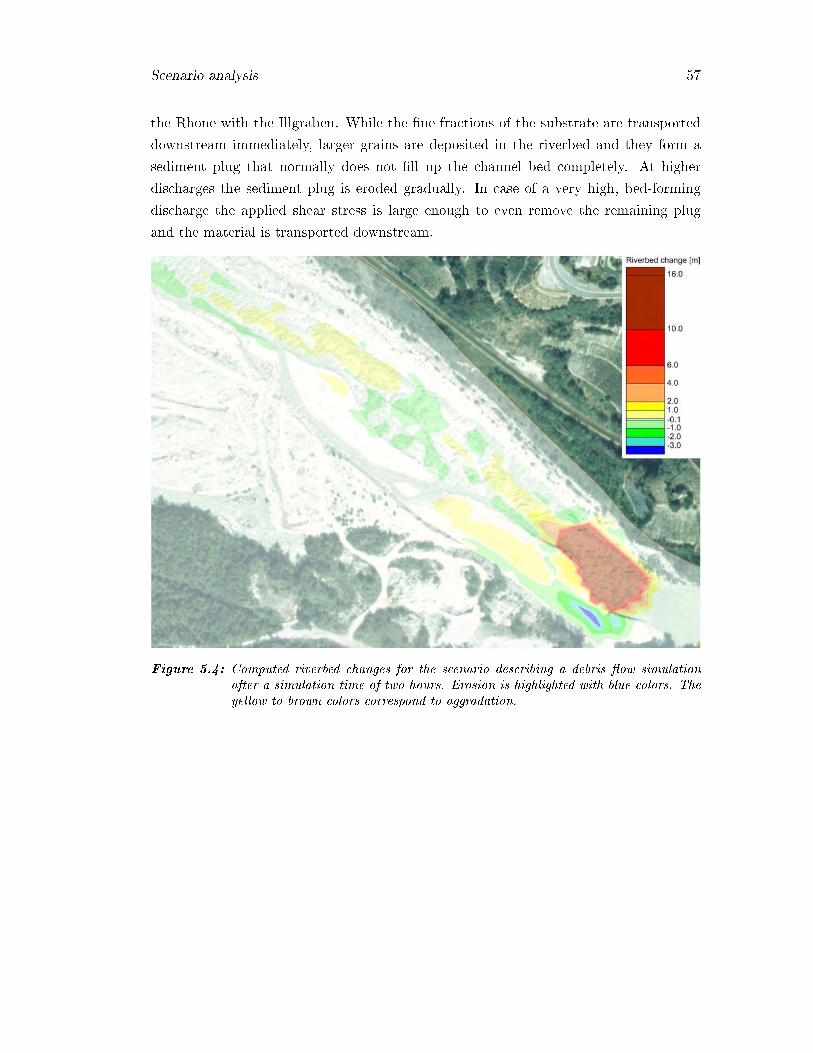
Scenario analysis 57
the Rhone with the Illgraben. While the �ne fractions of the substrate are transported
downstream immediately, larger grains are deposited in the riverbed and they form a
sediment plug that normally does not �ll up the channel bed completely. At higher
discharges the sediment plug is eroded gradually. In case of a very high, bed-forming
discharge the applied shear stress is large enough to even remove the remaining plug
and the material is transported downstream.
Figure 5.4: Computed riverbed changes for the scenario describing a debris �ow simulationafter a simulation time of two hours. Erosion is highlighted with blue colors. Theyellow to brown colors correspond to aggradation.
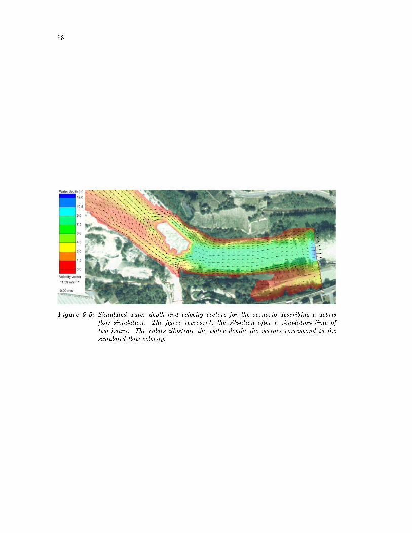
58
Figure 5.5: Simulated water depth and velocity vectors for the scenario describing a debris�ow simulation. The �gure represents the situation after a simulation time oftwo hours. The colors illustrate the water depth; the vectors correspond to thesimulated �ow velocity.
Chapter 6
Discussion
Right from the start it was clear that the application of a numerical model to the
Pfynwald reach is a very challenging task. The braided morphology of the Rhone, the
steepness and the large variability in the width of the riverbed, the frequent hydraulic
drops and the massive sediment input through the debris �ows in the Illgraben are some
of the exceptional characteristics of this river reach, which complicate the successful
use of numerical models. This fact has been approved explicitly by the investigations of
Hunziker, Zarn & Partner AG (2001). Although the development of computer programs
as well as the scienti�c research in the �eld of sediment transport was advanced since
then, morphodynamic modeling of such systems remains a challenging task. For this
thesis the software system BASEMENT was used. According to the developers one
main focus of this system is the stability of the numerical models. Further it was
designed explicitly for the simulation of alpine rivers and sediment transport. However,
the application of BASEMENT in the present study to the alpine Pfynwald river reach
reveals several problems. In the next sections these di�culties are discussed in detail.
6.1 Project BASEchain (1D)
6.1.1 Model calibration
On the contrary to the study of Hunziker, Zarn & Partner AG (2001) the frequent
hydraulic drops did fortunately not create numerical instabilities in the present hydraulic
computations. Generally the one dimensional model BASEchain performed well in case
of pure hydraulic simulations (see also �gure 4.2). A proper calibration of the hydraulic
model was not conducted due to the lack of data that would have been needed for
it. Additionally the improvement of the sediment transport computations is negligible
compared to the e�ect of a calibration of the sediment transport parameters. Therefore
in this study I focused on the identi�cation of important calibration parameters related
59
60
to sediment transport. The sensitivity of di�erent model parameters to the output
was the main focus (see chapter 4.1). Obviously the goal was to identify the most
sensitive parameters in order to adjust as many parameters as necessary to obtain the
best �t. In principle the sensitivity analysis of the model parameters was thought to
provide the best parameter con�guration for the subsequent scenario analysis. Shortly
after the start of the calibration of BASEchain serious problems appeared, so that the
calibration process was delayed. The model su�ered from several bugs. At the beginning
BASEchain was not able at all to run a simulation without crashing due to numerical
instabilities. The developers of BASEMENT at VAW were then contacted in order to
remove bugs in the model code. After solving a couple of bugs in the code the simulation
results signi�cantly improved. Especially the occurrence of numerical instabilities could
be reduced tremendously. Finally, the calibration and the adjustment of BASEchain to
the study reach became a very time consuming component of this thesis and eclipsed
the actual planned scenario analysis.
In the scope of the calibration of the model, the most important parameters could
be identi�ed. Clearly the most crucial of all the calibration parameters is the upwind
parameter, which determines the interpolation of bed load �ux to the cell interface. An
inappropriate value provokes numerical instabilities leading to unfeasible simulation re-
sults. For that reason it is advisable to �nd out the most suitable value for the upwind
parameter before calibrating the rest of the parameters. A less important calibration pa-
rameter is the active layer height. It does have signi�cant e�ects regarding the bed load
transport rate and the occurrence of numerical instabilities. In this study the reduction
of the active layer height generally attenuated the occurrence and the magnitude of nu-
merical instabilities. Thus, the parameter can be used to reduce or even avoid numerical
instabilities on a small scale. Concerning bed load transport, the expected increase of
bed load transport using a larger active layer height was only partially con�rmed. The
modeling results are too inconsistent in order to make a general statement about the
relationship between the active layer height and the computed sediment transport rate.
Sediment transport models should be calibrated on long periods in order to avoid
e�ects of short- to medium-term process variability. In the present study the model
is calibrated on the basis of a period that spans 12 years. This length corresponds
to a medium temporal scale. Consequently the model may be inappropriate for the
simulation of short-term processes like for example the change in the riverbed during an
individual �ood event.
Discussion 61
Number of grain classes
The number of grain classes that discretize the sediment grain size distribution is a
very important calibration parameter. It determines if fractional sediment transport
can be applied and thus sorting e�ects can be modeled. The calibration results show
that a single grain simulation is not able to simulate satisfactorily sediment transport in
the Pfynwald reach. In general too little sediment transport is computed, which leads
to the development of large aggradation. An increase in the number of grain classes
produces an increase in the bed load transport capacity in the Pfynwald river reach.
To explain this behavior one needs to take into account the unique setting in this river
reach. Sediment transport usually takes place when the shear stress applied by the �ow
exceeds the bed shear stress of the riverbed, so that the armored layer is broken up. This
happens only at very high, so-called bed forming discharges. In this case a sediment
transport simulation is not very sensitive to the applied number of grain classes, because
the induced stress by the �ow is large enough to mobilize the whole spectrum of grain
sizes. Sorting e�ects are negligible, so that fractional sediment transport is not required
explicitly. In this case a single grain simulation would be su�cient.
In the Pfynwald reach sediment transport takes place not only at the breakup of the
armored layer, but also in case of a debris �ow in the Illgraben. These debris �ows occur
even during low �ows in the Rhone River, when the �ow is just able to transport the �ne
fractions of the supplied debris �ow material. Therefore fractional sediment transport
is very important in order to be able to simulate correctly the ongoing processes. To
compute the mean grain size of a grain class, the average of the particle sizes in the
corresponding class, weighted by mass, is taken. A coarse resolution of the debris �ow
substrate cannot reproduce adequately the �ne sediment fractions, because in case of
only a few grain classes the range of grain sizes in one particular grain class is large,
so that �ne sediment fractions are averaged out. The larger the mean diameter of the
smallest grain class is, the less likely the �ow is able to transport this grain fraction
during low �ows. In other words, the more grain classes one takes into account, the
better the whole spectrum of di�erent grain sizes of a substrate can be represented and
the more grain classes are transported by the �ow even during low �ows.
At this point the modi�cation of the applied hydrograph should be mentioned. The
negligence of discharges below 100m3/s has certainly an implication to the computation
of sediment transport in the Pfynwald reach. As already mentioned above, not the break-
up of the armored layer is crucial in terms of sediment transport but the occurrence
of debris �ows. A model with a clipped hydrograph cannot account for the ongoing
processes during a debris �ow that enters the Rhone at a discharge below the considered
minimum stream�ow.
62
In the model the sediment supply by the Illgraben is simulated as constant in�ow,
independently of the observed discharge in the Rhone River. In order to simulate sat-
isfactorily sediment transport in the Pfynwald reach it is indispensable to employ frac-
tional sediment transport. Moreover it is important to use a su�cient amount of grain
classes to discretize the sediment. But it does not make sense to consider more grain
classes than needed for the sake of the computational e�ciency. Besides, the chance
to encounter numerical instabilities increases with a larger number of considered grain
classes as it was observed in the calibration process. In the present study the use of
10 grain classes seems to be adequate in order to obtain satisfying results and to avoid
major numerical instabilities.
Apart from the insu�cient modeling of sediment transport due to the missing com-
putation of sorting e�ects, the single grain simulation exposes an inconsistency relating
to the calculation of sediment relocation. The problem is manifested best at the example
of the fact that bed load transport drops to negative values approaching the lower end
of the river section. In nature this can de�nitely not happen, because it implies that
the model extracts or deposits sediment that is actually not available. Consequently the
model does not allow for mass conservation.
To locate the error in the model code for the computation of sediment relocation, a
simulation run was performed modeling just the sediment extraction. Thereby a �xed
riverbed was applied in order to not disturb the evolution of the riverbed by sedimenta-
tion and erosion processes. Sediment relocation was then tested based on the comparison
of the simulated erosion caused by the sediment extraction and the corresponding bed
load transport. If sediment relocation is computed correctly the simulated erosion has to
compensate the extraction volumes. Because there is no additional sediment input, nei-
ther a supply by the Illgraben nor an input at the upper boundary the resulting bed load
transport is zero. Figure 6.1 illustrates the result of a simulation run to test BASEchains
algorithm to compute sediment relocation. The transport diagram supports explicitly
the above denoted concerns regarding the computation of sediment relocation, since the
simulated erosion does not correspond to the actual extracted sediment volume. The
blue curve highlights bed load transport considering the eroded sediment volume. The
red line does not account for erosion. Thus, the di�erence between the two curves corre-
sponds to the simulated eroded sediment volume. As a consequence of this, BASEchain
consistently computes too little erosion at the location of external sinks. The mass bal-
ance error in the computed eroded sediment volume is indicated by the green curve.
On average, the mass balance error adds up to -75%, which implies that 75% of the
extracted sediment volume is not converted into channel bed erosion.
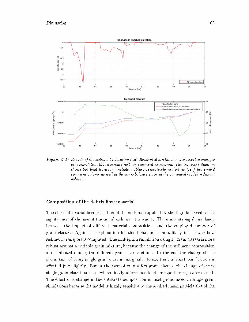
Discussion 63
82 83 84 85 86 87 88 89 90 91-4
-3.5
-3
-2.5
-2
-1.5
-1
-0.5
0Changes in riverbed elevation
distance [km]
be
d c
ha
ng
e [m
]
82 83 84 85 86 87 88 89 90 91-150,000
-100,000
-50,000
0
50,000Transport diagram
be
d lo
ad
tra
nsp
ort
[m
3/a
]
distance [km]
82 83 84 85 86 87 88 89 90 91-90
-85
-80
-75
-70
ma
ss b
ala
nce
err
or
[%]
DZ extraction alone
Qb extraction alone
Qb extraction alone, no extraction
Mass balance error in eroded sediment volume
Figure 6.1: Results of the sediment relocation test. Illustrated are the modeled riverbed changesof a simulation that accounts just for sediment extraction. The transport diagramshows bed load transport including (blue) respectively neglecting (red) the erodedsediment volume as well as the mass balance error in the computed eroded sedimentvolume.
Composition of the debris �ow material
The e�ect of a variable constitution of the material supplied by the Illgraben veri�es the
signi�cance of the use of fractional sediment transport. There is a strong dependency
between the impact of di�erent material compositions and the employed number of
grain classes. Again the explanation for this behavior is most likely in the way how
sediment transport is computed. The multigrain simulation using 10 grain classes is more
robust against a variable grain mixture, because the change of the sediment composition
is distributed among the di�erent grain size fractions. In the end the change of the
proportion of every single grain class is marginal. Hence, the transport per fraction is
a�ected just slightly. But in the case of only a few grain classes, the change of every
single grain class increases, which �nally a�ects bed load transport to a greater extent.
The e�ect of a change in the substrate composition is most pronounced in single grain
simulations because the model is highly sensitive to the applied mean particle size of the

64
sediment (see �gure 4.5).
In case of the 5 grain class simulations the riverbed elevation changes at the con-
�uence of the Illgraben do not a�ect the lowest part of the Pfynwald reach. Generally
�uvial systems are coupled in lateral as well as longitudinal direction, so that a local
change of the channel bed elevation can have major impacts on the whole river section.
This �nding implies the surprising fact that there is no signi�cant longitudinal coupling
of the channel bed in the 5 grain class model. In relation to that the results of the 10
grain class simulations appear to be more realistic, since the entire Rhone River reach is
a�ected by changes of the debris �ow substrate. A longitudinal coupling seems to exist,
because di�erent changes in the riverbed elevation at the beginning of the considered
river section provoke di�erent responses at the lower end of the Pfynwald reach.
Best �t
After a very extensive and cumbersome calibration of the one dimensional model BASE-
chain, �nally a model con�guration was found, which was able to simulate reasonably
well the observed riverbed changes and the mean annual bed load transport rate. Gen-
erally speaking the magnitude of the deviations from the observations lies in a tolerable
range. Just like all the calibration runs, the best �t simulation shows major erosion at
the beginning of the reach. This is most likely an e�ect of the de�nition of the upper
boundary condition. The de�nition of the boundary condition might also a�ect the
simulation results at the lower end of the Pfynwald reach between km 82 and 84 where
aggradation was simulated.
To evaluate the development of the riverbed elevation in the Pfynwald reach one
has to consider that the supply of the debris �ow material in the model is simulated as
a steady-state external source throughout the year. In reality the sediment, which is
supplied by the Illgraben, is delivered intermittently to the channel bed of the Rhone
River in only a few very large sediment inputs. In the majority of cases the discharge
in the Rhone is not able to carry away the delivered sediment all at once, so that a
gravel plug is formed in the con�uence area. The deposited material remains in the
channel bed of the Rhone until a �ood removes and carries it further downstream where
it is deposited again. This results in an intermittent transport of the debris �ow inputs
through the Pfynwald reach. The wave-like propagation of the aggradation leads to a
permanent pulsation of the riverbed, whose intensity is damped with increasing distance
to the Illgraben con�uence. This is highlighted very nicely in the plot of the temporal
evolution of the riverbed elevation (�gure 4.9). Jäggi (1988) describes this behavior in
detail in his extensive study about the Pfynwald reach. He also tried to estimate the
magnitude of the pulsation of the riverbed.
Discussion 65
A sediment transport model, which uses a simpli�ed continuous sediment supply
of the debris �ow material is certainly not able to simulate this short- to medium-
term pulsation of the riverbed as the plot of the temporal evolution of the channel bed
clearly indicates. For that reason the local discrepancy between the simulated and the
observed riverbed elevation change between km 87 and 88 might be explained with the
inability of the model to capture the pulsation of the riverbed. Though, the �gure of
the temporal channel bed change also shows that the model can capture the long-term
trend of the riverbeds development. Therefore the use of a continuous sediment supply
seems to be adequate in order to simulate the evolution of the longitudinal pro�le in the
Pfynwald river reach on a longer temporal scale. This is obvious, since the adjustment
of the riverbed on longer time scales is not a�ected by short-term processes, but more
importantly by characteristic mean boundary conditions and �uxes.
6.1.2 Scenario analysis
One speci�c goal of this thesis was to study the sensitivity of the Pfynwald reach to vari-
able boundary conditions. Originally it was planned to de�ne several scenarios, which
were characterized by di�erent boundary conditions. Due to the laborious calibration
of BASEchain, just a few of these simulation runs could be performed. The main focus
was set to the e�ect of a change of sediment extraction and the in�uence of a variable
sediment supply by the Illgraben.
Sensitivity to sediment extraction
The results of the simulation without gravel extraction demonstrate that the Rhone
River is on the average able to transport the delivered sediment by the Illgraben through
the Pfynwald river reach. In the long run, aggradation only occurs in the lowest part
of the Pfynwald reach that is characterized by a small channel bed gradient. As a
consequence not all of the currently existing gravel pits are required in order to prevent
the Pfynwald reach from signi�cant deposition caused by the large sediment inputs by
the Illgraben. However, the large volume of sediment that is carried out of the Pfynwald
section certainly has a major impact to the adjacent river section downstream of Sierre.
Since the slope of the longitudinal pro�le further decreases, the consequence is most
likely associated with large aggradation in this river section as this is already indicated
by the massive aggradation computed for the �at end of the Pfynwald reach. In order
to avoid negative impacts to the downstream river sections, it is therefore necessary to
continue to extract sediment in the Pfynwald reach. The extraction volume should be
determined by the transport capacity of the downstream river section.
The gravel extraction in the Pfynwald reach is an issue that is very much disputed.
66
Environmental organizations would like to stop the gravel extraction in order to estab-
lish a natural �uvial system that is completely una�ected by human interventions. As
a result an expertise was commissioned by the Canton Valais (Jäggi , 1988; Bezzola,
1989) to investigate the feasibility of a restoration of the natural river dynamics. The
study concludes that gravel extraction is required in order to guarantee su�cient �ood
protection for the surrounding areas.
In the scope of the sediment transport study of Hunziker, Zarn & Partner AG (2001)
the sensitivity of the Pfynwald reach to gravel extraction was also addressed. They ran a
scenario without any extraction. The sediment supply by the Illgraben was assumed to
be 100'000m3/a. A volume of 22'000 3/a was applied to the sediment in�ow at the upper
boundary. The simulation was run for a period of 26 years. The results and �ndings are
comparable to those obtained in the present thesis. In the uppermost 2 km of the reach
the model computes signi�cant erosion, while in the lower section a trend to relatively
large aggradation results. Regarding bed load transport a similar output was obtained
as well, concluding that the sediment discharge at the lower end of the reach corresponds
to the volume that is supplied by the debris �ows. Analog to the simulations in this
thesis the Rhone is able to transport the supplied volume of the debris �ows through
the Pfynwald reach. One needs to keep in mind that the model used by Hunziker was
calibrated on the basis of just four years.
With regard to sediment extraction, the way in which it is applied in the model as well
as in reality needs to be emphasized. In the Pfynwald reach gravel is extracted mainly
at three di�erent gravel pits. The extraction is restricted to the low �ow period during
winter, because in this time the riverbed can be accessed safely by heavy machinery.
In case of the model sediment extraction is modeled with spatially distributed sinks,
which allows representing the location of the extraction quite accurately. But the timing
of the extraction is not well represented, since the low �ow periods are not modeled.
Gravel extraction is simulated only for high discharges (Q>100m3/s) with a constant
extraction rate. In the model the processes of gravel extraction and sediment transport
interfere with each other as opposed to reality. This may have some implications to
the evolution of the riverbed, since the complex feedback mechanism behind sediment
transport and channel bed changes might be disturbed by simultaneous gravel extraction
in the model.
Sensitivity to sediment supply by the Illgraben
According to the results of the simulation runs with variable sediment supply by the
Illgraben, the Pfynwald reach is not sensitive to the volume of the material input. This
result is very surprising, because it is contrary to what one would actually expect based
Discussion 67
on the physical understanding of sediment transport in a river. In the same way Hun-
ziker, Zarn & Partner AG (2001) tested the sensitivity of the Pfynwald reach to sediment
supply with the aid of a numerical sediment transport model. Their results are contra-
dictory to the �nding in this thesis. They conclude that an increase of the sediment
input by the Illgraben causes major aggradation in the Pfynwald reach. By contrast a
decreased supply results in signi�cant erosion. For that reason the result in this thesis
is doubtful and we cannot make the statement that the Pfynwald reach is e�ectively
non-sensitive to the volume of the supplied sediment. One rather concludes that the
applied sediment transport model is not sensitive to the sediment input and it may not
be suitable to investigate this particular attribute of the river reach.
A possible explanation for the lack of response to a variable sediment supply by the
Illgraben may be the continuous implementation of the debris �ow input. The use of
episodic inputs, as it would be in reality may generate more aggradation in the channel
bed close to the con�uence.
6.1.3 Limitations of the model
The troubles that have emerged during the calibration of BASEchain as well as the di�-
culties that have been experienced in a previous study (Hunziker, Zarn & Partner AG ,
2001) raise the concern if a one dimensional model is actually appropriate to simulate
sediment transport in the Pfynwald river reach. As a result of the braided morphology,
the Rhone River has a two dimensional character in the area of the Pfynwald. Very of-
ten the water is �owing in di�erent river branches, which are not always parallel to the
main direction of the riverbed. In addition, the �ow frequently changes from subcritical
to supercritical �ow due to the irregular and partly quite steep channel bed. For that
reason the assumptions behind a one dimensional model may not be valid anymore for
parts or even the complete study area, so that the simpli�cations in the mathematical
model can lead to inconsistencies and errors in the simulation results. In consideration
of the di�culties which BASEchain encountered and the two dimensional character of
the Pfynwald reach, it is legitimate to ask if a two dimensional sediment transport model
should be more applicable to the Pfynwald river reach. 2d models are able not only to
simulate lateral �ow but also to provide spatial changes of the riverbed. However, a
huge drawback of two dimensional simulations is certainly the much longer computation
time. It is often not feasible to apply a two dimensional model for the analysis of the
evolution of the longitudinal pro�le or for the study of the sediment balance in a river
section.
Particularly in the very unique Pfynwald river reach, one may also doubt the applica-
bility of the concepts that are incorporated in the numerical sediment transport models

68
in general. The scope of application of the sediment transport formulas is limited. The
most widely-used formulas are practically all deduced from measurements in laboratory
experiments and they are based on the concept of complete mobility, meaning that all
fractions of the sediment substrate are in motion. In order to account for sorting ef-
fects, correction functions were deduced for fractional sediment transport in numerical
models (Hunziker , 1995). The prevailing circumstances in the Pfynwald section are cer-
tainly at the limits of the operative range of the sediment transport formulas. Mainly
the relatively large fraction of huge grain sizes (> 0.5m) is a problem in terms of the
computation of incipient motion and resulting sediment transport.
In this context it has to be mentioned that BASEchain does not provide a sediment
transport formula speci�cally developed for the special conditions in braided rivers. Such
formulas were developed for example by Zarn (1997) and Marti (2006). They account
for gravel banks and separate channels in a braided river by means of a mean water level
width and depth and a correction factor for slope.
A further limitation of the model concerns abrasion of sediment particles, meaning
that the decrease of the characteristic mean particle diameter of the riverbed substrate
along a river by the processes of e.g. splitting is not considered in the model.
Finally a remark about the de�nition of the initial conditions is given. BASEchain
allows for the de�nition of the hydraulic initial conditions, but it does not provide the
de�nition of an initial condition concerning the composition of the riverbed. Therefore
one cannot start a simulation with an already existing armored layer. The model has
to compute it �rst, so that the beginning of a simulation run is always a�ected by the
sorting processes leading to the formation of an armored layer.
6.2 Project BASEplane (2D)
6.2.1 Model calibration
The two dimensional project used a di�erent approach to calibrate the model. The main
work consisted of the calibration of the hydraulic model. Since the roughness coe�cient
is the only parameter that is worth to calibrate, the calibration process is relatively
simple. There is no interaction of di�erent parameters or any feedback mechanism that
need to be taken into account. The critical point in the calibration process is the evalua-
tion of the calibration results. A small change of the roughness coe�cient produces just
a minor di�erence in the model output. Therefore it is rather di�cult to identify the
optimal value of the friction factor at �rst sight. Besides, a qualitative judgment of an
output plot is always a�ected by the personal subjective impression. In order to guar-
antee an objective evaluation of the models performance sensitivity/speci�city accuracy
Discussion 69
measures were applied (Begueria, 2006). Although this method was actually designed
for the evaluation of mathematical models in natural hazard analysis, it has been proven
in this study that it is also suitable to quantitatively estimate the performance of a two
dimensional hydrodynamic model. A great advantage of the sensitivity/speci�city ap-
proach is the robustness with respect to unequal sample sizes. The number of dry and
wet nodes in the model domain is usually not equal and it strongly depends on the
de�nition and the characteristics of the model domain (e.g. �oodplain, embankments,
channel width) as well as on the simulated discharge (e.g. low �ows, �oods). In order
to guarantee a consistent evaluation of the model results e.g. over the range of di�erent
discharges it is very important to have an accuracy measure that is able to deal with
the presence of prevalence.
The successful calibration of a two dimensional hydrodynamic model makes high
demands on the availability of compatible data. The calibration requires pairs of aerial
photos and digital elevation models that were recorded at the same time. If one relies on
the data from Swisstopo it is only by chance that an aerial image matches the available
digital elevation model. Unfortunately the publicly available aerial photos and the digital
elevation model data are not recorded on the same �ights at Swisstopo, so that there
is always a temporal gap between the two datasets. The data availability tremendously
increases if a river section is permanently monitored e.g. in the scope of a research
project. A good example is the RECORD project at the Thur River (RECORD , 2010).
The calibration of the two dimensional hydrodynamic model in this study was based
just on one pair of an aerial picture and a digital elevation model for the Pfynwald
reach. That is su�cient data simply for one calibration scenario, for a discharge of
60m3/s which was measured at the time the aerial picture was taken. This �ow rate
corresponds approximately to the mean hourly discharge that was observed in the period
of 1974 to 2008. Preferably a hydrodynamic model should be calibrated for a range of
di�erent �ow rates, because the total roughness of a riverbed is not constant. Depending
on discharge, the friction that is induced to the �ow by the riverbed is changing. Most
pronounced is the �ow rate dependent roughness in the case of bedform induced friction.
While during low �ows gravel banks remain dry and do not a�ect stream�ow, they can
add signi�cantly to total roughness if they are inundated in case of high �ows.
Concerning riverbed roughness it is also worth to look at the values of the calibrated
roughness coe�cient. In particular the comparison of the initial values obtained by
means of the characteristic grain size d90 and the calibrated values is very interesting
and shows that a signi�cant fraction of the total roughness of a braided riverbed consists
of roughness induced by bedforms.
Finally the excellent performance of the hydrodynamic part of BASEplane should
be mentioned. Using the calibrated parameter set, the model simulates very well the
70
hydraulics of the Pfynwald reach. The good performance of BASEplane in the Pfynwald
reach allows for the conclusion that the model is certainly quali�ed for the hydraulic
simulation of alpine rivers, even if they exhibit a very complex topography.
6.2.2 Scenario analysis
The main focus of the simulations with the two dimensional model BASEplane was to
test the ability of the model to simulate sediment transport in the Pfynwald reach using
a mobile riverbed as well as the investigation of spatial patterns of sedimentation and
erosion at the con�uence of the Rhone River and the Illgraben. The results of the �rst
simulation runs showed a rather strange pattern of erosion and deposition at a couple of
nodes. When erosion was initiated at a particular node the sediment loss at this point
progressed continuously, which �nally led to relatively deep holes in the riverbed. The
eroded substrate was usually deposited at the adjacent nodes causing small sediment
piles. This e�ect was pointed out to the developers of BASEMENT, who subsequently
implemented gravitative sediment transport into the model. Therewith the formation
of holes and piles was prevented, because the material slips o� automatically if a critical
angle of repose is exceeded. The implementation of gravitative transport procured the
expected improvements, so that BASEplane was applied to model two di�erent scenarios.
However, the signi�cance of the results is debatable, since the model was not calibrated
with respect to sediment transport.
Simulation of the sediment in�ow at the upper boundary condition
It is interesting to assess just qualitatively the simulated riverbed changes due to a lack
of data, which could be used as a reference for a quantitative evaluation. For the most
part, the computed spatial pattern of erosion and deposition seems to be appropriate.
The large erosion at the con�uence of the Illgraben can be explained with the steep
gradient of the channel bed. A discharge of 400m3/s induces a shear stress high enough
to even break up the strong armored layer in this area.
The results in the central part of the reach are quite peculiar, since the model
computes no changes at all. This implies that the transport capacity in this river section
lies in-between the minimum (Q0) and the maximum transport capacity (QD) according
to Bezzola (2009), meaning that discharge is high enough to transport the supply from
upstream through this section, but the shear stress is too small to break up the armored
layer.
The inconsistency concerning the deposition right at the beginning of the river reach
is most likely generated by the disturbance of the hydraulics due to the de�nition of the
boundary condition. A way to bypass this problem might be an arti�cial extension of
Discussion 71
the study reach by means of a channel that is placed just upstream of the actual model
domain. The goal of this channel would be to absorb the e�ects caused by the de�nition
of the boundary condition. The sediment in�ow needs then to be introduced to the
model domain with the aid of an external source. This has the disadvantage that the
supplied sediment does not have any momentum. In order to transport the sediment
the �ow �rst needs to initiate particle motion.
Simulation of a debris �ow event
Apparently the model is not able to simulate satisfactorily a massive point sediment
supply in the form of a debris �ow. This may have several reasons. Certainly the way
how the sediment is brought into the channel bed has a large impact to the outcome.
BASEplane allows introducing additional sediment to the study area by the declaration
of an external source. The pure gravel enters the channel bed at the speci�ed nodes of
the source area. As already mentioned above, the material does not have any momen-
tum, so that �rst the sediment particles need to be set in motion by the �ow in order
to be transported downstream. In reality a debris �ow delivers not only sediment to
the riverbed but also water and suspended load. In addition, the supplied water and
sediment mixture enters the channel with a particular momentum. For that reason a
debris �ow spreads its material in the con�uence area with the Rhone. Thus, the supply
of sediment is not bound to a speci�c location (cross section or nodes) as it is in the
model. Moreover the current in the channel bed of the Rhone is better able to transport
the sediment away, if the delivered material is already in motion, since the required
shear stress to take up the particles from the riverbed is di�erent from the one it needs
to keep them in motion.
If the sediment has accumulated to a level above the water surface, all of the delivered
sediment contributes to the formation of the sediment plug, since the material is not
exposed to the �ow-induced shear stress anymore. Not even gravitative transport is able
to reduce the growth process by a collapse of the slopes, because gravitative transport
only a�ects areas that are inundated.
Obviously, the supply of large sediment masses by means of an external source seems
to be not appropriate. In order to be able to simulate the point in�ux of a debris �ow
a new approach needs to be developed. A possible solution may be the design of a
numerical model that is able to simulate debris �ows.

72

Chapter 7
Conclusion and outlook
7.1 Conclusion
The present thesis aimed at modeling sediment transport in the braided Pfynwald river
reach of the Rhone by means of the numerical sediment transport model system BASE-
MENT. The one dimensional model BASEchain as well as the two dimensional tool
BASEplane were applied in order to study the sensitivity of the riverbed and the bed
load transport rate in the Pfynwald river reach to variable boundary conditions.
The main conclusion of this thesis states that the application of a numerical model to
relatively steep alpine rivers with a braided morphology is a very di�cult task and that
current numerical models are not yet fully adequate to simulate satisfactorily sediment
transport and erosion and deposition in such very dynamic river reaches. Apart from
this general conclusion, the main �ndings of this thesis with respect to the addressed
objectives are:
• The mean annual sediment supply by the Illgraben is roughly 140'000m3/a for the
period of 1995 to 2007.
• The observed mean annual sediment transport rate in the Pfynwald reach decreases
from 150'000m3/a at the con�uence with the Illgraben to 30'000m3/a at Sierre.
• The one dimensional model BASEchain is able to reproduce the observed mean
annual bed load transport rate in the Pfynwald reach.
• The upwind parameter and the number of grain classes were identi�ed as very
sensitive model parameters regarding the sediment transport computation with
the 1d-model BASEchain. Concerning BASEplane the roughness coe�cient ascer-
tained to be a crucial parameter in terms of hydraulic simulations. The sediment
transport parameters were not addressed in this thesis.
73
74
• The sensitivity of the Pfynwald reach to variable boundary conditions was investi-
gated on the example of the two aspects 'gravel extraction' and 'sediment supply
by the Illgraben'. The abandonment of gravel extraction would just marginally
impact the evolution of the longitudinal pro�le in the Pfynwald reach, because the
Rhone River is able to transport most of the delivered debris �ow material through
the reach. However, sediment extraction in the Pfynwald reach should be contin-
ued in order to prevent the downstream river section from major aggradation.
• Concerning a variable sediment supply by the Illgraben no conclusion can be made
due to doubtful simulation results.
• The two dimensional model BASEplane is not appropriate to simulate the channel
bed changes caused by a single debris �ow event unless a new approach for the
simulation of point in�uxes of massive sediment volumes is developed (e.g. a
numerical model that is able to simulate debris �ows).
Besides, the following results were obtained:
• In general, BASEMENT does an excellent job with respect to hydraulic simula-
tions.
• The 1d-model BASEchain is not able to simulate short-term processes (e.g. pul-
sation of the riverbed, single �ood events). As a consequence it does not capture
su�ciently the temporal evolution of the riverbed.
• Thanks to the present work several bugs in the model code of BASEchain were
identi�ed and could be eliminated by the developers.
Although the application of the numerical sediment transport model system BASE-
MENT produced �nally some satisfying results, they need to be viewed critically. In
particular, the good results of BASEchain concerning the best �t and the sensitivity
to gravel extraction need to be regarded with suspicion. Their signi�cance is doubtful,
because of the existing model inconsistencies concerning the computation of sediment
relocation. This is further supported by the missing sensitivity of the model to the
sediment supply by the Illgraben. This are both issues that need to be addressed in the
future.
Conclusion and outlook 75
7.2 Outlook
The Pfynwald river reach is a very interesting place to study sediment dynamics in rivers.
Besides the huge variety of scienti�c questions that can be addressed in this study area,
it is also worth to focus on some practical issues concerning river engineering. Thereby
numerical models provide a useful tool to study sediment transport on relatively large
temporal and spatial scales, particularly with respect to changing boundary conditions.
With the continuous increase of computational power, numerical sediment transport
models on the one hand become an even more powerful tool and on the other hand they
can be applied to larger spatial and temporal scales. Though, their application is usually
limited to rivers with a relative simple topography as not only this thesis has shown. In
order to apply these models in topographically complex terrain they certainly need to
be improved. Concerning the numerical model BASEMENT the following suggestions
for improvement should be considered:
• Eliminating the bug at the computation of sediment relocation in the one dimen-
sional model BASEchain
• Implementation of a sediment transport formula that is suitable for the unique
settings of a braided river (e.g. Zarn (1997), Marti (2006)).
• Implementation of abrasion of sediment grains along a river reach
• Provide an option for an initial condition for the composition of the riverbed in
order to account for an already existing armored layer
• Develop a new approach to simulate the point in�ux of massive sediment volumes
like a debris �ow
In order to potentially improve the simulation results, the following propositions should
be tested in future sediment transport modeling in the Pfynwald reach:
• Distribute the sediment supply by the Illgraben to single events in order to may
be able to simulate the pulsation of the riverbed.
• Introduce gravel extraction as intermittent sources in order not to disturb the
complex feedback mechanisms of sediment transport and channel bed change.
• Choose a smaller discharge as a threshold for the simulation hydrograph in order
to account for processes during a debris �ow that enters the Rhone at low �ows.
Numerical models require a set of input data for the de�nition of the boundary con-
ditions as well as the initial conditions. Additionally a time series of topographic data
76
- digital elevation models and river cross sections - is necessary for the calibration of
the model. The application of numerical models relies on the availability of data with
su�cient accuracy and for su�ciently long periods. The topographic surveys of the
Pfynwald reach, the supervision of gravel extraction in the Rhone River as well as the
monitoring of the debris �ows in the Illgraben need therefore to be maintained or even
expanded. Particularly the need for frequently recorded digital elevation models is high-
lighted in order to calibrate the sediment transport computations of a two dimensional
model.
References
Begueria, S. (2006), Validation and evaluation of predictive models in hazard assessment
and risk management, Natural hazards, 37, 315�329.
Bezzola, G. R. (1989), Rhone und Pfynwald - Renaturierung einer Flusslandschaft, Bul-
letin Murithienne, 107, 47�57.
Bezzola, G. R. (2009), Vorlesungsmanuskript Flussbau, ETH Zürich, Professur für
Wasserbau.
Bundesamt für Landestopographie Swisstopo (2005a), SWISSIMAGE,
http://www.swisstopo.admin.ch/internet/swisstopo/de/home/products/images/ortho
/swissimage.html, access: March 2010.
Bundesamt für Landestopographie Swisstopo (2005b), Digi-
tales Terrainmodell der Amtlichen Vermessung DTM - AV,
http://www.swisstopo.admin.ch/internet/swisstopo/de/home/products/height/
dom_dtm-av.html, access: March 2010.
Bundesamt für Umwelt BAFU (2010), Hydrologische Daten,
http://www.hydrodaten.admin.ch/d/, access: January 2010.
Faeh, R., R. Mueller, P. Rousselot, D. Vetsch, C. Volz, and D. Farshi (2006-2008),
BASEMENT - Basic Simulation Environment for Computation of Environmental Flow
and Natural Simulation. Version 1.7.
GEO7 (2001), Geomorphologische Analyse des Illgrabens, Bundesamt für Wasser und
Geologie (BWG), Biel, Switzerland.
Gray, D., and J. S. Hardling (2007), Braided river ecology: a literature review of physical
habitats and aquatic invertebrate communities, Science for Conservation, 279.
Hammack, L., and E. Wohl (1996), Debris-fan formation and rapid modi�cation at
Warm Springs Rapid, Yampa River, Colorado, Journal of Geology, 104, 729�740.
77
78
Hanks, T. C., and R. H. Webb (2006), E�ects of tributary debris on the longitudinal
pro�le of the Colorado River in Grand Canyon, Journal of Geophysical Research, 111,
doi:10.1029/2044JF000,257.
Hürlimann, M., D. Rickenmann, and C. Graf (2003), Field and monitoring data of
debris-�ow events in the Swiss Alps, Can. Geotech. Journal, 40, 161�175.
Hunziker, R. (1995), Fraktionsweiser Geschiebetransport, Mitteilung der Versuch-
sanstalt für Wasserbau, Hydrologie und Glaziologie an der Eidgenössischen Technis-
chen Hochschule Zürich, 138.
Hunziker, Zarn & Partner AG (2001), Rottenbewirtschaftung Pfyn: Geschiebehaushalt
- Aspekte der Auendynamik, Tech. rep., Groupe d'étude Rhône de Finges.
Hunziker, Zarn & Partner AG (2008), Geschiebemodell Rhone Abschnitt Susten - Lavey,
Tech. rep., Staat Wallis, Departement für Verkehr, Bau und Umwelt.
Jäggi, M. (1988), Rotten-Pfynwald: Hydraulisches und �ussmorphologisches Gutachten,
Tech. rep., Versuchsanstalt für Wasserbau, Hydrologie und Glaziologie der ETH
Zürich.
KBM SA (1995-2007), Pilotage du Rhône de Finges (PRF) 1995 - 1996, 1996 - 1997,
1997 - 1998, 1998 - 1999, 1999 - 2000, 2000 - 2001, 2001 - 2002, 2002 - 2003, 2003
- 2004, 2004 - 2005, 2005 - 2006, 2006 - 2007; Chippis - Susten km 82.250 - 90.565,
Tech. rep., Staat Wallis, Departement für Verkehr, Bau und Umwelt.
Korup, O. (2004), Geomorphic implications of fault zone weakening: slope instability
along the Alpine Fault, South Westland to Fiordland, New Zealand Journal of Geology
and Geophysics, 47, 257�267.
Leopold, L. B., and M. G. Wolman (1957), River channel patterns: braided, meandering
and straight, Geological survey professional paper, 282-B.
Marti, C. (2006), Morphologie von verzweigten Gerinnen - Ansätze zur Ab�uss-
, Geschiebetransport- und Kolktiefenberechnung, Mitteilung der Versuchsanstalt
für Wasserbau, Hydrologie und Glaziologie an der Eidgenössischen Technischen
Hochschule Zürich, 199.
McArdell, B. W., P. Bertelt, and J. Kowalski (2007), Field observations of basal
forces and �uid pore pressure in a debris �ow, Geophysical reserach letters, 34,
doi:10.1029/2006GL029,183.
References 79
RECORD (2010), Restore Coridor Dynamics: Assessment and Modeling of Cou-
pled Ecological and Hydrological Dynamics in the Restored Corridor of a River,
http://www.cces.ethz.ch/projects/nature/Record, access: March 2010.
Rhyner, J., B. McArdell, A. Badoux, R. Kuntner, and P. Teysseire (2005), Technischer
Bericht Notfallkonzept Illgraben, Tech. rep., WSL and Teysseire & Candol�.
Schlunegger, F., A. Badoux, B. W. McArdell, C. Gwerder, D. Schnydrig,
D. Rieke-Zapp, and P. Molnar (2009), Limits of sediment transfer in an alpine
debris-�ow catchment, Illgraben, Switzerland, Quaternary Science Reviews, doi:
10.1016/j.quascirev.2008.10.025.
Scienti�c Software Group (2009), SMS - Surface Water Modeling System,
http://www.scisoftware.com/environmental_software/detailed_description.php?
products_id=119, access: March 2010.
Teysseire & Candol� and WSL (2005), Technischer Bericht Notfallkonzept Illgraben:
Visp, PROGE Notfallkonzept Illgraben, p. 21.
Tucker, G. E., and R. Slingerland (1997), Drainage basin response to climatic change,
Water Resources Research, 33, 2031�2047.
Zarn, B. (1997), Ein�uss der Flussbettbreite auf die Wechselwirkung zwischen
Ab�uss, Morphologie und Geschiebetransportkapazität, Mitteilung der Versuch-
sanstalt für Wasserbau, Hydrologie und Glaziologie an der Eidgenössischen Technis-
chen Hochschule Zürich, 154.

80
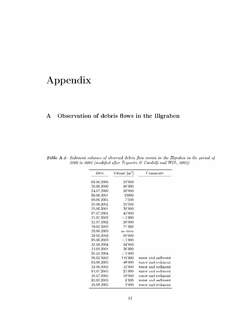
Appendix
A Observation of debris �ows in the Illgraben
Table A.1: Sediment volumes of observed debris �ow events in the Illgraben in the period of2000 to 2005 (modi�ed after Teysseire & Candol� and WSL, 2005).
Date Volume [m3] Comments
03.06.2000 10'00028.06.2000 90'00024.07.2000 20'00006.06.2001 3200009.06.2001 7'50015.06.2001 10'50028.06.2001 36'00007.07.2001 45'00021.07.2002 <5'00031.07.2002 20'00010.08.2002 71'00029.06.2003 no data19.05.2003 90'00008.06.2003 <5'00012.08.2004 34'00024.08.2004 36'00026.10.2004 <5'00028.05.2005 140'000 water and sediment03.06.2005 48'000 water and sediment13.06.2005 25'000 water and sediment04.07.2005 25'000 water and sediment18.07.2005 19'000 water and sediment02.08.2005 6'800 water and sediment18.08.2005 3'000 water and sediment
81
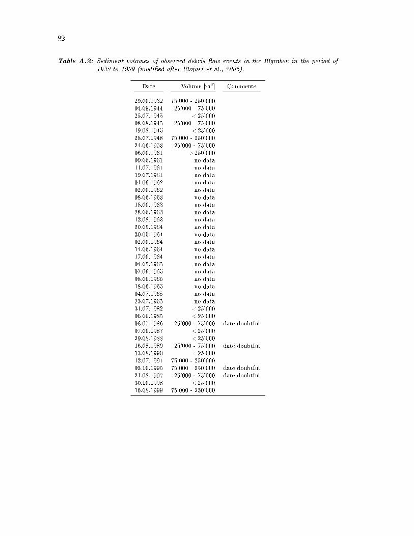
82
Table A.2: Sediment volumes of observed debris �ow events in the Illgraben in the period of1932 to 1999 (modi�ed after Rhyner et al., 2005).
Date Volume [m3] Comments
29.06.1932 75'000 - 250'00004.09.1944 25'000 - 75'00025.07.1945 <25'00008.08.1945 25'000 - 75'00019.08.1945 <25'00028.07.1948 75'000 - 250'00024.06.1953 25'000 - 75'00006.06.1961 >250'00009.06.1961 no data11.07.1961 no data19.07.1961 no data01.06.1962 no data02.06.1962 no data08.06.1963 no data18.06.1963 no data28.06.1963 no data12.08.1963 no data20.05.1964 no data30.05.1964 no data02.06.1964 no data14.06.1964 no data17.06.1964 no data04.05.1965 no data07.06.1965 no data08.06.1965 no data18.06.1965 no data04.07.1965 no data25.07.1965 no data31.07.1982 <25'00006.06.1985 <25'00006.07.1986 25'000 - 75'000 date doubtful07.06.1987 <25'00029.08.1988 <25'00016.08.1989 25'000 - 75'000 date doubtful13.08.1990 <25'00012.07.1991 75'000 - 250'00003.10.1995 75'000 - 250'000 date doubtful21.08.1997 25'000 - 75'000 date doubtful30.10.1998 <25'00016.08.1999 75'000 - 250'000

References 83
B ROC plots and accuracy statistic T
0.7
50.8
0.8
50.9
0.9
51
0.7
5
0.8
0.8
5
0.9
0.9
51R
eceiv
er-
opera
ting c
hara
cte
ristics (
RO
C)-
plo
t of
bed 1
specific
ity
(tru
e n
egative f
raction)
sensitivity (true positive fraction)
0.7
50.8
0.8
50.9
0.9
51
0.7
5
0.8
0.8
5
0.9
0.9
51R
eceiv
er-
opera
ting c
hara
cte
ristics (
RO
C)-
plo
t of
bed 2
specific
ity
(tru
e n
egative f
raction)
sensitivity (true positive fraction)
0.7
50.8
0.8
50.9
0.9
51
0.7
5
0.8
0.8
5
0.9
0.9
51R
eceiv
er-
opera
ting c
hara
cte
ristics (
RO
C)-
plo
t of
bed 3
specific
ity
(tru
e n
egative f
raction)
sensitivity (true positive fraction)
05
10
15
20
25
30
35
40
1.7
8
1.8
1.8
2
1.8
4
1.8
6
1.8
8
1.9
1.9
2
1.9
4
1.9
6
Accura
cy
sta
tistic T
as a
function o
f k
st
roughness c
oeff
icie
nt k
st
T = sum of sensitivity and specificity
bed 1
bed 2
bed 3
Figure B.1: Receiver-operation characteristics (ROC) plot and accuracy statistic T for thedi�erent subreaches.