Sediment suspension and turbulence in the swash zone of ... · Sediment suspension and turbulence in the swash zone of dissipative beaches Troels Aagaard a,⁎, Michael G. Hughes

(2006) 117–135www.elsevier.com/locate/margeo

Marine Geology 228

Sediment suspension and turbulence in the swash zoneof dissipative beaches

Troels Aagaard a,⁎, Michael G. Hughes b

a Institute of Geography, University of Copenhagen, Øster Voldgade 10, DK-1350 Copenhagen K., Denmarkb School of Geosciences, University of Sydney, Sydney NSW 2006, Australia

Received 21 February 2005; received in revised form 9 January 2006; accepted 12 January 2006

Abstract

This paper investigates mechanisms for stirring and transport of suspended sediment by infragravity-scale swash using high-frequency field measurements of horizontal and vertical flow velocities, water depths and sediment concentration profiles. The fielddata suggest that vertical velocity fluctuations generated by coherent eddies can be important to the process of sediment suspensionand can contribute to asymmetrically distributed sediment transport rates between the uprush and backwash phases of the swashcycle. This result indicates that the traditional and often used proxy for bed shear stress based solely on measurements of thehorizontal component of flow, u (i.e. τb∝ρfu2 where ρ is the water density and f is a friction factor) may be inadequate when usedin energetics-type sediment transport models applied to the swash, which is indeed the case. We demonstrate that a bed shear stressformulation which is more consistent with the physics leads to improved predictive capability for energetics-type transport models.This formulation is based on the correlation between the horizontal and (turbulent) vertical components of the flow (i.e. τb∝ρ(uw′).Despite the improvement, it is evident that considerable amounts of calibration data are still required before each application of thismodel type. Moreover, our data shows that the issue of calibration coefficients is more problematic than generally appreciated. Thecalibration coefficients for energetics-type models on a given beach not only differ between uprush and backwash, but also vary withposition within the swash zone, particularly on the uprush phase.© 2006 Elsevier B.V. All rights reserved.

Keywords: sediment transport; sediment suspension; swash zone; bed shear stress; turbulence; advection

1. Introduction

The swash zone is defined as that part of the beachprofile where the shoreline sweeps back and forth atfrequencies related to incident short waves (sea andswell) and infragravity waves. In the swash zone, theprofile is therefore subaerially exposed for part of eachswash cycle. The swa sh zone is an imp ortant and

⁎ Corresponding author.E-mail addresses: [email protected] (T. Aagaard),

[email protected] (M.G. Hughes).

0025-3227/$ - see front matter © 2006 Elsevier B.V. All rights reserved.doi:10.1016/j.margeo.2006.01.003

integral part of the beach/shoreface environment,because swash processes largely determine whetherthe subaerial beach erodes or accretes and large amountsof sediment are suspended and transported in continu-ous exchange between the nearshore and the foreshore.

Basically two types of swash regime exist: On steepbeaches swash is predominantly driven by short waves(sea and swell) whereas on gently sloping dissipativebeaches it is predominantly driven by infragravitywaves. Foreshore accretion and an increase in beachface slope against the force of gravity require anasymmetry in the sediment transport field caused by

mailto:[email protected]

mailto:[email protected]

http://dx.doi.org/10.1016/j.margeo.2006.01.003

118 T. Aagaard, M.G. Hughes / Marine Geology 228 (2006) 117–135

either asymmetric uprush/backwash velocities or anasymmetry in the amounts of sand suspended on theuprush and the backwash. Accordingly, field observa-tions show that suspended sediment concentrations areoften larger on the uprush than in the backwash (Puleo etal., 2000; Butt et al., 2002; Masselink et al., 2005;Hughes et al., in press).

A considerable effort has been invested in attemptingto model sediment transport in the swash zone. Bagnold-type energetics models for bedload (Bagnold, 1963),which predict a dependence of sediment transport onvelocity skewness, have been particularly popular (e.g.Hughes et al., 1997a; Masselink and Hughes, 1998;Puleo et al., 2000). These models relate sedimenttransport, q, to velocity cubed through q=ku3, where kis a calibration coefficient incorporating friction that isexpected to be constant for a given beach. In general,mixed results have been obtained, because field testssuggest that the uprush is more ‘efficient’ than thebackwash, i.e. kupNkback (e.g. Masselink and Hughes,1998; Puleo et al., 2000). Such results are consistent withthe laboratory findings of Cox et al. (2000) and Conleyand Griffin (2004) who observed larger mean bed shearstresses and friction factors in the uprush compared withthe backwash, suggesting that Bagnold-type modelsomit some important physics. Several explanations havebeen offered for larger bed shear stresses and sedimenttransport in the uprush. These include: (a) accelerationeffects induced by landward directed pressure gradients(Butt and Russell, 1999; Nielsen, 2002; Puleo et al.,2003); (b) turbulence impinging on the bed caused bybores overrunning the preceding swash lens or advectedfrom bore collapse (Puleo et al., 2000; Petti and Longo,2001; Butt et al., 2004); (c) sediment advection from thepoint of bore collapse (Hughes et al., 1997b, in press;Pritchard and Hogg, 2005); and/or (d) groundwater in/exfiltration modifying the fluid boundary layer (Turnerand Masselink, 1998; Butt et al., 2001). Added to theomission of these potentially important processes inexisting bedload models is the uncertainty of theirrelevance in situations when large amounts of sand aretransported in suspension.

As listed above, turbulence is one of the potentiallyimportant contributors to sediment suspension in thenearshore/swash zones. Surf zone breakers generatelarge vortices that can penetrate to the bed and generatelarge vertical velocity oscillations (Nadaoka et al., 1988;Smyth et al., 2002) and Reynolds-stresses (Yu et al.,1993; Cox and Kobayashi, 2000). This bore-relatedturbulence can be injected into the swash zone at borecollapse and can be advected along by the swash frontwith the turbulent face in contact with the bed.

Additional sources of turbulence generated within theswash zone include hydraulic jumps at the end of longinfragravity backwash events; incoming bores overrun-ning the preceding swash lens, and friction at the bed. Inmost previous field studies of swash zone sedimenttransport, only horizontal flow components have beenobtained, exceptions being the data sets of Osborne andRooker (1999) and Butt et al. (2004). As a result, theeffects of bore-generated turbulence and eddies, includ-ing vertical velocity fluctuations, have not been directlyquantified in the context of sediment resuspension andtransport in the field.

In this paper, observations are reported on near-bedhorizontal and vertical velocity structure and theensuing sediment resuspension and transport on two(dissipative) beaches dominated by uprush/backwash atinfragravity time scales. The aims of the paper are: (i) toexamine the spatial structure of sediment transport indissipative swash and to identify zones of erosion andaccretion, (ii) to examine the nature of turbulence in theswash and to quantify its importance to sedimentresuspension and transport and (iii) to test a newmodel for sediment concentration in which bed shearstresses, calculated as the covariance of the horizontaland vertical velocity components, are used to parame-terize sediment stirring. While still not satisfactory, thismodel shows significantly improved skill comparedwith the widely used Bagnold-type model.

2. Theoretical background

Several existing sediment transport models for thesurf zone (e.g. Bagnold, 1963; Bailard, 1981) predictsediment concentration/load (c) as a function of asediment stirring term which is parameterized throughthe horizontal velocity variance

c ¼ k1U2 ð1Þ

where U is the vector product of cross-shore andlongshore velocity (U=(u2 +v2)½) and k1 is a constantof proportionality incorporating friction. If the long-shore velocity component is zero, sediment transport (q)is then the product of the stirring term and a transportterm which is the fluid velocity, i.e.

q ¼ k1u3: ð2Þ

This formulation is based on the concept that bedshear stress (τb) which is responsible for sedimentstirring, can be expressed through

sb ¼ qcfu2 ð3Þ

where ρ is fluid density and cf is a coefficient of friction.

119T. Aagaard, M.G. Hughes / Marine Geology 228 (2006) 117–135

In the present work we are primarily concerned withsuspended load. Furthermore, instead of using a bedshear stress proxy such as Eq. (3) we consider an explicitformulation for bed shear stress. Using the Reynoldsequation for combined wave–current flow in a turbulentoscillatory boundary layer and neglecting the steadycurrent contribution, the turbulent momentum flux inthe cross-shore dimension is defined as

mtdudz

¼ sq¼ − u wð Þ− u Vw Vð Þ þ m ð4Þ

(e.g. Nielsen, 1992, p.31), where νt is eddy viscosity, τis horizontal (bed) shear stress, u,w are the cross-shoreand vertical velocity components, ν is kinematic(laminar) viscosity and tildes and primes denote orbitaland turbulent velocity contributions, respectively. As-suming laminar viscosity is negligible, the bed shearstress is made up of two terms: one due to wave motionsand one due to turbulence (Reynolds stresses) and basedon Eq. (4), a model for sediment concentrations in theswash zone can be expressed as

c ¼ k2juwj ð5ÞIn principle, |uw| includes orbital as well as turbulent

velocity components. Multiplying Eq. (5) by the cross-shore velocity results in a crude model for sedimenttransport in the swash zone which is analogous to theBagnold-type formulation (Eq. (2)) consisting of astirring term and a transport term,

q ¼ k2juwju ð6Þ

To specifically examine turbulence characteristicsand the significance of turbulence to sediment resuspen-sion, the turbulent signal must be extracted from themeasured time series of u and w to isolate the turbulentkinetic energy,

TKE ¼ 1=2qðu V2 þ m V2 þ w V2Þ ð7Þ

However, the separation of orbital and turbulentvelocity terms using measurements from a singleinstrument in irregular and strongly nonlinear waveconditions with potentially slight misalignments insensor orientation is not a trivial task (Trowbridge,1998). Various methods have been proposed oftenemploying a high-pass filter with a specified frequencycut-off to remove orbital motions. This cut-off has beenbased on either coherence between the velocity andsurface elevation signals (Thornton, 1979), excessmeasured velocity variance relative to predicted orbitalvelocity variance (Rodriguez et al., 1999), or spectral

slope breaks (Smyth and Hay, 2003; Scott et al., 2005).At the outset, we take the pragmatic view that close tothe bed, contributions to the vertical velocity fromwave-orbital motions (w) are expected to become small,especially in the very shallow water depths of the swashzone where vertical wave orbital velocities tend to zero.This is consistent with the data presented in Section 4.3.As the assumption is equivalent to making theassumption that the flow is hydrostatic, it is alsoconsistent with several numerical models which makethat latter assumption and successfully describe theessential features of the flow in the inner surf and swashzones with a good degree of accuracy (e.g. Hibberd andPeregrine, 1979; Kobayashi et al., 1989; Watson andPeregrine, 1992 and several others). Furthermore, if weassume that w′ is some fixed proportion of u′ (and v′) onthe time scale of turbulent vortices (Svendsen, 1987),the turbulent kinetic energy (and the sediment concen-tration in the water column due to Reynolds stresses)should scale as the vertical velocity variance,

TKE~w V2~w2 ð8Þ

3. Field sites and instrumentation

3.1. Field experiments

Two field experiments were conducted at Skallingenon the Danish North Sea coast during August–September 2002 and at Egmond aan Zee on the CentralDutch coast during October–November 2002. Skallin-gen is a dissipative beach with a gently sloping, low-relief double-barred inner nearshore (surf) zone. Themean annual significant wave height is 1.0m and themean tidal range is 1.5m, which increases to 1.8mduring spring tides and the intertidal zone typicallyexhibits one or more intertidal bars. At the time of theexperiment, the foreshore sediment was moderatelysorted with a mean grain size of 240 μm and the beachface slope was β=0.032 (Fig. 1). Wave energy levelsduring the experiment were quite low; significantoffshore wave heights mostly remained below 0.5–0.6m, but increased briefly up to 2.1m, and theincident wave periods ranged from 4 to 8s (Aagaard etal., 2005). Measurements from a pressure sensorinstalled at x=120m (Fig. 1) showed that thesignificant wave height at the base of the swash zonedid not exceed 0.6m and the Iribarren number at theforeshore was between 0.3 and 0.4, which indicatesspilling breakers and dissipative conditions in the innersurf/swash zone.

Fig. 1. Beach profiles from Egmond (solid line) and Skallingen(dashed). The locations of the swash zone instrument stations areindicated (E=Egmond, S=Skallingen). MWL is mean water level.


At Egmond the longshore bars are larger and higherthan at Skallingen, with deep intervening troughs andthe surf zone morphology is modally intermediate. Theaverage annual significant wave height is approximately1.2m and the mean semi-diurnal tidal range is 1.65m,which increases to 2.1m at springs. The tidal curve isasymmetric with a 4-h flood period and an 8-h ebb-period. The mean sediment grain size in the intertidalzone was slightly coarser than at Skallingen, 260 μm,and the sand was very well-sorted. The beach face slopewas β=0.036. Wave energy conditions during the periodof data collection were much more energetic than atSkallingen. Significant offshore wave heights were up to3.75m with wave periods of 6–9s and maximuminshore wave heights at x=126m (Fig. 1) were 1.25m(Aagaard et al., in press) with a foreshore Iribarren-

Fig. 2. Photo of the swash zone instrument station. ADV is the acoustic curreOBS is the vertical array of optical backscatter sensors, EM is the electroma

number of approximately 0.3, again indicating dissipa-tive conditions in the inner surf/swash zone.

3.2. Instrumentation

Cross-shore instrument arrays were deployed acrossthe intertidal and inner nearshore zones at both sites.However, only results from the intertidal stations(shown in Fig. 1) are reported here. Instruments weremounted on a stainless steel H-frame (Fig. 2) andconsisted of a 3D sideways-looking Sontek 10MHzAcoustic Doppler Velocimeter (ADV) mounted with thehorizontal axes parallel to the bed at a nominal elevationof 0.025–0.03m and a vertical array of five D&AInstruments UFOBS-7 fibreoptical backscatter sensors.The UFOBS-7 uses an infrared laser beam with a passband of 810–850nm to detect sediment concentrationwithin a very small sampling volume (nominally≈10mm3) that is centred 10–15mm away from thesensor head. Due to the small size of the sensor head(8mm O.D.) and the remote sampling volume, theinstrument is capable of recording sediment concentra-tions very close to the bed. In this experiment samplingvolumes were nominally centred at z=0.01, 0.02, 0.03,0.04 and 0.05m. Similar to the ordinary D&A Instru-ments OBS-sensors, the UFOBS is not sensitive tovisible light. Infrared radiation from the sun can saturateOBS-sensors when exposed to direct sunlight, orsunlight reflected from the water surface or foam. Thisis easily identified in the records, which become

nt meter, UFOBS is the vertical array of fibreoptic backscatter sensors,gnetic current meter and PT is the pressure transducer.


extremely spiky and concentration profiles becomeinverted as the uppermost sensor is most stronglyaffected. In the present experiment, such problems wereavoided by pointing the sensors downwards and/oraway from the sun. No cases of measurement errors dueto ambient infrared/daylight exposure could be identi-fied for the UFOBS-7 sensors.

ADVs can accurately measure mean currents andorbital velocities at elevations equal to, or larger, thanthe vertical extent of the sampling volume (Voulgarisand Trowbridge, 1998) which is 9mm for the instrumentin question. With the deployment elevations used here,the ADV was capable of recording horizontal andvertical flows in water depths of ≈0.03–0.04 and0.07m, respectively.

Ancillary instruments consisted of a pressure sensor(Druck Model PTX1830) which was deployed at, orslightly below, bed level in order to measure waterdepths, a Marsh-McBirney OEM512 electromagneticcurrent meter (EM) at a nominal elevation of 0.20mabove the bed, and an array of three D&A InstrumentsOBS-1P optical backscatter sensors at nominal eleva-tions of 0.05, 0.10 and 0.20m above the bed. Instrumentelevations were measured prior to and after eachinstrument run and elevations were adjusted if requiredand when possible. Sensors were hard-wired to shorewhere the signals were recorded on laptop computers.

3.3. Data collection, processing and analysis

(UF)OBS-sensors were post-calibrated in a largerecirculation tank using sand samples from the deploy-ment locations. Known quantities of sand werecumulatively added to the tank, water samples weredrawn off and sensor output recorded to construct acalibration curve for the particular sand grain reflectancecharacteristics at the two sites. Field offsets weredetermined from distinct breaks in the cumulativefrequency distribution of sediment concentration.These offsets were close to the 2nd and 5th percentilefrequency output voltages for the UFOBS- and OBS-sensors, respectively, and to maintain consistency thesepercentiles were applied to all records.

During periods of data collection, instruments weresampled almost continuously at 10Hz. The duration ofindividual records was 45min and records wereseparated by 2–5min breaks to back up data. Instrumentoutputs were screened and checked for data quality andrecords containing instrument noise and/or erroneousdata were rejected. The saturation level of the UFOBS-sensors was 100–120kg m−3 for the grain sizes atEgmond and Skallingen while OBS-sensors saturated at

105–140kg m−3. Records containing N2% of clippedvalues due to sensor saturation were discarded as thesensor in question was probably within, or at, the bed. Itis possible that extreme suspension events also resultedin saturation, thus these events are excluded from ourdata.

Velocity time series from an ADV tend to becomenoisy in highly turbulent or aerated flows. At such times,signal correlation values recorded by the ADV wereused to quality control the data. For the samplingfrequency used here the threshold signal correlationindicating potentially inaccurate data for a particularacoustic beam was b55% (Raubenheimer, 2002). Alow-pass filtered record of the original velocity timeseries was obtained using a filter cut-off frequency of2.5Hz. Observations in the original velocity time seriesthat had a signal correlation below the threshold werereplaced with the corresponding observation from thefiltered time series. Furthermore, a conservativelyselected signal-to-noise ratio of b20 (SonTek, 2001)was employed to identify occasions when the sensorbecame emerged; at such times, the flow velocity isundefined (Hughes and Baldock, 2004).

Pressure sensors were calibrated in a stilling well atthe field site and pressure records were detrended priorto computing wave heights. Mean water depths andwater levels were determined through repeated surveysof instrument positions and measurements of sensorelevations relative to the bed. Instantaneous sedimentflux at a point was calculated as the product of localsediment concentration (c) and fluid velocity (u). Netcross-shore suspended sediment fluxes at the respectivesensor elevations were then calculated as

qz ¼ huci ð9Þwhere ⟨⟩ denotes the time-average. The fluxes deter-mined from the UFOBS-sensors each represented a0.01m vertical bin while the two upper OBS-sensorseach represented 0.10m bins. Fluxes were subsequentlysummed across the instrument array and linearlyextrapolated to the water surface to yield approximaterun-averaged net suspended sediment transport rates.The sediment transport was computed using velocitiesfrom the ADV with sediment concentrations determinedfrom the UFOBS-array, and velocities from the EMwithconcentrations from the OBS-array. Coupling velocitymeasurements at one elevation with measurements ofsuspended sediment concentration at another canpotentially result in erroneous estimates, particularlywithin the bottom boundary layer (e.g. Ogston andSternberg, 1995). We sought to minimise this potentialproblem by matching the ADV-elevation to the middle


sensor in the UFOBS-array. In addition, the shallow,rapid flows in the swash zone can be expected to be verywell mixed.

4. Results

4.1. Observed sediment transport rates in the swashzone

A total of 25 swash zone records (each of 45 minduration) containing reliable velocity and sedimentconcentration data were obtained. Net sediment trans-port rates depended strongly upon relative positionwithin the swash zone. To distinguish such differentrelative positions, the upper, mid and lower swash zoneswere separated on the basis of the fraction of time thatthe ADV was immersed during a run (i.e. a signal-to-noise ratio N20 on the cross-shore acoustic beam).Upper swash zone conditions were assigned when theADV was immersed for 1–40% of an instrument run,mid swash conditions for 40–75% and lower swashconditions for 75–95% immersion.

The net suspended sediment transport exhibitedsimilar overall characteristics at the two beaches (Fig.3). Transport was relatively small and onshore directedwhen sensors were located in the uppermost swash zoneat low tidal stages. With an increased fraction ofinstrument immersion, i.e. for increasing mean water

Fig. 3. Net suspended sediment transport rates (qs) at Egmond (E) andSkallingen (S), as a function of the fraction of time that the ADV-sensor was immersed. The data have been separated into rising andfalling tidal stages. The solid line is a second-order polynomial fitthrough all data points.

levels, onshore transport rates also increased whereasthe transport reversed and became large and offshoredirected when instruments were located in the lowerswash zone. Net transports in the inner surf zone werealso seaward directed (Aagaard et al., 2005, in press).There was no obvious difference in net transport ratesrecorded on rising and falling tides (Fig. 3).

A second-order polynomial was fitted through alldata points to define a sediment transport shape functionfor the swash zones of these two dissipative beaches.The empirical function is

y ¼ −0:00043x2 þ 0:032x−0:08

where y is net sediment transport rate and x is percentageof immersion. Maximum onshore transport ratesoccurred around the transition between the mid andupper swash zones (as defined here), and maximumoffshore transport rates occurred at the base of the swash(Fig. 3).

4.2. Fluid velocity and sediment concentration in theswash zone

In order to examine the relationships between fluidvelocity and sediment concentration, six example timeseries were selected to represent respectively upperswash (runs EG07; 24% instrument immersion andEG44; 38% immersion), mid swash (runs EG59; 53%immersion and EG45; 66% immersion) and lower swash(runs EG46; 90% immersion and EG68; 94% immer-sion) conditions. The time series were selected on thebasis of four criteria: (a) swash flows had to besufficiently deep to yield reliable estimates of w, i.e.time series of vertical velocities should be continuousthrough individual swash events, although this criterionhad to be relaxed for upper swash records; (b) the ADVshould be within 4cm from the level of the bed; (c) thelowermost fibreoptical sensor should be within 2cmfrom the bed, and (d) signal saturation in fibreopticalsensors should be b2 % of the record length for at least 4of the sensors. Fig. 4 illustrates an example of recordedcumulative frequency distributions of sediment concen-tration at different levels above the bed. For thisparticular record, the lowermost UFOBS-sensor satu-rated for 1.1% of the record, indicated by the break-offat the top of the curve, the uppermost sensor (which hada significantly higher gain than the rest of the sensors)saturated for 2.3% of the time whereas the middle sensordid not saturate.

All examples selected on the basis of these criteriawere from the Egmond-experiment because swash flows

Fig. 4. Cumulative frequency distributions of sediment concentrationsmeasured by the UFOBS sensors at z=0.01, 0.03 and 0.05m in the midswash zone; run EG59.


were deeper and vertical velocity estimates were morecontinuous and reliable during swash events. Represen-tative 2min time series of cross-shore (u) and vertical(w) velocities, and sediment concentrations at z=0.01mand 0.03m are illustrated in Figs. 5, 6 and 7. In allexamples, the velocity sensor was located ≈0.025–0.035m above the bed and positive velocities aredirected onshore and upwards in the figures.

Uprush velocities were large in the upper swashzone, up to ≈1.5 m s−1 (Fig. 5). Velocity distributionswere characteristically asymmetric, which may, at least

Fig. 5. Two-minute time series of (upper panel) cross-shore velocity and (lowez=0.03m (dashed line) in the upper swash zone; run EG07. Positive velocit

in part, be due to the fact that the sensor becameemerged in the final stages of the backwash. Sedimentconcentration events were also asymmetrically distrib-uted, however, with conspicuously larger concentrationsduring the uprush (up to 100kg m−3) compared with thebackwash (20–40kg m−3). Vertical velocities observedduring the backwash in this record from the upper swashzone did not meet the data quality criteria and have beenomitted.

In the mid swash (Fig. 6), the cross-shore velocityfield was more symmetric with respect to peak velocitiesalthough the uprush flow was of shorter duration. Ingeneral, sediment concentrations were still asymmetri-cally distributed with larger concentrations during theuprush, which resulted in a net onshore directedsuspended sediment transport. The time series ofvertical velocities reveals significant amounts of high-frequency turbulence throughout swash events. Moreprolonged, predominantly downward directed verticalvelocity fluctuations with speeds up to ≈1m s−1 occurat the leading edge of the swash and at the end ofprolonged backwash cycles. Downward directed veloc-ities on the uprush are inconsistent with wave motionsand the time scale of the vertical fluctuations (1.5–3.5s)is distinctly shorter than the cross-shore orbital wavevelocity time scale. Hence, it is unlikely that thesevertical fluctuations were directly associated with localwave orbital motions.

The lower swash zone (Fig. 7) was characterized byextended backwash events during which the cross-shorevelocity sometimes exceeded 1.5m s−1. Such events

r panel) suspended sediment concentration at z=0.01m (solid line) andies are directed onshore.

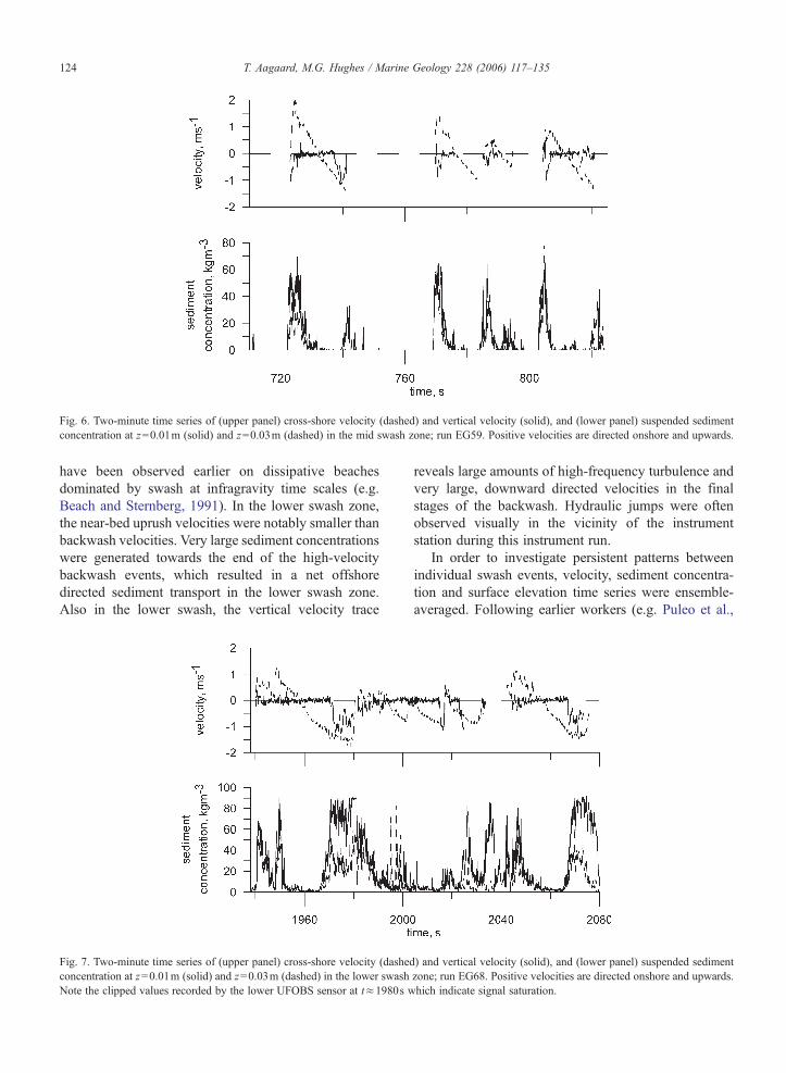
Fig. 6. Two-minute time series of (upper panel) cross-shore velocity (dashed) and vertical velocity (solid), and (lower panel) suspended sedimentconcentration at z=0.01m (solid) and z=0.03m (dashed) in the mid swash zone; run EG59. Positive velocities are directed onshore and upwards.


have been observed earlier on dissipative beachesdominated by swash at infragravity time scales (e.g.Beach and Sternberg, 1991). In the lower swash zone,the near-bed uprush velocities were notably smaller thanbackwash velocities. Very large sediment concentrationswere generated towards the end of the high-velocitybackwash events, which resulted in a net offshoredirected sediment transport in the lower swash zone.Also in the lower swash, the vertical velocity trace

Fig. 7. Two-minute time series of (upper panel) cross-shore velocity (dashedconcentration at z=0.01m (solid) and z=0.03m (dashed) in the lower swashNote the clipped values recorded by the lower UFOBS sensor at t≈1980s w

reveals large amounts of high-frequency turbulence andvery large, downward directed velocities in the finalstages of the backwash. Hydraulic jumps were oftenobserved visually in the vicinity of the instrumentstation during this instrument run.

In order to investigate persistent patterns betweenindividual swash events, velocity, sediment concentra-tion and surface elevation time series were ensemble-averaged. Following earlier workers (e.g. Puleo et al.,

) and vertical velocity (solid), and (lower panel) suspended sedimentzone; run EG68. Positive velocities are directed onshore and upwards.hich indicate signal saturation.


2000; Masselink et al., 2005), single swash events wereextracted from the time series and re-sampled on anormalized time scale, t/T, where T is the duration of theindividual swash event. Twenty averaging bins atintervals of t/T=0.05 were used. Table 1 lists thenumber of individual swash events extracted and themean swash duration for the six example time series aswell as offshore and inshore wave conditions. Ensem-ble-averaged time series of cross-shore velocity (u),vertical velocity variance (w2, which is proportional tothe turbulent kinetic energy (Eq. (8)) and the (turbulent)bed shear stress), surface elevation (z), Froude number(Fr) and sediment concentration (c) were obtained. w2

has been recast in terms of |w|w in order to illustrate thedominant direction of the vertical velocity component.

The ensemble-averaged time series from the upperswash zone are illustrated in Fig. 8. Wave conditionswere moderate with offshore significant wave heightsand peak spectral wave periods of 1.8m and 5.6s,respectively (Table 1). The plots illustrate that meansediment concentrations were very large during theuprush and small during the backwash, in correspon-dence with the relatively large uprush velocitiescompared to the backwash. The flow was subcriticalthroughout the swash cycle. The vertical velocityvariance has not been included during the backwashphase due to the shallow water depths which preventedreliable w-estimates. During the uprush there was norelationship between sediment concentration and therecorded vertical velocity variance, which had no clearstructure.

The example representing the mid swash zone (Fig.9) was obtained under high-energy conditions withoffshore wave heights and periods of Hs,0=3.5m andTp,0=7.1s (Table 1). Sediment concentrations wereasymmetrically distributed with larger concentrationsduring the uprush, even though the cross-shore velocityfield was skewed offshore. Visually, it appears that there

Table 1Summary statistics of selected swash time series and offshore andinshore wave conditions

Run No. ofswash events

Meanduration (s)

Hs,0

(m)Tp,0(s)

Hs,i

(m)Tp,i(s)

EG07 (upper) 43 12.5 1.8 5.6 0.29 38EG44 (upper) 18 22.6 2.9 7.7 0.41 50EG45 (mid) 31 27.5 3.5 7.1 0.42 50EG59 (mid) 29 22.8 3.3 7.1 0.44 58EG46 (lower) 20 41.0 3.3 7.1 0.50 55EG68 (lower) 40 44.9 2.4 7.1 0.39 58

Offshore wave parameters are indicated by subscript 0 and waveparameters measured at the base of the swash zone are indicated bysubscript i.

is a good correspondence between the concentrationrecords and both the u and |w|w-traces. However, theincrease in c at t/T=0.875 is more in accordance withthe turbulent signal (|w|w), which increases rapidly at thesame relative phase and in association with a transitionto supercritical flow. In the mid swash, the |w|w-trace isconsistently exhibiting large downward directed veloc-ities at the leading edge of the uprush and at thetermination of backwash, as also observed in theinstantaneous velocity time series (Fig. 6). There is aclear hysteresis effect evident; during the uprush c isslow to decrease during the waning of the large verticalvelocities and during the backwash c is slow to increaseduring the waxing of the large vertical velocities. Thesurface elevation trace from this record (z) is irregulardue to the superposition of several short wave bores onthe infragravity-scale swash events.

The example selected for lower swash zone condi-tions (Fig. 10) was obtained under decaying storm waveconditions with Hs,0=2.4m and Tp,0=7.1s (Table 1).The cross-shore velocity and surface elevation traces areagain quite irregular due to several short wave cyclesoccurring during an individual infragravity swash event.Sediment concentrations are comparatively largethroughout the swash cycle with maxima at the leadingedge of the uprush and, in particular, at the terminationof the backwash. Throughout the cycle, changes inconcentration agree qualitatively well with fluctuationsin |w|w although concentrations seem to be dispropor-tionately large at the leading swash edge and hysteresisis again evident. The Froude number exceeds 1 in thelate stages of the backwash, but sediment concentrationsclearly increase prior to the onset of supercritical flowconditions and they follow more closely the |w|w-trace.

4.3. Vertical velocity structure

Visual comparisons between velocity and sedimentconcentration traces in Figs. 8, 9 and 10 suggest thatvertical velocity variance may be important to sedimentsuspension in the mid and lower swash zones. Thequestion is whether these velocity fluctuations areindeed due to turbulence, i.e. whether w2 is a suitablesurrogate for the turbulent kinetic energy (Eq. (8)). Atthe leading edge of the uprush, large, downwarddirected velocities occurred. Their magnitude (0.5–1ms−1) and time scale (several seconds, but shorter than thecross-shore velocity time scale; Figs. 6 and 7) suggestthat they are not due to ordinary wall turbulencegenerated by bed friction. On the other hand, thevertical velocity is mainly negative in sign (i.e. directedtowards the bed), which suggests that the velocity

Fig. 8. Ensemble-averaged records of cross-shore velocity (u), surface elevation (z), vertical velocity variance (w|w|), Froude number (Fr) andsediment concentration (c) at z=0.01m (solid) and z=0.03m (dashed line); upper swash zone conditions, run EG07.


fluctuations are also not due to wave orbital motion. Atthe termination of the backwash, even more prolonged(5–8s), high velocity (−0.5 to 1m s−1) fluctuationswere observed at times when the flow becamesupercritical (e.g. Figs. 7 and 10).

The individual swash events were concatenated toform continuous time series of cross-shore and verticalvelocity. Spectra from these time series (Fig. 11) showthat vertical velocity variance decreased approximatelyas f −5/3 between 0.1 and ≈2Hz, consistent with aninertial subrange which further indicates this frequencyband is in fact dominated by turbulent motions (Kundu,1990; Smyth and Hay, 2003). Beyond 2Hz, verticalvelocity variance appears to approach a backgroundnoise floor; this break-off frequency is somewhat lower

than the 4.5Hz observed by Raubenheimer et al. (2004).In contrast, the slope of the cross-shore velocityspectrum at frequencies 0.1–2Hz is intermediatebetween f −3 and f −5/3, which is consistent with amixture of turbulence and saturated wave motion whichis expected to decay as f −3 (e.g. Thornton, 1979).

As the frequency band characterized by an f −5/3

spectral roll-off (i.e. 0.1–2Hz) was probably dominatedby turbulent motions, turbulence constituted 74–95% ofthe total vertical velocity variance (after subtracting thenoise floor) in the four example time series from the midand lower swash zones. Thus, a major fraction of thevertical velocity fluctuations had a short-wave timescale, but were not directly due to wave orbital motions.It seems reasonable, therefore, to include the prolonged

Fig. 9. Ensemble-averaged records of cross-shore velocity (u), surface elevation (z), vertical velocity variance (w|w|), Froude number (Fr) andsediment concentration (c) at z=0.01m (solid), z=0.03m (small dashes) and z=0.05m (large dashes); mid swash zone conditions, run EG45.


(several seconds duration) high-speed events in esti-mates of swash zone turbulence.

4.4. Sediment resuspension mechanisms

To more quantitatively examine the relationshipsbetween sediment concentration and resuspensionmechanisms, Eqs. (1) and (5) were tested throughcalculation of the total sediment load (C) in thewater column by summing the loads in each measure-ment bin:

C ¼Xh

z¼0:05

cðzÞDz ð10Þ

where h is water depth andΔz is 0.01m for the UFOBS-sensors and 0.10m for the OBS-sensors with theconstraint that c=0 at the water surface. Instantaneousloads were correlated with instantaneous values of U2,U3 and |Uw| where U is computed as the vector productof cross-shore and longshore velocity and |Uw| includesorbital motions, contained in U and turbulent motionswhich make up the majority of w. This approach followsearlier attempts at estimating relationships betweenenergetics-type models and sediment transport, but inthis case we consider the sediment concentration andavoid the spurious correlations introduced by includingcross-shore velocity in measurements of q (Puleo et al.,2005). Because w consists mainly of turbulent motions,

Fig. 10. Ensemble-averaged records of cross-shore velocity (u), surface elevation (z), vertical velocity variance (w|w|), Froude number (Fr) andsediment concentration (c) at z=0.01m (solid), z=0.03m (small dashes) and z=0.05m (large dashes); lower swash zone conditions, run EG68.


|Uw′| might be a more appropriate expression here than|Uw| but the latter is maintained because in principlew contains contributions from all frequency bands.

An example of these relationships is illustrated inFig. 12. While the correlations are statistically signifi-cant, they are certainly not convincing with r2 rangingfrom 0.081 (U2), 0.075 (U3) to 0.098 (|Uw|). Thereasons for the poor correlations are probably due to thedifferent time scales of velocity structure and sedimentresuspension events, partly demonstrated by the hyster-esis observed in the ensemble-averaged time series(Figs. 9 and 10), but much more evident and morevariable in the individual time series. Sedimentconcentrations remain high even after velocity hasdecreased (Figs. 6 and 7), probably due to settling lag

(Baldock et al., 2004) and the persistence of high-frequency, low-magnitude turbulence maintaining sandin suspension (see also Nielsen, 1993; Leeder et al.,2005). Additionally, on the stirring phase, it takes afinite time for the sediment to diffuse upward to theelevation of the optical sensors.

To reduce the problem of different time scales, thecorrelations were also performed with ensemble-aver-aged values of the different variables, i.e. averages ofU3, |Uw| and Cwere computed for the 20 phase bins (seealso Masselink et al., 2005). The reason for selecting U3

instead of U2 is that Bagnold-type models (as applied tothe surf zone) predict a dependency of suspendedsediment transport on the fourth moment of horizontalvelocity (e.g. Bailard, 1981) and hence sediment

Fig. 11. Example spectra of cross-shore (upper panel) and vertical(lower panel) velocity variance recorded in the mid (solid lines) andlower (dashed lines) swash zones.


concentration should depend on the third moment. Tests(not shown) also demonstrated that in general, correla-tions between U3 and C were marginally superior torelationships involving the squared velocity moment.

Ensemble-averaged suspended sediment loads wereleast-squares fitted to ensemble-averaged |Uw| and U3

for the 20 phase bins in the six example runs. The datawas separated into the uprush and backwash phases andr2-values for the least-squares regression models arelisted in Table 2. Using ensemble-averaged values vastlyimproves the functional relationships. With respect tothe mid and lower swash zones, |Uw| is a significantlybetter predictor than U3 except for backwash in thelower swash zone where the latter performs slightlybetter. In the upper swash zone, the (uprush) predictionsusing |Uw| are poor as vertical velocities were not well

resolved in these shallow water depths whereas thecubed horizontal velocity moment provided a reason-able fit.

The results of the regressions on |Uw| and U3 areillustrated graphically in Figs. 13 and 14. The figuresamply demonstrate that |Uw| is a significantly betterpredictor than U3, particularly in the uprush. However,calibration coefficients are different not only in theuprush and the backwash (as previously reported by e.g.Masselink and Hughes, 1998; Puleo et al., 2000) butalso at different relative positions within the swash zone,particularly during the uprush (Table 3). For the mid andlower swash zone data, k2 (Eq. (5)) ranges from 8.2 to23.6 for the uprush. For the backwash, the spread in k2 issmaller; 1.1–2.2.

All data from the mid and lower swash zones werecombined in Fig. 15 to assess the merits of a transportmodel based on estimated bed shear stress, includingturbulent Reynolds-stresses, as the stirring term. Thedata suggest that a sediment concentration model basedon |Uw| (mean skill=0.85 and 0.61 on the uprush andbackwash, respectively; Table 2) is clearly superior to amodel using U3 as the stirring mechanism. However, weare still faced with the problem of different calibrationcoefficients on the uprush (k2=9.5) and the backwash(k2=1.3) and it is indeed questionable whether therelationships obtained are generally applicable. It wouldappear that non-local factors contribute significantly tosediment concentrations observed within the swashzone.

5. Discussion

Measurements of suspended sediment transport atelevations of 1–20cm from the bed at two dissipativebeaches, dominated by swash at infragravity time scales,have indicated that this transport is almost alwayslandward directed in the mid and upper swash zones,and offshore directed in the lower swash zone (Fig. 3).This is consistent with sediment transport measurementsreported by Butt et al. (2002) and by Cox et al. (2000)who observed onshore directed mean bed shear stressesin the upper swash and offshore directed stresses in thelower swash. The swash zone of dissipative beachesthus seems to be segregated with respect to sedimenttransport and consequently such beaches should displaya tendency for accretion at the landward edge of theswash if accommodation space is available. With arising tide, the morphological change resulting from asediment transport ‘shape function’ such as the onedepicted in Fig. 3 is likely to be a progressive onshoretranslation of a wedge of sediment located at the upper

Fig. 12. Instantaneous sediment loads in the water column plotted against instantaneous (a) squared horizontal velocity, (b) cubed horizontal velocity,and (c) cross-product of horizontal and vertical velocity. The lines of best fit have r2=0.081 (a), 0.075 (b) and 0.098 (c). n=6601. Run EG59.


edge of the swash. With a falling tide, an offshoreprogressive erosion/accretion couplet should occur.Such morphological changes would agree with theobservations of Strahler (1966).

The reason for the onshore-directed sedimenttransport asymmetry was the increased sediment con-centrations during the uprush relative to the backwashand, for the upper swash zone, an onshore asymmetriccross-shore velocity field (Figs. 5 and 8). Because of thelarger sediment concentrations and larger water depths,sediment loads during the uprush were therefore largerthan during the backwash. In the mid swash, theconcentration asymmetry led to an onshore net sediment

transport in spite of the larger offshore directedvelocities (Figs. 6 and 9). In the lower swash zone,however, the net suspended sediment transport wasseaward directed at both beaches, due to large sedimentconcentrations and turbulence generation during thebackwash, associated with the transition to supercriticalflow conditions as well as an offshore directed velocityasymmetry (Figs. 7 and 10).

Examination of the time series of velocity andsediment concentration revealed that large concentra-tions were associated with prolonged large-magnitudevertical velocity fluctuations (Figs. 6–10) which,despite their incident wave time scale, were primarily

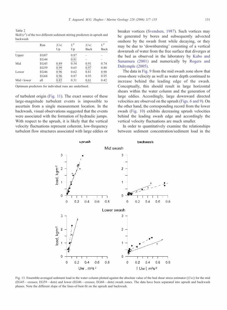
Table 2Skill (r2) of the two different sediment stirring predictors in uprush andbackwash

Run |Uw| U3 |Uw| U3

Up Up Back Back

Upper EG07 0.87 – –EG44 0.81 – –

Mid EG45 0.89 0.54 0.91 0.74EG59 0.99 0.65 0.97 0.80

Lower EG46 0.96 0.62 0.81 0.90EG68 0.96 0.87 0.93 0.95

Mid+ lower all 0.85 0.31 0.61 0.42

Optimum predictors for individual runs are underlined.


of turbulent origin (Fig. 11). The exact source of theselarge-magnitude turbulent events is impossible toascertain from a single measurement location. In thebackwash, visual observations suggested that the eventswere associated with the formation of hydraulic jumps.With respect to the uprush, it is likely that the verticalvelocity fluctuations represent coherent, low-frequencyturbulent flow structures associated with large eddies or

Fig. 13. Ensemble-averaged sediment load in the water column plotted agains(EG45—crosses; EG59—dots) and lower (EG46—crosses; EG68—dots) sphases. Note the different slope of the lines-of-best-fit on the uprush and ba

breaker vortices (Svendsen, 1987). Such vortices maybe generated by bores and subsequently advectedonshore by the swash front while decaying, or theymay be due to ‘downbursting’ consisting of a verticaldownrush of water from the free surface that diverges atthe bed as observed in the laboratory by Kubo andSunamura (2001) and numerically by Rogers andDalrymple (2005).

The data in Fig. 9 from the mid swash zone show thatcross-shore velocity as well as water depth continued toincrease behind the leading edge of the swash.Conceptually, this should result in large horizontalshears within the water column and the generation oflarge eddies. Accordingly, large downward directedvelocities are observed on the uprush (Figs. 6 and 9). Onthe other hand, the corresponding record from the lowerswash (Fig. 10) exhibits decreasing uprush velocitiesbehind the leading swash edge and accordingly thevertical velocity fluctuations are much smaller.

In order to quantitatively examine the relationshipsbetween sediment concentration/sediment load in the

t the absolute value of the bed shear stress estimator (|Uw|) for the midwash zones. The data have been separated into uprush and backwashckwash.

Fig. 14. Ensemble-averaged sediment load in the water column plotted against the third horizontal velocity moment (|U3|) for the upper (EG07—crosses; EG44—dots), mid (EG45—crosses; EG59—dots) and lower (EG46—crosses; EG68—dots) swash zones. The data have been separatedinto uprush and backwash phases. Note the different scales on the abscissas for the uprush and backwash.


water column and potential sediment resuspensionmechanisms, as well as the causes of the excesssediment concentrations in the uprush relative to thebackwash, computed sediment loads were regressedagainst horizontal velocity skewness (U3) and bed shearstress, parameterized through |Uw|. Errors in theensemble-averaged estimates may occur if sensor gainchanges temporally, e.g. due to systematically varyingsediment grain sizes through swash events, or if sensorstemporally saturate and signals are clipped. This latter

problem did occasionally affect measurements duringthe terminal stages of the backwash in the lower swashzone when sediment concentrations sometimesexceeded 100–120kg m− 3. As mentioned earlier,however, the selected records contained less than 2%clipped values in at least four of the UFOBS-sensors.

For the ensemble-averaged records, the third-orderhorizontal velocity moment performed reasonably wellin the upper swash zone (Fig. 14) where we were unableto quantify the bed shear stress because of the

Table 3Calibration coefficients (slope) of the regressions illustrated in Figs. 13and 14

Run |Uw| U3 |Uw| U3

Up Up Back Back

Upper EG07 (n.s.) 2.2 – –EG44 (n.s.) 1.1 – –

Mid EG45 8.2 (n.s.) 1.4 0.35EG59 9.6 (n.s.) 1.1 0.85

Lower EG46 13.4 (n.s) 1.4 0.25EG68 23,6 (n.s) 2.2 0.70

Mid+ lower All 9.5 (n.s) 1.3 0.23

n.s. indicates that the correlation is not significant at α=0.05.


incomplete w-time series. In the mid and lower swashzones, however, the |Uw|-estimates (r2 =0.81–0.99;Table 2) were clearly a much better predictor of meansediment concentrations and sediment loads thanhorizontal velocity moments. As the majority of thevertical velocity variance consisted of turbulent motions(Fig. 11) and because of the phase coupling between uand w′, turbulence is a critical ingredient in this bedshear stress estimator.

Hence, our observations are broadly consistent withKobayashi and Tega (2002) who found that sedimentwas primarily suspended by wave breaking in thelower/mid swash zone while suspension was primarilycaused by bed friction in the upper swash. At least forthe lower and mid swash zones, the results from thatstudy and the present favour the more rigorousrelationship between shear stresses and sedimentconcentrations (and suspended sediment transport)expressed through Eq. (4) compared to the traditionalenergetics approach (e.g. Eq. (3)).

Merging all data from the mid and lower swash zonesdegraded model skill, but estimates were still statisti-

Fig. 15. Ensemble-averaged sediment load in the water column plotted againfrom the mid and lower swash zones.

cally significant (Table 2). Nevertheless, even whenincluding turbulent motions in the predictor, sedimentconcentrations/loads and by extension suspended sed-iment transport rates were disproportionately largeduring the uprush compared to the backwash (Fig. 15and Table 3). In this respect, the proposed model is notan improvement on previous models using onlyhorizontal velocity moments since the uprush is stillsomehow more ‘efficient’ than the backwash in someundetermined way (i.e. kupNkback; Masselink andHughes, 1998; Puleo et al., 2000; Butt et al., 2002).

Potentially, the uprush data reflect an influence fromnon-local sediment resuspension processes with thesediment subsequently being advected to the instrumentposition, and/or being affected by settling lag. Severalauthors (e.g. Hughes et al., 1997a; Puleo and Holland,2003; Butt et al., 2004; Pritchard and Hogg, 2005;Hughes et al., in press) have discussed the potential roleof sediment advection originating from bore collapseand Longo et al. (2002) observed that turbulence fromthe inner surf zone, potentially carrying pre-suspendedsediment, may be advected into the swash. In thepresent experiments, hydraulic jumps often formed atthe end of long infragravity backwash events, produc-ing large amounts of turbulence and suspending largeamounts of sand (Fig. 7), which could then havebecome advected landward by the subsequent deceler-ating uprush flow while slowly settling out of the watercolumn. Such ‘moving carpets’, or clouds of sand werefrequently observed visually immediately behind theswash front. Given the sediment grain sizes in theswash zone at Egmond, this sediment should theoret-ically settle out of the water column within a fewseconds. However, because of the large sedimentconcentrations hindered settling may have occurred,

st the bed shear stress estimator (|Uw|) for the four selected examples


reducing settling to velocities on the order of 50% ofclear water values (cf. Baldock et al., 2004). Addition-ally, suspended sand particles can be trapped in vorticesvirtually indefinitely if turbulent production is sustained(Nielsen, 1993) which generally appears to have beenthe case (Figs. 6 and 7). Consequently, sedimentconcentration (and sediment load) on the uprush maydepend on locally generated turbulence plus anadditional contribution from advection and/or delayedsettling.

In contrast to the decelerating uprush, the accelerat-ing backwash has no free-surface turbulence productionand contains only little pre-suspended sediment at itsinitiation. Consequently, sediment advection from apoint source is unlikely and hence the bed shear stressmay appear less ‘efficient’; in other words, the line ofbest fit between forcing (bed shear stress) and response(sediment concentration/load) should be less steep, as isthe case (Fig. 15).

6. Conclusions

Swash zone sediment transport has been investigatedon two fine-grained, gently sloping, dissipative beaches.Shoreline oscillations on the two beaches predominantlyoccurred at infragravity periods (of the order of 50s), therelated flows had durations in the mid swash of the orderof 20–40s and they carried maximum suspendedsediment concentrations of the order of 100kg m−3.Short wave interaction with the infragravity swashmotion (involving overrunning bores and stationaryhydraulic jumps) was persistent on the lower beach face.These experimental conditions therefore differ consid-erably from most of the recent studies that have testedenergetics-type transport models in the swash zone(with the exception of Masselink et al., 2005). Previousstudies were mainly undertaken on medium-coarsegrained, steep beaches where short waves primarilydrive the swash.

Sediment loads, computed from measured suspendedsediment concentrations at several elevations above thebed were correlated with sediment stirring parameters,including bed shear stress (expressed as the covarianceof horizontal and vertical velocity, |Uw|) and bed shearstress proxies formed by higher-order moments of thehorizontal flow velocity. In the mid and lower swashzones where vertical velocities could be estimated, theformer performed significantly better than the shearstress proxies which is a clear indication that the vertical(turbulent) velocity component is important to sedimentresuspension and should be included in models forsediment concentrations in the swash zone.

While we were unable to demonstrate the exactsources of turbulent fluctuations, the turbulence at theleading edge of the uprush appears to be generated bycoherent eddies, which may have (a) originated withbores in the inner surf zone, (b) been due to ‘down-bursting’ at the leading edge of swash bores and/or (c)originated from the large shear expected in the shallowwater depths at the swash front. In the backwash,turbulence was seemingly mainly associated withhydraulic jumps.

Even though the functional relationships betweenbed shear stress and sediment load were reasonable, theconstants relating the two parameters were differentbetween the uprush and the backwash, and also differedwith relative position in the swash zone. Our datasuggest, therefore, that there is limited value in pursuingenergetics-type transport models much further. Newsediment transport models are required that explicitlyaccount for both locally suspended and advectedsediment, as well as the role of coherent turbulence asa stirring mechanism.

Acknowledgements

This research was funded by the European Unionthrough the CoastView-project (contract number EVK3-CT-2001-0054) and by the Danish Research Councilthrough grant nos. 99012287 and 21-04-0379. Wegratefully acknowledge the many acts of assistancerendered by the Rijkswaterstaat during the field work atEgmond. Steffen Andersen, Regin Møller-Sørensen,Niels Vinther, Jørgen Nielsen and Ulf Thomas helpedout in the field. Tony Butt, Aart Kroon and ananonymous journal reviewer are thanked for theircritical comments and helpful suggestions.

References

Aagaard, T., Kroon, A., Andersen, S., Møller-Sørensen, R., Quartel,S., Vinther, N., 2005. Intertidal beach change during stormconditions; Egmond, The Netherlands. Mar. Geol. 218, 65–80.

Aagaard, T., Hughes, M., Møller-Sørensen, R., Andersen, S., in press.Hydrodynamics and sediment fluxes across an onshore migratingintertidal bar. J. Coastal Res.

Bagnold, R.A., 1963. Mechanics of marine sedimentation. In: Hill,M.N. (Ed.), The Sea, vol. 3. Wiley Interscience, New York,pp. 507–528.

Bailard, J.A., 1981. An energetics total load sediment transport modelfor a plane sloping beach. J. Geophys. Res. 86, 10938–10954.

Baldock, T.E., Tomkins, M.R., Nielsen, P., Hughes, M.G., 2004.Settling velocity of sediments at high concentrations. Coast. Eng.51, 91–100.

Beach, R.A., Sternberg, R.W., 1991. Infragravity-driven suspendedsediment transport in the swash, inner and outer-surf zone. Proc.Coastal Sediments '91. ASCE, pp. 114–128.


Butt, T., Russell, P., 1999. Suspended sediment transport mechanismsin high-energy swash. Mar. Geol. 161, 361–375.

Butt, T., Russell, P., Turner, I., 2001. The influence of swashinfiltration–exfiltration on beach face sediment transport: onshoreor offshore. Coast. Eng. 42, 35–52.

Butt, T., Evans, D., Russell, P., Masselink, G., Miles, J., Ganderton,P., 2002. An integrative approach to investigating the role ofswash in shoreline change. Proc. 28th Int. Conf. Coastal Eng.ASCE, pp. 917–928.

Butt, T., Russell, P., Puleo, J., Miles, J., Masselink, G., 2004. Theinfluence of bore turbulence on sediment transport in the swashand inner surf zones. Cont. Shelf Res. 24, 757–771.

Conley, D.C., Griffin, J.G., 2004. Direct measurements of bed stressunder swash in the field. J. Geophys. Res. 109, C03050.

Cox, D.T., Kobayashi, N., 2000. Identification of intense, intermittentcoherent motions under shoaling and breaking waves. J. Geophys.Res. 105, 14223–14236.

Cox, D.T., Hobensack, W., Sukumaran, A., 2000. Bottom stress in theinner surf and swash zone. Proc. 27th Int. Conf. Coastal Eng.ASCE, pp. 108–119.

Hibberd, S., Peregrine, D.H., 1979. Surf and run-up on a beach: auniform bore. J. Fluid Mech. 95, 245–323.

Hughes, M.G., Baldock, T., 2004. Eulerian flow velocities in theswash zone: field data and model predictions. J. Geophys. Res.109, C08009. doi:10.1029/2003JC002213.

Hughes, M.G., Aagaard, T., Baldock, T.E., in press. Suspendedsediment in the swash zone: heuristic analysis of spatial andtemporal variations in concentration. J. Coastal Res.

Hughes, M.G., Masselink, G., Brander, R.W., 1997a. Flow velocityand sediment transport in the swash zone of a steep beach. Mar.Geol. 138, 91–103.

Hughes, M.G., Masselink, G., Hanslow, D., Mitchell, D., 1997b.Toward a better understanding of swash zone sediment transport.Proc. Coastal Dynamics '97. ASCE, pp. 804–813.

Kobayashi, N., Tega, Y., 2002. Sand suspension and transport onequilibriumbeach. J.Waterw.PortCoast.OceanEng.128,238–245.

Kobayashi, N., DeSilva, G.S., Watson, K.D., 1989. Wave transforma-tion and swash oscillation on gentle and steep slopes. J. Geophys.Res. 94, 951–966.

Kubo, H., Sunamura, T., 2001. Large-scale turbulence to facilitatesediment motion under spilling breakers. Proc. Coastal Dynamics'01. ASCE, pp. 212–221.

Kundu, P.K., 1990. Fluid Mechanics. Academic Press. 638 pp.Leeder, M.R., Gray, T.E., Alexander, J., 2005. Sediment suspension

dynamics and a new criterion for the maintenance of turbulentsuspensions. Sedimentology 52, 683–691.

Longo, S., Petti, M., Losada, I.J., 2002. Turbulence in the swash andsurf zones: a review. Coast. Eng. 45, 129–147.

Masselink, G., Hughes, M.G., 1998. Field investigation of sedimenttransport in the swash zone. Cont. Shelf Res. 18, 1179–1199.

Masselink, G., Evans, D., Hughes, M.G., Russell, P., 2005. Suspendedsediment transport in the swash zone of a dissipative beach. Mar.Geol. 216, 169–189.

Nadaoka, K., Ueno, S., Igarashi, T., 1988. Sediment suspension due tolarge eddies in the surf zone. Proc. 22nd Coastal Eng. Conf. ASCE,pp. 1646–1660.

Nielsen, P., 1992. Coastal Bottom Boundary Layers and SedimentTransport. World Scientific, Singapore. 324 pp.

Nielsen, P., 1993. Turbulence effects on the settling of suspendedparticles. J. Sediment. Petrol. 63, 835–838.

Nielsen, P., 2002. Shear stress and sediment transport calculations forswash zone modelling. Coast. Eng. 45, 53–60.

Ogston, A.S., Sternberg, R.W., 1995. On the importance of nearbedsediment flux measurements for estimating sediment transport inthe surf zone. Cont. Shelf Res. 15, 1515–1524.

Osborne, P.D., Rooker, G.A., 1999. Sand re-suspension events in ahigh energy infragravity swash zone. J. Coast. Res. 15, 74–86.

Petti, M., Longo, S., 2001. Turbulence experiments in the swash zone.Coast. Eng. 43, 1–24.

Pritchard, D., Hogg, A.J., 2005. On the transport of suspendedsediment by a swash event on a plane beach. Coast. Eng. 52, 1–25.

Puleo, J.A., Holland, K.T., 2003. Swash zone flows and sedimentsuspension in relation to acceleration. Proc. Coastal Sediments '03.ASCE, p. 9.

Puleo, J.A., Beach, R.A., Holman, R.A., Allen, J.S., 2000. Swash zonesediment suspension and transport and the importance of bore-generated turbulence. J. Geophys. Res. 105, 17021–17044.

Puleo, J.A., Holland, K.T., Plant, N.G., Slinn, D.N., Hanes, D.M.,2003. Fluid acceleration effects on suspended sediment transport inthe swash zone. J. Geophys. Res. 108 (C11), 3350.

Puleo, J.A., Butt, T., Plant, N.G., 2005. Instantaneous energeticssediment transport model calibration. Coast. Eng. 52, 647–653.

Raubenheimer, B., 2002. Observations and predictions of fluidvelocities in the surf and swash zones. J. Geophys. Res. 107(C11), 3190.

Raubenheimer, B., Elgar, S., Guza, R.T., 2004. Observations of swashzone velocities: a note on friction coefficients. J. Geophys. Res.C01027.

Rodriguez, A., Sanchez-Arcilla, A., Redondo, J.M., Mosso, C., 1999.Macroturbulence measurements with electromagnetic and ultra-sonic sensors: a comparison under high-turbulent flows. Exp.Fluids 27, 31–42.

Rogers, B.D., Dalrymple, R.A., 2005. SPH modeling of breakingwaves. Proc. ICCE04. ASCE, pp. 415–427.

Scott, C.P., Cox, D.T., Shin, S., Clayton, N., 2005. Estimates of surfzone turbulence in a large-scale laboratory flume. Proc. ICCE04.ASCE, pp. 379–391.

Smyth, C., Hay, A.E., 2003. Near-bed turbulence and bottom frictionduring Sandy Duck97. J. Geophys. Res. 108 (C6), 3197.

Smyth, C., Hay, A.E., Zedel, L., 2002. Coherent Doppler Profilermeasurements of near-bed suspended sediment fluxes and theinfluence of bed forms. J. Geophys. Res. 107 (C8), 10.1029.

SonTek, 2001. SonTek ADVField Acoustic Doppler Velocimeter.Technical Documentation. SonTek/YSI Inc, San Diego.

Strahler, A.N., 1966. Tidal cycle of changes in an equilibrium beach,Sandy Hook, New Jersey. J. Geol. 74, 247–268.

Svendsen, I.A., 1987. Analysis of surf zone turbulence. J. Geophys.Res. 92, 5115–5124.

Thornton, E.B., 1979. Energetics of breaking waves within the surfzone. J. Geophys. Res. 84, 4931–4938.

Trowbridge, J.H., 1998. On a technique for measurement of turbulentshear stress in the presence of surface waves. J. Atmos. Ocean.Technol. 15, 290–298.

Turner, I.A., Masselink, G., 1998. Swash infiltration–exfiltration andsediment transport. J. Geophys. Res. 103, 30813–30824.

Voulgaris, G., Trowbridge, J.H., 1998. Evaluation of the acousticDoppler velocimeter (ADV) for turbulence measurements. J. Atmos.Ocean. Technol. 15, 272–289.

Watson, G., Peregrine, D.H., 1992. Low frequency waves in the surfzone. Proc. 23rd Int. Conf. Coastal Eng. , pp. 818–831.

Yu, Y., Sternberg, R.W., Beach, R.A., 1993. Kinematics of breakingwaves and associated suspended sediment in the nearshore zone.Cont. Shelf Res. 13, 1219–1242.

http://dx.doi.org/10.1029/2003JC002213

Documents

Sediment suspension and turbulence in the swash zone of ... · Sediment suspension and turbulence in the swash zone of dissipative beaches Troels Aagaard a,⁎, Michael G. Hughes