Embed Size (px)
Citation preview
Sediment transport capacity for soil erosion modelling at hillslope scale: an experimental approach
Mazhar Ali
Thesis committee
Thesis supervisor
Prof. dr. ir. L. Stroosnijder
Professor of Land Degradation and Development
Thesis co-supervisors
Dr. ir. G. Sterk
Associate Professor in Land Degradation Studies, Department of Physical Geography, Utrecht University
Dr. K.M. Seeger
Senior Lecturer, Dept. of Physical Geography, Trier University, Germany
Other members
Prof. dr. ir. R. Uijlenhoet, Wageningen University
Prof. dr. G. Govers, Catholic University Leuven, Belgium
Dr. U. Scherer, Karlsruhe Institute for Technology, Germany
Dr. L.H. Cammeraat, University of Amsterdam
This research was conducted under the auspices of C.T. de Wit Graduate School for Production Ecology and
Resource Conservation (PE&RC)
Sediment transport capacity for soil erosion modelling
at hillslope scale: an experimental approach
Mazhar Ali
Thesis
submitted in fulfilment of the requirements for the degree of doctor
at Wageningen University
by the authority of the Rector Magnificus
Prof. dr. M.J. Kropff,
in the presence of the
Thesis Committee appointed by the Academic Board
to be defended in public
on Monday 5 March, 2012
at 4 p.m. in the Aula.

Mazhar Ali
Sediment transport capacity for soil erosion modelling at hillslope scale: an experimental approach
120 pages
Thesis Wageningen University, the Netherlands (2012)
With references, with summaries in English and Dutch
ISBN 978-94-6173-131-9

Financially supported by: Higher Education Commission, Pakistan Land Degradation and Development Group, Wageningen University

Acknowledgements
First and foremost I would like to thank the Higher Education commission (HEC) Pakistan, who provided financial assistance for this research. I will never forget that day, when I received the scholarship award letter from HEC, and cannot explain in words how excited I was. During my doctoral studies in Wageningen, I spent many pleasant and tough moments of my life, and met with a variety of people. I have received various forms of assistance from many people in the course of producing this thesis. I am glad to use this opportunity to express my gratitude to all of them.
First of all, I would like to acknowledge the scientific and financial support provided by the Land Degradation and Development Group of Wageningen University. My special gratitude goes to my promoter, Professor Leo Stroosnijder, who ensured that I got all the help I needed to accomplish my research objectives, and also for living in the Netherlands with my family. Access to Professor Leo has always been without a threshold, whenever I got a problem I could go to his office without an appointment. Leo, you safeguarded the thread of my PhD; thanks for you great supervision and I will never forget your hospitality. I will always be grateful to my co-promoter and daily supervisor, Dr. Geert Sterk. He always encouraged me and made constructive comments on my research and manuscripts. Thank you for your utmost efforts during the finalization of the write up of this thesis. Geert, you are a great researcher and I really learned a lot from you. I am also thankful to Dr. Manuel Seeger for his scientific contributions. He helped me a lot in producing research articles and your constant encouragement is unforgettable.
I also want to express my gratitude to Dirk Meindertsma for his support from the start of my PhD till his retirement. In the start of my PhD studies, he helped me in many matters, especially arranging residence permit and bank account. I wish him a prosperous retired life. I am also grateful to Demie Moore for her advices to improve the language standard of my thesis. I would like to express my deepest gratitude to Matthijs Boersema. He assisted me during my experimental work and we had many constructive discussions on my research. Thanks to Piet Peters for his support to initiate my experimental work. It was my pleasure to work with you. I acknowledge the help of Mrs. Marnella in many administrative matters, particularly the visa arrangement of my wife. I also want to thank Aad, Saskia, Jan, Michel, Saskia, Tenge, Birhanu, Feras, Nadia, Annelies, Anna, and many other international PhD fellows for their company during these year.
I would like to thank other Pakistani PhD fellows for their company and help. My heartiest gratitude goes to the families of Imtiaz, Zeeshan, Sajid, Munawar, Tahir Nazir and Hafiz Sultan. I spent very good time with you in Wageningen and wish all of you successful completion of your PhD studies. Thanks to all other Pakistani fellows; Mazhar, Asim, Abid, Masood, Nazir, Haider, Sabz, Mustafa, Shafqat and Abbas.
Last but not least I would like to thank my parents for their prayers and continuous moral support. I am also grateful to my wife and son (Muhammad Waleed Ali) for their patience. The continuous support of my wife made it easy for me to finalize this thesis.
Table of Contents
Chapter 1 Introduction
1
Chapter 2 Evaluation of sediment management strategies on reservoir storage depletion rate: a case study
9
Chapter 3 Availability and performance of sediment detachment and transport functions for overland flow conditions
25
Chapter 4 Effect of flow discharge and median grain size on mean flow velocity under overland flow
45
Chapter 5 Effect of hydraulic parameters on sediment transport capacity in overland flow over erodible beds
65
Chapter 6 A unit stream power based sediment transport function for overland flow
81
Chapter 7 Synthesis
95
References
105
Summary
113
Samenvatting
117
PE&RC PhD Education Certificate
119
Curriculum vitae and Author’s publications 120


Chapter 1
Introduction

3
Introduction
1.1 Problem definition
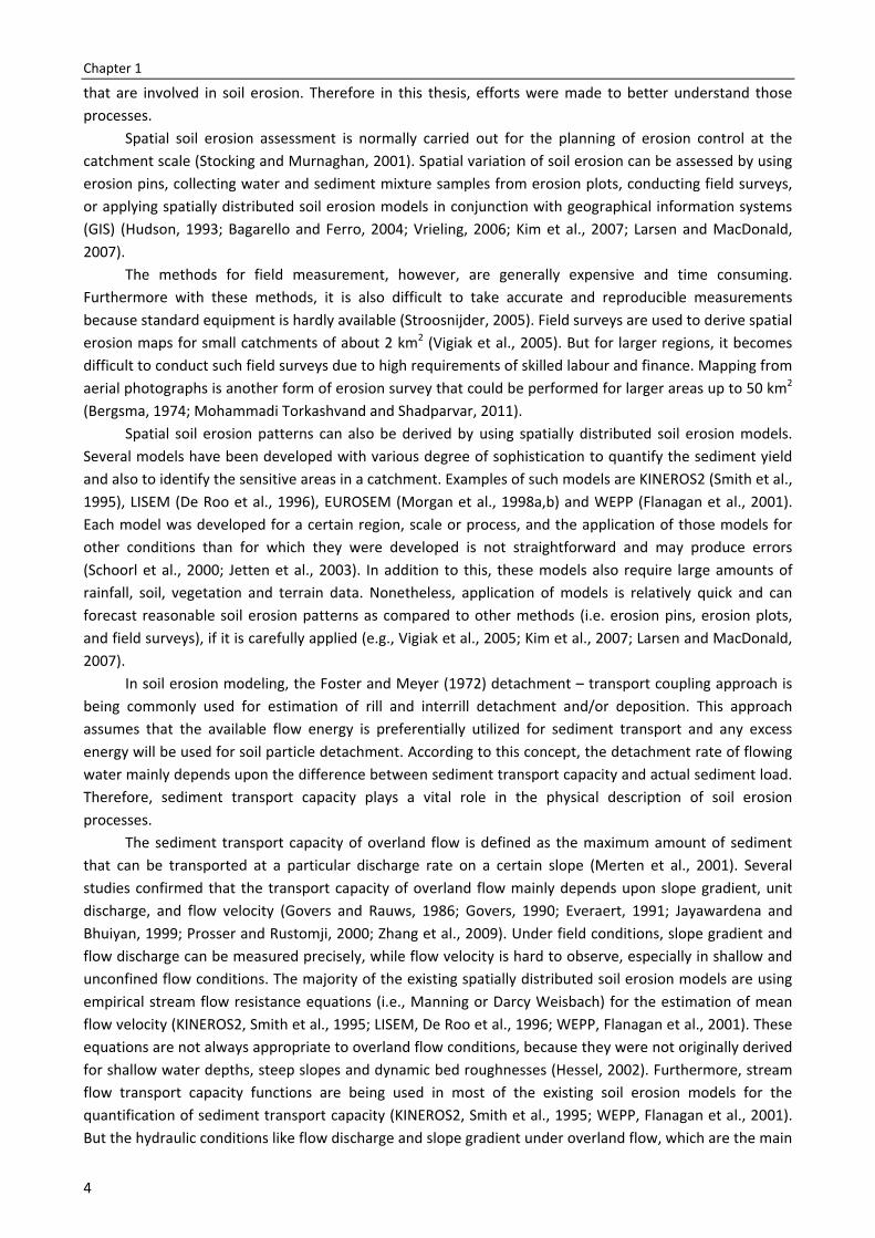
Soil erosion by water remains an important global issue in the 21st century due to its adverse on-site and off-site impacts. On-site impacts of erosion include losses of soil, plant nutrients, organic matter, plant available water and applied fertilizer, which strongly affect the agricultural yield (Lal, 1998; Schoorl et al., 2002). On a global scale, the on-site erosion is reducing the crop productivity by about 33% of the world’s arable lands (Brown and Young, 1990; Lal, 1998; Zuazo and Pleguezuelo, 2008). In-addition, their off-site impacts of erosion include damage to water-based navigation systems, water storage facilities, power generation facilities, and water conveyance systems, as well as increased the risk of flooding (Pimentel et al., 1995; Veldkamp et al., 2001). One of the main off-site impacts of soil erosion includes the loss of water storage capacity of dams due to sedimentation. Worldwide, the average annual loss of storage capacity of reservoirs is roughly 1% corresponding to about 50 km3 (Mahmood, 1987; Sloff, 1997). But some countries may have much higher storage loss of their reservoirs, e.g. the average annual storage depletion rate of reservoirs in China and Turkey is almost 2.3 and 1.5%, respectively, due to low forest cover, barren lands, and steep slopes (Sloff, 1997). In Pakistan, the average annual storage depletion rate of existing reservoirs (i.e. Tarbela and Mangla) is also slightly higher than the global rate (Ali et al., 2006; DBC, 2007), which can be reduced by executing appropriate soil and water conservation practices in the catchments (Minella et al., 2009; Solaimani et al., 2009).
At the catchment scale, the eroded volume of the sediment from hillslopes makes a substantial contribution in total sediment yield, and almost 40% of that material may get deposited into the reservoirs (Plata Bedmar et al., 1997). From a hillslope, soil is mainly eroded in form of splash, interrill and rill erosion. Splash erosion is the removal of sediment particles due to raindrop impact and is assumed to be the first phase of the soil erosion process (Poesen and Savat, 1981; Savat, 1981; Moss and Green, 1983). Splash erosion is not considered in this thesis, because here we deal with detachment and transport of sediment by layers of overland flow only. Interrill or sheet erosion can be defined as the uniform removal of thin layers of soil from a relatively smooth soil surface (Foster and Meyer, 1972; Toy et al., 2002; Acharya et al., 2009). Govers and Poesen (1988) in Belgium, Ludwig et al. (1995) in Northern France, and Rodríguez-Blanco et al. (2010) in NW Spain reported that the contribution of interrill erosion to the total eroded volume of sediment at both field and catchment scales ranges between 10 and 20%.
Under natural conditions, soil erosion processes hardly remain uniform for longer periods, and runoff starts concentrating in small channels (i.e rills) after a very short distance. The resulting channels are usually small and shallow, and can be easily removed by normal tillage practices (Hutchinson and Pritchard, 1976; Loch et al., 1989; Poesen, 1993; Woodward, 1999; Soil Science Society of America, 2001; Martínez-Casasnovas et al., 2005). Rills usually do not reappear in the same place after obliteration by tillage (Foster, 1986; Vandaele and Poesen, 1995; Cerdan et al., 2002). By comparing the contribution of rill and interrill erosion in total soil loss, several studies found that approximately 80% of sediment from hillslopes is eroded due to rill erosion (Moss and Walker, 1978; Fullen and Reed, 1987; Ludwig et al., 1995; Rodríguez-Blanco et al., 2010).
Many watershed management practices are being used to control water erosion from hillslopes. Examples are contour strips of dense vegetation, terraces, flow diversions and armoured waterways for runoff disposal (Toy et al., 2002). Currently the main challenge for scientists is the accurate assessment of erosion problems at the catchment scale (Okoba, 2005). In other words, where are the areas that are most at risk and should be treated, and what are the most appropriate soil and water conservation techniques? In order to precisely identify the sensitive areas in a catchment, it is essential to understand the processes
Chapter 1
4
that are involved in soil erosion. Therefore in this thesis, efforts were made to better understand those processes.
Spatial soil erosion assessment is normally carried out for the planning of erosion control at the catchment scale (Stocking and Murnaghan, 2001). Spatial variation of soil erosion can be assessed by using erosion pins, collecting water and sediment mixture samples from erosion plots, conducting field surveys, or applying spatially distributed soil erosion models in conjunction with geographical information systems (GIS) (Hudson, 1993; Bagarello and Ferro, 2004; Vrieling, 2006; Kim et al., 2007; Larsen and MacDonald, 2007).
The methods for field measurement, however, are generally expensive and time consuming. Furthermore with these methods, it is also difficult to take accurate and reproducible measurements because standard equipment is hardly available (Stroosnijder, 2005). Field surveys are used to derive spatial erosion maps for small catchments of about 2 km2 (Vigiak et al., 2005). But for larger regions, it becomes difficult to conduct such field surveys due to high requirements of skilled labour and finance. Mapping from aerial photographs is another form of erosion survey that could be performed for larger areas up to 50 km2 (Bergsma, 1974; Mohammadi Torkashvand and Shadparvar, 2011).
Spatial soil erosion patterns can also be derived by using spatially distributed soil erosion models. Several models have been developed with various degree of sophistication to quantify the sediment yield and also to identify the sensitive areas in a catchment. Examples of such models are KINEROS2 (Smith et al., 1995), LISEM (De Roo et al., 1996), EUROSEM (Morgan et al., 1998a,b) and WEPP (Flanagan et al., 2001). Each model was developed for a certain region, scale or process, and the application of those models for other conditions than for which they were developed is not straightforward and may produce errors (Schoorl et al., 2000; Jetten et al., 2003). In addition to this, these models also require large amounts of rainfall, soil, vegetation and terrain data. Nonetheless, application of models is relatively quick and can forecast reasonable soil erosion patterns as compared to other methods (i.e. erosion pins, erosion plots, and field surveys), if it is carefully applied (e.g., Vigiak et al., 2005; Kim et al., 2007; Larsen and MacDonald, 2007).
In soil erosion modeling, the Foster and Meyer (1972) detachment – transport coupling approach is being commonly used for estimation of rill and interrill detachment and/or deposition. This approach assumes that the available flow energy is preferentially utilized for sediment transport and any excess energy will be used for soil particle detachment. According to this concept, the detachment rate of flowing water mainly depends upon the difference between sediment transport capacity and actual sediment load. Therefore, sediment transport capacity plays a vital role in the physical description of soil erosion processes.
The sediment transport capacity of overland flow is defined as the maximum amount of sediment that can be transported at a particular discharge rate on a certain slope (Merten et al., 2001). Several studies confirmed that the transport capacity of overland flow mainly depends upon slope gradient, unit discharge, and flow velocity (Govers and Rauws, 1986; Govers, 1990; Everaert, 1991; Jayawardena and Bhuiyan, 1999; Prosser and Rustomji, 2000; Zhang et al., 2009). Under field conditions, slope gradient and flow discharge can be measured precisely, while flow velocity is hard to observe, especially in shallow and unconfined flow conditions. The majority of the existing spatially distributed soil erosion models are using empirical stream flow resistance equations (i.e., Manning or Darcy Weisbach) for the estimation of mean flow velocity (KINEROS2, Smith et al., 1995; LISEM, De Roo et al., 1996; WEPP, Flanagan et al., 2001). These equations are not always appropriate to overland flow conditions, because they were not originally derived for shallow water depths, steep slopes and dynamic bed roughnesses (Hessel, 2002). Furthermore, stream flow transport capacity functions are being used in most of the existing soil erosion models for the quantification of sediment transport capacity (KINEROS2, Smith et al., 1995; WEPP, Flanagan et al., 2001). But the hydraulic conditions like flow discharge and slope gradient under overland flow, which are the main
Introduction
5
driving forces, are entirely different from the conditions in stream flow that make their use debatable (Hessel and Jetten, 2007).
During the last three decades, several studies were carried out to understand the hydraulics of overland flow (e.g., Line and Meyer, 1988; Govers, 1992a,b; Nearing et al., 1997, Takken et al., 1998; Nearing et al., 1999; Takken and Govers, 2000), but research is still needed for the precise estimation of major hydraulic variables of overland flow, such as mean flow velocity, discharge, sediment transport capacity, etc. Many efforts have already been made to better understand the processes involved in transport of sediment under overland flow conditions (e.g. Beasley and Huggins, 1982; Govers and Rauws, 1986; Govers, 1990; Guy et al., 1990; Everaert, 1991; Abrahams and Li, 1998; Prosser and Rustomji, 2000; Abrahams et al., 2001; Zhang et al., 2009; Zhang et al., 2010a,b,c). But, there is still a need to improve the mathematical framework for the estimation of sediment transport capacity of overland flow by considering physical parameters. In order to do so, it is imperative to study the impact of hydraulic parameters like unit discharge, slope gradient and mean flow velocity on sediment transport capacity.
1.2 Research objective, hypothesis and questions
The main objective of the research described in this thesis was to develop an accurate equation for the precise estimation of sediment transport capacity in overland flow conditions. The new equation should be easily applicable to overland flow conditions and depend on those hydraulic and sediment parameters that can be easily measured in the field. The investigations started from the hypothesis, that there is a close relation between sediment transport capacity, flow velocity, discharge and the characteristics of the eroded sediments. Knowing this relationship will enable to quantify sediment transport capacity of overland flows, and such quantification will allow for better soil erosion modeling.
Three research questions were addressed in this thesis to accomplish the above objective: (i) How suitable are the existing approaches and functions that are used for mean flow velocity and
sediment transport capacity quantification under overland flow conditions? (ii) Which hydrological and morphological factors affect and control the mean flow velocity and
sediment transport capacity? (iii) What are optimal functions for the quantification of mean flow velocity and sediment transport
capacity?
1.3 Experimental set-up
During the last several decades, many scientists carried out laboratory flume experiments to improve their understanding of the processes involved in transport of sediments under overland flow conditions (e.g. Emmett, 1970; Govers and Rauws; 1986; Guy et al., 1990; Everaert, 1991; Govers, 1992a,b; Li et al., 1996; Li and Abrahams, 1997; Abrahams and Li, 1998; Nearing et al., 1999; Dunkerley, 2001; Gimenez and Govers, 2002; Zhang et al., 2010a,b,c). Laboratory experimentation allows to have control over initial and boundary conditions, and can simulate the same soil characteristics as encountered under natural conditions to some extent, but with much better accessibility (Black, 1970; Hacking, 1984; Ghodrati et al., 1999; Morgan, 2003; Kleinhans et al., 2010). Furthermore, laboratory experiments reflect the natural conditions at a small scale and led to new theories. In general, laboratory experiments showed great potential to gain understanding of the natural processes involved in soil erosion, and experimental observations can be considered as a simplified but valid representation of the reality (Paola et al., 2009).
For the development of physically-based equations, it is necessary to represent the physical processes by incorporating appropriate parameters into an equation (Kleinhans et al., 2010). But the values
Chapter 1
6
of these parameters are usually poorly known or difficult to measure for field conditions, like flow depth, local flow velocity, etc. (Jayawardena and Bhuiyan, 1999). However, these parameters can be measured in the laboratory at a reasonable accuracy (Raffel et al., 1998; Dunkerley, 2003; Gimenez et al., 2004; Planchon et al., 2005; Lei et al., 2010; Zhang et al., 2010b).
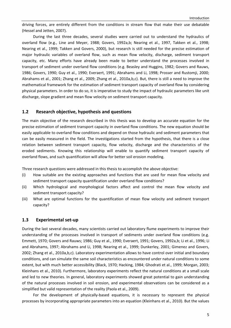
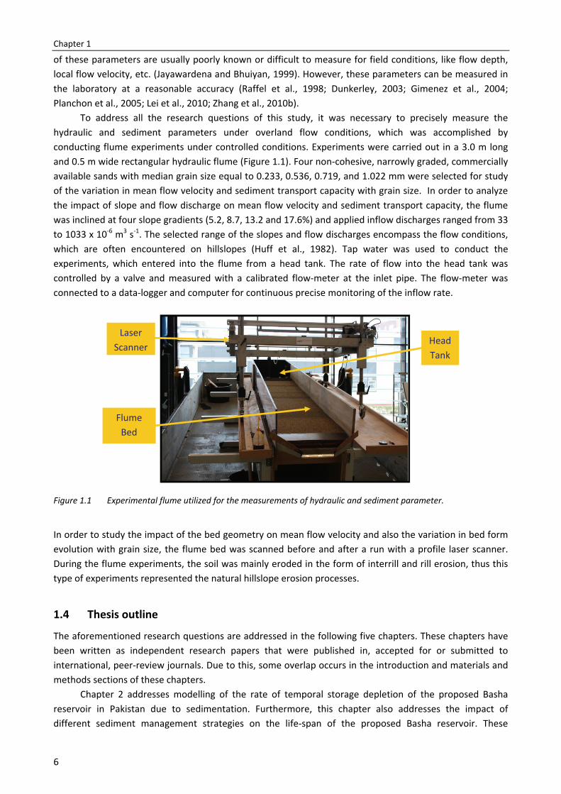
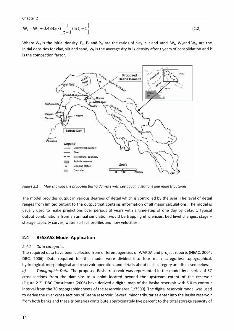
To address all the research questions of this study, it was necessary to precisely measure the hydraulic and sediment parameters under overland flow conditions, which was accomplished by conducting flume experiments under controlled conditions. Experiments were carried out in a 3.0 m long and 0.5 m wide rectangular hydraulic flume (Figure 1.1). Four non-cohesive, narrowly graded, commercially available sands with median grain size equal to 0.233, 0.536, 0.719, and 1.022 mm were selected for study of the variation in mean flow velocity and sediment transport capacity with grain size. In order to analyze the impact of slope and flow discharge on mean flow velocity and sediment transport capacity, the flume was inclined at four slope gradients (5.2, 8.7, 13.2 and 17.6%) and applied inflow discharges ranged from 33 to 1033 x 10-6 m3 s-1. The selected range of the slopes and flow discharges encompass the flow conditions, which are often encountered on hillslopes (Huff et al., 1982). Tap water was used to conduct the experiments, which entered into the flume from a head tank. The rate of flow into the head tank was controlled by a valve and measured with a calibrated flow-meter at the inlet pipe. The flow-meter was connected to a data-logger and computer for continuous precise monitoring of the inflow rate.
Figure 1.1 Experimental flume utilized for the measurements of hydraulic and sediment parameter.
In order to study the impact of the bed geometry on mean flow velocity and also the variation in bed form evolution with grain size, the flume bed was scanned before and after a run with a profile laser scanner. During the flume experiments, the soil was mainly eroded in the form of interrill and rill erosion, thus this type of experiments represented the natural hillslope erosion processes.
1.4 Thesis outline
The aforementioned research questions are addressed in the following five chapters. These chapters have been written as independent research papers that were published in, accepted for or submitted to international, peer-review journals. Due to this, some overlap occurs in the introduction and materials and methods sections of these chapters.
Chapter 2 addresses modelling of the rate of temporal storage depletion of the proposed Basha reservoir in Pakistan due to sedimentation. Furthermore, this chapter also addresses the impact of different sediment management strategies on the life-span of the proposed Basha reservoir. These
Flume Bed
Laser Scanner
Head Tank
Introduction
7
strategies include the raising of Minimum operation Level (MoL), draw-down the MoL (flushing), and controlling the sediment inflows. The results clearly indicate that raising and draw-down of MoL can only add few more years to its life-span. Whereas, the results highlighted that the reservoir life can be extended more than 100 years if the sediment inflow is reduced by implementing river basin management projects in the catchment area. Such projects can be successfully implemented only if the most sensitive erosion areas can precisely be identified through spatial explicit modelling. In order to do so, it is necessary to reduce the uncertainties that are associated with soil erosion modelling.
In chapter 3, the physical basis and application boundaries of the existing sediment detachment and transport capacity functions, which are being widely used for soil erosion modeling, are reviewed and summarized. In this review, the existing detachment and transport capacity functions were described on the basis of four composite force predictors: shear stress, stream power, unit stream power and effective stream power. Moreover in this chapter, the suitability of these functions for overland flow conditions is also discussed on the basis of information available in the literature.
Chapter 4 presents an alternative method to estimate mean flow velocity for overland flow conditions, instead of using a correction factor as part of the dye-tracing technique. The variation of the dye-tracing correction factor with median grain size and slope gradient was studied in-detail. Given the fact that an absolute value of such correction factor is not applicable to all hydraulic and sedimentary conditions of overland flow (Chapter 4), regression analysis was carried out to examine the impact of different hydraulic and sediment parameters i.e. flow discharge, slope gradient, and median grain size on mean flow velocity. The chapter also addresses the variation of mean flow velocity with micro topography for different sands under similar hydraulic conditions using the data obtained from a laser profile scanner. A relationship was derived on the basis of the data obtained from the flume experiments, in order to precisely predict the mean flow velocity under overland flow conditions.
The information obtained from the laser scanner was used to confirm the hypothesis that a flume length of 3.0 m is sufficient to reach the sediment transport capacity for the given conditions of flow discharge, slope gradient and sediment type. In Chapter 5, the effect of different hydraulic parameters, i.e. unit flow discharge, mean flow velocity and slope gradient on sediment transport capacity for erodible beds is discussed. The aim was to better understand the processes entailed in sediment transport. The results obtained in this chapter for erodible beds were compared with results reported in the literature, which were mainly collected for non-erodible beds. In-addition to this, the ability of composite force predictors (i.e. shear stress, stream power, unit stream power and effective stream power) to predict transport capacity was evaluated, and the dependency of their relation with sediment transport capacity on bed geometry is also discussed.
In chapter 6, the performance of the most well-known and widely used sediment transport capacity functions is evaluated using the results from the experimental flume. Overall, the selected sediment transport capacity functions did not give accurate results and therefore a new sediment transport capacity function was derived by dimensional analysis using unit stream power concept for shallow flows. Finally, the major conclusions of this thesis are discussed in chapter 7 and general directions for future work are also given.

Chapter 2
Evaluation of sediment management strategies on reservoir storage depletion rate: a case study
Ali M. and G. Sterk Journal of Hydraulic, Coastal and Environmental Engineering 66: 207 – 216 (2010)

11
Evaluation of sediment management strategies on reservoir storage depletion rate: as case study
Abstract
Sedimentation aspects have a major role during the design of new reservoir projects because life of the reservoir mainly depends upon sediment handling during reservoir operation. Therefore, proper sediment management strategies should be adopted to enhance the life span of reservoirs. Basha Reservoir is one of the mega water resources projects which are being planned to construct on the Indus river. Under this study, the efficiency of four sediment management strategies were evaluated by using the RESSASS model. The reservoir management strategies considered for sediment simulation of Basha reservoir include the normal operation, raising of MoL, draw-down the MoL (flushing) and controlling the sediment inflows. Under normal operation, the model predicted the life span of Basha reservoir around 55 – 60 years. But by raising of Mol 2.0 m yr-1 implemented after 35 years of operation may add 10 – 15 years more to the life-span of the reservoir. However, by adopting the flushing operation to draw-down the MoL at El. 1010 m initiated after 35 years of operation, it may also add about 15 – 20 years more. Moreover, the results obtained by considering 50% reduction in sediment inflow due to implementation of river basin management projects upstream of Basha within 30 years of reservoir operation, depicts that the life of the reservoir will be more than 100 years. It is therefore concluded that proper sediment mitigation measure can significantly enhance the life-span of planned reservoirs.
2.1 Introduction
Irrigated agriculture is the backbone of Pakistan’s economy (World Bank, 1994). The agricultural sector in Pakistan is mainly relying on water supplies from reservoirs. But irrigated agriculture is seriously confronted with major problems of water scarcity, unequal distribution of irrigation water, low productivity and increasing soil salinity (Tahir and Habib, 2000). The country is already facing a serious shortage of food due to fastly growing population and lack of sizeable water storage (Pakistan Water Partnership, 2001). With the present rate of population growth and reduction of water availability due to siltation of existing reservoirs, Pakistan is likely to reach the stage of “water short country” by the year 2012 when the per capita surface water availability will be reduced to 1000 cubic meter per year (Farooqi, 2006). Rising pressure to produce more food with less water demands not only for the efficient and integrated use of available water resources but also demands the construction of new water reservoirs.
The two existing reservoirs in Pakistan, Tarbela and Mangla are rapidly losing their storage capacities due to sedimentation. The gross storage capacities of Tarbela and Mangla reservoirs at the time of first impoundment were 13.938 and 7.253 BCM respectively. These reservoirs collectively lost about 25% of their storage capacity by the end of the year 2003 (Ali et al., 2006). The hydrographic survey of 2000 showed that the Mangla dam had lost about 20% of its gross storage capacity (Ali et al., 2006). According to the hydrographic survey of 2005, Tarbela dam had lost about 30% of its gross storage capacity (DBC, 2007). It is generally known that the annual loss of storage in reservoirs is roughly 1% corresponding to about 50 km3 world-wide (Mahmood, 1987). But some reservoirs may have much higher storage loss, e.g., the Sanmenxia Reservoir in China looses about 1.7% annually (Sloff, 1997).
In order to meet the growing requirement of water in the country, the Government of Pakistan (GoP) through the Water and Power Development Authority (WAPDA) plans to construct some mega water resources projects in additions to small and medium storage projects on the Indus river. Basha reservoir is
Chapter 2
12
one of the mega water resources projects which are planned on the Indus river. The proposed Basha reservoir will be located 315 Km upstream of Tarbela reservoir. But without any mitigation measures, the viability of existing and planned reservoirs will become questionable under the current high storage depletion rates. Therefore it is essential that proper attention should be paid to sedimentation aspects in the management of the existing reservoirs as well as in the design of new reservoirs. If proper sediment mitigation measures are adopted, life of the reservoir could be extended for a much longer time.
The reservoir depletion rate can be minimized in two different ways i.e. by controlling the sediment inflow rate to the reservoir or by adopting different reservoir operation strategies. The sediment inflow rate can be controlled by adopting sediment management practices in the upstream catchment area (Huang and Zhang, 2004). Nevertheless, two reservoir operation strategies are being commonly used globally for sediment management in reservoirs to conserve the storage capacity and keep the power-intakes free from sediment i.e., draw-down the minimum operation level (flushing) and raising of the minimum operation level. Flushing is one of the most economic methods that partly recovers the depleted storage without dredging or other mechanical means of removing sediment. The success of flushing may depend upon the catchment and reservoir characteristics (White, 2000). Qian (1982) also argued that the flushing solution is only suitable in reservoirs where annually an excess amount of water is available. For the Tarbela reservoir, the raising of Minimum operation Level (MoL) sediment management strategy has been adopted to reduce the speed of delta movement towards the dam body (TAMS, 1998).
Several one-dimensional numerical models are being globally used for reservoir sediment simulation e.g., RESSASS (Wallingford, 2001), HEC-6 (US Army Corps of Engineers, 1992), GSTAR (Yang et al., 2004), Fluvial (Chang et al., 1996). These models have been used as a tool to predict the storage capacity losses and reservoir bed levels after a certain specified simulation period due to sedimentation. RESSASS is a one-dimensional model which was developed by HR-Wallingford, UK, in 1995 to simulate a long-term average pattern of scour and deposition in reservoirs. The model input includes geometrical, hydrological and morphological data. The model output describes the flow velocities, water surface profile, trapping efficiency, storage depletion rate and reservoir bed levels. In this study, the RESSASS model was used for simulation of the sediment dynamics in the proposed Basha Reservoir. The main aim of this study was to investigate the effects of different reservoir operation strategies on the expected life-time of the planned Basha reservoir.
2.2 The Study Area
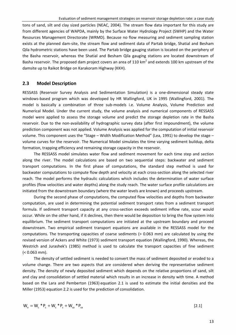
The planned Basha damsite is located about 315 km upstream of Tarbela Dam on the Indus river and 165 km downstream of the Northern Area capital Gilgit and 40 km downstream of Chilas town. The proposed dam is designed for a maximum height of 260 m (NEAC, 2004). The total drainage area of the Indus river above the damsite is 153,200 km2, which extends from Pakistan into Tibet and Kashmir. The major tributaries that join the Indus river above the proposed damsite include the Hunza river, the Gilgit river, the Astore river and the Shyok river (Figure 2.1). The sub-basins formed by these tributaries have distinct morphologic, climatic and hydrologic characteristics. Poor vegetal cover, steep slopes, and the fact that the soils and rocks of the Indus valley are geologically young and easily erodible are some relevant features of the drainage basin responsible for high sediment concentration in the water of the Indus river at the proposed damsite (Sloff, 1997).
The Basha reservoir with full reservoir level (FRL) at El. 1160 m will have a gross storage volume of 10.008 BCM and a dead storage level (MoL) at El. 1060 m with dead storage volume of 2.10 BCM. Two power-houses are planned at El. 1040 m, one on each side of the main dam with total installed power generation capacity of 4500 MW and low-level outlets are planned at El. 975 m (NEAC, 2004). The mean annual unregulated flow of the Indus river at the damsite is 61.12 BCM that carries about 199.40 million
Evaluation of sediment management strategies on reservoir storage depletion rate: a case study
13
tons of sand, silt and clay sized particles (NEAC, 2004). The stream flow data important for this study are from different agencies of WAPDA, mainly by the Surface Water Hydrology Project (SWHP) and the Water Resources Management Directorate (WRMD). Because no flow measuring and sediment sampling station exists at the planned dam-site, the stream flow and sediment data of Partab bridge, Shatial and Besham Qila hydrometric stations have been used. The Partab bridge gauging station is located on the periphery of the Basha reservoir, whereas the Shatial and Besham Qila gauging stations are located downstream of Basha reservoir. The proposed dam project covers an area of 110 km2 and extends 100 km upstream of the damsite up to Raikot Bridge on Karakoram Highway (KKH).
2.3 Model Description
RESSASS (Reservoir Survey Analysis and Sedimentation Simulation) is a one-dimensional steady state windows-based program which was developed by HR Wallingford, UK in 1995 (Wallingford, 2001). The model is basically a combination of three sub-models i.e. Volume Analysis, Volume Prediction and Numerical Model. Under the current study, the volume analysis and numerical components of RESSASS model were applied to assess the storage volume and predict the storage depletion rate in the Basha reservoir. Due to the non-availability of hydrographic survey data (after first impoundment), the volume prediction component was not applied. Volume Analysis was applied for the computation of initial reservoir volume. This component uses the “Stage – Width Modification Method” (Lea, 1991) to develop the stage – volume curves for the reservoir. The Numerical Model simulates the time varying sediment buildup, delta formation, trapping efficiency and remaining storage capacity in the reservoir.
The RESSASS model simulates water flow and sediment movement for each time step and section along the river. The model calculations are based on two sequential steps: backwater and sediment transport computations. In the first phase of computations, the standard step method is used for backwater computations to compute flow depth and velocity at each cross-section along the selected river reach. The model performs the hydraulic calculations which includes the determination of water surface profiles (flow velocities and water depths) along the study reach. The water surface profile calculations are initiated from the downstream boundary (where the water levels are known) and proceeds upstream.
During the second phase of computations, the computed flow velocities and depths from backwater computation, are used in determining the potential sediment transport rates from a sediment transport formula. If sediment transport capacity at any cross-section exceeds sediment inflow rate, scour would occur. While on the other hand, if it declines, then there would be deposition to bring the flow system into equilibrium. The sediment transport computations are initiated at the upstream boundary and proceed downstream. Two empirical sediment transport equations are available in the RESSASS model for the computations. The transporting capacities of coarse sediments (> 0.063 mm) are calculated by using the revised version of Ackers and White (1973) sediment transport equation (Wallingford, 1990). Whereas, the Westrich and Jurashek's (1985) method is used to calculate the transport capacities of fine sediment (< 0.063 mm).
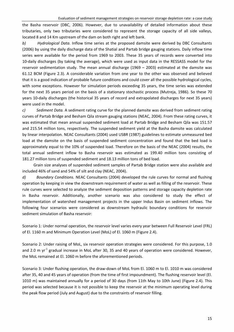
The density of settled sediment is needed to convert the mass of sediment deposited or eroded to a volume change. There are two aspects that are considered when deriving the representative sediment density. The density of newly deposited sediment which depends on the relative proportions of sand, silt and clay and consolidation of settled material which results in an increase in density with time. A method based on the Lara and Pemberton (1963) equation 2.1 is used to estimate the initial densities and the Miller (1953) equation 2.2 is used for the prediction of consolidation.
sasasscco P*WP*WP*WW ++= [2.1]
Chapter 2
14
−
−+= 1)t(ln
1tt)k(4343.0WW ot [2.2]
Where W0 is the initial density, Pc, Ps and Psa are the ratios of clay, silt and sand, Wc, Ws and Wsa are the initial densities for clay, silt and sand, Wt is the average dry bulk density after t years of consolidation and k is the compaction factor.
Figure 2.1 Map showing the proposed Basha damsite with key gauging stations and main tributaries.
The model provides output in various degrees of detail which is controlled by the user. The level of detail ranges from limited output to the output that contains information of all major calculations. The model is usually used to make predictions over periods of years with a time-step of one day by default. Typical output combinations from an annual simulation would be trapping efficiencies, bed level changes, stage – storage capacity curves, water surface profiles and flow velocities.
2.4 RESSASS Model Application
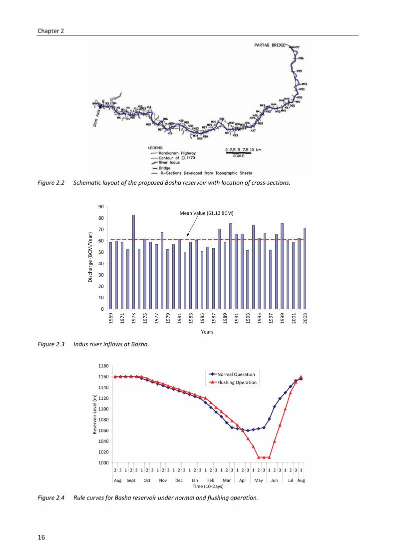
2.4.1 Data categories The required data have been collected from different agencies of WAPDA and project reports (NEAC, 2004; DBC, 2006). Data required for the model were divided into four main categories; topographical, hydrological, morphological and reservoir operation, and details about each category are discussed below: a) Topographic Data. The proposed Basha reservoir was represented in the model by a series of 57 cross-sections from the dam-site to a point located beyond the upstream extent of the reservoir (Figure 2.2). DBC Consultants (2006) have derived a digital map of the Basha reservoir with 5.0 m contour interval from the 70 topographic sheets of the reservoir area (1:7500). The digital reservoir model was used to derive the river cross-sections of Basha reservoir. Several minor tributaries enter into the Basha reservoir from both banks and these tributaries contribute approximately five percent to the total storage capacity of
Evaluation of sediment management strategies on reservoir storage depletion rate: a case study
15
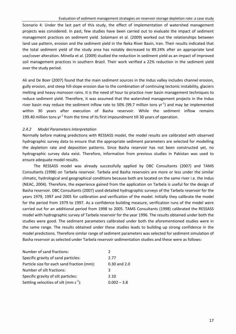
the Basha reservoir (DBC, 2006). However, due to unavailability of detailed information about these tributaries, only two tributaries were considered to represent the storage capacity of all side valleys, located 8 and 14 Km upstream of the dam on both right and left bank. b) Hydrological Data. Inflow time series at the proposed damsite were derived by DBC Consultants (2006) by using the daily discharge data of the Shatial and Partab bridge gauging stations. Daily inflow time series were available for the period from 1969 to 2003. These 35 years of records were converted into 10-daily discharges (by taking the average), which were used as input data in the RESSASS model for the reservoir sedimentation study. The mean annual discharge (1969 – 2003) estimated at the damsite was 61.12 BCM (Figure 2.3). A considerable variation from one year to the other was observed and believed that it is a good indication of probable future conditions and could cover all the possible hydrological cycles, with some exceptions. However for simulation periods exceeding 35 years, the time series was extended for the next 35 years period on the basis of a stationary stochastic process (Mutreja, 1986). So these 70 years 10-daily discharges (the historical 35 years of record and extrapolated discharges for next 35 years) were used in the model. c) Sediment Data. A sediment rating curve for the planned damsite was derived from sediment rating curves of Partab Bridge and Besham Qila stream gauging stations (NEAC, 2004). From these rating curves, it was estimated that mean annual suspended sediment load at Partab Bridge and Besham Qila was 151.57 and 215.54 million tons, respectively. The suspended sediment yield at the Basha damsite was calculated by linear interpolation. NEAC Consultants (2004) used USBR (1987) guidelines to estimate unmeasured bed load at the damsite on the basis of suspended sediment concentration and found that the bed load is approximately equal to the 10% of suspended load. Therefore on the basis of the NEAC (2004) results, the total annual sediment inflow to Basha reservoir was estimated as 199.40 million tons consisting of 181.27 million tons of suspended sediment and 18.13 million tons of bed load.
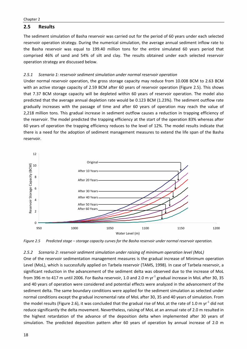
Grain size analyses of suspended sediment samples of Partab Bridge station were also available and included 46% of sand and 54% of silt and clay (NEAC, 2004). d) Boundary Conditions. NEAC Consultants (2004) developed the rule curves for normal and flushing operation by keeping in view the downstream requirement of water as well as filling of the reservoir. These rule curves were selected to analyze the sediment deposition patterns and storage capacity depletion rate in Basha reservoir. Additionally, another scenario was also considered to study the effect of implementation of watershed management projects in the upper Indus Basin on sediment inflows. The following four scenarios were considered as downstream hydraulic boundary conditions for reservoir sediment simulation of Basha reservoir: Scenario 1: Under normal operation, the reservoir level varies every year between Full Reservoir Level (FRL) of El. 1160 m and Minimum Operation Level (MoL) of El. 1060 m (Figure 2.4). Scenario 2: Under raising of MoL, six reservoir operation strategies were considered. For this purpose, 1.0 and 2.0 m yr-1 gradual increase in MoL after 30, 35 and 40 years of operation were considered. However, the MoL remained at El. 1060 m before the aforementioned periods. Scenario 3: Under flushing operation, the draw-down of MoL from El. 1060 m to El. 1010 m was considered after 35, 40 and 45 years of operation (from the time of first impoundment). The flushing reservoir level (El. 1010 m) was maintained annually for a period of 30 days (from 11th May to 10th June) (Figure 2.4). This period was selected because it is not possible to keep the reservoir at the minimum operating level during the peak flow period (July and August) due to the constraints of reservoir filling.
Chapter 2
16
Figure 2.2 Schematic layout of the proposed Basha reservoir with location of cross-sections.
Figure 2.3 Indus river inflows at Basha.
Figure 2.4 Rule curves for Basha reservoir under normal and flushing operation.
0
10
20
30
40
50
60
70
80
90
1969
1971
1973
1975
1977
1979
1981
1983
1985
1987
1989
1991
1993
1995
1997
1999
2001
2003
Years
Disc
harg
e (B
CM/Y
ear)
Mean Value (61.12 BCM)
1000
1020
1040
1060
1080
1100
1120
1140
1160
1180
2 3 1 2 3 1 2 3 1 2 3 1 2 3 1 2 3 1 2 3 1 2 3 1 2 3 1 2 3 1 2 3 1 2 3 1
Aug Sept Oct Nov Dec Jan Feb Mar Apr May Jun Jul AugTime (10-Days)
Rese
rvoi
r Lev
el (m
)
Normal OperationFlushing Operation
Evaluation of sediment management strategies on reservoir storage depletion rate: a case study
17
Scenario 4: Under the last part of this study, the effect of implementation of watershed management projects was considered. In past, few studies have been carried out to evaluate the impact of sediment management practices on sediment yield. Solaimani et al. (2009) worked out the relationships between land use pattern, erosion and the sediment yield in the Neka River Basin, Iran. Their results indicated that the total sediment yield of the study area has notably decreased to 89.24% after an appropriate land use/cover alteration. Minella et al. (2009) studied the reduction in sediment yield as an impact of improved soil management practices in southern Brazil. Their work verified a 22% reduction in the sediment yield over the study period. Ali and De Boer (2007) found that the main sediment sources in the Indus valley includes channel erosion, gully erosion, and steep hill-slope erosion due to the combination of continuing tectonic instability, glaciers melting and heavy monsoon rains. It is the need of hour to practice river basin management techniques to reduce sediment yield. Therefore, it was assumed that the watershed management projects in the Indus river basin may reduce the sediment inflow rate to 50% (99.7 million tons yr-1) and may be implemented within 30 years after execution of Basha reservoir. While the sediment inflow remains 199.40 million tons yr-1 from the time of its first impoundment till 30 years of operation.
2.4.2 Model Parameters Interpretation Normally before making predictions with RESSASS model, the model results are calibrated with observed hydrographic survey data to ensure that the appropriate sediment parameters are selected for modelling the depletion rate and deposition patterns. Since Basha reservoir has not been constructed yet, no hydrographic survey data exist. Therefore, information from previous studies in Pakistan was used to ensure adequate model results.
The RESSASS model was already successfully applied by DBC Consultants (2007) and TAMS Consultants (1998) on Tarbela reservoir. Tarbela and Basha reservoirs are more or less under the similar climatic, hydrological and geographical conditions because both are located on the same river i.e. the Indus (NEAC, 2004). Therefore, the experience gained from the application on Tarbela is useful for the design of Basha reservoir. DBC Consultants (2007) used detailed hydrographic surveys of the Tarbela reservoir for the years 1979, 1997 and 2005 for calibration and verification of the model. Initially they calibrate the model for the period from 1979 to 1997. As a confidence building measure, verification runs of the model were carried out for an additional period from 1998 to 2005. TAMS Consultants (1998) calibrated the RESSASS model with hydrographic survey of Tarbela reservoir for the year 1996. The results obtained under both the studies were good. The sediment parameters calibrated under both the aforementioned studies were in the same range. The results obtained under these studies leads to building up strong confidence in the model predictions. Therefore similar range of sediment parameters was selected for sediment simulation of Basha reservoir as selected under Tarbela reservoir sedimentation studies and these were as follows:
Number of sand fractions: 2 Specific gravity of sand particles: 2.77 Particle size for each sand fraction (mm): 0.30 and 2.0 Number of silt fractions: 3 Specific gravity of silt particles: 2.10 Settling velocities of silt (mm s-1): 0.002 – 3.8
Chapter 2
18
2.5 Results
The sediment simulation of Basha reservoir was carried out for the period of 60 years under each selected reservoir operation strategy. During the numerical simulation, the average annual sediment inflow rate to the Basha reservoir was equal to 199.40 million tons for the entire simulated 60 years period that comprised 46% of sand and 54% of silt and clay. The results obtained under each selected reservoir operation strategy are discussed below.
2.5.1 Scenario 1: reservoir sediment simulation under normal reservoir operation Under normal reservoir operation, the gross storage capacity may reduce from 10.008 BCM to 2.63 BCM with an active storage capacity of 2.59 BCM after 60 years of reservoir operation (Figure 2.5). This shows that 7.37 BCM storage capacity will be depleted within 60 years of reservoir operation. The model also predicted that the average annual depletion rate would be 0.123 BCM (1.23%). The sediment outflow rate gradually increases with the passage of time and after 60 years of operation may reach the value of 2,218 million tons. This gradual increase in sediment outflow causes a reduction in trapping efficiency of the reservoir. The model predicted the trapping efficiency at the start of the operation 83% whereas after 60 years of operation the trapping efficiency reduces to the level of 12%. The model results indicate that there is a need for the adoption of sediment management measures to extend the life span of the Basha reservoir.
Figure 2.5 Predicted stage – storage capacity curves for the Basha reservoir under normal reservoir operation.
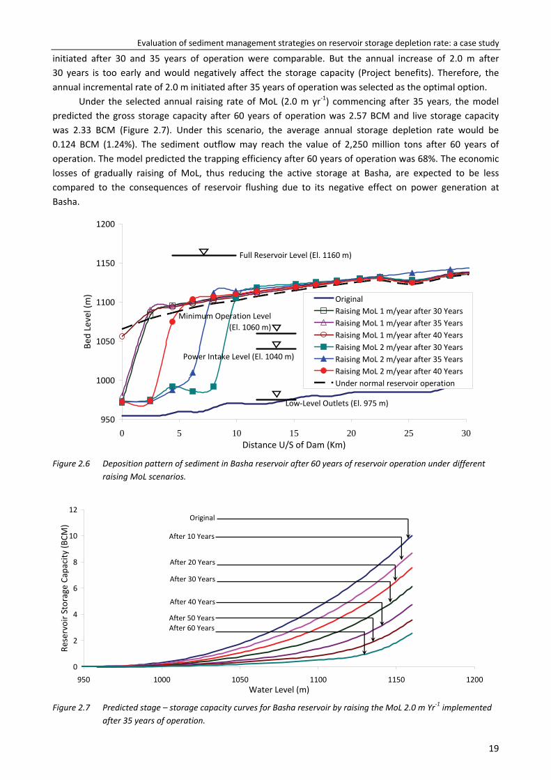
2.5.2 Scenario 2: reservoir sediment simulation under raising of minimum operation level (MoL) One of the reservoir sedimentation management measures is the gradual increase of Minimum operation Level (MoL), which is successfully applied on Tarbela reservoir (TAMS, 1998). In case of Tarbela reservoir, a significant reduction in the advancement of the sediment delta was observed due to the increase of MoL from 396 m to 417 m until 2006. For Basha reservoir, 1.0 and 2.0 m yr-1 gradual increase in MoL after 30, 35 and 40 years of operation were considered and potential effects were analyzed in the advancement of the sediment delta. The same boundary conditions were applied for the sediment simulation as selected under normal conditions except the gradual incremental rate of MoL after 30, 35 and 40 years of simulation. From the model results (Figure 2.6), it was concluded that the gradual rise of MoL at the rate of 1.0 m yr-1 did not reduce significantly the delta movement. Nevertheless, raising of MoL at an annual rate of 2.0 m resulted in the highest retardation of the advance of the deposition delta when implemented after 30 years of simulation. The predicted deposition pattern after 60 years of operation by annual increase of 2.0 m
0
2
4
6
8
10
12
950 1000 1050 1100 1150 1200Water Level (m)
Rese
rvoi
r Sto
rage
Cap
acity
(BCM
) Original
After 10 Years
After 20 Years
After 30 Years
After 40 Years
After 50 YearsAfter 60 Years
Evaluation of sediment management strategies on reservoir storage depletion rate: a case study
19
initiated after 30 and 35 years of operation were comparable. But the annual increase of 2.0 m after 30 years is too early and would negatively affect the storage capacity (Project benefits). Therefore, the annual incremental rate of 2.0 m initiated after 35 years of operation was selected as the optimal option.
Under the selected annual raising rate of MoL (2.0 m yr-1) commencing after 35 years, the model predicted the gross storage capacity after 60 years of operation was 2.57 BCM and live storage capacity was 2.33 BCM (Figure 2.7). Under this scenario, the average annual storage depletion rate would be 0.124 BCM (1.24%). The sediment outflow may reach the value of 2,250 million tons after 60 years of operation. The model predicted the trapping efficiency after 60 years of operation was 68%. The economic losses of gradually raising of MoL, thus reducing the active storage at Basha, are expected to be less compared to the consequences of reservoir flushing due to its negative effect on power generation at Basha.
Figure 2.6 Deposition pattern of sediment in Basha reservoir after 60 years of reservoir operation under different raising MoL scenarios.
Figure 2.7 Predicted stage – storage capacity curves for Basha reservoir by raising the MoL 2.0 m Yr-1 implemented after 35 years of operation.
950
1000
1050
1100
1150
1200
0 5 10 15 20 25 30Distance U/S of Dam (Km)
Bed
Leve
l (m
) OriginalRaising MoL 1 m/year after 30 YearsRaising MoL 1 m/year after 35 YearsRaising MoL 1 m/year after 40 YearsRaising MoL 2 m/year after 30 YearsRaising MoL 2 m/year after 35 YearsRaising MoL 2 m/year after 40 YearsUnder normal reservoir operation
Minimum Operation Level(El. 1060 m)
Low-Level Outlets (El. 975 m)
Power Intake Level (El. 1040 m)
Full Reservoir Level (El. 1160 m)
0
2
4
6
8
10
12
950 1000 1050 1100 1150 1200Water Level (m)
Rese
rvoi
r Sto
rage
Cap
acity
(BCM
)
Original
After 10 Years
After 20 Years
After 30 Years
After 40 Years
After 50 YearsAfter 60 Years
Chapter 2
20
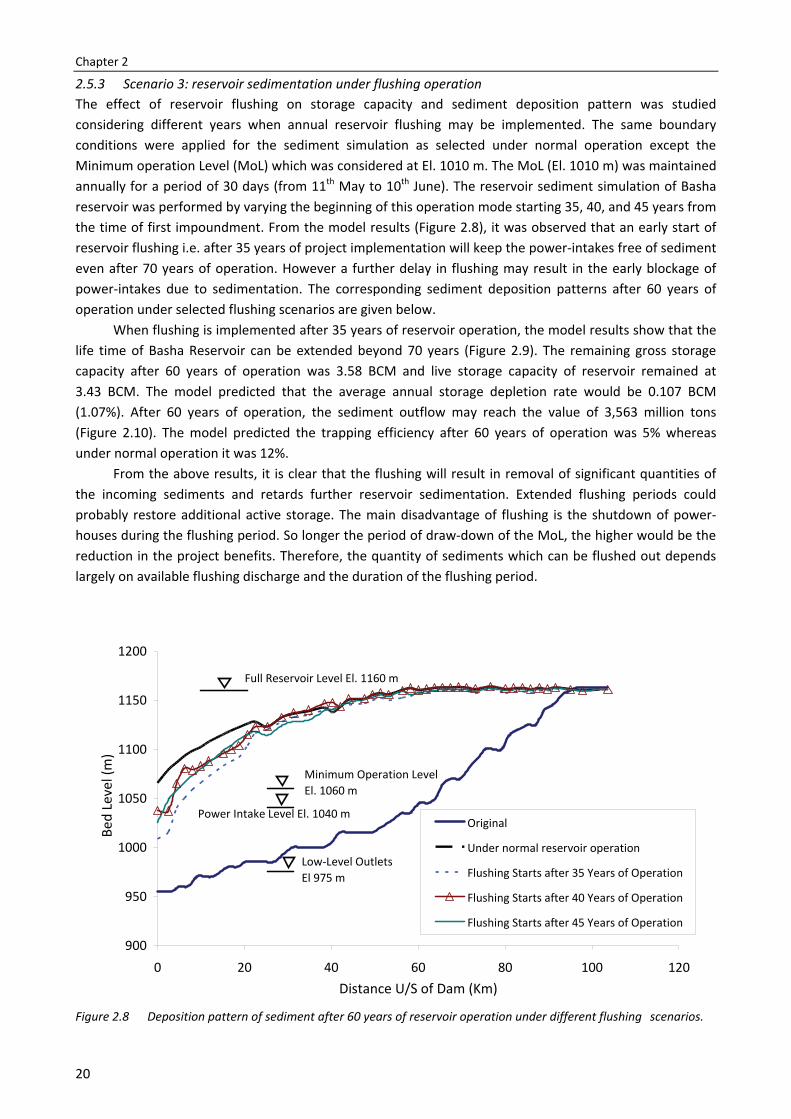
2.5.3 Scenario 3: reservoir sedimentation under flushing operation The effect of reservoir flushing on storage capacity and sediment deposition pattern was studied considering different years when annual reservoir flushing may be implemented. The same boundary conditions were applied for the sediment simulation as selected under normal operation except the Minimum operation Level (MoL) which was considered at El. 1010 m. The MoL (El. 1010 m) was maintained annually for a period of 30 days (from 11th May to 10th June). The reservoir sediment simulation of Basha reservoir was performed by varying the beginning of this operation mode starting 35, 40, and 45 years from the time of first impoundment. From the model results (Figure 2.8), it was observed that an early start of reservoir flushing i.e. after 35 years of project implementation will keep the power-intakes free of sediment even after 70 years of operation. However a further delay in flushing may result in the early blockage of power-intakes due to sedimentation. The corresponding sediment deposition patterns after 60 years of operation under selected flushing scenarios are given below.
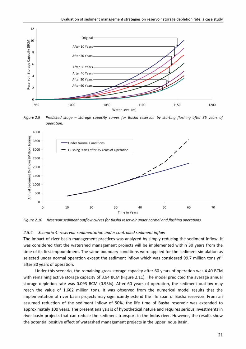
When flushing is implemented after 35 years of reservoir operation, the model results show that the life time of Basha Reservoir can be extended beyond 70 years (Figure 2.9). The remaining gross storage capacity after 60 years of operation was 3.58 BCM and live storage capacity of reservoir remained at 3.43 BCM. The model predicted that the average annual storage depletion rate would be 0.107 BCM (1.07%). After 60 years of operation, the sediment outflow may reach the value of 3,563 million tons (Figure 2.10). The model predicted the trapping efficiency after 60 years of operation was 5% whereas under normal operation it was 12%.
From the above results, it is clear that the flushing will result in removal of significant quantities of the incoming sediments and retards further reservoir sedimentation. Extended flushing periods could probably restore additional active storage. The main disadvantage of flushing is the shutdown of power-houses during the flushing period. So longer the period of draw-down of the MoL, the higher would be the reduction in the project benefits. Therefore, the quantity of sediments which can be flushed out depends largely on available flushing discharge and the duration of the flushing period.
Figure 2.8 Deposition pattern of sediment after 60 years of reservoir operation under different flushing scenarios.
900
950
1000
1050
1100
1150
1200
0 20 40 60 80 100 120Distance U/S of Dam (Km)
Bed
Leve
l (m
)
Original
Under normal reservoir operation
Flushing Starts after 35 Years of Operation
Flushing Starts after 40 Years of Operation
Flushing Starts after 45 Years of Operation
Full Reservoir Level El. 1160 m
Minimum Operation Level El. 1060 m
Low-Level OutletsEl 975 m
Power Intake Level El. 1040 m
Evaluation of sediment management strategies on reservoir storage depletion rate: a case study
21
Figure 2.9 Predicted stage – storage capacity curves for Basha reservoir by starting flushing after 35 years of
operation.
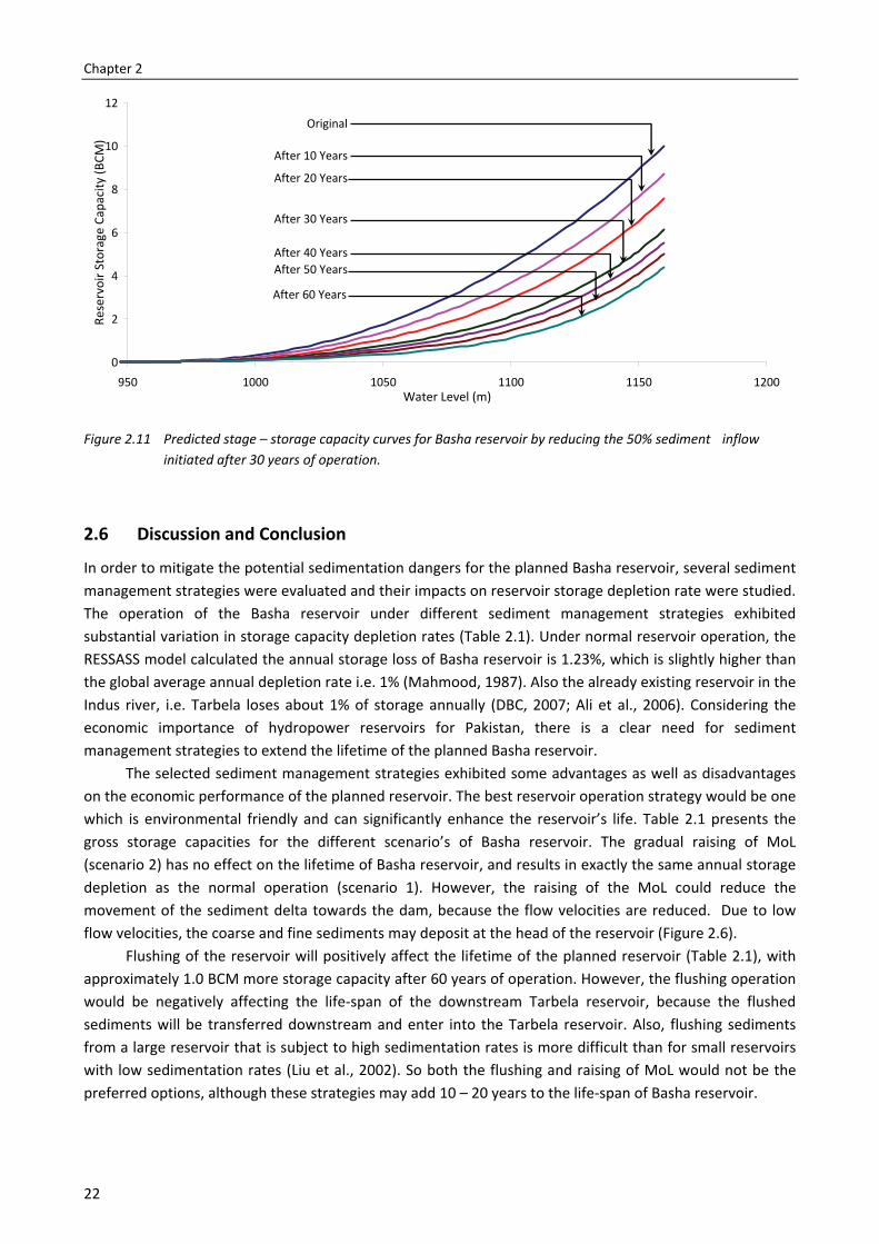
Figure 2.10 Reservoir sediment outflow curves for Basha reservoir under normal and flushing operations. 2.5.4 Scenario 4: reservoir sedimentation under controlled sediment inflow The impact of river basin management practices was analyzed by simply reducing the sediment inflow. It was considered that the watershed management projects will be implemented within 30 years from the time of its first impoundment. The same boundary conditions were applied for the sediment simulation as selected under normal operation except the sediment inflow which was considered 99.7 million tons yr-1 after 30 years of operation.
Under this scenario, the remaining gross storage capacity after 60 years of operation was 4.40 BCM with remaining active storage capacity of 3.94 BCM (Figure 2.11). The model predicted the average annual storage depletion rate was 0.093 BCM (0.93%). After 60 years of operation, the sediment outflow may reach the value of 1,602 million tons. It was observed from the numerical model results that the implementation of river basin projects may significantly extend the life span of Basha reservoir. From an assumed reduction of the sediment inflow of 50%, the life time of Basha reservoir was extended to approximately 100 years. The present analysis is of hypothetical nature and requires serious investments in river basin projects that can reduce the sediment transport in the Indus river. However, the results show the potential positive effect of watershed management projects in the upper Indus Basin.
0
2
4
6
8
10
12
950 1000 1050 1100 1150 1200Water Level (m)
Rese
rvoi
r Sto
rage
Cap
acity
(BCM
) Original
After 10 Years
After 20 Years
After 30 Years
After 40 Years
After 50 Years
After 60 Years
0
500
1000
1500
2000
2500
3000
3500
4000
0 10 20 30 40 50 60 70Time in Years
Annu
al S
edim
ent O
utflo
ws (
Mill
ion
Tonn
es)
Under Normal Conditions
Flushing Starts after 35 Years of Operation
Chapter 2
22
Figure 2.11 Predicted stage – storage capacity curves for Basha reservoir by reducing the 50% sediment inflow initiated after 30 years of operation.
2.6 Discussion and Conclusion
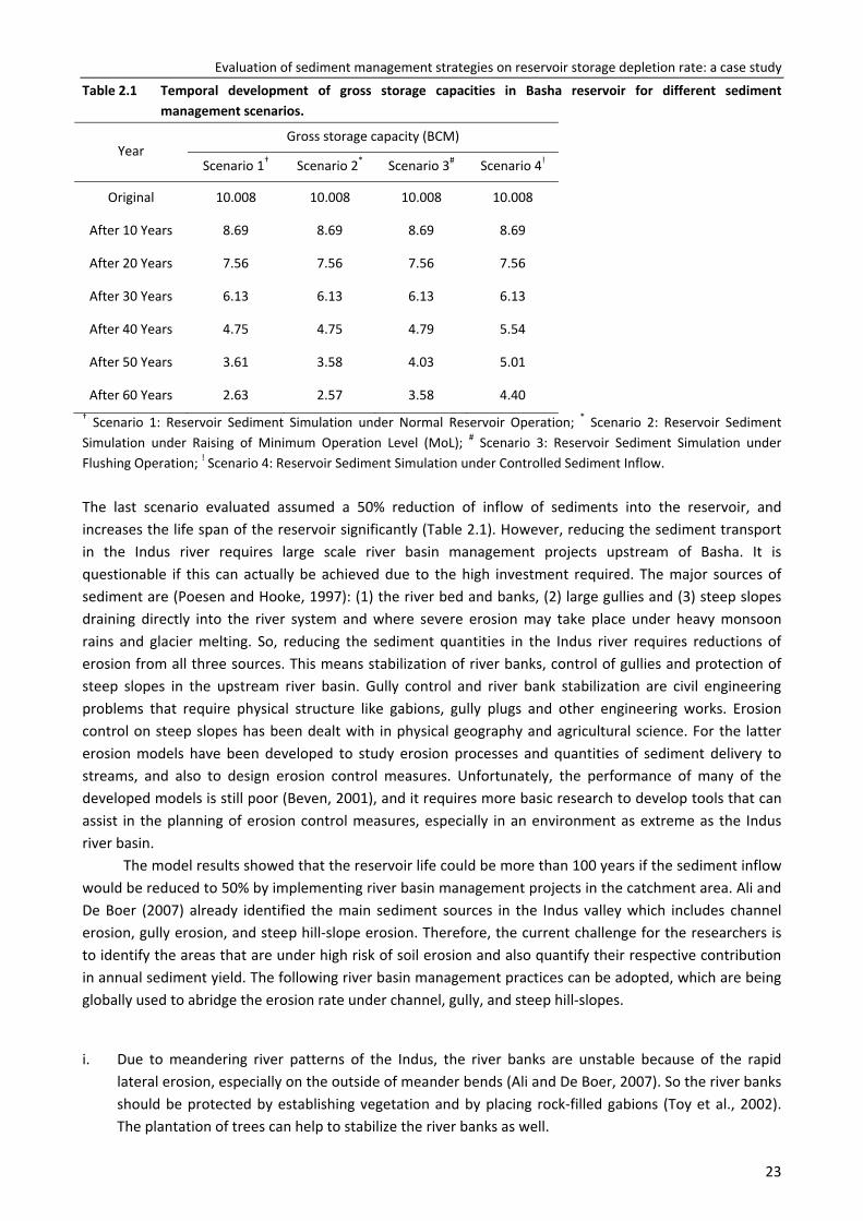
In order to mitigate the potential sedimentation dangers for the planned Basha reservoir, several sediment management strategies were evaluated and their impacts on reservoir storage depletion rate were studied. The operation of the Basha reservoir under different sediment management strategies exhibited substantial variation in storage capacity depletion rates (Table 2.1). Under normal reservoir operation, the RESSASS model calculated the annual storage loss of Basha reservoir is 1.23%, which is slightly higher than the global average annual depletion rate i.e. 1% (Mahmood, 1987). Also the already existing reservoir in the Indus river, i.e. Tarbela loses about 1% of storage annually (DBC, 2007; Ali et al., 2006). Considering the economic importance of hydropower reservoirs for Pakistan, there is a clear need for sediment management strategies to extend the lifetime of the planned Basha reservoir.
The selected sediment management strategies exhibited some advantages as well as disadvantages on the economic performance of the planned reservoir. The best reservoir operation strategy would be one which is environmental friendly and can significantly enhance the reservoir’s life. Table 2.1 presents the gross storage capacities for the different scenario’s of Basha reservoir. The gradual raising of MoL (scenario 2) has no effect on the lifetime of Basha reservoir, and results in exactly the same annual storage depletion as the normal operation (scenario 1). However, the raising of the MoL could reduce the movement of the sediment delta towards the dam, because the flow velocities are reduced. Due to low flow velocities, the coarse and fine sediments may deposit at the head of the reservoir (Figure 2.6).
Flushing of the reservoir will positively affect the lifetime of the planned reservoir (Table 2.1), with approximately 1.0 BCM more storage capacity after 60 years of operation. However, the flushing operation would be negatively affecting the life-span of the downstream Tarbela reservoir, because the flushed sediments will be transferred downstream and enter into the Tarbela reservoir. Also, flushing sediments from a large reservoir that is subject to high sedimentation rates is more difficult than for small reservoirs with low sedimentation rates (Liu et al., 2002). So both the flushing and raising of MoL would not be the preferred options, although these strategies may add 10 – 20 years to the life-span of Basha reservoir.
0
2
4
6
8
10
12
950 1000 1050 1100 1150 1200Water Level (m)
Rese
rvoi
r Sto
rage
Cap
acity
(BCM
)
Original
After 10 Years
After 20 Years
After 30 Years
After 40 YearsAfter 50 Years
After 60 Years
Evaluation of sediment management strategies on reservoir storage depletion rate: a case study
23
Table 2.1 Temporal development of gross storage capacities in Basha reservoir for different sediment management scenarios.
Year Gross storage capacity (BCM)
Scenario 1† Scenario 2* Scenario 3# Scenario 4!
Original 10.008 10.008 10.008 10.008
After 10 Years 8.69 8.69 8.69 8.69
After 20 Years 7.56 7.56 7.56 7.56
After 30 Years 6.13 6.13 6.13 6.13
After 40 Years 4.75 4.75 4.79 5.54
After 50 Years 3.61 3.58 4.03 5.01
After 60 Years 2.63 2.57 3.58 4.40 † Scenario 1: Reservoir Sediment Simulation under Normal Reservoir Operation; * Scenario 2: Reservoir Sediment Simulation under Raising of Minimum Operation Level (MoL); # Scenario 3: Reservoir Sediment Simulation under Flushing Operation; ! Scenario 4: Reservoir Sediment Simulation under Controlled Sediment Inflow. The last scenario evaluated assumed a 50% reduction of inflow of sediments into the reservoir, and increases the life span of the reservoir significantly (Table 2.1). However, reducing the sediment transport in the Indus river requires large scale river basin management projects upstream of Basha. It is questionable if this can actually be achieved due to the high investment required. The major sources of sediment are (Poesen and Hooke, 1997): (1) the river bed and banks, (2) large gullies and (3) steep slopes draining directly into the river system and where severe erosion may take place under heavy monsoon rains and glacier melting. So, reducing the sediment quantities in the Indus river requires reductions of erosion from all three sources. This means stabilization of river banks, control of gullies and protection of steep slopes in the upstream river basin. Gully control and river bank stabilization are civil engineering problems that require physical structure like gabions, gully plugs and other engineering works. Erosion control on steep slopes has been dealt with in physical geography and agricultural science. For the latter erosion models have been developed to study erosion processes and quantities of sediment delivery to streams, and also to design erosion control measures. Unfortunately, the performance of many of the developed models is still poor (Beven, 2001), and it requires more basic research to develop tools that can assist in the planning of erosion control measures, especially in an environment as extreme as the Indus river basin.
The model results showed that the reservoir life could be more than 100 years if the sediment inflow would be reduced to 50% by implementing river basin management projects in the catchment area. Ali and De Boer (2007) already identified the main sediment sources in the Indus valley which includes channel erosion, gully erosion, and steep hill-slope erosion. Therefore, the current challenge for the researchers is to identify the areas that are under high risk of soil erosion and also quantify their respective contribution in annual sediment yield. The following river basin management practices can be adopted, which are being globally used to abridge the erosion rate under channel, gully, and steep hill-slopes.
i. Due to meandering river patterns of the Indus, the river banks are unstable because of the rapid lateral erosion, especially on the outside of meander bends (Ali and De Boer, 2007). So the river banks should be protected by establishing vegetation and by placing rock-filled gabions (Toy et al., 2002). The plantation of trees can help to stabilize the river banks as well.

Chapter 2
24
ii. Under gully erosion, the detachment and transport of sediment could be due to high flow velocities and steep slopes, which can be controlled by constructing check dams to reduce the flow velocities (Zhou et al., 2004). The check-dams would be effective in both the glacier melt and rain induced areas.
iii. The soil losses on hill-slopes are mainly due to interrill and rill erosion. Therefore, the detachment and transport capacity on hill slopes can be reduced by introducing strips of dense vegetation, terraces, flow diversions and armored waterways for runoff disposal (Toy et al., 2002). The vegetation must be appropriate for the local climate and soil conditions.
The river basin management projects would not only have positive impacts on the life of Basha reservoir, but may also extend the life of projects that are being planned to construct upstream and downstream of Basha. The proposed watershed management practices may enhance the agriculture production in the area, which would have direct impact on the life of local people.
Chapter 3
Availability and performance of sediment detachment and transport functions for overland flow conditions
Ali M. and G. Sterk Progress in Physical Geography (in review)

27
Availability and performance of sediment detachment and transport functions for overland flow conditions
Abstract
Soil erosion is a global environment problem. In order to quantify water erosion rates at the field, hillslope or catchment scale, several spatially distributed soil erosion models have been developed. The accuracy of those erosion models depends largely on the used sediment detachment and sediment transport functions. Many of such functions were developed from empirical research, usually under laboratory conditions. The aim of this paper was to review the physical basis of the available sediment detachment and sediment transport functions, and to determine their application boundaries. Well-known and widely used sediment detachment and sediment transport functions are discussed on the basis of composite force predictors i.e. shear stress, stream power, unit stream power and effective stream power. The suitability of these functions for overland flow conditions was elucidated on the basis of information available in the literature. It was found that only few sediment detachment functions are available, and those have been poorly tested for overland flow conditions. It is concluded that the suitability of existing sediment detachment functions should be checked for a wider range of laboratory and field conditions. Most erosion models ignore direct calculation of sediment detachment, but use the sediment transport capacity deficit approach to estimate detachment rate. There are much more sediment transport functions available, and they were also better tested for overland flow conditions. However, the testing of the available sediment transport functions for overland flow conditions did not result in one single function that appeared to perform best under a range of experimental conditions. The Govers (1990) and Govers (1992a) unit stream power based functions seem to be the most promising functions for water erosion modelling. It is still recommended to evaluate the performance of existing sediment transport functions with more detailed field and laboratory datasets.
3.1 Introduction
Soil erosion is a common global problem that adversely affects the productivity of agriculture (Lal and Stewart, 1990; Pimentel et al., 1995; Yang et al., 2003). Severe erosion may occur when unprotected soil is exposed to rain or wind energy (Barrow, 1991). According to Barrow (1991), globally 75 billion tons of soil are eroded from agricultural lands and around 20 million hectares of land are lost due to erosion each year. Soil erosion rates are high in Asia, Africa and South America, averaging 30–40 t ha-1 yr-1 (Barrow, 1991). Estimates for Asia are higher than the averages given by Barrow (1991), and are in the order of 138 t ha-1 yr-1 (Sfeir-Younis, 1986). Erosion causes land degradation and reduces crop production potential, while the eroded sediment contaminates surface waters and reduces the storage capacity of reservoirs that directly affects irrigated agriculture and hydro–electricity generation. Soil erosion is also one of the main causes of global warming because it emits CO2 and CH4 gases from soil to the atmosphere (Lal, 2004).
To assess water erosion problems in catchments, scientists have developed several spatially distributed soil erosion models with various degree of sophistication. Examples are CREAMS (Knisel, 1980), KYERMO (Hirschi and Barfield, 1988a,b), PRORILL (Lewis et al., 1994a,b), KINEROS2 (Smith et al., 1995), LISEM (De Roo et al., 1996), RUSLE (Renard et al., 1997), EUROSEM (Morgan et al., 1998a,b), EGEM (Woodward, 1999), GLEAMS (Knisel and Davis, 2000), and WEPP (Flanagan et al., 2001). Some of those models are fully empirical (e.g. RUSLE) while others are physically-based (e.g. KINEROS2), approaching the erosion problem from physical laws (Beven, 2001). Those empirical and physically-based models have been
Chapter 3
28
applied in catchment-scale erosion studies with varying degrees of success (e.g. Kim et al., 2007; Larsen and MacDonald, 2007).
Sediment detachment and transport are important sub-processes in water erosion. These two components of soil erosion are critically interlinked with each other (Foster and Meyer, 1972). Accurate prediction of sediment detachment and transport rates is of much importance in the development of a water erosion model. Correct calculations of the amounts of sediment detachment and transport play a vital role in the accuracy of the outcomes of each spatially distributed soil erosion model. For both sub-processes in water erosion there is a variety of predictive functions available.
The detachment functions used in most models are of empirical nature and were derived from experimental data (e.g. Foster, 1982; Elliot and Laflen, 1993). The empiricism may cause problems when those detachment functions are used outside the experimental domain for which they were derived. Most of the existing sediment transport functions were originally derived for channel flow. These functions are commonly used in several physically based soil erosion models to estimate sediment transport in shallow overland flows (Smith et al., 1995; Flanagan et al., 2001). But, the applicability of stream flow functions has become questionable under overland flow, because the water layer depths and discharges are usually much smaller in overland flow. Moreover, hillslope surfaces are usually rougher than streams. This is due to obstacles at the surface, such as stones, plant stems, leaves, etc. Such higher values of roughness substantially reduce the transport capacity of the flow (Govers and Rauws, 1986; Abrahams and Parsons, 1994; Abrahams et al., 2000). Also raindrops can disturb the thin overland flow layers, which is not the case for channel flow, where the water depth is sufficient. It is therefore questionable if those functions give reliable results for water erosion predictions under overland flow conditions.
Given the importance of sediment detachment and transport functions for accurate water erosion modelling, it is important to know what the physical basis of the main functions is and how well these functions perform under different experimental conditions. The main aim of this paper was to review and summarize the available information about sediment detachment and transport functions which are often used in spatially distributed soil erosion models. The review encompasses (i) processes engaged in soil erosion (ii) the availability and performance of soil detachment functions for overland flow conditions, and (iii) the availability and performance of sediment transport functions for overland flow conditions.
3.2 Processes of Sediment Detachment and Transport by Overland Flow
The soil erosion process by water is usually described in two steps i.e. detachment and transport (Ellison, 1947). Soil detachment is the dislodgement of soil particles from the soil mass, while transport is the movement of soil particles from one location to another (Foster and Meyer, 1972). The dislodgement of soil particles is mainly caused by the forces applied by raindrops and overland flow. Detachment of soil particles by raindrops depends on several variables such as rain drop size, fall velocity, rainfall intensity, soil erodibility, etc. (Owoputi and Stolte, 1995). The impact of raindrops on sediment transport in the absence of overland flow, i.e. splash erosion has been comprehensively studied (Poesen and Savat, 1981; Savat, 1981; Moss and Green, 1983), and is not considered in this paper. Here we deal with detachment and transport of sediment by layers of overland flow only.
Detachment by overland flow is caused by the forces of the layer of flowing water affecting the soil surface. Theoretically, a given layer of overland flow on a certain slope can detach a maximum amount of sediment, indicated by the detachment capacity (Dc). The actual rate of detachment (Dr) will normally be lower than the detachment capacity, because the maximum detachment can only occur with clean water that contains no sediments (Foster and Meyer, 1972).
Sediment transport is also an important component of the soil erosion process. Under overland flow conditions, sediment can be transported in the form of bedload and suspended load (Allen, 1994). The
Availability and performance of sediment detachment and transport functions
29
sediment transport rate (Tr) mainly depends upon the transport capacity (Tc) of overland flow. The sediment transport capacity of overland flow is defined as the maximum amount of sediment that can be transported at a particular discharge on a certain slope (Merten et al., 2001). Several studies have shown that the transport capacity of overland flow is dependent on bed slope, discharge, flow velocity, flow depth and sediment particle size (Nearing et al., 1991; Zhang et al., 2003).
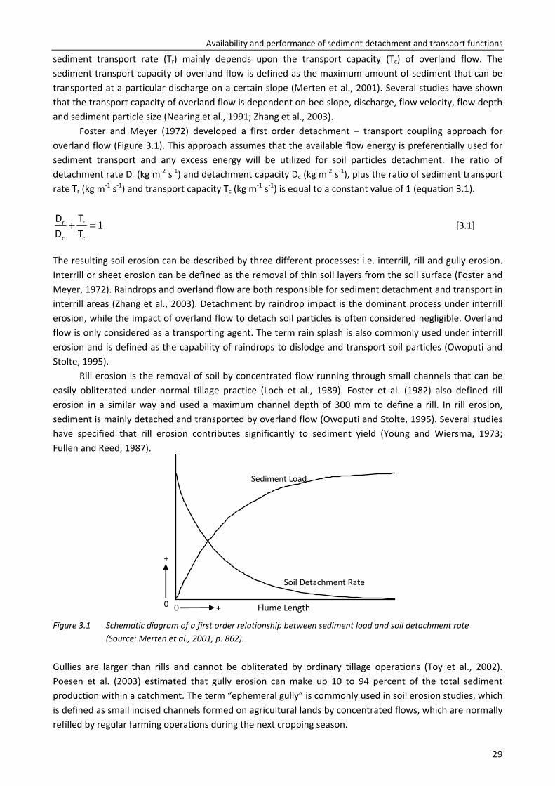
Foster and Meyer (1972) developed a first order detachment – transport coupling approach for overland flow (Figure 3.1). This approach assumes that the available flow energy is preferentially used for sediment transport and any excess energy will be utilized for soil particles detachment. The ratio of detachment rate Dr (kg m-2 s-1) and detachment capacity Dc (kg m-2 s-1), plus the ratio of sediment transport rate Tr (kg m-1 s-1) and transport capacity Tc (kg m-1 s-1) is equal to a constant value of 1 (equation 3.1).
1TT
DD
c
r
c
r =+ [3.1]
The resulting soil erosion can be described by three different processes: i.e. interrill, rill and gully erosion. Interrill or sheet erosion can be defined as the removal of thin soil layers from the soil surface (Foster and Meyer, 1972). Raindrops and overland flow are both responsible for sediment detachment and transport in interrill areas (Zhang et al., 2003). Detachment by raindrop impact is the dominant process under interrill erosion, while the impact of overland flow to detach soil particles is often considered negligible. Overland flow is only considered as a transporting agent. The term rain splash is also commonly used under interrill erosion and is defined as the capability of raindrops to dislodge and transport soil particles (Owoputi and Stolte, 1995).
Rill erosion is the removal of soil by concentrated flow running through small channels that can be easily obliterated under normal tillage practice (Loch et al., 1989). Foster et al. (1982) also defined rill erosion in a similar way and used a maximum channel depth of 300 mm to define a rill. In rill erosion, sediment is mainly detached and transported by overland flow (Owoputi and Stolte, 1995). Several studies have specified that rill erosion contributes significantly to sediment yield (Young and Wiersma, 1973; Fullen and Reed, 1987).
Figure 3.1 Schematic diagram of a first order relationship between sediment load and soil detachment rate (Source: Merten et al., 2001, p. 862). Gullies are larger than rills and cannot be obliterated by ordinary tillage operations (Toy et al., 2002). Poesen et al. (2003) estimated that gully erosion can make up 10 to 94 percent of the total sediment production within a catchment. The term “ephemeral gully” is commonly used in soil erosion studies, which is defined as small incised channels formed on agricultural lands by concentrated flows, which are normally refilled by regular farming operations during the next cropping season.
Flume Length00
+
+
Sediment Load
Soil Detachment Rate
Chapter 3
30
In this paper only those sediment detachment and transport functions will be reviewed which are used for interill and rill erosion conditions. Hence, only thin layers of overland flow are considered, which excludes gully formation as the layers of overland flow become much thicker then.
3.3 Detachment and Transport Predictors
Most detachment and transport functions were derived from laboratory (flume) experimental data, in which the transport of non-cohesive homogeneous sediment was studied under controlled hydraulic conditions. The rate of sediment detachment and transport under overland flow depends on many hydraulic and sediment parameters like flow discharge, bed slope gradient, flow depth, flow velocity, particle size, bed roughness elements, and rainfall impact. Several researchers studied the impact of slope gradient, flow discharge, flow velocity, and flow depth on sediment transport capacity (Govers, 1992a; Abrahams et al., 1996; Liu et al., 2000). These hydraulic variables are well parameterized in existing detachment and sediment transport capacity functions to predict detachment and transport capacity of overland flow as a function of a driving force. The most widely used composite force predictors are shear stress, stream power, unit stream power and effective stream power.
3.3.1 Shear Stress Shear stress (τ) is the force per unit area applied by flowing water on the soil surface. It is defined according to equation 3.2 (Beven, 2001).
gRSρ=τ (N m-2) [3.2]
Where ρ (kg m-3) is the water density, g (N kg-1) is the acceleration due to gravity, R is the hydraulic radius which is assumed equal to flow depth (h in m) under overland flow, and S (m m-1) is the slope gradient. 3.3.2 Stream Power Bagnold (1966) introduced the concept of stream power (ω) by assuming that the sediment transport rate should be related to the time rate of potential energy expenditure per unit bed area. His study clearly demonstrated that the ability of a stream to transport sediment depends on its available power, and not on its available energy (Yang, 1973). Stream power is defined as the product of shear stress and the average flow velocity (equation 3.3).
τ=ω u (J m-2 s-1) [3.3]
Where u (m s-1) is the mean flow velocity.
3.3.3 Unit Stream Power Yang (1972) assumed that the sediment transport rate should be related to the time rate of potential energy dissipation per unit weight of water. He defined unit steam power (ωu) as the product of average flow velocity and slope gradient:
Suu =ω (m s-1) [3.4]
The basic difference between the stream power and unit stream power is that the stream power deals with the power per unit bed area and unit stream power deals with the power per unit weight of water.
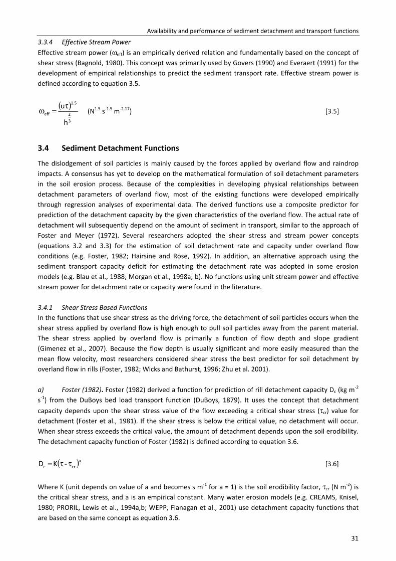
Availability and performance of sediment detachment and transport functions
31
3.3.4 Effective Stream Power Effective stream power (ωeff) is an empirically derived relation and fundamentally based on the concept of shear stress (Bagnold, 1980). This concept was primarily used by Govers (1990) and Everaert (1991) for the development of empirical relationships to predict the sediment transport rate. Effective stream power is defined according to equation 3.5.
( )32
5.1
eff
h
uτ=ω (N1.5 s-1.5 m-2.17) [3.5]
3.4 Sediment Detachment Functions
The dislodgement of soil particles is mainly caused by the forces applied by overland flow and raindrop impacts. A consensus has yet to develop on the mathematical formulation of soil detachment parameters in the soil erosion process. Because of the complexities in developing physical relationships between detachment parameters of overland flow, most of the existing functions were developed empirically through regression analyses of experimental data. The derived functions use a composite predictor for prediction of the detachment capacity by the given characteristics of the overland flow. The actual rate of detachment will subsequently depend on the amount of sediment in transport, similar to the approach of Foster and Meyer (1972). Several researchers adopted the shear stress and stream power concepts (equations 3.2 and 3.3) for the estimation of soil detachment rate and capacity under overland flow conditions (e.g. Foster, 1982; Hairsine and Rose, 1992). In addition, an alternative approach using the sediment transport capacity deficit for estimating the detachment rate was adopted in some erosion models (e.g. Blau et al., 1988; Morgan et al., 1998a; b). No functions using unit stream power and effective stream power for detachment rate or capacity were found in the literature.
3.4.1 Shear Stress Based Functions In the functions that use shear stress as the driving force, the detachment of soil particles occurs when the shear stress applied by overland flow is high enough to pull soil particles away from the parent material. The shear stress applied by overland flow is primarily a function of flow depth and slope gradient (Gimenez et al., 2007). Because the flow depth is usually significant and more easily measured than the mean flow velocity, most researchers considered shear stress the best predictor for soil detachment by overland flow in rills (Foster, 1982; Wicks and Bathurst, 1996; Zhu et al. 2001).
a) Foster (1982). Foster (1982) derived a function for prediction of rill detachment capacity Dc (kg m-2 s-1) from the DuBoys bed load transport function (DuBoys, 1879). It uses the concept that detachment capacity depends upon the shear stress value of the flow exceeding a critical shear stress (τcr) value for detachment (Foster et al., 1981). If the shear stress is below the critical value, no detachment will occur. When shear stress exceeds the critical value, the amount of detachment depends upon the soil erodibility. The detachment capacity function of Foster (1982) is defined according to equation 3.6.
( )acrc KD ττ= - [3.6]
Where K (unit depends on value of a and becomes s m-1 for a = 1) is the soil erodibility factor, τcr (N m-2) is the critical shear stress, and a is an empirical constant. Many water erosion models (e.g. CREAMS, Knisel, 1980; PRORIL, Lewis et al., 1994a,b; WEPP, Flanagan et al., 2001) use detachment capacity functions that are based on the same concept as equation 3.6.
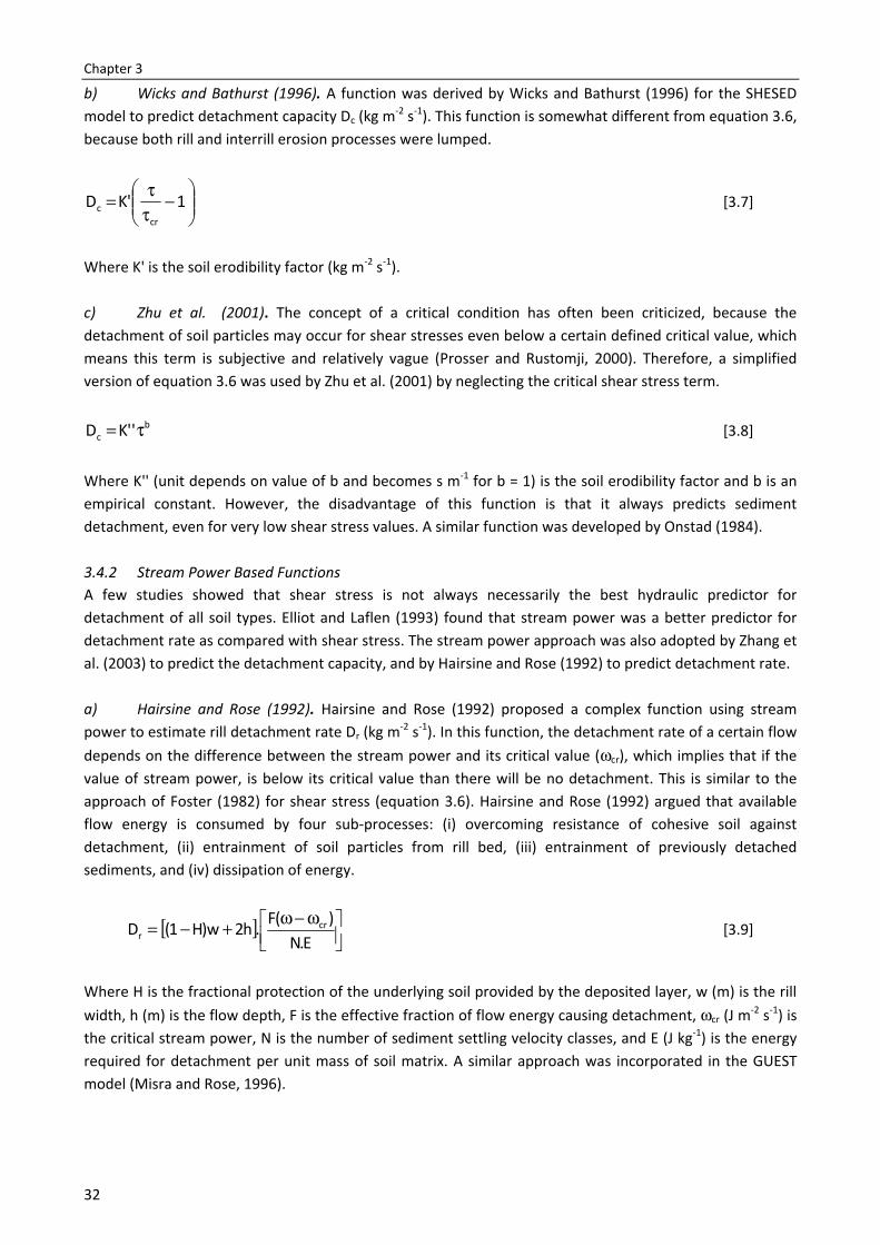
Chapter 3
32
b) Wicks and Bathurst (1996). A function was derived by Wicks and Bathurst (1996) for the SHESED model to predict detachment capacity Dc (kg m-2 s-1). This function is somewhat different from equation 3.6, because both rill and interrill erosion processes were lumped.
−
ττ= 1'KDcr
c [3.7]
Where K' is the soil erodibility factor (kg m-2 s-1).
c) Zhu et al. (2001). The concept of a critical condition has often been criticized, because the detachment of soil particles may occur for shear stresses even below a certain defined critical value, which means this term is subjective and relatively vague (Prosser and Rustomji, 2000). Therefore, a simplified version of equation 3.6 was used by Zhu et al. (2001) by neglecting the critical shear stress term.
b
c ''KD τ= [3.8]
Where K'' (unit depends on value of b and becomes s m-1 for b = 1) is the soil erodibility factor and b is an empirical constant. However, the disadvantage of this function is that it always predicts sediment detachment, even for very low shear stress values. A similar function was developed by Onstad (1984).
3.4.2 Stream Power Based Functions A few studies showed that shear stress is not always necessarily the best hydraulic predictor for detachment of all soil types. Elliot and Laflen (1993) found that stream power was a better predictor for detachment rate as compared with shear stress. The stream power approach was also adopted by Zhang et al. (2003) to predict the detachment capacity, and by Hairsine and Rose (1992) to predict detachment rate.
a) Hairsine and Rose (1992). Hairsine and Rose (1992) proposed a complex function using stream power to estimate rill detachment rate Dr (kg m-2 s-1). In this function, the detachment rate of a certain flow depends on the difference between the stream power and its critical value (ωcr), which implies that if the value of stream power, is below its critical value than there will be no detachment. This is similar to the approach of Foster (1982) for shear stress (equation 3.6). Hairsine and Rose (1992) argued that available flow energy is consumed by four sub-processes: (i) overcoming resistance of cohesive soil against detachment, (ii) entrainment of soil particles from rill bed, (iii) entrainment of previously detached sediments, and (iv) dissipation of energy.
[ ]
ω−ω+−=
E.N)(F.h2w)H1(D cr
r [3.9]
Where H is the fractional protection of the underlying soil provided by the deposited layer, w (m) is the rill width, h (m) is the flow depth, F is the effective fraction of flow energy causing detachment, ωcr (J m-2 s-1) is the critical stream power, N is the number of sediment settling velocity classes, and E (J kg-1) is the energy required for detachment per unit mass of soil matrix. A similar approach was incorporated in the GUEST model (Misra and Rose, 1996).
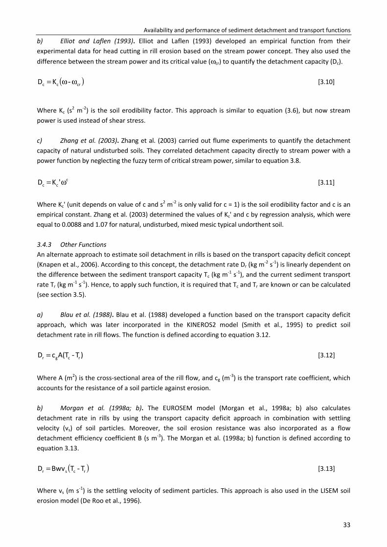
Availability and performance of sediment detachment and transport functions
33
b) Elliot and Laflen (1993). Elliot and Laflen (1993) developed an empirical function from their experimental data for head cutting in rill erosion based on the stream power concept. They also used the difference between the stream power and its critical value (ωcr) to quantify the detachment capacity (Dc).
( )crcc KD ωω= - [3.10]
Where Kc (s2 m-2) is the soil erodibility factor. This approach is similar to equation (3.6), but now stream power is used instead of shear stress.
c) Zhang et al. (2003). Zhang et al. (2003) carried out flume experiments to quantify the detachment capacity of natural undisturbed soils. They correlated detachment capacity directly to stream power with a power function by neglecting the fuzzy term of critical stream power, similar to equation 3.8.
c
cc 'KD ω= [3.11]
Where Kc' (unit depends on value of c and s2 m-2 is only valid for c = 1) is the soil erodibility factor and c is an empirical constant. Zhang et al. (2003) determined the values of Kc' and c by regression analysis, which were equal to 0.0088 and 1.07 for natural, undisturbed, mixed mesic typical undorthent soil.
3.4.3 Other Functions An alternate approach to estimate soil detachment in rills is based on the transport capacity deficit concept (Knapen et al., 2006). According to this concept, the detachment rate Dr (kg m-2 s-1) is linearly dependent on the difference between the sediment transport capacity Tc (kg m-1 s-1), and the current sediment transport rate Tr (kg m-1 s-1). Hence, to apply such function, it is required that Tc and Tr are known or can be calculated (see section 3.5).
a) Blau et al. (1988). Blau et al. (1988) developed a function based on the transport capacity deficit approach, which was later incorporated in the KINEROS2 model (Smith et al., 1995) to predict soil detachment rate in rill flows. The function is defined according to equation 3.12.
)TT(AcD rcgr -= [3.12]
Where A (m2) is the cross-sectional area of the rill flow, and cg (m-3) is the transport rate coefficient, which accounts for the resistance of a soil particle against erosion.
b) Morgan et al. (1998a; b). The EUROSEM model (Morgan et al., 1998a; b) also calculates detachment rate in rills by using the transport capacity deficit approach in combination with settling velocity (vs) of soil particles. Moreover, the soil erosion resistance was also incorporated as a flow detachment efficiency coefficient B (s m-3). The Morgan et al. (1998a; b) function is defined according to equation 3.13.
( )rcsr TTBwvD -= [3.13]
Where vs (m s-1) is the settling velocity of sediment particles. This approach is also used in the LISEM soil erosion model (De Roo et al., 1996).
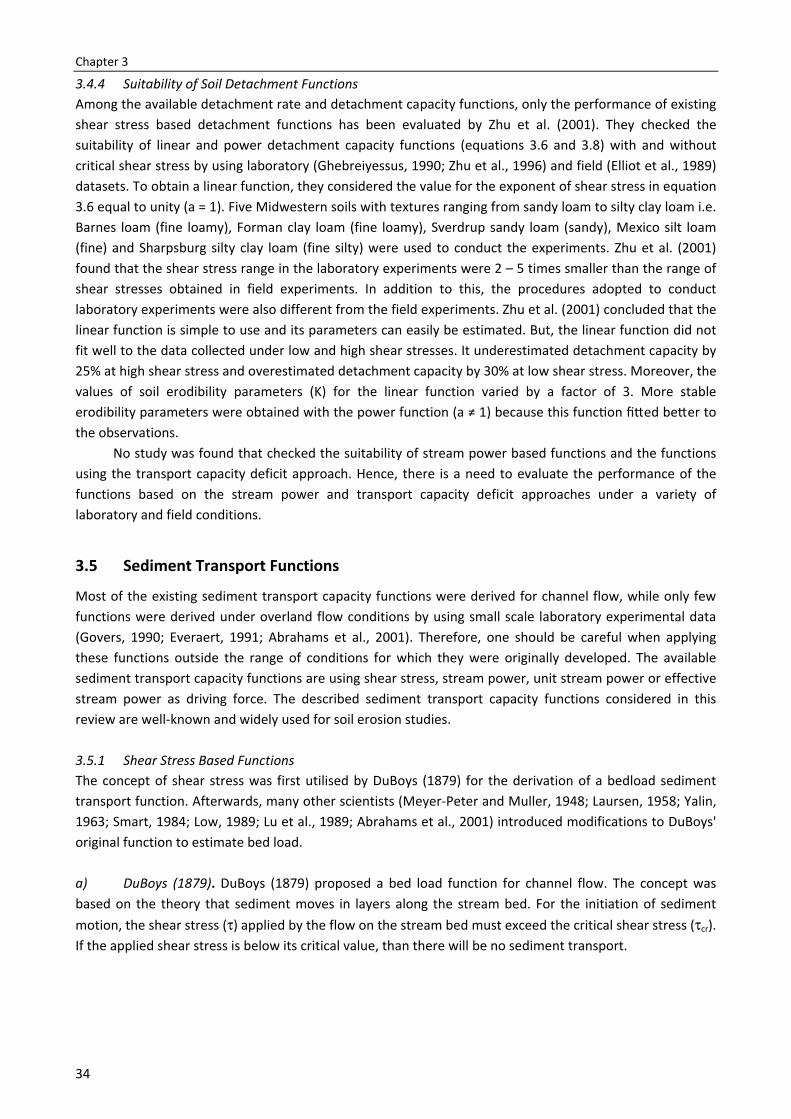
Chapter 3
34
3.4.4 Suitability of Soil Detachment Functions Among the available detachment rate and detachment capacity functions, only the performance of existing shear stress based detachment functions has been evaluated by Zhu et al. (2001). They checked the suitability of linear and power detachment capacity functions (equations 3.6 and 3.8) with and without critical shear stress by using laboratory (Ghebreiyessus, 1990; Zhu et al., 1996) and field (Elliot et al., 1989) datasets. To obtain a linear function, they considered the value for the exponent of shear stress in equation 3.6 equal to unity (a = 1). Five Midwestern soils with textures ranging from sandy loam to silty clay loam i.e. Barnes loam (fine loamy), Forman clay loam (fine loamy), Sverdrup sandy loam (sandy), Mexico silt loam (fine) and Sharpsburg silty clay loam (fine silty) were used to conduct the experiments. Zhu et al. (2001) found that the shear stress range in the laboratory experiments were 2 – 5 times smaller than the range of shear stresses obtained in field experiments. In addition to this, the procedures adopted to conduct laboratory experiments were also different from the field experiments. Zhu et al. (2001) concluded that the linear function is simple to use and its parameters can easily be estimated. But, the linear function did not fit well to the data collected under low and high shear stresses. It underestimated detachment capacity by 25% at high shear stress and overestimated detachment capacity by 30% at low shear stress. Moreover, the values of soil erodibility parameters (K) for the linear function varied by a factor of 3. More stable erodibility parameters were obtained with the power function (a ≠ 1) because this func on fi ed be er to the observations.
No study was found that checked the suitability of stream power based functions and the functions using the transport capacity deficit approach. Hence, there is a need to evaluate the performance of the functions based on the stream power and transport capacity deficit approaches under a variety of laboratory and field conditions.
3.5 Sediment Transport Functions
Most of the existing sediment transport capacity functions were derived for channel flow, while only few functions were derived under overland flow conditions by using small scale laboratory experimental data (Govers, 1990; Everaert, 1991; Abrahams et al., 2001). Therefore, one should be careful when applying these functions outside the range of conditions for which they were originally developed. The available sediment transport capacity functions are using shear stress, stream power, unit stream power or effective stream power as driving force. The described sediment transport capacity functions considered in this review are well-known and widely used for soil erosion studies.
3.5.1 Shear Stress Based Functions The concept of shear stress was first utilised by DuBoys (1879) for the derivation of a bedload sediment transport function. Afterwards, many other scientists (Meyer-Peter and Muller, 1948; Laursen, 1958; Yalin, 1963; Smart, 1984; Low, 1989; Lu et al., 1989; Abrahams et al., 2001) introduced modifications to DuBoys' original function to estimate bed load.
a) DuBoys (1879). DuBoys (1879) proposed a bed load function for channel flow. The concept was based on the theory that sediment moves in layers along the stream bed. For the initiation of sediment motion, the shear stress (τ) applied by the flow on the stream bed must exceed the critical shear stress (τcr). If the applied shear stress is below its critical value, than there will be no sediment transport.
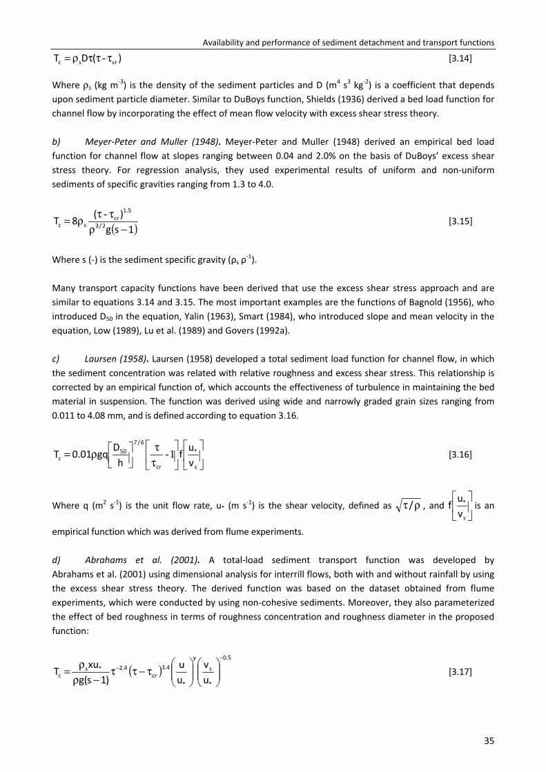
Availability and performance of sediment detachment and transport functions
35
)(DT crsc τττρ= - [3.14]
Where ρs (kg m-3) is the density of the sediment particles and D (m4 s3 kg-2) is a coefficient that depends upon sediment particle diameter. Similar to DuBoys function, Shields (1936) derived a bed load function for channel flow by incorporating the effect of mean flow velocity with excess shear stress theory.
b) Meyer-Peter and Muller (1948). Meyer-Peter and Muller (1948) derived an empirical bed load function for channel flow at slopes ranging between 0.04 and 2.0% on the basis of DuBoys’ excess shear stress theory. For regression analysis, they used experimental results of uniform and non-uniform sediments of specific gravities ranging from 1.3 to 4.0.
( )1sg)(8T 2/3
5.1cr
sc −ρττρ= -
[3.15]
Where s (-) is the sediment specific gravity (ρs ρ-1).
Many transport capacity functions have been derived that use the excess shear stress approach and are similar to equations 3.14 and 3.15. The most important examples are the functions of Bagnold (1956), who introduced D50 in the equation, Yalin (1963), Smart (1984), who introduced slope and mean velocity in the equation, Low (1989), Lu et al. (1989) and Govers (1992a).
c) Laursen (1958). Laursen (1958) developed a total sediment load function for channel flow, in which the sediment concentration was related with relative roughness and excess shear stress. This relationship is corrected by an empirical function of, which accounts the effectiveness of turbulence in maintaining the bed material in suspension. The function was derived using wide and narrowly graded grain sizes ranging from 0.011 to 4.08 mm, and is defined according to equation 3.16.
ττ
ρ=
s
*
cr
6/750
c vuf
hDgq01.0T 1- [3.16]
Where q (m2 s-1) is the unit flow rate, u* (m s-1) is the shear velocity, defined as ρτ/ , and
s
*
vuf is an
empirical function which was derived from flume experiments.
d) Abrahams et al. (2001). A total-load sediment transport function was developed by Abrahams et al. (2001) using dimensional analysis for interrill flows, both with and without rainfall by using the excess shear stress theory. The derived function was based on the dataset obtained from flume experiments, which were conducted by using non-cohesive sediments. Moreover, they also parameterized the effect of bed roughness in terms of roughness concentration and roughness diameter in the proposed function:
( )5.0
*
s
y
*
4.3cr
4.2*sc u
vuu
)1s(gxuT
−−
τ−ττ
−ρρ= [3.17]
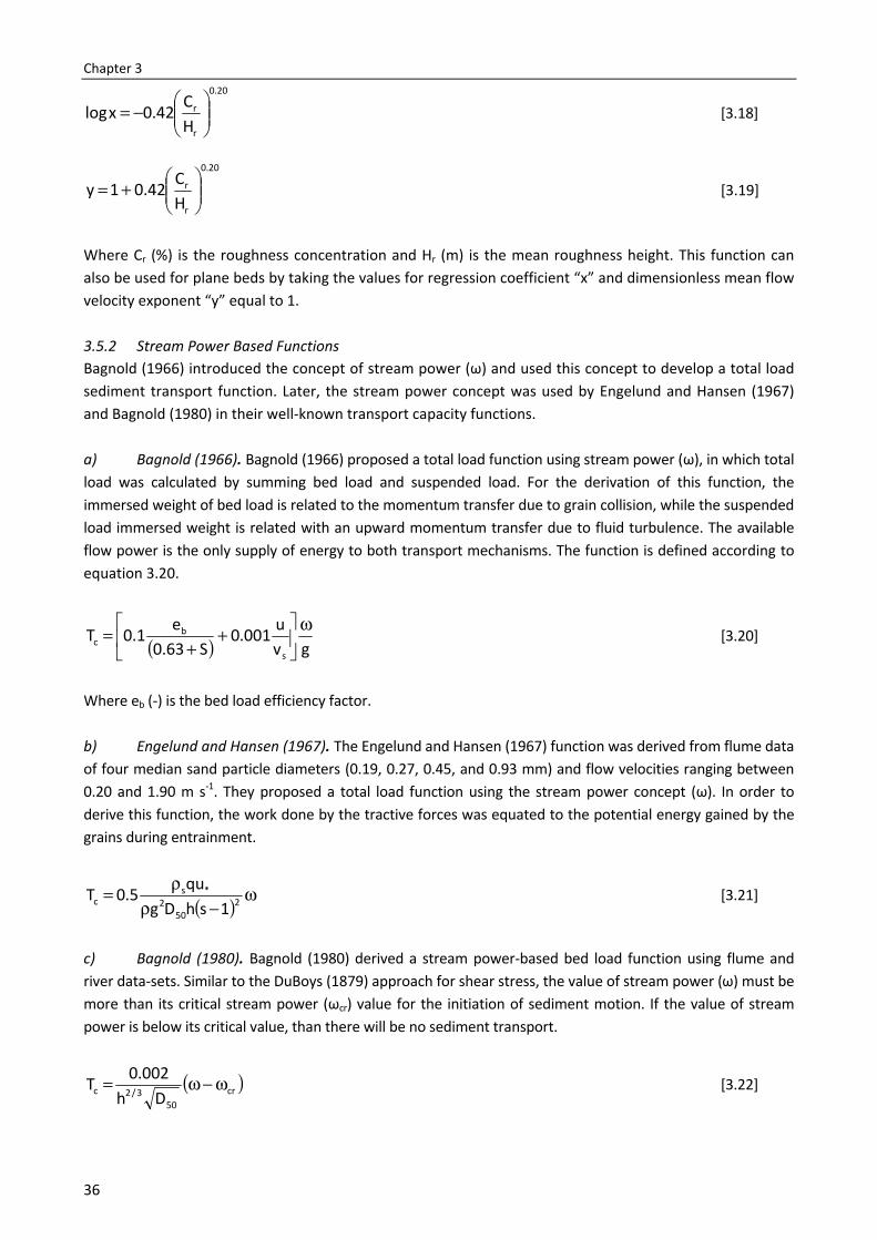
Chapter 3
36
20.0
r
r
HC42.0xlog
−= [3.18]
20.0
r
r
HC42.01y
+= [3.19]
Where Cr (%) is the roughness concentration and Hr (m) is the mean roughness height. This function can also be used for plane beds by taking the values for regression coefficient “x” and dimensionless mean flow velocity exponent “y” equal to 1.
3.5.2 Stream Power Based Functions Bagnold (1966) introduced the concept of stream power (ω) and used this concept to develop a total load sediment transport function. Later, the stream power concept was used by Engelund and Hansen (1967) and Bagnold (1980) in their well-known transport capacity functions.
a) Bagnold (1966). Bagnold (1966) proposed a total load function using stream power (ω), in which total load was calculated by summing bed load and suspended load. For the derivation of this function, the immersed weight of bed load is related to the momentum transfer due to grain collision, while the suspended load immersed weight is related with an upward momentum transfer due to fluid turbulence. The available flow power is the only supply of energy to both transport mechanisms. The function is defined according to equation 3.20.
( ) gvu001.0
S63.0e1.0T
s
bc
ω
+
+= [3.20]
Where eb (-) is the bed load efficiency factor.
b) Engelund and Hansen (1967). The Engelund and Hansen (1967) function was derived from flume data of four median sand particle diameters (0.19, 0.27, 0.45, and 0.93 mm) and flow velocities ranging between 0.20 and 1.90 m s-1. They proposed a total load function using the stream power concept (ω). In order to derive this function, the work done by the tractive forces was equated to the potential energy gained by the grains during entrainment.
( ) ω−ρ
ρ= 250
2*s
c 1shDgqu5.0T [3.21]
c) Bagnold (1980). Bagnold (1980) derived a stream power-based bed load function using flume and river data-sets. Similar to the DuBoys (1879) approach for shear stress, the value of stream power (ω) must be more than its critical stream power (ωcr) value for the initiation of sediment motion. If the value of stream power is below its critical value, than there will be no sediment transport.
( )cr50
3/2c Dh002.0T ω−ω= [3.22]
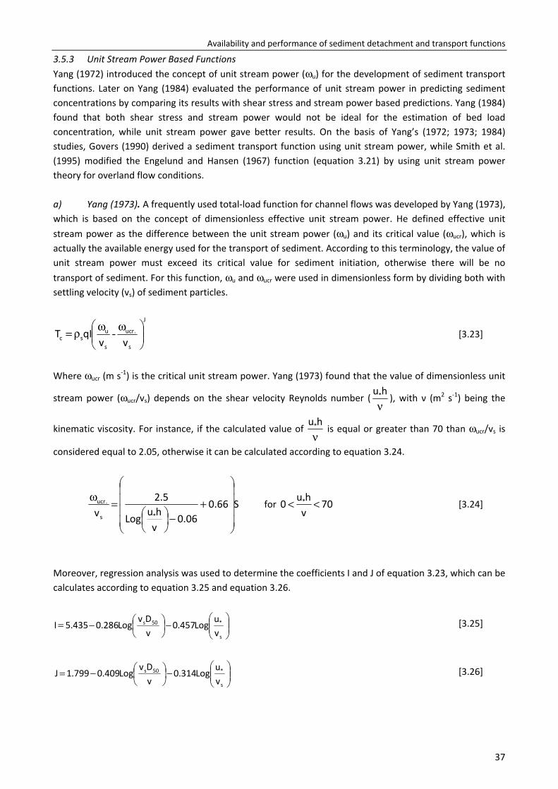
Availability and performance of sediment detachment and transport functions
37
3.5.3 Unit Stream Power Based Functions Yang (1972) introduced the concept of unit stream power (ωu) for the development of sediment transport functions. Later on Yang (1984) evaluated the performance of unit stream power in predicting sediment concentrations by comparing its results with shear stress and stream power based predictions. Yang (1984) found that both shear stress and stream power would not be ideal for the estimation of bed load concentration, while unit stream power gave better results. On the basis of Yang’s (1972; 1973; 1984) studies, Govers (1990) derived a sediment transport function using unit stream power, while Smith et al. (1995) modified the Engelund and Hansen (1967) function (equation 3.21) by using unit stream power theory for overland flow conditions.
a) Yang (1973). A frequently used total-load function for channel flows was developed by Yang (1973), which is based on the concept of dimensionless effective unit stream power. He defined effective unit stream power as the difference between the unit stream power (ωu) and its critical value (ωucr), which is actually the available energy used for the transport of sediment. According to this terminology, the value of unit stream power must exceed its critical value for sediment initiation, otherwise there will be no transport of sediment. For this function, ωu and ωucr were used in dimensionless form by dividing both with settling velocity (vs) of sediment particles.
J
s
.ucr
s
usc vvqIT
ωωρ= - [3.23]
Where ωucr (m s-1) is the critical unit stream power. Yang (1973) found that the value of dimensionless unit
stream power (ωucr/vs) depends on the shear velocity Reynolds number (νhu* ), with ν (m2 s-1) being the
kinematic viscosity. For instance, if the calculated value of νhu* is equal or greater than 70 than ωucr/vs is
considered equal to 2.05, otherwise it can be calculated according to equation 3.24.
S66.006.0
vhuLog
5.2v *s
.ucr
+−
=ω for 70
vhu0 * << [3.24]
Moreover, regression analysis was used to determine the coefficients I and J of equation 3.23, which can be calculates according to equation 3.25 and equation 3.26.
−
−=
s
*50s
vuLog457.0
vDv
Log286.0435.5I [3.25]
−
−=
s
*50s
vuLog314.0
vDv
Log409.0799.1J [3.26]
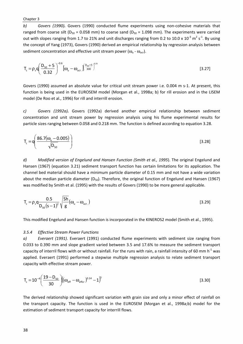
Chapter 3
38
b) Govers (1990). Govers (1990) conducted flume experiments using non-cohesive materials that ranged from coarse silt (D50 = 0.058 mm) to coarse sand (D50 = 1.098 mm). The experiments were carried out with slopes ranging from 1.7 to 21% and unit discharges ranging from 0.2 to 10.0 x 10⁻³ m2 s-1. By using the concept of Yang (1973), Govers (1990) derived an empirical relationship by regression analysis between sediment concentration and effective unit stream power (ωu - ωucr).
[ ]25.0
50
3005D
.ucru
6.050
sc 32.05DqT
+−
ω−ω
+ρ= [3.27]
Govers (1990) assumed an absolute value for critical unit stream power i.e. 0.004 m s-1. At present, this function is being used in the EUROSEM model (Morgan et al., 1998a; b) for rill erosion and in the LISEM model (De Roo et al., 1996) for rill and interrill erosion.
c) Govers (1992a). Govers (1992a) derived another empirical relationship between sediment concentration and unit stream power by regression analysis using his flume experimental results for particle sizes ranging between 0.058 and 0.218 mm. The function is defined according to equation 3.28.
( )
−ω=50
uc D
005.07.86qT [3.28]
d) Modified version of Engelund and Hansen Function (Smith et al., 1995). The original Engelund and Hansen (1967) (equation 3.21) sediment transport function has certain limitations for its application. The channel bed material should have a minimum particle diameter of 0.15 mm and not have a wide variation about the median particle diameter (D50). Therefore, the original function of Engelund and Hansen (1967) was modified by Smith et al. (1995) with the results of Govers (1990) to be more general applicable.
( ) ( ).ucru250
sc gSh
1sD5.0qT ω−ω−
ρ= [3.29]
This modified Engelund and Hansen function is incorporated in the KINEROS2 model (Smith et al., 1995).
3.5.4 Effective Stream Power Functions a) Everaert (1991). Everaert (1991) conducted flume experiments with sediment size ranging from 0.033 to 0.390 mm and slope gradient varied between 3.5 and 17.6% to measure the sediment transport capacity of interril flows with or without rainfall. For the runs with rain, a rainfall intensity of 60 mm h-1 was applied. Everaert (1991) performed a stepwise multiple regression analysis to relate sediment transport capacity with effective stream power.
( )( )514.0effcreff
504c 1
30D1910T −ω−ω
−= − [3.30]
The derived relationship showed significant variation with grain size and only a minor effect of rainfall on the transport capacity. The function is used in the EUROSEM (Morgan et al., 1998a;b) model for the estimation of sediment transport capacity for interrill flows.
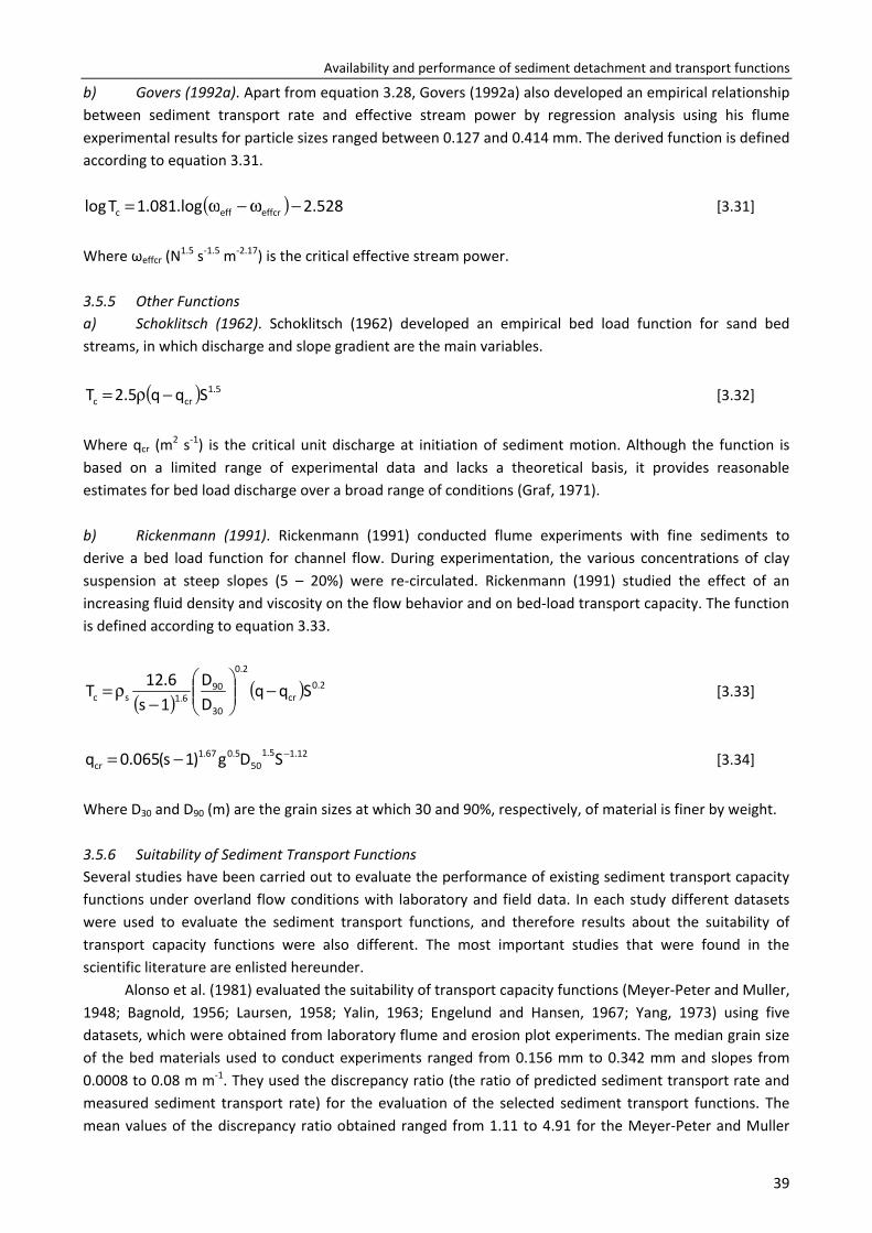
Availability and performance of sediment detachment and transport functions
39
b) Govers (1992a). Apart from equation 3.28, Govers (1992a) also developed an empirical relationship between sediment transport rate and effective stream power by regression analysis using his flume experimental results for particle sizes ranged between 0.127 and 0.414 mm. The derived function is defined according to equation 3.31.
( ) 528.2.log081.1Tlog effcreffc −ω−ω= [3.31]
Where ωeffcr (N1.5 s-1.5 m-2.17) is the critical effective stream power.
3.5.5 Other Functions a) Schoklitsch (1962). Schoklitsch (1962) developed an empirical bed load function for sand bed streams, in which discharge and slope gradient are the main variables.
( ) 5.1crc Sqq5.2T −ρ= [3.32]
Where qcr (m2 s-1) is the critical unit discharge at initiation of sediment motion. Although the function is based on a limited range of experimental data and lacks a theoretical basis, it provides reasonable estimates for bed load discharge over a broad range of conditions (Graf, 1971).
b) Rickenmann (1991). Rickenmann (1991) conducted flume experiments with fine sediments to derive a bed load function for channel flow. During experimentation, the various concentrations of clay suspension at steep slopes (5 – 20%) were re-circulated. Rickenmann (1991) studied the effect of an increasing fluid density and viscosity on the flow behavior and on bed-load transport capacity. The function is defined according to equation 3.33.
( ) ( ) 2.0cr
2.0
30
906.1sc Sqq
DD
1s6.12T −
−
ρ= [3.33]
12.15.1
505.067.1
cr SDg)1s(065.0q −−= [3.34]
Where D30 and D90 (m) are the grain sizes at which 30 and 90%, respectively, of material is finer by weight.
3.5.6 Suitability of Sediment Transport Functions Several studies have been carried out to evaluate the performance of existing sediment transport capacity functions under overland flow conditions with laboratory and field data. In each study different datasets were used to evaluate the sediment transport functions, and therefore results about the suitability of transport capacity functions were also different. The most important studies that were found in the scientific literature are enlisted hereunder.
Alonso et al. (1981) evaluated the suitability of transport capacity functions (Meyer-Peter and Muller, 1948; Bagnold, 1956; Laursen, 1958; Yalin, 1963; Engelund and Hansen, 1967; Yang, 1973) using five datasets, which were obtained from laboratory flume and erosion plot experiments. The median grain size of the bed materials used to conduct experiments ranged from 0.156 mm to 0.342 mm and slopes from 0.0008 to 0.08 m m-1. They used the discrepancy ratio (the ratio of predicted sediment transport rate and measured sediment transport rate) for the evaluation of the selected sediment transport functions. The mean values of the discrepancy ratio obtained ranged from 1.11 to 4.91 for the Meyer-Peter and Muller
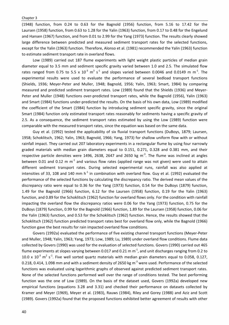
Chapter 3
40
(1948) function, from 0.24 to 0.63 for the Bagnold (1956) function, from 5.16 to 17.42 for the Laursen (1958) function, from 0.63 to 1.28 for the Yalin (1963) function, from 0.17 to 0.48 for the Engelund and Hansen (1967) function, and from 0.01 to 2.99 for the Yang (1973) function. The results clearly showed large difference between predicted and measured sediment transport rates for the selected functions, except for the Yalin (1963) function. Therefore, Alonso et al. (1981) recommended the Yalin (1963) function to estimate sediment transport rate in overland flows.
Low (1989) carried out 187 flume experiments with light weight plastic particles of median grain diameter equal to 3.5 mm and sediment specific gravity varied between 1.0 and 2.5. The simulated flow rates ranged from 0.75 to 5.5 x 10⁻³ m3 s-1 and slopes varied between 0.0046 and 0.0149 m m-1. The experimental results were used to evaluate the performance of several bedload transport functions (Shields, 1936; Meyer-Peter and Muller, 1948; Bagnold, 1956; Yalin, 1963; Smart, 1984) by comparing measured and predicted sediment transport rates. Low (1989) found that the Shields (1936) and Meyer-Peter and Muller (1948) functions over-predicted transport rates, while the Bagnold (1956), Yalin (1963) and Smart (1984) functions under-predicted the results. On the basis of his own data, Low (1989) modified the coefficient of the Smart (1984) function by introducing sediment specific gravity, since the original Smart (1984) function only estimated transport rates reasonably for sediments having a specific gravity of 2.5. As a consequence, the sediment transport rates estimated by using the Low (1989) function were comparable with the measured transport rates, since the equation was based on the same data.
Guy et al. (1992) tested the applicability of six fluvial transport functions (DuBoys, 1879; Laursen, 1958; Schoklitsch, 1962; Yalin, 1963; Bagnold, 1966; Yang, 1973) for shallow uniform flow with or without rainfall impact. They carried out 207 laboratory experiments in a rectangular flume by using four narrowly graded materials with median grain diameters equal to 0.151, 0.271, 0.328 and 0.381 mm, and their respective particle densities were 1496, 2638, 2647 and 2650 kg m-3. The flume was inclined at angles between 0.01 and 0.12 m m-1 and various flow rates (applied range was not given) were used to attain different sediment transport rates. During selected experimental runs, rainfall was also applied at intensities of 33, 108 and 140 mm h-1 in combination with overland flow. Guy et al. (1992) evaluated the performance of the selected functions by calculating the discrepancy ratio. The derived mean values of the discrepancy ratio were equal to 0.36 for the Yang (1973) function, 0.54 for the DuBoys (1879) function, 1.49 for the Bagnold (1966) function, 6.12 for the Laursen (1958) function, 0.19 for the Yalin (1963) function, and 0.89 for the Schoklitsch (1962) function for overland flows only. For the condition with rainfall impacting the overland flow the discrepancy ratios were 0.06 for the Yang (1973) function, 0.75 for the DuBoys (1879) function, 0.99 for the Bagnold (1966) function, 1.89 for the Laursen (1958) function, 0.06 for the Yalin (1963) function, and 0.53 for the Schoklitsch (1962) function. Hence, the results showed that the Schoklitsch (1962) function predicted transport rates best for overland flow only, while the Bagnold (1966) function gave the best results for rain impacted overland flow conditions.
Govers (1992a) evaluated the performance of five existing channel transport functions (Meyer-Peter and Muller, 1948; Yalin, 1963; Yang, 1973; Low, 1989; Lu, 1989) under overland flow conditions. Flume data collected by Govers (1990) was used for the evaluation of selected functions. Govers (1990) carried out 465 flume experiments at slopes varying between 0.017 and 0.21 m m-1, and unit discharges ranging from 0.2 to 10.0 x 10⁻³ m2 s-1. Five well sorted quartz materials with median grain diameters equal to 0.058, 0.127, 0.218, 0.414, 1.098 mm and with a sediment density of 2650 kg m-3 were used. Performance of the selected functions was evaluated using logarithmic graphs of observed against predicted sediment transport rates. None of the selected functions performed well over the range of conditions tested. The best performing function was the one of Low (1989). On the basis of the dataset used, Govers (1992a) developed new empirical functions (equations 3.28 and 3.31) and checked their performance on datasets collected by Kramer and Meyer (1969), Meyer et al. (1983), Rauws (1984), Riley and Gorey (1988) and Aziz and Scott (1989). Govers (1992a) found that the proposed functions exhibited better agreement of results with other
Availability and performance of sediment detachment and transport functions
41
datasets. He also recommended that the new developed functions can be used in erosion models, especially for rill erosion.
Hessel and Jetten (2007) checked the suitability of eight sediment transport functions (Schoklitsch, 1962; Yalin, 1963; Yang, 1973; Bagnold, 1980; Low, 1989; Govers, 1990; Rickenmann, 1991; Abrahams et al., 2001) by incorporating them in the LISEM model (De Roo et al., 1996). The model was applied to the Danangou catchment (3.5 Km2) of the Chinese loess plateau, where the soils are mainly erodible silt loams with a median grain diameter equal to 0.035 mm. Discharges were measured for the period from 1998 to 2000 at a weir, which was constructed at the catchment outlet. In this study, slopes were very steep and ranged from 0.5 and 2.5 m m-1. The performance of the selected sediment transport functions was evaluated by comparing the predicted and measured sediment yield at the catchment outlet and also by comparing the predicted and measured total soil loss. Graphical comparison of predicted and measured sediment yield revealed that most of the selected functions like Schoklitsch (1962), Yalin (1963), Bagnold (1980), Low (1989), Rickenmann (1991) and Abrahams et al. (2001) over-predicted the transport rates at steep slopes and under-predicted the transport rates at gentle slopes. Hence, these functions were found to be sensitive to slope angle. The Yang (1973) function over-predicted sediment yield for both mild and steep slopes, because it appeared to be sensitive to sediment particle size. Only the Govers (1990) function performed well because this function showed lower dependency on both slope and grain size. For one particular storm the Govers (1990) function over predicted the total soil loss by only 21%, while all other functions resulted in larger over or under predictions. Therefore, Hessel and Jetten (2007) recommended the use of the Govers (1990) function (equation 3.27) in erosion models, because it gave the best agreement with measured erosion data.
Nord and Esteves (2007) applied the PSEM_2D numerical model on five different texture soils by incorporating four sediment transport functions (Yalin, 1963; Low, 1989; Govers (1992a) Unit Stream Power; Govers (1992a) Effective Stream Power) for rill flows. The selected soils for the experiments included three cohesive sediments (the Pierre, the Collamer, and the Barnes_ND soils with D50 equal to 0.004, 0.014 and 0.028 mm respectively) and two non-cohesive sediments (the Amarillo and the Bonifay soils with D50 equal to 0.23 and 0.31 mm respectively). The slopes ranged from 0.04 to 0.09 m m-1. A pair of identical rills was considered for each soil and the initial shape of a rill was 9.0 m long, 0.5 m wide, and 0.05 m deep with a uniform trapezoidal cross-section. Applied flow discharge in a single rill was 0.66 x 10⁻³ m3 s-1. The predicted sediment loads were compared with the observed sediment loads to evaluate the performance of selected functions. Nord and Esteves (2007) found that the Govers (1992a) Unit Stream Power function (equation 3.28) exhibited the best results for cohesive soils, but all of the selected functions showed poor performance for non-cohesive soils.
3.6 Summary and Conclusions
Given the large number of existing sediment detachment and transport capacity functions, the main questions regarding their application are then: which function will give promising results when and where? Selecting appropriate sediment detachment and sediment transport functions for a particular condition requires the information about their data requirements, complexities involved, assumptions made during derivation and boundary conditions for which they were derived. Therefore as a step towards this understanding, soil detachment and transport capacity functions considered widely in soil erosion modelling were reviewed.
Most of the existing detachment functions were empirically derived by directly relating the detachment capacity with a composite force predictor. In the literature only detachment functions were found that are either based on shear stress or on stream power. In these functions, the soil’s resistance against erosion is represented by a soil erodibility factor, which principally depends on soil characteristics.
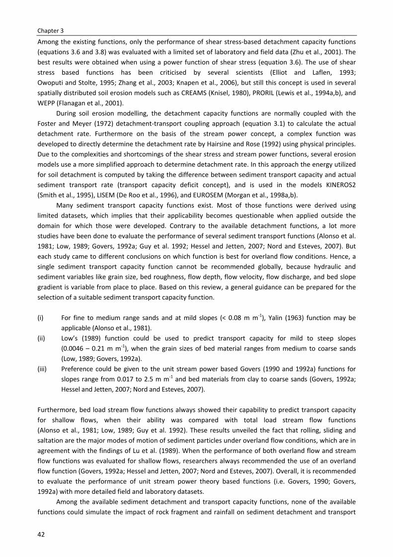
Chapter 3
42
Among the existing functions, only the performance of shear stress-based detachment capacity functions (equations 3.6 and 3.8) was evaluated with a limited set of laboratory and field data (Zhu et al., 2001). The best results were obtained when using a power function of shear stress (equation 3.6). The use of shear stress based functions has been criticised by several scientists (Elliot and Laflen, 1993; Owoputi and Stolte, 1995; Zhang et al., 2003; Knapen et al., 2006), but still this concept is used in several spatially distributed soil erosion models such as CREAMS (Knisel, 1980), PRORIL (Lewis et al., 1994a,b), and WEPP (Flanagan et al., 2001).
During soil erosion modelling, the detachment capacity functions are normally coupled with the Foster and Meyer (1972) detachment-transport coupling approach (equation 3.1) to calculate the actual detachment rate. Furthermore on the basis of the stream power concept, a complex function was developed to directly determine the detachment rate by Hairsine and Rose (1992) using physical principles. Due to the complexities and shortcomings of the shear stress and stream power functions, several erosion models use a more simplified approach to determine detachment rate. In this approach the energy utilized for soil detachment is computed by taking the difference between sediment transport capacity and actual sediment transport rate (transport capacity deficit concept), and is used in the models KINEROS2 (Smith et al., 1995), LISEM (De Roo et al., 1996), and EUROSEM (Morgan et al., 1998a,b).
Many sediment transport capacity functions exist. Most of those functions were derived using limited datasets, which implies that their applicability becomes questionable when applied outside the domain for which those were developed. Contrary to the available detachment functions, a lot more studies have been done to evaluate the performance of several sediment transport functions (Alonso et al. 1981; Low, 1989; Govers, 1992a; Guy et al. 1992; Hessel and Jetten, 2007; Nord and Esteves, 2007). But each study came to different conclusions on which function is best for overland flow conditions. Hence, a single sediment transport capacity function cannot be recommended globally, because hydraulic and sediment variables like grain size, bed roughness, flow depth, flow velocity, flow discharge, and bed slope gradient is variable from place to place. Based on this review, a general guidance can be prepared for the selection of a suitable sediment transport capacity function.
(i) For fine to medium range sands and at mild slopes (< 0.08 m m-1), Yalin (1963) function may be
applicable (Alonso et al., 1981). (ii) Low’s (1989) function could be used to predict transport capacity for mild to steep slopes
(0.0046 – 0.21 m m-1), when the grain sizes of bed material ranges from medium to coarse sands (Low, 1989; Govers, 1992a).
(iii) Preference could be given to the unit stream power based Govers (1990 and 1992a) functions for slopes range from 0.017 to 2.5 m m-1 and bed materials from clay to coarse sands (Govers, 1992a; Hessel and Jetten, 2007; Nord and Esteves, 2007).
Furthermore, bed load stream flow functions always showed their capability to predict transport capacity for shallow flows, when their ability was compared with total load stream flow functions (Alonso et al., 1981; Low, 1989; Guy et al. 1992). These results unveiled the fact that rolling, sliding and saltation are the major modes of motion of sediment particles under overland flow conditions, which are in agreement with the findings of Lu et al. (1989). When the performance of both overland flow and stream flow functions was evaluated for shallow flows, researchers always recommended the use of an overland flow function (Govers, 1992a; Hessel and Jetten, 2007; Nord and Esteves, 2007). Overall, it is recommended to evaluate the performance of unit stream power theory based functions (i.e. Govers, 1990; Govers, 1992a) with more detailed field and laboratory datasets.
Among the available sediment detachment and transport capacity functions, none of the available functions could simulate the impact of rock fragment and rainfall on sediment detachment and transport
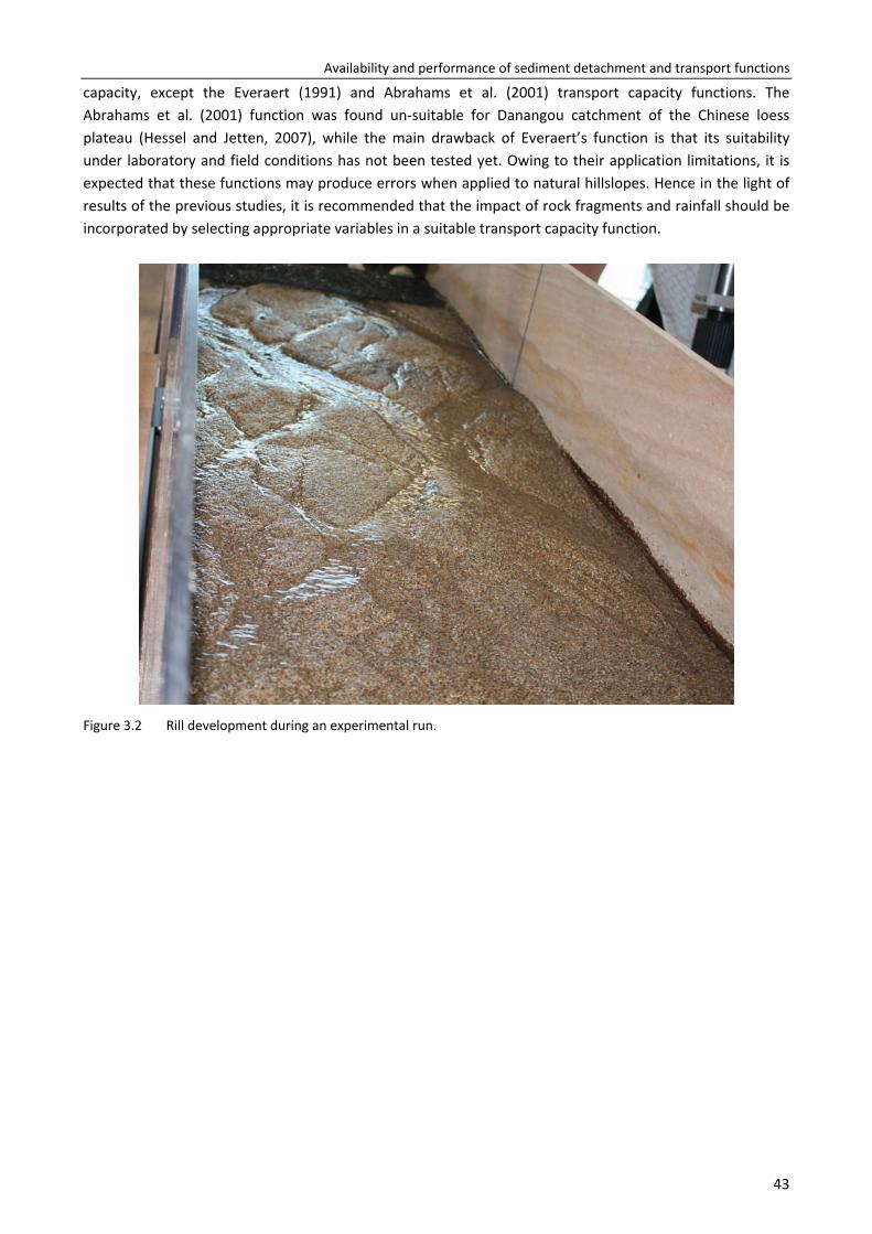
Availability and performance of sediment detachment and transport functions
43
capacity, except the Everaert (1991) and Abrahams et al. (2001) transport capacity functions. The Abrahams et al. (2001) function was found un-suitable for Danangou catchment of the Chinese loess plateau (Hessel and Jetten, 2007), while the main drawback of Everaert’s function is that its suitability under laboratory and field conditions has not been tested yet. Owing to their application limitations, it is expected that these functions may produce errors when applied to natural hillslopes. Hence in the light of results of the previous studies, it is recommended that the impact of rock fragments and rainfall should be incorporated by selecting appropriate variables in a suitable transport capacity function.
Figure 3.2 Rill development during an experimental run.

Chapter 4
Effect of flow discharge and median grain size on mean flow velocity under overland flow
Ali M., Sterk G., Seeger M. and L. Stroosnijder Earth Surface Processes and Landforms (accepted).

47
Effect of flow discharge and median grain size on mean flow velocity under overland flow
Abstract
Precise estimation of mean flow velocity (Umean) is imperative for accurate prediction of hydrographs and sediment yield. For overland flow, Umean is normally estimated by multiplying the dye or salt based velocity measurement with a correction factor (α). A wide range of correction factors is available in the literature, all of which were derived under different experimental conditions. The selection of a suitable α has become a main challenge for accurate mean flow calculations. This study aimed to assess the variability of α with grain size (D50) and slope (S), and to evaluate the dependency of Umean on flow rate (Q), D50 and S by regression analysis. Flume experiments were performed at Q varying from 33 to 1033 x 10-6 m3 s-1, S ranging from 3o to 10o, and D50 ranging from 0.233 to 1.022 mm. Flow velocities were measured directly with the dye tracing technique (Udye), and derived indirectly from flow depth measurements (Udepth). The Udepth measurements were considered as Umean. The derived α (Udepth/Udye) values did not remain constant with sediment size and increase significantly with the increase of D50. The mean α values for 0.230, 0.536, 0.719 and 1.022 mm sands were 0.44, 0.77, 0.82 and 0.82, respectively. Hence, due to the substantial variation of α with D50, no absolute α value is applicable to all hydraulic and sedimentary conditions. However, mean α values for 0.230 and 0.719 mm sands were found comparable with α values available in the literature for similar grain sizes. The influence of Q, S, and D50 on Umean was studied by regression analysis. Regression analysis depicted the significant influence of Q and D50 on Umean, while the effect of slope was found to be non-significant. Comparison of the derived regression equation with five literature datasets showed that the model can predict mean flow velocities in overland flow at a reasonable accuracy as long as the mean velocity in below 0.4 m s-1. At higher velocities the error becomes unacceptably large.
4.1 Introduction
Soil erosion is a main global ecological problem, threatening agricultural production and storage of reservoirs (Lal and Stewart, 1990). Several physically based soil erosion models have been developed to identify the sensitive areas in a catchment. But, the further understanding of the processes involved in soil erosion is still needed to enhance the accuracy of existing models. For this purpose, numerous field and laboratory scale flume studies have been carried out, intended for the accurate assessment of hydraulic and sediment parameters (Abrahams et al., 1986; Abrahams et al., 1996; Takken and Govers, 2000; Dunkerley, 2001). A precise quantification of mean flow velocity under overland flow is important for soil erosion studies in both laboratory and field conditions.
Worldwide, many techniques are being used for the estimation of mean flow velocity under overland flow i.e. magnetic velocimeters and particle imaging velocimetry (Raffel et al., 1998), hot film anemometry (Ayala et al., 2000), the optical tachometer method (Dunkerley, 2003), acoustic doppler velocimetry (Gimenez et al., 2004), salt velocity gauge (Planchon et al., 2005), pulse method (Lei et al., 2005; 2010), dye tracing technique (Abrahams et al., 1986; Takken and Govers, 2000) and salt tracing technique (Abrahams and Atkinson, 1993; Li et al., 1996; Lei et al., 2005). The mean flow velocity can also be estimated indirectly from flow depth measurements (Emmett, 1970; Takken and Govers, 2000). However, each technique is based on certain limitations, because they all were developed in the laboratory under controlled conditions. For example, magnetic velocimeters and acoustic doppler velocimetry methods are only applicable to flow conditions, where flow depths are equal or more than 1.5 cm (Planchon et al., 2005), and
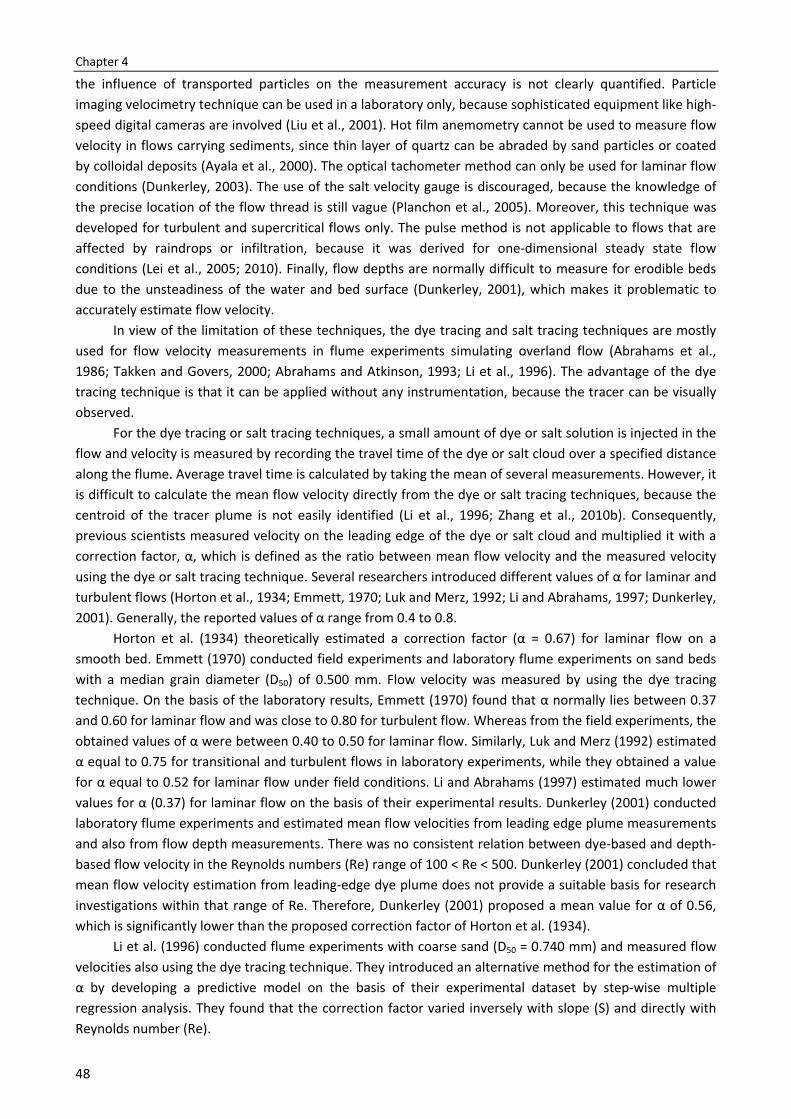
Chapter 4
48
the influence of transported particles on the measurement accuracy is not clearly quantified. Particle imaging velocimetry technique can be used in a laboratory only, because sophisticated equipment like high-speed digital cameras are involved (Liu et al., 2001). Hot film anemometry cannot be used to measure flow velocity in flows carrying sediments, since thin layer of quartz can be abraded by sand particles or coated by colloidal deposits (Ayala et al., 2000). The optical tachometer method can only be used for laminar flow conditions (Dunkerley, 2003). The use of the salt velocity gauge is discouraged, because the knowledge of the precise location of the flow thread is still vague (Planchon et al., 2005). Moreover, this technique was developed for turbulent and supercritical flows only. The pulse method is not applicable to flows that are affected by raindrops or infiltration, because it was derived for one-dimensional steady state flow conditions (Lei et al., 2005; 2010). Finally, flow depths are normally difficult to measure for erodible beds due to the unsteadiness of the water and bed surface (Dunkerley, 2001), which makes it problematic to accurately estimate flow velocity.
In view of the limitation of these techniques, the dye tracing and salt tracing techniques are mostly used for flow velocity measurements in flume experiments simulating overland flow (Abrahams et al., 1986; Takken and Govers, 2000; Abrahams and Atkinson, 1993; Li et al., 1996). The advantage of the dye tracing technique is that it can be applied without any instrumentation, because the tracer can be visually observed.
For the dye tracing or salt tracing techniques, a small amount of dye or salt solution is injected in the flow and velocity is measured by recording the travel time of the dye or salt cloud over a specified distance along the flume. Average travel time is calculated by taking the mean of several measurements. However, it is difficult to calculate the mean flow velocity directly from the dye or salt tracing techniques, because the centroid of the tracer plume is not easily identified (Li et al., 1996; Zhang et al., 2010b). Consequently, previous scientists measured velocity on the leading edge of the dye or salt cloud and multiplied it with a correction factor, α, which is defined as the ratio between mean flow velocity and the measured velocity using the dye or salt tracing technique. Several researchers introduced different values of α for laminar and turbulent flows (Horton et al., 1934; Emmett, 1970; Luk and Merz, 1992; Li and Abrahams, 1997; Dunkerley, 2001). Generally, the reported values of α range from 0.4 to 0.8.
Horton et al. (1934) theoretically estimated a correction factor (α = 0.67) for laminar flow on a smooth bed. Emmett (1970) conducted field experiments and laboratory flume experiments on sand beds with a median grain diameter (D50) of 0.500 mm. Flow velocity was measured by using the dye tracing technique. On the basis of the laboratory results, Emmett (1970) found that α normally lies between 0.37 and 0.60 for laminar flow and was close to 0.80 for turbulent flow. Whereas from the field experiments, the obtained values of α were between 0.40 to 0.50 for laminar flow. Similarly, Luk and Merz (1992) estimated α equal to 0.75 for transitional and turbulent flows in laboratory experiments, while they obtained a value for α equal to 0.52 for laminar flow under field conditions. Li and Abrahams (1997) estimated much lower values for α (0.37) for laminar flow on the basis of their experimental results. Dunkerley (2001) conducted laboratory flume experiments and estimated mean flow velocities from leading edge plume measurements and also from flow depth measurements. There was no consistent relation between dye-based and depth-based flow velocity in the Reynolds numbers (Re) range of 100 < Re < 500. Dunkerley (2001) concluded that mean flow velocity estimation from leading-edge dye plume does not provide a suitable basis for research investigations within that range of Re. Therefore, Dunkerley (2001) proposed a mean value for α of 0.56, which is significantly lower than the proposed correction factor of Horton et al. (1934).
Li et al. (1996) conducted flume experiments with coarse sand (D50 = 0.740 mm) and measured flow velocities also using the dye tracing technique. They introduced an alternative method for the estimation of α by developing a predictive model on the basis of their experimental dataset by step-wise multiple regression analysis. They found that the correction factor varied inversely with slope (S) and directly with Reynolds number (Re).
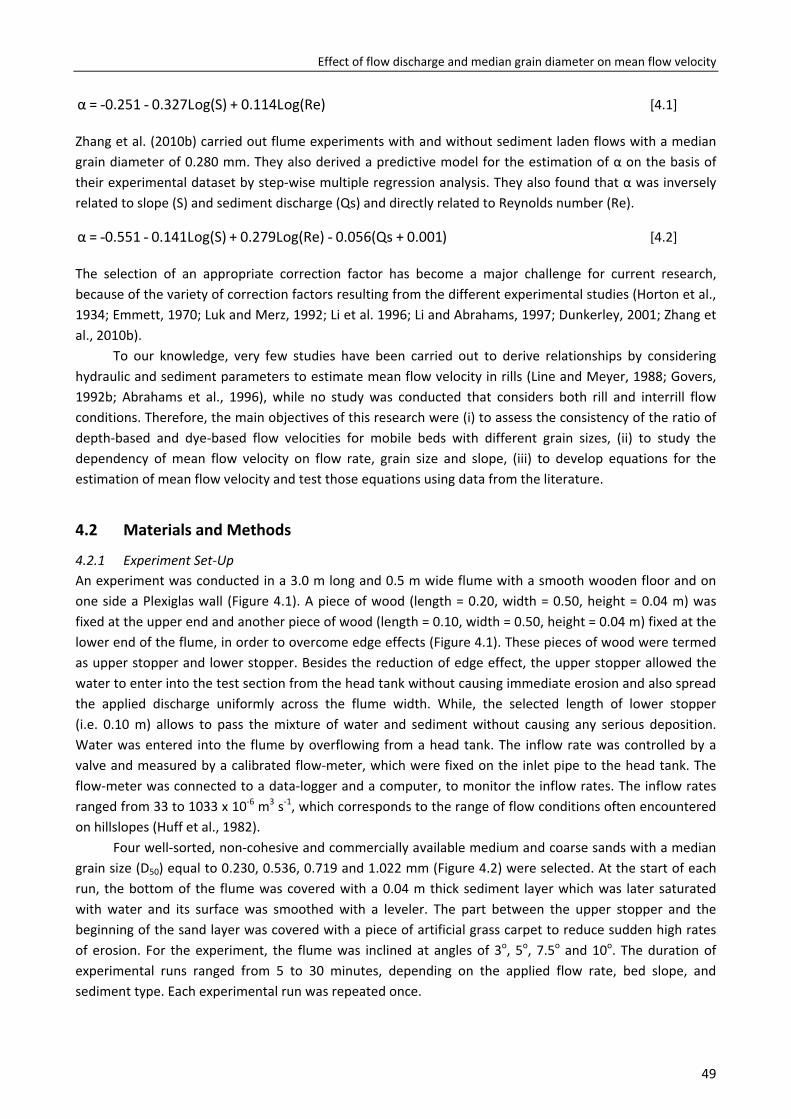
Effect of flow discharge and median grain diameter on mean flow velocity
49
og(Re)0.114L+og(S)0.327L0.251=α -- [4.1]
Zhang et al. (2010b) carried out flume experiments with and without sediment laden flows with a median grain diameter of 0.280 mm. They also derived a predictive model for the estimation of α on the basis of their experimental dataset by step-wise multiple regression analysis. They also found that α was inversely related to slope (S) and sediment discharge (Qs) and directly related to Reynolds number (Re).
)0.001+(Qs0.056og(Re)0.279L+og(S)0.141L0.551=α --- [4.2]
The selection of an appropriate correction factor has become a major challenge for current research, because of the variety of correction factors resulting from the different experimental studies (Horton et al., 1934; Emmett, 1970; Luk and Merz, 1992; Li et al. 1996; Li and Abrahams, 1997; Dunkerley, 2001; Zhang et al., 2010b).
To our knowledge, very few studies have been carried out to derive relationships by considering hydraulic and sediment parameters to estimate mean flow velocity in rills (Line and Meyer, 1988; Govers, 1992b; Abrahams et al., 1996), while no study was conducted that considers both rill and interrill flow conditions. Therefore, the main objectives of this research were (i) to assess the consistency of the ratio of depth-based and dye-based flow velocities for mobile beds with different grain sizes, (ii) to study the dependency of mean flow velocity on flow rate, grain size and slope, (iii) to develop equations for the estimation of mean flow velocity and test those equations using data from the literature.
4.2 Materials and Methods
4.2.1 Experiment Set-Up An experiment was conducted in a 3.0 m long and 0.5 m wide flume with a smooth wooden floor and on one side a Plexiglas wall (Figure 4.1). A piece of wood (length = 0.20, width = 0.50, height = 0.04 m) was fixed at the upper end and another piece of wood (length = 0.10, width = 0.50, height = 0.04 m) fixed at the lower end of the flume, in order to overcome edge effects (Figure 4.1). These pieces of wood were termed as upper stopper and lower stopper. Besides the reduction of edge effect, the upper stopper allowed the water to enter into the test section from the head tank without causing immediate erosion and also spread the applied discharge uniformly across the flume width. While, the selected length of lower stopper (i.e. 0.10 m) allows to pass the mixture of water and sediment without causing any serious deposition. Water was entered into the flume by overflowing from a head tank. The inflow rate was controlled by a valve and measured by a calibrated flow-meter, which were fixed on the inlet pipe to the head tank. The flow-meter was connected to a data-logger and a computer, to monitor the inflow rates. The inflow rates ranged from 33 to 1033 x 10-6 m3 s-1, which corresponds to the range of flow conditions often encountered on hillslopes (Huff et al., 1982).
Four well-sorted, non-cohesive and commercially available medium and coarse sands with a median grain size (D50) equal to 0.230, 0.536, 0.719 and 1.022 mm (Figure 4.2) were selected. At the start of each run, the bottom of the flume was covered with a 0.04 m thick sediment layer which was later saturated with water and its surface was smoothed with a leveler. The part between the upper stopper and the beginning of the sand layer was covered with a piece of artificial grass carpet to reduce sudden high rates of erosion. For the experiment, the flume was inclined at angles of 3o, 5o, 7.5o and 10o. The duration of experimental runs ranged from 5 to 30 minutes, depending on the applied flow rate, bed slope, and sediment type. Each experimental run was repeated once.
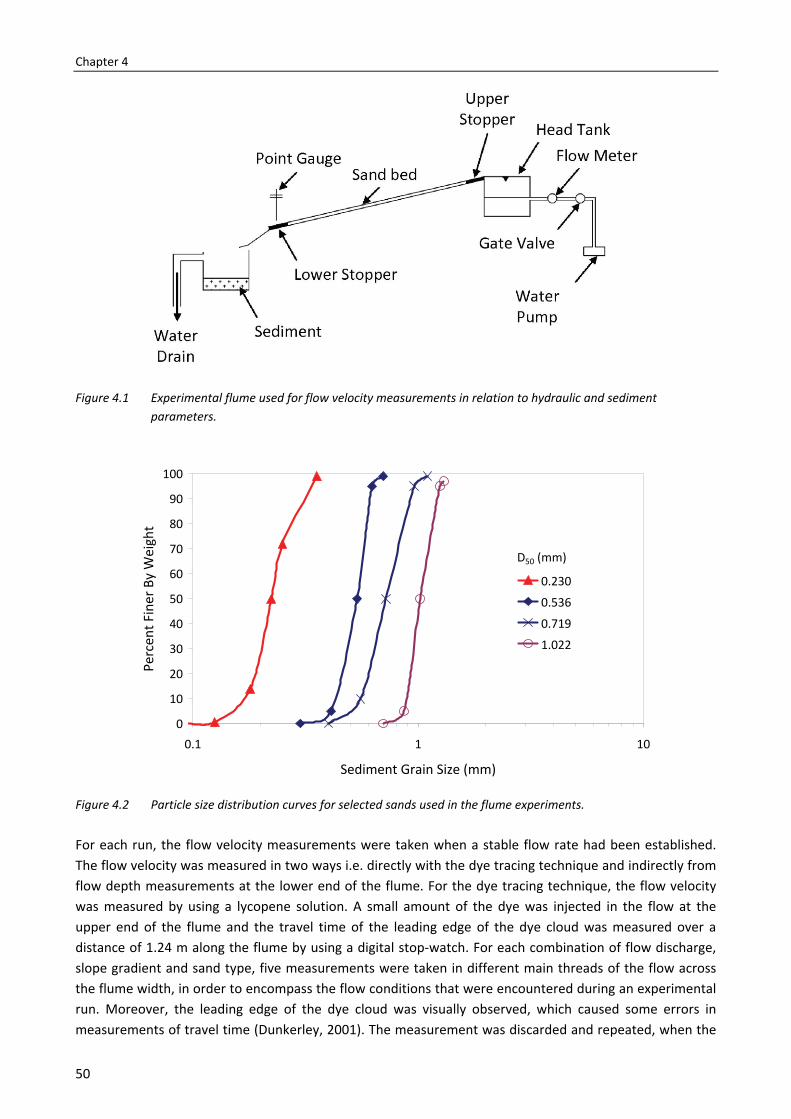
Chapter 4
50
Figure 4.1 Experimental flume used for flow velocity measurements in relation to hydraulic and sediment parameters.
Figure 4.2 Particle size distribution curves for selected sands used in the flume experiments.
For each run, the flow velocity measurements were taken when a stable flow rate had been established. The flow velocity was measured in two ways i.e. directly with the dye tracing technique and indirectly from flow depth measurements at the lower end of the flume. For the dye tracing technique, the flow velocity was measured by using a lycopene solution. A small amount of the dye was injected in the flow at the upper end of the flume and the travel time of the leading edge of the dye cloud was measured over a distance of 1.24 m along the flume by using a digital stop-watch. For each combination of flow discharge, slope gradient and sand type, five measurements were taken in different main threads of the flow across the flume width, in order to encompass the flow conditions that were encountered during an experimental run. Moreover, the leading edge of the dye cloud was visually observed, which caused some errors in measurements of travel time (Dunkerley, 2001). The measurement was discarded and repeated, when the
0
10
20
30
40
50
60
70
80
90
100
0.1 1 10
Sediment Grain Size (mm)
Perc
ent F
iner
By
Wei
ght
0.230
0.536
0.719
1.022
D50 (mm)
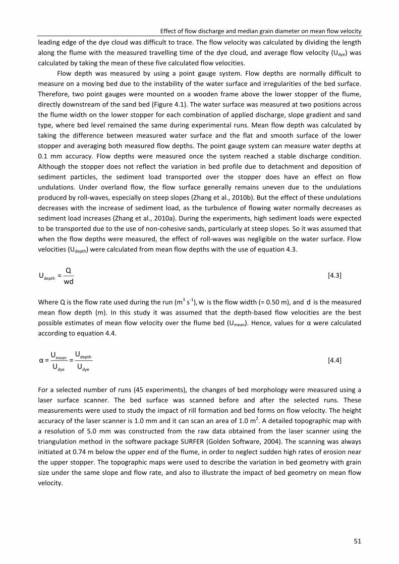
Effect of flow discharge and median grain diameter on mean flow velocity
51
leading edge of the dye cloud was difficult to trace. The flow velocity was calculated by dividing the length along the flume with the measured travelling time of the dye cloud, and average flow velocity (Udye) was calculated by taking the mean of these five calculated flow velocities.
Flow depth was measured by using a point gauge system. Flow depths are normally difficult to measure on a moving bed due to the instability of the water surface and irregularities of the bed surface. Therefore, two point gauges were mounted on a wooden frame above the lower stopper of the flume, directly downstream of the sand bed (Figure 4.1). The water surface was measured at two positions across the flume width on the lower stopper for each combination of applied discharge, slope gradient and sand type, where bed level remained the same during experimental runs. Mean flow depth was calculated by taking the difference between measured water surface and the flat and smooth surface of the lower stopper and averaging both measured flow depths. The point gauge system can measure water depths at 0.1 mm accuracy. Flow depths were measured once the system reached a stable discharge condition. Although the stopper does not reflect the variation in bed profile due to detachment and deposition of sediment particles, the sediment load transported over the stopper does have an effect on flow undulations. Under overland flow, the flow surface generally remains uneven due to the undulations produced by roll-waves, especially on steep slopes (Zhang et al., 2010b). But the effect of these undulations decreases with the increase of sediment load, as the turbulence of flowing water normally decreases as sediment load increases (Zhang et al., 2010a). During the experiments, high sediment loads were expected to be transported due to the use of non-cohesive sands, particularly at steep slopes. So it was assumed that when the flow depths were measured, the effect of roll-waves was negligible on the water surface. Flow velocities (Udepth) were calculated from mean flow depths with the use of equation 4.3.
wdQ=Udepth [4.3]
Where Q is the flow rate used during the run (m3 s-1), w is the flow width (= 0.50 m), and d is the measured mean flow depth (m). In this study it was assumed that the depth-based flow velocities are the best possible estimates of mean flow velocity over the flume bed (Umean). Hence, values for α were calculated according to equation 4.4.
dye
depth
dye
mean
UU
=UU
=α [4.4]
For a selected number of runs (45 experiments), the changes of bed morphology were measured using a laser surface scanner. The bed surface was scanned before and after the selected runs. These measurements were used to study the impact of rill formation and bed forms on flow velocity. The height accuracy of the laser scanner is 1.0 mm and it can scan an area of 1.0 m2. A detailed topographic map with a resolution of 5.0 mm was constructed from the raw data obtained from the laser scanner using the triangulation method in the software package SURFER (Golden Software, 2004). The scanning was always initiated at 0.74 m below the upper end of the flume, in order to neglect sudden high rates of erosion near the upper stopper. The topographic maps were used to describe the variation in bed geometry with grain size under the same slope and flow rate, and also to illustrate the impact of bed geometry on mean flow velocity.
Chapter 4
52
The variation of ratios of depth-based and dye-based flow velocities (= α) were used to study the impact of grain size, slope and bed geometry on the mean flow velocity (Umean). Moreover, linear regression analysis was carried out to develop models between mean flow velocity and easily measurable hydraulic and sediment parameters. The regression analysis was undertaken in PASW statistics 17 software (SPSS Inc., 2009). To evaluate the performance of the proposed models, use was made of the coefficient of
determination (R2), the discrepancy ratio (obs
cal
UU
), the Nash and Sutcliffe (1970) model efficiency (Ef).
( )( )∑
∑-
-- 2
obsobs
2calobs
fUU
UU1=E [4.5]
The relative root mean square error (RRMSE) can be calculated with the use of equation 4.6.
( )
obs
2calobs
U
UUn1
=RRMSE∑ -
[4.6]
And the error between measured and predicted flow velocities (E) can be calculated with the use of equation 4.7.
[ ]calobs UU=E - [4.7]
Where Uobs is the observed flow velocity, Ucal is the model calculated velocity, obsU is the mean of observed
flow velocities, and n is the number of observations. Five data-sets (Aziz and Scott, 1989; Li et al., 1996; Li and Abrahams, 1997; Hu and Abrahams, 2005; Zhang et al., 2010b) were selected from the literature for the validation of the derived regression equations. The overview of the selected datasets is presented in Table 4.1. The sediment sizes and slopes used to conduct these experiments were comparable with our dataset. But in those cases, the flow beds were fixed and the sediments were introduced into the water by means of a sediment hopper. As a result, they could apply higher flow rates, resulting in generally higher flow velocities (Table 4.1).
Table 4.1 Overview of literature datasets.
Author(s) No. of
Experiments D50 mm
Slope (m m-1)
Flow Rate (10-6 m3 s-1)
Reynolds Number
Aziz and Scott (1989) 96 0.285–1.015 0.03–0.10 377 – 1082 6600 – 18850
Li et al. (1996) 40 0.740 0.047 – 0.174 206 – 1403 1902 - 12606
Li and Abrahams (1997) 105 0.740 0.021 – 0.096 68 – 1469 583 - 12998
Hu and Abrahams (2005) 38 0.740 & 1.160 0.051 & 0.114 272 – 1471 2500 – 12500
Zhang et al. (2010b) 20 0.280 0.087 – 0.342 264 – 2104 1061 – 18990
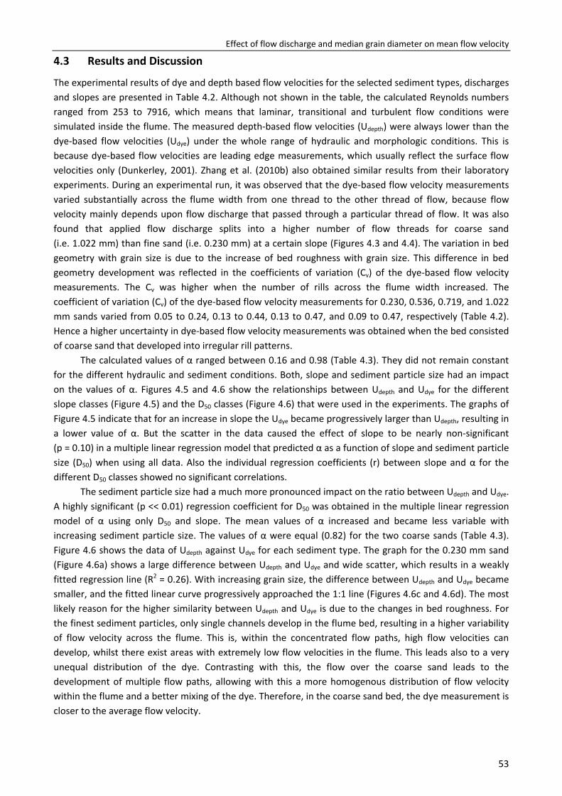
Effect of flow discharge and median grain diameter on mean flow velocity
53
4.3 Results and Discussion
The experimental results of dye and depth based flow velocities for the selected sediment types, discharges and slopes are presented in Table 4.2. Although not shown in the table, the calculated Reynolds numbers ranged from 253 to 7916, which means that laminar, transitional and turbulent flow conditions were simulated inside the flume. The measured depth-based flow velocities (Udepth) were always lower than the dye-based flow velocities (Udye) under the whole range of hydraulic and morphologic conditions. This is because dye-based flow velocities are leading edge measurements, which usually reflect the surface flow velocities only (Dunkerley, 2001). Zhang et al. (2010b) also obtained similar results from their laboratory experiments. During an experimental run, it was observed that the dye-based flow velocity measurements varied substantially across the flume width from one thread to the other thread of flow, because flow velocity mainly depends upon flow discharge that passed through a particular thread of flow. It was also found that applied flow discharge splits into a higher number of flow threads for coarse sand (i.e. 1.022 mm) than fine sand (i.e. 0.230 mm) at a certain slope (Figures 4.3 and 4.4). The variation in bed geometry with grain size is due to the increase of bed roughness with grain size. This difference in bed geometry development was reflected in the coefficients of variation (Cv) of the dye-based flow velocity measurements. The Cv was higher when the number of rills across the flume width increased. The coefficient of variation (Cv) of the dye-based flow velocity measurements for 0.230, 0.536, 0.719, and 1.022 mm sands varied from 0.05 to 0.24, 0.13 to 0.44, 0.13 to 0.47, and 0.09 to 0.47, respectively (Table 4.2). Hence a higher uncertainty in dye-based flow velocity measurements was obtained when the bed consisted of coarse sand that developed into irregular rill patterns.
The calculated values of α ranged between 0.16 and 0.98 (Table 4.3). They did not remain constant for the different hydraulic and sediment conditions. Both, slope and sediment particle size had an impact on the values of α. Figures 4.5 and 4.6 show the relationships between Udepth and Udye for the different slope classes (Figure 4.5) and the D50 classes (Figure 4.6) that were used in the experiments. The graphs of Figure 4.5 indicate that for an increase in slope the Udye became progressively larger than Udepth, resulting in a lower value of α. But the scatter in the data caused the effect of slope to be nearly non-significant (p = 0.10) in a multiple linear regression model that predicted α as a function of slope and sediment particle size (D50) when using all data. Also the individual regression coefficients (r) between slope and α for the different D50 classes showed no significant correlations.
The sediment particle size had a much more pronounced impact on the ratio between Udepth and Udye. A highly significant (p << 0.01) regression coefficient for D50 was obtained in the multiple linear regression model of α using only D50 and slope. The mean values of α increased and became less variable with increasing sediment particle size. The values of α were equal (0.82) for the two coarse sands (Table 4.3). Figure 4.6 shows the data of Udepth against Udye for each sediment type. The graph for the 0.230 mm sand (Figure 4.6a) shows a large difference between Udepth and Udye and wide scatter, which results in a weakly fitted regression line (R2 = 0.26). With increasing grain size, the difference between Udepth and Udye became smaller, and the fitted linear curve progressively approached the 1:1 line (Figures 4.6c and 4.6d). The most likely reason for the higher similarity between Udepth and Udye is due to the changes in bed roughness. For the finest sediment particles, only single channels develop in the flume bed, resulting in a higher variability of flow velocity across the flume. This is, within the concentrated flow paths, high flow velocities can develop, whilst there exist areas with extremely low flow velocities in the flume. This leads also to a very unequal distribution of the dye. Contrasting with this, the flow over the coarse sand leads to the development of multiple flow paths, allowing with this a more homogenous distribution of flow velocity within the flume and a better mixing of the dye. Therefore, in the coarse sand bed, the dye measurement is closer to the average flow velocity.
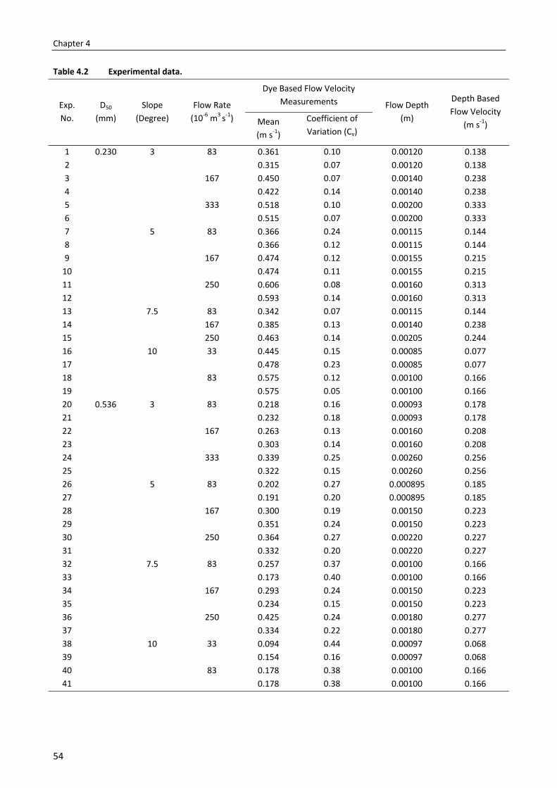
Chapter 4
54
Table 4.2 Experimental data.
Exp. No.
D50
(mm) Slope
(Degree) Flow Rate
(10-6 m3 s-1)
Dye Based Flow Velocity Measurements Flow Depth
(m)
Depth Based Flow Velocity
(m s-1) Mean (m s-1)
Coefficient of Variation (Cv)
1 0.230 3 83 0.361 0.10 0.00120 0.1382 0.315 0.07 0.00120 0.138 3 167 0.450 0.07 0.00140 0.2384 0.422 0.14 0.00140 0.2385 333 0.518 0.10 0.00200 0.333 6 0.515 0.07 0.00200 0.3337 5 83 0.366 0.24 0.00115 0.1448 0.366 0.12 0.00115 0.144 9 167 0.474 0.12 0.00155 0.215
10 0.474 0.11 0.00155 0.21511 250 0.606 0.08 0.00160 0.313 12 0.593 0.14 0.00160 0.31313 7.5 83 0.342 0.07 0.00115 0.14414 167 0.385 0.13 0.00140 0.238 15 250 0.463 0.14 0.00205 0.24416 10 33 0.445 0.15 0.00085 0.07717 0.478 0.23 0.00085 0.077 18 83 0.575 0.12 0.00100 0.16619 0.575 0.05 0.00100 0.16620 0.536 3 83 0.218 0.16 0.00093 0.178 21 0.232 0.18 0.00093 0.17822 167 0.263 0.13 0.00160 0.20823 0.303 0.14 0.00160 0.208 24 333 0.339 0.25 0.00260 0.25625 0.322 0.15 0.00260 0.25626 5 83 0.202 0.27 0.000895 0.185 27 0.191 0.20 0.000895 0.18528 167 0.300 0.19 0.00150 0.22329 0.351 0.24 0.00150 0.223 30 250 0.364 0.27 0.00220 0.22731 0.332 0.20 0.00220 0.22732 7.5 83 0.257 0.37 0.00100 0.166 33 0.173 0.40 0.00100 0.16634 167 0.293 0.24 0.00150 0.22335 0.234 0.15 0.00150 0.223 36 250 0.425 0.24 0.00180 0.27737 0.334 0.22 0.00180 0.27738 10 33 0.094 0.44 0.00097 0.068 39 0.154 0.16 0.00097 0.06840 83 0.178 0.38 0.00100 0.16641 0.178 0.38 0.00100 0.166
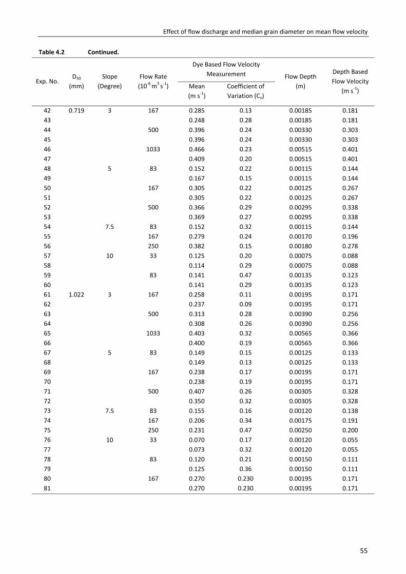
Effect of flow discharge and median grain diameter on mean flow velocity
55
Table 4.2 Continued.
Exp. No. D50
(mm) Slope
(Degree) Flow Rate
(10-6 m3 s-1)
Dye Based Flow Velocity Measurement Flow Depth
(m)
Depth Based Flow Velocity
(m s-1) Mean (m s-1)
Coefficient of Variation (Cv)
42 0.719 3 167 0.285 0.13 0.00185 0.18143 0.248 0.28 0.00185 0.181 44 500 0.396 0.24 0.00330 0.30345 0.396 0.24 0.00330 0.30346 1033 0.466 0.23 0.00515 0.401 47 0.409 0.20 0.00515 0.40148 5 83 0.152 0.22 0.00115 0.14449 0.167 0.15 0.00115 0.144 50 167 0.305 0.22 0.00125 0.26751 0.305 0.22 0.00125 0.26752 500 0.366 0.29 0.00295 0.338 53 0.369 0.27 0.00295 0.33854 7.5 83 0.152 0.32 0.00115 0.14455 167 0.279 0.24 0.00170 0.196 56 250 0.382 0.15 0.00180 0.27857 10 33 0.125 0.20 0.00075 0.08858 0.114 0.29 0.00075 0.088 59 83 0.141 0.47 0.00135 0.12360 0.141 0.29 0.00135 0.12361 1.022 3 167 0.258 0.11 0.00195 0.171 62 0.237 0.09 0.00195 0.17163 500 0.313 0.28 0.00390 0.25664 0.308 0.26 0.00390 0.256 65 1033 0.403 0.32 0.00565 0.36666 0.400 0.19 0.00565 0.36667 5 83 0.149 0.15 0.00125 0.133 68 0.149 0.13 0.00125 0.13369 167 0.238 0.17 0.00195 0.17170 0.238 0.19 0.00195 0.171 71 500 0.407 0.26 0.00305 0.32872 0.350 0.32 0.00305 0.32873 7.5 83 0.155 0.16 0.00120 0.138 74 167 0.206 0.34 0.00175 0.19175 250 0.231 0.47 0.00250 0.20076 10 33 0.070 0.17 0.00120 0.055 77 0.073 0.32 0.00120 0.05578 83 0.120 0.21 0.00150 0.11179 0.125 0.36 0.00150 0.111 80 167 0.270 0.230 0.00195 0.17181 0.270 0.230 0.00195 0.171
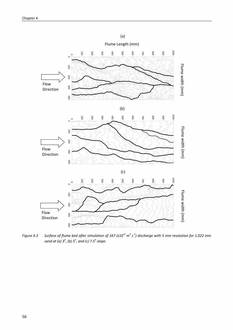
Chapter 4
56
Figure 4.3 Surface of flume bed after simulation of 167 (x10-6 m3 s-1) discharge with 5 mm resolution for 1.022 mm sand at (a) 3o, (b) 5o, and (c) 7.5o slope.
(a)
0100
200300
4000
100
200
300
400
500
600
700
800
900
1000
Flume w
idth (mm
) Flum
e width (m
m)
Flow Direction
Flume w
idth (mm
)
0100
200300
4000
100
200
300
400
500
600
700
800
900
1000
0100
200300
4000
100
200
300
400
500
600
700
800
900
1000
Flume Length (mm)
Flow Direction
Flow Direction
(b)
(c)
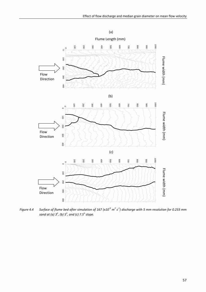
Effect of flow discharge and median grain diameter on mean flow velocity
57
Figure 4.4 Surface of flume bed after simulation of 167 (x10-6 m3 s-1) discharge with 5 mm resolution for 0.233 mm sand at (a) 3o, (b) 5o, and (c) 7.5o slope.
(a)
Flume w
idth (mm
) Flum
e width (m
m)
Flow Direction
Flume w
idth (mm
) Flume Length (mm)
Flow Direction
Flow Direction
(b)
(c)
0100
200300
4000
100
200
300
400
500
600
700
800
900
1000
0100
200300
4000
100
200
300
400
500
600
700
800
900
1000
0100
200300
4000
100
200
300
400
500
600
700
800
900
1000
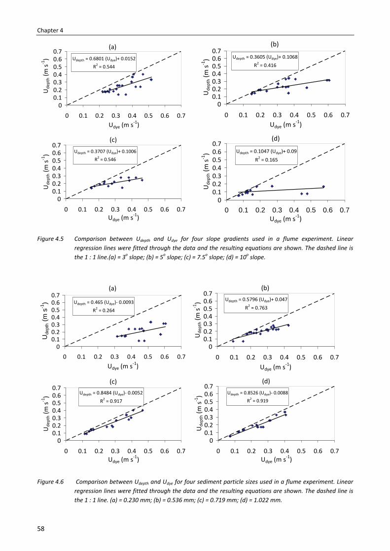
Chapter 4
58
Figure 4.5 Comparison between Udepth and Udye for four slope gradients used in a flume experiment. Linear regression lines were fitted through the data and the resulting equations are shown. The dashed line is the 1 : 1 line.(a) = 3o slope; (b) = 5o slope; (c) = 7.5o slope; (d) = 10o slope.
Figure 4.6 Comparison between Udepth and Udye for four sediment particle sizes used in a flume experiment. Linear
regression lines were fitted through the data and the resulting equations are shown. The dashed line is the 1 : 1 line. (a) = 0.230 mm; (b) = 0.536 mm; (c) = 0.719 mm; (d) = 1.022 mm.
(a)
Udepth = 0.6801 (Udye)+ 0.0152R2 = 0.544
00.10.20.30.40.50.60.7
0 0.1 0.2 0.3 0.4 0.5 0.6 0.7Udye (m s-1)
Ude
pth (
m s-1
)(b)
Udepth = 0.3605 (Udye)+ 0.1068R2 = 0.416
00.10.20.30.40.50.60.7
0 0.1 0.2 0.3 0.4 0.5 0.6 0.7Udye (m s-1)
Ude
pth (
m s-1
)
(c)Udepth = 0.3707 (Udye)+ 0.1006
R2 = 0.546
00.10.20.30.40.50.60.7
0 0.1 0.2 0.3 0.4 0.5 0.6 0.7Udye (m s-1)
Ude
pth (
m s-1
)
(d)
Udepth = 0.1047 (Udye)+ 0.09R2 = 0.165
00.10.20.30.40.50.60.7
0 0.1 0.2 0.3 0.4 0.5 0.6 0.7Udye (m s-1)
Ude
pth (
m s-1
)
(a)
Udepth = 0.465 (Udye)- 0.0093R2 = 0.264
00.10.20.30.40.50.60.7
0 0.1 0.2 0.3 0.4 0.5 0.6 0.7Udye (m s-1)
Ude
pth (
m s
-1)
(b)Udepth = 0.5796 (Udye)+ 0.047
R2 = 0.763
00.10.20.30.40.50.60.7
0 0.1 0.2 0.3 0.4 0.5 0.6 0.7Udye (m s-1)
Ude
pth (
m s-1
)
(c)Udepth = 0.8484 (Udye)- 0.0052
R2 = 0.917
00.10.20.30.40.50.60.7
0 0.1 0.2 0.3 0.4 0.5 0.6 0.7Udye (m s-1)
Ude
pth (
m s-1
)
(d)Udepth = 0.8526 (Udye)- 0.0088
R2 = 0.919
00.10.20.30.40.50.60.7
0 0.1 0.2 0.3 0.4 0.5 0.6 0.7Udye (m s-1)
Ude
pth (
m s-1
)
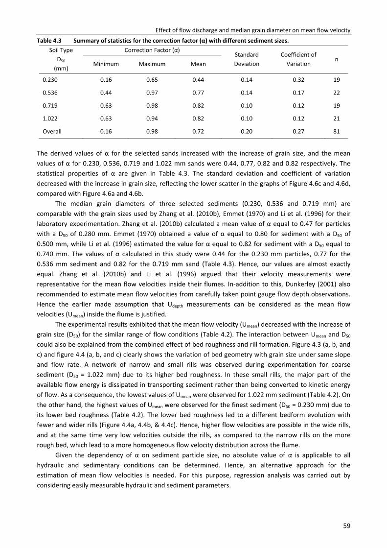
Effect of flow discharge and median grain diameter on mean flow velocity
59
Table 4.3 Summary of statistics for the correction factor (α) with different sediment sizes. Soil Type
D50 (mm)
Correction Factor (α)Standard Deviation
Coefficient of Variation
n Minimum Maximum Mean
0.230 0.16 0.65 0.44 0.14 0.32 19
0.536 0.44 0.97 0.77 0.14 0.17 22
0.719 0.63 0.98 0.82 0.10 0.12 19
1.022 0.63 0.94 0.82 0.10 0.12 21
Overall 0.16 0.98 0.72 0.20 0.27 81
The derived values of α for the selected sands increased with the increase of grain size, and the mean values of α for 0.230, 0.536, 0.719 and 1.022 mm sands were 0.44, 0.77, 0.82 and 0.82 respectively. The statistical properties of α are given in Table 4.3. The standard deviation and coefficient of variation decreased with the increase in grain size, reflecting the lower scatter in the graphs of Figure 4.6c and 4.6d, compared with Figure 4.6a and 4.6b.
The median grain diameters of three selected sediments (0.230, 0.536 and 0.719 mm) are comparable with the grain sizes used by Zhang et al. (2010b), Emmet (1970) and Li et al. (1996) for their laboratory experimentation. Zhang et al. (2010b) calculated a mean value of α equal to 0.47 for particles with a D50 of 0.280 mm. Emmet (1970) obtained a value of α equal to 0.80 for sediment with a D50 of 0.500 mm, while Li et al. (1996) estimated the value for α equal to 0.82 for sediment with a D50 equal to 0.740 mm. The values of α calculated in this study were 0.44 for the 0.230 mm particles, 0.77 for the 0.536 mm sediment and 0.82 for the 0.719 mm sand (Table 4.3). Hence, our values are almost exactly equal. Zhang et al. (2010b) and Li et al. (1996) argued that their velocity measurements were representative for the mean flow velocities inside their flumes. In-addition to this, Dunkerley (2001) also recommended to estimate mean flow velocities from carefully taken point gauge flow depth observations. Hence the earlier made assumption that Udepth measurements can be considered as the mean flow velocities (Umean) inside the flume is justified.
The experimental results exhibited that the mean flow velocity (Umean) decreased with the increase of grain size (D50) for the similar range of flow conditions (Table 4.2). The interaction between Umean and D50 could also be explained from the combined effect of bed roughness and rill formation. Figure 4.3 (a, b, and c) and figure 4.4 (a, b, and c) clearly shows the variation of bed geometry with grain size under same slope and flow rate. A network of narrow and small rills was observed during experimentation for coarse sediment (D50 = 1.022 mm) due to its higher bed roughness. In these small rills, the major part of the available flow energy is dissipated in transporting sediment rather than being converted to kinetic energy of flow. As a consequence, the lowest values of Umean were observed for 1.022 mm sediment (Table 4.2). On the other hand, the highest values of Umean were observed for the finest sediment (D50 = 0.230 mm) due to its lower bed roughness (Table 4.2). The lower bed roughness led to a different bedform evolution with fewer and wider rills (Figure 4.4a, 4.4b, & 4.4c). Hence, higher flow velocities are possible in the wide rills, and at the same time very low velocities outside the rills, as compared to the narrow rills on the more rough bed, which lead to a more homogeneous flow velocity distribution across the flume.
Given the dependency of α on sediment particle size, no absolute value of α is applicable to all hydraulic and sedimentary conditions can be determined. Hence, an alternative approach for the estimation of mean flow velocities is needed. For this purpose, regression analysis was carried out by considering easily measurable hydraulic and sediment parameters.
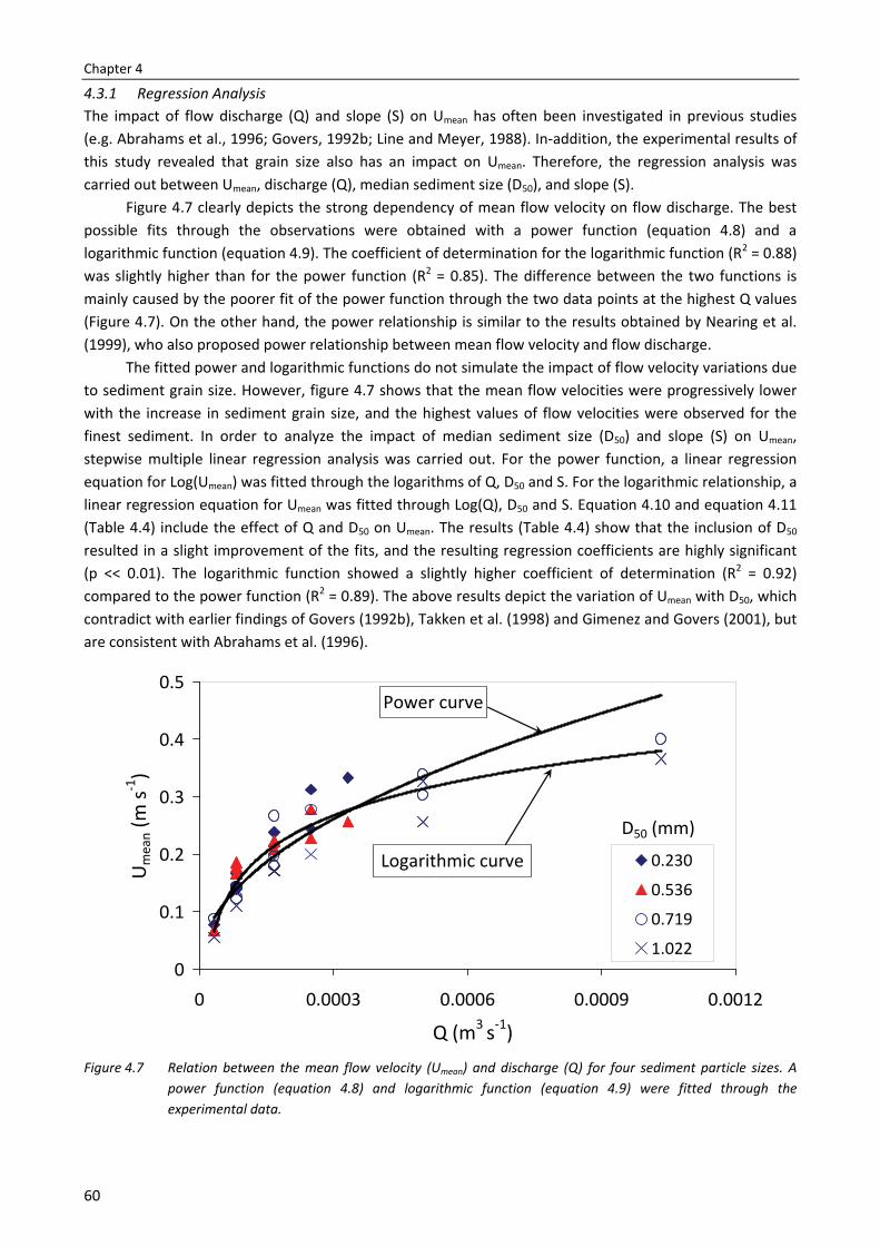
Chapter 4
60
4.3.1 Regression Analysis The impact of flow discharge (Q) and slope (S) on Umean has often been investigated in previous studies (e.g. Abrahams et al., 1996; Govers, 1992b; Line and Meyer, 1988). In-addition, the experimental results of this study revealed that grain size also has an impact on Umean. Therefore, the regression analysis was carried out between Umean, discharge (Q), median sediment size (D50), and slope (S).
Figure 4.7 clearly depicts the strong dependency of mean flow velocity on flow discharge. The best possible fits through the observations were obtained with a power function (equation 4.8) and a logarithmic function (equation 4.9). The coefficient of determination for the logarithmic function (R2 = 0.88) was slightly higher than for the power function (R2 = 0.85). The difference between the two functions is mainly caused by the poorer fit of the power function through the two data points at the highest Q values (Figure 4.7). On the other hand, the power relationship is similar to the results obtained by Nearing et al. (1999), who also proposed power relationship between mean flow velocity and flow discharge.
The fitted power and logarithmic functions do not simulate the impact of flow velocity variations due to sediment grain size. However, figure 4.7 shows that the mean flow velocities were progressively lower with the increase in sediment grain size, and the highest values of flow velocities were observed for the finest sediment. In order to analyze the impact of median sediment size (D50) and slope (S) on Umean, stepwise multiple linear regression analysis was carried out. For the power function, a linear regression equation for Log(Umean) was fitted through the logarithms of Q, D50 and S. For the logarithmic relationship, a linear regression equation for Umean was fitted through Log(Q), D50 and S. Equation 4.10 and equation 4.11 (Table 4.4) include the effect of Q and D50 on Umean. The results (Table 4.4) show that the inclusion of D50 resulted in a slight improvement of the fits, and the resulting regression coefficients are highly significant (p << 0.01). The logarithmic function showed a slightly higher coefficient of determination (R2 = 0.92) compared to the power function (R2 = 0.89). The above results depict the variation of Umean with D50, which contradict with earlier findings of Govers (1992b), Takken et al. (1998) and Gimenez and Govers (2001), but are consistent with Abrahams et al. (1996).
Figure 4.7 Relation between the mean flow velocity (Umean) and discharge (Q) for four sediment particle sizes. A
power function (equation 4.8) and logarithmic function (equation 4.9) were fitted through the experimental data.
0
0.1
0.2
0.3
0.4
0.5
0 0.0003 0.0006 0.0009 0.0012
Q (m3 s-1)
Um
ean (
m s-1
)
0.230
0.536
0.719
1.022
D50 (mm)
Power curve
Logarithmic curve
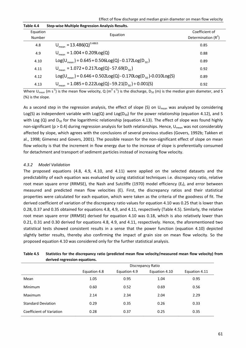
Effect of flow discharge and median grain diameter on mean flow velocity
61
Table 4.4 Step-wise Multiple Regression Analysis Results. Equation Number
Equation Coefficient of
Determination (R2)
4.8 0.4863mean (Q)13.486=U 0.85
4.9 Log(Q)0.209+1.004=Umean 0.88
4.10 )Log(D0.172Log(Q)0.506+0.645=)Log(U 50mean - 0.89
4.11 )(D57.69-Log(Q)0.217+1.072=U 50mean 0.92
4.12 )S(Log010.0-)Log(D0.170-Log(Q)0.502+0.646=)Log(U 50mean 0.89
4.13 )S(001.0)(D59.21Log(Q)0.222+1.085=U 50mean +- 0.92
Where Umean (m s-1) is the mean flow velocity, Q (m3 s-1) is the discharge, D50 (m) is the median grain diameter, and S (%) is the slope.
As a second step in the regression analysis, the effect of slope (S) on Umean was analyzed by considering Log(S) as independent variable with Log(Q) and Log(D50) for the power relationship (equation 4.12), and S with Log (Q) and D50 for the logarithmic relationship (equation 4.13). The effect of slope was found highly non-significant (p > 0.4) during regression analysis for both relationships. Hence, Umean was not considerably affected by slope, which agrees with the conclusions of several previous studies (Govers, 1992b; Takken et al., 1998; Gimenez and Govers, 2001). The possible reason for the non-significant effect of slope on mean flow velocity is that the increment in flow energy due to the increase of slope is preferentially consumed for detachment and transport of sediment particles instead of increasing flow velocity.
4.3.2 Model Validation The proposed equations (4.8, 4.9, 4.10, and 4.11) were applied on the selected datasets and the predictability of each equation was evaluated by using statistical techniques i.e. discrepancy ratio, relative root mean square error (RRMSE), the Nash and Sutcliffe (1970) model efficiency (Ef), and error between measured and predicted mean flow velocities (E). First, the discrepancy ratios and their statistical properties were calculated for each equation, which were taken as the criteria of the goodness of fit. The derived coefficient of variation of the discrepancy ratio values for equation 4.10 was 0.25 that is lower than 0.28, 0.37 and 0.35 obtained for equations 4.8, 4.9, and 4.11, respectively (Table 4.5). Similarly, the relative root mean square error (RRMSE) derived for equation 4.10 was 0.18, which is also relatively lower than 0.21, 0.31 and 0.30 derived for equations 4.8, 4.9, and 4.11, respectively. Hence, the aforementioned two statistical tests showed consistent results in a sense that the power function (equation 4.10) depicted slightly better results, thereby also confirming the impact of grain size on mean flow velocity. So the proposed equation 4.10 was considered only for the further statistical analysis.
Table 4.5 Statistics for the discrepancy ratio (predicted mean flow velocity/measured mean flow velocity) from
derived regression equations. Discrepancy Ratio
Equation 4.8 Equation 4.9 Equation 4.10 Equation 4.11
Mean 1.05 0.95 1.04 0.95
Minimum 0.60 0.52 0.69 0.56
Maximum 2.14 2.34 2.04 2.29
Standard Deviation 0.29 0.35 0.26 0.33
Coefficient of Variation 0.28 0.37 0.25 0.35
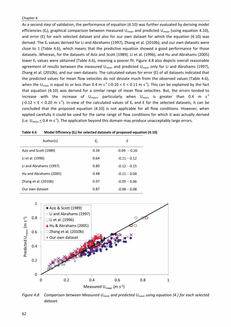
Chapter 4
62
As a second step of validation, the performance of equation (4.10) was further evaluated by deriving model efficiencies (Ef), graphical comparison between measured Umean and predicted Umean (using equation 4.10), and error (E) for each selected dataset and also for our own dataset for which the equation (4.10) was derived. The Ef values derived for Li and Abrahams (1997), Zhang et al. (2010b), and our own datasets were close to 1 (Table 4.6), which means that the predictive equation showed a good performance for those datasets. Whereas, for the datasets of Aziz and Scott (1989), Li et al. (1996), and Hu and Abrahams (2005) lower Ef values were obtained (Table 4.6), meaning a poorer fit. Figure 4.8 also depicts overall reasonable agreement of results between the measured Umean and predicted Umean only for Li and Abrahams (1997), Zhang et al. (2010b), and our own datasets. The calculated values for error (E) of all datasets indicated that the predicted values for mean flow velocites do not deviate much from the observed values (Table 4.6), when the Umean is equal to or less than 0.4 m s-1 (-0.10 < E < 0.11 m s-1). This can be explained by the fact that equation (4.10) was derived for a similar range of mean flow velocities. But, the errors tended to increase with the increase of Umean, particularly when Umean is greater than 0.4 m s-1 (-0.12 < E < 0.20 m s-1). In-view of the calculated values of Ef and E for the selected datasets, it can be concluded that the proposed equation (4.10) is not applicable for all flow conditions. However, when applied carefully it could be used for the same range of flow conditions for which it was actually derived (i.e. Umean < 0.4 m s-1). The application beyond this domain may produce unacceptably large errors.
Table 4.6 Model Efficiency (Ef) for selected datasets of proposed equation (4.10)
Author(s) Ef E
Aziz and Scott (1989) 0.34 -0.09 ∼ 0.20
Li et al. (1996) 0.64 -0.11 ∼ 0.12
Li and Abrahams (1997) 0.80 -0.12 ∼ 0.15
Hu and Abrahams (2005) 0.48 -0.11 ∼ 0.04
Zhang et al. (2010b) 0.97 -0.05 ∼ 0.06
Our own dataset 0.87 -0.08 ∼ 0.08
Figure 4.8 Comparison between Measured Umean and predicted Umean using equation (4.) for each selected
dataset.
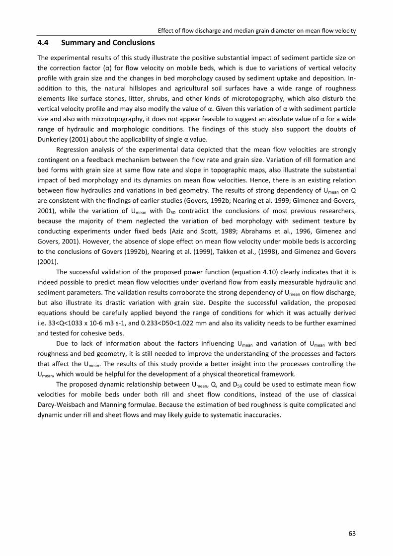
Effect of flow discharge and median grain diameter on mean flow velocity
63
4.4 Summary and Conclusions
The experimental results of this study illustrate the positive substantial impact of sediment particle size on the correction factor (α) for flow velocity on mobile beds, which is due to variations of vertical velocity profile with grain size and the changes in bed morphology caused by sediment uptake and deposition. In-addition to this, the natural hillslopes and agricultural soil surfaces have a wide range of roughness elements like surface stones, litter, shrubs, and other kinds of microtopography, which also disturb the vertical velocity profile and may also modify the value of α. Given this variation of α with sediment particle size and also with microtopography, it does not appear feasible to suggest an absolute value of α for a wide range of hydraulic and morphologic conditions. The findings of this study also support the doubts of Dunkerley (2001) about the applicability of single α value.
Regression analysis of the experimental data depicted that the mean flow velocities are strongly contingent on a feedback mechanism between the flow rate and grain size. Variation of rill formation and bed forms with grain size at same flow rate and slope in topographic maps, also illustrate the substantial impact of bed morphology and its dynamics on mean flow velocities. Hence, there is an existing relation between flow hydraulics and variations in bed geometry. The results of strong dependency of Umean on Q are consistent with the findings of earlier studies (Govers, 1992b; Nearing et al. 1999; Gimenez and Govers, 2001), while the variation of Umean with D50 contradict the conclusions of most previous researchers, because the majority of them neglected the variation of bed morphology with sediment texture by conducting experiments under fixed beds (Aziz and Scott, 1989; Abrahams et al., 1996, Gimenez and Govers, 2001). However, the absence of slope effect on mean flow velocity under mobile beds is according to the conclusions of Govers (1992b), Nearing et al. (1999), Takken et al., (1998), and Gimenez and Govers (2001).
The successful validation of the proposed power function (equation 4.10) clearly indicates that it is indeed possible to predict mean flow velocities under overland flow from easily measurable hydraulic and sediment parameters. The validation results corroborate the strong dependency of Umean on flow discharge, but also illustrate its drastic variation with grain size. Despite the successful validation, the proposed equations should be carefully applied beyond the range of conditions for which it was actually derived i.e. 33<Q<1033 x 10-6 m3 s-1, and 0.233<D50<1.022 mm and also its validity needs to be further examined and tested for cohesive beds.
Due to lack of information about the factors influencing Umean and variation of Umean with bed roughness and bed geometry, it is still needed to improve the understanding of the processes and factors that affect the Umean. The results of this study provide a better insight into the processes controlling the Umean, which would be helpful for the development of a physical theoretical framework.
The proposed dynamic relationship between Umean, Q, and D50 could be used to estimate mean flow velocities for mobile beds under both rill and sheet flow conditions, instead of the use of classical Darcy-Weisbach and Manning formulae. Because the estimation of bed roughness is quite complicated and dynamic under rill and sheet flows and may likely guide to systematic inaccuracies.

Chapter 5
Effect of hydraulic parameters on sediment transport capacity in overland flow over erodible beds
Ali M., Sterk G., Seeger M., Boersema M. and P. Peters Hydrology and Earth System Sciences Discussions 8: 6939–6965 (2011).

67
Effect of hydraulic parameters on sediment transport capacity in overland flow over erodible beds
Abstract
Sediment transport is an important component of the soil erosion process, which depends on several hydraulic parameters like unit discharge, mean flow velocity, and slope gradient. In most of the previous studies, the impact of these hydraulic parameters on transport capacity was studied for non-erodible bed conditions. Hence, this study aimed to examine the influence of unit discharge, mean flow velocity and slope gradient on sediment transport capacity for erodible beds and also to investigate the relationship between transport capacity and composite force predictors i.e. shear stress, stream power, unit stream power and effective stream power. In order to accomplish the objectives, experiments were carried out using four well sorted sands (0.230, 0.536, 0.719, 1.022 mm). Unit discharges ranging from 0.07 to 2.07 x 10⁻³ m2 s-1 were simulated inside the flume at four slopes (5.2, 8.7, 13.2 and 17.6%) to analyze their impact on sediment transport rate. The sediment transport rate measured at the bottom end of the flume by taking water and sediment samples was considered equal to sediment transport capacity, because the selected flume length of 3.0 m was found sufficient to reach the transport capacity. The experimental result reveals that the slope gradient has a stronger impact on transport capacity than unit discharge and mean flow velocity due to the fact that the tangential component of gravity force increases with slope gradient. Our results show that unit stream power is an optimal composite force predictor for estimating transport capacity. Stream power and effective stream power can also be successfully related to the transport capacity, however the relations are strongly dependent on grain size. Shear stress showed poor performance, because part of shear stress is dissipated by bed irregularities, bed form evolution and sediment detachment. An empirical transport capacity equation was derived, which illustrates that transport capacity can be predicted from median grain size, total discharge and slope gradient.
5.1 Introduction
Soil erosion has become a major global environmental problem (Lal, 1998). Several physically based soil erosion models have been developed to estimate sediment yield at the catchment scale (KINEROS2, Smith et al., 1995; LISEM, De Roo et al., 1996; EUROSEM; Morgan et al., 1998a,b; WEPP, Flanagan et al., 2001). Soil erosion is a combination of detachment and transport of sediment particles. An accurate estimation of these processes is the main objective of a physically based model. Most of the existing models estimate sediment detachment by using the concept of Foster and Meyer (1972). According to this concept, the detachment rate of flowing water is calculated as the difference between the sediment transport capacity and actual sediment load. Hence, sediment transport capacity plays a pivotal role in the physical description of soil erosion processes.
Sediment transport capacity is defined as the maximum sediment load that a particular discharge can transport at a certain slope (Merten et al., 2001). During the last three decades, several efforts have been made to analyze the influence of different hydraulic parameters on transport capacity, such as unit discharge, mean flow velocity, and slope gradient (Beasley and Huggins, 1982; Julien and Simons, 1985; Govers and Rauws, 1986; Finkner et al., 1989; Govers, 1990; Guy et al., 1990: Everaert, 1991; Govers, 1992a; Abrahams and Li, 1998; Jayawardena and Bhuiyan, 1999; Prosser and Rustomji, 2000; Abrahams et al., 2001; Zhang et al., 2009). The influence of these hydraulic parameters has mainly been studied using datasets obtained from flume experiments, which had non-erodible beds. For erodible bed experiments,
Chapter 5
68
previous researchers usually assumed that their selected flume length was adequate to reach the transport capacity (e.g. Govers, 1990; Everaert, 1991). But, qualitative and quantitative information about the spatial variation in sediment load is needed to verify this assumption.
The relationship between transport capacity and unit discharge has often been studied, and previous research has made it clear that this relationship is always dependent on slope (Beasley and Huggins, 1982; Julien and Simons, 1985; Govers and Rauws, 1986; Govers, 1990; Everaert, 1991; Jayawardena and Bhuiyan, 1999; Prosser and Rustomji, 2000; Lei et al., 2001; Zhang et al., 2009). However, the effect of unit discharge and slope on transport capacity varies from erodible to non-erodible bed conditions (Gover, 1990; Everaert, 1991; Zhang et al., 2009), probably due to the fact that, for the same hydraulic and sediment conditions the roughness of erodible beds is always higher than that of non-erodible beds (Hu and Abrahams, 2006). Govers (1990) and Everaert (1991) found, in different studies, that for erodible beds the effect of slope on transport capacity is higher than the effect of unit discharge. However, the non-erodible bed experiments of Zhang et al. (2009) revealed that transport capacity is more susceptible to unit discharge as compared to slope, contradicting the previously mentioned results. This raises questions about the applicability of information obtained from non-erodible beds for the development of sediment transport functions to be used in soil erosion models.
The influence of mean flow velocity on transport capacity has been studied mainly under non-erodible bed conditions (Guy et al., 1990; Abrahams and Li, 1998; Zhang et al., 2009; Zhang et al., 2010a,c). Guy et al. (1990) found that transport capacity increases as mean flow velocity increases, because mean flow velocity consistently increases with slope. Zhang et al. (2009) even reported a linear increase of transport capacity with increasing mean flow velocity for non-erodible beds. Again, contradicting results were found under erodible bed conditions (Govers, 1990; Nearing et al., 1997; Takken et al., 1998; Nearing et al., 1999; Gimenez and Govers, 2001), where the influence of slope on flow velocity was non-significant and, consequently, flow velocity had no clear influence on sediment transport capacity. As a result, it is clear that there is a need to comprehensively study the influence of different hydraulic parameters on sediment transport capacity.
Several scientists have used composite force predictors to estimate transport capacity of overland flow (Yang, 1972; Moore and Burch, 1986; Govers and Rauws; 1986; Lu et al., 1989; Govers, 1990; Everaert, 1991; Govers, 1992a; Jayawardena and Bhuiyan, 1999; Prosser and Rustomji, 2000; Abrahams et al., 2001; Zhang et al., 2009). Hydraulic variables were combined in different ways to form composite force predictors for the estimation of transport capacity i.e. shear stress, stream power, unit stream power, and effective stream power (Duboys, 1879; Bagnold, 1966; Yang, 1972; Govers, 1990). But widely varying results were obtained, because the performance of composite force predictors were tested under different ranges of morphologic conditions. Govers and Rauws (1986) concluded that shear stress is not a good predictor for estimating transport capacity under erodible bed conditions, because an important component of the shear stress (i.e. form shear stress) may not be actively used for sediment transport, but could be preferentially consumed on sediment detachment and bed form evolution. Therefore, they suggested the use of grain shear stress (the part of shear stress consumed on individual grains) and unit stream power concepts to predict transport capacity on erodible beds. However, later results from Govers (1990) contradict the recommendations of Govers and Rauws (1986), showing that shear stress can be used to estimate transport capacity under erodible beds. In addition, the experimental results of Zhang et al. (2009) also depicted that transport capacity was well predicted by shear stress for non-erodible bed conditions.
The influence of unit discharge and mean flow velocity on transport capacity under erodible bed conditions is still ambiguous, and needs to be further examined, in order to get a better understanding of the processes involved in sediment transport by overland flow. In addition, the selection of a suitable composite predictor for the estimation of transport capacity is also still uncertain. Therefore, the objectives
Effect of hydraulic parameters on sediment transport capacity over erodible beds
69
of this research were (i) to study the effect of unit discharge, mean flow velocity and slope gradient on sediment transport capacity and how these relations vary in the presence and absence of bed irregularities, and (ii) to evaluate the potential of different composite force predictors for the estimation of transport capacity under overland flow conditions. Fundamental for addressing these objectives is knowing if the selected experimental setup is sufficient for reaching the transport capacity. To tackle these objectives, an experiment on erodible beds was designed with variable slopes, discharges and grain sizes.
5.2 Materials and methods
For this study, a 3.0 m long and 0.5 m wide rectangular flume with a wooden floor and one sided plexiglass wall was constructed. The experimental set-up was similar to the one described by Ali et al. (2011b). In order to abridge the edge effects, a piece of wood (length = 0.20, width = 0.50, height = 0.04 m, “stopper”) was fixed at the upper end of the flume and a second stopper (length = 0.10, width = 0.50, height = 0.04 m) was fixed at the lower end (Figure 5.1). The upper stopper also allows the water to enter into the test section from the head tank avoiding erosion and causing uniform spreading of the applied discharge across the flume width. The length of the lower stopper (i.e. 0.10 m) was selected to allow passing of the water and sediment mixture without causing any serious deposition. Tap water was used to conduct the experiments, which entered into the flume from a head tank. The rate of flow into the head tank was controlled by a valve and measured with a calibrated flow-meter at the inlet pipe. The flow-meter was connected to a data-logger and computer for continuous monitoring of the inflow rate. The applied unit discharge rates ranged from 0.07 to 2.07 x 10⁻³ m2 s-1.
In order to study the variation of sediment transport capacity with grain size, four well sorted non-cohesive medium to very coarse sands with median grain size (D50) equal to 0.233, 0.536, 0.719, and 1.022 mm and their bulk density equal to 1600 kg m-3 were used. Prior to each experiment, the test section was filled with a 0.04 m thick layer of sediment and saturated with water. The contact area between the upper stopper and sand layer was covered with a piece of artificial grass carpet, in order to dissipate the flow energy of the inflowing water. However, sudden high rates of erosion could not be fully prevented. For the experiments, the flume bed was adjusted to four slope gradients (5.2, 8.7, 13.2 and 17.6%), to analyze the impact of slope on sediment transport capacity. Before each experiment, test runs were carried out to adjust the duration of the inflow for each combination of applied unit discharge, slope gradient and sediment type. As a result of these test runs, the time to conduct experiments ranged between 5 and 30 minutes. Each experimental run was repeated once to ensure the results.
As flow depths are usually hard to assess under overland flow conditions on a changing bed due to the unsteadiness of the water and bed surface, two point gauges with an accuracy of 0.1 mm were hung on a wooden frame above the lower stopper of the flume, directly downstream of the sand bed. The mean flow depth was calculated by taking the average of the measurements taken from both gauges.
Mean flow velocity is difficult to measure under interrill and rill erosion due to spatial variation of bed geometry and limited flow depth (Jayawardena and Bhuiyan, 1999). The conversion of surface flow velocity measurements into mean flow velocity has also become a challenge, because of the selection of a suitable correction factor (Dunkerley, 2001). Hence in this study, mean flow velocities were estimated using the equation derived by Ali et al. (2011b) for the same flume.
)Log(D0.172Log(Q)0.506+0.645=Log(U) 50− [5.1]
Where U (m s-1) is the mean flow velocity, Q (m3 s-1) is the total discharge, and D50 (m) is the median grain diameter of the bed material.
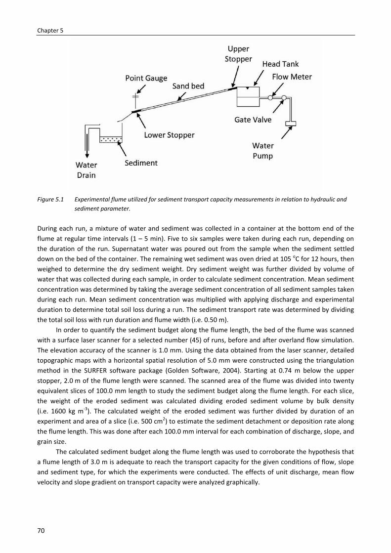
Chapter 5
70
Figure 5.1 Experimental flume utilized for sediment transport capacity measurements in relation to hydraulic and sediment parameter. During each run, a mixture of water and sediment was collected in a container at the bottom end of the flume at regular time intervals (1 – 5 min). Five to six samples were taken during each run, depending on the duration of the run. Supernatant water was poured out from the sample when the sediment settled down on the bed of the container. The remaining wet sediment was oven dried at 105 oC for 12 hours, then weighed to determine the dry sediment weight. Dry sediment weight was further divided by volume of water that was collected during each sample, in order to calculate sediment concentration. Mean sediment concentration was determined by taking the average sediment concentration of all sediment samples taken during each run. Mean sediment concentration was multiplied with applying discharge and experimental duration to determine total soil loss during a run. The sediment transport rate was determined by dividing the total soil loss with run duration and flume width (i.e. 0.50 m).
In order to quantify the sediment budget along the flume length, the bed of the flume was scanned with a surface laser scanner for a selected number (45) of runs, before and after overland flow simulation. The elevation accuracy of the scanner is 1.0 mm. Using the data obtained from the laser scanner, detailed topographic maps with a horizontal spatial resolution of 5.0 mm were constructed using the triangulation method in the SURFER software package (Golden Software, 2004). Starting at 0.74 m below the upper stopper, 2.0 m of the flume length were scanned. The scanned area of the flume was divided into twenty equivalent slices of 100.0 mm length to study the sediment budget along the flume length. For each slice, the weight of the eroded sediment was calculated dividing eroded sediment volume by bulk density (i.e. 1600 kg m-3). The calculated weight of the eroded sediment was further divided by duration of an experiment and area of a slice (i.e. 500 cm2) to estimate the sediment detachment or deposition rate along the flume length. This was done after each 100.0 mm interval for each combination of discharge, slope, and grain size.
The calculated sediment budget along the flume length was used to corroborate the hypothesis that a flume length of 3.0 m is adequate to reach the transport capacity for the given conditions of flow, slope and sediment type, for which the experiments were conducted. The effects of unit discharge, mean flow velocity and slope gradient on transport capacity were analyzed graphically.
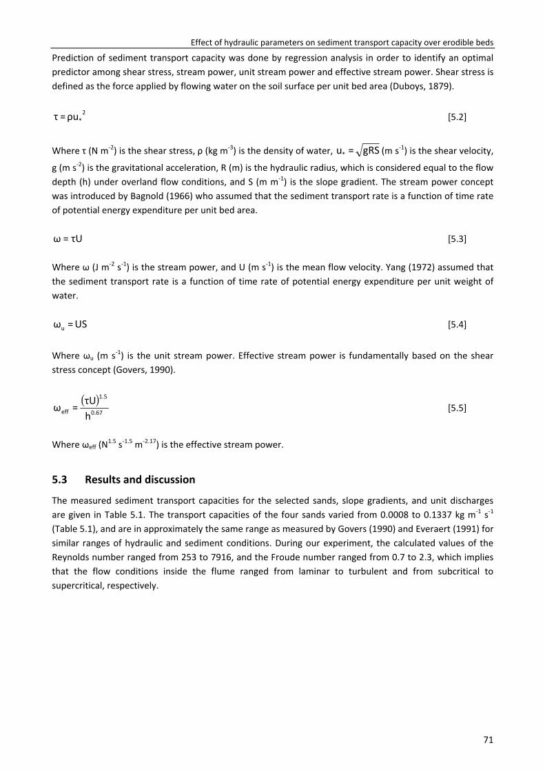
Effect of hydraulic parameters on sediment transport capacity over erodible beds
71
Prediction of sediment transport capacity was done by regression analysis in order to identify an optimal predictor among shear stress, stream power, unit stream power and effective stream power. Shear stress is defined as the force applied by flowing water on the soil surface per unit bed area (Duboys, 1879).
2*ρu=τ [5.2]
Where τ (N m-2) is the shear stress, ρ (kg m-3) is the density of water, gRS=u* (m s-1) is the shear velocity,
g (m s-2) is the gravitational acceleration, R (m) is the hydraulic radius, which is considered equal to the flow depth (h) under overland flow conditions, and S (m m-1) is the slope gradient. The stream power concept was introduced by Bagnold (1966) who assumed that the sediment transport rate is a function of time rate of potential energy expenditure per unit bed area.
τU=ω [5.3] Where ω (J m-2 s-1) is the stream power, and U (m s-1) is the mean flow velocity. Yang (1972) assumed that the sediment transport rate is a function of time rate of potential energy expenditure per unit weight of water.
US=ωu [5.4]
Where ωu (m s-1) is the unit stream power. Effective stream power is fundamentally based on the shear stress concept (Govers, 1990).
( )0.67
1.5
eff hτU=ω [5.5]
Where ωeff (N1.5 s-1.5 m-2.17) is the effective stream power.
5.3 Results and discussion
The measured sediment transport capacities for the selected sands, slope gradients, and unit discharges are given in Table 5.1. The transport capacities of the four sands varied from 0.0008 to 0.1337 kg m-1 s-1 (Table 5.1), and are in approximately the same range as measured by Govers (1990) and Everaert (1991) for similar ranges of hydraulic and sediment conditions. During our experiment, the calculated values of the Reynolds number ranged from 253 to 7916, and the Froude number ranged from 0.7 to 2.3, which implies that the flow conditions inside the flume ranged from laminar to turbulent and from subcritical to supercritical, respectively.
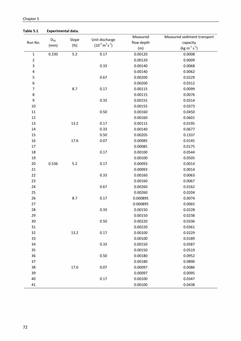
Chapter 5
72
Table 5.1 Experimental data.
Run No. D50
(mm) Slope
(%) Unit discharge
(10-3 m2 s-1)
Measuredflow depth
(m)
Measured sediment transport capacity
(kg m-1 s-1) 1 0.230 5.2 0.17 0.00120 0.0008 2 0.00120 0.0009 3 0.33 0.00140 0.0068 4 0.00140 0.0062 5 0.67 0.00200 0.0229 6 0.00200 0.0312 7 8.7 0.17 0.00115 0.0099 8 0.00115 0.0076 9 0.33 0.00155 0.0314
10 0.00155 0.0373 11 0.50 0.00160 0.0450 12 0.00160 0.0601 13 13.2 0.17 0.00115 0.0195 14 0.33 0.00140 0.0677 15 0.50 0.00205 0.1337 16 17.6 0.07 0.00085 0.0145 17 0.00085 0.0175 18 0.17 0.00100 0.0544 19 0.00100 0.0505 20 0.536 5.2 0.17 0.00093 0.0014 21 0.00093 0.0014 22 0.33 0.00160 0.0063 23 0.00160 0.0067 24 0.67 0.00260 0.0162 25 0.00260 0.0204 26 8.7 0.17 0.000895 0.0074 27 0.000895 0.0065 28 0.33 0.00150 0.0228 29 0.00150 0.0238 30 0.50 0.00220 0.0336 31 0.00220 0.0361 32 13.2 0.17 0.00100 0.0229 33 0.00100 0.0189 34 0.33 0.00150 0.0587 35 0.00150 0.0519 36 0.50 0.00180 0.0952 37 0.00180 0.0890 38 17.6 0.07 0.00097 0.0086 39 0.00097 0.0095 40 0.17 0.00100 0.0347 41 0.00100 0.0438
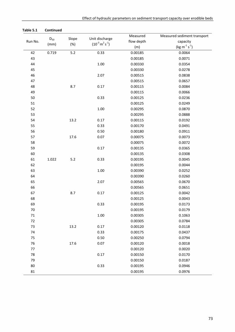
Effect of hydraulic parameters on sediment transport capacity over erodible beds
73
Table 5.1 Continued
Run No. D50
(mm) Slope
(%) Unit discharge
(10-3 m2 s-1)
Measuredflow depth
(m)
Measured sediment transport capacity
(kg m-1 s-1) 42 0.719 5.2 0.33 0.00185 0.0064 43 0.00185 0.0071 44 1.00 0.00330 0.0354 45 0.00330 0.0278 46 2.07 0.00515 0.0838 47 0.00515 0.0657 48 8.7 0.17 0.00115 0.0084 49 0.00115 0.0066 50 0.33 0.00125 0.0236 51 0.00125 0.0249 52 1.00 0.00295 0.0870 53 0.00295 0.0888 54 13.2 0.17 0.00115 0.0192 55 0.33 0.00170 0.0491 56 0.50 0.00180 0.0911 57 17.6 0.07 0.00075 0.0073 58 0.00075 0.0072 59 0.17 0.00135 0.0365 60 0.00135 0.0308 61 1.022 5.2 0.33 0.00195 0.0045 62 0.00195 0.0044 63 1.00 0.00390 0.0252 64 0.00390 0.0260 65 2.07 0.00565 0.0670 66 0.00565 0.0651 67 8.7 0.17 0.00125 0.0042 68 0.00125 0.0043 69 0.33 0.00195 0.0173 70 0.00195 0.0179 71 1.00 0.00305 0.1063 72 0.00305 0.0784 73 13.2 0.17 0.00120 0.0118 74 0.33 0.00175 0.0437 75 0.50 0.00250 0.0794 76 17.6 0.07 0.00120 0.0018 77 0.00120 0.0020 78 0.17 0.00150 0.0170 79 0.00150 0.0187 80 0.33 0.00195 0.0946 81 0.00195 0.0976
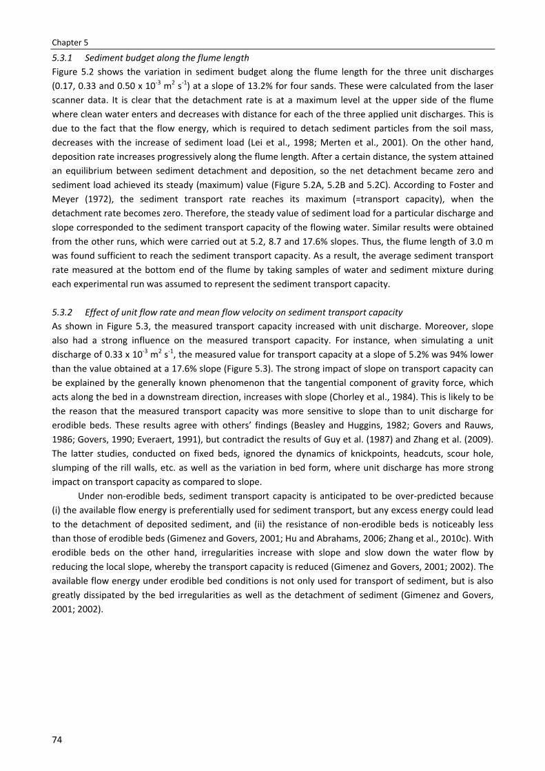
Chapter 5
74
5.3.1 Sediment budget along the flume length Figure 5.2 shows the variation in sediment budget along the flume length for the three unit discharges (0.17, 0.33 and 0.50 x 10⁻³ m2 s-1) at a slope of 13.2% for four sands. These were calculated from the laser scanner data. It is clear that the detachment rate is at a maximum level at the upper side of the flume where clean water enters and decreases with distance for each of the three applied unit discharges. This is due to the fact that the flow energy, which is required to detach sediment particles from the soil mass, decreases with the increase of sediment load (Lei et al., 1998; Merten et al., 2001). On the other hand, deposition rate increases progressively along the flume length. After a certain distance, the system attained an equilibrium between sediment detachment and deposition, so the net detachment became zero and sediment load achieved its steady (maximum) value (Figure 5.2A, 5.2B and 5.2C). According to Foster and Meyer (1972), the sediment transport rate reaches its maximum (=transport capacity), when the detachment rate becomes zero. Therefore, the steady value of sediment load for a particular discharge and slope corresponded to the sediment transport capacity of the flowing water. Similar results were obtained from the other runs, which were carried out at 5.2, 8.7 and 17.6% slopes. Thus, the flume length of 3.0 m was found sufficient to reach the sediment transport capacity. As a result, the average sediment transport rate measured at the bottom end of the flume by taking samples of water and sediment mixture during each experimental run was assumed to represent the sediment transport capacity.
5.3.2 Effect of unit flow rate and mean flow velocity on sediment transport capacity As shown in Figure 5.3, the measured transport capacity increased with unit discharge. Moreover, slope also had a strong influence on the measured transport capacity. For instance, when simulating a unit discharge of 0.33 x 10⁻³ m2 s-1, the measured value for transport capacity at a slope of 5.2% was 94% lower than the value obtained at a 17.6% slope (Figure 5.3). The strong impact of slope on transport capacity can be explained by the generally known phenomenon that the tangential component of gravity force, which acts along the bed in a downstream direction, increases with slope (Chorley et al., 1984). This is likely to be the reason that the measured transport capacity was more sensitive to slope than to unit discharge for erodible beds. These results agree with others’ findings (Beasley and Huggins, 1982; Govers and Rauws, 1986; Govers, 1990; Everaert, 1991), but contradict the results of Guy et al. (1987) and Zhang et al. (2009). The latter studies, conducted on fixed beds, ignored the dynamics of knickpoints, headcuts, scour hole, slumping of the rill walls, etc. as well as the variation in bed form, where unit discharge has more strong impact on transport capacity as compared to slope.
Under non-erodible beds, sediment transport capacity is anticipated to be over-predicted because (i) the available flow energy is preferentially used for sediment transport, but any excess energy could lead to the detachment of deposited sediment, and (ii) the resistance of non-erodible beds is noticeably less than those of erodible beds (Gimenez and Govers, 2001; Hu and Abrahams, 2006; Zhang et al., 2010c). With erodible beds on the other hand, irregularities increase with slope and slow down the water flow by reducing the local slope, whereby the transport capacity is reduced (Gimenez and Govers, 2001; 2002). The available flow energy under erodible bed conditions is not only used for transport of sediment, but is also greatly dissipated by the bed irregularities as well as the detachment of sediment (Gimenez and Govers, 2001; 2002).
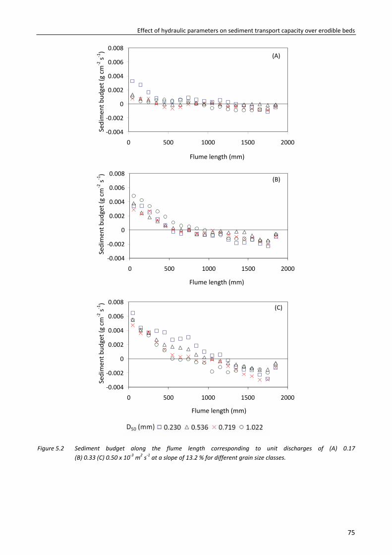
Effect of hydraulic parameters on sediment transport capacity over erodible beds
75
Figure 5.2 Sediment budget along the flume length corresponding to unit discharges of (A) 0.17 (B) 0.33 (C) 0.50 x 10⁻³ m2 s-1 at a slope of 13.2 % for different grain size classes.
-0.004
-0.002
0
0.002
0.004
0.006
0.008
0 500 1000 1500 2000
Flume length (mm)
Sedi
men
t bud
get (
g cm
-2 s-1
)
(A)
-0.004
-0.002
0
0.002
0.004
0.006
0.008
0 500 1000 1500 2000
Flume length (mm)
Sedi
men
t bud
get (
g cm
-2 s-1
)
(B)
-0.004
-0.002
0
0.002
0.004
0.006
0.008
0 500 1000 1500 2000
Flume length (mm)
Sedi
men
t bud
get (
g cm
-2 s-1
)
(C)
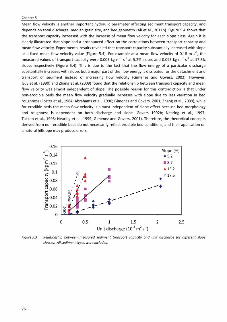
Chapter 5
76
Mean flow velocity is another important hydraulic parameter affecting sediment transport capacity, and depends on total discharge, median grain size, and bed geometry (Ali et al., 2011b). Figure 5.4 shows that the transport capacity increased with the increase of mean flow velocity for each slope class. Again it is clearly illustrated that slope had a pronounced effect on the correlations between transport capacity and mean flow velocity. Experimental results revealed that transport capacity substantially increased with slope at a fixed mean flow velocity value (Figure 5.4). For example at a mean flow velocity of 0.18 m s-1, the measured values of transport capacity were 0.003 kg m-1 s-1 at 5.2% slope, and 0.095 kg m-1 s-1 at 17.6% slope, respectively (Figure 5.4). This is due to the fact that the flow energy of a particular discharge substantially increases with slope, but a major part of the flow energy is dissipated for the detachment and transport of sediment instead of increasing flow velocity (Gimenez and Govers, 2002). However, Guy et al. (1990) and Zhang et al. (2009) found that the relationship between transport capacity and mean flow velocity was almost independent of slope. The possible reason for this contradiction is that under non-erodible beds the mean flow velocity gradually increases with slope due to less variation in bed roughness (Foster et al., 1984; Abrahams et al., 1996; Gimenez and Govers, 2001; Zhang et al., 2009), while for erodible beds the mean flow velocity is almost independent of slope effect because bed morphology and roughness is dependent on both discharge and slope (Govers 1992b; Nearing et al., 1997; Takken et al., 1998; Nearing et al., 1999; Gimenez and Govers, 2001). Therefore, the theoretical concepts derived from non-erodible beds do not necessarily reflect erodible bed conditions, and their application on a natural hillslope may produce errors.
Figure 5.3 Relationship between measured sediment transport capacity and unit discharge for different slope
classes. All sediment types were included.
0
0.02
0.04
0.06
0.08
0.1
0.12
0.14
0.16
0 0.5 1 1.5 2 2.5Unit discharge (10-3 m2 s-1)
Tran
spor
t cap
acity
(kg
m-1
s-1)
5.28.713.217.6
Slope (%)
Effect of hydraulic parameters on sediment transport capacity over erodible beds
77
Figure 5.4 Relationship between measured sediment transport capacity and mean flow velocity for different slope
classes. All sediment types were included.
5.3.3 Prediction of sediment transport capacity In previous studies composite force predictors have often been correlated with sediment transport capacity and most of the time it has been found that the relationship between transport capacity and a composite predictor can vary with grain size (Govers and Rauws, 1986; Govers, 1990; Everaert, 1991; Abrahams and Li, 1998; Ferro, 1998; Jayawardena and Bhuiyan, 1999; Zhang et al., 2009). Because in this study four types of sand were used to conduct the experiments, it is expected that grain size also significantly affects the relationships between transport capacity and composite force predictors.
Sediment transport capacity was modelled as a power function of composite force predictors i.e. shear stress, stream power, unit stream power, and effective stream power by using the entire dataset of the four different grain sizes (Figure 5.5). The best agreement with transport capacity was obtained using unit stream power (Figure 5.5c). However, when a multiple linear regression analysis was used to estimate transport capacity as a function of unit stream power and grain size, it was not significantly affected by grain size (p=0.197). The non-significant effect of grain size on the relationship between transport capacity and unit stream power was somewhat surprising, because grain size has been seen to have considerable effect on mean flow velocity (Ali et al., 2011b). These results do agree with the findings of previous researchers (Govers and Rauws, 1986; Moore and Burch, 1986; Govers, 1990) in such a way that the unit stream power theory showed greatest potential for estimating transport capacity of overland flow under erodible beds. But they contradict earlier findings in the sense that the exponent of unit stream power was independent of grain size.
The regression analysis between transport capacity and unit stream power produced the following relationship.
2.89uc 2326.6ω=T R2 = 0.87 [5.6]
Where Tc (kg m-1 s-1) is the sediment transport capacity and ωu (m s-1) is the unit stream power.
The performance of shear stress was poor as compared to other composite predictors (Figure 5.5a). The possible reason for its poor performance is that the shear stress required to attain a certain value of
0
0.02
0.04
0.06
0.08
0.1
0.12
0.14
0.16
0 0.1 0.2 0.3 0.4 0.5Mean flow velocity (m s-1)
Tran
spor
t cap
acity
(kg
m-1
s-1)
5.28.713.217.6
Slope (%)
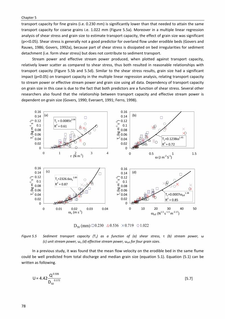
Chapter 5
78
transport capacity for fine grains (i.e. 0.230 mm) is significantly lower than that needed to attain the same transport capacity for coarse grains i.e. 1.022 mm (Figure 5.5a). Moreover in a multiple linear regression analysis of shear stress and grain size to estimate transport capacity, the effect of grain size was significant (p<<0.05). Shear stress is generally not a good predictor for overland flow under erodible beds (Govers and Rauws, 1986; Govers, 1992a), because part of shear stress is dissipated on bed irregularities for sediment detachment (i.e. form shear stress) but does not contribute to sediment transport.
Stream power and effective stream power produced, when plotted against transport capacity, relatively lower scatter as compared to shear stress, thus both resulted in reasonable relationships with transport capacity (Figure 5.5b and 5.5d). Similar to the shear stress results, grain size had a significant impact (p<0.05) on transport capacity in the multiple linear regression analysis, relating transport capacity to stream power or effective stream power and grain size using all data. Dependency of transport capacity on grain size in this case is due to the fact that both predictors are a function of shear stress. Several other researchers also found that the relationship between transport capacity and effective stream power is dependent on grain size (Govers, 1990; Everaert, 1991; Ferro, 1998).
Figure 5.5 Sediment transport capacity (Tc) as a function of (a) shear stress, τ (b) stream power, ω (c) unit stream power, ωu (d) effective stream power, ωeff for four grain sizes.
In a previous study, it was found that the mean flow velocity on the erodible bed in the same flume could be well predicted from total discharge and median grain size (equation 5.1). Equation (5.1) can be written as following.
172.050
0.506
DQ4.42=U [5.7]
Tc = 0.0085τ2.06
R2 = 0.61
00.020.040.060.08
0.10.120.140.16
0 1 2 3 4 τ (N m-2)
T c (k
g m
-1 s-1
)
(a)
00.020.040.060.08
0.10.120.140.16
0 0.5 1 1.5ω (J m-2 S-1)
T c (k
g m
-1 s-1
)
Tc=0.1238ω1.45
R2 = 0.72
(b)
Tc=2326.6ωυ2.89
R2 = 0.87
00.020.040.060.08
0.10.120.140.16
0 0.01 0.02 0.03 0.04ωu (m s-1)
T c (k
g m
-1 s-1
)
(c)
00.020.040.060.08
0.10.120.140.16
0 10 20 30 40 50ωeff (N
1.5 s-1.5 m-2.17)
T c (k
g m
-1 s-1
)
Tc=0.0007ωeff1.38
R2 = 0.85
(d)
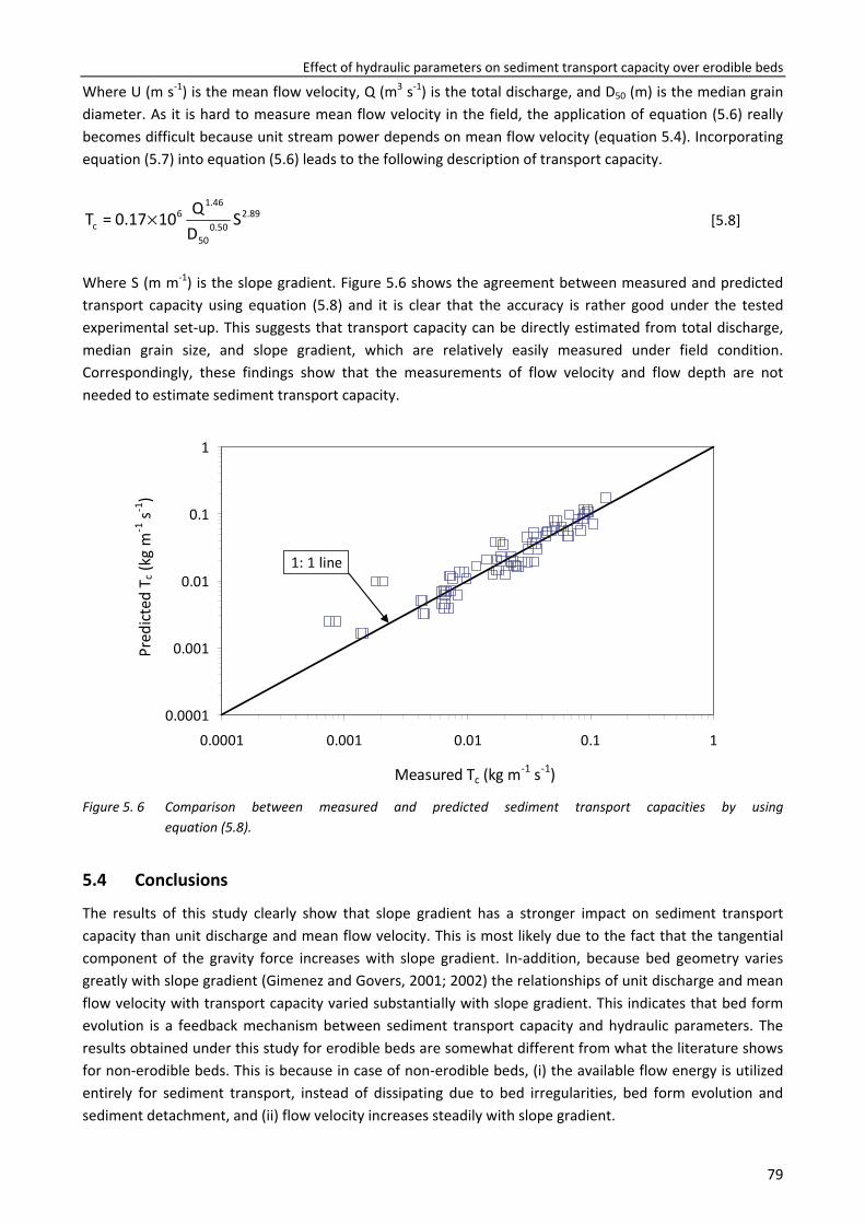
Effect of hydraulic parameters on sediment transport capacity over erodible beds
79
Where U (m s-1) is the mean flow velocity, Q (m3 s-1) is the total discharge, and D50 (m) is the median grain diameter. As it is hard to measure mean flow velocity in the field, the application of equation (5.6) really becomes difficult because unit stream power depends on mean flow velocity (equation 5.4). Incorporating equation (5.7) into equation (5.6) leads to the following description of transport capacity.
2.8950.0
50
1.466
c SDQ100.17=T × [5.8]
Where S (m m-1) is the slope gradient. Figure 5.6 shows the agreement between measured and predicted transport capacity using equation (5.8) and it is clear that the accuracy is rather good under the tested experimental set-up. This suggests that transport capacity can be directly estimated from total discharge, median grain size, and slope gradient, which are relatively easily measured under field condition. Correspondingly, these findings show that the measurements of flow velocity and flow depth are not needed to estimate sediment transport capacity.
Figure 5. 6 Comparison between measured and predicted sediment transport capacities by using
equation (5.8).
5.4 Conclusions
The results of this study clearly show that slope gradient has a stronger impact on sediment transport capacity than unit discharge and mean flow velocity. This is most likely due to the fact that the tangential component of the gravity force increases with slope gradient. In-addition, because bed geometry varies greatly with slope gradient (Gimenez and Govers, 2001; 2002) the relationships of unit discharge and mean flow velocity with transport capacity varied substantially with slope gradient. This indicates that bed form evolution is a feedback mechanism between sediment transport capacity and hydraulic parameters. The results obtained under this study for erodible beds are somewhat different from what the literature shows for non-erodible beds. This is because in case of non-erodible beds, (i) the available flow energy is utilized entirely for sediment transport, instead of dissipating due to bed irregularities, bed form evolution and sediment detachment, and (ii) flow velocity increases steadily with slope gradient.
0.0001
0.001
0.01
0.1
1
0.0001 0.001 0.01 0.1 1
Measured Tc (kg m-1 s-1)
Pred
icted
Tc (
kg m
-1 s-1
)
1: 1 line
Chapter 5
80
The experimental results showed that sediment transport capacity is well related to the selected composite force predictors, except shear stress. Unit stream power was the best performing composite predictor for estimation of transport capacity for shallow flows. A weaker relation was obtained between transport capacity and shear stress (R2 = 0.61), since part of shear stress is used to detach sediment particles from soil mass i.e. form shear stress. Despite the fact that stream power and effective stream power are functions of shear stress, both exhibited good potential for prediction of transport capacity, although the exponents of their relationships were found to be dependent on grain size. Among the selected composite predictors, unit stream power is preferred over other composite predictors, because (i) grain size has a non-significant effect on the relation between transport capacity and unit stream power, and (ii) mean flow velocity can be easily predicted from total discharge and median grain size (Ali et al., 2011b).
Overall, these results are entirely different from the results obtained from experiments with non-erodible beds, because both grain shear stress and form shear stress are utilized for sediment transport in the case of non-erodible beds (Zhang et al., 2009). The derived unit stream power based equation (equation 5.8) shows promise for use in physically based soil erosion models to more precisely estimate sediment transport capacity. More precise estimation of transport capacity is important in the ongoing challenge to better predict and manage soil erosion. Nonetheless, the equation suggested from this study was derived for non-cohesive narrowly graded sands, thus its validity needs to be further evaluated for cohesive soils.
Chapter 6
A unit stream power based sediment transport function for overland flow
Ali M., Seeger M., Sterk G. and D. Moore Catena (In review)

83
A unit stream power based sediment transport function for overland flow
Abstract
Erosion is a serious global problem requiring effective modeling for accurate assessment of erosion rates and sensitive areas. The outcome of soil erosion models depends strongly on the estimation of sediment transport capacity. In most of the existing spatially distributed soil erosion models, sediment transport capacity of overland flow is normally estimated using stream flow transport capacity functions. The applicability of stream flow functions to overland flow conditions is questionable because hydraulic conditions like flow depth and flow discharge under overland flow are substantially different from stream flow conditions. Hence, the main objectives of this study are to check the suitability of five existing well known and widely used transport capacity functions for use under overland flow conditions, and also to derive a new function by dimensional analysis to quantify transport capacity for overland flow. To accomplish the objectives, flume experiments were carried out using four different sands (0.230, 0.536, 0.719, and 1.022 mm). The unit discharges used for experimentation ranged from 0.07 to 2.07 x 10⁻³ m2 s-1 and slopes ranged from 5.2 to 17.6%. In this study, none of the results with the existing functions were in good agreement with measured results over the whole range of conditions, especially at low flow intensities. The percentage of observations in which the discrepancy ratio ranged between 0.5 and 2.0 were: 65% (Yalin), 74% (Low), 54% (Modified Engelund and Hansen), 57% (Govers), and 25% (Abrahams). The results showed that the selected functions reasonably estimate transport capacities only under those ranges of conditions for which they were formulated. Although the excess shear stress concept based function (i.e. Low’s function) produced excellent results, but the results varied substantially with grain size. In contrast, the unit stream power concept based Govers function exhibited quite similar results for all the selected sands. Based on the unit stream power concept, a new function for low flow intensities was derived by dimensional analysis using the experimental results. The newly derived function was calibrated using the flume experiment results, but validation is still needed for cohesive soils.
6.1 Introduction
Soil erosion is one of the world’s biggest environmental problems with both on-site and off-site effects in an agricultural watershed (Vigiak et al., 2005). Several spatially distributed soil erosion models are being widely used to assess the rate of erosion at catchment scale, and also to discover the areas in a catchment which are more susceptible to erosion (KINEROS2, Smith et al., 1995; LISEM, De Roo et al., 1996; EUROSEM, Morgan et al., 1998a; b; WEPP, Flanagan et al., 2001). The precise estimation of sediment transport capacity plays a vital role in the outcome of each soil erosion model because both the rate of sediment detachment and deposition depend strongly on it (Foster and Meyer, 1972). Sediment transport capacity is actually a maximum amount of a specific sediment type which can be transported at a certain discharge rate and slope (Merten et al., 2001). During the last three decades, a number of efforts have been made to understand the processes entailed in sediment transport and also to derive a transport capacity function (Julien and Simons, 1985; Govers and Rauws, 1986; Govers, 1990; Everaert, 1991; Govers, 1992a; Jayawardena and Bhuiyan, 1999; Prosser and Rustomji, 2000; Abrahams et al., 2001; Zhang et al., 2009; Ali et al., 2011a).
Many transport capacity functions have been derived for stream flow conditions (e.g. Yalin, 1963; Engelund and Hansen, 1967; Smart, 1984; Low, 1989). However the application of stream flow functions to
Chapter 6
84
overland flow conditions is questionable because the hydraulic conditions in overland flow are entirely different from the conditions in stream flow. For example, flow discharge and slope gradient under overland flow conditions are considerably different than under stream flow conditions (Hessel and Jetten, 2007). In view of the differences between stream flow and overland flow conditions, few researchers have derived empirical functions by regression analysis of their experimental results to quantify the transport capacity for overland flow (Govers and Rauws, 1986; Govers, 1990; Everaert, 1991; Govers, 1992a; Smith et al., 1995). Only Abrahams et al. (2001) developed a transport capacity function by dimensional analysis for overland flow conditions using a limited range of flume experimental results.
Since the 1980’s, several researchers evaluated the performance of many transport capacity functions under different ranges of hydraulic and sediment conditions and reached somewhat different conclusions (Alonso et al., 1981; Low, 1989; Guy et al., 1992; Govers, 1992a; Ahmadi et al., 2006; Hessel and Jetten, 2007; Nord and Esteves, 2007). Govers (1992a) reported that when a large number of transport capacity functions are tested on a limited range of hydraulic and sediment conditions, at least one function will give promising results. Usually, the bed-load functions derived for stream flow and functions developed under overland flow conditions exhibited potential to quantify the transport capacity for shallow flows.
A majority of the available overland flow transport capacity functions were derived using concepts of shear stress (i.e. the drag force exerted by the flowing water on soil particles per unit bed area) and unit stream power (i.e. the amount of energy expenditure per unit time and per unit weight of water). Shear stress concept-based functions are usually recommended for non-erodible beds, in which changes in morphology like headcuts, knickpoints, scourhole, and slumping of rill walls do not occur (Low, 1989; Guy et al., 1992). This is due to the fact that both form shear stress (the part of shear stress which is absorbed by bed irregularities) and grain shear stress (the part of shear stress consumed on soil grains) are preferentially utilized to transport sediment particles under non-erodible beds (Gimenez and Govers, 2002). On the other hand, the functions recommended either for natural hillslopes or for small erodible laboratory plots are normally based on the unit stream power concept (Govers, 1992a; Hessel and Jetten, 2007; Nord and Esteves, 2007). In order to corroborate the findings of previous studies, there is a need to evaluate the performance of the most often recommended shear stress and unit stream power concept based functions for erodible beds.
Many researchers have recommended the use of unit stream power theory to estimate transport capacity for overland flow under erodible beds (Govers and Rauws, 1986; Govers, 1990; 1992; Ali et al., 2011a). In addition to this, the unit stream power theory based function by Govers (1990) is being commonly used in soil erosion modelling (e.g. LISEM, De Roo et al., 1996; EUROSEM, Morgan et al., 1998a; b). Hence, the unit stream power theory could be used in dimensional analysis to derive a physically based transport capacity function for overland flow conditions.
Therefore, the aims of the present paper were (i) to check the suitability of the most well-known and widely used shear stress and unit stream power concept based transport capacity functions for overland flow under erodible beds and (ii) to derive a new dimensionless function to quantify the sediment transport capacity of overland flow.
6.2 Sediment transport capacity functions
In order to have the study results be of broad value it was decided that, from all the available functions, only the best-known and widely used functions for soil erosion modelling would be considered. Therefore, in this study, the performance of three stream flow (Yalin, 1963; Low, 1989; Modified Engelund and Hansen, Smith et al., 1995) and two overland flow (Govers, 1990; Abrahams et al., 2001) functions was evaluated for shallow flows. The selected functions are based on both shear stress and unit stream power concepts, and are briefly described here.
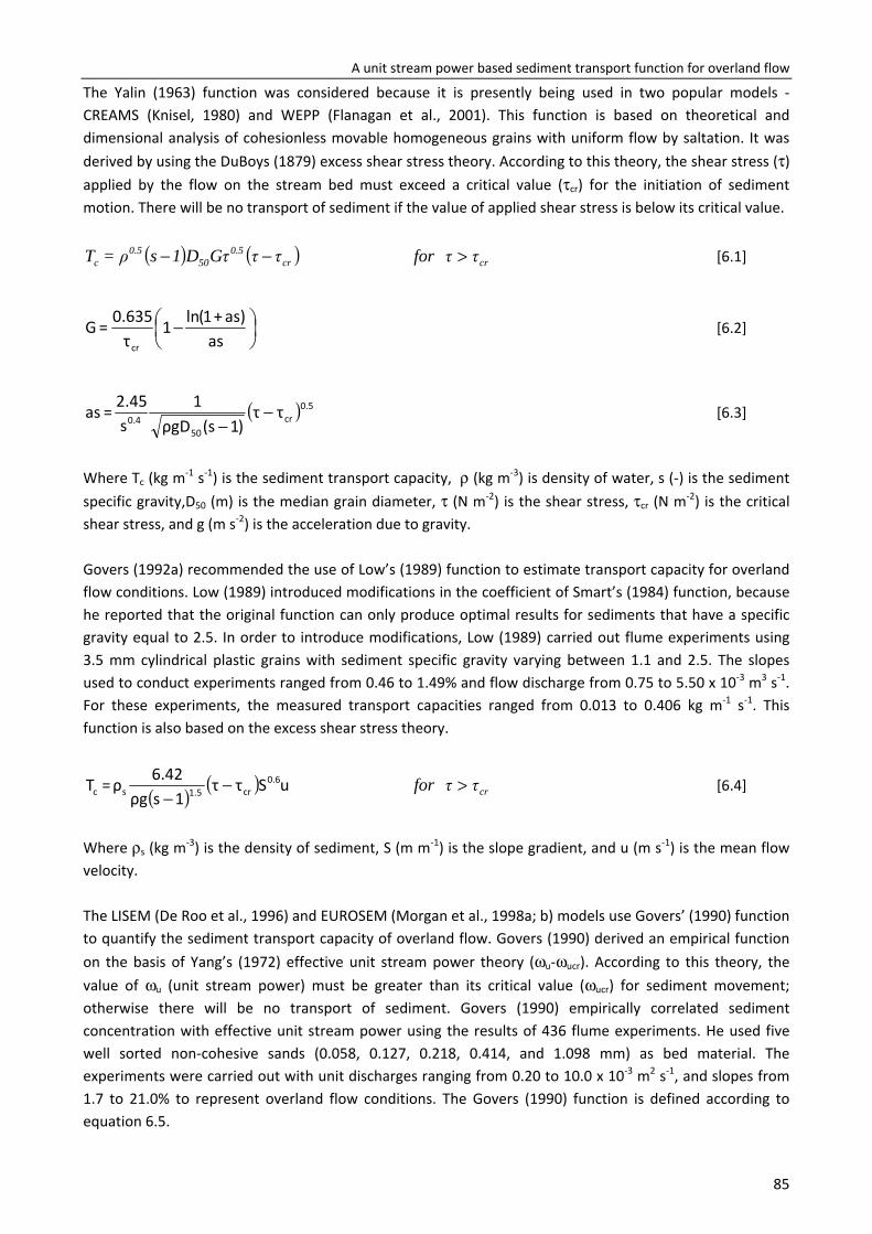
A unit stream power based sediment transport function for overland flow
85
The Yalin (1963) function was considered because it is presently being used in two popular models - CREAMS (Knisel, 1980) and WEPP (Flanagan et al., 2001). This function is based on theoretical and dimensional analysis of cohesionless movable homogeneous grains with uniform flow by saltation. It was derived by using the DuBoys (1879) excess shear stress theory. According to this theory, the shear stress (τ) applied by the flow on the stream bed must exceed a critical value (τcr) for the initiation of sediment motion. There will be no transport of sediment if the value of applied shear stress is below its critical value.
( ) ( )cr0.5
500.5
c ττGτD1sρ=T −− for crττ > [6.1]
−
asas)+1(ln1
τ0.635=G
cr
[6.2]
( )0.5cr
500.4 ττ
)1(sρgD1
s2.45=as −
− [6.3]
Where Tc (kg m-1 s-1) is the sediment transport capacity, ρ (kg m-3) is density of water, s (-) is the sediment specific gravity,D50 (m) is the median grain diameter, τ (N m-2) is the shear stress, τcr (N m-2) is the critical shear stress, and g (m s-2) is the acceleration due to gravity. Govers (1992a) recommended the use of Low’s (1989) function to estimate transport capacity for overland flow conditions. Low (1989) introduced modifications in the coefficient of Smart’s (1984) function, because he reported that the original function can only produce optimal results for sediments that have a specific gravity equal to 2.5. In order to introduce modifications, Low (1989) carried out flume experiments using 3.5 mm cylindrical plastic grains with sediment specific gravity varying between 1.1 and 2.5. The slopes used to conduct experiments ranged from 0.46 to 1.49% and flow discharge from 0.75 to 5.50 x 10⁻³ m3 s-1. For these experiments, the measured transport capacities ranged from 0.013 to 0.406 kg m-1 s-1. This function is also based on the excess shear stress theory.
( ) ( ) uSττ1sρg
6.42ρ=T 0.6cr1.5sc −
− for crττ > [6.4]
Where ρs (kg m-3) is the density of sediment, S (m m-1) is the slope gradient, and u (m s-1) is the mean flow velocity. The LISEM (De Roo et al., 1996) and EUROSEM (Morgan et al., 1998a; b) models use Govers’ (1990) function to quantify the sediment transport capacity of overland flow. Govers (1990) derived an empirical function on the basis of Yang’s (1972) effective unit stream power theory (ωu-ωucr). According to this theory, the value of ωu (unit stream power) must be greater than its critical value (ωucr) for sediment movement; otherwise there will be no transport of sediment. Govers (1990) empirically correlated sediment concentration with effective unit stream power using the results of 436 flume experiments. He used five well sorted non-cohesive sands (0.058, 0.127, 0.218, 0.414, and 1.098 mm) as bed material. The experiments were carried out with unit discharges ranging from 0.20 to 10.0 x 10⁻³ m2 s-1, and slopes from 1.7 to 21.0% to represent overland flow conditions. The Govers (1990) function is defined according to equation 6.5.
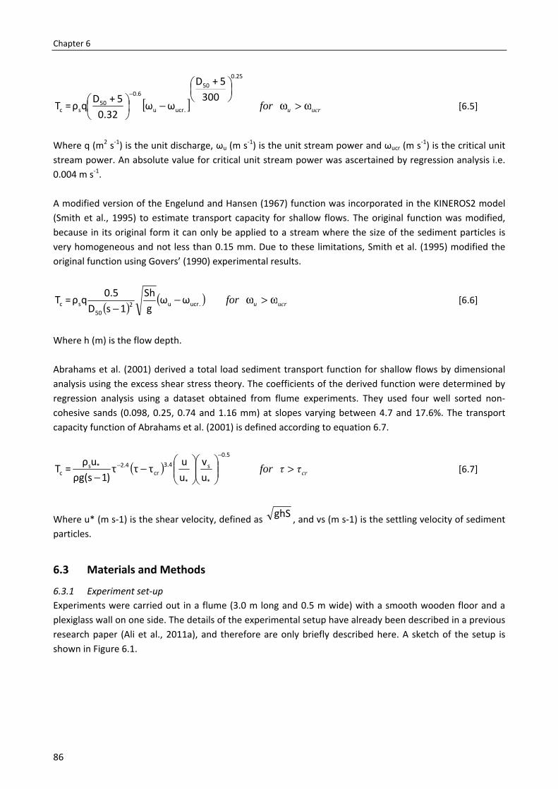
Chapter 6
86
[ ]
0.2550
.ucru
0.650
sc
3005+D
ωω0.32
5+Dqρ=T
−
−
for ucru ω>ω [6.5]
Where q (m2 s-1) is the unit discharge, ωu (m s-1) is the unit stream power and ωucr (m s-1) is the critical unit stream power. An absolute value for critical unit stream power was ascertained by regression analysis i.e. 0.004 m s-1. A modified version of the Engelund and Hansen (1967) function was incorporated in the KINEROS2 model (Smith et al., 1995) to estimate transport capacity for shallow flows. The original function was modified, because in its original form it can only be applied to a stream where the size of the sediment particles is very homogeneous and not less than 0.15 mm. Due to these limitations, Smith et al. (1995) modified the original function using Govers’ (1990) experimental results.
( ) ( ).ucru250
sc ωωgSh
1sD0.5qρ=T −
− for ucru ω>ω [6.6]
Where h (m) is the flow depth. Abrahams et al. (2001) derived a total load sediment transport function for shallow flows by dimensional analysis using the excess shear stress theory. The coefficients of the derived function were determined by regression analysis using a dataset obtained from flume experiments. They used four well sorted non-cohesive sands (0.098, 0.25, 0.74 and 1.16 mm) at slopes varying between 4.7 and 17.6%. The transport capacity function of Abrahams et al. (2001) is defined according to equation 6.7.
( )0.5
*
s
*
3.4cr
2.4*sc u
vuuτττ
)1ρg(suρ=T
−−
−
− for crττ > [6.7]
Where u* (m s-1) is the shear velocity, defined as ghS , and vs (m s-1) is the settling velocity of sediment particles.
6.3 Materials and Methods
6.3.1 Experiment set-up Experiments were carried out in a flume (3.0 m long and 0.5 m wide) with a smooth wooden floor and a plexiglass wall on one side. The details of the experimental setup have already been described in a previous research paper (Ali et al., 2011a), and therefore are only briefly described here. A sketch of the setup is shown in Figure 6.1.
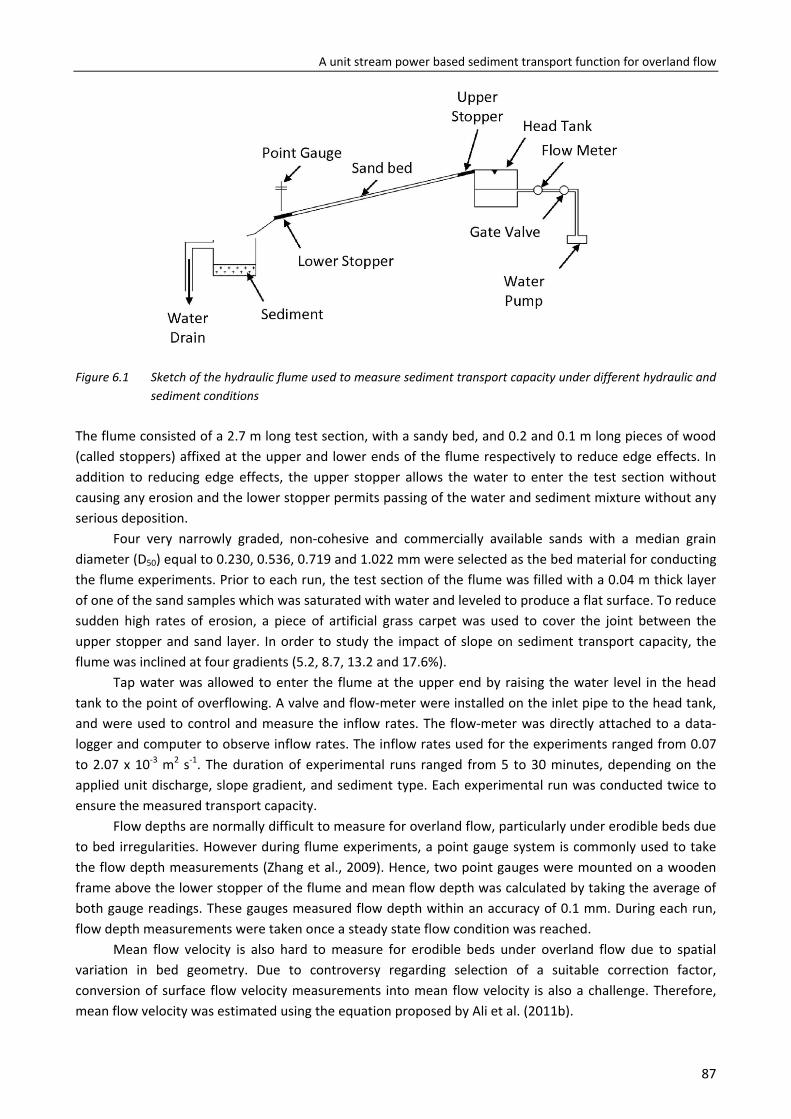
A unit stream power based sediment transport function for overland flow
87
Figure 6.1 Sketch of the hydraulic flume used to measure sediment transport capacity under different hydraulic and
sediment conditions The flume consisted of a 2.7 m long test section, with a sandy bed, and 0.2 and 0.1 m long pieces of wood (called stoppers) affixed at the upper and lower ends of the flume respectively to reduce edge effects. In addition to reducing edge effects, the upper stopper allows the water to enter the test section without causing any erosion and the lower stopper permits passing of the water and sediment mixture without any serious deposition.
Four very narrowly graded, non-cohesive and commercially available sands with a median grain diameter (D50) equal to 0.230, 0.536, 0.719 and 1.022 mm were selected as the bed material for conducting the flume experiments. Prior to each run, the test section of the flume was filled with a 0.04 m thick layer of one of the sand samples which was saturated with water and leveled to produce a flat surface. To reduce sudden high rates of erosion, a piece of artificial grass carpet was used to cover the joint between the upper stopper and sand layer. In order to study the impact of slope on sediment transport capacity, the flume was inclined at four gradients (5.2, 8.7, 13.2 and 17.6%).
Tap water was allowed to enter the flume at the upper end by raising the water level in the head tank to the point of overflowing. A valve and flow-meter were installed on the inlet pipe to the head tank, and were used to control and measure the inflow rates. The flow-meter was directly attached to a data-logger and computer to observe inflow rates. The inflow rates used for the experiments ranged from 0.07 to 2.07 x 10⁻³ m2 s-1. The duration of experimental runs ranged from 5 to 30 minutes, depending on the applied unit discharge, slope gradient, and sediment type. Each experimental run was conducted twice to ensure the measured transport capacity.
Flow depths are normally difficult to measure for overland flow, particularly under erodible beds due to bed irregularities. However during flume experiments, a point gauge system is commonly used to take the flow depth measurements (Zhang et al., 2009). Hence, two point gauges were mounted on a wooden frame above the lower stopper of the flume and mean flow depth was calculated by taking the average of both gauge readings. These gauges measured flow depth within an accuracy of 0.1 mm. During each run, flow depth measurements were taken once a steady state flow condition was reached.
Mean flow velocity is also hard to measure for erodible beds under overland flow due to spatial variation in bed geometry. Due to controversy regarding selection of a suitable correction factor, conversion of surface flow velocity measurements into mean flow velocity is also a challenge. Therefore, mean flow velocity was estimated using the equation proposed by Ali et al. (2011b).
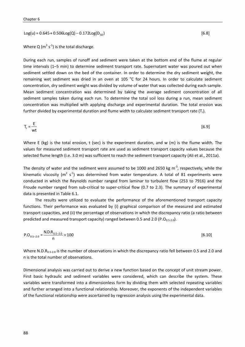
Chapter 6
88
)Log(D0.172Log(Q)0.506+0.645=Log(u) 50− [6.8]
Where Q (m3 s-1) is the total discharge. During each run, samples of runoff and sediment were taken at the bottom end of the flume at regular time intervals (1–5 min) to determine sediment transport rate. Supernatant water was poured out when sediment settled down on the bed of the container. In order to determine the dry sediment weight, the remaining wet sediment was dried in an oven at 105 oC for 24 hours. In order to calculate sediment concentration, dry sediment weight was divided by volume of water that was collected during each sample. Mean sediment concentration was determined by taking the average sediment concentration of all sediment samples taken during each run. To determine the total soil loss during a run, mean sediment concentration was multiplied with applying discharge and experimental duration. The total erosion was further divided by experimental duration and flume width to calculate sediment transport rate (Tr).
wtE=Tr [6.9]
Where E (kg) is the total erosion, t (sec) is the experiment duration, and w (m) is the flume width. The values for measured sediment transport rate are used as sediment transport capacity values because the selected flume length (i.e. 3.0 m) was sufficient to reach the sediment transport capacity (Ali et al., 2011a). The density of water and the sediment were assumed to be 1000 and 2650 kg m-3, respectively, while the kinematic viscosity (m2 s-1) was determined from water temperature. A total of 81 experiments were conducted in which the Reynolds number ranged from laminar to turbulent flow (253 to 7916) and the Froude number ranged from sub-critical to super-critical flow (0.7 to 2.3). The summary of experimental data is presented in Table 6.1.
The results were utilized to evaluate the performance of the aforementioned transport capacity functions. Their performance was evaluated by (i) graphical comparison of the measured and estimated transport capacities, and (ii) the percentage of observations in which the discrepancy ratio (a ratio between predicted and measured transport capacity) ranged between 0.5 and 2.0 (P.O0.5-2.0).
100n
R.D.N=O.P 2.00.5
2.00.5 ×−− [6.10]
Where N.D.R0.5-2.0 is the number of observations in which the discrepancy ratio fell between 0.5 and 2.0 and n is the total number of observations. Dimensional analysis was carried out to derive a new function based on the concept of unit stream power. First basic hydraulic and sediment variables were considered, which can describe the system. These variables were transformed into a dimensionless form by dividing them with selected repeating variables and further arranged into a functional relationship. Moreover, the exponents of the independent variables of the functional relationship were ascertained by regression analysis using the experimental data.
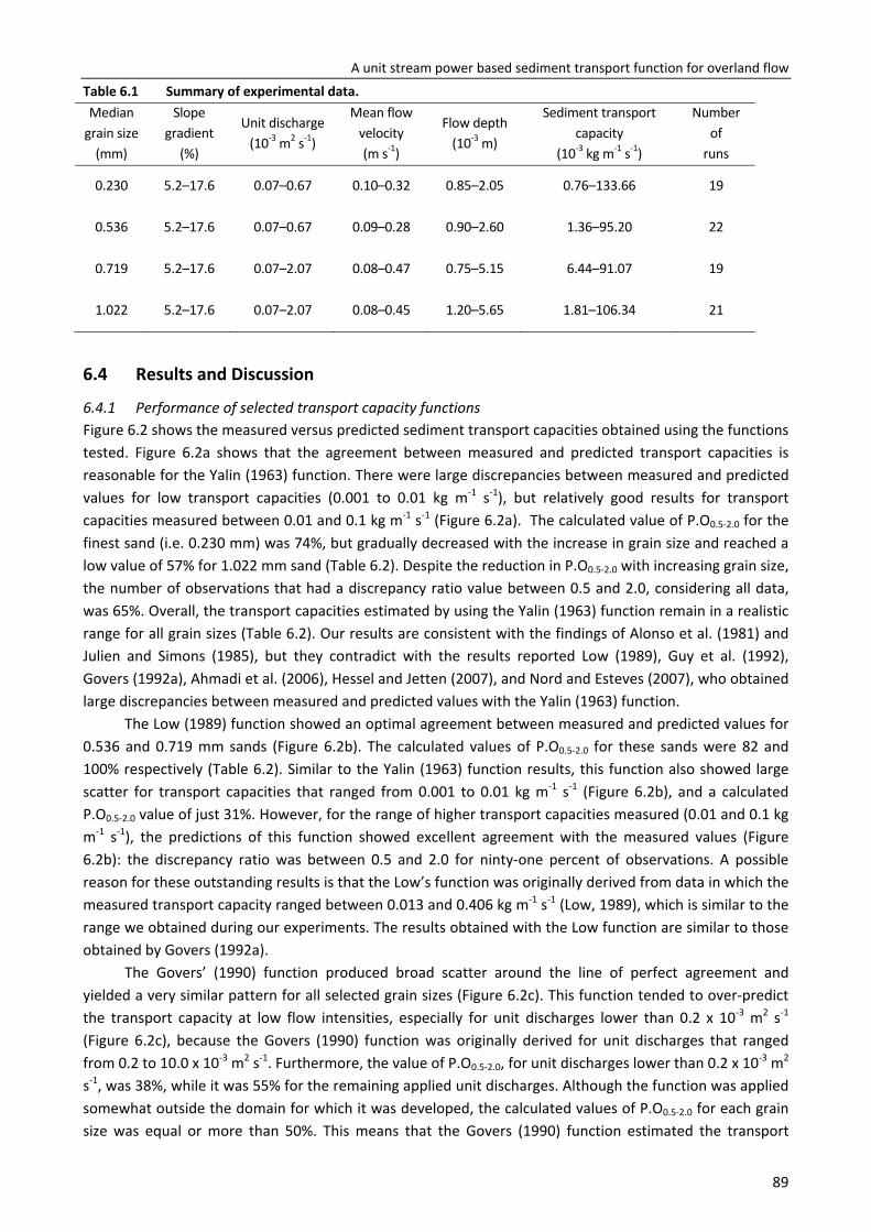
A unit stream power based sediment transport function for overland flow
89
Table 6.1 Summary of experimental data. Median
grain size (mm)
Slope gradient
(%)
Unit discharge (10-3 m2 s-1)
Mean flow velocity (m s-1)
Flow depth (10-3 m)
Sediment transport capacity
(10-3 kg m-1 s-1)
Number of
runs
0.230 5.2–17.6 0.07–0.67 0.10–0.32 0.85–2.05 0.76–133.66 19
0.536 5.2–17.6 0.07–0.67 0.09–0.28 0.90–2.60 1.36–95.20 22
0.719 5.2–17.6 0.07–2.07 0.08–0.47 0.75–5.15 6.44–91.07 19
1.022 5.2–17.6 0.07–2.07 0.08–0.45 1.20–5.65 1.81–106.34 21
6.4 Results and Discussion
6.4.1 Performance of selected transport capacity functions Figure 6.2 shows the measured versus predicted sediment transport capacities obtained using the functions tested. Figure 6.2a shows that the agreement between measured and predicted transport capacities is reasonable for the Yalin (1963) function. There were large discrepancies between measured and predicted values for low transport capacities (0.001 to 0.01 kg m-1 s-1), but relatively good results for transport capacities measured between 0.01 and 0.1 kg m-1 s-1 (Figure 6.2a). The calculated value of P.O0.5-2.0 for the finest sand (i.e. 0.230 mm) was 74%, but gradually decreased with the increase in grain size and reached a low value of 57% for 1.022 mm sand (Table 6.2). Despite the reduction in P.O0.5-2.0 with increasing grain size, the number of observations that had a discrepancy ratio value between 0.5 and 2.0, considering all data, was 65%. Overall, the transport capacities estimated by using the Yalin (1963) function remain in a realistic range for all grain sizes (Table 6.2). Our results are consistent with the findings of Alonso et al. (1981) and Julien and Simons (1985), but they contradict with the results reported Low (1989), Guy et al. (1992), Govers (1992a), Ahmadi et al. (2006), Hessel and Jetten (2007), and Nord and Esteves (2007), who obtained large discrepancies between measured and predicted values with the Yalin (1963) function.
The Low (1989) function showed an optimal agreement between measured and predicted values for 0.536 and 0.719 mm sands (Figure 6.2b). The calculated values of P.O0.5-2.0 for these sands were 82 and 100% respectively (Table 6.2). Similar to the Yalin (1963) function results, this function also showed large scatter for transport capacities that ranged from 0.001 to 0.01 kg m-1 s-1 (Figure 6.2b), and a calculated P.O0.5-2.0 value of just 31%. However, for the range of higher transport capacities measured (0.01 and 0.1 kg m-1 s-1), the predictions of this function showed excellent agreement with the measured values (Figure 6.2b): the discrepancy ratio was between 0.5 and 2.0 for ninty-one percent of observations. A possible reason for these outstanding results is that the Low’s function was originally derived from data in which the measured transport capacity ranged between 0.013 and 0.406 kg m-1 s-1 (Low, 1989), which is similar to the range we obtained during our experiments. The results obtained with the Low function are similar to those obtained by Govers (1992a).
The Govers’ (1990) function produced broad scatter around the line of perfect agreement and yielded a very similar pattern for all selected grain sizes (Figure 6.2c). This function tended to over-predict the transport capacity at low flow intensities, especially for unit discharges lower than 0.2 x 10⁻³ m2 s-1 (Figure 6.2c), because the Govers (1990) function was originally derived for unit discharges that ranged from 0.2 to 10.0 x 10⁻³ m2 s-1. Furthermore, the value of P.O0.5-2.0, for unit discharges lower than 0.2 x 10⁻³ m2 s-1, was 38%, while it was 55% for the remaining applied unit discharges. Although the function was applied somewhat outside the domain for which it was developed, the calculated values of P.O0.5-2.0 for each grain size was equal or more than 50%. This means that the Govers (1990) function estimated the transport
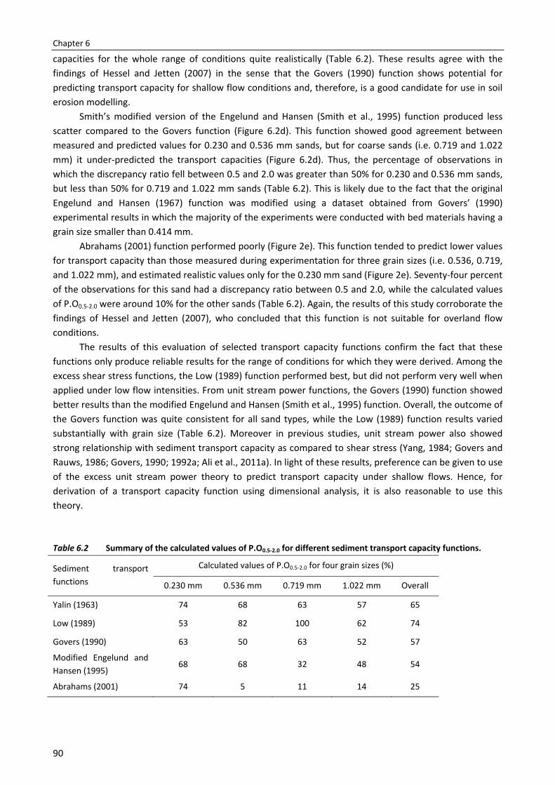
Chapter 6
90
capacities for the whole range of conditions quite realistically (Table 6.2). These results agree with the findings of Hessel and Jetten (2007) in the sense that the Govers (1990) function shows potential for predicting transport capacity for shallow flow conditions and, therefore, is a good candidate for use in soil erosion modelling.
Smith’s modified version of the Engelund and Hansen (Smith et al., 1995) function produced less scatter compared to the Govers function (Figure 6.2d). This function showed good agreement between measured and predicted values for 0.230 and 0.536 mm sands, but for coarse sands (i.e. 0.719 and 1.022 mm) it under-predicted the transport capacities (Figure 6.2d). Thus, the percentage of observations in which the discrepancy ratio fell between 0.5 and 2.0 was greater than 50% for 0.230 and 0.536 mm sands, but less than 50% for 0.719 and 1.022 mm sands (Table 6.2). This is likely due to the fact that the original Engelund and Hansen (1967) function was modified using a dataset obtained from Govers’ (1990) experimental results in which the majority of the experiments were conducted with bed materials having a grain size smaller than 0.414 mm.
Abrahams (2001) function performed poorly (Figure 2e). This function tended to predict lower values for transport capacity than those measured during experimentation for three grain sizes (i.e. 0.536, 0.719, and 1.022 mm), and estimated realistic values only for the 0.230 mm sand (Figure 2e). Seventy-four percent of the observations for this sand had a discrepancy ratio between 0.5 and 2.0, while the calculated values of P.O0.5-2.0 were around 10% for the other sands (Table 6.2). Again, the results of this study corroborate the findings of Hessel and Jetten (2007), who concluded that this function is not suitable for overland flow conditions.
The results of this evaluation of selected transport capacity functions confirm the fact that these functions only produce reliable results for the range of conditions for which they were derived. Among the excess shear stress functions, the Low (1989) function performed best, but did not perform very well when applied under low flow intensities. From unit stream power functions, the Govers (1990) function showed better results than the modified Engelund and Hansen (Smith et al., 1995) function. Overall, the outcome of the Govers function was quite consistent for all sand types, while the Low (1989) function results varied substantially with grain size (Table 6.2). Moreover in previous studies, unit stream power also showed strong relationship with sediment transport capacity as compared to shear stress (Yang, 1984; Govers and Rauws, 1986; Govers, 1990; 1992a; Ali et al., 2011a). In light of these results, preference can be given to use of the excess unit stream power theory to predict transport capacity under shallow flows. Hence, for derivation of a transport capacity function using dimensional analysis, it is also reasonable to use this theory.
Table 6.2 Summary of the calculated values of P.O0.5-2.0 for different sediment transport capacity functions.
Sediment transport functions
Calculated values of P.O0.5-2.0 for four grain sizes (%)
0.230 mm 0.536 mm 0.719 mm 1.022 mm Overall
Yalin (1963) 74 68 63 57 65
Low (1989) 53 82 100 62 74
Govers (1990) 63 50 63 52 57
Modified Engelund and Hansen (1995)
68 68 32 48 54
Abrahams (2001) 74 5 11 14 25
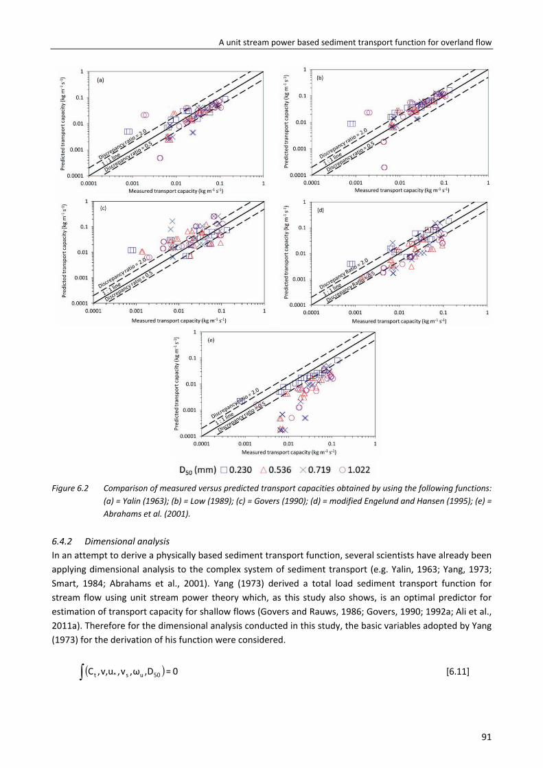
A unit stream power based sediment transport function for overland flow
91
Figure 6.2 Comparison of measured versus predicted transport capacities obtained by using the following functions: (a) = Yalin (1963); (b) = Low (1989); (c) = Govers (1990); (d) = modified Engelund and Hansen (1995); (e) = Abrahams et al. (2001).
6.4.2 Dimensional analysis In an attempt to derive a physically based sediment transport function, several scientists have already been applying dimensional analysis to the complex system of sediment transport (e.g. Yalin, 1963; Yang, 1973; Smart, 1984; Abrahams et al., 2001). Yang (1973) derived a total load sediment transport function for stream flow using unit stream power theory which, as this study also shows, is an optimal predictor for estimation of transport capacity for shallow flows (Govers and Rauws, 1986; Govers, 1990; 1992a; Ali et al., 2011a). Therefore for the dimensional analysis conducted in this study, the basic variables adopted by Yang (1973) for the derivation of his function were considered.
( ) 0=D,ω,v,uv,,C 50us*t [6.11]
Chapter 6
92
It is generally assumed that under overland flow conditions sand particles are normally rolling, sliding and saltating over the bed (Lu et al., 1989), instead of moving as a suspended load. Hence for bed-load estimation, the variable of total sediment concentration (Ct) was replaced by volumetric bed-load discharge (qb). In addition, mean flow velocity (u) was substituted for kinematic viscosity (v), because flow velocity remains dynamic due to continuous variation in local slope and has a strong impact on sediment transport (Ali et al., 2011a). Equation 6.11, therefore, becomes:
( ) 0=D,ω,v,uu,,q 50us*b [6.12]
Where qb [L2 T-1] is the volumetric bed-load discharge, u [L T-1] is the mean flow velocity, u* [L T-1] is the shear velocity, vs [L T-1] is the settling velocity, ωu [L T-1] is the unit stream power, and D50 [L] is median grain diameter. Median grain size (D50) and settling velocity (vs) were considered as repeating variables, because the system is described by two fundamental dimensions (i.e. L and T). Apart from this, the selected repeating variables contain all the dimensions which are involved in the system and cannot form a dimensionless group. With these changes, Equation 6.12 becomes:
0=vω
,vu,
vu,
vD
q
s
u
ss
*
s50
b
[6.13]
By applying the Buckingham’s π theorem, than the functional equation can be written as equation 6.14.
s
u
ss
*
s50
b
vω
,vu,
vu=
vD
q [6.14]
Yang (1973) used the concept of effective unit stream power ( ucru ωω − ) as an incipient motion criteria in
his function. The difference between the unit stream power and critical unit stream power (ωucr) is actually the available flow energy, which is used for the transport of sediment. According to this concept, the value of ωu must be greater than its critical value for the initiation of sediment. The same concept was utilized in this study to modify the above functional relation (Equation 6.14).
−
s
cru
s
u
ss
*
s50
b
v
ω
vω
,vu,
vu
=vD
q [6.15]
By defining,
s50
b
vD
q=φ
Where φ is the dimensionless bed-load transport rate. Now, Equation 6.15 can be written as Equation 6.16.
A unit stream power based sediment transport function for overland flow
93
−
s
cru
s
u
ss
*
v
ω
vω
,vu,
vu
=φ [6.16]
Similar to Yang (1973), the functional relationship can be expressed as a power product.
d
s
ucr
s
uc
s
b
s
*
vω
vω
vu
vu
a=φ
−
[6.17]
Where a, b, c and d are the coefficients, which were worked out using experimental data by regression analysis. Using the data from the present analysis, Equation 6.17 becomes:
−
s
ucr
s
u0.62
s
1.64
s
*
vω
vω
vu
vu
3.63=φ [6.18]
Govers (1990) empirically derived a value for critical unit stream power: 0.004 m s-1 for the sediment particles ranged from 0.058 to 0.218 mm. The same value was used here for the initiation of sediment, because the sediment particles considered in this study were much coarser than the sediment particles considered by Govers (1990). Figure 6.3 shows the agreement between the measured and predicted transport capacities predicted by using Equation 6.18 for four grain sizes.
Figure 6.3 Comparison between the measured values and predicted transport capacities using Equation 6.18.
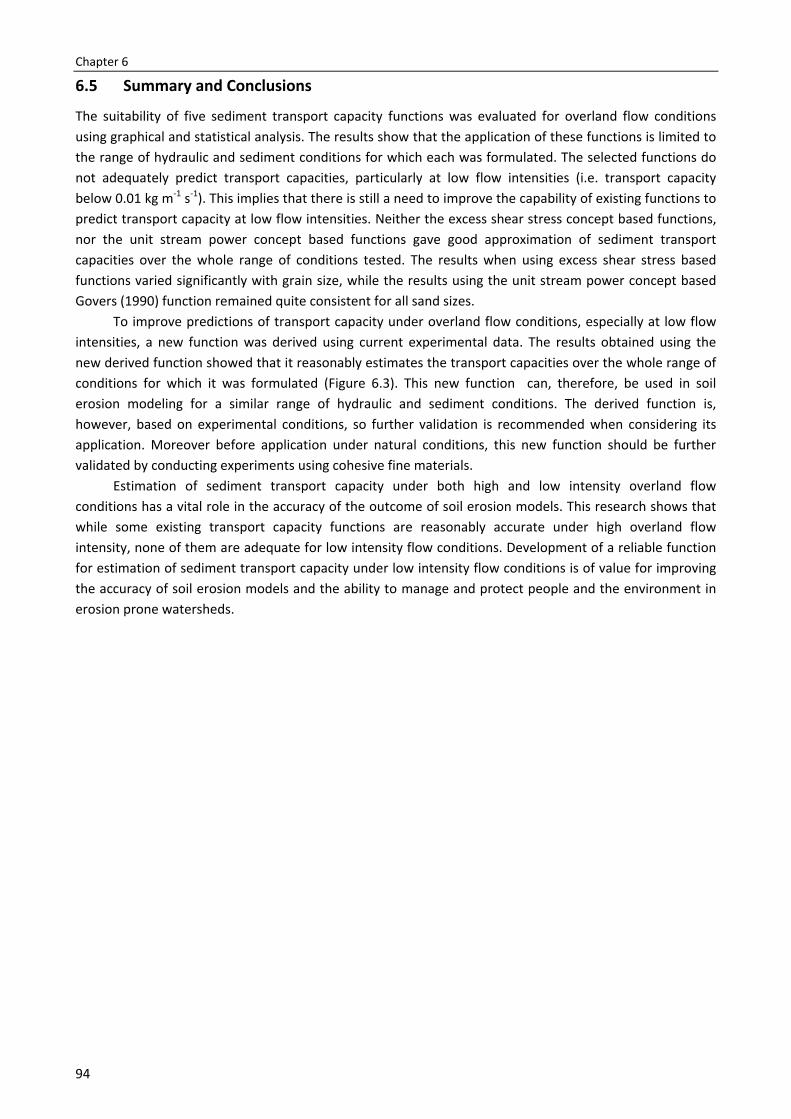
Chapter 6
94
6.5 Summary and Conclusions
The suitability of five sediment transport capacity functions was evaluated for overland flow conditions using graphical and statistical analysis. The results show that the application of these functions is limited to the range of hydraulic and sediment conditions for which each was formulated. The selected functions do not adequately predict transport capacities, particularly at low flow intensities (i.e. transport capacity below 0.01 kg m-1 s-1). This implies that there is still a need to improve the capability of existing functions to predict transport capacity at low flow intensities. Neither the excess shear stress concept based functions, nor the unit stream power concept based functions gave good approximation of sediment transport capacities over the whole range of conditions tested. The results when using excess shear stress based functions varied significantly with grain size, while the results using the unit stream power concept based Govers (1990) function remained quite consistent for all sand sizes.
To improve predictions of transport capacity under overland flow conditions, especially at low flow intensities, a new function was derived using current experimental data. The results obtained using the new derived function showed that it reasonably estimates the transport capacities over the whole range of conditions for which it was formulated (Figure 6.3). This new function can, therefore, be used in soil erosion modeling for a similar range of hydraulic and sediment conditions. The derived function is, however, based on experimental conditions, so further validation is recommended when considering its application. Moreover before application under natural conditions, this new function should be further validated by conducting experiments using cohesive fine materials.
Estimation of sediment transport capacity under both high and low intensity overland flow conditions has a vital role in the accuracy of the outcome of soil erosion models. This research shows that while some existing transport capacity functions are reasonably accurate under high overland flow intensity, none of them are adequate for low intensity flow conditions. Development of a reliable function for estimation of sediment transport capacity under low intensity flow conditions is of value for improving the accuracy of soil erosion models and the ability to manage and protect people and the environment in erosion prone watersheds.

Chapter 7
Synthesis

97
Synthesis
7.1 Problem definition, main aim and research questions
Soil erosion is a global ecological problem that has adverse impacts not only on agriculture production, but also on water conveyance and water storage facilities (Lal and Stewart, 1990; Pimentel et al., 1995; Lal, 1998; Yang et al., 2003). World-wide, sustainability of existing reservoirs is threatened by sedimentation resulting from soil erosion processes, especially in Pakistan, China and Turkey (Sloff, 1997). In Pakistan the annual storage depletion rate of existing reservoirs (e.g. Tarbela and Mangla) is in general higher than the global annual depletion rate of 1% (TAMS, 1998; Ali et al., 2006). In order to reduce the annual storage depletion rate of these reservoirs, several efforts have been made by adopting different reservoir operation strategies such as raising of the Minimum operation Level (MoL) and flushing (TAMS, 1998; DBC, 2007). However, the successful application of these strategies sometimes becomes debatable due to limited annual water availability, high sediment inflows, the large size of the reservoir and the characteristics of the outlets (Qian, 1982; White, 2000; Emamgholizadeh and Samadi, 2008). Therefore alternative strategies are needed to preserve reservoir life-span – in particular reducing sediment inflow. Such strategies require estimation of areas susceptible to erosion in order to implement appropriate soil and water conservation practices. This thesis has focussed on improving the effectiveness of soil erosion modelling through increasing the accuracy of estimating transport capacity.
In Chapter 2 of this thesis, both the raising of MoL and flushing techniques were considered for reduction of the annual storage depletion rate of the planned Basha reservoir in north Pakistan. The results showed that the adoption of a gradual raising of MoL retarded the sediment delta movement towards the dam body, but at the same time increased the annual storage depletion rate. Similarly, flushing operations also exhibited some positive impacts on the life-span of the planned Basha reservoir, but also pose a serious threat for downstream reservoirs, as well as reducing the project benefits since power-houses are shutdown during the flushing period. Hence, these strategies are not the best sediment management options for the planned Basha reservoir.
In-addition to the just mentioned reservoir operation strategies, the storage depletion rate of a reservoir can also be reduced by limiting the sediment inflow rate, which is generally accomplished by implementing soil and water conservation practices in the upstream catchment area (Huang and Zhang, 2004; Solaimani et al., 2009; Minella et al., 2009). In the case of the Basha reservoir, its life-span would be more than 100 years (which is 40–50 years more than the normal estimated life), if the current sediment inflow rate could be reduced by 50% through executing watershed management projects in the catchment area (Chapter 2).
In order to know where soil and water conservation practices in catchments will be most effective, areas with high erosion potential need to be identified. For the identification of such hot-spots, spatially distributed soil erosion models are available, but the prediction capability of existing models is still low (Schoorl et al., 2000; Jetten et al., 2003; Hessel et al., 2006; Vigiak et al., 2006). The poor spatial erosion predictions can be attributed to the use of empirical flow velocity equations (i.e. Manning and Darcy-Weisbach equations) and inappropriate sediment transport capacity functions (Yalin, 1963; Low, 1989; Smith et al., 1995). Precise quantification of sediment transport capacity is necessary for the estimation of spatial variation of soil erosion because detachment and deposition rates (sources of sediment flow) depend strongly on it (Foster and Meyer, 1972). In order to more precisely estimate the spatial erosion variation, it is necessary to improve understanding of the factors and processes that are involved in sediment transport under overland flow conditions.
The main objective of this study was, therefore, to develop a theoretical and mathematical framework for the precise quantification of sediment transport capacity, which plays a vital role in the
Chapter 7
98
accurate estimation of highly erodible areas in a catchment. In order to achieve this objective, flume experiments were carried out under controlled conditions, where sediment transport controlling factors could be precisely measured. The results are briefly discussed below by research question. Gained knowledge is highlighted and current findings are compared with previous findings. In addition, study limitations and areas for future research are also outlined before drawing final conclusions. The outcomes of this thesis project can be used by erosion modellers working with existing spatially distributed soil erosion models to generate more realistic results through use of the most appropriate functions for the location being studied.
7.2 Suitability of existing approaches and functions used for mean flow velocity and
sediment transport capacity quantification For the accurate assessment of soil erosion, the choice of an appropriate sediment transport capacity function is vital to soil erosion modelling. Wrong selection of a transport capacity function may mislead the identification of highly erodible areas in a watershed, which would become the cause of the failure of a watershed management project. For the precise quantification of sediment transport capacity, accurate estimation of mean flow velocity is essential. In this section, our findings with respect to existing approaches used for the estimation of mean flow velocity and sediment transport capacity, and their limitations are discussed.
7.2.1 Mean flow velocity The Manning and Darcy-Weisbach flow velocity equations are generally used in spatially distributed soil erosion models for the quantification of mean flow velocity (KINEROS2, Smith et al., 1995; LISEM, De Roo et al., 1996; WEPP, Flanagan et al., 2001), but their application is questionable for the following reasons.
(i) According to the Manning and Darcy-Weisbach equations, mean flow velocity increases with slope
gradient, but experimental findings show that the slope has a non-significant effect on mean flow velocity under overland flow conditions (Govers, 1992b; Nearing et al., 1997; Takken et al., 1998; Nearing et al., 1999; Gimenez and Govers, 2001). The reason is that in overland flow over an erodible soil, the available flow energy is preferentially used for the detachment and transport of sediment, instead of increasing the flow velocity. Our experimental findings (Chapter 4) further confirm previous literature findings.
(ii) Mean flow velocity increases with increasing hydraulic radius in both equations. Because flow width
for overland flow conditions is much larger than flow depth, the hydraulic radius is generally considered equivalent to flow depth. Thus, their application becomes questionable for overland flow, since it is hard to observe flow depth in the field due to spatial variation of the bed geometry (Jayawardena and Bhuiyan, 1999), which makes flow depth a highly variable parameter. Moreover, standard equipment for measurement of overland flow depth is non-available (Stroosnijder, 2005).
(iii) In the flow equations, the mean flow velocity depends on the value of the roughness coefficient (n in
the Manning equation; f in the Darcy-Weisbach equation). The values for these coefficients are available in the literature for different bed grain sizes, but for stream flow conditions only (Chaudhry, 2007). It appears to be difficult to estimate values for these roughness coefficients under overland flow conditions since bed roughness is very dynamic due to a continuous variation in bed geometry (Govers, 1992b; Gimenez and Govers, 2001).
Synthesis
99
In view of the shortcomings of the existing approaches, it is imperative to better understand the processes that control and affect the mean flow velocity under overland flow conditions. Furthermore, a mathematical framework is also needed, which can be used to precisely estimate the variation of mean flow velocity with flow discharge, bed material grain size, and bed geometry.
7.2.2 Sediment transport capacity In order to select a suitable sediment transport capacity function for overland flow, credible information is needed regarding the physical basis and application boundaries of existing functions, and their suitability under different overland flow conditions.
During soil erosion modelling, sediment transport capacity is usually estimated by adopting functions that were derived either for stream flow conditions or for overland flow conditions (e.g. Yalin, 1963; Yang, 1973; Low, 1989; Govers, 1990; 1992a; Smith et al., 1995; Abrahams et al., 2001). The available functions can be sub-divided into bed load and total load functions. Because the stream flow functions are derived for mild slopes, high discharges, and substantial flow depths, their application becomes debatable for overland flow, where flow conditions are entirely different. The majority of the available overland flow sediment transport capacity functions are of empirical nature and were derived by using small laboratory plot results that might not be representative for field conditions (Govers, 1990; Everaert, 1991; Govers, 1992a; Jayawardena and Bhuiyan, 1999; Zhang et al., 2009).
In the literature, several scientists have already evaluated the performance of the many sediment transport capacity functions for a wide range of overland conditions. They always recommend either a bed load stream flow function or an overland flow function (Alonso et al., 1981; Low, 1989; Govers, 1992a; Guy et al., 1992; Ahmadi et al., 2006; Hessel and Jetten, 2007; Nord and Esteves, 2007). Furthermore, the recommended functions are based on either shear stress concept or unit stream power concept. Given the performance of existing functions under different range of conditions (Chapters 3), unit stream power concept based transport capacity functions (i.e. Govers, 1990; 1992a) can be used for wide range of conditions i.e. slopes ranged from mild to very steep (0.017 to 2.5 m m-1) and bed materials from clay to coarse sands (Govers, 1992a; Hessel and Jetten, 2007; Nord and Esteves, 2007). Whereas, shear stress concept based functions (i.e. Yalin, 1963; Low, 1989) may only be applicable to a limited range of slopes and bed materials (Chapters 3). In the light of available information regarding the performance of functions, it can be concluded that the functions can only estimate transport capacities reasonably for the range of conditions, for which they were formulated (Chapter 3).
Thus, a single function cannot be recommended globally. These limitations can be reduced, however, by using physical parameters that affect and control the transport of sediment under overland flow conditions. For this purpose, further work in this project focussed on understanding the processes involved in transport of sediment (Chapter 5).
7.3 Factors affecting and controlling the mean flow velocity and sediment transport capacity
Given the shortcomings in existing approaches (Section 7.2), the main focus for this thesis research was to find out how to precisely estimate mean flow velocity and sediment transport capacity of a particular discharge at a certain slope for overland flow conditions. For this purpose, the effect of different hydraulic and sediment parameters like flow discharge, slope gradient, and median grain diameter on mean flow velocity and sediment transport capacity was studied using a novel laboratory setup where conditions could be well controlled. Results (Chapters 4 and 5) are concisely discussed here.
Chapter 7
100
Flow discharge showed a pronounced impact on both mean flow velocity and sediment transport capacity. Experimental results revealed that mean flow velocity increased with flow discharge at a constant slope, leading to a growth in sediment transport capacity (Chapters 4 and 5), due to an increase of the kinetic energy of the flowing water.
Slope gradient had a strong influence on sediment transport capacity (Chapter 5). The latter gradually increased with the increase in slope gradient for a particular flow discharge. On the contrary, the effect of slope gradient on mean flow velocity was found to be highly non-significant (Chapter 4). This is because the available flow energy was preferentially dissipated for the detachment and transport of sediment particles from the soil mass, instead of increasing mean flow velocity as was previously assumed (Gimenez and Govers, 2002).
Like flow discharge, median grain diameter also showed a strong impact on both mean flow velocity and sediment transport capacity. The experiments showed that both were progressively reduced with the increase of grain size for a particular flow discharge at a certain slope (Chapters 4 and 5). The possible reason is that the energy dissipation of a particular discharge for transporting sediment particles increases with grain size due to the increase in bed roughness. The significant impact of grain size on mean flow velocity contradict with the findings of Govers (1992), Takken et al. (1998) and Gimenez and Govers (2001).
Mean flow velocity exhibited a strong relationship with sediment transport capacity. The flume measurements showed that the sediment transport capacity increased with mean flow velocity at a constant slope (Chapter 5). This relationship between mean flow velocity and sediment transport capacity was strongly dependent on slope gradient, which contradicts the findings of previous scientists (Guy et al., 1990; Zhang et al., 2009). The most likely reason for this contradiction is that they studied the impact of mean flow velocity on sediment transport capacity under non-erodible beds, where mean flow velocity gradually increases with slope gradient due to insignificant variation in bed roughness (Foster et al., 1984; Abrahams et al., 1996; Gimenez and Govers, 2001; Zhang et al., 2009).
In this study, the experiments were done with erodible beds, and bed morphology varied substantially with grain size for a particular discharge at a certain slope (Chapter 4). For example, narrow and small rills were observed for coarse sand due to its higher bed roughness as compared to fine sand (Figures 4.3 and 4.4). With the variation in bed geometry, the local flow velocity also varied greatly, which eventually had a strong impact on sediment transport capacity. Hence, lower values of mean flow velocity and transport capacity were observed for coarse sand at a certain slope and discharge than for fine sand.
The results of this study has shown that more research is needed to completely understand the effect of different hydraulic and sediment parameters on mean flow velocity and sediment transport capacity. Moreover, the results also revealed the fact that the dynamics of overland flow on erodible surfaces is significantly different than dynamics on non-erodible surfaces. Hence the application of theoretical concepts, which were derived for non-erodible beds, on a natural hellslope may produce errors.
7.4 Development of a function for the quantification of mean flow velocity and sediment transport capacity
7.4.1 Estimation of mean flow velocity Given the strong impact of flow discharge and grain size on mean flow velocity (Section 7.3), a new empirical equation for mean flow velocity was derived by regression analysis (Chapter 4). The performance of the proposed equation was evaluated by using different statistical techniques on five datasets from the literature. Those datasets were also collected for non-cohesive sands (Aziz and Scott, 1989; Li et al., 1996; Li and Abrahams, 1997; Hu and Abrahams, 2005; Zhang et al., 2010b). The derived equation showed a reasonable agreement between the observed and predicted mean flow velocities (Chapter 4; Figure 4.8).
Synthesis
101
7.4.2 Sediment transport capacity function For the development of a sediment transport capacity function, the fundamental questions are 1) which composite force predictor has the strongest relationship with transport capacity? and 2) how does this relationship vary with the increase or decrease of grain size?
The measured sediment transport capacity was well related to three selected composite predictors (i.e. stream power, unit stream power and effective stream power), but showed a poor relation with shear stress (Chapter 5). The possible reason for the poor performance of shear stress is that the part of shear stress (i.e. form shear stress) is used to detach the soil particles from the soil mass, instead of transporting the sediment particles (Chapter 5). Based on further analysis, preference was given to the theory of unit stream power over the other selected composite force predictors. This is because our experiments discovered that unit stream power not only showed a strong relationship with transport capacity, but also it was found independent of grain size effect (Chapter 5). The non-significant impact of grain size on the relationship between sediment transport capacity and unit stream power was somewhat surprising, because normally grain size is expected to have a strong impact on sediment transport capacity (section 7.3). Indeed, grain size had a significant impact on the relationship between sediment transport capacity and the other selected composite predictors. Moreover, the absence of an influence of grain size on the relationship between unit stream power and sediment transport capacity is contradict with previous findings for overland flow (Govers and Rauws, 1986; Govers, 1990; 1992a). This lack of influence of grain size was exploited by deriving a more generally applicable equation for sediment transport capacity, which uses unit stream power as the driving force for sediment transport.
Given the ability of the unit stream power concept to quantify the sediment transport capacity for overland flow conditions (Chapters 5), a new function was derived by dimensional analysis on the basis of experimental results (Chapters 6). In this function, the energy used for the initiation of sediment transport was analysed in terms of effective unit stream power, which is actually a difference between unit stream power and its critical value. According to this approach, the value of unit stream power must exceed its critical value for sediment motion, otherwise there will be no transport of sediment. In addition to this, mean flow velocity and shear velocity were also considered to ascertain the amount of the energy exerted by the rate of discharge on the bed at a particular slope.
7.5 Limitations of the study
As the experiments were carried out in a small flume (i.e. 3.0 m long and 0.5 m wide) by using a certain range of flow discharges, slope gradients and grain sizes, the results might not fully encompass the hillslope conditions. Therefore the limitations of the experimental work are briefly discussed here. One of the limitations is the thin layer of sand (i.e. 4.0 cm) that was used for the evolution of bed morphology for each combination of applied flow discharge and slope gradient. This means that the results of this study may only be valid for similar conditions, where depth of the rills is less than 4.0 cm. Furthermore, the selected non-cohesive sands do not completely behave like cohesive soils. For example, a non-cohesive sand does not reflect the aggregate effect on sediment transport capacity. Besides this, the selected range of flow discharges and slope gradients does not fully represent the flow conditions of hillslope.
The theoretical and mathematical approaches presented in this thesis are based on flume observations of limited scale (as described above) which implies that these should be only cautiously applied outside the domain for which they were actually derived i.e. unit discharge ranged from 0.07 to 2.07 x 10⁻³ m2 s-1, slope gradient from 5.2 to 17.6%, median grain size from 0.233 to 1.022 mm, mean flow velocity from 0.08 to 0.47 m s-1, sediment transport capacity from 0.76 to 133.66 x 10⁻³ kg m-1 s-1, and Reynolds number from 253 to 7916.
Chapter 7
102
Although the proposed mathematical approaches showed an optimal fit through the data-points (Figures 5.6 and 6.3), it needs to be validated for cohesive soils like clay loam and silt loam soils. Moreover, it is also need to be checked for its ability to quantify the sediment transport capacity under a natural landscape system which is normally spatially heterogeneous.
7.6 Recommendations and future directions
On the basis of the results of this study, it is recommended that much more laboratory and field experimental work is needed for better understanding the processes entailed in hydraulics and transport of sediment under shallow flows like overland flow. The main recommendations of this thesis are as follows.
(i) In this study, the effect of different hydraulic parameters on mean flow velocity and sediment
transport capacity was examined for four non-cohesive sands (0.230, 0.536, 0719, and 1.022 mm). For these sands, the variation in bed form evolution was also studied for a limited scope of flow conditions. For future research, flume experiments are recommended using undisturbed soil samples containing cohesive clay and silt and application of a wider range of slopes and flow discharges. This potentially can fully simulate hillslope conditions and also extend the findings to a large range of soil types.
(ii) One of the aims of this thesis was to better understand the influence of hydraulics and sediment
transport parameters on mean flow velocity under overland flow conditions. The strong impact of flow discharge and non-significant effect of slope on mean flow velocity confirms the findings of previous studies (Govers, 1992b; Takken et al., 1998; Nearing et al., 1999). While the significant impact of grain size on mean flow velocity still needs to be confirmed by conducting more experiments using cohesive bed materials. More research is also needed to study the variation in bed geometry with grain size and their corresponding impact on mean flow velocity.
(iii) From the results of this study it is concluded that a single sediment transport capacity function
cannot be recommended globally and still more studies are needed in order to evaluate the performance of existing functions. Moreover on the basis of information available in the literature and Chapter 6, a sediment transport capacity function can only be recommended for the conditions for which it was actually derived. A new function was proposed in this thesis by dimensional analysis using physical concepts. A similar approach was first used by Yang (1973) for the derivation of a stream flow transport capacity function. It is recommended that the performance of our newly derived function be further checked with the help of more detailed laboratory and field datasets.
(iv) The existing sediment transport capacity functions are not fully capable of simulating natural
hillslope conditions, for example they cannot simulate the impact of rock fragments and rainfall on sediment transport capacity. Hence, the effect of rock fragment cover and rainfall on flow hydraulics and sediment transport deserves more research, and it is recommended that their impact be incorporated in the existing functions by selecting appropriate parameters. For this purpose, more quantitative information is needed regarding the impact of rock fragments and rainfall on flow velocity and flow depth from a wider range of both laboratory and field experiments.
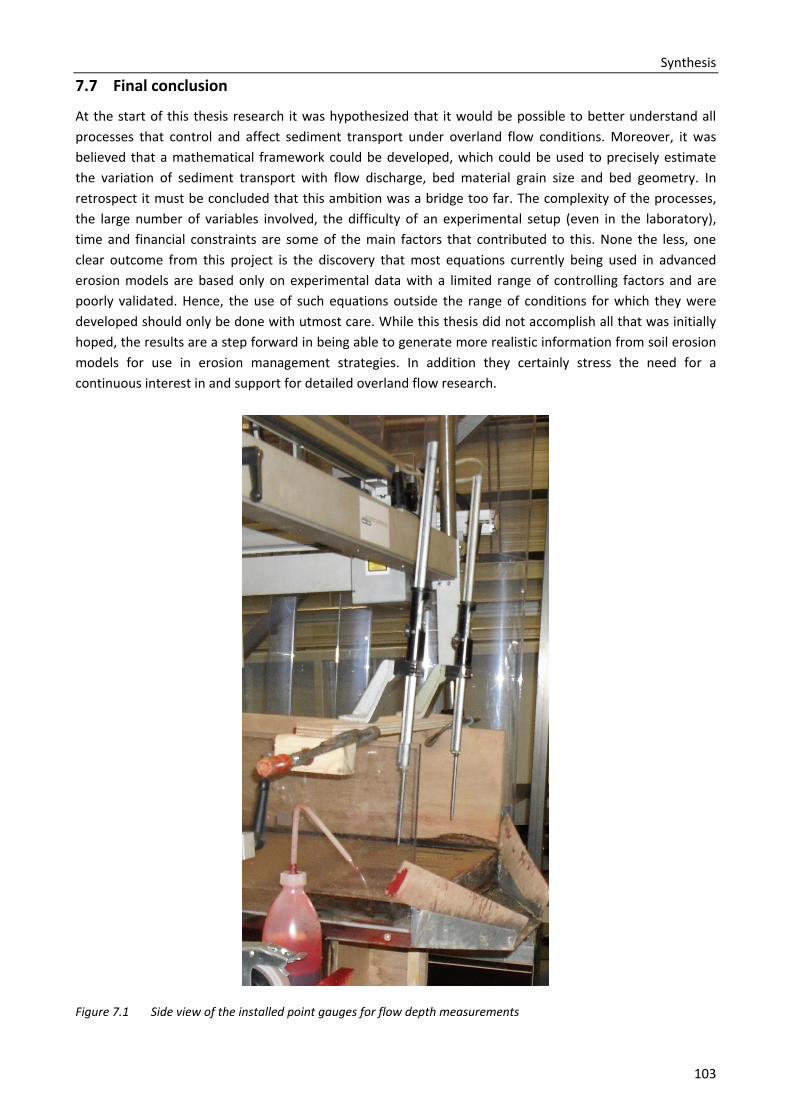
Synthesis
103
7.7 Final conclusion
At the start of this thesis research it was hypothesized that it would be possible to better understand all processes that control and affect sediment transport under overland flow conditions. Moreover, it was believed that a mathematical framework could be developed, which could be used to precisely estimate the variation of sediment transport with flow discharge, bed material grain size and bed geometry. In retrospect it must be concluded that this ambition was a bridge too far. The complexity of the processes, the large number of variables involved, the difficulty of an experimental setup (even in the laboratory), time and financial constraints are some of the main factors that contributed to this. None the less, one clear outcome from this project is the discovery that most equations currently being used in advanced erosion models are based only on experimental data with a limited range of controlling factors and are poorly validated. Hence, the use of such equations outside the range of conditions for which they were developed should only be done with utmost care. While this thesis did not accomplish all that was initially hoped, the results are a step forward in being able to generate more realistic information from soil erosion models for use in erosion management strategies. In addition they certainly stress the need for a continuous interest in and support for detailed overland flow research.
Figure 7.1 Side view of the installed point gauges for flow depth measurements

105
References Abrahams AD, Parsons AJ, Luk SH. 1986. Field measurement of the velocity of overland flow using dye tracing. Earth
Surface Processes and Landforms 11: 653–657. Abrahams AD, Atkinson JF. 1993. Relation between grain velocity and sediment concentration in overland flow. Water
Resources Research 29: 3021 – 3028. Abrahams AD, Parsons AJ. 1994. Hydraulics of interrill overland flow on stone-covered desert surfaces. Catena 23:
111-140. Abrahams AD, Li G, Parsons AJ. 1996. Rill hydraulics on a semiarid hillslope, Southern Arizona. Earth Surface Processes
and Landforms 21(1): 35 – 47. Abrahams AD, Li G. 1998. Effect of saltating sediment on flow resistance and bed roughness in overland flow. Earth
Surface Processes and Landforms 23: 953 – 960. Abrahams AD, Gao P, Aebly FA. 2000. Relation of sediment transport capacity to stone-cover and size in rain impacted
interrill flow. Earth Surface Processes and Landforms 25(5): 497 – 504. Abrahams AD, Li G, Krishnan C, Atkinson JF. 2001. A sediment transport equation for interrill overland flow on rough
surfaces. Earth Surface Processes and Landforms 26(13): 1443 – 1459. Acharya G, Cochrane TA, Davies T, Bowman E. 2009. The influence of shallow landslides on sediment supply: A flume-
based investigation using sandy soil. Engineering Geology 109(3-4): 161–169. Ahmadi SH, Amin S, Keshavarzi AR, Mirzamostafa N. 2006. Simulating watershed outlet sediment concentration using
the ANSWERS model by applying two sediment transport capacity equations. Biosystem Engineering 94(4): 615 – 626.
Ali KF, De Boer DH. 2007. Spatial patterns and variation of suspended sediment yield in the upper Indus river basin, Northern Pakistan. Journal of Hydrology 334: 368 – 387.
Ali M, Ahmad Z, Maqsood R, Siddique M. 2006. Performance of sediment transport functions for reservoir sediment simulation of mangla and tarbela reservoirs. Proceedings of the 8th International Summer Symposium, Japan Society of Civil Engineers, Nagoya, Japan. 87 – 90.
Ali M, Sterk G, Seeger M, Boersema M, Piet P. 2011a. Effect of hydraulic parameters on sediment transport capacity under overland flow conditions. Hydrology and Earth System Sciences Discussions 8: 6939 - 6965.
Ali M, Sterk G, Seeger M, Stroosnijder L. 2011b. Effect of discharge and grain size on mean flow velocity under overland flow conditions. Earth Surface Processes and Landforms. (in-review)
Allen JRL. 1994. Fundamental properties of fluids and their relation to sediment transport processes. In: Pye K. (Ed.) Sediment Transport and Depositional Processes. Oxford: Blackwell Scientific Publications, UK, 25 – 60.
Alonso CV, Neibling WH, Foster GR. 1981. Estimating sediment transport capacity in watershed modelling. Transaction of the American Society of Agricultural Engineers 24: 1211-1226.
Ayala JE, Martinez-Austria P, Menendez JR, Segura FA. 2000. Fixed bed forms laboratory channel flow analysis. Ingenieria Hidraulica En Mexico 15(2): 75–84.
Aziz NM, Scott DE. 1989. Experiments on sediment transport on shallow flows in high gradient channels. Journal of Hydrological Sciences 34: 465 – 479.
Bagarello V, Ferro V. 2004. Plot-scale measurement of soil erosion at the experimental area of Sparacia (Southern Italy). Hydrological Processes 18: 141 – 157.
Bagnold RA. 1956. The flow of cohesionless grains in fluids. Philosophical Transactions of the Royal Society of London A 249(964): 235 – 297.
Bagnold RA. 1966. An approach to the sediment transport problem from general physics. United States Geological Survey Professional Paper: 422-I.
Bagnold RA. 1980. An empirical correlation of bedload transport rates in flumes and natural rivers. Proceedings of the Royal Society of London A 372: 453–473.
Barrow CJ. 1991. Land Degradation. Cambridge University Press, Cambridge. Beasley DB, Huggins LF. 1982. ANSWERS user’s manual. Department of agricultural engineering, Purdue University,
West Lafayette, IN, 1982. Bergsma E. 1974. Soil erosion sequences on aerial photographs. ITC Journal 3: 342-376. Beven KJ. 2001. Rainfall-Runoff Modelling; The Primer. Wiley, Chichester, UK.
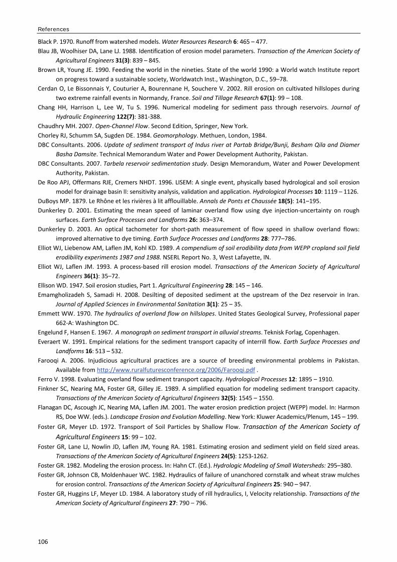
References
106
Black P. 1970. Runoff from watershed models. Water Resources Research 6: 465 – 477. Blau JB, Woolhiser DA, Lane LJ. 1988. Identification of erosion model parameters. Transaction of the American Society of
Agricultural Engineers 31(3): 839 – 845. Brown LR, Young JE. 1990. Feeding the world in the nineties. State of the world 1990: a World watch Institute report
on progress toward a sustainable society, Worldwatch Inst., Washington, D.C., 59–78. Cerdan O, Le Bissonnais Y, Couturier A, Bourennane H, Souchere V. 2002. Rill erosion on cultivated hillslopes during
two extreme rainfall events in Normandy, France. Soil and Tillage Research 67(1): 99 – 108. Chang HH, Harrison L, Lee W, Tu S. 1996. Numerical modeling for sediment pass through reservoirs. Journal of
Hydraulic Engineering 122(7): 381-388. Chaudhry MH. 2007. Open-Channel Flow. Second Edition, Springer, New York. Chorley RJ, Schumm SA, Sugden DE. 1984. Geomorphology. Methuen, London, 1984. DBC Consultants. 2006. Update of sediment transport of Indus river at Partab Bridge/Bunji, Besham Qila and Diamer
Basha Damsite. Technical Memorandum Water and Power Development Authority, Pakistan. DBC Consultants. 2007. Tarbela reservoir sedimentation study. Design Memorandum, Water and Power Development
Authority, Pakistan. De Roo APJ, Offermans RJE, Cremers NHDT. 1996. LISEM: A single event, physically based hydrological and soil erosion
model for drainage basin II: sensitivity analysis, validation and application. Hydrological Processes 10: 1119 – 1126. DuBoys MP. 1879. Le Rhône et les rivières à lit afflouillable. Annals de Ponts et Chaussée 18(5): 141–195. Dunkerley D. 2001. Estimating the mean speed of laminar overland flow using dye injection-uncertainty on rough
surfaces. Earth Surface Processes and Landforms 26: 363–374. Dunkerley D. 2003. An optical tachometer for short-path measurement of flow speed in shallow overland flows:
improved alternative to dye timing. Earth Surface Processes and Landforms 28: 777–786. Elliot WJ, Liebenow AM, Laflen JM, Kohl KD. 1989. A compendium of soil erodibility data from WEPP cropland soil field
erodibility experiments 1987 and 1988. NSERL Report No. 3, West Lafayette, IN. Elliot WJ, Laflen JM. 1993. A process-based rill erosion model. Transactions of the American Society of Agricultural
Engineers 36(1): 35–72. Ellison WD. 1947. Soil erosion studies, Part 1. Agricultural Engineering 28: 145 – 146. Emamgholizadeh S, Samadi H. 2008. Desilting of deposited sediment at the upstream of the Dez reservoir in Iran.
Journal of Applied Sciences in Environmental Sanitation 3(1): 25 – 35. Emmett WW. 1970. The hydraulics of overland flow on hillslopes. United States Geological Survey, Professional paper
662-A: Washington DC. Engelund F, Hansen E. 1967. A monograph on sediment transport in alluvial streams. Teknisk Forlag, Copenhagen. Everaert W. 1991. Empirical relations for the sediment transport capacity of interrill flow. Earth Surface Processes and
Landforms 16: 513 – 532. Farooqi A. 2006. Injudicious agricultural practices are a source of breeding environmental problems in Pakistan.
Available from,http://www.ruralfuturesconference.org/2006/Farooqi.pdf . Ferro V. 1998. Evaluating overland flow sediment transport capacity. Hydrological Processes 12: 1895 – 1910. Finkner SC, Nearing MA, Foster GR, Gilley JE. 1989. A simplified equation for modeling sediment transport capacity.
Transactions of the American Society of Agricultural Engineers 32(5): 1545 – 1550. Flanagan DC, Ascough JC, Nearing MA, Laflen JM. 2001. The water erosion prediction project (WEPP) model. In: Harmon
RS, Doe WW. (eds.). Landscape Erosion and Evolution Modelling. New York: Kluwer Academics/Plenum, 145 – 199. Foster GR, Meyer LD. 1972. Transport of Soil Particles by Shallow Flow. Transaction of the American Society of
Agricultural Engineers 15: 99 – 102. Foster GR, Lane LJ, Nowlin JD, Laflen JM, Young RA. 1981. Estimating erosion and sediment yield on field sized areas.
Transactions of the American Society of Agricultural Engineers 24(5): 1253-1262. Foster GR. 1982. Modeling the erosion process. In: Hahn CT. (Ed.). Hydrologic Modeling of Small Watersheds: 295–380. Foster GR, Johnson CB, Moldenhauer WC. 1982. Hydraulics of failure of unanchored cornstalk and wheat straw mulches
for erosion control. Transactions of the American Society of Agricultural Engineers 25: 940 – 947. Foster GR, Huggins LF, Meyer LD. 1984. A laboratory study of rill hydraulics, I, Velocity relationship. Transactions of the
American Society of Agricultural Engineers 27: 790 – 796.
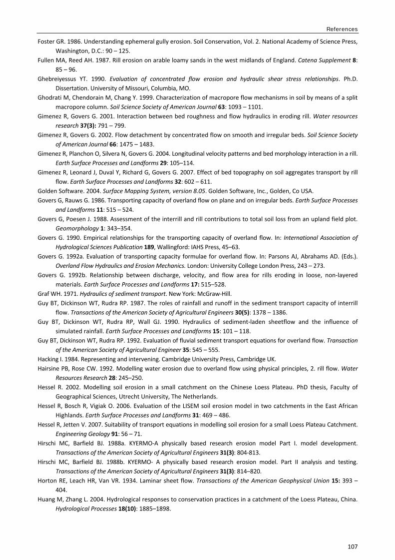
References
107
Foster GR. 1986. Understanding ephemeral gully erosion. Soil Conservation, Vol. 2. National Academy of Science Press, Washington, D.C.: 90 – 125.
Fullen MA, Reed AH. 1987. Rill erosion on arable loamy sands in the west midlands of England. Catena Supplement 8: 85 – 96.
Ghebreiyessus YT. 1990. Evaluation of concentrated flow erosion and hydraulic shear stress relationships. Ph.D. Dissertation. University of Missouri, Columbia, MO.
Ghodrati M, Chendorain M, Chang Y. 1999. Characterization of macropore flow mechanisms in soil by means of a split macropore column. Soil Science Society of American Journal 63: 1093 – 1101.
Gimenez R, Govers G. 2001. Interaction between bed roughness and flow hydraulics in eroding rill. Water resources research 37(3): 791 – 799.
Gimenez R, Govers G. 2002. Flow detachment by concentrated flow on smooth and irregular beds. Soil Science Society of American Journal 66: 1475 – 1483.
Gimenez R, Planchon O, Silvera N, Govers G. 2004. Longitudinal velocity patterns and bed morphology interaction in a rill. Earth Surface Processes and Landforms 29: 105–114.
Gimenez R, Leonard J, Duval Y, Richard G, Govers G. 2007. Effect of bed topography on soil aggregates transport by rill flow. Earth Surface Processes and Landforms 32: 602 – 611.
Golden Software. 2004. Surface Mapping System, version 8.05. Golden Software, Inc., Golden, Co USA. Govers G, Rauws G. 1986. Transporting capacity of overland flow on plane and on irregular beds. Earth Surface Processes
and Landforms 11: 515 – 524. Govers G, Poesen J. 1988. Assessment of the interrill and rill contributions to total soil loss from an upland field plot.
Geomorphology 1: 343–354. Govers G. 1990. Empirical relationships for the transporting capacity of overland flow. In: International Association of
Hydrological Sciences Publication 189, Wallingford: IAHS Press, 45–63. Govers G. 1992a. Evaluation of transporting capacity formulae for overland flow. In: Parsons AJ, Abrahams AD. (Eds.).
Overland Flow Hydraulics and Erosion Mechanics. London: University College London Press, 243 – 273. Govers G. 1992b. Relationship between discharge, velocity, and flow area for rills eroding in loose, non-layered
materials. Earth Surface Processes and Landforms 17: 515–528. Graf WH. 1971. Hydraulics of sediment transport. New York: McGraw-Hill. Guy BT, Dickinson WT, Rudra RP. 1987. The roles of rainfall and runoff in the sediment transport capacity of interrill
flow. Transactions of the American Society of Agricultural Engineers 30(5): 1378 – 1386. Guy BT, Dickinson WT, Rudra RP, Wall GJ. 1990. Hydraulics of sediment-laden sheetflow and the influence of
simulated rainfall. Earth Surface Processes and Landforms 15: 101 – 118. Guy BT, Dickinson WT, Rudra RP. 1992. Evaluation of fluvial sediment transport equations for overland flow. Transaction
of the American Society of Agricultural Engineer 35: 545 – 555. Hacking I. 1984. Representing and intervening. Cambridge University Press, Cambridge UK. Hairsine PB, Rose CW. 1992. Modelling water erosion due to overland flow using physical principles, 2. rill flow. Water
Resources Research 28: 245–250. Hessel R. 2002. Modelling soil erosion in a small catchment on the Chinese Loess Plateau. PhD thesis, Faculty of
Geographical Sciences, Utrecht University, The Netherlands. Hessel R, Bosch R, Vigiak O. 2006. Evaluation of the LISEM soil erosion model in two catchments in the East African
Highlands. Earth Surface Processes and Landforms 31: 469 – 486. Hessel R, Jetten V. 2007. Suitability of transport equations in modelling soil erosion for a small Loess Plateau Catchment.
Engineering Geology 91: 56 – 71. Hirschi MC, Barfield BJ. 1988a. KYERMO-A physically based research erosion model Part I. model development.
Transactions of the American Society of Agricultural Engineers 31(3): 804-813. Hirschi MC, Barfield BJ. 1988b. KYERMO- A physically based research erosion model. Part II analysis and testing.
Transactions of the American Society of Agricultural Engineers 31(3): 814–820. Horton RE, Leach HR, Van VR. 1934. Laminar sheet flow. Transactions of the American Geophysical Union 15: 393 –
404. Huang M, Zhang L. 2004. Hydrological responses to conservation practices in a catchment of the Loess Plateau, China.
Hydrological Processes 18(10): 1885–1898.
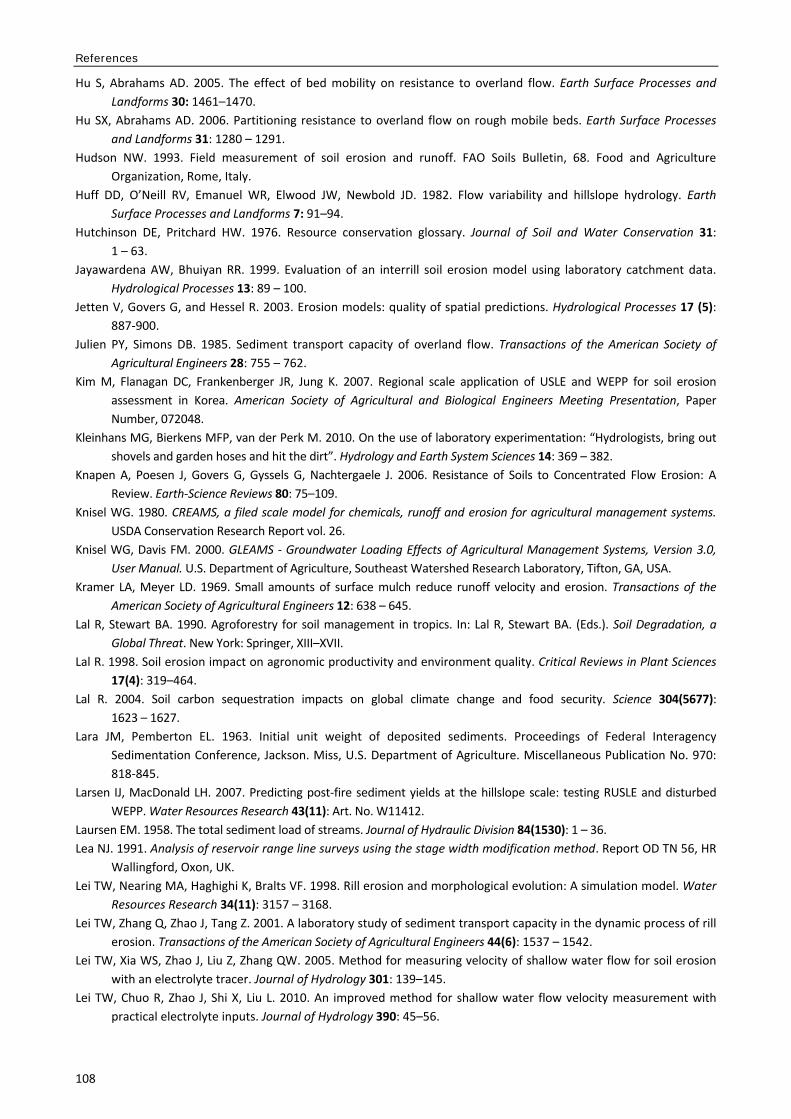
References
108
Hu S, Abrahams AD. 2005. The effect of bed mobility on resistance to overland flow. Earth Surface Processes and Landforms 30: 1461–1470.
Hu SX, Abrahams AD. 2006. Partitioning resistance to overland flow on rough mobile beds. Earth Surface Processes and Landforms 31: 1280 – 1291.
Hudson NW. 1993. Field measurement of soil erosion and runoff. FAO Soils Bulletin, 68. Food and Agriculture Organization, Rome, Italy.
Huff DD, O’Neill RV, Emanuel WR, Elwood JW, Newbold JD. 1982. Flow variability and hillslope hydrology. Earth Surface Processes and Landforms 7: 91–94.
Hutchinson DE, Pritchard HW. 1976. Resource conservation glossary. Journal of Soil and Water Conservation 31: 1 – 63.
Jayawardena AW, Bhuiyan RR. 1999. Evaluation of an interrill soil erosion model using laboratory catchment data. Hydrological Processes 13: 89 – 100.
Jetten V, Govers G, and Hessel R. 2003. Erosion models: quality of spatial predictions. Hydrological Processes 17 (5): 887-900.
Julien PY, Simons DB. 1985. Sediment transport capacity of overland flow. Transactions of the American Society of Agricultural Engineers 28: 755 – 762.
Kim M, Flanagan DC, Frankenberger JR, Jung K. 2007. Regional scale application of USLE and WEPP for soil erosion assessment in Korea. American Society of Agricultural and Biological Engineers Meeting Presentation, Paper Number, 072048.
Kleinhans MG, Bierkens MFP, van der Perk M. 2010. On the use of laboratory experimentation: “Hydrologists, bring out shovels and garden hoses and hit the dirt”. Hydrology and Earth System Sciences 14: 369 – 382.
Knapen A, Poesen J, Govers G, Gyssels G, Nachtergaele J. 2006. Resistance of Soils to Concentrated Flow Erosion: A Review. Earth-Science Reviews 80: 75–109.
Knisel WG. 1980. CREAMS, a filed scale model for chemicals, runoff and erosion for agricultural management systems. USDA Conservation Research Report vol. 26.
Knisel WG, Davis FM. 2000. GLEAMS - Groundwater Loading Effects of Agricultural Management Systems, Version 3.0, User Manual. U.S. Department of Agriculture, Southeast Watershed Research Laboratory, Tifton, GA, USA.
Kramer LA, Meyer LD. 1969. Small amounts of surface mulch reduce runoff velocity and erosion. Transactions of the American Society of Agricultural Engineers 12: 638 – 645.
Lal R, Stewart BA. 1990. Agroforestry for soil management in tropics. In: Lal R, Stewart BA. (Eds.). Soil Degradation, a Global Threat. New York: Springer, XIII–XVII.
Lal R. 1998. Soil erosion impact on agronomic productivity and environment quality. Critical Reviews in Plant Sciences 17(4): 319–464.
Lal R. 2004. Soil carbon sequestration impacts on global climate change and food security. Science 304(5677): 1623 – 1627.
Lara JM, Pemberton EL. 1963. Initial unit weight of deposited sediments. Proceedings of Federal Interagency Sedimentation Conference, Jackson. Miss, U.S. Department of Agriculture. Miscellaneous Publication No. 970: 818-845.
Larsen IJ, MacDonald LH. 2007. Predicting post-fire sediment yields at the hillslope scale: testing RUSLE and disturbed WEPP. Water Resources Research 43(11): Art. No. W11412.
Laursen EM. 1958. The total sediment load of streams. Journal of Hydraulic Division 84(1530): 1 – 36. Lea NJ. 1991. Analysis of reservoir range line surveys using the stage width modification method. Report OD TN 56, HR
Wallingford, Oxon, UK. Lei TW, Nearing MA, Haghighi K, Bralts VF. 1998. Rill erosion and morphological evolution: A simulation model. Water
Resources Research 34(11): 3157 – 3168. Lei TW, Zhang Q, Zhao J, Tang Z. 2001. A laboratory study of sediment transport capacity in the dynamic process of rill
erosion. Transactions of the American Society of Agricultural Engineers 44(6): 1537 – 1542. Lei TW, Xia WS, Zhao J, Liu Z, Zhang QW. 2005. Method for measuring velocity of shallow water flow for soil erosion
with an electrolyte tracer. Journal of Hydrology 301: 139–145. Lei TW, Chuo R, Zhao J, Shi X, Liu L. 2010. An improved method for shallow water flow velocity measurement with
practical electrolyte inputs. Journal of Hydrology 390: 45–56.
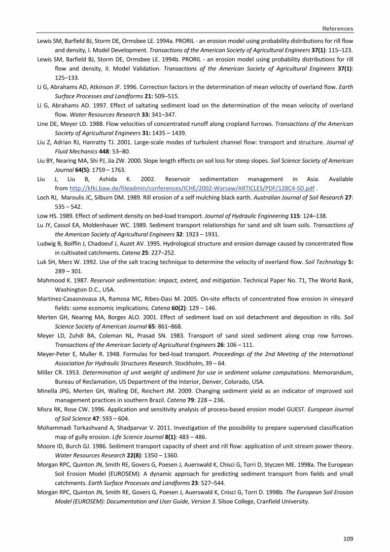
References
109
Lewis SM, Barfield BJ, Storm DE, Ormsbee LE. 1994a. PRORIL - an erosion model using probability distributions for rill flow and density, I. Model Development. Transactions of the American Society of Agricultural Engineers 37(1): 115–123.
Lewis SM, Barfield BJ, Storm DE, Ormsbee LE. 1994b. PRORIL - an erosion model using probability distributions for rill flow and density, II. Model Validation. Transactions of the American Society of Agricultural Engineers 37(1): 125–133.
Li G, Abrahams AD, Atkinson JF. 1996. Correction factors in the determination of mean velocity of overland flow. Earth Surface Processes and Landforms 21: 509–515.
Li G, Abrahams AD. 1997. Effect of saltating sediment load on the determination of the mean velocity of overland flow. Water Resources Research 33: 341–347.
Line DE, Meyer LD. 1988. Flow velocities of concentrated runoff along cropland furrows. Transactions of the American Society of Agricultural Engineers 31: 1435 – 1439.
Liu Z, Adrian RJ, Hanratty TJ. 2001. Large-scale modes of turbulent channel flow: transport and structure. Journal of Fluid Mechanics 448: 53–80.
Liu BY, Nearing MA, Shi PJ, Jia ZW. 2000. Slope length effects on soil loss for steep slopes. Soil Science Society of American Journal 64(5): 1759 – 1763.
Liu J, Liu B, Ashida K. 2002. Reservoir sedimentation management in Asia. Available from,http://kfki.baw.de/fileadmin/conferences/ICHE/2002-Warsaw/ARTICLES/PDF/128C4-SD.pdf .
Loch RJ, Maroulis JC, Silburn DM. 1989. Rill erosion of a self mulching black earth. Australian Journal of Soil Research 27: 535 – 542.
Low HS. 1989. Effect of sediment density on bed-load transport. Journal of Hydraulic Engineering 115: 124–138. Lu JY, Cassol EA, Moldenhauer WC. 1989. Sediment transport relationships for sand and silt loam soils. Transactions of
the American Society of Agricultural Engineers 32: 1923 – 1931. Ludwig B, Boiffin J, Chadoeuf J, Auzet AV. 1995. Hydrological structure and erosion damage caused by concentrated flow
in cultivated catchments. Catena 25: 227–252. Luk SH, Merz W. 1992. Use of the salt tracing technique to determine the velocity of overland flow. Soil Technology 5:
289 – 301. Mahmood K. 1987. Reservoir sedimentation: impact, extent, and mitigation. Technical Paper No. 71, The World Bank,
Washington D.C., USA. Martinez-Casasnovasa JA, Ramosa MC, Ribes-Dasi M. 2005. On-site effects of concentrated flow erosion in vineyard
fields: some economic implications. Catena 60(2): 129 – 146. Merten GH, Nearing MA, Borges ALO. 2001. Effect of sediment load on soil detachment and deposition in rills. Soil
Science Society of American Journal 65: 861–868. Meyer LD, Zuhdi BA, Coleman NL, Prasad SN. 1983. Transport of sand sized sediment along crop row furrows.
Transactions of the American Society of Agricultural Engineers 26: 106 – 111. Meyer-Peter E, Muller R. 1948. Formulas for bed-load transport. Proceedings of the 2nd Meeting of the International
Association for Hydraulic Structures Research. Stockholm, 39 – 64. Miller CR. 1953. Determination of unit weight of sediment for use in sediment volume computations. Memorandum,
Bureau of Reclamation, US Department of the Interior, Denver, Colorado, USA. Minella JPG, Merten GH, Walling DE, Reichert JM. 2009. Changing sediment yield as an indicator of improved soil
management practices in southern Brazil. Catena 79: 228 – 236. Misra RK, Rose CW. 1996. Application and sensitivity analysis of process-based erosion model GUEST. European Journal
of Soil Science 47: 593 – 604. Mohammadi Torkashvand A, Shadparvar V. 2011. Investigation of the possibility to prepare supervised classification
map of gully erosion. Life Science Journal 8(1): 483 – 486. Moore ID, Burch GJ. 1986. Sediment transport capacity of sheet and rill flow: application of unit stream power theory.
Water Resources Research 22(8): 1350 – 1360. Morgan RPC, Quinton JN, Smith RE, Govers G, Poesen J, Auerswald K, Chisci G, Torri D, Styczen ME. 1998a. The European
Soil Erosion Model (EUROSEM): A dynamic approach for predicting sediment transport from fields and small catchments. Earth Surface Processes and Landforms 23: 527–544.
Morgan RPC, Quinton JN, Smith RE, Govers G, Poesen J, Auerswald K, Cnisci G, Torri D. 1998b. The European Soil Erosion Model (EUROSEM): Documentation and User Guide, Version 3. Silsoe College, Cranfield University.
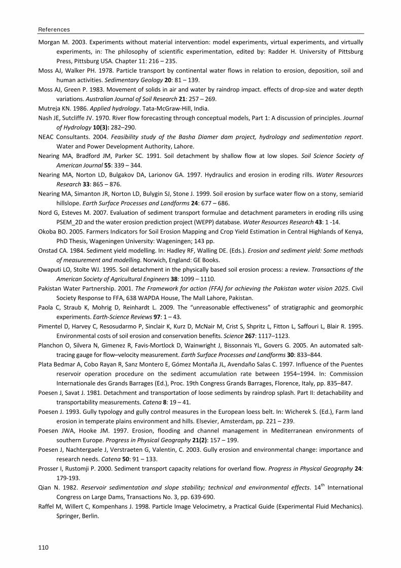
References
110
Morgan M. 2003. Experiments without material intervention: model experiments, virtual experiments, and virtually experiments, in: The philosophy of scientific experimentation, edited by: Radder H. University of Pittsburg Press, Pittsburg USA. Chapter 11: 216 – 235.
Moss AJ, Walker PH. 1978. Particle transport by continental water flows in relation to erosion, deposition, soil and human activities. Sedimentary Geology 20: 81 – 139.
Moss AJ, Green P. 1983. Movement of solids in air and water by raindrop impact. effects of drop-size and water depth variations. Australian Journal of Soil Research 21: 257 – 269.
Mutreja KN. 1986. Applied hydrology. Tata-McGraw-Hill, India. Nash JE, Sutcliffe JV. 1970. River flow forecasting through conceptual models, Part 1: A discussion of principles. Journal
of Hydrology 10(3): 282–290. NEAC Consultants. 2004. Feasibility study of the Basha Diamer dam project, hydrology and sedimentation report.
Water and Power Development Authority, Lahore. Nearing MA, Bradford JM, Parker SC. 1991. Soil detachment by shallow flow at low slopes. Soil Science Society of
American Journal 55: 339 – 344. Nearing MA, Norton LD, Bulgakov DA, Larionov GA. 1997. Hydraulics and erosion in eroding rills. Water Resources
Research 33: 865 – 876. Nearing MA, Simanton JR, Norton LD, Bulygin SJ, Stone J. 1999. Soil erosion by surface water flow on a stony, semiarid
hillslope. Earth Surface Processes and Landforms 24: 677 – 686. Nord G, Esteves M. 2007. Evaluation of sediment transport formulae and detachment parameters in eroding rills using
PSEM_2D and the water erosion prediction project (WEPP) database. Water Resources Research 43: 1 -14. Okoba BO. 2005. Farmers Indicators for Soil Erosion Mapping and Crop Yield Estimation in Central Highlands of Kenya,
PhD Thesis, Wageningen University: Wageningen; 143 pp. Onstad CA. 1984. Sediment yield modelling. In: Hadley RF, Walling DE. (Eds.). Erosion and sediment yield: Some methods
of measurement and modelling. Norwich, England: GE Books. Owaputi LO, Stolte WJ. 1995. Soil detachment in the physically based soil erosion process: a review. Transactions of the
American Society of Agricultural Engineers 38: 1099 – 1110. Pakistan Water Partnership. 2001. The Framework for action (FFA) for achieving the Pakistan water vision 2025. Civil
Society Response to FFA, 638 WAPDA House, The Mall Lahore, Pakistan. Paola C, Straub K, Mohrig D, Reinhardt L. 2009. The “unreasonable effectiveness” of stratigraphic and geomorphic
experiments. Earth-Science Reviews 97: 1 – 43. Pimentel D, Harvey C, Resosudarmo P, Sinclair K, Kurz D, McNair M, Crist S, Shpritz L, Fitton L, Saffouri L, Blair R. 1995.
Environmental costs of soil erosion and conservation benefits. Science 267: 1117–1123. Planchon O, Silvera N, Gimenez R, Favis-Mortlock D, Wainwright J, Bissonnais YL, Govers G. 2005. An automated salt-
tracing gauge for flow–velocity measurement. Earth Surface Processes and Landforms 30: 833–844. Plata Bedmar A, Cobo Rayan R, Sanz Montero E, Gómez Montaña JL, Avendaño Salas C. 1997. Influence of the Puentes
reservoir operation procedure on the sediment accumulation rate between 1954–1994. In: Commission Internationale des Grands Barrages (Ed.), Proc. 19th Congress Grands Barrages, Florence, Italy, pp. 835–847.
Poesen J, Savat J. 1981. Detachment and transportation of loose sediments by raindrop splash. Part II: detachability and transportability measurements. Catena 8: 19 – 41.
Poesen J. 1993. Gully typology and gully control measures in the European loess belt. In: Wicherek S. (Ed.), Farm land erosion in temperate plains environment and hills. Elsevier, Amsterdam, pp. 221 – 239.
Poesen JWA, Hooke JM. 1997. Erosion, flooding and channel management in Mediterranean environments of southern Europe. Progress in Physical Geography 21(2): 157 – 199.
Poesen J, Nachtergaele J, Verstraeten G, Valentin, C. 2003. Gully erosion and environmental change: importance and research needs. Catena 50: 91 – 133.
Prosser I, Rustomji P. 2000. Sediment transport capacity relations for overland flow. Progress in Physical Geography 24: 179-193.
Qian N. 1982. Reservoir sedimentation and slope stability; technical and environmental effects. 14th International Congress on Large Dams, Transactions No. 3, pp. 639-690.
Raffel M, Willert C, Kompenhans J. 1998. Particle Image Velocimetry, a Practical Guide (Experimental Fluid Mechanics). Springer, Berlin.
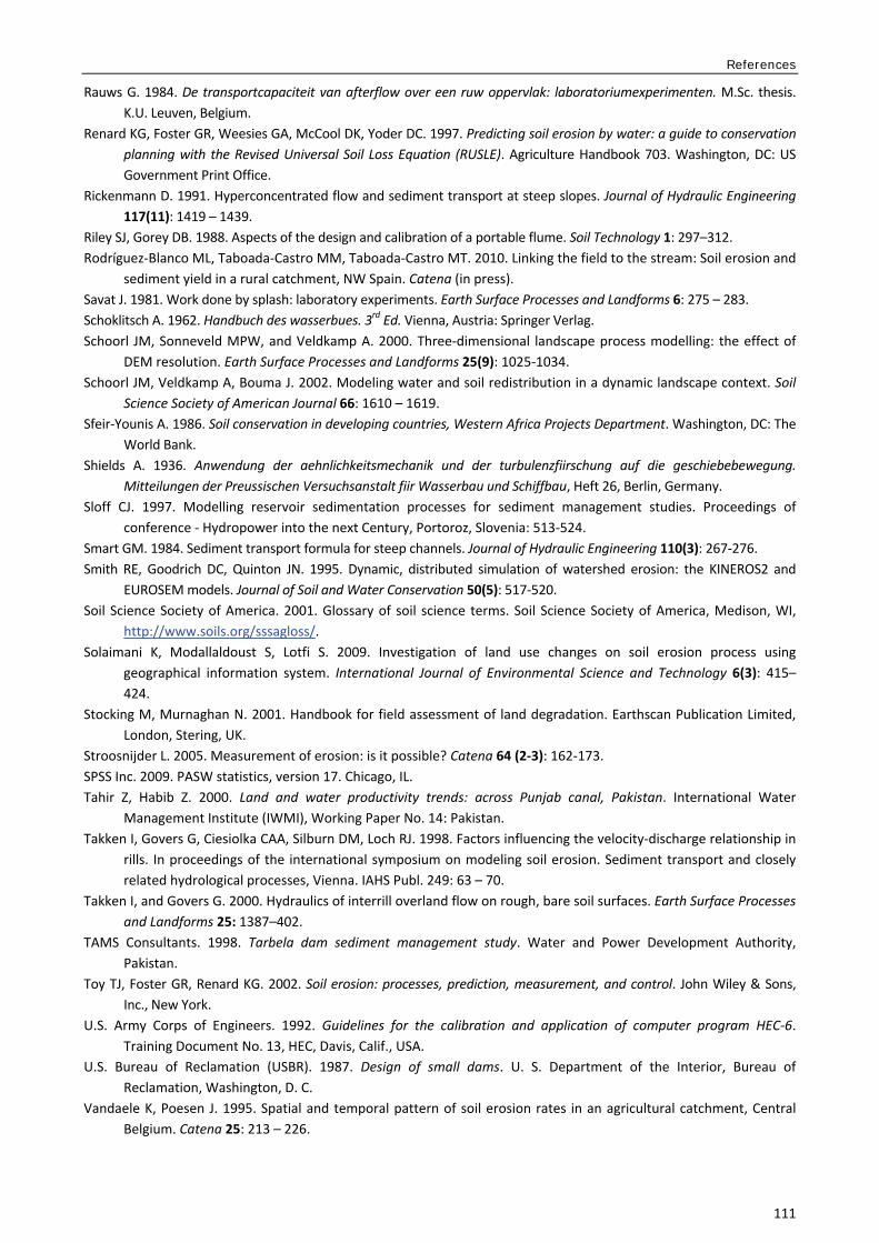
References
111
Rauws G. 1984. De transportcapaciteit van afterflow over een ruw oppervlak: laboratoriumexperimenten. M.Sc. thesis. K.U. Leuven, Belgium.
Renard KG, Foster GR, Weesies GA, McCool DK, Yoder DC. 1997. Predicting soil erosion by water: a guide to conservation planning with the Revised Universal Soil Loss Equation (RUSLE). Agriculture Handbook 703. Washington, DC: US Government Print Office.
Rickenmann D. 1991. Hyperconcentrated flow and sediment transport at steep slopes. Journal of Hydraulic Engineering 117(11): 1419 – 1439.
Riley SJ, Gorey DB. 1988. Aspects of the design and calibration of a portable flume. Soil Technology 1: 297–312. Rodríguez-Blanco ML, Taboada-Castro MM, Taboada-Castro MT. 2010. Linking the field to the stream: Soil erosion and
sediment yield in a rural catchment, NW Spain. Catena (in press). Savat J. 1981. Work done by splash: laboratory experiments. Earth Surface Processes and Landforms 6: 275 – 283. Schoklitsch A. 1962. Handbuch des wasserbues. 3rd Ed. Vienna, Austria: Springer Verlag. Schoorl JM, Sonneveld MPW, and Veldkamp A. 2000. Three-dimensional landscape process modelling: the effect of
DEM resolution. Earth Surface Processes and Landforms 25(9): 1025-1034. Schoorl JM, Veldkamp A, Bouma J. 2002. Modeling water and soil redistribution in a dynamic landscape context. Soil
Science Society of American Journal 66: 1610 – 1619. Sfeir-Younis A. 1986. Soil conservation in developing countries, Western Africa Projects Department. Washington, DC: The
World Bank. Shields A. 1936. Anwendung der aehnlichkeitsmechanik und der turbulenzfiirschung auf die geschiebebewegung.
Mitteilungen der Preussischen Versuchsanstalt fiir Wasserbau und Schiffbau, Heft 26, Berlin, Germany. Sloff CJ. 1997. Modelling reservoir sedimentation processes for sediment management studies. Proceedings of
conference - Hydropower into the next Century, Portoroz, Slovenia: 513-524. Smart GM. 1984. Sediment transport formula for steep channels. Journal of Hydraulic Engineering 110(3): 267-276. Smith RE, Goodrich DC, Quinton JN. 1995. Dynamic, distributed simulation of watershed erosion: the KINEROS2 and
EUROSEM models. Journal of Soil and Water Conservation 50(5): 517-520. Soil Science Society of America. 2001. Glossary of soil science terms. Soil Science Society of America, Medison, WI,
http://www.soils.org/sssagloss/. Solaimani K, Modallaldoust S, Lotfi S. 2009. Investigation of land use changes on soil erosion process using
geographical information system. International Journal of Environmental Science and Technology 6(3): 415– 424.
Stocking M, Murnaghan N. 2001. Handbook for field assessment of land degradation. Earthscan Publication Limited, London, Stering, UK.
Stroosnijder L. 2005. Measurement of erosion: is it possible? Catena 64 (2-3): 162-173. SPSS Inc. 2009. PASW statistics, version 17. Chicago, IL. Tahir Z, Habib Z. 2000. Land and water productivity trends: across Punjab canal, Pakistan. International Water
Management Institute (IWMI), Working Paper No. 14: Pakistan. Takken I, Govers G, Ciesiolka CAA, Silburn DM, Loch RJ. 1998. Factors influencing the velocity-discharge relationship in
rills. In proceedings of the international symposium on modeling soil erosion. Sediment transport and closely related hydrological processes, Vienna. IAHS Publ. 249: 63 – 70.
Takken I, and Govers G. 2000. Hydraulics of interrill overland flow on rough, bare soil surfaces. Earth Surface Processes and Landforms 25: 1387–402.
TAMS Consultants. 1998. Tarbela dam sediment management study. Water and Power Development Authority, Pakistan.
Toy TJ, Foster GR, Renard KG. 2002. Soil erosion: processes, prediction, measurement, and control. John Wiley & Sons, Inc., New York.
U.S. Army Corps of Engineers. 1992. Guidelines for the calibration and application of computer program HEC-6. Training Document No. 13, HEC, Davis, Calif., USA.
U.S. Bureau of Reclamation (USBR). 1987. Design of small dams. U. S. Department of the Interior, Bureau of Reclamation, Washington, D. C.
Vandaele K, Poesen J. 1995. Spatial and temporal pattern of soil erosion rates in an agricultural catchment, Central Belgium. Catena 25: 213 – 226.
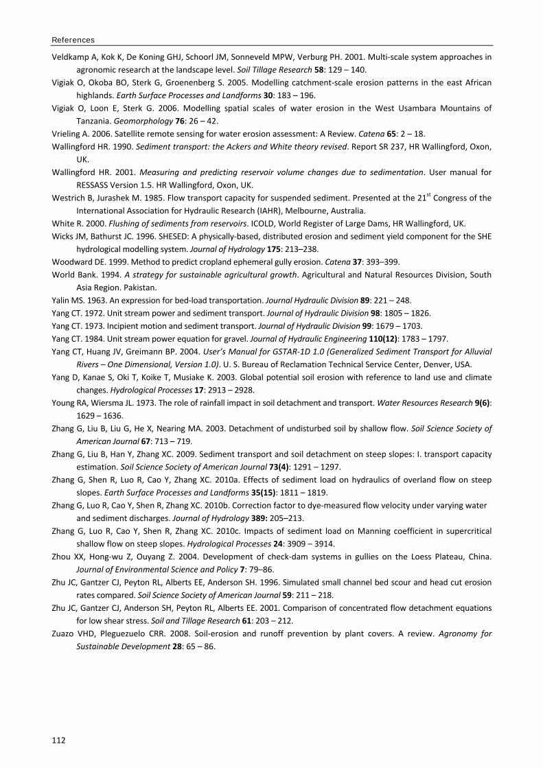
References
112
Veldkamp A, Kok K, De Koning GHJ, Schoorl JM, Sonneveld MPW, Verburg PH. 2001. Multi-scale system approaches in agronomic research at the landscape level. Soil Tillage Research 58: 129 – 140.
Vigiak O, Okoba BO, Sterk G, Groenenberg S. 2005. Modelling catchment-scale erosion patterns in the east African highlands. Earth Surface Processes and Landforms 30: 183 – 196.
Vigiak O, Loon E, Sterk G. 2006. Modelling spatial scales of water erosion in the West Usambara Mountains of Tanzania. Geomorphology 76: 26 – 42.
Vrieling A. 2006. Satellite remote sensing for water erosion assessment: A Review. Catena 65: 2 – 18. Wallingford HR. 1990. Sediment transport: the Ackers and White theory revised. Report SR 237, HR Wallingford, Oxon,
UK. Wallingford HR. 2001. Measuring and predicting reservoir volume changes due to sedimentation. User manual for
RESSASS Version 1.5. HR Wallingford, Oxon, UK. Westrich B, Jurashek M. 1985. Flow transport capacity for suspended sediment. Presented at the 21st Congress of the
International Association for Hydraulic Research (IAHR), Melbourne, Australia. White R. 2000. Flushing of sediments from reservoirs. ICOLD, World Register of Large Dams, HR Wallingford, UK. Wicks JM, Bathurst JC. 1996. SHESED: A physically-based, distributed erosion and sediment yield component for the SHE
hydrological modelling system. Journal of Hydrology 175: 213–238. Woodward DE. 1999. Method to predict cropland ephemeral gully erosion. Catena 37: 393–399. World Bank. 1994. A strategy for sustainable agricultural growth. Agricultural and Natural Resources Division, South
Asia Region. Pakistan. Yalin MS. 1963. An expression for bed-load transportation. Journal Hydraulic Division 89: 221 – 248. Yang CT. 1972. Unit stream power and sediment transport. Journal of Hydraulic Division 98: 1805 – 1826. Yang CT. 1973. Incipient motion and sediment transport. Journal of Hydraulic Division 99: 1679 – 1703. Yang CT. 1984. Unit stream power equation for gravel. Journal of Hydraulic Engineering 110(12): 1783 – 1797. Yang CT, Huang JV, Greimann BP. 2004. User’s Manual for GSTAR-1D 1.0 (Generalized Sediment Transport for Alluvial
Rivers – One Dimensional, Version 1.0). U. S. Bureau of Reclamation Technical Service Center, Denver, USA. Yang D, Kanae S, Oki T, Koike T, Musiake K. 2003. Global potential soil erosion with reference to land use and climate
changes. Hydrological Processes 17: 2913 – 2928. Young RA, Wiersma JL. 1973. The role of rainfall impact in soil detachment and transport. Water Resources Research 9(6):
1629 – 1636. Zhang G, Liu B, Liu G, He X, Nearing MA. 2003. Detachment of undisturbed soil by shallow flow. Soil Science Society of
American Journal 67: 713 – 719. Zhang G, Liu B, Han Y, Zhang XC. 2009. Sediment transport and soil detachment on steep slopes: I. transport capacity
estimation. Soil Science Society of American Journal 73(4): 1291 – 1297. Zhang G, Shen R, Luo R, Cao Y, Zhang XC. 2010a. Effects of sediment load on hydraulics of overland flow on steep
slopes. Earth Surface Processes and Landforms 35(15): 1811 – 1819. Zhang G, Luo R, Cao Y, Shen R, Zhang XC. 2010b. Correction factor to dye-measured flow velocity under varying water
and sediment discharges. Journal of Hydrology 389: 205–213. Zhang G, Luo R, Cao Y, Shen R, Zhang XC. 2010c. Impacts of sediment load on Manning coefficient in supercritical
shallow flow on steep slopes. Hydrological Processes 24: 3909 – 3914. Zhou XX, Hong-wu Z, Ouyang Z. 2004. Development of check-dam systems in gullies on the Loess Plateau, China.
Journal of Environmental Science and Policy 7: 79–86. Zhu JC, Gantzer CJ, Peyton RL, Alberts EE, Anderson SH. 1996. Simulated small channel bed scour and head cut erosion
rates compared. Soil Science Society of American Journal 59: 211 – 218. Zhu JC, Gantzer CJ, Anderson SH, Peyton RL, Alberts EE. 2001. Comparison of concentrated flow detachment equations
for low shear stress. Soil and Tillage Research 61: 203 – 212. Zuazo VHD, Pleguezuelo CRR. 2008. Soil-erosion and runoff prevention by plant covers. A review. Agronomy for
Sustainable Development 28: 65 – 86.

Summary

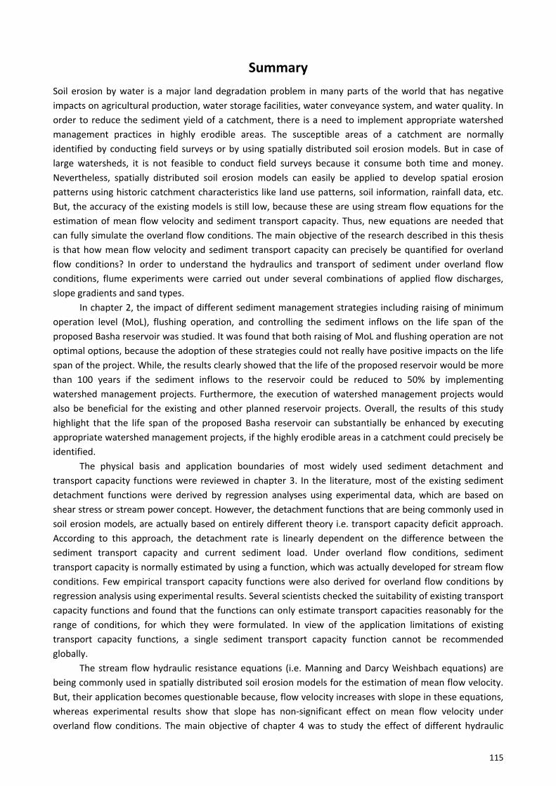
115
Summary Soil erosion by water is a major land degradation problem in many parts of the world that has negative impacts on agricultural production, water storage facilities, water conveyance system, and water quality. In order to reduce the sediment yield of a catchment, there is a need to implement appropriate watershed management practices in highly erodible areas. The susceptible areas of a catchment are normally identified by conducting field surveys or by using spatially distributed soil erosion models. But in case of large watersheds, it is not feasible to conduct field surveys because it consume both time and money. Nevertheless, spatially distributed soil erosion models can easily be applied to develop spatial erosion patterns using historic catchment characteristics like land use patterns, soil information, rainfall data, etc. But, the accuracy of the existing models is still low, because these are using stream flow equations for the estimation of mean flow velocity and sediment transport capacity. Thus, new equations are needed that can fully simulate the overland flow conditions. The main objective of the research described in this thesis is that how mean flow velocity and sediment transport capacity can precisely be quantified for overland flow conditions? In order to understand the hydraulics and transport of sediment under overland flow conditions, flume experiments were carried out under several combinations of applied flow discharges, slope gradients and sand types.
In chapter 2, the impact of different sediment management strategies including raising of minimum operation level (MoL), flushing operation, and controlling the sediment inflows on the life span of the proposed Basha reservoir was studied. It was found that both raising of MoL and flushing operation are not optimal options, because the adoption of these strategies could not really have positive impacts on the life span of the project. While, the results clearly showed that the life of the proposed reservoir would be more than 100 years if the sediment inflows to the reservoir could be reduced to 50% by implementing watershed management projects. Furthermore, the execution of watershed management projects would also be beneficial for the existing and other planned reservoir projects. Overall, the results of this study highlight that the life span of the proposed Basha reservoir can substantially be enhanced by executing appropriate watershed management projects, if the highly erodible areas in a catchment could precisely be identified.
The physical basis and application boundaries of most widely used sediment detachment and transport capacity functions were reviewed in chapter 3. In the literature, most of the existing sediment detachment functions were derived by regression analyses using experimental data, which are based on shear stress or stream power concept. However, the detachment functions that are being commonly used in soil erosion models, are actually based on entirely different theory i.e. transport capacity deficit approach. According to this approach, the detachment rate is linearly dependent on the difference between the sediment transport capacity and current sediment load. Under overland flow conditions, sediment transport capacity is normally estimated by using a function, which was actually developed for stream flow conditions. Few empirical transport capacity functions were also derived for overland flow conditions by regression analysis using experimental results. Several scientists checked the suitability of existing transport capacity functions and found that the functions can only estimate transport capacities reasonably for the range of conditions, for which they were formulated. In view of the application limitations of existing transport capacity functions, a single sediment transport capacity function cannot be recommended globally.
The stream flow hydraulic resistance equations (i.e. Manning and Darcy Weishbach equations) are being commonly used in spatially distributed soil erosion models for the estimation of mean flow velocity. But, their application becomes questionable because, flow velocity increases with slope in these equations, whereas experimental results show that slope has non-significant effect on mean flow velocity under overland flow conditions. The main objective of chapter 4 was to study the effect of different hydraulic
Summary
116
parameters (like flow discharge, slope gradient) and grain size on mean flow velocity under overland flow. The results of this study corroborate the findings of previous studies in way that the mean flow velocity is substantially affected by flow discharge, while slope gradient exhibited non-significant effect. Moreover, grain size also showed significant effect on mean flow velocity. The results showed that mean flow velocity decreases with the increase of grain size, because bed roughness increases with grain size. In view of the results of this study, a new empirical equation was proposed for the precise estimation of mean flow velocity.
In the literature, the influence of different hydraulic parameters (i.e. unit discharge, mean flow velocity, and slope gradient) on sediment transport capacity was mostly studied for non-erodible beds under overland flow conditions. The theoretical concepts derived from non-erodible beds are needed to be verified for erodible bed conditions. In chapter 5, the influence of these parameters on transport capacity was studied for erodible beds. It was concluded that the derived theoretical concepts from non-erodible beds do not completely portray the erodible bed conditions, because (i) roughness of erodible beds are significantly higher than non-erodible beds for the similar hydraulic and sediment conditions (ii) the available flow energy is utilised on bed irregularities, detachment and transport of sediment particles under erodible beds, whereas the available flow energy is preferentially consumed on transport of sediment for non-erodible beds. Therefore the application of transport capacity functions, derived for non-erodible beds, are become debatable when applied to a natural hillslope. Moreover in this study, the potential of four composite force predictors (i.e. shear stress, stream power, unit stream power and effective stream power) was also evaluated for the estimation of transport capacity. All the selected composite predictors showed strong relationships with transport capacity, except shear stress. Because part of the shear stress (i.e. form shear stress) is used for the detachment of sediment particles from soil matrix under erodible beds instead of transporting sediment particles. Among the selected predictors, preference has given to the unit stream power concept because, its relationship with transport capacity was found independent of grain size effect.
In chapter 6 of this thesis, the performance of most widely used five sediment transport capacity functions (i.e. Yalin, 1963; Low, 1989; Govers, 1990; Smith et al., 1995; and Abrahams et al., 2001) was evaluated using experimental results. The results showed that the application of the selected functions is limited to the range of hydraulic and sediment conditions for which each was formulated. Furthermore, the results of shear stress concept based functions varied substantially with grain size, while the unit stream power concept based Govers function exhibited somewhat consistent results for all grain sizes. Given the limitations of existing functions and ability of unit stream power to predict transport capacity, a new function was derived by dimensional analysis. During the derivation of this function, the system was described by set of parameters as considered by Yang (1973) for the development of a stream flow function. Because the coefficient of this function derived for limited range of hydraulic and sediment conditions, so validation is needed before its application on natural hillslope.
Based on the studies presented in this thesis, it can be concluded that the existing equations used for the estimation of mean flow velocity and sediment transport capacity cannot fully simulate the flow conditions that normally encountered under overland flow conditions. For the precise estimation of mean flow velocity and sediment transport capacity, new equations were derived in this thesis using experimental results. Because the flume experiments were carried out remaining within a limited scope, hence the validation of the derived equations is needed before their application on a spatially heterogeneous natural landscape system (chapter 7). Moreover in chapter 7, conclusions are drawn from the available information and direction are also given for future work.
117
Samenvatting Bodemerosie door water is een mondiaal probleem dat een negatief effect heeft op de landbouwproductiviteit en de opslag, verdeling en kwaliteit van water. Om het bodemverlies in een stroomgebied te verminderen zijn passende maatregelen vereist, vooral in erosiegevoelige gebieden. Deze gevoeligheid wordt doorgaans bepaald door veldmetingen of door ruimtelijk expliciete bodemerosiemodellen. In het geval van grote stroomgebieden is veldwerk vanwege tijd- en geldgebrek vaak niet haalbaar. Modellen kunnen daarentegen eenvoudig worden toegepast om de ruimtelijke patronen van erosie bloot te leggen, bijvoorbeeld met behulp van gegevens over het historisch landgebruik, de neerslag en de bodems zelf. De nauwkeurigheid van de bestaande modellen laat echter te wensen over, omdat deze de gemiddelde stroomsnelheid van transportcapaciteit baseren op waterloopkundige vergelijkingen, d.w.z. vergelijkingen voor stroming met een zekere diepte . Om echter de oppervlakkige afstroming (overland flow) van water over de bodem goed te kunnen simuleren zijn betere vergelijkingen nodig. Het hoofddoel van het hier beschreven onderzoek is het exact kwantificeren van de gemiddelde stroomsnelheid en de transportcapaciteit voor oppervlakkige afstroming. Om het sedimenttransport voor deze condities te begrijpen zijn experimenten gedaan in een stroomgoot, onder verschillende combinaties van debiet, helling en korrelgrootte.
Hoofdstuk 2 behandelt de invloed van verschillende management-opties op de levensduur van het geplande Basha waterreservoir. De besproken opties zijn: (i) verhogen van het minimum operation level, (ii) flushing en (iii) beheer van de sedimentaanvoer. De eerste twee blijken geen gunstige opties omdat ze de levensduur niet duidelijk verlengen. Beheer van de sedimentaanvoer verlengt de levensduur wél: als de flux van sediment naar het reservoir met 50% wordt gereduceerd door beter beheer van het stroomgebied, kan het reservoir 100 jaar langer mee. Tevens kunnen de beheersmaatregelen in het stroomgebied gunstige werking hebben op reeds bestaande en andere geplande reservoirs.
In hoofdstuk 3 worden de fysische basis en toepasbaarheid besproken van de meest gebruikte vergelijkingen voor detachment rate, d.w.z. de snelheid waarmee sediment wordt losgemaakt uit de bodemmatrix en wordt opgenomen in de stroming. Het merendeel van de vergelijkingen in de literatuur is empirisch en gaat uit van de ideeën over shear stress of stream power. In bodemerosiemodellen wordt echter meestal gerekend vanuit een andere theorie, namelijk die van de transport capacity deficit approach. Deze theorie gaat ervan uit dat de detachment rate lineair afhankelijk is van het verschil tussen de totale transportcapaciteit en de transportcapaciteit die al ingenomen wordt door sediment. Bij oppervlakkige afstroming wordt de transportcapaciteit normaliter berekend met een voor diepere waterlopen ontwikkelde vergelijking, al bestaan er enkele empirische functies bedoeld voor oppervlakkige afstroming. Andere wetenschappelijke studies naar de toepasbaarheid van de vergelijkingen voor transportcapaciteit concluderen dat deze functies alleen betrouwbaar zijn voor de fysische omstandigheden waarvoor ze ontwikkeld zijn en dus niet gebruikt dienen te worden voor andere gevallen. Uit het oogpunt van de beperkte toepasbaarheid van deze bestaande vergelijkingen is het dus niet mogelijk één algemene vergelijking te benoemen voor de berekening van de transportcapaciteit van oppervlakkige stroming.
De hydraulische weerstand volgens de formules van Manning en Darcy-Weisbach worden veel gebruik in bodemerosiemodellen om de gemiddelde stroomsnelheid te schatten. De toepassing hiervan is echter betwistbaar, aangezien stroomsnelheid in deze vergelijkingen hoger is op steilere hellingen, terwijl dit in experimenten niet het geval blijkt te zijn voor oppervlakkig afstromend water. Het doel van hoofdstuk 4 is de invloed van verschillende parameters, zoals debiet, helling van het oppervlak en korrelgrootte op de gemiddelde stroomsnelheid te bepalen. De resultaten in dit hoofdstuk sluiten goed aan op eerdere studies, waarin het debiet wél, maar de helling níet van grote invloed bleek op de stroomsnelheid. Ook sedimenttype is van belang voor de gemiddelde stroomsnelheid, deze is namelijk lager bij grover sediment
Summary
118
(korrelgrootte), omdat de ruwheid van de bedding hoger is bij hogere korrelgrootte. Op basis van de resultaten van het experiment is een nieuwe empirische vergelijking voorgesteld voor de schatting van gemiddelde stroomsnelheid in oppervlakkige afstroming.
In de eerdere studies werd de invloed van verschillende parameters op de transportcapaciteit onderzocht in experimenten op een vaste bedding, d.w.z. een bedding die niet erodeert. In hoofdstuk 5 wordt eenzelfde experiment beschreven, maar dan op erosiegevoelige (losse) bedding. Het blijkt dat de resultaten voor de verschillende beddingen niet geheel overeenkomen. Ten eerste is de ruwheid voor een losse bedding hoger dan die voor een vaste onder gelijke omstandigheden. Ten tweede wordt er in de losse bedding meer energie uit de stroming opgenomen door onregelmatigheden in het oppervlak, losmaken en transporteren van sediment, terwijl voor vaste beddingen het grootste deel wordt gebruikt voor sedimenttransport. Daarom is de geldigheid van de vergelijkingen voor transportcapaciteit, afgeleid van studies op vaste bedding, betwistbaar voor veldsituaties. Verder is in dit hoofdstuk de mogelijkheid onderzocht de transportcapaciteit te voorspellen aan de hand van vier predictors, te weten shear stress, stream power, unit stream power en effective stream power. Van deze vier toont alleen shear stress geen sterke correlatie met transportcapaciteit, omdat een deel van deze stress, namelijk de form shear stress, gebruikt wordt voor het losmaken van sedimentdeeltjes uit de bodemmatrix in een losse bedding en dus niet volledig ten goede komt van het daadwerkelijke transport. Van deze vier is unit stream power het meest geschikt, omdat de relatie onafhankelijk is van de korrelgrootte.
In hoofdstuk 6 zijn de vijf meest gebruikte vergelijkingen voor transportcapaciteit (Yalin, 1963; Low, 1989;, Govers, 1990; Smith et al., 1995 en Abrahams et al., 2001) vergeleken met nieuwe metingen. De resultaten laten zien dat de toepassing van iedere vergelijking beperkt is tot de omstandigheden waarvoor ze oorspronkelijk opgesteld zijn. Verder blijkt dat de vergelijkingen gebaseerd op shear stress sterk wisselende resultaten geven, afhankelijk van de korrelgrootte. De vergelijking van Govers, gebaseerd op unit stream power, geeft meer consistente resultaten voor alle korrelgroottes. Gezien de beperkingen van de bestaande vergelijkingen en de mogelijkheid om met unit stream power goede voorspellingen te doen voor transportcapaciteit, is er een nieuwe vergelijking afgeleid met dimensieanalyse. In de vergelijking worden de parameters gebruikt zoals die beschreven zijn door Yang (1973). Vóórdat de vergelijking wordt toegepast op een natuurlijke helling moet deze echter gevalideerd worden.
Op basis van het onderzoek in deze dissertatie kan gesteld worden dat bestaande vergelijkingen voor gemiddelde stroomsnelheid en transportcapaciteit niet in staat zijn om oppervlakkige afstroming te simuleren. Voor een nauwkeurige schatting van de gemiddelde stroomsnelheid en transportcapaciteit zijn nieuwe vergelijking afgeleid uit nieuwe experimenten, die wel nog gevalideerd moeten worden voor omstandigheden anders dan de experimentele. Hoofdstuk 7 geeft conclusies op basis van de voorgaande hoofdstukken en sluit af met een visie op toekomstig onderzoekswerk.

PE&RC Statement
119
PE&RC PhD Education Certificate With the educational activities listed below the PhD candidate has complied with the educational requirements set by the C.T. de Wit Graduate School for Production Ecology and Resource Conservation (PE&RC) which comprises of a minimum total of 32 ECTS (= 22 weeks of activities) Review of literature (5 ECTS)
- Evaluation of sediment transport equations for soil erosion modelling at hillslope scale
Writing of project proposal (4.5 ECTS) - Evaluation of sediment transport equations for soil erosion modelling at hillslope scale
Post-graduate courses (7.5 ECTS)
- Advanced statistics; PE&RC (2008) - The art of modelling; PE&RC (2008) - iGis; PE&RC (2009)
Laboratory training and working visits (1 ECTS)
- Flume setup; University of Leuven, Belgium (2008) Deficiency, refresh, brush-up courses (2.9 ECTS)
- Physical aspects of land management (2007) - Basic statistics (2008) - Erosion processes and modelling (2008)
Competence strengthening / skills courses (1.9 ECTS) - Techniques for writing and presenting scientific papers; Wageningen Graduate School (2008) - Effective behaviour in your professional surroundings; Wageningen Graduate School (2010)
PE&RC Annual meetings, seminars and the PE&RC weekend (1.5 ECTS)
- PE&RC Weekend (2009) - PE&RC Day (2009, 2010)
Discussion groups / local seminars / other scientific meetings (5.2 ECTS) - Advances in land management; seminar series at the LDD Group (2007, 2008, 2009, 2010) - Spatial methods (2009, 2010, 2011) - Climate change & soil-water-atmosphere interactions; CSI, Wageningen (2011)
International symposia, workshops and conferences (6.7 ECTS) - Role of Laboratory Experiments in Water and Sediment Dynamics Research (2010) - European Geoscience Union; General Assembly (2011)

Curriculum Vitae
Mazhar Ali was born on the 27th May 1977 in Lahore, Pakistan. After finishing secondary school in 1996, he started to study at University of Agriculture, Faisalabad (Pakistan), where he obtained his first degree (B.Sc.) in Agricultural Engineering in November 2000 from Faculty of Agricultural Engineering and Technology. In July 2002, he got a chance to work on the feasibility studies of Basha dam in hydrology department. He studied the temporal variation of bed profiles due to sedimentation and also developed the tail water rating curves for the project. His interest in the hydrological studies of the water resources projects took him to the Centre of Excellence in Water Resources Engineering at the University of Engineering and Technology, Lahore (Pakistan) where he completed his M.Sc. Degree in Water Resources Engineering. He defended his thesis in March 2005 before a public audience, and it was evaluated by internal and external examiners. After completing his M.Sc. studies, he was involved in the construction supervision of the raising of Mangla dam and detailed engineering design of the Basha dam project.
In September 2007, he obtained fellowship from Higher Education Commission (HEC) of Pakistan under their overseas scholarship scheme to pursue doctoral studies in Land Degradation and Development Group, Department of Environmental Sciences, Wageningen University and Research Centre, The Netherlands. During the course of his Doctoral studies, he conducted flume experiments in the Kraijenhoff van de Leur Laboratory for Water and Sediment Dynamics, Wageningen University, the Netherlands. One of the main aims of his research was to understand the dynamic impact of hydraulic and sediment parameters on mean flow velocity and sediment transport capacity. This thesis is the result of the work carried out from October 2007 up to September 2011 to obtain his doctoral degree.
He can be reached at: [email protected]
Publications related to this thesis Ali M, Sterk G. 2010. Evaluation of sediment management strategies on reservoir storage depletion rate: a
case study. Journal of Hydraulic, Coastal and Environmental Engineering 66(2): 207 – 216. Ali M, Sterk G, Seeger M, Boersema M, Peters P. 2011. Effect of hydraulic parameters on sediment
transport capacity under overland flow conditions. Hydrology and Earth System Sciences Discussions 8: 6939-6965.
Ali M, Sterk G, Seeger M, Stroosnijder L. 2011. Effect of flow discharge and median grain size on mean flow velocity under overland flow. Earth Surface Processes and Landforms (accepted).
Ali M, Sterk G. 2011. Availability and performance of sediment detachment and transport functions for overland flow conditions. Progress in Physical Geography (in-review).
Ali M, Seeger M, Sterk G, Moore D. 2011. A unit-stream power concept based sediment transport function for overland flow. Catena (in-review).
In-addition to these peer-reviewed research articles, experimental results were also presented at international symposia, workshops and conferences (for details, see PE&RC PhD Education Certificate).