Sediment Transport & Channel Design - QCNR | USU · Previous Experiments •Jackson & Beschta (1984) •Ikeda & Iseya (1988) Adding sand increases gravel mobility East Fk R., near

Sediment Transport & Channel Design

Peter Wilcock4 August 2016

DEPARTMENT OF WATERSHED SCIENCES

The stable channelThe regime channel

The hydraulic geometry

A basis for channel design?

At the core of these observations is a correlation betweenchannel geometry, flow, and sediment supply

The correlation requires that the channels have adjusted to theirwater and sediment supply.

But what if channel is currently adjusting, or perpetually adjusting?

The width of channels increases consistently with the square root of discharge.

The flow that moves the most sediment, over time, tends to just fill the channel and occurs ever year or two.

Using“the stable channel” or “the equilibrium channel” for design? Streams are never in equilibrium!

Especially those we judge to be unacceptably “out of adjustment”The forcing is (always) changing

How do we connect with specific, local, non‐sediment objectives? (if we build it like this … good things will happen. || Surely this is better, right?)

A “rational” approach: break problem down into its pieces: specify drivers, quantify channel response.

A “design approach”: specify objectives and design to meet them (rather than specify design and hope that it solves the problem)

An empirical stable channel is inevitably an intellectual black box.We need to connect objectives to actions, through specific mechanisms

Can we develop a design approach that(1) Specifies desired channel behavior(2) Incorporates sediment transport with uncertainty(3) Accommodates “typical” conditions

Unfortunately, for a rational design approach …(A)We can never forecast future conditions (e.g. water & sediment supply)

with a high degree of accuracy(B) We will never know the exactly correct channel geometry for a river channel

(because there probably isn’t one)

What is the supply of water and sediment?and

What do you want to do with them?

(1) Do you want the bed and banks to be static at a design flow?(2) Do you need to match transport capacity to sediment supply?(3) Both of the above

Channel DesignSpecified

equilibrium dimensions

Specified channel behavior

Account for uncertainty & riskAccommodate typical dimensions

3/2*

3/23/51 0.73 *

Replace in ( 1)( 1)

( 1)( 1)

sc

o

bs o c

Q cs gDB s gD

nQ SQ cB s gDa s D

*

15/3 1*

7/6

Replace with ( 1) rearrange and solve for critical discharge

( 1)

c c

c

bc c

s gDQ

aQ s DnS

2/3

2/3

3/51

3/510.7

Replace in using

so

b

b

b

b

h ghSQh

BUB aQ

SU hn

nQhaQ Sh

nQha S

nQg Sa

hydraulic geometry

Manning’s eqn.

continuity

Threshold ChannelFind critical discharge Qcusing critical Shields Number

Alluvial ChannelFind transport rate using M‐P&M

Estimating uncertaintyIn sediment transport

(i) Threshold channel(critical discharge for incipient motion Qc)

(ii) Alluvial Channel(estimate transport rate Qs from a formula)

The hydraulic problem

Previous Experiments• Jackson & Beschta (1984)• Ikeda & Iseya (1988) Adding sand increases

gravel mobilityEast Fk R., near Boulder WY, bl confluence of Muddy Ck.

Application of sediment transport concepts: Stream response to increased fines input

There are many reasons why sand supply to a gravel-bed river might be increasedfire, urbanization, reservoir flushing, dam removal

What is the effect on transport rates? Channel dynamics? Stream ecology?

7

0

5

10

15

0

5

10

15

y

0

5

10

15

y

0

5

10

15

J06

J14

J21

J27

BOMC

0

5

10

15

64.0

32.0

16.08.0

4.0

2.0

0.7

0.4

0.2

BOMC

Some experimental evidence

• 5 sediments, add sand to gravel

• Sand: 0.5 – 2.0 mm• Gravel: 2.0 – 64 mm• Sand Content:

6, 14, 21, 27, & 34%• 9 or 10 runs with each

sediment, wide range of transport rates

• Depth & width held constant, primary variables are sand content & flow strength

8

0.00001

0.0001

0.001

0.01

0.1

1

10

100

1000

0.1 1 10 100

J06J14J21J27BOMC

Bed Shear Stress (sidewall-corrected; Pa)

Gra

vel t

rans

port

rate

[g /

(m•s

)]Effect of sand content on gravel transport rate

94% Gravel

66% Gravel

Transport increases

even though proportion of gravel in bed decreases

How do we capture effect of sand content on gravel transport rates? 9

0

0.01

0.02

0.03

0.04

0.05

0 0.1 0.2 0.3 0.4 0.5 0.6

rg*

Sand Content of Bed

0.1

1

10

100

0.1 1 10 100Grain Size D (mm)

She

ar s

tress

(P

a)

quartz in water

c

No Motion

Motion

* 0.03( 1)

cc s gD

For D > 4 mm

The sand effect on transport is captured by a reduced critical shear stress for incipient motion of the gravel

< 10% sand~18% sand

>34% sand

0.01

0.1

0.1 1 10 100 1000 10000 100000

*c

*S

FrameworkSupported

MatrixSupported

No Motion

Motion

10

1E-05

0.0001

0.001

0.01

0.1

1

10

0.01 0.1 1

M-P&M2t*c(t*) 3̂

q*

*

0.00001

0.0001

0.001

0.01

0.1

1

10

100

1000

0.1 1 10 100

J06J14J21J27BOMC

Bed Shear Stress (sidewall-corrected; Pa)

Gra

vel t

rans

port

rate

[g /

(m•s

)]

6% sand34% sand

We have captured the effect of sand on gravel transport by reducing the critical shear stress for the gravel

Reducing by a factor of four increases the transport rate by much, much more

*c

11

Sand Content of Bed

0

0.01

0.02

0.03

0.04

0.05

0 0.1 0.2 0.3 0.4 0.5 0.6

(a)

rg*

Field Lab

FrameworkSupported

Matrix Supported

gDsrg

rg

)1(

*

Wilcock, P.R. and Kenworthy, S.T., 2002, A two fraction model for the transport of sand/gravel mixtures, Water Resources Research, 38(10).

Wilcock, P.R., Kenworthy, S.T. and Crowe, J.C., 2001. Experimental study of the transport of mixed sand and gravel, Water Resources Research

Wilcock, P.R., 1998. Two-fraction model of initial sediment motion in gravel-bed rivers, Science 280:410-412

This changes our approach to

predicting sediment transport rates:

A fundamental parameter depends on

bed grain size

(also found in the many fraction

surface-based model)

12

Test sand effect in a sediment feed flumeFeed gravel (2-32 mm) at same rate in each run;Increase sand feed rate from much less to much more than gravel

ResultsAs sand feed increases, bed gets sandier & slope decreases:less stress required to carry same gravel load &increased sand load

0

200

400

600

800

0 200 400 600 800

Gravel Feed RateSand Feed Rate

0.02

0.025

0.03

0 200 400 600 800

Bed Slope

Total Feed Rate (g/ms)

00.20.40.60.8

1

0 200 400 600 800

FeedBed Surface

13

Pay attention to this slide

The point?

Adding sand can have a huge effect on gravel transport ratesmost of this is captured in a changed critical Shields Number

There are a number of ways to increase sand supply to a gravel-bed riverfire, urbanization, reservoir flushing, dam removal

A two fraction approach captures this effect in a tractable framework

0

0.01

0.02

0.03

0.04

0.05

0 0.1 0.2 0.3 0.4 0.5 0.6

rg*

Sand Content of Bed 14

(I) Threshold Channel Design Under Uncertainty

15

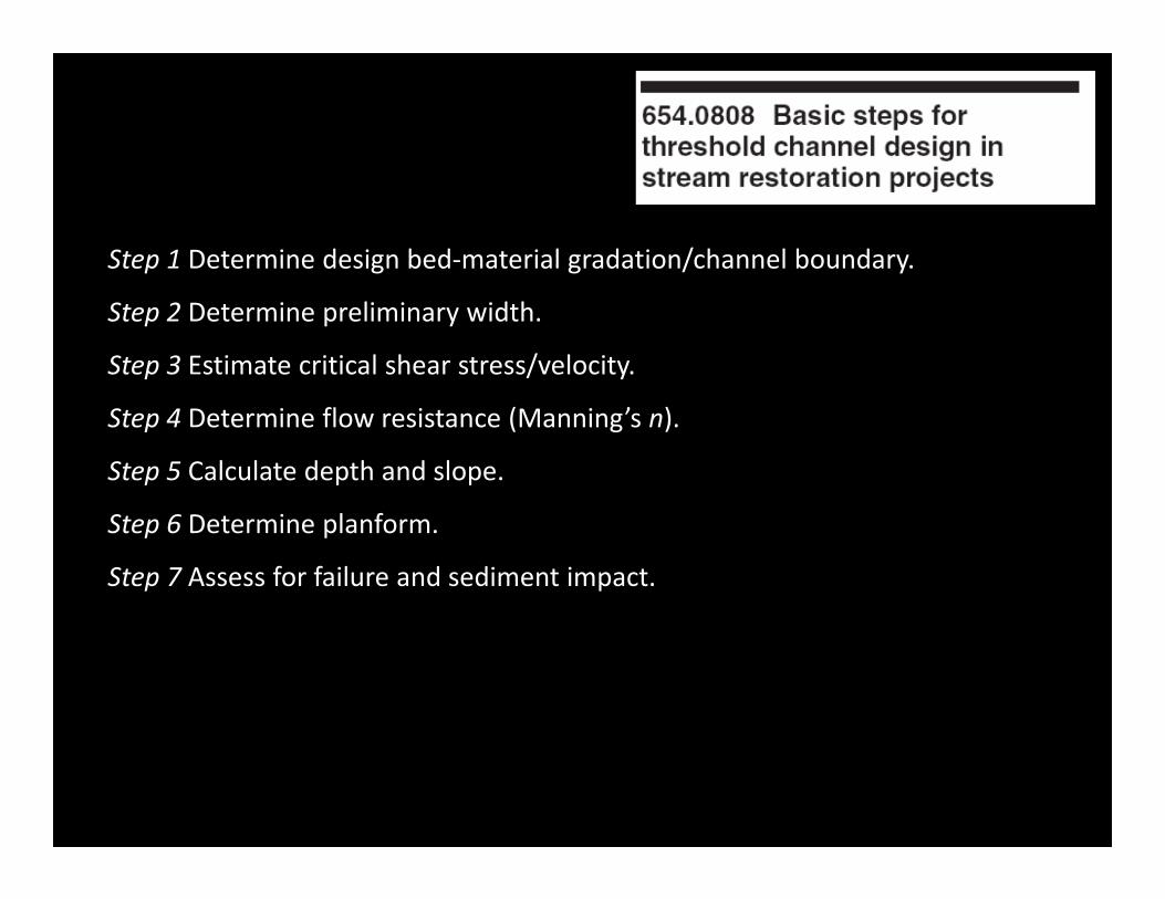
Step 1 Determine design bed‐material gradation/channel boundary.

Step 2 Determine preliminary width.

Step 3 Estimate critical shear stress/velocity.

Step 4 Determine flow resistance (Manning’s n).

Step 5 Calculate depth and slope.

Step 6 Determine planform.

Step 7 Assess for failure and sediment impact.

*0 c 50 84

*50

1/6lim

2/523/5

1

2

Given , , , and ,find , , , and from

( -1)

0.1129

1.16 2.03log84

2 1

2 1

c

c c

o nn

o n

o

o

c

Q B D Dn R U S

s gD

RnR

D

B h mnQhB mhS

h B mhARP B h m

QUA

Sgh

5/3

2/32

2 2

Finding Normal Depth - Trapezoidal Channel

( )Manning's eqn:

2 1

where

2 , , 2 1Finding , , or is easy; to find requires iteration

Try Mann

o

o

o o o o

h B mhSQn

B h m

B B mh A B h mh h B mh P B h mn Q S h

2/523/5

1

2 1ing arranged as

where and 1 subscripts indicate successive approximations

o nn

o n

B h mnQh

B mhSn n

h

Bomh

m

1

mh

*Given discharge , grain size ,

critical Shields Number ,Limerinos roughness &trapezoidal channel shape,find slope producing incipient motion.

c

Q D

S

18

0

0.002

0.004

0.006

0.008

0.01

0.012

0.014

0

0.2

0.4

0.6

0.8

1

1.2

1.4

0 5 10 15 20 25

SlopeDep

th (m

)

Bottom Width (m)

Depth Slope

*

Given discharge , grain size , Limerinos roughness & trapezoidal channel shape,find slope producing incipient motion.

Specify 12.5 m and 0.047,solution is 0.0064 with depth 0.54 m

c

Q DS

BS h

Sv

* 0.047c

19

0

0.002

0.004

0.006

0.008

0.01

0.012

0.014

0

0.2

0.4

0.6

0.8

1

1.2

1.4

0 5 10 15 20 25

SlopeDe

pth (m

)

Bottom Width (m)

DepthD = 32 mm, t* = 0.03SlopeD = 32 mm, t* = 0.03

*

*

Other values of , , and could be chosen

Changing 0.047 0.030 and 45 mm 32 mmc

c

n D

D

6( 1)

1 10/77 *( 1)

bb

cc

aQS s Dn

Sv

Calculated slope 3x bigger! = RISK

20

StrategyWhat is probability of failure? What probability are you willing to accept?

( ) ( ) ( )Choose width, slope combination to match acceptable risk.For example, for a 25yr and a cha

D D c

D

P failure P Q P Q Q

Q

nnel design with 10% failure probability,( ) ( ) ( ) (0.04)(0.1) 0.004

giving a 0.4% chance of failure in any year.D D cP failure P Q P Q Q

Qc

(II) The Armoring Problem

22

1. Stream‐bed armoringsurface composition &

the problem of predicting transport rates

Streambed Armoring

0

5

10

15

20

25

30

35

40

45

50

0-1 1-2 2-3 3-4 4-5 5-6 6-7 7-8 8-9 9-10

10-11

11-12

12-13

13-14

14-15

15-16

Armor Ratio

Freq

uenc

y

Mean: 2.80Std. Deviation: 2.06

Median: 2.16

Stream‐bed armoring is pervasive in gravel‐bed steams

Bed surface • grains available for transportcomposition • hydraulic roughnessdetermines: • bed permeability

• living conditions for bugs & fish

Armor Ratio =

D50 (surface) D50 (subsurface)

The armor problem

• We can measure the bed surface size at low flow, but not at flows moving sediment

• We don’t know what the bed surface looks like at the flows that create it

• Does the armor layer stay or goduring floods?

Q

Q

Qs

Q

Q Qs

Qs

Bed S f

Transport

Bed

Transport

D50

0

0.5

1

D50

Transport D50Surface D50

Flow, Transport Rate Flow, Transport RateFlow, Transport Rate

Sediment FeedSediment

Recirculation Both Cases

Mobility – driven armoring

Zero divergenceKinematic sorting

Flume studies do notresolve the issue

%

Grain Size

Q

To address the armor problem, we first tackle the transport problem

• Transport rates depend on transport of grains available for transport on bed surface

• But nearly all transport data provide composition of the bed subsurface, not surface!

• This means that the resulting transport models must somehow implicitly account for surface sorting (armoring)

Transport Modeling Basics ‐ 1

)sed , , , ,( miibi DDffnq

sed),/,(

),(

2

1

mimri

rii

bi

DDDfn

fnf

q

Given fully rough flow with boundary stress ,sediment of mean size Dm, with individual fractions of size Di and proportion fi. Transport rate qbi depends on

where sed = other sediment properties. We search a transport model of form

But, what size distribution should we use for fi ?

ans: surface

where ri is a reference value of near the onset of sediment motion

There were essentially no surface‐based transport observations, so we made some

• 5 sediments, add sand to gravel

• Sand: 0.5 – 2.0 mm• Gravel: 2.0 – 64 mm• Sand Content:

6, 14, 21, 27, & 34%• 9 or 10 runs with each

sediment, wide range of transport rates

• Depth & width held constant, primary variables are sand content & flow strength

0

5

10

15

0

5

10

15

y

0

5

10

15

y

0

5

10

15

J06

J14

J21

J27

BOMC

0

5

10

15

64.0

32.0

16.08.0

4.0

2.0

0.7

0.4

0.2

BOMC

0.25 0.5 421 8 16 32

Grain Size (mm)

SandGravel%

%

%

%

%

Transport Modeling Basics ‐ 2

),(1 rii

bi fnFq

To develop a general transport model, we nondimensionalize

in the form of a similarity collapse

rii fnW

3*

where 2/3

*

/)1(i

bii

FgqsW

gr. spec. sed density; water

gravity; ;proportion surface

s

gFi

The Point:The transport function does not contain grain size!

Building a surface‐based transport model

0.0001

0.001

0.01

0.1

1

10

1 10 100

0.711.191.682.383.364.766.739.5113.519.026.938.153.8treftr fn

(Pa)

*iW

0.0001

0.001

0.01

0.1

1

10

0.1 1 10 ri

*iW

*rW

Sediment = J14 Sediment = J14

*rW

It remains to explain ri …

1

10

100

0.1 1 10 100Grain Size Di (mm)

ri

Sediment = J14

Surface‐Based Transport Model

All sizes,All runs,

All sediments

0.00001

0.0001

0.001

0.01

0.1

1

10

0.1 1 10 100

*iW

ri /

Values of ri for all sizes and all sediments

0.1

1

10

100

0.1 1 10 100

J06 J14J21 J27BOMC ShieldsSurface Dm

Grain Size (mm) Di

r i

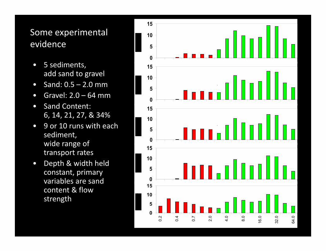
Values of ri collapse nicely when divided by values at the mean size Dsm

0.1

1

10

0.01 0.1 1 10 100

J06J14J21J27BOMCA 'hiding' function

r i rsm

D i D sm

Relative size effect weaker for larger sizes(absolute size effect makes ri increase with Di)

Wilcock, P.R. & Crowe, J.C., J. Hydr. Eng., 2003

It remains to explain rm …

Sand Interaction Function

The sand interaction function completes the surface‐based transport model

Surface‐based transport model can be used in both forward & inverse forms

• Forward: predict transport rate & grain sizeas function of and bed surface grain size

• Inverse: predict and bed surface grain sizeas function of transport rate & grain size

The inversemodel provides a useful tool for considering armor persistence – because we do have good transport data from the field

Don’t try this with a subsurface –based model!

To the field!

Transport grain size increases with flow!

iSBTM not only predicts a persistent armor layer, it also predicts the surface grain size observed in the field!

0

1020

30

4050

60

70

8090

100

0.1 1 10 100 1000

0.00025 0.000250.0013 0.00130.0042 0.00420.0072 0.00720.033 0.0330.11 0.11Surface

Grain Size (mm)

Perc

ent F

iner

Oak Ck, ORGrain size of transport (measured) and bed surface (calculated)

Transport Rate (kg/ms)(a)

1

10

100

0.0001 0.001 0.01 0.1 1

Surface D50Transport D50

(b)

Transport Rate (kg/ms)

Med

ian

Gra

in S

ize

(mm

)

Solid symbols: predicted surface grain size

Again, transport grain size increases with flow!

Again, iSBTM predicts a persistent armor layer. This time it overpredicts the surface grain size observed in the field!

Reason: dunes!

0102030405060708090

100

0.1 1 10 100

0.002 0.0020.011 0.0110.056 0.0560.185 0.1850.706 0.706SURF

Grain Size (mm)Pe

rcen

t Fin

er

Goodwin Ck MSGrain size of transport

(measured) and bed surface (calculated)

(a) Transport Rate (kg/ms)

0.1

1

10

100

0.001 0.01 0.1 1

Surface D50Transport D50

(b)

Transport Rate (kg/ms)

Med

ian

Gra

in S

ize

(mm

)

Solid symbols: predicted surface grain size

At “reach” and “storm” scales of space and time

• Armor layer grain size appears to be persistent – a real advantage for predicting roughness & transport during floods: a low flow measurement of bed composition may suffice (unless dunes develop)

Increasing transport grain size balances change in grain mobility to produce a constant bed surfaceA SBTM needed to model transients

(III) Sediment Transport in Alluvial Channel Design – reconnaissance,

planning, and design phases

41

Connecting sediment supply to the design problem1. Reconnaissance phase: What is the trajectory of the stream? How has it

responded to changes in water and sediment supply over the years? {Henderson relation mixed‐size seds}

2. Develop flood series, specify flood frequency Qbf.{Select Qbf for flood frequency specified to maintain riparian ecosystem & prevent vegetation encroachment}

3. Estimate sediment supply

4. Planning phase: What slope S is needed to carry the sediment supply with the available flow? {How does S vary with Qs and width b?}

5. Develop flow duration curve

6. Design phase: Evaluate trial designs. Will the sediment supply be routed through the reach over the flow duration curve?{Build 1‐d hydraulic model for trial design. Calculate cumulative transport over flow duration curve at each section; evaluate sediment continuity.}

Lane/Borland “Stable Channel” Balance (USBR 1955‐1960)

Sediment Supply Transport Capacity

This defines the controls for an alluvial channel

Reconnaissance

3

33/ 2

3/ 2

3 23

3/ 2

2 2

3/ 2

3/ 4

3/ 422 2 1

1 1 1 2

Einstein-Brown depth-slope continuity Chezy

* ( *)

( )

or

or for two cases

b

b

b

b

b

b

q RS q UR U RS

q q R SDRS qq R

SDq SqDq D

Sq

qS D qS q D q

The Lane Balance, quantified almost 40 yrs agoby Henderson (1966, Open Channel Flow)

What if qb increases and D decreases? Lane’s balance is indeterminate.

Reconnaissance

Pay attention to this slide

Surface‐based transport model can be used in both forward & inverse forms

• Forward: predict transport rate & grain sizeas function of and bed surface grain size

• Inverse: predict and bed surface grain sizeas function of transport rate & grain size

Don’t try this with a subsurface –based model!

We can use an inverse transport model to forecast, or design, a steady state channel that will transport a specified sediment supply rate and grain size with the available flow (!)

1. State Diagram I –transport v. discharge, lines of constant slope

2. State Diagram II –transport v. slope, lines of constant discharge

3. Channel Stability Diagram

Presenting ….

iSURF

• Inverse Model: predict and bed surface grain size as fn(transport rate & grain size)

• Specify discharge and basic channel geometry and solve for slope (& depth)

• Conservation RelationsWater Mass Momentum

• Constitutive RelationsRoughness relationSediment transport Flow resistance 2 / 3SU h

n

q UhghS

"Given": , , , , ,"Find": , , , , ,

t i s

i

q q p gU h S F n

gives , iiSBTM F

Stream State Diagrams

( )in f F

*3/ 2( 1)

tt

s

qqs gD

*3/ 2( 1)

ww

s

qqs gD

: Surface grain size: Transport grain size

i

i

Fp

We are working per unit width …The iSBTM routine calculates bed shear stress and bed surface grain size for a specified transport rate and transport grain size. Each transport rate and grain size and, therefore, shear stress and bed surface grain size, can be produced by different combinations of unit discharge q and slope S. The state diagrams present families of curves giving either transport rate and water discharge for specified values of S, or transport rate and S for specified values of water discharge.

Reconnaissance

0.01

0.1

1

10

100

0.01 0.1 1 10 100

Sedi

men

t Tra

nspo

rt R

ate

per u

nit w

idth

qT

(kg/

m/s

)

Water Discharge per unit width qW (m2/s)

S=0.001

S=0.002

S=0.005

S=0.01

S=0.02

S=0.05

G1=25.07,G2=25.07

G1=16.85,G2=16.85

G1=2.79,G2=2.79

Lines of constant slope

0.001

0.01

0.1

0.01 0.1 1 10 100

qw=0.10 m^2/s

qw=0.32

qw=1.0

qw=3.2

qw=10.0

G1=25.07,G2=25.07

G1=16.85,G2=16.85

G1=2.79,G2=2.79

Lines of constant unit water discharge

Slop

e

Sediment transport Rate per unit width qT (kg/m/s)

High slope

Low slope

Less armored

More armored

Less armoredMore armored

High flow

Low flow

Reconnaissance

GivenWater discharge and sediment supply

Findchannel

slope, depth & width(& velocity & shear)

We have enough general relations to solve for all but one of these unknown variables

If we specify channel width, we can solve for the rest of the variables

What slope is needed to transport the supplied sediment with the available water?

How big the channel?Planning

Hydraulic Design of Stream Restoration Projects September 2001RR Copeland, DN McComas, CR Thorne, PJ Soar, MM Jonas, JB Fripp

For a specified supply of water and sediment, what is the slope needed to transport the supplied sediment

with the available flow?Planning

Sometimes, sediment supply does not matter

Sometimes, it does

1

10

100

1000

1 10 100 1000 10000

AlbertaBritain IIdahoColorado RBritain IIMarylandTuscany

Bankfull Discharge (cms)

Ban

kful

l with

(m)

So, there must be a boundary between cases where sediment supply matters or not

Threshold AlluvialBed & banks immobile Active transport

Easier to model & designBed & banks must only be

strong enough

Harder to designRequires a balance

between transport capacity & sediment supply

Extend Threshold definition to include small sediment supply rates requiring a

slope negligibly larger than the zero supply case

Focus on cases in which slope is sensitive to supply

Nothing new under the sun … see SCS in the ’30s

Why we can ‘neglect’ small sediment supply rates

1. Small sediment supply rates many storms (and many decades) req’d to produce significant aggradation and degradation.

2. Small sediment supply rates channel morphology and slope required to transport the supplied sediment can be negligibly larger than that of a threshold channel.

So, what is a SMALL sediment supply rate?That sounds dangerously like a real question, so first, lets deal with real sediments, which contain a mixture of sizes

But for mixed‐size sediment, there are complications … • Grain size of bed grain size of transport • Bed is sorted spatially and vertically• Transport is a function of the changing population of grains on

the bed surface

iSURF Channel Stability Diagramwhat slope is needed to transport a specified sediment supply of specified size distribution with a specified discharge?

Find velocity, boundary stress, depth, slope, and bed surface grain size fromcontinuity, momentum, flow resistance, and the Wilcock‐Crowe Surface‐Based Mixed‐Size Sediment Transport Model

hm

1

b

Channel Stability Diagram

As a bonus, you find out how armored the bed becomes !

0

0.001

0.002

0.003

0.004

0.005

0.006

0.007

5 10 15 20 2500.20.40.60.811.21.41.61.8

Slope Case 1 Slope Case 2Depth Case 1 Depth Case 2

Channel Width (m)

Slo

pe

Depth (m

)

Discharge 1 = 17.0 Discharge 2 = 17.0

Sed Supply 1 = 954 kg/hr


0

0.005

0.01

0.015

0.02

0.025

0.03

1 10 100 1,000 10,000 100,000 1,000,000

Case 1Case 2Your sediment supply

Sediment Supply Rate (kg/hr)

Slo

pe

Discharge 1 = 17.0 cms


b = 14.0 m

0

20

40

60

80

100

0.1 1 10 100 1000Grain Size (mm)

Case 1 TransportCase 2 TransportCase 1 Bed SurfaceCase 2 Bed Surface

% F

iner

b = 14.0 m

And get a measure of where you are relative to the threshold/alluvial channel boundary !

Planning

0

0.001

0.002

0.003

0.004

0.005

0.006

0.007

1 10 100 1,000 10,000 100,000 1,000,000

Q = 70.8 cms

Your sediment supply


Slo

peb = 19.0 m

If your sediment supply is safely below the boundary between “low” slope and “high” slope, channel slope is relatively insensitive to sediment supply – you are less likely to accumulate sediment given an error in estimating sediment supply

threshold

Is an accurate sediment supply estimate needed?

Threshold Design Approach Just make the channel strong enough to stand up to high flows

1. Reconnaissance phase: What is the trajectory of the stream? How has it responded to changes in water and sediment supply over the years?

2. Develop flood series, specify flood frequency Design Q.{Select Qbf for flood frequency specified to maintain riparian ecosystem & prevent vegetation encroachment}

3. Estimate sediment supply

4. Planning phase: What slope S will transportthe sediment supply with the available Qbf? Calculate (b, S) combination {S and valley slope determine sinuosity}

Check if alluvial v. threshold channel

5. Develop flow duration curve

6. Design phase: Evaluate trial designs. Will the sediment supply be routed through the reach over the flow duration curve?{Build 1‐d hydraulic model for trial design. Calculate cumulative transport over flow duration curve at each section; evaluate sediment continuity.}

7. Bottlenecks or blowouts? Adjust for sediment continuity

3/ 422 2 1

1 1 1 2bb

qS D qS q D q

0

0.002

0.004

0.006

0.008

0.01

0.012

0 5 10 15 200

0.5

1

1.5

2

2.5

3

3.5

Slope Case 1 Slope Case 2Depth Case 1 Depth Case 2

Channel Width (m)

Slop

e Depth (m

)

Discharge 1 = 15.0

Discharge 2 = 25.0



0

0.005

0.01

0.015

0.02

0.025

1 10 100 1,000 10,000 100,000 1,000,000

Case 1Case 2Your sediment supply


Slo

pe



b = 11.0 m

Design steps incorporating sediment supply

iSURF State Diagrams

Some Design DetailStep-backwater model gives S(Q), U(Q) at each section

Grain stress:

Calculate transport over the flow dur. curve at each section

Adjust x/s transport for lateral variation in

Query potential bottlenecks, blowoutstransport < capacity?flow model reliable?erosion/deposition desirable?

Adjust channel dimensions & shapeto match supply, within tolerance level & design objectives.

1/ 4 3/ 265' 17 SD U

Use transport modeling to:i. Evaluate design, esp. Qs from section to sectionii. Determine if more accurate transport modeling is needed

0.0010.010.1

110

1001000

10000100000

1000000

24 26 28 30 32 34 36 38 40 42 44

Cum Qb * lateral correction (skn)

Section

Tran

spor

t (M

tons

)

Q = 1600 cfs

3/ 2' D

onn

Design

(IV) Alluvial Channel Design Example

60

(70.8 m3/s)

(6.7 m)

1. Supply reachEstimate sediment transport rate

2. Design reachGiven discharge and sediment supply rate and grain size, calculate slope needed to transport supplied sediment at a specified channel width

Design

NEH-654 Chapter 9 Example 2, p. 39Given geometry of a trapezoid channel w/specified bed material and side roughness,find boundary and grain stresses

Q 70.79 cmsS 0.0025

D50 3.7 mmD84 22 mmm 1.6nD 0.022ns 0.07

Bo nc h B A R U o ' u*'m composite n m m m^2 m m/s Pa Pa m/s

6.71 0.0369 2.97 16.2 34.0 1.90 2.08 46.6 21.1 0.145total Grain Grain

Bo nc h B A R U boundary stress stressft ft ft ft^2 ft ft/s stress as a shear

22.0 0.0369 9.74 53.2 366.3 6.23 6.83 velocity

Enter information only in green cells!!No cutting and pasting!

No inserting or deleting rows!

F

M

w

F

T

B

w

1. Find stress in upstream “supply” channel

SBTM - calculate transport rate and transport grain size fromspecified shear velocity and bed surface grain size

RULES, CONVENTIONS, AND UNITS1. Cells for input data are highlighted in GREEN, cells for output data are ORANGE2. Grain-diameters must be in millimeters (mm)3. Cumulative percentiles, not fractions, are used4. Cumulative grain-size distribution percentiles must span from 0 to 100 %5. Shear velocity must be in meters-per-second (m/s)6. The 0 and 100 % must be EXACTLY 0 and 100INSTRUCTIONS1. In table below, enter grain size and cumulative % in order of decreasing grain size2. Enter your bed shear velocity3. Check input for errors, press Enter , and then click once on the Run SBTM button

Parameter Value Description Unitsu* 1.45E-01 Bed shear velocity m/sqT 8.17E-04 Total transport rate m2/s

D (mm) Surface CDF GSD (% Finer) Transport CDF GSD (% Finer)64.00 100.00 100.0032.00 93.00 98.8616.00 77.00 93.038.00 65.00 84.944.00 53.00 72.392.00 45.00 62.511.00 35.00 49.350.50 20.00 28.820.25 10.00 14.650.13 0.00 0.00

2. Find transport rate in upstream “supply” channel

Parameter Value Description UnitsQ 1 70.8 Case 1 water discharge m3/s

Q T1 0.005478475 Case 1 sediment supply rate m3/s

Q 2 70.8 Case 2 water discharge m3/s


b min 3.00 Minimum bottom width mb max 35.00 Maximum bottom width m

D (mm) Case 1 Transport Grain Size (% Finer)

Case 2 Transport Grain Size (% Finer)

64.00 100.00 100.0032.00 98.86 98.8616.00 93.03 93.038.00 84.94 84.944.00 72.39 72.392.00 62.51 62.511.00 49.35 49.350.50 28.82 28.820.25 14.65 14.650.13 0.00 0.00

3. Enter transport rate and grain size from upstream “supply” channel as input to the channel stability code

0.001

0.0015

0.002

0.0025

0.003

0.0035

0.004

0 5 10 15 20 25 30 35

Slope Case 1 Slope Case 2 NRCS

Channel Width (m)

Slo

pe





Sv

iSURF (Wilcock&Crowe) solutionincluding case with 3x sediment supply

Potential Degradation

Potential Aggradation

0

0.001

0.002

0.003

0.004

0.005

0.006

0.007

1 10 100 1,000 10,000 100,000 1,000,000

Q = 70.8 cms



Slo

peb = 19.0 m

For this design problem, slope is very sensitive to sediment supply rate

(because it is large)

iSURF design module provides this plot of slope vs. sediment supply rate

A simple example of all three channel types

h

Bomh

2

1

mh 3 3

50

100 m /s {160 m /s}20 t/hr {60 t/hr}

Supply 13 mm (0.5 mm - 128 mm)s

QQ

D

3

50

84

*

100 m /s64 mm128 mm 10%

0.04 10%

0.03 10%c

QDDn

Pay attention to the next four slides!

0

0.6

1.2

1.8

2.4

3

3.6

0

0.001

0.002

0.003

0.004

0.005

0.006

0.007

10 20 30 40 50

Bottom Width (m)

Slop

e

Channel D

epth (m)

Slope

Depth

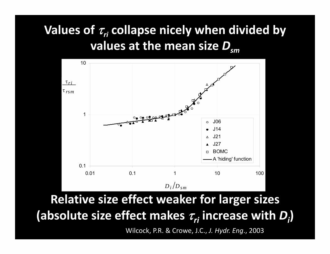
h

Bomh

2

1

mh 3

50

84

*

100 m /s64 mm128 mm 10%

0.04 10%

0.03 10%c

QDDn

Failure in a threshold channel = grain entrainment

h

Bomh

2

1

mh 3 3

50

100 m /s {160 m /s}20 t/hr {60 t/hr}


QQ

D

Mobile channel design = match transport capacity to sediment supply

0

0.001

0.002

0.003

0.004

0.005

0.006

10 20 30 40 50

Bottom Width (m)

Threshold Slope

Alluvial 100/20

Alluvial 160/60Sl

ope

h

Bomh

2

1

mh 3 3

50

100 m /s {160 m /s}20 t/hr {60 t/hr}


QQ

D

3

50

84

*

100 m /s64 mm128 mm 10%

0.04 10%

0.03 10%c

QDDn

Over‐capacity Threshold: combine threshold and alluvial

0

0.001

0.002

0.003

0.004

0.005

10 20 30 40 50

Bottom Width (m)

Threshold Channel

Alluvial Balance

Slop

e

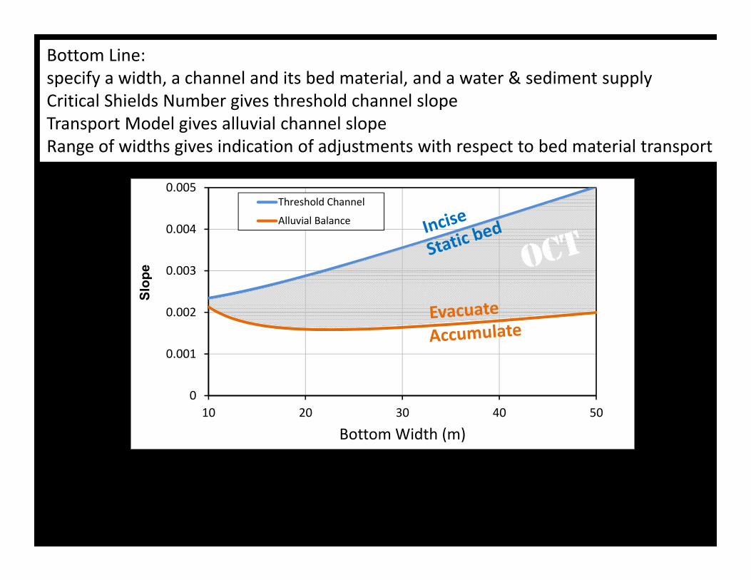
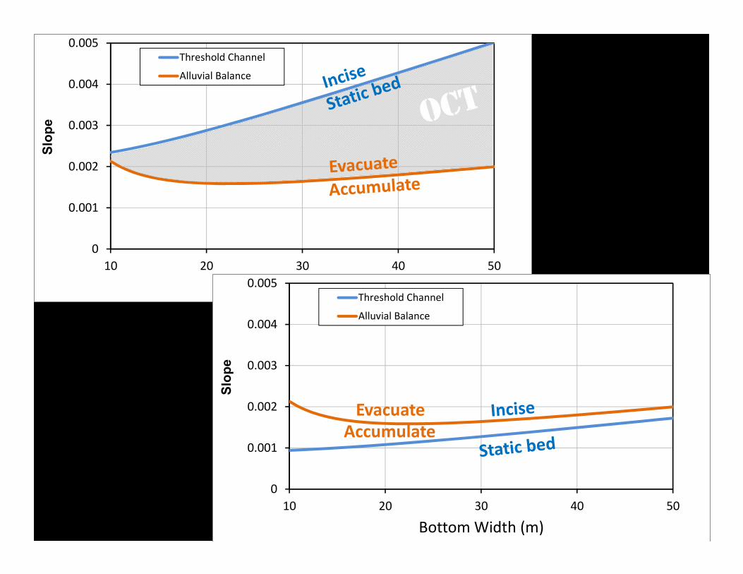
Bottom Line:specify a width, a channel and its bed material, and a water & sediment supplyCritical Shields Number gives threshold channel slopeTransport Model gives alluvial channel slopeRange of widths gives indication of adjustments with respect to bed material transport

0

0.001

0.002

0.003

0.004

0.005

10 20 30 40 50

Bottom Width (m)

Threshold Channel

Alluvial Balance

Slop

e

0

0.001

0.002

0.003

0.004

0.005

10 20 30 40 50

Bottom Width (m)

Threshold Channel

Alluvial Balance

Slop

e

EvacuateAccumulate

0

0.001

0.002

0.003

0.004

0.005

10 20 30 40 50

Bottom Width (m)

Threshold Channel

Alluvial Balance

Slop

eDischarge

Rate of Sediment Supply

Grain Size of Sediment Supply

But the watershed, and the water and sediment supply may also be changingaka ‘moving the goalposts’

Arrows indicate response to an INCREASE in each driving variable

(V) Channel Design Strategy

74

Strategy(i) Determine if the sediment supply is a big number or a little number

(a) if big, invest in more accurate estimate of sediment supplybe prepared for a dynamic channel reserve riparian corridor and let the stream go

or plan to trap and remove sediment(b) if little, design a threshold channel

(ii) Estimate uncertainty and account for the consequencesesp. potential for aggradation, degradation

0

0.001

0.002

0.003

0.004

0.005

0.006

0.007

1 10 100 1,000 10,000 100,000 1,000,000

Q = 70.8 cms



Slo

pe

b = 19.0 m

OR, Make your channel(i) steep enough: transport capacity

exceeds supply and(ii) strong enough: bed material immobile

… an overcapacity threshold channel

Design Basis: Flow Competence

Competence & Capacity

Transport Capacity

Channel Type Threshold Channel

Overcapacity Threshold

Alluvial Channel

Topography & Bed Material

Static Static Dynamic

Pipe‐like channels: an increasingly common & safe design option,may provide acceptable aesthetics.

Does not provide anything like native structure & function

Assess magnitude of sediment supply

“small” “large”

Threshold channel design

Use risk assessment and P(failure) to guide design

Alluvial channel design

Allow for dynamic stream

Invest in improved sediment estimate

Overcapacity channel design

Objectivesediment & nutrients

property & infrastructurebiological recovery

aesthetics, recreationpenance

Whatneeds

fixing?

Stormwater control

Nothing

Channel change

Introduced species Disturbance Internal orexternal?

InternalExternal

Fence out the cows!Remove the concrete!

Template approachcan work

Channel DesignSediment Objectives

Is Sediment Supply Large or Small?

Estimate flood frequency

Design threshold channel

Estimate sediment supply & flow

durationDesign alluvial

channel

Alluvial, Threshold, or Overcapacity Threshold Channel?

…

Sediment Transport in Channel DesignE

nvir

onm

enta

l D

rive

rs

Design Threshold AND

Alluvial Channel

We can go beyond equilibrium channel design by Specifying desired channel behavior and

incorporating sediment transport with uncertainty, Which allows calculation of risk of undesirable behaviorwhile accommodating “typical” channel dimensions

Channel DesignSpecified

equilibrium dimensions

Specified channel behavior

Account for uncertainty & riskAccommodate typical dimensions

iSURF does Provo 2016

PRRP OFFICE

0.01

0.1

1

10

100

1000

100 1000 10000

White BridgeRiver RDMidwayCasperville

Discharge (cfs)

Tran

spor

t Rat

e (to

ns/d

ay)

Does not include transport samples <1g for the 2-16mm size class

2-16 mm

1

10

100

1000

100 1000 10000

River RDMidwayCasperville

Discharge (cfs)

Tran

spor

t Rat

e (to

ns/d

ay)

Does not include transport samples <200g for the >16mm size classNo meaasured transport in this size range at White Bridge

> 16 mm

Transport Observations by BioWest Inc.

iSURF Channel Stability Diagram for 1200 cfs and 1800 cfs flowsCHANNEL STABILITY DIAGRAM FOR GRAVEL-BED RIVERS - INPUT WORKSHEET For the input entered below, here are max and min values of RULES, CONVENTIONS, AND UNITS water discharge per unit width1. Cells for input data are highlighted in GREEN Maximum q Minimum q2. Grain-diameters must be in millimeters (mm) 4.25 m 2̂/s 0.68 m 2̂/s Case 13. Cumulative percentiles, not fractions, are used 6.38 m 2̂/s 1.02 m 2̂/s Case 24. Cumulative grain-size distribution percentiles must span from 0 to 100 %5. The 0 and 100 % must be EXACTLY 0 and 100 For the input entered below, here are max and min values of INSTRUCTIONS sediment transport rate per unit width1. In first table below, enter water discharge and sediment supply rate in units of m3/s Maximum qs Minimum qs

and the minimum and maximum channel widths to be evaluated 0.00 kg/m/s 0.00 kg/m/s Case 12. In second table below, enter grain size and cumulative % in order of decreasing grain size 0.48 kg/m/s 0.08 kg/m/s Case 23. In cells to right, enter side slope angle z and side slope roughness ns4. Check input for errors and then click once on the Run STAB button this cell intentionally left blank5. Results appear on Worksheet "STAB OUTPUT"Parameter Value Description Units Parameter Value Description Units

Q 1 34 Case 1 water discharge m3/s z 1 side slope z:1 H:V 0Q T1 0.00000397 Case 1 sediment supply rate m3/s ns 0.08 side slope roughness #&%@$Q 2 51 Case 2 water discharge m3/s


b min 8.00 Minimum bottom width mb max 50.00 Maximum bottom width m

D (mm) Case 1 Transport Grain Size (% Finer)

Case 2 Transport Grain Size (% Finer)

128.00 100.00 100.0090.00 99.50 98.7064.00 97.60 90.0045.00 92.00 74.30 Statistic FIRST Transport GSD SECOND Transport GSD Units32.00 73.10 53.50 Dmin 1.00 1.00 mm22.00 50.40 32.60 Dmax 128.00 128.00 mm16.00 13.30 10.80 D50 21.92 30.05 mm8.00 9.70 7.10 Dg 20.52 26.85 mm4.00 7.50 5.30 g 1.18 1.24 /-units

2.00 4.30 4.20 Fs 4.30 4.20 %1.00 0.00 0.00

0

20

40

60

80

100

0.1 1 10 100Grain Size (mm)

GSD1

GSD2

% F

iner

Input transport size distributions

hz

b

Reset: inserts some harmless data and cleans up output cells

Run STAB

Reset

Channel Stability chart developed using inverse calculation of the Wilcock & Crowe (2003) transport relation. z 1 side slope z:1 H:V ns 0.08 side slope 1. CHANNEL STABILITY DIAGRAM 2. THRESHOLD CHECK - SLOPE AS FN(SEDIMENT SUPPLY RATE) AT MEAN WI

At b=29.0m U=1.6m/s qt=0.000kg/m/s3. GRAIN-SIZE DISTRIBUTIONS At b=29.0m U=2.3m/s qt=0.133kg/m/s

0

0.5

1

1.5

2

2.5

00.0010.0020.0030.0040.0050.0060.0070.0080.0090.01

0 10 20 30 40 50 60

Slope Case 1 Slope Case 2

Depth Case 1 Depth Case 2

Channel Width (m)

Slo

pe

Depth (m

)





0

0.005

0.01

0.015

0.02

0.025

0.03

1 10 100 1,000 10,000 100,000 1

Case 1

Case 2



Slo

pe Discharge 1 = 34.0 cms


b = 29.0 m

0

20

40

60

80

100

0.1 1 10 100Grain Size (mm)

Case 1 Transport

Case 2 Transport

Case 1 Bed Surface

Case 2 Bed Surface

% F

iner

b = 29.0 m

0.00.10.20.30.40.50.60.70.80.91.0

0

0.5

1

1.5

2

2.5

0 10 20 30 40 50 60

Armor Case 1 Armor Case 2

Froude # Case 1 Froude # Case 2

Channel Width (m)

Arm

or R

atio

Dsm

/Dtm Froude N

umber

iSURF Channel Stability Diagram for 1200 cfs and 1800 cfs flows

(VI) OvertimeThreshold & Alluvial Channel Design

from the guys who invented it

88

Some useful readings

89

Fortier and Scobey (1926)

Increased Bank Velocity in Bends

1.74 0.52log

: depth-averaged velocity at 20% slope length from toe: X/S average velocity

: bend hydraulic radius: channel top width

ssavg

ss

avg

V RV W

V

V

RW

3/ 21/ 6

0

c

1. Calculate total stress (use RAS if flow non-uniform)

2. Calculate grain stress ' using

' and 0.013

for in mm3. Choose critical Shields Number4. Compare ' and

DD

n n Dn

D

Step 1 Determine design bed‐material gradation/channel boundary.

Step 2 Determine preliminary width.

Step 3 Estimate critical shear stress/velocity.

Step 4 Determine flow resistance (Manning’s n).

Step 5 Calculate depth and slope.

Step 6 Determine planform.

Step 7 Assess for failure and sediment impact.

(70.8 m3/s)

(6.7 m)

1. Supply reachEstimate sediment transport rate

2. Design reachGiven discharge and sediment supply rate and grain size, calculate slope needed to transport supplied sediment at a specified channel width

Design

0.001

0.0015

0.002

0.0025

0.003

0.0035

0.004

0 5 10 15 20 25 30 35

NRCS

Channel Width (m)

Slo

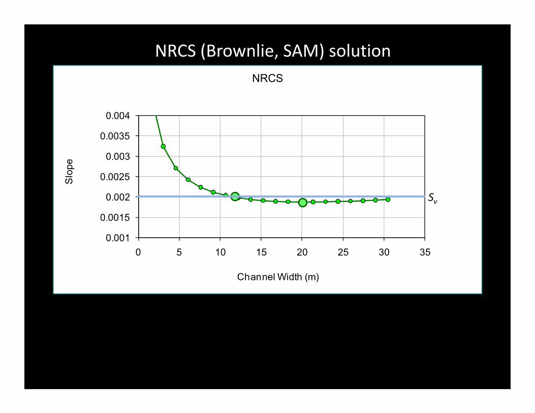
peNRCS (Brownlie, SAM) solution

Sv

Documents

Sediment Transport & Channel Design - QCNR | USU · Previous Experiments •Jackson & Beschta (1984) •Ikeda & Iseya (1988) Adding sand increases gravel mobility East Fk R., near