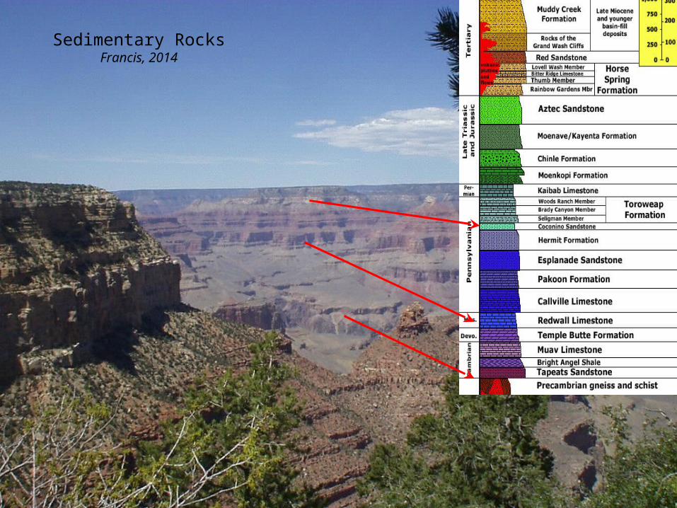
Sedimentary RocksFrancis, 2014

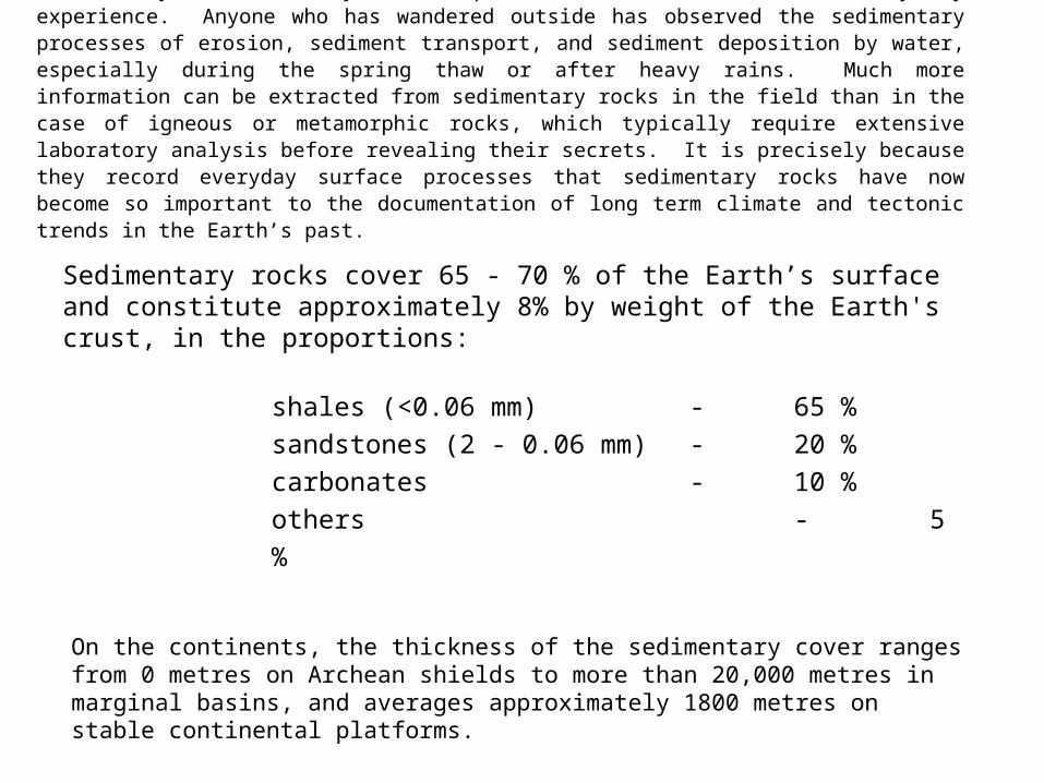
Sedimentary rocks cover 65 - 70 % of the Earth’s surface and constitute approximately 8% by weight of the Earth's crust, in the proportions:

shales (<0.06 mm) - 65 %

sandstones (2 - 0.06 mm) - 20 %

carbonates - 10 %

others - 5 %

On the continents, the thickness of the sedimentary cover ranges from 0 metres on Archean shields to more than 20,000 metres in marginal basins, and averages approximately 1800 metres on stable continental platforms.

Sedimentary rocks form by surface processes with which we have every day experience. Anyone who has wandered outside has observed the sedimentary processes of erosion, sediment transport, and sediment deposition by water, especially during the spring thaw or after heavy rains. Much more information can be extracted from sedimentary rocks in the field than in the case of igneous or metamorphic rocks, which typically require extensive laboratory analysis before revealing their secrets. It is precisely because they record everyday surface processes that sedimentary rocks have now become so important to the documentation of long term climate and tectonic trends in the Earth’s past.

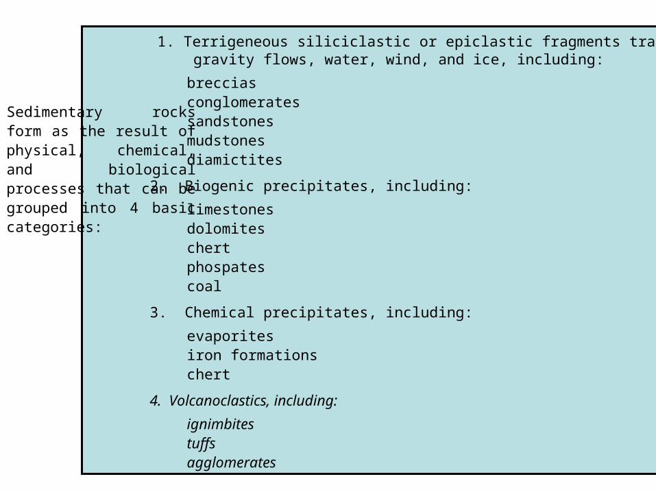
1. Terrigeneous siliciclastic or epiclastic fragments transported by gravity flows, water, wind, and ice, including:

brecciasconglomeratessandstonesmudstonesdiamictites

2. Biogenic precipitates, including:

limestonesdolomiteschertphospatescoal

3. Chemical precipitates, including:

evaporitesiron formationschert

4. Volcanoclastics, including:

ignimbitestuffsagglomerates

Sedimentary rocks form as the result of physical, chemical, and biological processes that can be grouped into 4 basic categories:

Relevance of Sedimentary Rocks and Stratigraphy

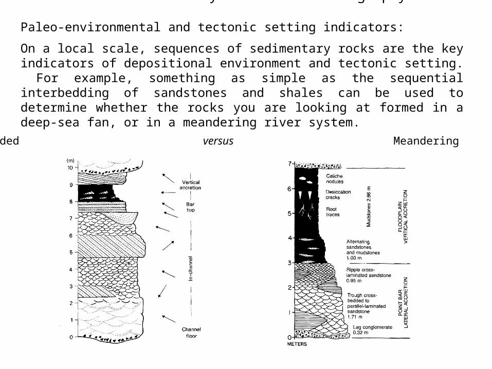
Paleo-environmental and tectonic setting indicators:

On a local scale, sequences of sedimentary rocks are the key indicators of depositional environment and tectonic setting. For example, something as simple as the sequential interbedding of sandstones and shales can be used to determine whether the rocks you are looking at formed in a deep-sea fan, or in a meandering river system.

Braided versus Meandering

Paleo-climatic indicators

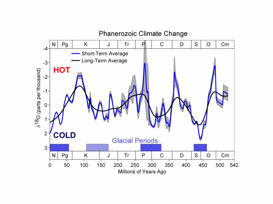
The current interest in climate change has heightened interest in the study of sedimentary sequences on a global scale as the systematic recorders of past climate change. For example, the detailed stratigraphic analysis of oxygen isotope compositions in limestone successions can be used to chart changes sea level, temperature, and compositional in time over the Earth’s history.

Phanerozoic : 500+ MysLate-Tertiary : 12 Mys

Sea Level Variations

sequence

boundary

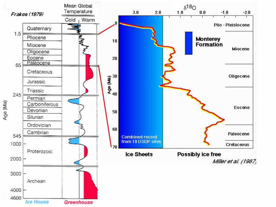
Analyses of the climate variation over the last few 100 thousand years reveals a strong inverse correlation between the concentration of CO2 in the atmosphere, δ18O, and the volume of polar ice.

Present CO2 concentration ~ 387 ppm

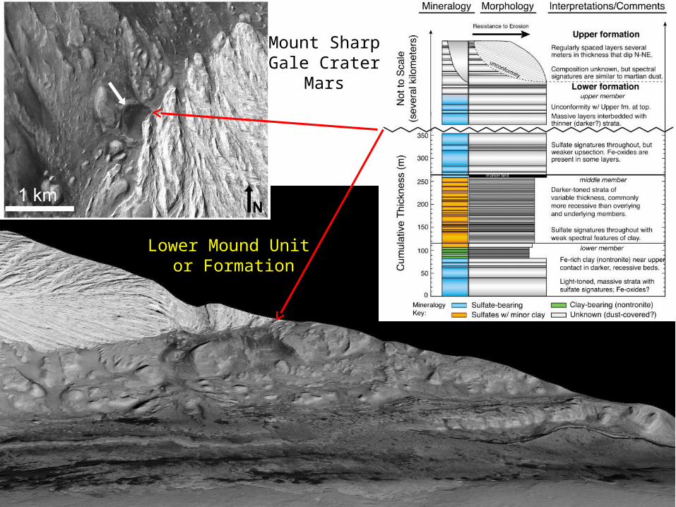
Lower Mound Unit or Formation

Mount SharpGale Crater

Mars

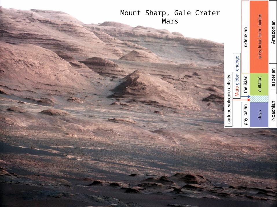
Mount Sharp, Gale CraterMars

Hosts to petroleum and economic minerals reserves:

Many important types of mineral deposits occur in sedimentary rocks; including:

- both exhalative and Mississippi valley-type Pb-Zn deposits.- red bed copper deposits.- paleo-placer deposits of Au and U. - Carlin-type gold deposits- Wyoming-type U deposits.- sources of salt, gypsum, phospates, nitrates, manganese, etc.

Sedimentary rocks form both the source rocks and the reservoirs for hydrocarbon reserves.

Indicators of metamorphic grade

We shall see in the final third of this course that mineral reactions in meta-sedimentary rocks are particularly useful for constraining pressures and temperature histories during metamorphism. This reflects their distinctive Al-rich composition compared to igneous rocks, a result of weathering that originally created the sediment.

Weathering

The majority of igneous minerals formed at temperatures in excess of 700oC and are unstable under atmospheric or submarine conditions. The action of weathering converts these high temperature minerals into three distinct types of material:

1) elements which are dissolved by water and carried off in solution:

- K, Na, Ca, Mg

2) materials which are ‘resistates’ and carried as clastic fragments:

- quartz, rutile, zircon, diamond, garnet, feldspar, magnetite

3) newly formed insoluble minerals and amorphous phases formed by the breakdown of unstable phases such as feldspars and mafic silicates: - clay minerals, hydroxides of Fe, Mn, and Al, silica

Physical Weathering:

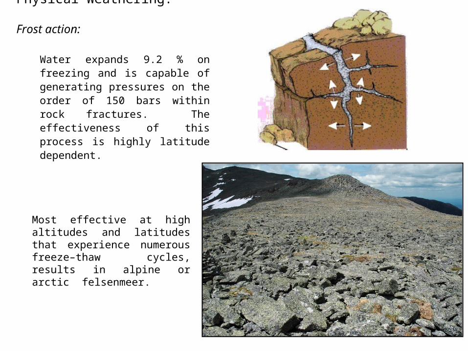
Frost action:

Water expands 9.2 % on freezing and is capable of generating pressures on the order of 150 bars within rock fractures. The effectiveness of this process is highly latitude dependent.

Most effective at high altitudes and latitudes that experience numerous freeze–thaw cycles, results in alpine or arctic felsenmeer.

Physical Weathering:

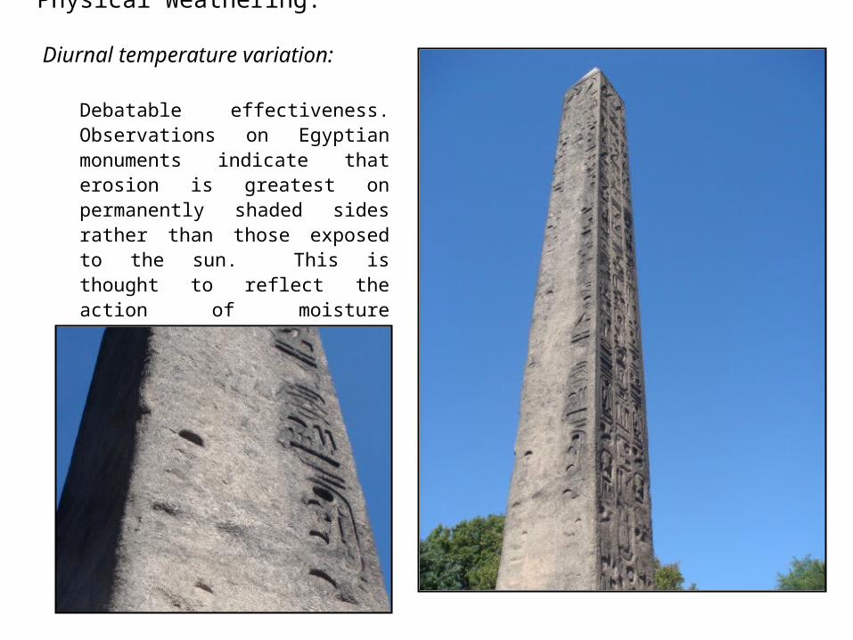
Diurnal temperature variation:

Debatable effectiveness. Observations on Egyptian monuments indicate that erosion is greatest on permanently shaded sides rather than those exposed to the sun. This is thought to reflect the action of moisture condensation on cool surface.

Physical Weathering:

Sheeting:

Many massive rock lithologies such, as granite, develop a sheet-like jointing parallel to the surface due to expansion following unloading by erosion. Expansion due to decreasing pressure during unroofing also tends to disaggregate coarse grained rocks such as granitoids, forming sand size clastic grains.

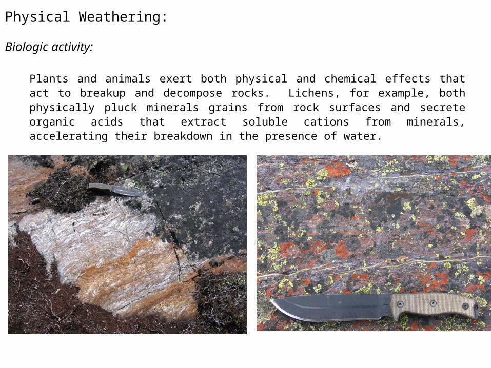
Physical Weathering:

Biologic activity:

Plants and animals exert both physical and chemical effects that act to breakup and decompose rocks. Lichens, for example, both physically pluck minerals grains from rock surfaces and secrete organic acids that extract soluble cations from minerals, accelerating their breakdown in the presence of water.

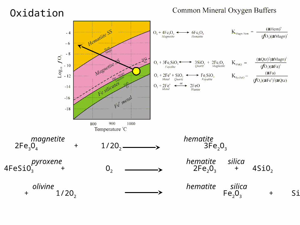
2Fe3O4 + 1/2O2 3Fe2O3

4FeSiO3 + O2 2Fe2O3 + 4SiO2

Fe2SiO4 + 1/2O2 Fe2O3 + SiO2

hematite

hematite

hematite

pyroxene silica

silica

magnetite

olivine

Oxidation

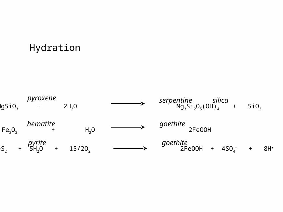
Hydration

3MgSiO3 + 2H2O Mg3Si2O5(OH)4 + SiO2

Fe2O3 + H2O 2FeOOH

2FeS2 + 5H2O + 15/2O2 2FeOOH + 4SO4= + 8H+

hematite goethite

goethite

pyroxene

pyrite

serpentine silica

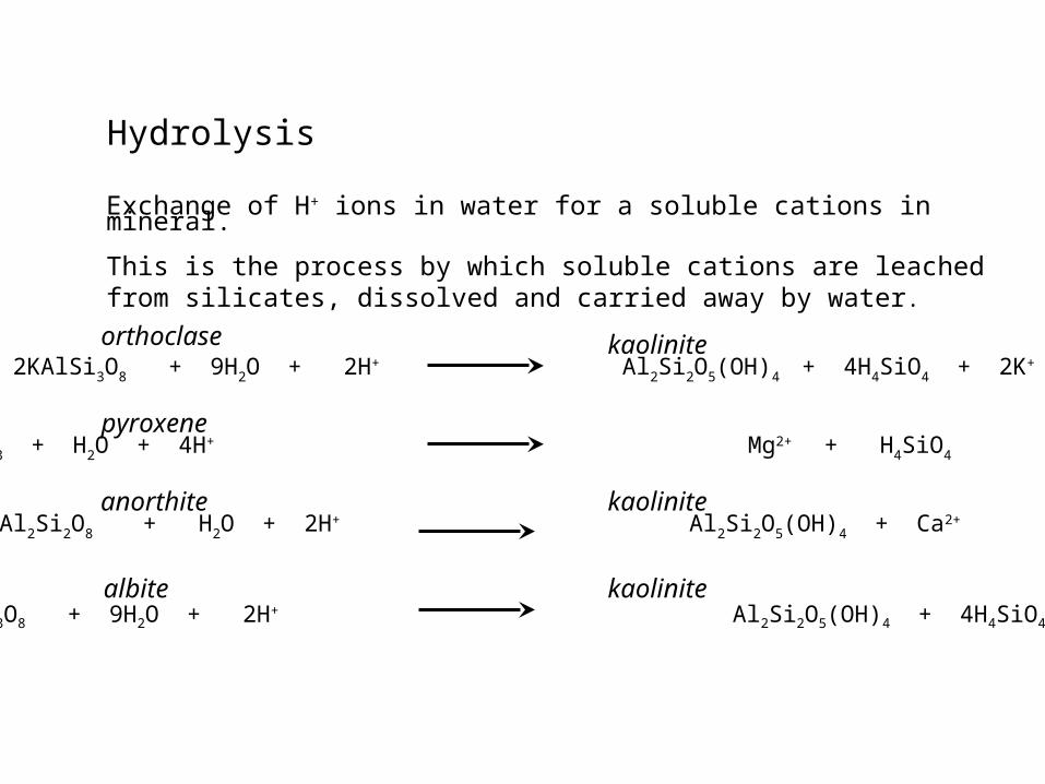
Hydrolysis

2NaAlSi3O8 + 9H2O + 2H+ Al2Si2O5(OH)4 + 4H4SiO4 + 2Na+

MgSiO3 + H2O + 4H+ Mg2+ + H4SiO4

CaAl2Si2O8 + H2O + 2H+ Al2Si2O5(OH)4 + Ca2+

2KAlSi3O8 + 9H2O + 2H+ Al2Si2O5(OH)4 + 4H4SiO4 + 2K+

pyroxene

orthoclase

anorthite

albite kaolinite

kaolinite

kaolinite

Exchange of H+ ions in water for a soluble cations in mineral.

This is the process by which soluble cations are leached from silicates, dissolved and carried away by water.

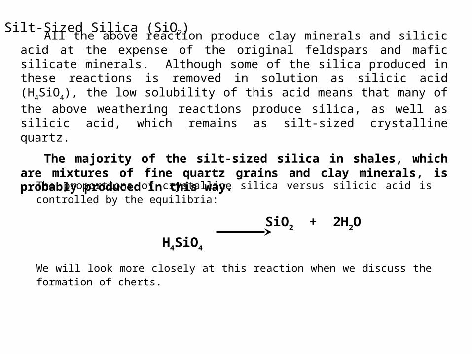
All the above reaction produce clay minerals and silicic acid at the expense of the original feldspars and mafic silicate minerals. Although some of the silica produced in these reactions is removed in solution as silicic acid (H4SiO4), the low solubility of this

acid means that many of the above weathering reactions produce silica, as well as silicic acid, which remains as silt-sized crystalline quartz.

The majority of the silt-sized silica in shales, which are mixtures of fine quartz grains and clay minerals, is probably produced in this way.

The proportions of crystalline silica versus silicic acid is controlled by the equilibria:

SiO2 + 2H2O H4SiO4

We will look more closely at this reaction when we discuss the formation of cherts.

Silt-Sized Silica (SiO2)

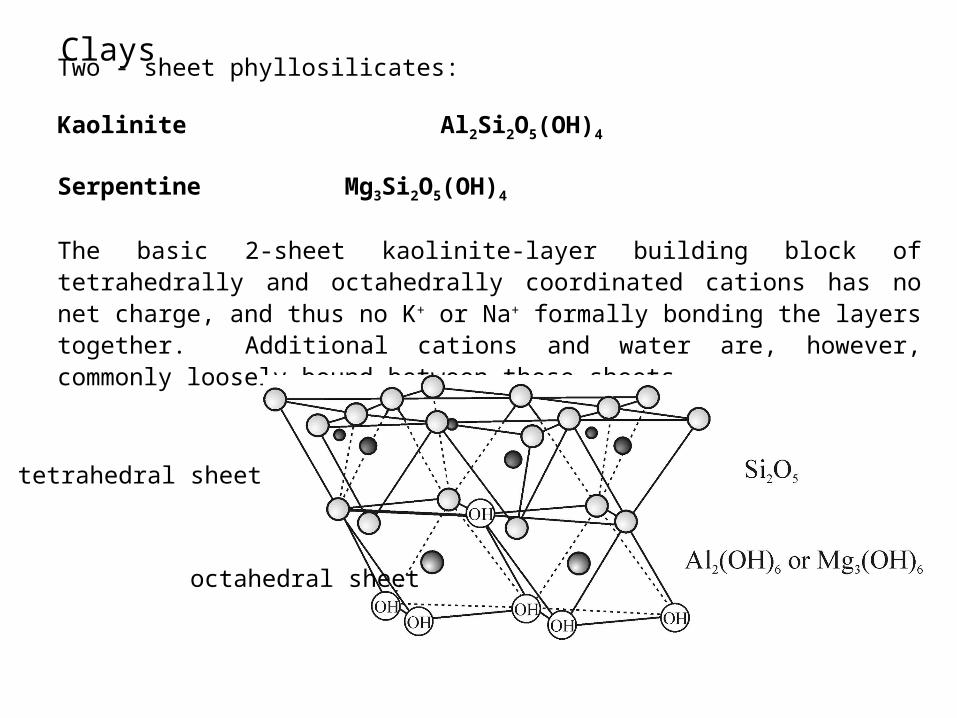
Two - sheet phyllosilicates:

Kaolinite Al2Si2O5(OH)4

Serpentine Mg3Si2O5(OH)4

The basic 2-sheet kaolinite-layer building block of tetrahedrally and octahedrally coordinated cations has no net charge, and thus no K+ or Na+ formally bonding the layers together. Additional cations and water are, however, commonly loosely bound between these sheets.

tetrahedral sheet

octahedral sheet

Clays

tetrahedral sheet

octahedral sheet

tetrahedral sheet

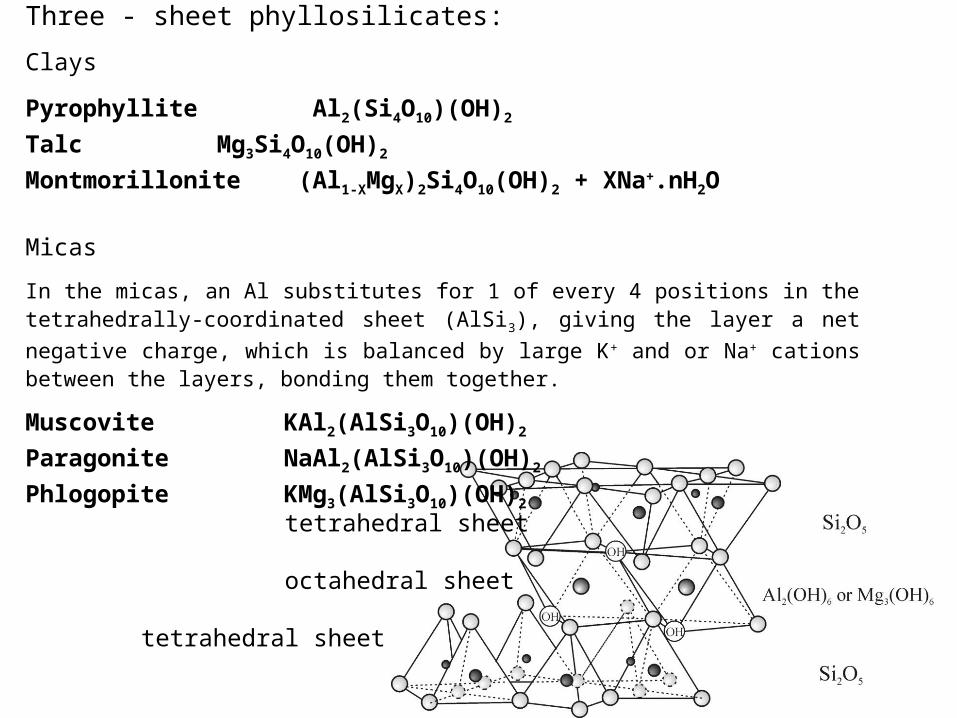
Three - sheet phyllosilicates:

Clays

Pyrophyllite Al2(Si4O10)(OH)2

Talc Mg3Si4O10(OH)2

Montmorillonite (Al1-XMgX)2Si4O10(OH)2 + XNa+.nH2O

Micas

In the micas, an Al substitutes for 1 of every 4 positions in the tetrahedrally-coordinated sheet (AlSi3), giving the layer a net negative charge, which is balanced by large K+ and or Na+ cations

between the layers, bonding them together.

Muscovite KAl2(AlSi3O10)(OH)2

Paragonite NaAl2(AlSi3O10)(OH)2

Phlogopite KMg3(AlSi3O10)(OH)2

Montmorillonite is a clay mineral that is intermediate between kaolinite and mica. Many of the weathering reactions we looked at previously form the clay mineral montmorillonite:

(Al1-XMgX)2Si4O10(OH)2-X + X×Na+.nH2O

as an intermediate step on the way to the formation of kaolinite. The substitution of some Al3+ by Mg2+ gives the octahedral sheet a negative charge, which is balanced by large low-valence cations such as Na+ and K+ between the sheets holding them together. Commonly kaolinite layers are intermixed with montmorillonite layers on a submicroscopic scale. The process of lithification involves the reverse reaction with a progressive gradation from two-sheet clay minerals to three-sheet micas with increasing temperature and pressure.

Montmorillonite

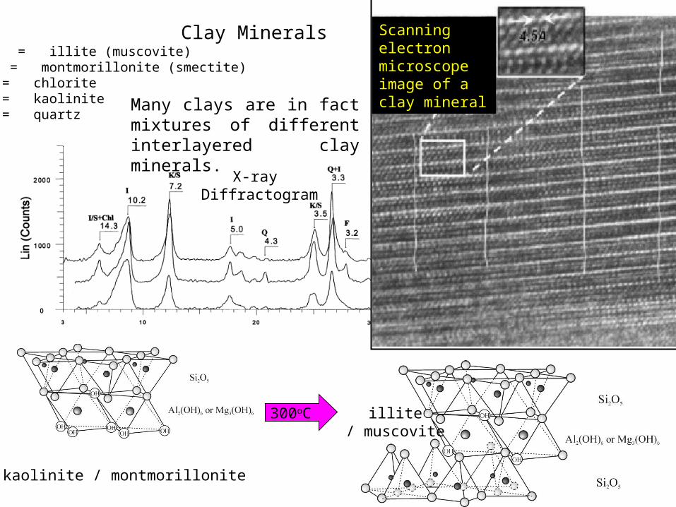
Clay Minerals

300oC

kaolinite / montmorillonite

illite/ muscovite

I = illite (muscovite)S = montmorillonite (smectite)Chl = chloriteK = kaoliniteQ = quartz

Many clays are in fact mixtures of different interlayered clay minerals.

X-ray Diffractogram

Scanning electron microscope image of a clay mineral

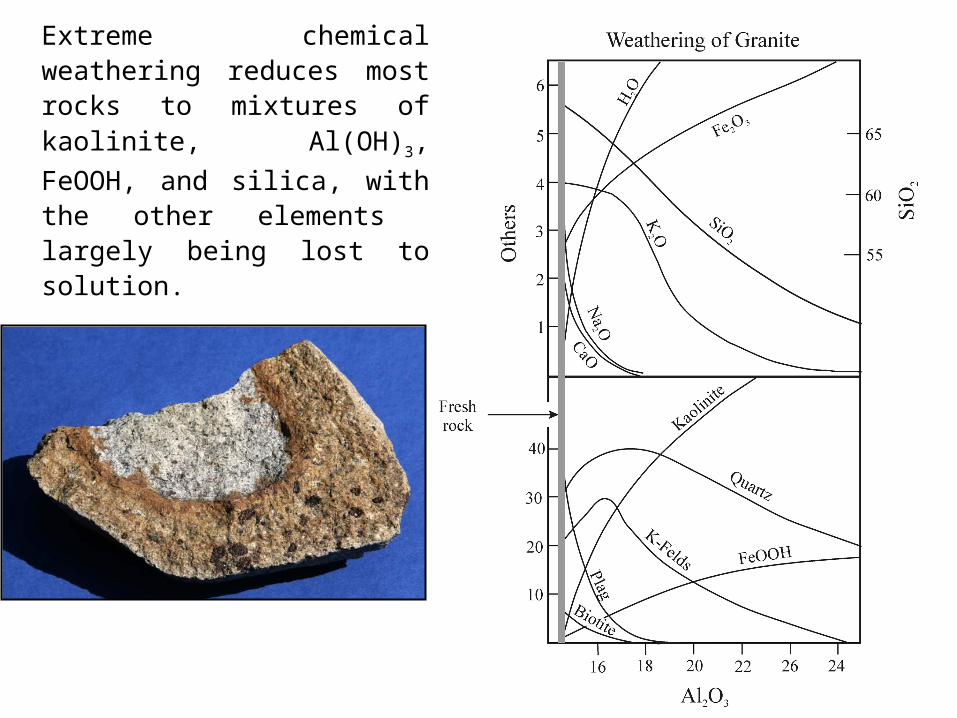
Extreme chemical weathering reduces most rocks to mixtures of kaolinite, Al(OH)3, FeOOH, and

silica, with the other elements largely being lost to solution.

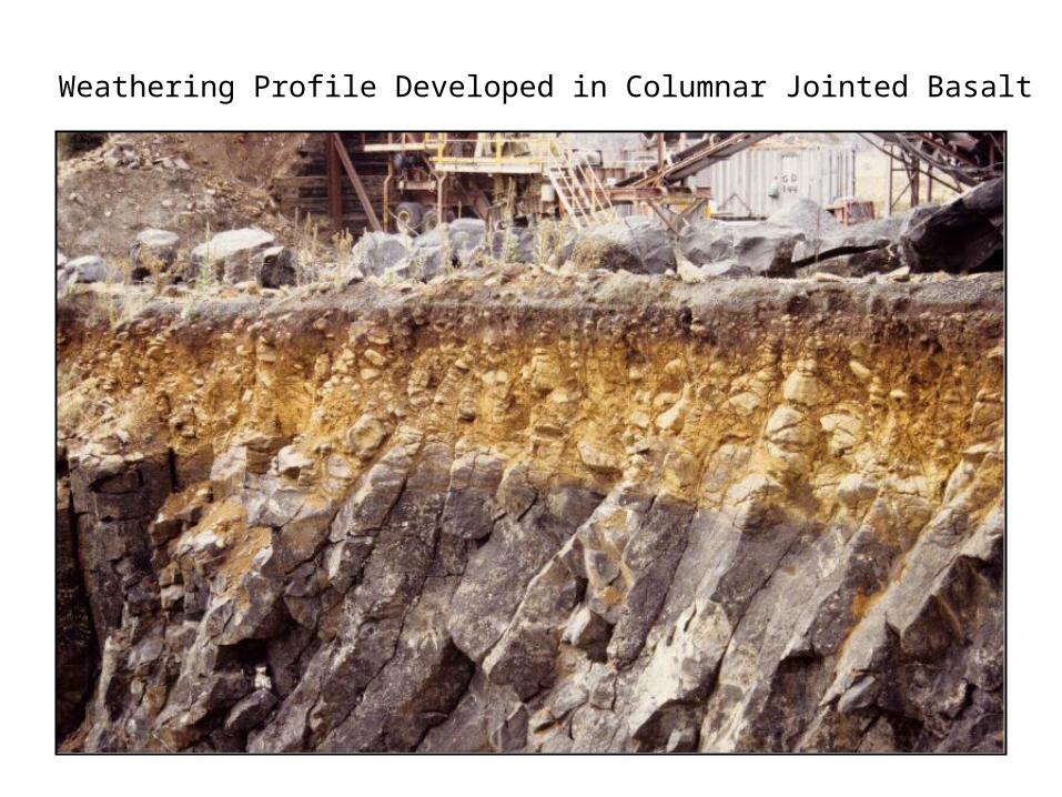
Weathering Profile Developed in Columnar Jointed Basalt

Parana Basalt

Saprolite %loss

MesozoicGranodiorite

Soil %loss

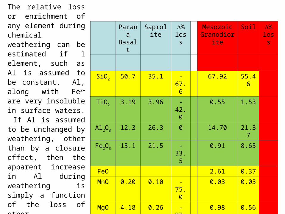
SiO2 50.7 35.1 -67.6 67.92 55.46

TiO2 3.19 3.96 -42.0 0.55 1.53

Al2O3 12.3 26.3 0 14.70 21.37

Fe2O3 15.1 21.5 -33.5 0.91 8.65

FeO 2.61 0.37

MnO 0.20 0.10 -75.0 0.03 0.03

MgO 4.18 0.26 -97.1 0.98 0.56

CaO 7.83 0.06 -99.6 2.94 0.38

Na2O 2.53 0.02 -99.6 3.31 0.49

K2O 1.71 0.13 -96.5 4.38 6.48

P2O5 0.46 0.11 -89.1 0.18 0.20

LOI 1.70 12.4 +240 1.16 4.55

The relative loss or enrichment of any element during chemical weathering can be estimated if 1 element, such as Al is assumed to be constant. Al, along with Fe3+ are very insoluble in surface waters. If Al is assumed to be unchanged by weathering, other than by a closure effect, then the apparent increase in Al during weathering is simply a function of the loss of other constituents.

Al2O3 :

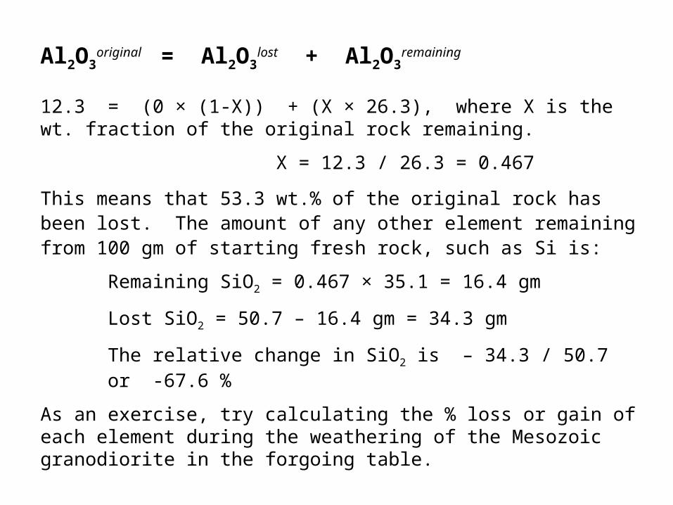
Al2O3original = Al2O3

lost + Al2O3remaining

12.3 = (0 × (1-X)) + (X × 26.3), where X is the wt. fraction of the original rock remaining.

X = 12.3 / 26.3 = 0.467

This means that 53.3 wt.% of the original rock has been lost. The amount of any other element remaining from 100 gm of starting fresh rock, such as Si is:

Remaining SiO2 = 0.467 × 35.1 = 16.4 gm

Lost SiO2 = 50.7 – 16.4 gm = 34.3 gm

The relative change in SiO2 is – 34.3 / 50.7 or -67.6 %

As an exercise, try calculating the % loss or gain of each element during the weathering of the Mesozoic granodiorite in the forgoing table.

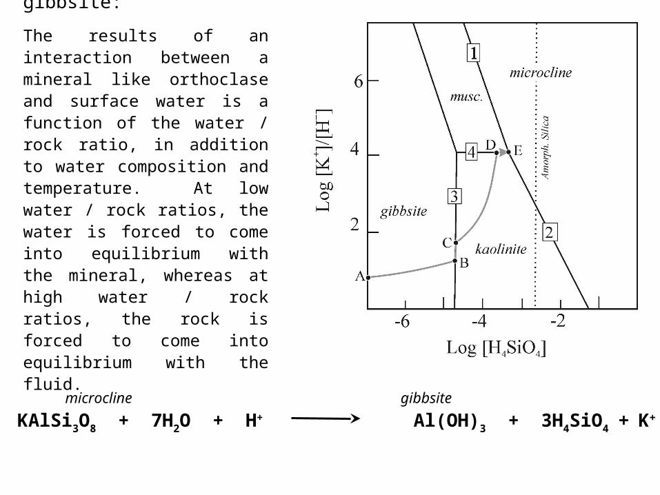
Chemical equilibria of the weathering of orthoclase to gibbsite:

The results of an interaction between a mineral like orthoclase and surface water is a function of the water / rock ratio, in addition to water composition and temperature. At low water / rock ratios, the water is forced to come into equilibrium with the mineral, whereas at high water / rock ratios, the rock is forced to come into equilibrium with the fluid.

KAlSi3O8 + 7H2O + H+ Al(OH)3 + 3H4SiO4 + K+

microcline gibbsite

Chemical equilibria of the weathering of microcline to gibbsite:

KAlSi3O8 + 7H2O + H+ Al(OH)3 + 3H4SiO4 + K+

2Al(OH)3 + 2H4SiO4 Al2Si2O5(OH)4 + 5H2O

2KAlSi3O8 + 9H2O + 2H+ Al2Si2O5(OH)4 + 4H4SiO4 + 2K+

3Al2Si2O5(OH)4 + 2K+ 2KAl3Si4O10(OH)2 + 3H2O + 2H+

3KAlSi3O8 + 12H2O + 2H+ KAl3Si4O10(OH)2 + 6H4SiO4 + 2K+

kaolinite

kaolinite

kaolinite

microcline

microcline

gibbsite

gibbsite

microcline

A to B

B to C

C to D

D to Emuscovite

If the amount of fluid is relatively small with respect to the amount of microcline, then the fluid will change composition as microcline is converted to gibbsite. In the extreme case of there being an infinite amount of microcline, the composition of the fluid will change to eventually come into equilibrium with microcline. At E, where orthoclase, kaolinite, and muscovite coexist, the Ph and K activity of the fluid are fixed or buffered by the mineral assemblage to constant values.

D muscovite

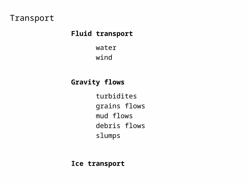
Fluid transport

water

wind

Gravity flows

turbidites

grains flows

mud flows

debris flows

slumps

Ice transport

Transport

Elementary Fluid Dynamics

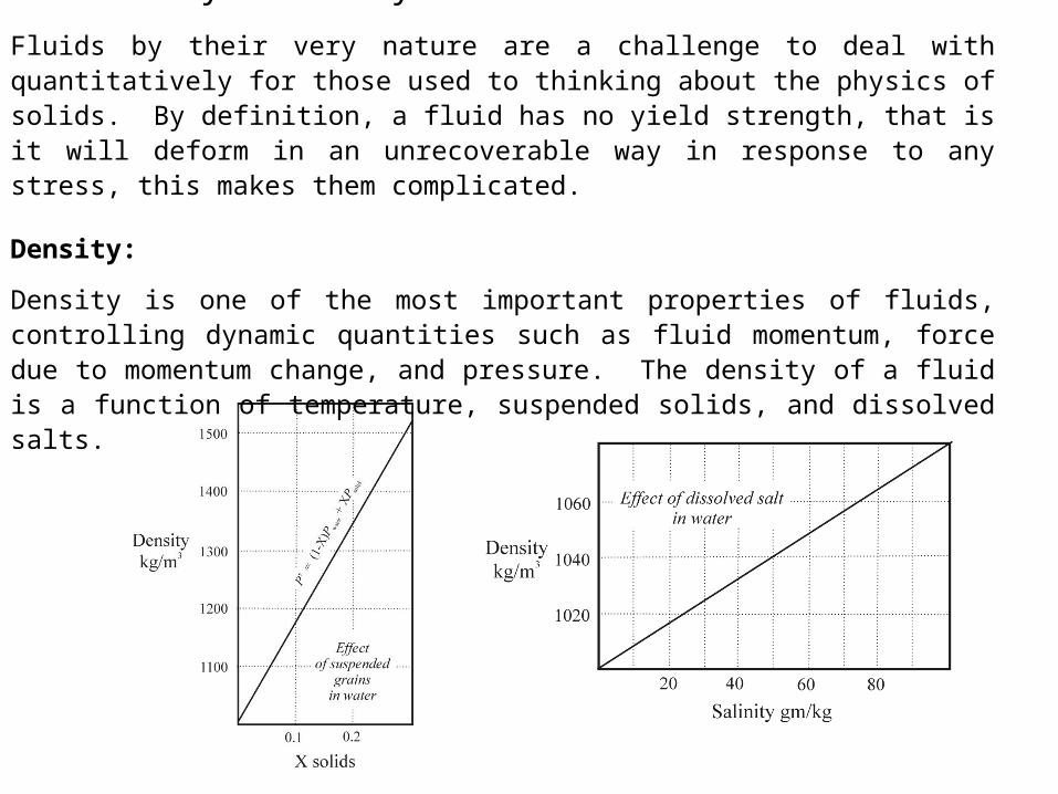
Fluids by their very nature are a challenge to deal with quantitatively for those used to thinking about the physics of solids. By definition, a fluid has no yield strength, that is it will deform in an unrecoverable way in response to any stress, this makes them complicated.

Density:

Density is one of the most important properties of fluids, controlling dynamic quantities such as fluid momentum, force due to momentum change, and pressure. The density of a fluid is a function of temperature, suspended solids, and dissolved salts.

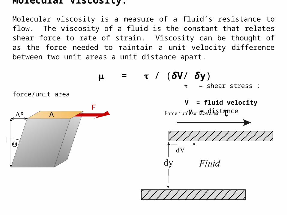
Molecular Viscosity:

Molecular viscosity is a measure of a fluid’s resistance to flow. The viscosity of a fluid is the constant that relates shear force to rate of strain. Viscosity can be thought of as the force needed to maintain a unit velocity difference between two unit areas a unit distance apart.

= / (δV/ δy) = shear stress : force/unit areaV = fluid velocity y = distance

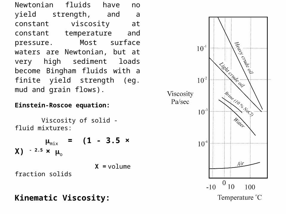
Newtonian Fluids

Newtonian fluids have no yield strength, and a constant viscosity at constant temperature and pressure. Most surface waters are Newtonian, but at very high sediment loads become Bingham fluids with a finite yield strength (eg. mud and grain flows). Einstein-Roscoe equation: Viscosity of solid - fluid mixtures: mix = (1 - 3.5 × X) - 2.5 × o

X = volume fraction solids

Kinematic Viscosity:

v = / = density

Dimensionless Parameters:

Four different forces are at play in fluid dynamics:

1) Gravitational forces proportional to g × ρ

2) Bouyancy forces proportional to g ×Δρ, due to the effect of gravity on differences in density.

3) Inertia forces proportional to V × ρ, due to the momentum of the current flow.

4) Viscous or retarding forces proportional to , due to viscosity or resistance to flow.

Many of the physical properties of fluid flow can be scaled in terms of dimensionless parameters that are effectively ratios of these four different forces.

Rayleigh Number:

The Rayleigh number is the ratio of buoyancy forces (α × ΔT × g × d3) to inertia forces (K × / ρ) :

Ra = (α × ΔT × g × d3) / K × / ρ

where: α = coefficient of thermal expansion K = thermal diffusivity d = depth ρ = density μ = viscosity

Fluids with Rayleigh numbers in excess of ~ 1000 will spontaneously undergo adiabatic convection. This also applies to solids that flow plastically such as the Earth’s mantle, and is responsible for the adiabatic melting that occurs in the upper mantle.

Reynolds Number:

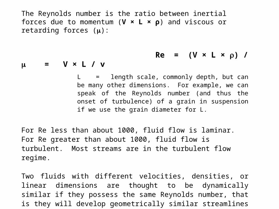
The Reynolds number is the ratio between inertial forces due to momentum (V × L × ρ) and viscous or retarding forces ():

Re = (V × L × ) / = V × L / v

L = length scale, commonly depth, but can be many other dimensions. For example, we can speak of the Reynolds number (and thus the onset of turbulence) of a grain in suspension if we use the grain diameter for L.

For Re less than about 1000, fluid flow is laminar. For Re greater than about 1000, fluid flow is turbulent. Most streams are in the turbulent flow regime.

Two fluids with different velocities, densities, or linear dimensions are thought to be dynamically similar if they possess the same Reynolds number, that is they will develop geometrically similar streamlines in the vicinity of geometrically similar objects.

Froude Number

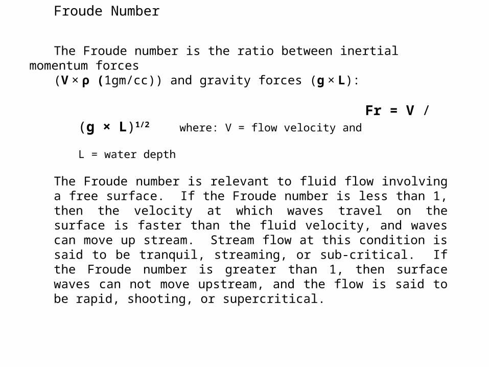
The Froude number is the ratio between inertial momentum forces(V × ρ (1gm/cc)) and gravity forces (g × L):

Fr = V / (g × L)1/2 where: V = flow velocity and L = water depth

The Froude number is relevant to fluid flow involving a free surface. If the Froude number is less than 1, then the velocity at which waves travel on the surface is faster than the fluid velocity, and waves can move up stream. Stream flow at this condition is said to be tranquil, streaming, or sub-critical. If the Froude number is greater than 1, then surface waves can not move upstream, and the flow is said to be rapid, shooting, or supercritical.

Bernoulli’s Equation:

½ (ρ × V2) + Ρ + (ρ × g × z) = constant kinetic flow gravitational energy pressure potential energy

Bernoulli’s equation is simply an expression of the conservation of energy for a flowing fluid. If the velocity increases, the resultant increase in kinetic energy is balanced by a decrease in flow pressure. Conversely if the flow velocity decreases, there is a corresponding increase in flow pressure. Among other things, this equation explains everything from the flow of water through pipes to how airplanes fly.

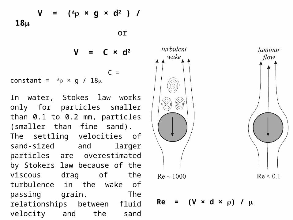
Stokes Law:

Gives the settling velocity for a spherical particle via laminar flow.

V = ( × g × d2 ) / 18 or V = C × d2

C = constant = × g / 18

In water, Stokes law works only for particles smaller than 0.1 to 0.2 mm, particles (smaller than fine sand). The settling velocities of sand-sized and larger particles are overestimated by Stokers law because of the viscous drag of the turbulence in the wake of passing grain. The relationships between fluid velocity and the sand transport capacity are better determined experimentally because of the theoretical complications of turbulent flow.

Re = (V × d × ) /

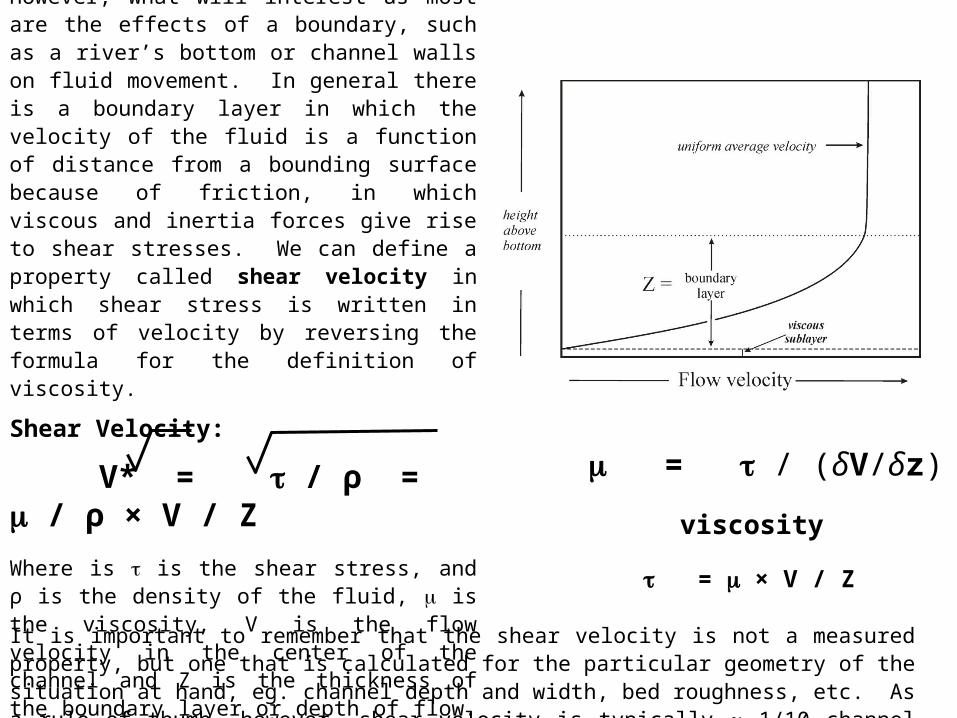
Boundary Layers:

Up until now, we have been dealing with fluids having no boundaries. However, what will interest us most are the effects of a boundary, such as a river’s bottom or channel walls on fluid movement. In general there is a boundary layer in which the velocity of the fluid is a function of distance from a bounding surface because of friction, in which viscous and inertia forces give rise to shear stresses. We can define a property called shear velocity in which shear stress is written in terms of velocity by reversing the formula for the definition of viscosity.

Shear Velocity:

V* = / ρ = / ρ × V / Z

Where is is the shear stress, and ρ is the density of the fluid, is the viscosity, V is the flow velocity in the center of the channel and Z is the thickness of the boundary layer or depth of flow.

= / (δV/δz)

viscosity

= × V / Z

It is important to remember that the shear velocity is not a measured property, but one that is calculated for the particular geometry of the situation at hand, eg. channel depth and width, bed roughness, etc. As a rule of thumb, however, shear velocity is typically ~ 1/10 channel flow velocity

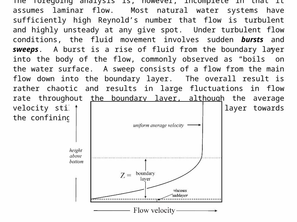
The foregoing analysis is, however, incomplete in that it assumes laminar flow. Most natural water systems have sufficiently high Reynold’s number that flow is turbulent and highly unsteady at any give spot. Under turbulent flow conditions, the fluid movement involves sudden bursts and sweeps. A burst is a rise of fluid from the boundary layer into the body of the flow, commonly observed as “boils” on the water surface. A sweep consists of a flow from the main flow down into the boundary layer. The overall result is rather chaotic and results in large fluctuations in flow rate throughout the boundary layer, although the average velocity still decreases across the boundary layer towards the confining surface.

Even under conditions of turbulent flow, however, there typically exists a viscous sub-layer across which flow is laminar, with a linear increase with distance. The thickness (~ 0.5 mm – 1 cm). of the viscous sub-layer is a function of the bed roughness and temperature. The colder the water and the larger the average grain size of the bed, the thicker the viscous sub-layer. Individual grains which protrude above the viscous sub-layer shed turbulent eddies and will experience much more fluid drag than grains that lie wholly within the viscous sub-layer.

viscous sub-layer

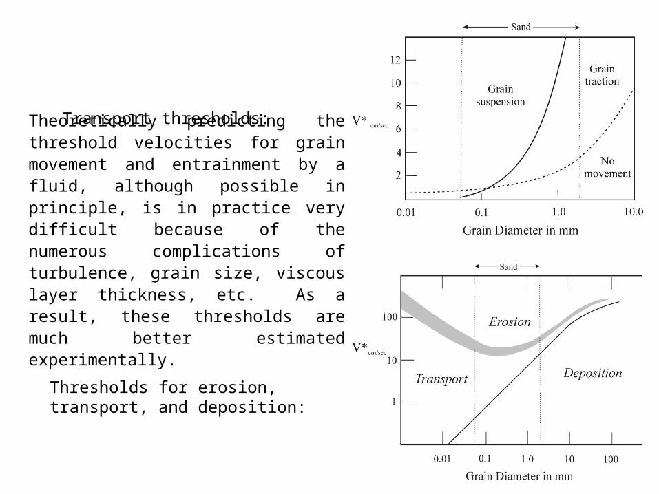
Transport thresholds:

Thresholds for erosion, transport, and deposition:

Theoretically predicting the threshold velocities for grain movement and entrainment by a fluid, although possible in principle, is in practice very difficult because of the numerous complications of turbulence, grain size, viscous layer thickness, etc. As a result, these thresholds are much better estimated experimentally.

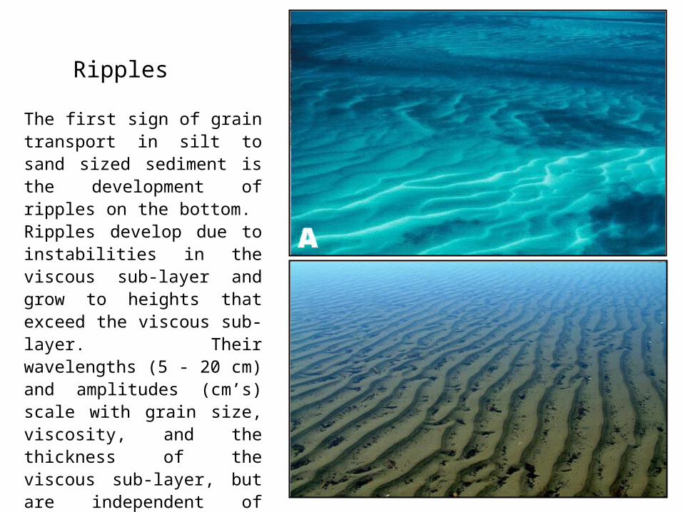
Ripples

The first sign of grain transport in silt to sand sized sediment is the development of ripples on the bottom. Ripples develop due to instabilities in the viscous sub-layer and grow to heights that exceed the viscous sub-layer. Their wavelengths (5 - 20 cm) and amplitudes (cm’s) scale with grain size, viscosity, and the thickness of the viscous sub-layer, but are independent of water depth.

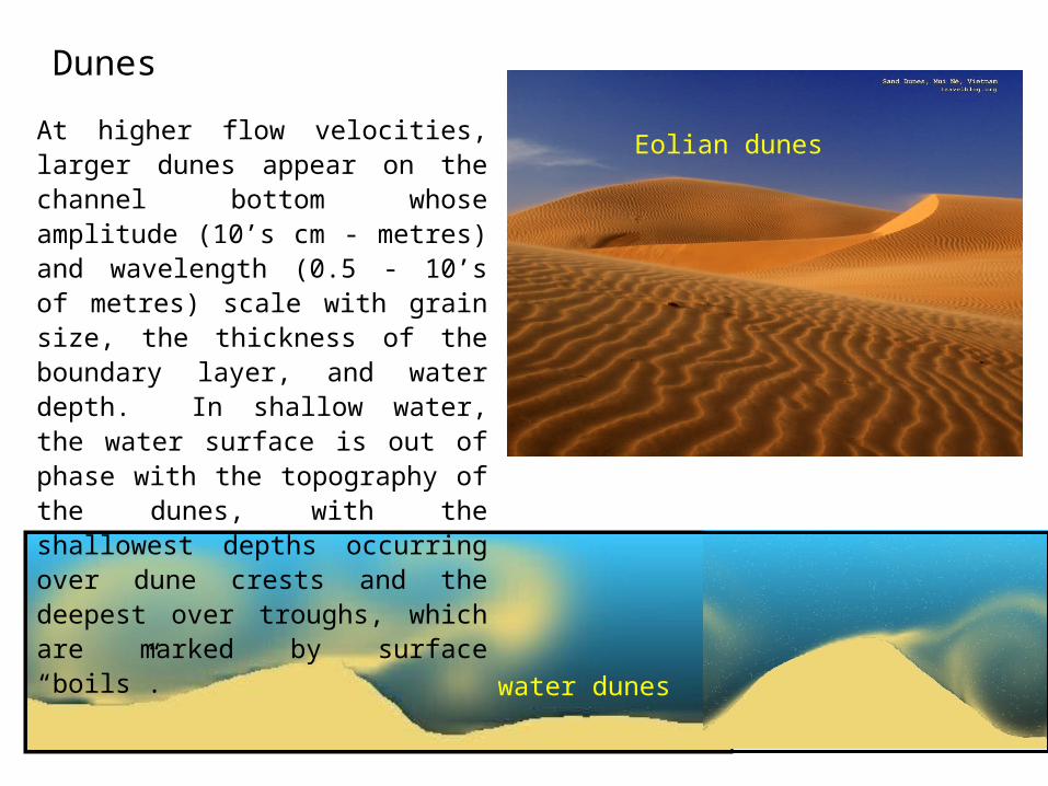
Dunes

At higher flow velocities, larger dunes appear on the channel bottom whose amplitude (10’s cm - metres) and wavelength (0.5 - 10’s of metres) scale with grain size, the thickness of the boundary layer, and water depth. In shallow water, the water surface is out of phase with the topography of the dunes, with the shallowest depths occurring over dune crests and the deepest over troughs, which are marked by surface “boils”.

Eolian dunes

water dunes

Bedforms

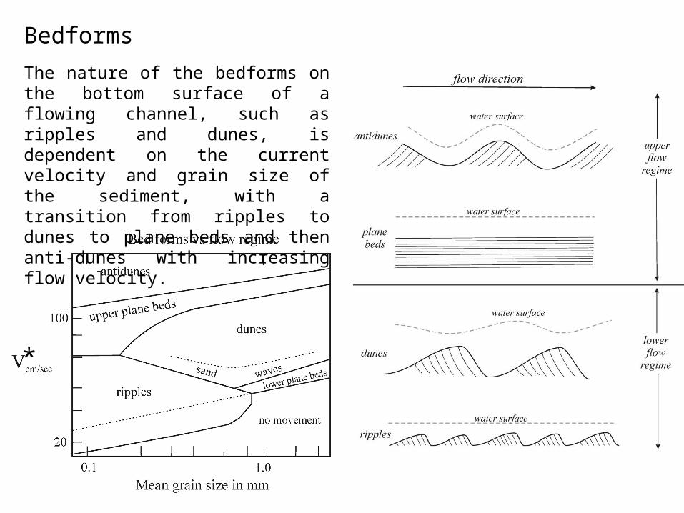
The nature of the bedforms on the bottom surface of a flowing channel, such as ripples and dunes, is dependent on the current velocity and grain size of the sediment, with a transition from ripples to dunes to plane beds and then anti-dunes with increasing flow velocity.

*

Plane laminations of the upper flow regime.

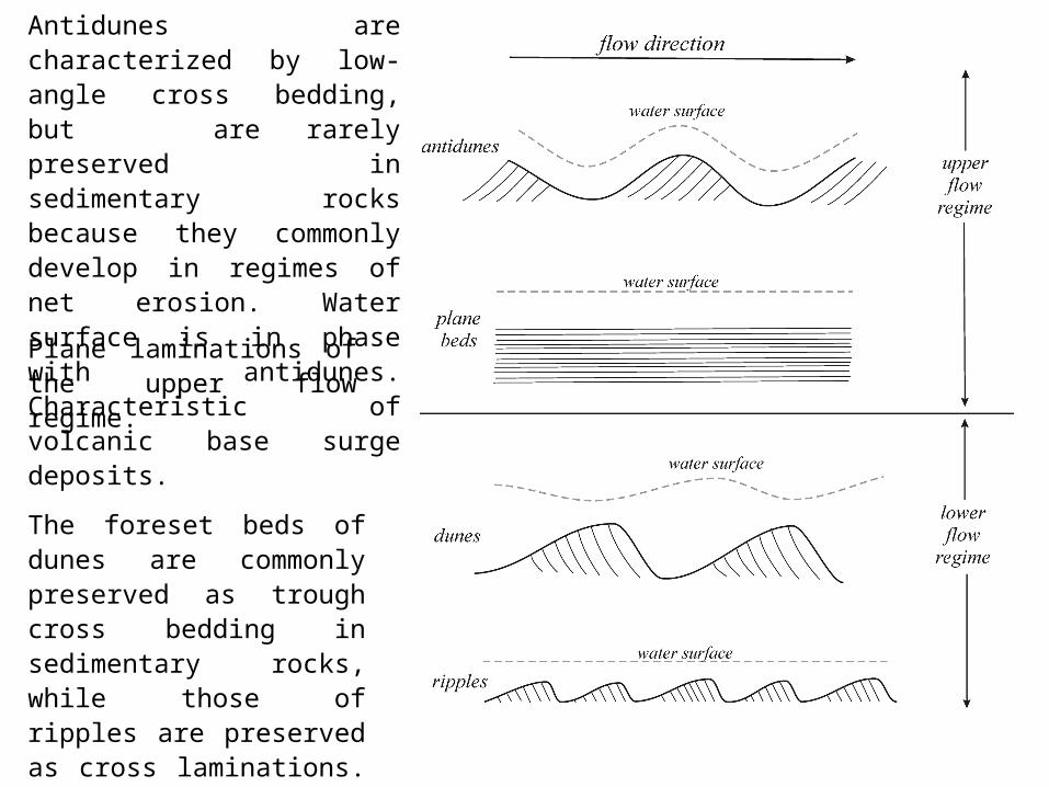
Antidunes are characterized by low-angle cross bedding, but are rarely preserved in sedimentary rocks because they commonly develop in regimes of net erosion. Water surface is in phase with antidunes. Characteristic of volcanic base surge deposits.

The foreset beds of dunes are commonly preserved as trough cross bedding in sedimentary rocks, while those of ripples are preserved as cross laminations. Water surface is out of phase with dunes.

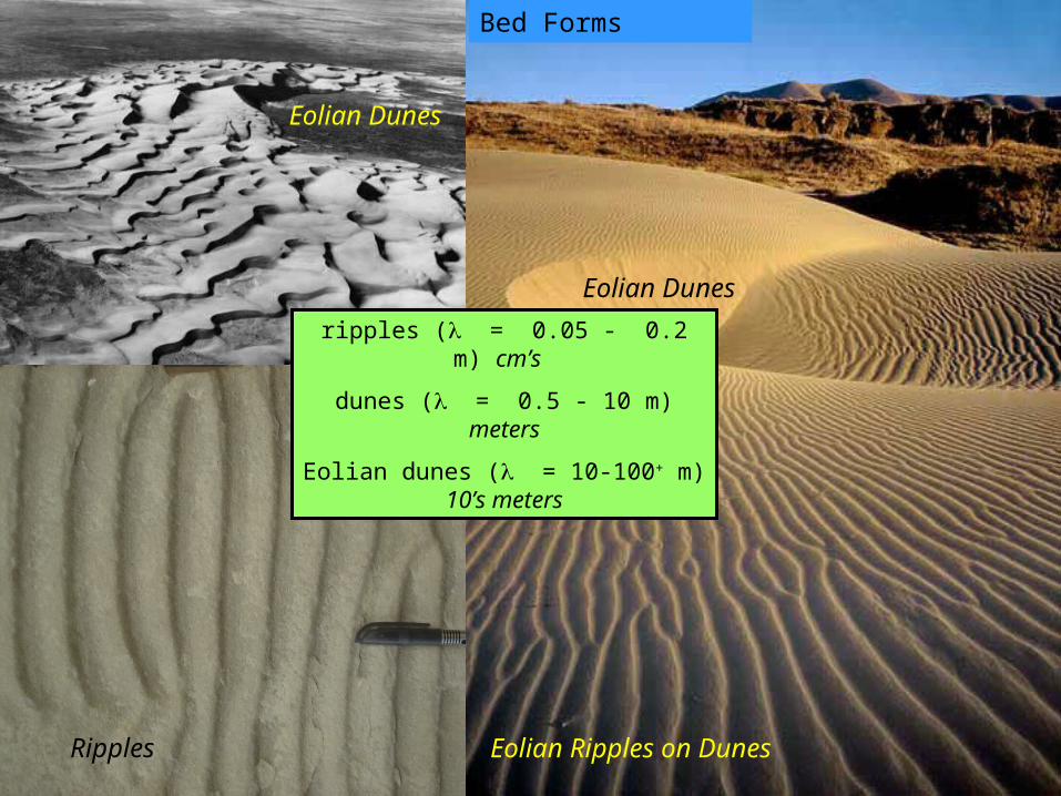
Bed Forms

Eolian Dunes

Eolian Ripples on DunesRipples

ripples ( = 0.05 - 0.2 m) cm’s

dunes ( = 0.5 - 10 m) meters

Eolian dunes ( = 10-100+ m) 10’s meters

Eolian Dunes

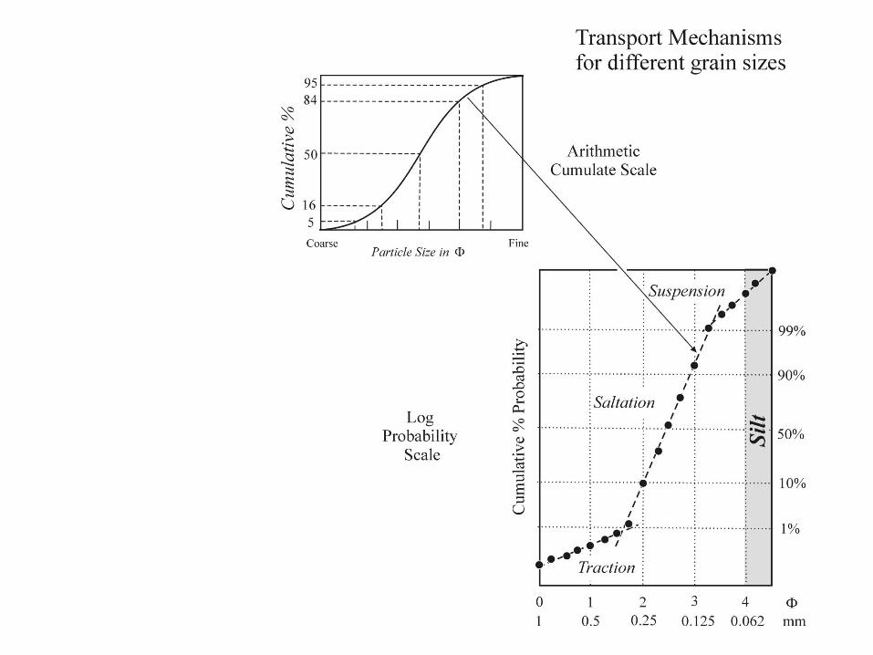
Grain-Size versus Transport Mechanism

There is a rough correspondence between the major grain size divisions and the transport mechanism, which is in return responsible for their physical separation during the fluid transport process.

• silts and clays are carried in suspension in the ‘wash load’

• sands are carried in ‘bed load’ by intermittent saltation and suspension

• pebbles and larger are carried in the ‘bed load’ by traction

Grain Size Statistics:

Sediment grain size distributions are determined using sieves of different hole sizes for fine sand to gravel and by measuring settling rates for clays to silts in water columns and using Stokes Law to determine grain size. The results are in weight units - that is the contents of each sieve are weighed to determine the weight portions of the grain size range caught by the sieves.

median = Φ50

mean = (Φ16 + Φ50 + Φ84) / 3standard = (Φ84 - Φ16) / 4 + (Φ95 - Φ5) / 6deviation

skewness = (Φ84 + Φ16 – 2Φ50) + (Φ95 + Φ5 – 2Φ50)

2(Φ84 - Φ16 ) 2(Φ95 – Φ5 )

kurtosis = (Φ95 – Φ5 )

2.44(Φ75 – Φ25)