General rights Copyright and moral rights for the publications made accessible in the public portal are retained by the authors and/or other copyright owners and it is a condition of accessing publications that users recognise and abide by the legal requirements associated with these rights.

Users may download and print one copy of any publication from the public portal for the purpose of private study or research.

You may not further distribute the material or use it for any profit-making activity or commercial gain

You may freely distribute the URL identifying the publication in the public portal If you believe that this document breaches copyright please contact us providing details, and we will remove access to the work immediately and investigate your claim.

Downloaded from orbit.dtu.dk on: Oct 19, 2021

SEE - Sight Effectiveness Enhancement. Results of the aeronautical evaluation

Andersen, H.B.; Alapetite, Alexandre

Publication date:2006

Document VersionPublisher's PDF, also known as Version of record

Link back to DTU Orbit

Citation (APA):Andersen, H. B., & Alapetite, A. (2006). SEE - Sight Effectiveness Enhancement. Results of the aeronauticalevaluation. Risø National Laboratory. Denmark. Forskningscenter Risoe. Risoe-R No. 1573(EN)

Risø-R-1573(EN)

SEE Sight Effectiveness Enhancement: Results of the Aeronautical Evaluation

Henning Boje Andersen, Alexandre Alapetite

Risø National Laboratory Roskilde Denmark

November 2006 Risø-R-1573

Author: Henning Boje Andersen, Alexandre Alapetite Title: SEE – Sight Effectiveness Enhancement, Results of the Aeronautical Evaluation Department: Systems Analysis Department

Risø-R-1573(EN) November 2006

ISSN 0106-2840 ISBN 87-550-3541-8

Contract no.: IST-2001-38228

Group's own reg. no.: 1225080-0010

Sponsorship: European Union Information Society Technologies Fifth Framework Programme

Cover :

Pages: 35 Tables: 3 References: 2

Abstract : The present report presents the deliverable D6.3 ‘Result of the Aeronautic Evaluation’ of the SEE project (“Sight Effectiveness Enhancement”, September 2002 – December 2005). Two parallel evaluations have been conducted: an experimental trial of the automotive and an experimental trial of the aeronautical application. The evaluations have measured the efficiency and HMI (human-machine interaction) characteristics of the SEE prototype. The evaluation of the aeronautic application was carried out in September 2005 in a fixed based simulator, emulating a Boeing 737 New Generation at THALES’ premises in Bordeaux, France. The simulator was equipped with a head-up display and the simulated environments specified and established in the project. The evaluation has involved as test subjects six professional 737 airline pilots. The document describes objective and subjective measures of performance. The analysis of results was completed in December 2005.

Risø National Laboratory Information Service Department P.O.Box 49 DK-4000 Roskilde Denmark Telephone +45 46774004 bibl@risoe.dkFax +45 46774013 www.risoe.dk

Risø-R-1573(EN) 2

Contents

1 Objective of the Aeronautic Evaluation 4

2 Experimental environment 4 2.1 The simulation environment 4

3 Experimental scenarios 5 3.1 Identification of parameters 5 3.2 Selection of scenarios 6 3.3 Specification of scenarios 6 3.4 Type of experimental design 7

4 Experimental subjects and briefing 8 4.1 Selection and recruitment of experimental participants: line pilots 8 4.2 Briefing and debriefing of participant pilots 8

5 Results 9 5.1 Limitations of the experimental environment 9 5.2 Results (A) – Approach/landing scenario Cat1 10 5.3 Results (B) – The take-off/runway incursion scenario 15 5.4 Results (C) – Pilots’ comments and recommendations 16

6 Conclusion 20

7 Acknowledgments 20

8 Appendix 1: Session Plan 21

9 Appendix 2: Bordeaux Experiments Geometry Methodology 23

Risø-R-1573(EN) 3

1 Objective of the Aeronautic Evaluation This document reproduces deliverable D6.3 for the European project SEE “Sight Effectiveness Enhancement” and describes the aeronautic evaluation of the enhanced vision system (SEE) that has been simulated and tested. The evaluation has been carried out in a fixed based simulator, emulating a Boeing 737 New Generation at THALES’ premises in Bordeaux. The simulator was equipped with a head-up display and the simulated environments specified and established in the project. The evaluation has involved as test subjects six professional 737 airline pilots. In this report, we describe objective measures (reaction times), expert instructor ratings of performance and subjective assessments elicited from the six pilots who had been involved as test subjects.

The overall goal of the aeronautical evaluation was to perform a test of the simulated SEE system that would have – as far as may be possible within the resources and time constraints of the evaluation task – a relatively high degree of credibility to experts (pilots, airline safety officers, aviation safety experts, regulators). To achieve this, it was decided (a) to involve as test subjects airline pilots who are type rated to the particular aircraft type that was implemented in the test simulator, and (b) to focus the tests on two types of risk scenarios associated with reduced visibility: approach and landing scenarios and runway incursion scenarios.

2 Experimental environment 2.1 The simulation environment The experimental environment in which the aeronautic evaluation was carried out was a fixed based-simulator facility set up at the premises of THALES in Bordeaux (Le Haillan). The simulator was set up to emulate the Boeing B737 New Generation, was equipped with controls and instruments and visuals for the left hand side (captain’s position): Primary Flight Display (PFD) and Navigational Display (ND), flight director controls and displays, control column and throttle box. The simulation of the flight environment and the flight dynamics (of the B737NG) were based on the X-Plane flight simulation software.

Risø-R-1573(EN) 4

Below, we list essential sub-systems specific to the SEE EVS simulation and the evaluation. We have sought to make the report short and do not duplicate technical information reported in other deliverables of the project. Please confer D7.4 for a technical description of the SEE EVS system and the simulation of this1.

- The simulator was equipped with a head-up display on which was shown (when selected and when supported) the EVS-data.

- EVS data were produced by the “fusion computer” supplied by Galileo-Avionica (confer D7.4) and projected onto the head-up display for the Pilot Flying (PF) in the captain’s position. The simulation of EVS-data is based on the models of the camera and the actual algorithm used for data fusion between data from the SWIR and LWIR ranges.

- The rendering of reduced visibility (fog conditions of varying density) was developed in the project (confer D7.4) and was overlaid on the “landscape” developed by OKTAL.

- The target airport and runway (Toulouse Blagnac, 32L) were modelled in a radius of 10 nautical miles from the threshold of 32L.

3 Experimental scenarios 3.1 Identification of parameters Based on the analysis and discussions reported in D6.1 (Plan for human factors evaluation)2, a further focusing on key parameters to assess during the aeronautic was made. The focusing was made necessary due to (a) the somewhat limited time the simulator would be available and (b) our decisions to use professional airline pilots (see next section) and the consequent restrictions on the time that these participants would be available.

The provisional list of parameters of to be assessed were:

Objective parameters - quantitative: reaction and detection times or distances. Safety limits and margins with respect to runway and other aircraft. Deviations from glideslope and localisers. Speed. Objective parameters – qualitative: blinded expert judgment rating: Ratings (assessments) of the safety of sections of flight as measured by flight experts / instructors are objective to the extent they are in so far as they are adequately “blinded”. In the context of expert assessment of flight safety on the basis of simulator performance, a “blind” assessment of performance refers to judges (instructors) who do not know whether a given flight was performed with or without the device (here: the SEE EVS) under evaluation. Subjective parameters as revealed by participants: pilot perception of safety gains, potential safety disadvantages or disadvantages in terms of, e.g., stress, workload, eye-strain.

1 SEE-deliverable D7.4, Final synthesis report 2 SEE deliverable D6.1, Evaluation plan for human factors evaluation

Risø-R-1573(EN) 5

3.2 Selection of scenarios The total time for which the simulator would be available was 4-5 days; this included configuration and scenario tests. For practical purposes, each crew would be available 5-8 hours. This was expected to allow for sufficient time for familiarisation and adequate execution of scenarios. Scenarios were selected on the basis of the following criteria:

- They should reveal potential safety gains as measured by objective measures – quantitative and qualitative.

- They should be representative of reduced visibility flight/ground situations that are recognised to be real and significant threats to aviation safety.

Based on these criteria and on the technical capabilities of the simulator, it was decided to implement an approach and landing scenario for each crew (run with and without the EVS) and a take-off / runway incursion scenario (similarly run with and without the EVS). In the selection and, in particular, in the composition of the scenarios, the experimental team received crucial assistance from a highly experienced B737 flight instructor.3

Two versions of the approach and landing scenario were prepared (at the lower limit of Cat1 and Cat2 minima, respectively), but implementation in the test simulator demonstrated that the Cat1 version of the this scenario would be – in terms of available visual cues – at the edge of what pilots would be able to cope with, being required to fly on “raw data” only.

The minima of the two visibility conditions are as follows:

Cat 1: the runway visual range4 at 200 feet above the runway shall be no less than 550 meters. Cat 2: the runway visual range at 200 feet shall be no less than 300 meters.

3.3 Specification of scenarios The specification of the scenarios (made with the indispensable assistance of the above mentioned flight instructor, who has extensive experience in planning, documenting and executing flight training scenarios) was modelled on standard proficiency scenarios used when training pilots for specific manoeuvres or procedures involving the use of specific cockpit resources.

Before the test scenarios were executed, an extensive familiarisation phase was to take place, during which pilots would familiarise themselves with the simulated aircraft, the controls and the rudimentary flight director, and the EVS system. The test scenarios were rehearsed – in order to eliminate “surprises”. While this may possibly appear to be “unrealistic”, it is in fact not an unusual way to train manoeuvres and procedures to pilots, and it is therefore also a customary way of rating pilot performance. It was decided to seek to eliminate in nearly all instances “surprises” to the test subjects – for several reasons. A chief reason was that we wanted to compare performance on the same scenario flown with and without the EVS. Evidently, a surprise element cannot be used twice for the same crew unless there are alternatives.

3 Captain Steen Andersen, Maersk-Air/ Sterling. 4 Runway visual range (rvr) is a technical term that does not quite correspond to the range at which a normal sighted person can

see an unilluminated object. In the implementation of the visibility ranges we have used the rule of thumbs that pilots sometimes use if they have no other information: centre lights and runway lights shall be visible at the distances quoted in the definitions cited of Cat 1 and Cat 2. Standard distance between runway lights is 200 feet or roughly 60 meters. So for Cat 1 conditions, if one is positioned in the cockpit a few meters above the runway, 9 lights should be visible, and for Cat 2, 5-8 lights should be so.

Risø-R-1573(EN) 6

Scenario 1: the approach and landing scenario implemented as a visibility condition of Cat1 (bordering on a Cat2). The crew would be initiating the scenario at 3000 feet, 8 miles from the target runway. See next section under “Briefing” where the instructions describe the flight and aircraft configuration details. The crew was instructed to continue approach and land on the runway (32L at Blagnac). The scenario would be run with or without the EVS; in both versions, it would be the same reduced visibility conditions that would be engaged, namely uniform fog that would allow, at 200 feet above the runway, a visibility of 550 m. Scenario 1 would be run in two trials for each pilot, hence four trials for each crew. See Appendix 1 where the experimental plan is reproduced. Pilots were instructed that go-around was not an option – that they had to land due to “uncontrollable fire and smoke in cabin”.

Pilots’ comment on the implementation of the scenario was that it resembled a Cat2 rather than a Cat1 scenario.

Scenario 2: the take-off/runway incursion scenario. This scenario involved a take-off at full thrust during Cat 2 conditions. At a fixed distance, an incursion aircraft is placed on the edge of the runway, with lights on and having its wing extending into the runway. All take-offs are initiated at the same position. The aircraft becomes visible with the EVS engaged at around 60-70 knots (around 400 m before the incursion aircraft), and without the EVS at around 80-90 knots (around 180 m before the incursion aircraft). The placement of the aircraft is randomly changed from the left and the right side of the runway; hence the pilot flying will not know at which side the incursion airplane would appear. Nor will pilots be told at which distance (speed) the aircraft might be visible.

3.4 Type of experimental design As will be detailed in the next section, it was decided to recruit 6 pilots divided into 3 crews. The experimental design was based on the so-called within-group (or repeated-measure) design, which at the same time allows the use of within-group (repeated-measure) statistical tests. Results from a within-group design (in contrast to a between-group design) may therefore (provided other conditions are met) be tested for statistical significance by relatively powerful (sensitive) tests. These tests have greater power than between-group tests, since the variation within a group (the variation between individuals) can be eliminated when we compare the same individual under two conditions. For instance, there may be large individual differences between the pilots for some tasks, whereas when we measure each pilot under two conditions, we may discount the variation within the group. In order to eliminate possible systematic effects of the order in which the two conditions are engaged (with and without the EVS), this must be balanced evenly across trials.

The specification of the scenarios (made with the essential assistance of the above mentioned flight instructor, who has extensive experience in planning, documenting and executing flight training scenarios) was modelled on standard proficiency scenarios used for training pilots for specific manoeuvres or procedures involving the use of specific cockpit resources. See next session.

Risø-R-1573(EN) 7

4 Experimental subjects and briefing 4.1 Selection and recruitment of experimental participants: line pilots It was decided at an early phase of the project that it would be desirable to have the aeronautic application evaluated by involving professional airline pilots as test participants. The rationale for choosing professional type-rated pilots as test “subjects” – rather than, say using volunteer or student subjects – is that the evaluation may thereby gain a higher degree of credibility. That is, the evaluation will thereby be able to involve realistic tasks that are worked at by “real” users in a reasonably faithful task environment (the simulation environment).

In total, six pilots divided into three crews were recruited for the experiments. Four pilots from Maersk-Air (later Sterling) and two pilots from Thomson (airline): three pilots were captains, and three were first-officers. All pilots were type-rated to the B737 New Generation and all of them were flying a full time schedule.

Pilots received a monetary compensation for their participation covering their preparation, travel to and from Bordeaux and participation in the trials.

4.2 Briefing and debriefing of participant pilots The verbal instructions to the pilots followed the following written instructions. These were given to pilots the evening before their day of experimental evaluation.

Due to the limitations of the test simulator, your primary flight display will be configured as follows:

• No FD / flight director • No minima bug (RAM) • Stick shaker deactivated • PFD only in left side • PNF makes call-outs from PFD

Flying must be based on “raw data” only!

1. Familiarization trials. You will make a take-off, a low overflight, and then a couple of approaches and landings with the EVS (Enhanced Vision System).

After this, we go to the actual test scenarios: a Cat 1 approach /landing, and a take-off in Cat 2 conditions.

2. For the approach / landing scenarios

We reposition you at: final on RWY 32L, Blagnac:

• Repositioned at 3000 feet on final RWY. 32L • Vref. Flaps 40 = 150 kt • All tests are emergency landings - go around is not an option • Engage autopilot • Autothrottle on • Course selectors: 325, and Heading: 325 • Select VNAV and LNAV • Fully configured pitch attitude at 3.5-4 degrees nose up • N1 = 65%

Risø-R-1573(EN) 8

Then release simulator / aircraft. When released, the aircraft will gradually catch localizer and glideslope. When released, the aircraft will tend to pitch down to the left or right. Throttle handles not yoked because of faulty magnet.

At approximately 3000 feet altitude, disengage autopilot

• Final speed 140-150 kt • Apply speed brake manually

3. Instructions for take-offs:

• Parking brake set • Apply thrust (Firewall) • Release parking brake

Recall, please: the goal of the evaluation is not to test pilot performance. And in any case, the simulator is so limited in features that it would not make sense to do so. The goal is:

(a) To compare performance with and without the Enhanced Vision System (b) To obtain experienced line pilots' assessment of advantages and disadvantages of the current

prototype Thank you for your efforts!

After the trials were concluded, each crew was debriefed: this involved an interview during which pilots were asked to comment on their experience with the (simulated) EVS. Subsequently, pilots were asked to fill out a questionnaire. The questions asked during the structured interviews and the items of the questionnaire are contained in the Results sections below.

5 Results 5.1 Limitations of the experimental environment The simulation environment was severely limited in several respects, as described briefly above and as mentioned in the briefing to pilots. The limitations which affect the approach and landing scenario were in particular the following: rudimentary flight director, a tendency to nose pitch-up, an illusion that one was seated higher above the ground – and more importantly: difficult to distinguish background and objects on the HUD screen on which the simulated EVS data are projected. In addition, one pilot using progressive glasses was not able to use the EVS in a useful way. These difficulties have to be mentioned because they have an impact on the results. The problems with controlling the aircraft were the same, of course, whether or not the EVS was engaged. However, the control problems were particularly acute when pilots had no visual cues and had to fly by “raw data” only – by the dots of the localiser indicator and the glideslope indicator in effect. The difficulties we have mentioned therefore impact on the results in two ways: first, the potential advantages of the EVS become dampened, especially by the HUD problems; second, the difficulties (even in a “well-behaved” full flight simulator) of flying on raw data only introduce random error and therefore noise into the data. These difficulties pertain to the approach and landing scenario mainly, while the take-off/incursion scenario execution was only affected by difficulties in exploiting the visual cues of the HUD.

Risø-R-1573(EN) 9

5.2 Results (A) – Approach/landing scenario Cat1 The landing scenario was executed (in test conditions) four times for each of the six pilots, twice with and twice without the EVS. This yields twelve pairs of trials, two pairs for each pilot. A pair of trials thus consists of two consecutive trials carried out by the same pilot, one trial being with and one without the EVS. One of the trials had to be discarded due to interaction between the HUD and glasses of the pilot. This leaves us therefore with 11 pairs to be evaluated.

The data from the simulator log were processed with the purpose of enabling the Risø team to generate charts that instructors use when they assess the safety of landings performed by pilots in a full flight simulator or alternatively, when instructors want to document to pilots where and how they may have deviated from safety minima.

Instructors use essentially three types of data charts:

- actual glideslope/deviation from prescribed glideslope

- localiser deviation

- speed chart

Risø-R-1573(EN) 10

In Appendix 2, we describe in details how we have generated the charts based on the simulator logs. The glideslope and the localiser (centre line) deviation charts are reproduced above.

In order to assess the 11 pairs of landings, two senior and highly experienced pilot instructors5 helped us and acted as expert judges in a “blind” rating session. The two judges were each and independently presented with 11 pairs of sets of charts. Each pair comprised, as described above, two landings made by one and the same pilot, one landing with and one without the EVS. For each landing, there were the above mentioned three charts, though it was primarily the glideslope and the localiser deviation charts that were used. The judges did not know which of the landings of a given pair was with the EVS. The task given to the two instructors was to indicate which of the two landings of any given pair was safer (much safer or slightly safer) than the other or possibly, if the two landings were equal in safety. See table 1, where we reproduce the ratings of both judges.

5 In addition to Captain S. Arnesen, we profited from the expertice of Captain Finn Helbo.

Risø-R-1573(EN) 11

Table 1

Please judge each pair of landings in terms of safety

Session pair number

A much better than B

A slightly better than B

A and B are the same

B slightly better than A

B much better than A

Pair no. 1 1 1 Pair no. 2 2 Pair no. 3 1 1 Pair no. 4 1 1 Pair no. 5 1 1 Pair no. 6 1 1 Pair no. 7 1 1 Pair no. 8 1 1 Pair no. 9 1 1 Pair no. 10 1 1 Pair no. 11 2

The pilot instructors agree for 10 out of the 11 cases about which of the two flights in any pair is the safer. Their agreement about the degree of difference – whether one is “much better” or “slightly better” than the other – is not very high, in contrast. Only for pairs no.2 and no.11 do they agree about the degree, but they disagree in the remaining 9 cases. Still, it is the agreement about which landing is the safer that we need to compare to the actual configuration of the simulator.

Risø-R-1573(EN) 12

In order to compare the rating by the instructor judges to the actual state of the system (the EVS-status: engaged or not engaged), we first combine the ratings by the two pilot instructors. As we have noted, they agree on which landing is the safer in 10 cases and disagree in only case (session pair number 1).

Table 2: comparing instructors’ joint rating against actual EVS- status of the landings in each pair of landings

Consensus rating: which landing is the

safer of a given pair?

In which of the two landings was the EVS engaged?

Pair no. 1 Judges disagree B

Pair no. 2 A * B

Pair no. 3 A A

Pair no. 4 A A

Pair no. 5 B B

Pair no. 6 A A

Pair no. 7 B B

Pair no. 8 A A

Pair no. 9 A * B

Pair no. 10 B B

Pair no. 11 A A

In Table 2, we have aligned the consensus rating by the two instructors and the actual state of the system (EVS-status): whether it was the A or the B landing that had the EVS system engaged. We can see that the joint rating by the judges succeeds in identifying the EVS-engaged landing in 8 out of 10 cases: For pairs number 2 and 9, the judges assess the landing without the EVS as being the safer of the pair.

The question we now need to answer is this: is the instructors’ consensus judgment about which of the landings is the safer significantly correlated with the EVS-status? I.e., is there a significantly greater likelihood that the EVS was engaged for a given landing whenever the instructors’ agree that the landing was the safer?

The raw “success rate” is 8/10 or 80%. However, by pure chance, the chance of agreement would be 50%. So, if we take the chance element into account, the agreement is not so impressive perhaps. But this overlooks the chance element and if we take this into account the agreement is not so impressive. There is, however, a statistical test – Cohen’s kappa - that can be used and is customarily used to assess the degree of agreement between independent judges. Cohen's kappa is a chance-corrected measure of inter-rater reliability that assumes two raters, n cases, and m mutually exclusive and exhaustive nominal categories.

Risø-R-1573(EN) 13

The formula for calculating kappa is:

k = (Fo - Fc) / (N - Fc) Where: N = the total number of judgements made by each coder, Fo = the number of judgements on which the coders agree and Fc = the number of judgements for which agreement is expected by chance.

When computing kappa, the output is a number ranging from -1.0 to +1.0 (or from -100% to +100%). A kappa value of zero indicates that there is no agreement above chance; a negative kappa values obtains when the observed agreement is less than could be expected by chance. The interpretation of which levels of kappa may be regarded as less than acceptable agreement is necessarily a matter of convention. However, an often cited source [source Landis and Koch 1977] suggests the following levels as benchmarks (Table 3).

Table 3

Kappa Value Conventional interpretation: Agreement / correspondence is…

0.00-0.20 Slight

0.21-0.40 Fair

0.41-0.60 Moderate

0.61-0.80 Substantial

0.81-1.00 Almost perfect

When calculating the kappa value of comparing the joint assessment by the two instructors against the true state of the system (plus or minus EVS), we obtain the following result:

Kappa = 0.60 – or sixty percent chance-corrected agreement (SPSS 13.0) Significance - p-value = 0.038 Thus, although there are few data and although simulator problems have introduced a large amount of noise into the results, it has turned out that two independent judges picking out the safer flight of any pair show a moderate-to-substantial correlation with the flight being executed with or without the EVS

Risø-R-1573(EN) 14

5.3 Results (B) – The take-off/runway incursion scenario The data from this scenario were also depleted due to in part simulation problems and in part problems with the HUD interacting with glasses.

For each pilot, we intended to collect data from two take-off sessions, one with and one without the EVS. Data from one pilot were corrupted and from another we had the aforementioned suspected interaction with progressive glasses.

The remaining eight data points (four pairs) are displayed in the chart below, where we show the distance in meters to the runway incursion aircraft at the time when the pilots own aircraft starts to be retarded. We have already mentioned the power of within-group statistics, and this is well illustrated by calculating the difference between the rejected take-offs with and without the EVS. Using the paired sample t-test, we obtain a very high level of significance – p<0,00008 (one sided test; SPSS 13.0). At the same time, the size of the difference is also impressive: the average difference being 401 meters (max: 433 m; min: 361 m).

Time of reaction: meters before RWY incursion obstacle

0

50

100

150

200

250

300

350

400

450

500

1 2 3 4Crew number

Met

ers

befo

re o

bsta

cle

EVS+ EVS-

Distance of reaction With EVS Without EVS Difference = safety gain

Max 433 meters 204 meters 247 meters

Min 361 meters 144 meters 202 meters

Mean 401 meters 179 meters 222 meters

Risø-R-1573(EN) 15

5.4 Results (C) – Pilots’ comments and recommendations The crews were interviewed after their trials about their reactions to and comments and suggestions about the EVS. One crew submitted written comments subsequently. In the first part of this section, we review pilots’ comments and in the second part, we present pilots’ responses to a questionnaire they were given.

Comments from structured interview/debriefing or submitted in written form:

1. What was your immediate reaction to the EVS?

Responses:

It will offer massive gains in situation awareness.

Especially good for ground navigation and runway incursions.

The idea is good – but the simulator setup had drawbacks. Too narrow field of vision. The green background glare very annoying for normal vision.

All pilots noticed that the video monitor in the first officer’s side showed a much better quality picture than on the HUD.

Some pilots commented on the flight director on the HUD – wanted / suggested numeric heading information.

It was surprising that the EVS gave the impression (illusion) of a steeper approach. But the simulator might be to blame.

Hard on your eyes for extended periods – which pilots recognised would not be relevant for intended use of the EVS/HUD.

Suggested TCAS on the HUD as well on ground.

2. In your opinion, what are the most important gains of the EVS? Please comment on the following four phases: (a) Taxi; (b) Takeoff; (c) Approach; (d) Landing.

Responses:

b. Takeoff. This is properly the phase were there is most gain. As a low visibility takeoff is quite hairy. Here the EVS gives an early warning of obstacles ahead. You just need to learn to interpreted visual clues, as they are different from normal visual clues

c. Approach – no gain

d. Landing. Opinions are divided: one pilot finds no gains for app/landing, the other pilots think there are gains, two that there are definite gains (Cat 1 and 2 – don’t know how it will work under Cat 3 conditions).

Risø-R-1573(EN) 16

3. In your opinion, what are the most important disadvantages of the EVS? Please comment on the following four phases: (a) Taxi; (b) Takeoff; (c) Approach; (d) Landing.

Responses:

General: Concern that colours of light are not visible, that for instance the PAPI lights (red/green) are not recognisable. One pilot “colour is very crucial – hope it can be solved”.

General: Criticism of the “background noise” on the EVS-picture on the HUD in the prototype – too hard to adjust

c. Approach. I had trouble in the approach phase due to multi-focal glasses, and due to the simulator flying at a too high pitch attitude. The system will have to have a very well calibrated adjustment system, as the pilot must be sure he will receive the same level of visual input in all aircrafts. There is no time to adjust the system during approach.

d. Landing no gain, it is annoying during flare; maybe during landing roll it could have some advantage in low visibility takeoff.

4. In your opinion, what types of information (lamps, runway edge, marks, other aircraft, objects, terrain) should be captured during the four phases: (a) Taxi; (b) Takeoff; (c)

Approach; (d) Landing.

Responses:

a. Taxi. Taxi lights, aircrafts and vehicles

b. Take-off. Runway lights, aircrafts and vehicles

c. Approach. Approach and runway lights

d. Landing. Runway lights, aircrafts and vehicles

5. Please give us your recommendations for improving the EVS?

Responses:

Would be useful to have a calibration system with fixed values.

Remove background glare / reduce noise – compare the first-officer’s video display

A broader field of vision might be useful.

It would be useful to have a test picture to help with calibration before you need the HUD – it is definitely too late to adjust the display (background/ noise) when you need it.

One pilot suggested trying other colour than green on the HUD (amber?)

One pilot suggested options for turning on and off symbology (parts of symbology) on the HUD, e.g., option for switching between numerical or only analogue heading information.

Risø-R-1573(EN) 17

6. How would you like information to be displayed? Please comment on the four phases: (a) Taxi; (b) Takeoff; (c) Approach; (d) Landing.

Responses:

Present presentation is good though with the problems mentioned above

No other comments / preferences expressed

7. What would you like to be able to adjust and select and de-select on the EVS? (For instance, the HUD or the head-down view? Field of view? Contrast? Brightness? Other?)

Responses:

Independent adjustment of brightness and contrast.

A switch on controls to turn the system off, with out moving hands away from control column.

8. Is it important, and if so, how important is it that (a) both pilots have the EVS available, and (b) have it available at the same time?

Responses:

If the objective is to allow landing in lower minima and increase safety, it is very important that both pilots have the system available simultaneously.

Extremely desirable that both pilots have the system, especially during app/landing.

If only one pilot has the system. The other pilot is out of the loop – this should be avoided.

Risø-R-1573(EN) 18

Questionnaire responses:

The questionnaire responses supplied by the pilots (one was lost, possibly in the mail) are provided below:

To a very

RESULTS – responses from five pilots Not at all small

degree

To some degree

To a large degree

To a very large degree

1. General Issues

How confident were you in the terrain information conveyed by the display? 3 2

Did the infrared picture always provide a clear picture of the environment? 2

0,5 “In air”

2 0,5 “ground”

3. Terrain Features: To what degree…

... could you distinguish terrain features with the EVS in general? 2 2 1

... could you distinguish between the runway and the grass with the display? 3 2

... could you see the runway edge lines with the display? 3 1 2

... could you see the runway centre-lines with the display? 3 2

... could you see the runway lights with the display? 2 3

... could you see touchdown zone with the display? 2 1 1

4. Approach / landing; take-off: To what degree does the EVS improve the safety of…

… a visual approach in CAT 1 conditions, no ILS? 4 1

… a visual approach in CAT 2 conditions (emergency - no ILS)?

3 1 1

… a take-off in CAT 1 conditions? 1 1 1 2

… a take-off in CAT 2 conditions? 2 3

To what degree are you able to estimate distances reliably with the display? 4 1

To what degree are you satisfied with the field of view of the display for carrying out the take-offs and landings? 1 2 2

To what degree did you find it necessary to look outside – or around - the display during approach? 2 1 2

To what degree did you find it necessary to look outside – or around - the display during take-off? 3 2

Risø-R-1573(EN) 19

6 Conclusion The evaluation was hampered by technical problems that (a) made the task of controlling the aircraft much more difficult for our test pilots and (b) yielded certain problems for the display of EVS-generated data.

These difficulties did not threaten the take-off trials, where the real difference – and the experienced difference as related by the pilots themselves – between trials with and trials without the EVS for the runway incursion scenario was so large that even two pairs of trials would have shown a statistically significant difference. But there was a real risk that the evaluation results had not shown any significant results for the approach and landing trials.

Therefore, the fact that our expert judges successfully distinguished at a rate of 60% above chance (and 80% when counting raw agreement or correlation) indicates that the real EVS-gain in terms of safety is significant.

The evaluation may be said to be a partial failure, because it was indeed threatened by technical problems. Such problems tend to be the rule rather than the exception when one is dealing with the first time execution of a complex multi-system simulation. The problems made it so difficult for professional pilots to solve the tasks they given that the trials produced not only results in the intended and expected direction but also random error – and therefore noise. On the other hand, to the extent that this may be termed a failure, it is only a partial one; because in spite of the noise of random error produced by the technical troubles, significant results were nevertheless produced. Moreover, since the evaluation was designed to reflect as faithfully as possible real tasks for professional users in a reasonably realistic environment, it is to be expected that the results will point to an even greater difference in real life. So, while granting that parts of the evaluation did indeed fail, we count it as a success that the intended effects nevertheless showed themselves at statistically significant levels.

Finally, we find the comments by the professional pilots instructive and useful for further refinements of the EVS.

7 Acknowledgments The fact that the aeronautic evaluation was successfully carried out was due in large measure to the enthusiastic efforts of the participating pilots, to whom the evaluation team extend their warm thanks:

Hauke Oldenburg, First Officer Jens Dalgaard, First Officer Mike O’Keane, Captain Jan Reinert, Captain Luis Madsen, Captain Søren Hofgård Møller, First Officer.

We would like to single out Hauke Oldenburg for special thanks for his efforts in getting the test pilot team together and helping with the coordination.

Finally, we are most grateful to Captain Steen Arnesen who, at short notice, accepted to become part of the evaluation team and whose advice and assistance in designing scenarios, implementing these in the simulator and finally rating data has been invaluable. We also want to thank Captain Finn Helbo for his generous assistance in assessing the safety of flights on the basis of the flight data charts.

Risø-R-1573(EN) 20

Risø-R-1573(EN) 21

8 Appendix 1: Session Plan

Risø-R-1573(EN) 22

PF: pilot flying, acting as captain in captain’s seat Crew 1 Crew 2 Crew 3

Scenario Visibility Session ID6 EVS Pilot A: Oldenburg

Pilot B: Dalgaard Session ID EVS Pilot A:

O’KanePilot B: Reinert Session ID EVS Pilot A:

Madsen

Pilot B: Hofgaard

Møller Familiarization (pilot A flying)

Take off – Approach and landing Clear weather 01;0;EVS- - PF 17;0;EVS- - PF 33;0;EVS- - PF

Approach and landing CAT 1 02;1;EVS+ + PF 18;1;EVS+ + PF 34;1;EVS+ + PF Approach and landing, optional

repetitions CAT 1 02a/b etc + PF 18a/b etc. + PF 34a/b etc. + PF

Pilot A flying: CAT 1 & 2 Approach and landing 03;1;EVS- - PF 19;1;EVS+ - PF 35;1;EVS- + PF Approach and landing

CAT 1 04;1;EVS+ + PF 20;1;EVS- + PF 36;1;EVS+ - PF

Approach and landing 05;2;EVS- - PF 21;2;EVS+ - PF 37;2;EVS- + PF Approach and landing

CAT 2 06;2;EVS+ + PF 22;2;EVS- + PF 38;2;EVS+ - PF

Familiarization (pilot B flying) Take off – Approach and landing Clear weather 07;0;EVS- - PF 23;0;EVS- - PF 39;0;EVS- - PF

Approach and landing CAT 1 08;1;EVS+ + PF 24;1;EVS+ + PF 40;1;EVS+ + PF Approach and landing, optional

repetitions CAT 1 08a/b etc. + PF 24a/b etc. + PF 40a/b etc. + PF

Pilot B flying: CAT 1 & 2

Approach and landing 09;1;EVS- - PF 25;1;EVS+ - PF 41;1;EVS- + PF Approach and landing

CAT 1 10;1;EVS+ + PF 26;1;EVS- + PF 42;1;EVS+ - PF

Approach and landing 11;2;EVS- - PF 27;2;EVS+ - PF 43;2;EVS- + PF

Approach and landing CAT 2

12;2;EVS+ + PF 28;2;EVS- + PF 44;2;EVS+ - PF

Reduced visibility aborted take-off / runway incursion. Pilot A, Pilot B

Take-off 13;2;EVS- - PF 29;2;EVS+ - PF 45;2;EVS- + PF

Take-off 14;2;EVS+ + PF 30;2;EVS- + PF 46;2;EVS+ - PF Take-off 15;2;EVS- - PF 31;2;EVS+ - PF 47;2;EVS- + PF Take-off

CAT 2

16;2;EVS+ + PF 32;2;EVS- + PF 48;2;EVS+ - PF

6 Notation for Session ID: <nn;0/1/2/3;EVS+/EVS-> = <session number; <clear weather, CAT 1, 2 and 3>; EVS on/EVS

9 Appendix 2: Bordeaux Experiments Geometry Methodology

Risø-R-1573(EN) 23

Introduction for appendix 2 This document reports the methodology used in order to plot some graphs of aircraft trajectories, following the experiments at Thales flight simulator in Bordeaux, 12-13 September 2005.

The simulation test case was on the run-way 32L of Toulouse Blagnac airport [http://www.toulouse.aeroport.fr], France. All the calculation and analyses stay inside the 3D-model of the flight simulator, and are not affected by some possible disagreements with the real run-way.

Units are in the International System of Units (SI): meters, seconds, degrees. The programming language used is C#.NET 1.1 [http://msdn.microsoft.com/vcsharp/], reported here in a simplified syntax.

Log files Simulations were done with the X-Plane simulation software [http://www.x-plane.com] and the data of the simulations has been collected in log files.

Software A preliminary step was to make a mini program to transform the log files from the X-Plane format to a CSV (“Comma-separated values”) format that could be opened in a spreadsheet and further analysed and transformed by other programs.

24 Risø-R-1573(EN)

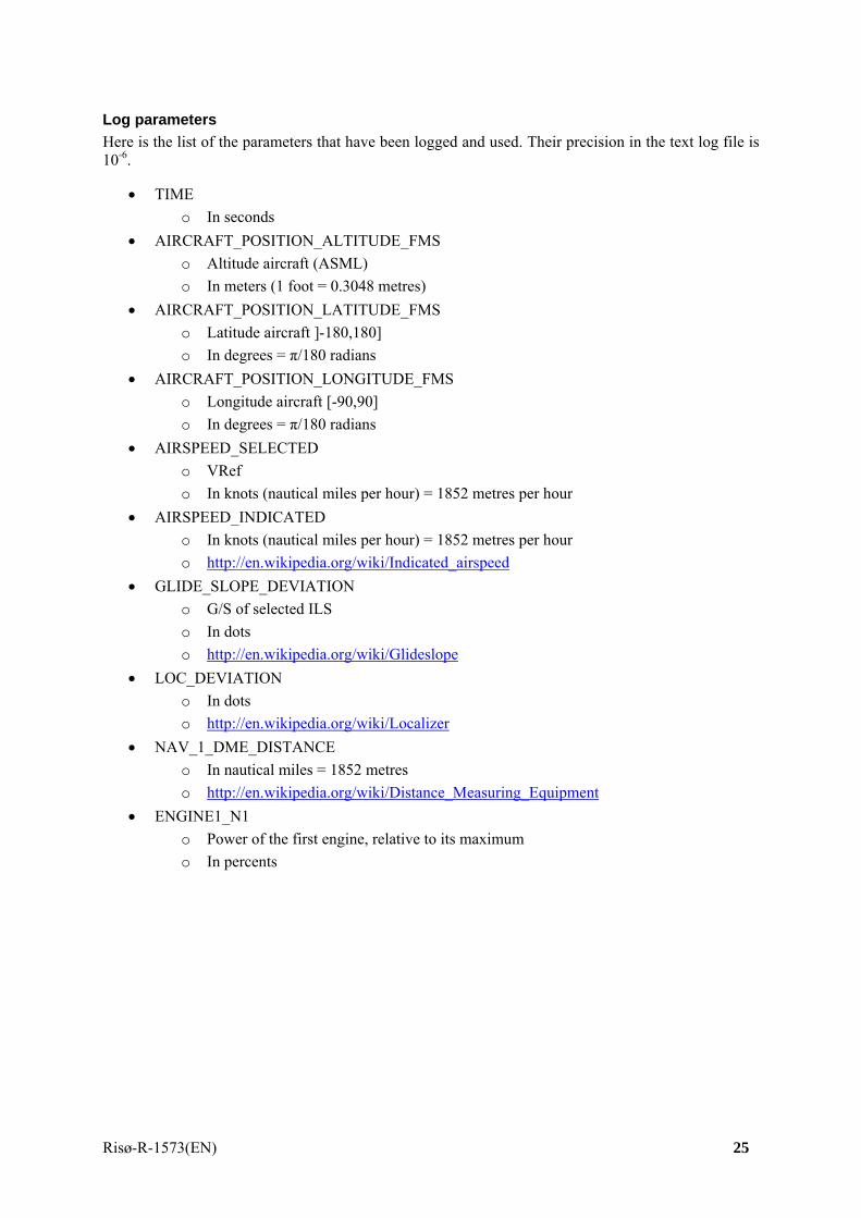
Log parameters Here is the list of the parameters that have been logged and used. Their precision in the text log file is 10-6.

• TIME o In seconds

• AIRCRAFT_POSITION_ALTITUDE_FMS o Altitude aircraft (ASML) o In meters (1 foot = 0.3048 metres)

• AIRCRAFT_POSITION_LATITUDE_FMS o Latitude aircraft ]-180,180] o In degrees = π/180 radians

• AIRCRAFT_POSITION_LONGITUDE_FMS o Longitude aircraft [-90,90] o In degrees = π/180 radians

• AIRSPEED_SELECTED o VRef o In knots (nautical miles per hour) = 1852 metres per hour

• AIRSPEED_INDICATED o In knots (nautical miles per hour) = 1852 metres per hour o http://en.wikipedia.org/wiki/Indicated_airspeed

• GLIDE_SLOPE_DEVIATION o G/S of selected ILS o In dots o http://en.wikipedia.org/wiki/Glideslope

• LOC_DEVIATION o In dots o http://en.wikipedia.org/wiki/Localizer

• NAV_1_DME_DISTANCE o In nautical miles = 1852 metres o http://en.wikipedia.org/wiki/Distance_Measuring_Equipment

• ENGINE1_N1 o Power of the first engine, relative to its maximum o In percents

Risø-R-1573(EN) 25

Approach and landing In the first set of experiments, the scenario was an approach and landing of an aircraft.

Approximations The geodesic 3D-model of the earth used in the following calculations is a spherical approximation with a radius of 6372795.0 meters.

Software A dedicated ad hoc program has been developed (named “Risø Geo distances”) in order to validate the geometric algorithms described below and their implementation. Known points have been used as input to check the correctness of the software. This program has also been used to make the numeric calculation of the following equations and distances.

Touch-down point coordinates The coordinates of the touch-down point, which is 300.0m after the beginning of the run-way, were given by Thales, by running a simulation where an aircraft has been moved to the touch-down point.

• Latitude: +43.621248° (north)

• Longitude: +1.369714° (east)

• Elevation: +154.589694m from sea level

Those coordinates were in agreement (± 12 meters) with some validation tests made with Google Earth [http://earth.google.com]. As a comparison, here are the coordinates of the touch-down point, visually positioned on Google Earth, with the “Measure” tool:

• Latitude: +43.621145° (north)

• Longitude: +1.369711° (east)

• Elevation: +151.0m from sea level

26 Risø-R-1573(EN)

See also Google Maps: [http://maps.google.com/maps?q=43.621145+1.369587&t=k]

Distance to touch-down It is not possible for an aircraft, which is in a 3D space, to land exactly on one point. Therefore, in order to ensure that the aircraft will intersect the touch-down reference, this reference will be a 3D-plane, orthogonal to the run-way, and including the touch-down point reference.

The longitudinal distance to touch down is the shortest linear distance from the centre of gravity of the plane to the reference touch-down 3D-plane described above.

The shape of the graphs using this way of measuring the distance to touch-down are showing very similar results with graphs using the DME distance.

A second point is needed for calculating the equation of the run-way. This second point, also given by Thales, is the start of the run-way, on the middle line:

Latitude: +43.619086° (north)

Longitude: +1.371992° (east)

Elevation: +154.589913m from sea level

Risø-R-1573(EN) 27

Touch-down 3D-plane equation Then, the equation of the touch-down 3D-plane (ax + by + cz + d = 0) has been calculated from one point and an orthogonal line. (See the algorithm of “Equation of a 3D-plane from one 3D-point and an orthogonal vector” for the details of the calculation)

• The touch-down point on the run-way: p

• The starting-point of the run-way: q

• The touch-down 3D-plane including the point p and orthogonal to the line (p, q)

o a = 161.463318673

o b = 187.345236307

o c = -174.088141238

o d = 44341.983539343

Centre line deviation The centre line of the run-way is modelled as a 3D-plane containing three points: the starting point of the run-way, the touch-down point, and the centre of the earth. In other words, this 3D-plane contains the run-way, and is vertical.

The lateral deviation is the shortest linear distance from the centre of gravity of the plane to the reference centre line 3D-plane described above.

28 Risø-R-1573(EN)

Centre line 3D-plane equation Equation of the touch-down 3D-plane (ax + by + cz + d = 0) from one point and an orthogonal line. (See the algorithm of “Equation of a 3D-plane from three 3D-points” for the details of the calculation)

• The touch-down point on the run-way: p

• The starting-point of the run-way: q

• The touch-down 3D-plane including the point p and orthogonal to the line (p, q)

o a = -842884492.548927000

o b = 1512815919.704380000

o c = 846260563.722481000

o d = 1.000000000

Risø-R-1573(EN) 29

Algorithms Here are detailed the algorithms used for the main calculations.

Conversion of a 3D-point to Cartesian In order to make the calculation, a 3D-point (longitude, latitude, elevation) is converted to a 3D-point (x, y, z) in a Cartesian geocentric grid, using a spherical geodesic approximation.

• Spherical geodesic approximation

o Radius (sea level): 6372795.0 meters from centre of the earth (mean radius)

//Conversion from degrees to radians latitude1 = latitude1 * PI / 180.0; longitude1 = longitude1 * PI / 180.0; //Conversion of the altitude from sea level, to centre of the earth seaLevel = 6372795.0; altitude1 = altitude1 + seaLevel; //Conversion to Cartesian radCosLat1 = altitude1 * Cos(latitude1); //Temporary variable x1 = radCosLat1 * Cos(longitude1); y1 = radCosLat1 * Sin(longitude1); z1 = altitude1 * Sin(latitude1);

Equation of a 3D-plane from one 3D-point and an orthogonal vector Plane containing a point p[x1, y1, z1], and orthogonal to the line (p, q) with q[x2, y2, z2].

Geometric vectors are used for the calculation.

Equation of the form ax + by + cz + d = 0;

//Vector (p, q) double[] v = new double[3]; v[0] = q[0] - p[0]; v[1] = q[1] - p[1]; v[2] = q[2] - p[2]; a = v[0]; b = v[1]; c = v[2]; d = - ((v[0] * p[0]) + (v[1] * p[1]) + (v[2] * p[2]));

30 Risø-R-1573(EN)

Equation of a 3D-plane from three 3D-points Plane containing three distinct points p[x1, y1, z1], q[x2, y2, z2] and r[x3, y3, z3]. Equation of the form ax + by + cz + d = 0; [Foley et al, Computer Graphics, 1995]. //Vector (p, q) v1[0] = q[0] - p[0]; v1[1] = q[1] - p[1]; v1[2] = q[2] - p[2]; //Vector (p, r) v2[0] = r[0] - p[0]; v2[1] = r[1] - p[1]; v2[2] = r[2] - p[2]; //v1 × v2 a = (v1[1] * v2[2]) - (v1[2] * v2[1]); b = (v1[2] * v2[0]) - (v1[0] * v2[2]); c = (v1[0] * v2[1]) - (v1[1] * v2[0]); //d d = - ((a * p[0]) + (b * p[1]) + (c * p[2]));

Distance between a 3D-point and a 3D-plane Shortest distance between a 3D-point s[x4, y4, z4] and a 3D-plane (ax + by + cz + d = 0).

distance = ((a * s[0]) + (b * s[1]) + (c * s[2]) + d) / Sqrt(Pow(a, 2) + Pow(b, 2) + Pow(c, 2));

Note that with this formula, with no absolute value for the numerator, one can obtain negative distances, which is an expected behaviour, since we want to know when the touch-down point has been passed, and if the plane is on the right or on the left of the centre line.

Graphs for approach and landing In order for our expert pilots to evaluate the relative quality of a landing compared with another one, the plotting of the path of the aircraft was needed, in a familiar format.

Three types of graphs have been produced, “Altitude”, “Centre line deviation”, “Speed deviation”, following a template given by the pilots. Two additional graphs have been made, “Glide path deviation” and “Localiser deviation”, in order to check the validity of the three first ones. They are indeed redundant with respectively “Altitude” and “Centre line deviation”.

The following examples are taken from the session 42 (09_13_05-14_35_21), with EVS on:

Risø-R-1573(EN) 31

32 Risø-R-1573(EN)

Risø-R-1573(EN) 33

Software Those graphs have been generated by a dedicated program using the algorithms above described. The output was at the SVG 1.1 standard format [http://www.w3.org/TR/SVG11/] (XML-based Scalable Vector Graphics), restricted to the “Tiny” profile [http://www.w3.org/TR/SVGMobile/]. SVG offered a convenient way to plot precisely what the pilots wanted, together with some zoom facilities.

The SVG graphs have then been viewed with the Opera 8.5 Web browser [http://www.opera.com] or Mozilla Firefox 1.5 Web browser [http://www.mozilla.com/firefox/].

34 Risø-R-1573(EN)

Validation For some of the lasts sessions, we have been able to get a plotting directly from the flight simulator. We have used them to validate our own figures.

Risø-R-1573(EN) 35

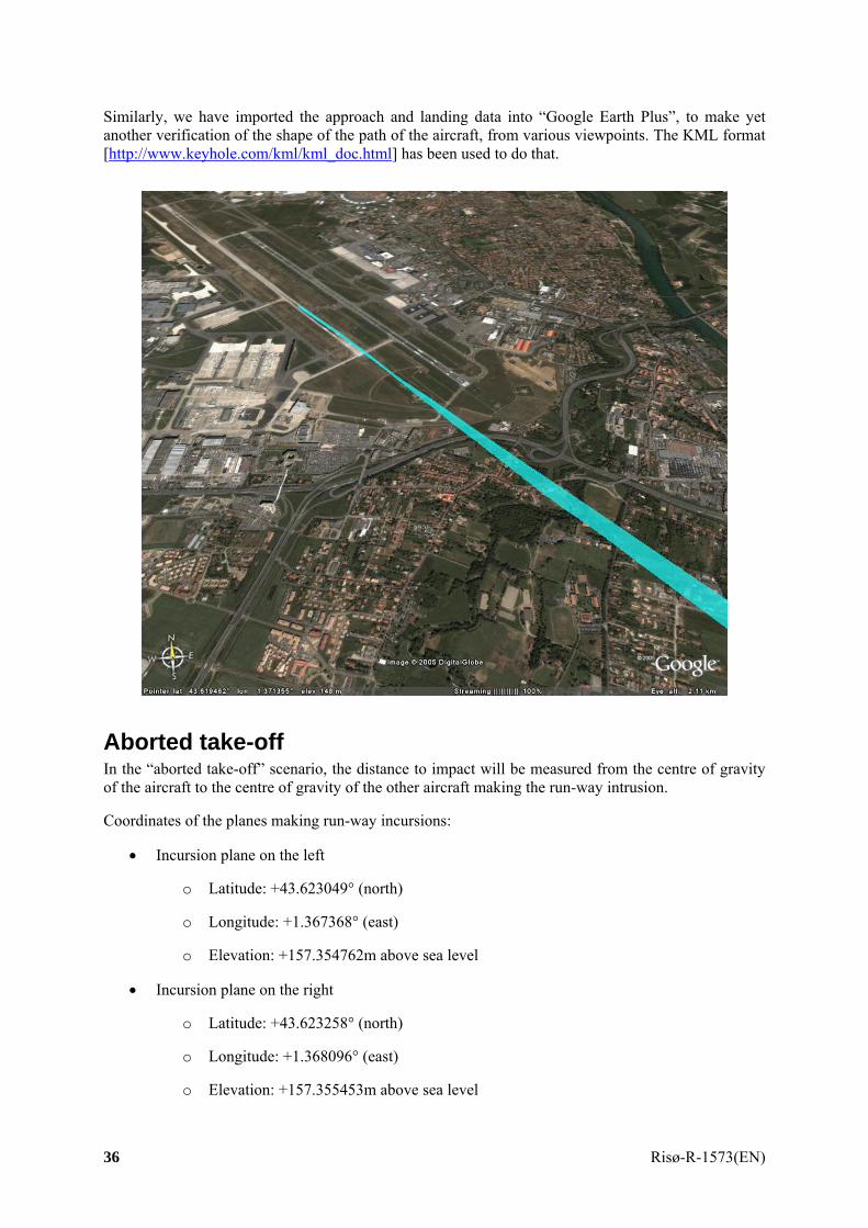
Similarly, we have imported the approach and landing data into “Google Earth Plus”, to make yet another verification of the shape of the path of the aircraft, from various viewpoints. The KML format [http://www.keyhole.com/kml/kml_doc.html] has been used to do that.

Aborted take-off In the “aborted take-off” scenario, the distance to impact will be measured from the centre of gravity of the aircraft to the centre of gravity of the other aircraft making the run-way intrusion.

Coordinates of the planes making run-way incursions:

• Incursion plane on the left

o Latitude: +43.623049° (north)

o Longitude: +1.367368° (east)

o Elevation: +157.354762m above sea level

• Incursion plane on the right

o Latitude: +43.623258° (north)

o Longitude: +1.368096° (east)

o Elevation: +157.355453m above sea level

36 Risø-R-1573(EN)

The incursion planes from the left and from the right are symmetric on the run-way axis. Therefore, the distances from the plane that is about to take-off to the incursion planes from the left or from the right are equal.

Measures For each session, the log files has been analysed to find when the obstacle has been detected by the pilot. This can be seen when the parameter ENGINE1_N1 is falling, indicating that the pilot has cut off the engines, and started to reverse them. This can also be seen when the speed of the aircraft starts to decrease.

The ENGINE1_N1 parameter was not available for the first crew (the first 4 sessions, out of 12). For the first 4 sessions, the AIRSPEED_INDICATED has been used, which is less accurate than ENGINE1_N1 (delayed by about 1 second), but sufficient to make relative comparisons between two sessions on this parameter.

The following example is taken from the session 29 (09_12_05-18_55_49), without EVS:

When the point of detection of the obstacle is known, the distance between the aircraft (longitude, latitude, altitude) and the obstacle (longitude, latitude, altitude) is then measured with the following algorithm.

Risø-R-1573(EN) 37

In this example from session 28 (09_12_05-18_53_55 with EVS), we can see that the pilot reacted 441.87 meters before the obstacle on the left.

The same type of calculation can be done when the aircraft starts, showing that the obstacle is 577.42 meters ahead, and when the speed falls down to zero, showing that the aircraft stopped 320.45 meters before the obstacle.

After the calculation of the absolute distance between two points, one must of course tell if the plane is before or after the obstacle. In addition to numeric calculation (similar to “approach and landing” distances), this can easily be seen on a 3D-map such as Google Earth.

Algorithms The algorithm “Conversion of a 3D-point to Cartesian” is the same as in the “approach and landing” scenario.

Distance between two Cartesian 3D-points Distance between two 3D-points p[x1, y1, z1] and q[x2, y2, z2].

distance = Sqrt(Pow(p[0] - q[0], 2) + Pow(p[1] - q[1], 2) + Pow(p[2] - q[2], 2));

Software As for the “approach and landing” scenario, the “Risø Geo distances” software has been used to measure the distance between the plane and the obstacle.

Remarks about the geometry calculation The author is aware that there are minor disagreements between the 3D-model used on the Thales simulator in Bordeaux, the 3D-map used on the simulator, the information given by the flight book for Blagnac flight data, the coordinates given by Google Earth, the geodesic sphere approximation of the algorithm used in this document, and reality. However, exact values are not that important for the purpose of the above SEE experiments, and the achieved precision should be more than enough to make relative comparisons. Finally, various checking, including data given by the DME distance, have proved to be consistent with distances obtained using calculation from longitude, latitude and elevation coordinates.

38 Risø-R-1573(EN)

Risø’s research is aimed at solving concrete problems in the society. Research targets are set through continuous dialogue with business, the political system and researchers. The effects of our research are sustainable energy supply and new technology for the health sector.

www.risoe.dk