SEEA Experimental Ecosystem Accounting:

Technical Recommendations

Final Draft

V3.2: 16 October 2017

Prepared as part of the joint UNEP / UNSD / CBD project on Advancing

Natural Capital Accounting funded by NORAD

ii

Preface

To be drafted by UNSD.

iii

Acknowledgements

The process of drafting these Technical Recommendations was undertaken under the auspices

of the United Nations Committee of Experts on Environmental-Economic Accounting

(UNCEEA). The Editorial Board on the SEEA Experimental Ecosystem Accounting (SEEA

EEA) and subsequently the Technical Committee on the SEEA EEA provided the technical

oversight of the drafting ensuring that comments received from difference sources were taken

into account during the drafting process. Many experts from countries as well as academia,

international, regional and nongovernmental-organizations from different disciplines such as

economics, ecosystem science, geoscience, policy and related fields participate in this exercise.

We would like to acknowledge the contributions to the Technical Recommendations of

individual experts and their organizations.

The Editorial Board members consisted of: Carl Obst (Editor), François Soulard (Statistics

Canada), Rocky Harris (Department for Environment, Food & Rural Affairs, UK), Anton

Steurer (Eurostat), Jan-Erik Petersen (European Environment Agency), Michael Bordt (UN

ESCAP), Daniel Juhn (Conservation International), Lars Hein (Wageningen University, the

Netherlands), Alessandra Alfieri and Julian Chow (United Nations Statistics Division) and the

World Bank.

Members of the UNCEEA and other contributors from national institutions: Lisa Wardlaw-

Kelly, John Power, Matt Jakab, Steve May (Australia), Sacha Baud (Austria), Norbu Ugyen,

Sonam Laendup, Lobzang Dorji (Bhutan), Wadih Joao Scandar Neto, Luana Magalhaes Duarte

(Brazil), Andre Loranger, Carolyn Cahill, François Soulard, Mark Henry, Gabriel Gagnon,

Jennie Wang, Stéphanie Uhde, Kevin Roberts (Canada), Claudia Cortés, Jorge Gómez, Rafael

Marcial Agacino Rojas (Chile), Qiong Qiu, Qin Tian, Shi Faqi (China), Gloria Lucia Vargas

Briceno (Colombia), Kirsten Wismer (Denmark), Jukka Muukkonen, Petteri Vihervaara

(Finland), Francoise Nirascou (France), Sven Christian Kaumanns, Beyhan Ekinci (Germany),

Rakesh Kumar Maurya, Davendra Verma, James Mathew (India), Etjih Tasriah, Buyung

Airlangga (Indonesia), Aldo Maria Femia, Angelica Tudini (Italy), Stephane Henriod

(Kyrgyzstan), Nazaria Baharudin, Zarinah Mahari (Malaysia), Nourudeen Jaffar (Mauritius),

José Arturo Blancas Espejo, Raúl Figueroa Díaz, Francisco Javier Jiménez Nava, Melanie Kolb

(Mexico), Ankhzaya Byamba, Erdenesan Eldevochir (Mongolia), Bert Kroese, Sjoerd Schenau,

Rixt de Jong, Stefan van der Esch, Clara Veerkamp, Arjan Ruijs, Petra van Egmond, Gerard

Eding (Netherlands), David N. Barton, Per Arild Garnåsjordet, Iulie Aslaksen, Kristine

Grimsrud (Norway), Vivian Ilarina, Romeo Recide (Philippines), Andrey Tatarinov (Russia),

Aliielua Salani (Samoa), Johannes de Beer, Robert Parry, Amanda Driver, Ester Koch (South

Africa), Nancy Steinbach and Viveka Palm (Sweden), Samuel Echoku (Uganda), Gemma

Thomas, Rocky Harris, James Evans (United Kingdom), Dennis Fixler, Dixon Landers, Charles

Rhodes, Dylan Rassier, Robert McKane, Roger Sayre (USA), Duong Manh Hung, Pham Tien

Nam, Kim Thi Thu, Hoang Lien Son (Viet Nam).

Representatives from international organizations: Jan-Erik Petersen, Daniel Desaulty, Nihat

Zal and Lisa Waselikowski, Caitriona Maguire (European Environment Agency), Anton

Steurer, Veronika Vysna (Eurostat), Jakub Wejchert and Laure Ledoux (European

Commission, DG Environment), Alessandra La Notte, Joachim Maes (European Commission,

Joint Research Center), Jesús Alquézar (European Commission, DG Research and Innovation),

iv

Francesco Tubiello, Silvia Cerilli (FAO), Kimberly Dale Zieschang (International Monetary

Fund), Myriam Linster, Peter van de Ven (OECD), Arnaud Comolet, Jean-Louis Weber

(Convention on Biological Diversity), Barbro Elise Hexeberg, Glenn-Marie Lange, Ken

Bagstad, Michael Vardon, Juan-Pueblo Castaneda, Sofia Ahlroth, Grant Cameron (World

Bank), Alexander Dominik Erlewein (UNCCD), Tim Scott and Massimiliano Riva (UNDP),

Emmanuel Ngok (UNECA), Michael Nagy (UNECE), Rayen Quiroga (UNECLAC), Michael

Bordt (UNESCAP), Jillian Campbell, Pushpam Kumar (UNEP), Steven King, Claire Brown,

Lucy Wilson (UNEP-WCMC), William Reidhead (UN-Water), Clara van der Pol (UNWTO).

Other experts that provided expert opinion: David Vačkář (Academy of Sciences of the Czech

Republic), Michael Vardon, Heather Keith (Australian National University), Ferdinando Villa

(Basque Centre for Climate Change), Roel Boumans (Boston University), Mahbubul Alam,

Hedley Grantham, Miro Honsak, Daniel Juhn, Rosimeiry Portela, Ana Maria Rodriguez,

Mahbubul Alam, Timothy Wright, Trond Larsen (Conservation International), David A.

Robinson, Bridget Emmett (Centre for Ecology and Hydrology, UK), Jeanne Nel (Council for

Scientific and Industrial research, South Africa), Leo Denocker, Steven Broekx, Inge Liekens,

Sander Jacobs (INBO research group Nature and Society, via BEES international working

group), Nathalie Olsen (International Union for conservation of Nature), Louise Gallagher (Luc

Hoffmann Institute at World Wildlife Fund International), Wilbert Van Rooij (Plansup), Guy

Ziv (University of Leeds), Emil Ivanov (University of Nottingham), Louise Willemen

(University of Twente, Netherlands), Mariyana Lyubenova (University of Sofia, Bulgaria),

Bethanna Jackson (Victoria University of Wellington), Lars Hein (Wageningen University,

Netherlands).

United Nations Statistics Division staff and consultants: Alessandra Alfieri, Jessica Chan,

Julian Chow, Ivo Havinga, Bram Edens (formerly with Statistics Netherlands), Mark

Eigenraam, Emil Ivanov, Marko Javorsek, Leila Rohd-Thomsen, Sokol Vako.

The drafting of the Technical Recommendations was supported by the United Nations Statistics

Division, the United Nations Environment, the Secretariat of the Convention on Biological

Diversity and the Norwegian Agency Cooperation through the Advancing Natural Capital

Accounting (ANCA) project. The project aimed to support countries in efforts to embark on

the SEEA Experimental Ecosystem Accounting with a view to improving the management of

ecosystem services.

Financial contributors to the drafting of the Technical Recommendations were provided by the

Norwegian Agency for Development Cooperation through the ANCA project and the European

Union.

v

Contents

Preface ii

Acknowledgements ................................................................................................................. iii

Contents v

List of tables ............................................................................................................................. x

List of figures ........................................................................................................................... x

List of abbreviations and acronyms ......................................................................................... xi

1 Introduction ...................................................................................................................... 1

1.1 Definition of ecosystem accounting ......................................................................... 1

1.1.1 The conceptual motivation .................................................................................. 1

1.1.2 The central measurement objective of ecosystem accounting ............................. 3

1.1.3 Measurement pathways ....................................................................................... 6

1.1.4 Uses and applications of ecosystem accounting .................................................. 8

1.2 Scope and purpose of the SEEA EEA Technical Recommendations .................... 10

1.2.1 Connection to the SEEA EEA ........................................................................... 10

1.2.2 Connection to the SEEA Central Framework .................................................... 10

1.2.3 Connection to other ecosystem accounting and similar materials ..................... 11

1.2.4 The audience for the Technical Recommendations ........................................... 11

1.2.5 Implementation of ecosystem accounting .......................................................... 12

1.3 Developments to SEEA EEA incorporated into the Technical Recommendations 14

1.3.1 Introduction ....................................................................................................... 14

1.3.2 The treatment of spatial units ............................................................................ 14

1.3.3 Account labelling and structure ......................................................................... 14

1.3.4 The measurement of ecosystem services ........................................................... 15

1.3.5 Ecosystem condition .......................................................................................... 16

1.3.6 Ecosystem capacity ............................................................................................ 16

1.4 Structure of Technical Recommendations ............................................................. 16

2 Ecosystem accounts and approaches to measurement .................................................... 18

2.1 Introduction ............................................................................................................ 18

2.2 The SEEA EEA ecosystem accounting framework ............................................... 18

2.3 The ecosystem accounts ......................................................................................... 21

2.3.1 Placing the ecosystem accounts in context ........................................................ 21

2.3.2 Ecosystem extent accounts ................................................................................ 22

2.3.3 Ecosystem condition accounts ........................................................................... 23

2.3.4 Ecosystem services supply and use accounts .................................................... 23

vi

2.3.5 Ecosystem monetary asset account .................................................................... 24

2.3.6 Related accounts and concepts .......................................................................... 24

2.4 The steps in compiling ecosystem accounts ........................................................... 26

2.4.1 Introduction ....................................................................................................... 26

2.4.2 Summary of compilation steps for developing the full set of accounts ............. 28

2.5 Key considerations in compiling ecosystem accounts ........................................... 30

3 Organising spatial data and accounting for ecosystem extent ........................................ 34

3.1 Introduction ............................................................................................................ 34

3.2 The framework for delineating spatial areas for ecosystem accounting ................ 35

3.2.1 Introduction ....................................................................................................... 35

3.2.2 Ecosystem Assets (EA)...................................................................................... 37

3.2.3 Ecosystem Type (ET) ........................................................................................ 38

3.2.4 Ecosystem Accounting Area (EAA) .................................................................. 40

3.3 The ecosystem extent account ................................................................................ 41

3.4 Compiling the ecosystem extent account ............................................................... 42

3.5 Spatial infrastructure, measurement, and data layers ............................................. 43

3.5.1 Basic spatial units (BSU) ................................................................................... 43

3.5.2 Data layers and delineation ................................................................................ 45

3.6 Recommendations for developing a National Spatial Data Infrastructure (NSDI) and

the compilation of ecosystem extent accounts .................................................................... 47

3.6.1 Developing an NSDI.......................................................................................... 47

3.6.2 Recommendations for developing the ecosystem extent account ...................... 48

3.7 Key research issues in delineating spatial areas for ecosystem accounting ........... 51

4 The ecosystem condition account ................................................................................... 53

4.1 Introduction ............................................................................................................ 53

4.2 Different approaches to the measurement of ecosystem condition ........................ 55

4.3 Ecosystem condition accounts ............................................................................... 56

4.4 Developing indicators of individual ecosystem characteristics ............................. 58

4.4.1 Selecting indicators ............................................................................................ 58

4.4.2 Aggregate measures of condition ...................................................................... 61

4.4.3 Determining a reference condition .................................................................... 63

4.5 Recommendations for compiling ecosystem condition accounts .......................... 65

4.6 Issues for research on ecosystem condition ........................................................... 67

5 Accounting for flows of ecosystem services .................................................................. 68

5.1 Introduction ............................................................................................................ 68

5.2 Ecosystem services supply and use accounts ......................................................... 69

5.2.1 Introduction ....................................................................................................... 69

5.2.2 Overall structure of the supply and use accounts .............................................. 70

vii

5.2.3 Connections to the SEEA Central Framework .................................................. 71

5.2.4 Recording the connection to economic units ..................................................... 72

5.2.5 Compiling the ecosystem services supply table ................................................ 73

5.2.6 Compiling the ecosystem services use table ...................................................... 74

5.3 Issues in the definition of ecosystem services ........................................................ 75

5.3.1 Introduction ....................................................................................................... 75

5.3.2 Distinguishing ecosystem services and benefits ................................................ 76

5.3.3 Distinguishing final and intermediate ecosystem services ................................ 77

5.3.4 The treatment of other environmental goods and services ................................ 79

5.3.5 The link between biodiversity and ecosystem services ..................................... 79

5.3.6 The treatment of ecosystem disservices............................................................. 80

5.3.7 The scope of cultural services within an accounting framework ....................... 81

5.4 The classification of ecosystem services................................................................ 81

5.4.1 Introduction ....................................................................................................... 81

5.4.2 Proposed approach to the use of classifications ................................................. 82

5.5 The role and use of biophysical modelling ............................................................ 87

5.5.1 Introduction ....................................................................................................... 87

5.5.2 Overview of biophysical modelling approaches ................................................ 87

5.6 Data sources, materials and methods for measuring ecosystem service flows ...... 89

5.6.1 Introduction ....................................................................................................... 89

5.6.2 Data sources ....................................................................................................... 89

5.6.3 Measuring the supply of ecosystem services ..................................................... 91

5.6.4 Recording the users of ecosystem services ........................................................ 92

5.7 Recommendations for the measurement of ecosystem services ............................ 93

5.8 Key areas for research ............................................................................................ 95

6 Valuation in ecosystem accounting ................................................................................ 97

6.1 Introduction ............................................................................................................ 97

6.2 Valuation principles for ecosystem accounting ..................................................... 98

6.2.1 Introduction ....................................................................................................... 98

6.2.2 Establishing the markets for exchange values ................................................... 99

6.2.3 Estimation of changes in welfare and consumer surplus ................................. 100

6.3 Relevant data and source materials ...................................................................... 102

6.3.1 Introduction ..................................................................................................... 102

6.3.2 Potential valuation techniques ......................................................................... 103

6.3.3 Alternatives to direct monetary valuation ........................................................ 107

6.4 Key challenges and areas for research in valuation ............................................. 107

6.5 Recommendations on the valuation of ecosystem services ................................. 111

viii

7 Accounting for the value and capacity of ecosystem assets ......................................... 113

7.1 Introduction .......................................................................................................... 113

7.2 Ecosystem monetary asset account ...................................................................... 114

7.2.1 Description of the account ............................................................................... 114

7.2.2 Measurement of net present value ................................................................... 117

7.3 Measuring ecosystem capacity ............................................................................. 120

7.3.1 Defining ecosystem capacity ........................................................................... 120

7.3.2 Linking ecosystem capacity and ecosystem degradation................................. 122

7.4 Recording ecosystem degradation........................................................................ 124

7.4.1 Accounting entries for degradation and depletion ........................................... 124

7.4.2 Allocation of ecosystem degradation to economic units ................................. 125

7.4.3 On the use of the restoration cost approach to value ecosystem degradation .. 125

7.5 Recommendations for compiling ecosystem monetary asset accounts ................ 126

7.6 Key issues for research ........................................................................................ 127

8 Integrating ecosystem accounting information with standard national accounts ......... 128

8.1 Introduction .......................................................................................................... 128

8.2 Steps required for full integration with the national accounts ............................. 129

8.3 Combined presentations ....................................................................................... 130

8.4 Extended supply and use accounts ....................................................................... 131

8.5 Integrated sequence of institutional sector accounts ............................................ 133

8.6 Extended and integrated balance sheets ............................................................... 136

8.7 Alternative approaches to integration .................................................................. 138

8.8 Recommendations ................................................................................................ 139

9 Thematic accounts ........................................................................................................ 141

9.1 Introduction .......................................................................................................... 141

9.2 Accounting for land ............................................................................................. 142

9.2.1 Introduction ..................................................................................................... 142

9.2.2 Relevant data and source materials .................................................................. 144

9.2.3 Key issues and challenges in measurement ..................................................... 144

9.2.4 Recommended activities and research issues .................................................. 145

9.3 Accounting for water related stocks and flows .................................................... 146

9.3.1 Introduction ..................................................................................................... 146

9.3.2 Relevant data and source materials .................................................................. 147

9.3.3 Key issues and challenges in measurement ..................................................... 147

9.3.4 Recommended activities and research issues .................................................. 148

9.4 Accounting for carbon related stocks and flows .................................................. 148

9.4.1 Introduction ..................................................................................................... 148

ix

9.4.2 Relevant data and source materials .................................................................. 149

9.4.3 Key issues and challenges in measurement ..................................................... 149

9.4.4 Recommended activities and research issues .................................................. 149

9.5 Accounting for biodiversity ................................................................................. 150

9.5.1 Introduction ..................................................................................................... 150

9.5.2 Assessing ecosystem-level and species-level biodiversity .............................. 151

9.5.3 Implementing biodiversity accounting ............................................................ 153

9.5.4 Limitations and issues to resolve ..................................................................... 154

9.5.5 Recommendations for testing and further research ......................................... 154

9.6 Other thematic accounts and data on drivers of ecosystem change ..................... 155

Annex 1: Summary of various Natural Capital Accounting initiatives ................................ 157

International and national initiatives ................................................................................. 157

Corporate initiatives .......................................................................................................... 162

Annex 2: Key features of a national accounting approach to ecosystem measurement ....... 164

Introduction ....................................................................................................................... 164

Key features of a national accounting approach ................................................................ 165

Applying the national accounting approach to ecosystem accounting .............................. 166

Principles and tools of national accounting ....................................................................... 167

References 171

x

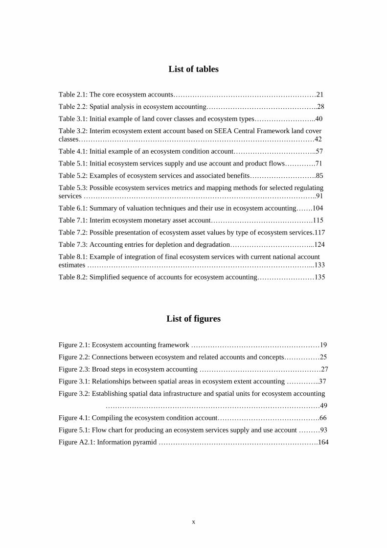
List of tables

Table 2.1: The core ecosystem accounts……………………………………………………21

Table 2.2: Spatial analysis in ecosystem accounting………………………………………..28

Table 3.1: Initial example of land cover classes and ecosystem types……………………..40

Table 3.2: Interim ecosystem extent account based on SEEA Central Framework land cover

classes………………………………………………………………………………………42

Table 4.1: Initial example of an ecosystem condition account……………………………..57

Table 5.1: Initial ecosystem services supply and use account and product flows………….71

Table 5.2: Examples of ecosystem services and associated benefits……………………….85

Table 5.3: Possible ecosystem services metrics and mapping methods for selected regulating

services ……………………………………………………………………………………..91

Table 6.1: Summary of valuation techniques and their use in ecosystem accounting…….104

Table 7.1: Interim ecosystem monetary asset account…………………………………….115

Table 7.2: Possible presentation of ecosystem asset values by type of ecosystem services.117

Table 7.3: Accounting entries for depletion and degradation……………………………...124

Table 8.1: Example of integration of final ecosystem services with current national account

estimates …………………………………………………………………………………...133

Table 8.2: Simplified sequence of accounts for ecosystem accounting……………………135

List of figures

Figure 2.1: Ecosystem accounting framework ………………………………………………19

Figure 2.2: Connections between ecosystem and related accounts and concepts……………25

Figure 2.3: Broad steps in ecosystem accounting ……………………………………………27

Figure 3.1: Relationships between spatial areas in ecosystem extent accounting …………..37

Figure 3.2: Establishing spatial data infrastructure and spatial units for ecosystem accounting

………………………………………………………………………………49

Figure 4.1: Compiling the ecosystem condition account…………………………………….66

Figure 5.1: Flow chart for producing an ecosystem services supply and use account ………93

Figure A2.1: Information pyramid ………………………………………………………….164

xi

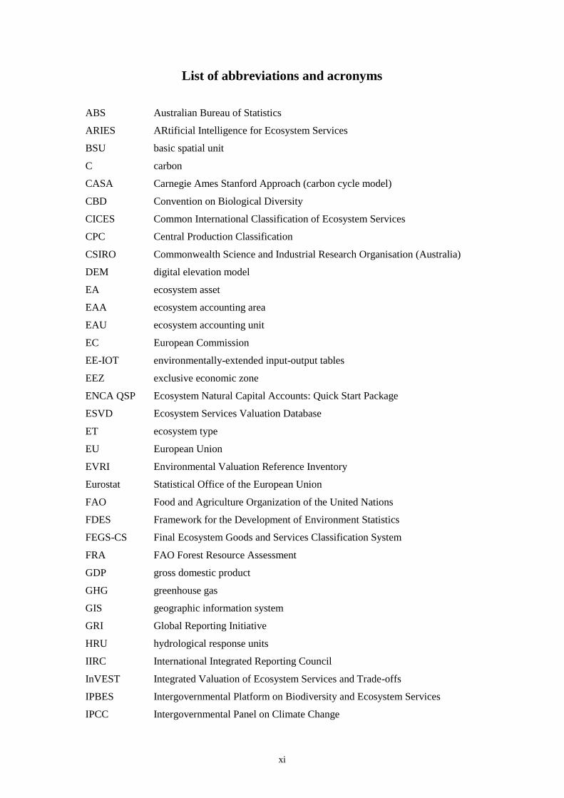
List of abbreviations and acronyms

ABS Australian Bureau of Statistics

ARIES ARtificial Intelligence for Ecosystem Services

BSU basic spatial unit

C carbon

CASA Carnegie Ames Stanford Approach (carbon cycle model)

CBD Convention on Biological Diversity

CICES Common International Classification of Ecosystem Services

CPC Central Production Classification

CSIRO Commonwealth Science and Industrial Research Organisation (Australia)

DEM digital elevation model

EA ecosystem asset

EAA ecosystem accounting area

EAU ecosystem accounting unit

EC European Commission

EE-IOT environmentally-extended input-output tables

EEZ exclusive economic zone

ENCA QSP Ecosystem Natural Capital Accounts: Quick Start Package

ESVD Ecosystem Services Valuation Database

ET ecosystem type

EU European Union

EVRI Environmental Valuation Reference Inventory

Eurostat Statistical Office of the European Union

FAO Food and Agriculture Organization of the United Nations

FDES Framework for the Development of Environment Statistics

FEGS-CS Final Ecosystem Goods and Services Classification System

FRA FAO Forest Resource Assessment

GDP gross domestic product

GHG greenhouse gas

GIS geographic information system

GRI Global Reporting Initiative

HRU hydrological response units

IIRC International Integrated Reporting Council

InVEST Integrated Valuation of Ecosystem Services and Trade-offs

IPBES Intergovernmental Platform on Biodiversity and Ecosystem Services

IPCC Intergovernmental Panel on Climate Change

xii

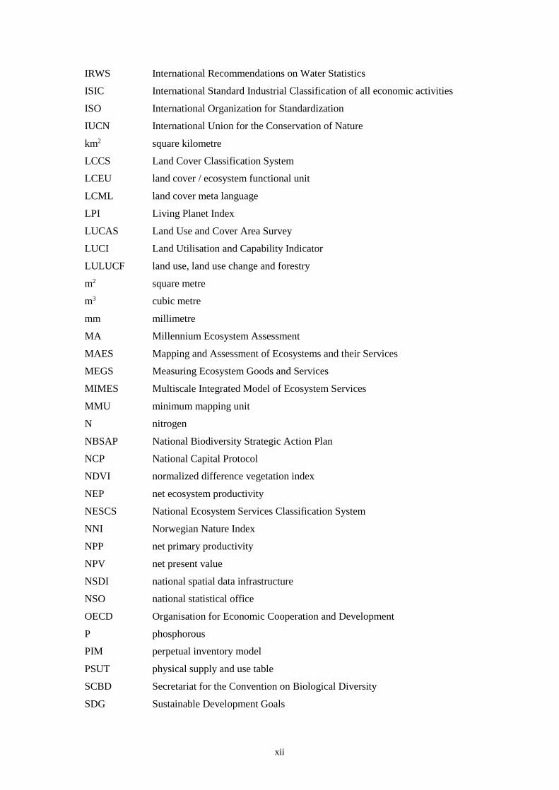
IRWS International Recommendations on Water Statistics

ISIC International Standard Industrial Classification of all economic activities

ISO International Organization for Standardization

IUCN International Union for the Conservation of Nature

km2 square kilometre

LCCS Land Cover Classification System

LCEU land cover / ecosystem functional unit

LCML land cover meta language

LPI Living Planet Index

LUCAS Land Use and Cover Area Survey

LUCI Land Utilisation and Capability Indicator

LULUCF land use, land use change and forestry

m2 square metre

m3 cubic metre

mm millimetre

MA Millennium Ecosystem Assessment

MAES Mapping and Assessment of Ecosystems and their Services

MEGS Measuring Ecosystem Goods and Services

MIMES Multiscale Integrated Model of Ecosystem Services

MMU minimum mapping unit

N nitrogen

NBSAP National Biodiversity Strategic Action Plan

NCP National Capital Protocol

NDVI normalized difference vegetation index

NEP net ecosystem productivity

NESCS National Ecosystem Services Classification System

NNI Norwegian Nature Index

NPP net primary productivity

NPV net present value

NSDI national spatial data infrastructure

NSO national statistical office

OECD Organisation for Economic Cooperation and Development

P phosphorous

PIM perpetual inventory model

PSUT physical supply and use table

SCBD Secretariat for the Convention on Biological Diversity

SDG Sustainable Development Goals

xiii

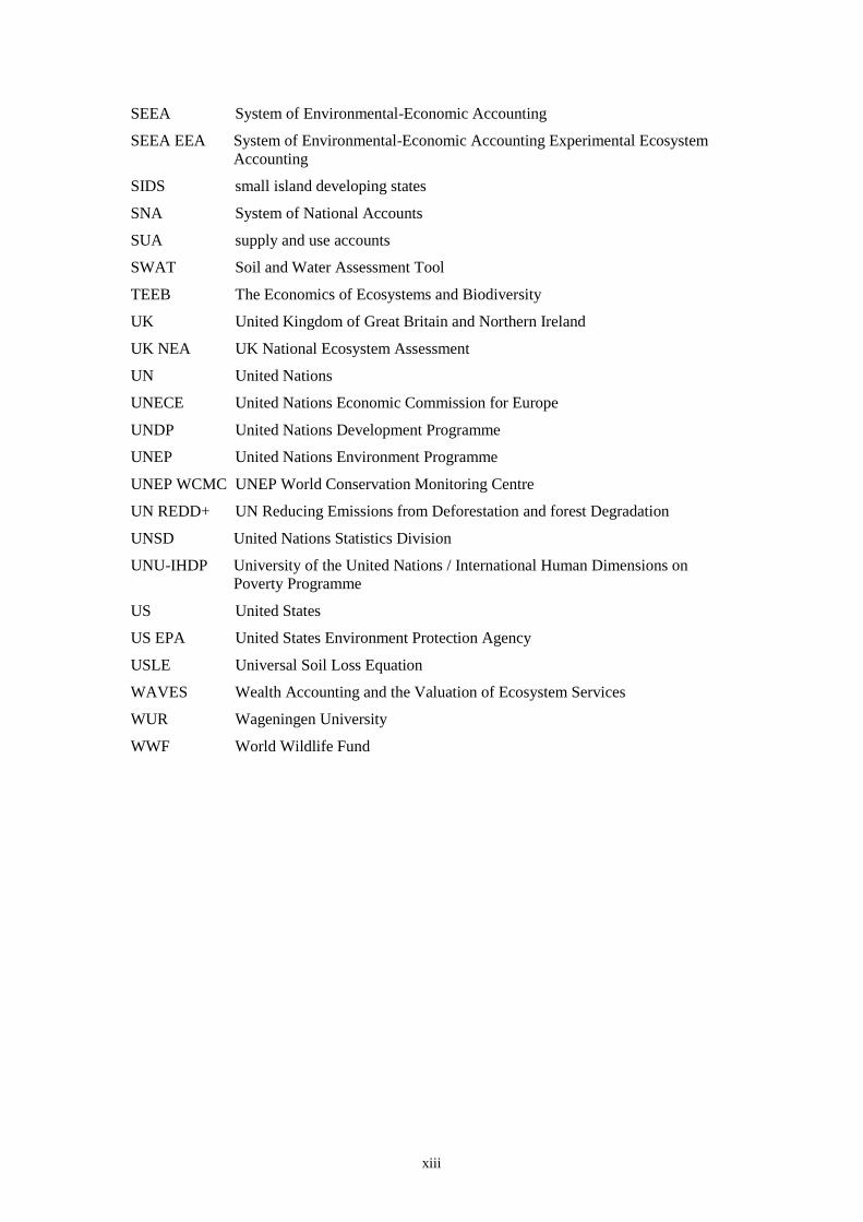
SEEA System of Environmental-Economic Accounting

SEEA EEA System of Environmental-Economic Accounting Experimental Ecosystem

Accounting

SIDS small island developing states

SNA System of National Accounts

SUA supply and use accounts

SWAT Soil and Water Assessment Tool

TEEB The Economics of Ecosystems and Biodiversity

UK United Kingdom of Great Britain and Northern Ireland

UK NEA UK National Ecosystem Assessment

UN United Nations

UNECE United Nations Economic Commission for Europe

UNDP United Nations Development Programme

UNEP United Nations Environment Programme

UNEP WCMC UNEP World Conservation Monitoring Centre

UN REDD+ UN Reducing Emissions from Deforestation and forest Degradation

UNSD United Nations Statistics Division

UNU-IHDP University of the United Nations / International Human Dimensions on

Poverty Programme

US United States

US EPA United States Environment Protection Agency

USLE Universal Soil Loss Equation

WAVES Wealth Accounting and the Valuation of Ecosystem Services

WUR Wageningen University

WWF World Wildlife Fund

1

1 Introduction

1.1 Definition of ecosystem accounting

1.1.1 The conceptual motivation

1.1 Ecosystem accounting is a coherent framework for integrating measures of

ecosystems and the flows of services from them with measures of economic and other

human activity. Ecosystem accounting complements, and builds on, the accounting for

environmental assets as described in the System of Environmental-Economic

Accounting (SEEA) Central Framework (UN, et al., 2014a). In the SEEA Central

Framework, environmental assets are accounted for as individual resources such as

timber resources, soil resources and water resources. In ecosystem accounting as

described in the SEEA Experimental Ecosystem Accounting (SEEA EEA) (UN et al.,

2014b), the accounting approach recognises that these individual resources function in

combination within a broader system.

1.2 The prime motivation for ecosystem accounting is that separate analysis of

ecosystems and the economy does not adequately reflect the fundamental relationship

between humans and the environment. In this context, the SEEA EEA accounting

framework provides a common platform for the integration of (i) information on

ecosystem assets (i.e. ecosystem extent, ecosystem condition, ecosystem services and

ecosystem capacity), and (ii) existing accounting information on economic and other

human activity dependent upon ecosystems and the associated beneficiaries

(households, businesses and governments).

1.3 The integration of ecosystem and economic information is intended to

mainstream information on ecosystems within decision making. Consequently, there

must be a strong relevance of the information set to current issues of concern. The

intent of ecosystem accounting described in the SEEA EEA was for application of the

framework at a national level. That is, linking information on multiple ecosystem types

and multiple ecosystem services with macro level economic information such as

measures of national income, production, consumption and wealth.

1.4 However, since the first release of the SEEA EEA it has proved relevant to

apply the SEEA EEA ecosystem accounting framework at regional and sub-national

scales. For example, for individual administrative areas such as provinces, protected

areas and cities; and environmentally defined areas such as water catchments. Indeed,

at these sub-national scales, the potential of ecosystem accounting can be demonstrated

more easily by linking directly to the development of responses to specific policy

themes or issues. Thus, a sub-national focus may be of particular interest in the

development of pilot studies on ecosystem accounting and one that is facilitated by the

increasing availability of data about ecosystems at this detailed level.

1.5 Importantly, using a common accounting framework for the measurement and

organisation of data at sub-national levels, supports the development of a more

complete national picture. This same logic also extends to the co-ordination of

ecological information on trans-boundary and global scales. Overall, the co-ordination

and integration of data using an accounting framework can provide a rich information

base for both local and broad scale ecosystem and natural resource management.

1.6 The essence of ecosystem accounting is that the biophysical environment can

be partitioned to form a set of ecosystem assets. Potential ecosystem assets include

forests, wetlands, agricultural areas, rivers and coral reefs. Focus to date has been on

accounting for land areas, including inland waters, but there are also applications for

2

coastal and marine areas. 1 Each ecosystem asset is then accounted for in a manner

analogous to the treatment of produced assets such as buildings and machines in the

System of National Accounts (SNA) (EC, et al., 2009).2 The analogous treatment

implies that ecological information pertaining to ecosystems can be recorded using the

same measurement framework that is used to record information on produced and other

economic assets. Thus, the stock and change in stock of each asset is recorded as a

combination of (i) balance sheet entries at points in time and (ii) changes in assets such

as via investment or depreciation and degradation.

1.7 Each ecosystem asset supplies a stream of ecosystem services. For produced

assets, the services provided are known as capital services (e.g. housing services

provided by a dwelling). The flows of services (both for ecosystem assets and produced

assets) in any period are related to the productive capacity of the asset. These services

also generate an income flow for the economic unit that owns or manages the asset and

they are inputs to the production of other goods and services. This fundamental

accounting model remains consistent throughout these recommendations. Box 1.1

provides additional introductory material on defining stocks and flows in an accounting

context.

Box 1.1 Recording stocks and flows for accounting

The terms stocks and flows are commonly used in measurement discussions but can be applied in

different ways from those intended from an accounting perspective. For accounting purposes, the

stocks refer to the underlying assets that support production and the generation of income. Stocks

are measured at the beginning and end of each accounting period (e.g. the end of the financial year)

and these measurements are aggregated to form a balance sheet for that point in time. Information

about stocks may be recorded in physical terms (e.g. the hectares of plantation forest) and in

monetary terms.

For ecosystem accounting, the stocks of primary focus are the ecosystem assets delineated within

the area in scope of the accounts. Conceptually, information about each ecosystem asset, for example

information on its extent, condition and monetary value, can be recorded at the beginning and end

of each accounting period and thus contribute to understanding the potential for the stock to support

the generation of ecosystem services into the future (ecosystem capacity).

Two types of flows are recorded in accounting, namely (i) changes in stock and (ii) flows related to

production, consumption and income. Changes in stock include additions to stock as a result of

investment or, in the case of ecosystem assets, natural growth and improvements in condition; and

reductions in stock due to extraction, degradation or natural loss.

Concepts of production, consumption and income are all flow concepts. For ecosystem accounting,

the relevant flows relate to the supply and use of ecosystem services between ecosystem assets and

beneficiaries including businesses, governments and households. Benefits as described in ecosystem

accounting are also flows.

It is important to be clear about the distinction between these two types of flows since they should

not be aggregated. A common incorrect treatment is to consider improvements in the condition of

ecosystem assets to be flows that can be combined with flows of ecosystem services. Instead, the

appropriate treatment is to consider that improvements in condition increase the capacity of the

ecosystem asset to generate ecosystem services. Thus, the different types of flows have distinct

interpretations in accounting.

The distinction between stocks and the two types of flows as described here supports conveying a

story about the relationship between the maintenance and degradation of ecosystem assets on the

one hand, and the supply of ecosystem services on the other. By gathering information on both

aspects, the accounting framework supports analysis of ecosystem capacity and sustainability in a

manner aligned with standard economic and financial analysis.

1 For applications for marine areas (see section 3.7). 2 As developed in economics by Solow, Jorgenson and others in the 1950s and 1960s and applied actively

in national accounting from the 1990s (OECD, 2009). The SNA is the international statistical standard for

the compilation of national economic accounts.

3

1.8 The accounting framework described in SEEA EEA extends, supports and

complements other ecosystem and biodiversity measurement initiatives in four

important ways.

• First, the SEEA EEA framework involves accounting for ecosystem assets in terms

of both ecosystem condition and ecosystem services. Often, measurement of

condition and ecosystem services is undertaken in separate fields of research, and

there are relatively few studies that conceptualise ecosystem assets and services in

the comprehensive manner described here.3

• Second, the SEEA EEA framework encompasses accounting in both biophysical

terms (e.g. hectares, tonnes) and in monetary terms using various valuation

techniques.

• Third, the SEEA EEA framework is designed to facilitate comparison and

integration with the economic data prepared following the System of National

Accounts (SNA). This leads to the adoption of certain measurement boundaries

and valuation concepts that are not systematically applied in other forms of

ecosystem measurement. The use of SNA derived measurement principles and

concepts facilitates the mainstreaming of ecosystem information with standard

measures of income, production and wealth.

• Fourth, the general intent of the SEEA EEA framework is to provide a broad, cross-

cutting perspective on ecosystems at a country or large, sub-national level.

However, many ecosystem measurements are conducted at a detailed, local level.

The SEEA EEA framework provides an organizing structure by which detailed

data can be placed in context and used to paint a rich picture of the condition of

ecosystems and the services they supply.

1.1.2 The central measurement objective of ecosystem accounting

1.9 The SEEA EEA has emerged from work initiated by the international

community of official statisticians, particularly the national accounts community, and

their development of the SEEA Central Framework. There has long been recognition

of ecosystems in the context of environmental-economic accounting, and recognition

of the need to account for the degradation of ecosystems. However, the national

accounting based approach described in the SEEA EEA has only emerged in recent

years, as official statisticians have worked to synthesise the substantial literature

concerning ecosystems and ecosystem services.

1.10 This conceptual framing is elaborated at greater length through the remaining

chapters. However, at an introductory level, there is a need to articulate the broad logic

or framing of a national accounting based approach to compiling ecosystem accounts.

This logic is referred to here as the central measurement objective. It underpins the

breadth envisaged for ecosystem accounting, the approach to the organisation of

information and the potential applications. The components of the central measurement

objective are the following:

1.11 Spatial structure and ecosystem assets. An area referred to as the ecosystem

accounting area, such as a country or region within a country, defines the scope of the

set of ecosystem accounts. The ecosystem accounting area is considered to comprise

multiple ecosystem assets (generally represented in accounts in terms of homogenous

areas of different ecosystem types such as forests, lakes, desert, agricultural areas,

3 One area of work is the measurement of inclusive wealth (UNU-IHDP and UNEP, 2014) where the

incorporation of natural capital in broader measures of national wealth uses a framing that is very similar to

the national accounts framing described here.

4

wetlands, etc.). While the total area being accounted for will generally remain stable,

the configuration of ecosystem assets and types, in terms of their area, will change over

time through natural changes and land use changes. For accounting purposes, each

ecosystem asset is considered a separable asset where the delineation of assets is based

on mapping mutually exclusive ecosystem asset boundaries. Ecosystem extent

accounts record the compositional changes within an ecosystem accounting area, with

information about different ecosystem assets usually grouped to show a summary for

the different ecosystem types.

1.12 Ecosystem condition. Each ecosystem asset will also change in condition over

time. An ecosystem condition account for each ecosystem asset is structured to record

the condition at specific points in time and the changes in condition over time. These

changes may be due to natural causes or human/economic intervention. Recording the

changes in condition of multiple ecosystem assets within a country (or sub-national

region) is a fundamental ambition of ecosystem accounting.

1.13 The measurement of ecosystems often overlaps with the measurement of

biodiversity. In the ecosystem accounting framework, biodiversity is considered to be

a key component in the measurement of ecosystem assets rather than being considered

an ecosystem service in its own right. This treatment aligns with accounting practice

that distinguishes clearly between the assets that underpin production which can

improve or degrade over time, and the production and income that is generated from

the asset base.

1.14 Supply of ecosystem services. Either separately, or in combination, ecosystem

assets supply ecosystem services. Most focus at this time is on the supply of ecosystem

services (including provisioning, regulating and cultural services) to economic units,

including businesses and households. These are considered final ecosystem services.

The ecosystem accounting framework also supports recording flows of intermediate

ecosystem services which are flows of services between ecosystem assets. Recording

these flows supports an understanding of the dependencies among ecosystem assets,

for example within a water catchment.

1.15 For accounting purposes, it is assumed that it is possible to attribute the supply

of ecosystem services to individual ecosystem assets (e.g. timber from a forest), or

where the supply of services is more complex, to be able to estimate a contribution

from each ecosystem asset to the total supply.

1.16 Basket of ecosystem services. Generally, each ecosystem asset will supply a

basket of different ecosystem services. The conceptual intent in accounting is to record

the supply of all ecosystem services over an accounting period for each ecosystem asset

within an ecosystem accounting area.

1.17 Use of ecosystem services. For each recorded supply of ecosystem services,

there must be a corresponding use. The attribution of the use of final ecosystem services

to different economic units is a fundamental aspect of accounting. In the SEEA EEA,

the measurement boundary for final ecosystem services is defined to support data

integration with the production of goods and services that is currently recorded in the

standard national accounts. The full and non-overlapping integration of measures of

the supply of ecosystem services and the production of standard/traditional goods and

services is a key feature of the SEEA EEA approach. Depending on the ecosystem

service, the user (e.g. household, business, government) may receive the ecosystem

service while either located in the supplying ecosystem asset (e.g. when catching fish

from a lake) or located elsewhere (e.g. when receiving air filtration services from a

neighbouring forest).

1.18 Linking to benefits. Flows of ecosystem services are distinguished from flows

of benefits. In the SEEA EEA, the term benefits is used to encompass both the products

5

(goods and services) produced by economic units as recorded in the standard national

accounts (SNA benefits) and non-SNA benefits that are generated by ecosystems and

consumed directly by individuals and societies. As defined in SEEA EEA, benefits are

not equivalent to well-being or welfare that is influenced by the consumption or use of

benefits. The measurement of well-being is not the focus of ecosystem accounting,

although the data that are integrated through the ecosystem accounting framework can

support directly such measurement.

1.19 Valuation concepts. Given the ambition of integration with standard economic

accounting data, the derivation of estimates in monetary terms requires the use of a

valuation concept that is aligned to the SNA. Using a common valuation concept

enables the derivation of, for example, measures of gross domestic product (GDP)

adjusted for ecosystem degradation, extended measures of production and

consumption, or the estimation of extended measures of national wealth. The core

valuation concept applied in the SNA and used also for ecosystem accounting is

exchange value, i.e. the value of the service at the point of interaction between the

supplier (the ecosystem asset) and the user.

1.20 Valuation of ecosystem services and assets. Each individual supply and use of

ecosystem services is considered a transaction for accounting purposes. In physical

terms, each transaction is considered to be revealed in the sense that its recording

reflects an actual exchange or interaction (including, for example, the appreciation of

nature when viewing ecosystems) between economic units and ecosystem assets.

Although the transaction is revealed, in most circumstances an associated value is not

revealed because markets and related institutional arrangements for ecosystem services

have not been established. A range of techniques have been developed for the valuation

of non-market transactions and these can be applied to provide estimates of the value

of the supply and use of ecosystem services in monetary terms, noting that there exists

a range of challenges in implementation and interpretation of these values.4

1.21 Based on the estimates of ecosystem services in monetary terms, the value of

the underlying ecosystem assets can be estimated using net present value techniques.

That is, the value of the asset is estimated as the discounted stream of income arising

from the supply of a basket of ecosystem services that is attributable to an asset. Ideally,

observed market values for ecosystem assets would be used, for example, for

agricultural land. However, it is likely that the observed market values will not

incorporate the full basket of ecosystem services supplied, and, on the other hand, will

also reflect values that are influenced by factors other than the supply of ecosystem

services, e.g. potential alternative uses of land.

1.22 The valuation approaches adopted for ecosystem accounting exclude the value

of any consumer surplus that may be associated with transactions in ecosystem

services. Also, the focus is on valuation in monetary terms and there is no explicit

incorporation of non-monetary valuation approaches. Consequently, the core monetary

ecosystem accounts will not provide all of the information needed to support all

decision making contexts. Nonetheless, the broad information set of the ecosystem

accounts, in particular accounts in physical terms, will, at a minimum, provide coherent

context for all decision making situations.

1.23 Ultimately, meeting this central measurement objective will require a

substantive collaboration of skills and data. The remainder of these Technical

Recommendations provide guidance on directions and approaches that can be applied

and are under active testing and implementation at national and sub-national levels.

4 For some ecosystem services, mainly provisioning services such as for food and fiber, the value of supply

and use can be estimated directly at an aggregate level using information on associated economic

transactions.

6

1.1.3 Measurement pathways

1.24 The national accounts framing for ecosystem measurement underpins the

discussion in the remainder of these Technical Recommendations. It is clear however

that there are other motivations and rationales for the measurement of ecosystems and

different choices of concepts and measurement boundaries may be used, particularly

concerning the valuation of ecosystem services and ecosystem assets. Notwithstanding

these differences in motivation and rationale, experience to date suggests that much of

the information required for all ecosystem measurement is either common or

complementary. There is thus much to be gained from ongoing discussion and joint

research and testing.

1.25 Even within the national accounting framing of ecosystem measurement

outlined above, there are a number of alternative measurement pathways, i.e. ways in

which the relevant data and accounts might be compiled. The SEEA EEA, like the

SEEA Central Framework and the SNA, does not focus on how measurement should

be undertaken or the appropriate sources and methods. Rather, it describes what

variables should be measured and the relationships among different variables. Since

these Technical Recommendations are intended to support compilation, the focus here

is on establishing approaches to measurement. At the same time, the Technical

Recommendations do not provide a “cookbook” describing the precise “quantities of

ingredients” required to compile a set of ecosystem accounts. As the testing and

development of ecosystem accounting continues, it is expected that more concrete

advice will be able to be documented.

1.26 The different pathways to ecosystem accounting measurement are best thought

of as being located along a spectrum. At one end are approaches which involve detailed

spatial modelling and articulation of ecosystem assets and ecosystem service flows.

These approaches might be considered as “fully spatial”. At the other end of the

spectrum are approaches that are less explicit in their spatial definition and seek to

provide a broad overview of trends in key ecosystem types and services – a “minimum

spatial” approach. In practice, ecosystem accounting is being undertaken between these

two extremes with the degree of spatial detail being utilised depending on the

availability of data and resources for compilation, on the type of research question and

may change over time. The following paragraphs give a general sense of the nature of

these different approaches.

1.27 Minimum spatial approach. Minimum spatial measurement commences from

a more traditional, aggregate, national accounting perspective. It will generally be

undertaken at a national (or large, sub-national region) level and aims to provide broad

context to support discussions and decisions pertaining to the use of environmental

assets and ecosystems. To this end, the starting point will commonly be identifying (i)

a specific basket of ecosystem services that are considered most likely to be supplied

by ecosystems and (ii) a limited number (perhaps around 10) of ecosystem types (e.g.

forests, agricultural land, coastal areas). Flows of each ecosystem service, attributed to

ecosystem type where relevant, are then measured and, if relevant for decision making,

relevant values can be estimated in order to derive measures of the monetary value of

ecosystem services and assets.

1.28 The key feature of a minimum spatial approach is that there is no requirement

for a strict or complete spatial delineation of individual ecosystem assets and the

relationship between ecosystem services and ecosystem assets can be less precise. For

example, estimates of timber provisioning services can be made using data on national

timber production and resource rent valuation methods without attribution of those

service flows to individual forest areas or types of forest.

7

1.29 Minimum spatial approaches may be less resource intensive but, equally, will

not be able to provide information to analyse the detailed implications of policy options

since the characterizations of ecosystem assets are generally coarse (i.e. using a limited

number of ecosystem types) and need not be spatially specific. Thus, the relative size

(area) of an ecosystem type will often heavily influence an ecosystem assessment, as

distinct from an ecosystem assets’ relative importance in overall ecosystem

functioning. Consequently, for example, recognizing the role of wetlands or linear

features of the landscape, which are commonly relatively small in terms of area, may

be more difficult. Nonetheless, using a minimum spatial approach does provide an

entry point for recognition of the potential for ecosystem accounting and provides an

information base upon which more detail can be added over time.

1.30 Fully spatial approaches. Fully spatial approaches will generally commence

from a more ecological perspective where there is a desire to reflect, as a starting point,

distinctions between ecosystem assets at a fine spatial level. Using ecosystem type

classifications, the aim is to delineate a relatively large number of mutually exclusive

ecosystem assets (for example using more than 100 ecosystem types) with a particular

focus on their configuration in the landscape. The mapping of ecosystem assets and the

services they supply is a particularly relevant exercise in fully spatial approaches. The

measurement of ecosystem services will generally be more nuanced than in minimum

spatial approaches with supply being directly attributed to specific ecosystem assets

and estimates often taking into account spatial configuration in the application of

biophysical models, including for example the proximity of ecosystem assets to local

populations of people. The valuation of ecosystem services is a distinct step undertaken

following the estimation of flows of ecosystem services in quantitative terms.

1.31 Generally, fully spatial approaches will be more resource intensive and

implementation will require more ecological and geo-spatial expertise since much

higher levels of ecosystem specific information would be expected to be used. The

approach increases the potential for ecosystem accounting to provide information that

is highly relevant in assessing site specific trade-offs and heightens the potential for the

ecosystem accounting framework to assist in organizing a large amount of existing

ecological data. However, it raises challenges of data quality and aggregation that must

be overcome if broader accounting stories are to be presented.

1.32 As noted above, from a measurement perspective, the key difference between

the minimum and fully spatial approaches is the extent to which the information

underlying the accounts is integrated on the basis of a co-ordinated spatial data system.

Conceptually, the ecosystem accounting framework is spatially based and hence,

ideally, measurement should aim towards adopting approaches that are more spatial in

nature. With this in mind, the recommendations here tend towards descriptions that are

spatially oriented, including support for the development of national spatial data

infrastructure (NSDI) and associated investments in additional spatial datasets.

1.33 However, it is reiterated that whether the entry point for measurement is

minimum spatial or more fully spatial, there is conceptual alignment and the different

approaches only reflect different ways of tackling the measurement challenge.5 At the

same time, it would not be expected that each approach would provide the same

estimates for a given region or country. In this context, by providing a standard set of

definitions and measurement boundaries, the ecosystem accounting framework gives a

platform for comparing the results from different measurement approaches and, over

time, building a rich, comprehensive and coherent picture of ecosystems. Thus,

5 The analogy in standard national accounts compilation is between the estimation of GDP using supply and

use tables with associated product and industry details and the estimation of GDP through measurement of

factor incomes and final expenditures. Conceptually, these two GDP measurement approaches are aligned

but they will provide different estimates in practice and will support different policy and analytical uses.

8

notwithstanding the potential for flexibility in measurement approaches, provided the

same accounting definitions are applied, and using consistent classifications, then

comparison between measurement in different locations and over time can be

undertaken.

1.1.4 Uses and applications of ecosystem accounting

1.34 Ecosystem accounts provide several important pieces of information in support

of policy and decision making relating to environment and natural resources

management, recognising that the management of these resources is of relevance also

in economic, planning, development and social policy contexts.

1.35 Detailed, spatial information on ecosystem services supply. Ecosystem service

supply accounts provide information on the quantity and location of the supply of

ecosystem services. This gives insight in the wide range of services that are offered

primarily, but not only, by natural and semi-natural vegetation. This information is vital

to monitor the progress towards policy goals such as achieving a sustainable use of

ecosystem assets and preventing further loss of biodiversity. Defining and quantifying

ecosystem services and the factors that support or undermine them is needed to

highlight the importance of all types of ecosystems. Protection of the natural

environment is highly important not just because of its (potentially incalculable)

intrinsic value, but also because of the services that provide clear economic benefits to

businesses, governments and households. The information should also be highly

relevant for land use planning and the planning of, for instance, infrastructure projects.

For example, the potential impacts of different locations for a new road on the overall

supply of ecosystem services can be easily observed.

1.36 Monitoring of the status of ecosystem assets. The set of ecosystem accounts

provide detailed information on changes in ecosystem assets. The condition account

reveals the status using a set of physical indicators, and the monetary accounts provide

an aggregated indicator of ecosystem asset values. Although this indicator does not

indicate the ‘total economic value’ of ecosystems, it does provide an indication of the

value of the contribution of ecosystems to consumption and production, as measured

with exchange values – for the ecosystem services included in the accounts. The overall

value may be of less relevance for supporting decision making, but changes in this

value would be a relevant indicator for assessing overall developments.

1.37 Highlighting the ecosystem assets, ecosystem types and ecosystem services of

particular concern for policy makers. The accounts, when implemented over multiple

years, clearly identify the specific ecosystem assets, ecosystem types (e.g. wetlands or

coral reefs) and ecosystem services (e.g. pollination or water retention) that are

changing most significantly. In the case of negative trends, the accounts would thus

provide information to determine priorities for policy interventions. Since a number of

causes for ecosystem change (e.g. changes in land cover, nutrient loads, fragmentation)

are also incorporated in the accounts, there is baseline information to identify relevant

areas of focus for effective policy responses.

1.38 Monitoring the status of biodiversity and indicating specific areas or aspects

of biodiversity under particular threat. Compared to existing biodiversity monitoring

systems, the accounting approach offers the scope – when biodiversity accounts are

included – to provide information on biodiversity in a structured, coherent and

regularly updated manner. Aggregated indicators for administrative units including for

countries and continental scale (e.g. Europe) provide information on trends in

biodiversity as well as species or habitats of particular concern. In this context, the

biodiversity account can include information on species important for ecosystem

functioning (e.g. ‘key-stone’ species indicative of environmental quality), and species

9

important for biodiversity conservation (e.g. the presence and/or abundance of rare,

threatened and/or endemic species). Where biodiversity accounts are presented as maps

of biodiversity indicators, specific areas of concern or improvement can be identified,

as well as areas of particular importance for biodiversity conservation both inside and

outside protected areas.

1.39 Quick response to information needs. To support ongoing reporting

requirements as well as providing information to support discussion of emerging

issues, the accounts provide information that is:

• comprehensive - covering ecosystem services and assets, maps and tables, physical

and monetary indicators, covering a wide range of ecosystem types and services

• structured - following the international framework of the SEEA aligned with the

SNA

• coherent - integrating a broad range of datasets to provide information on

ecosystem services and assets

• spatially referenced – linking data to the scale of ecosystems and allowing the

integration of data across difference accounts.

1.40 Ideally, accounts should be updated on a regular basis, e.g. bi-annual or annual,

taking into account source data availability and user needs. This means that a

structured, comprehensive and up-to-date database is available to respond to policy

demands for specific information. An integrated assessment, for example, an

environmental cost benefit analysis of a proposed policy or, say, an assessment of new

investment in infrastructure, can typically take anytime from half a year to several

years. In large part this reflects the need to collect information on the state of the

environment in affected areas. Ecosystem accounts present a ready-to-use database that

can significantly shorten the time needed to address this information need. Assessment

of specific policies or investments will likely require additional information beyond

that presented in the ecosystem accounts, but, in many cases, a wide range of

environmental and economic impacts can be modelled through a combination of

information included in the accounts and relevant additional data. Further, different

assessments can be based on a common underlying information set. This allows more

focus on the outputs from reviews, rather than evaluating the data inputs. This is

analogous to the way in which a common, core set of economic data underpins

economic modelling.

1.41 Monitoring the effectiveness of various policies. The accounts are an important

tool to monitor the effectiveness of various regional and environmental policies, by

allowing the tracking of changes in the status of ecosystems and the services they

provide over time in a spatially explicit manner. The spatial detail of the accounts allow

comparing developments in areas influenced by policies with areas with less or no

influence of specific policy decisions. In particular, the notion of return on investment

may be applied by assessing the extent to which expenditure on a specific program or

a particular piece of regulation has made a material impact on the condition of relevant

ecosystems or the flows of ecosystem services.

1.42 Use in economic and financial decision making. Ecosystem accounting is

designed to support the use of environmental information in standard economic and

financial decision making. In this context, the measurement of the value of ecosystem

services in exchange values supports direct integration with standard financial and

national economic accounting data. Consequently, the data can be used to extend

standard economic modelling approaches and to enhance broad indicators of economic

performance such as national income, savings and productivity. While these measures

and applications are different from the more common applications of ecosystem

services valuations, the ability to consider ecosystems through multiple analytical

10

lenses appears a strong motivation to continue development of valuations for

accounting purposes.

1.2 Scope and purpose of the SEEA EEA Technical Recommendations

1.2.1 Connection to the SEEA EEA

1.43 The SEEA Experimental Ecosystem Accounting: Technical

Recommendations (Technical Recommendations) provides a range of content to

support testing and research on ecosystem accounting. Since the SEEA EEA’s drafting

in 2012, there has been much further discussion and testing of concepts and

engagement with a broader range of interested experts. The core conceptual framework

remains robust but some additional issues, interpretations and approaches have arisen.

These issues are described in section 1.3 below. Thus, advances in thinking on specific

topics, for example on ecosystem capacity, have been introduced in the Technical

Recommendations to ensure that the content is as up-to-date as possible in this rapidly

developing field.

1.44 Since the field of ecosystem accounting is relatively new and is likely to

continue to advance quickly given the range of testing underway, the Technical

Recommendations cannot be considered a final document but rather represent a

summary or stocktake of understanding at this point in time.

1.45 A formal process, endorsed by the United Nations Committee of Experts on

Environmental-Economic Accounting (UNCEEA) at their June 2017 meeting, has

commenced with the intention to update the SEEA EEA by 2020. This process would

take advantage of all relevant conceptual and practical development, and aim to put in

place the first international statistical standard for ecosystem accounting. The active

participation of the research and academic communities involved in ecosystem related

measurement and analysis work would be welcomed.

1.2.2 Connection to the SEEA Central Framework

1.46 The SEEA Central Framework provides a definition of environmental assets

that encompasses the measurement of both individual environmental assets (such as

land, soil, water and timber) and ecosystem assets. In many senses, ecosystem

accounting reflects accounting for the way in which individual assets and resources

function together. Consequently, there are often strong connections between the

accounting for individual environmental assets described in the SEEA Central

Framework and measures of ecosystem assets and ecosystem services. Perhaps the key

difference in measurement scope is that in the SEEA EEA the number of ecosystem

services that are included is much larger than in the SEEA Central Framework. Thus,

while the SEEA Central Framework incorporates measurement related to provisioning

services (such as flows of timber, fish and water resources), the SEEA EEA extends

this scope and also includes regulating and cultural services.

1.47 There are therefore important advantages for ecosystem accounting in using

the range of materials that have been developed relating to the measurement of water

resources (including SEEA Water (UN, 2012b)), agriculture, forests and timber,

fisheries, (SEEA Agriculture, Forestry and Fisheries (FAO, 2016)) and land. While

these materials have not generally been developed for ecosystem accounting purposes,

they will support the development of relevant estimates and accounts, especially in

relation to methods and data sources. Also, these documents describe potential

applications of accounting that can provide a useful focus for compilers.

11

1.48 The SEEA EEA identified two areas of accounting, accounting for carbon and

accounting for biodiversity, that reflect adaptations of the individual environmental

asset accounting described in the SEEA Central Framework. The emerging range of

materials in these two areas of measurement can also be used to support the

measurement of ecosystem assets and ecosystem services.

1.49 The potential to apply information on accounting for land, water, carbon and

biodiversity is described in more detail in Chapter 9 under the heading of thematic

accounts. Importantly, the compilation of accounts for these specific asset types will

be of direct application in specific policy and analytical situations, as well as being of

direct use in compiling ecosystem accounts.

1.2.3 Connection to other ecosystem accounting and similar materials

1.50 The Technical Recommendations incorporate findings reflected in a range of

other materials on ecosystem accounting. Examples include Ecosystem Natural Capital

Accounts: A Quick Start Package (ENCA QSP) (Weber, 2014a); Guidance Manual on

Valuation and Accounting of Ecosystem Services for Small Island Developing States

(UNEP, 2015); Designing Pilots for Ecosystem Accounting (World Bank, 2014); and

Mapping and Assessment of Ecosystems and their Services (MAES) (2nd report) (Maes,

et al., 2013). These materials have been developed by different agencies and in different

contexts but have helped in the testing of SEEA EEA by providing technical options

and communicating the potential of a national accounting approach to ecosystem

measurement. A short overview of these and other related documents and initiatives is

provided in Annex 1.

1.51 As part of the broader ecosystem accounting project (in which developing

these Technical Recommendations is one output), there have been a range of materials

and outputs that have been developed that support the testing and research on

ecosystem accounting. National testing plans have been described for seven countries

and a range of entry level training materials have been developed. Countries involved

in ecosystem accounting work include Australia, Belgium, Canada, Colombia, Costa

Rica, European Union, Indonesia, Japan, Mexico, Netherlands, Norway, Peru,

Philippines, South Africa, Spain, the United Kingdom and the United States. Also,

research papers on important measurement topics have been prepared by ecosystem

accounting experts.

1.2.4 The audience for the Technical Recommendations

1.52 The primary audiences for the Technical Recommendations are (i) people

working on the compilation and testing of ecosystem accounting and related areas of

environmental-economic accounting; and (ii) people providing data to those exercises,

perhaps as part of separately established ecosystem and biodiversity monitoring and

assessment programs. Ecosystem accounting is a multi-disciplinary exercise, and

requires the integration of data from multiple sources. Thus, testing will require the

development of arrangements involving a range of agencies including, at a minimum,

national statistical offices, environmental agencies and scientific institutes.

1.53 The Technical Recommendations are intended to be accessible to people of

various disciplinary backgrounds but it is accepted that different people will have

different levels of understanding about different parts of the ecosystem accounting

model. It is likely that those with a background or understanding of national or

corporate accounting will find the concepts and approaches described more accessible.

For those without this background, Annex 2 has been included to provide some insight

12

into key features of the national accounting based approach to measurement that

underpins the ecosystem accounting model.

1.54 The Technical Recommendations should also assist those who will use the

information that emerges from sets of ecosystem accounts by providing an explanation

of the broad ecosystem accounting model, the relevant definitions and terms, and the

types of approaches to measurement. However, potential applications of ecosystem

accounts and possible tools for analysis using ecosystem accounting are not the focus

of this document. As a starting point for considering potential applications, readers are

directed to the Policy Forum document from November 2016 (World Bank, 2017).

1.2.5 Implementation of ecosystem accounting

1.55 By its nature, ecosystem accounting is an inter-disciplinary undertaking with

each discipline, including statistics, economics, national accounts, ecology, hydrology,

biodiversity and geography (among many others), bringing its own perspective and

language. In order to obtain the benefits from an integrated approach, institutional co-

ordination and cooperation is required to support the compilation and use of accounting

based solutions. The compilation of ecosystem accounts will require establishing teams

with an appropriate mix of skills but also building networks with established experts in

different institutions to ensure that the best information and techniques relevant to the

particular country or region can be accessed. In addition, the broader development and

implementation of ecosystem accounting will require establishing networks and

arrangements involving policy and decision makers, local communities and other

stakeholders. As a result of the requirement for the involvement of many skills and

stakeholders, there are ample opportunities for those involved in all areas of

measurement and policy to become involved in ecosystem accounting projects.

1.56 It will likely be possible to use results and findings from past and ongoing

projects on environmental and ecosystem measurement to inform current work on

ecosystem accounting. Generally, there are strong overlaps in terms of information

requirements between different projects, notwithstanding differences in purpose and

analytical intent. Indeed, it is likely to be the case that advancements in ecosystem

accounting can support the organisation of information required for other projects

analysing the connections between the environment and economic and human activity.

1.57 Given the need for involving many areas of expertise, an important aspect of

implementation is the allocation of resources to co-ordination, data sharing and

communication. Thus, the implementation task is not solely a technical measurement

challenge. Appropriate institutional arrangements and resourcing to support ongoing

engagement and communication are also required.

1.58 One particular motivation for the participation of non-accounting and non-

statistical experts in ecosystem accounting projects is that the implementation of

ecosystem accounting is intended to establish ongoing measurement programs. This is

different from undertaking, as is common in environmental assessments, one-off or

short term studies of specific areas or environmental themes. The long-term ambitions,

paralleling the ongoing measurement of GDP and economic statistics, suggests that

engagement with relevant experts must also become ongoing allowing the opportunity

to build and improve measurement over time and contribute to the compilation of an

enduring dataset. In turn, these datasets should underpin further research and analysis,

ideally leading to a strong virtuous circle of information.

1.59 The development of the SEEA has been led by the official statistics

community. Thus, while many different agencies and disciplines will need to be

involved in implementation, there are a number of aspects of ecosystem accounting

13

that warrant the involvement of national statistical offices (NSO) these are listed in

Box 1.2.

1.60 The actual role an NSO might play will depend on the scope of the activities it

has traditionally been involved in. For example, some NSO have strong traditions in

relation to working with geographic and spatial data, and others have a history of

development and research. NSO with these types of experience may be able to play

leading roles in the development of ecosystem accounting. Those NSO without this

type of experience may still play an important role.

1.61 Non-NSO agencies will play an important role in ecosystem accounting. Of

particular note are those agencies that lead work on geographic and spatial data

particularly the mapping of environmental data and the use of remote sensing

information, including for spatial and temporal modelling of ecosystem services.

Overall, the primary lesson from the emerging work on ecosystem accounting is that

collaborative approaches are essential to progress measurement in this area.

1.62 General advice on establishing programs of work for the implementation of

SEEA is provided in the SEEA Implementation Guide (UNSD, 2013) and various tools

have been developed to guide compilers on the relevant steps. As the number of

ecosystem accounting projects grows, compilers are also encouraged to learn from the

experiences in other countries and regions. The UNSD, World Bank WAVES SEEA

and FAO SEEA (SEEA for Agriculture, Forestry and Fisheries) related websites

provide links to relevant reports.

Box 1.2: Potential roles of National Statistical Offices in ecosystem accounting

The following roles are commonly played by all statistical offices. All of these roles suggest that

there is a place for NSO in the development of ecosystem accounting under a variety of possible

institutional arrangements. Those agencies leading ecosystem accounting testing and research are

encouraged to utilise the expertise of NSO in these areas.

• As organisations that work with large and various datasets, NSO are well placed to

contribute their expertise in the collection and organisation of data from a range of

different sources.

• A core part of the role of NSO is the establishment and maintenance of relevant definitions,

concepts and classifications. The area of ecosystem accounting has many examples of

similar concepts being defined differently and there are known to be multiple

classifications of ecosystem services and ecosystem types. The involvement by NSO in

this area of work would be beneficial.

• NSO have capabilities to integrate data from various sources to build coherent pictures of

relevant concepts. Most commonly NSO focus on providing coherent pictures in relation

to socio-economic information and this capability can be extended to also consider

environmental information.

• NSO work within broad national and international frameworks of data quality that enable

the assessment and accreditation of various information sources and the associated

methodologies in a consistent and complete manner.

• NSO have a national coverage and creating national economic and social pictures is a

relatively unique role undertaken by NSO. Ecosystem accounting could benefit

substantially from consideration of how standard statistical techniques for scaling

information to national level may be applied, particularly with respect to geo-spatial

statistics.

• NSO can present an authoritative voice by virtue of the application of standard

measurement approaches, data quality frameworks and their relatively unique role within

government.

14

1.3 Developments to SEEA EEA incorporated into the Technical Recommendations

1.3.1 Introduction

1.63 The Technical Recommendations build directly on the conceptual framework

for ecosystem accounting described in the SEEA EEA. For the most part, they provide

additional explanation and direction for compilation. However, there are some areas in

which clarifications and reinterpretations of the conceptual model have been required.

This reflects the ongoing discussion and consideration of ecosystem accounting since

the completion of the SEEA EEA in 2013. There are five main areas in which

conceptual developments are introduced.

1.3.2 The treatment of spatial units

1.64 The treatment of spatial units for ecosystem accounting has been advanced and

clarified in a number of ways in the Technical Recommendations (see Chapter 3 for

details, in particular Figure 3.1). In summary, the overall scope of the ecosystem

accounts is determined by the boundary of the ecosystem accounting area (EAA),

formerly ecosystem accounting unit (EAU). Within the EAA, individual ecosystem

assets (EA), formerly land cover/ecosystem functional units (LCEU), are delineated.

These areas are now clearly the underpinning conceptual area for ecosystem accounting

delineating the area that supplies ecosystem services which, jointly with human inputs,

result in benefits from the ecosystem to society.

1.65 The Technical Recommendations clarify that the delineation of EA will,

ideally, involve the use of a range of ecological and non-ecological criteria, including

vegetation type, soil type, hydrology, and land management and use. These criteria can

be used to classify EAs to various ecosystem types (ET). Generally, ecosystem

accounts will be compiled and presented for areas of different ET rather than for

individual EA.

1.66 Finally, the Technical Recommendations, retain the use of basic spatial units

(BSU). However, it has now been clarified that BSU may be formed in various ways

including via the use of a reference grid, or through the delineation of polygons. The

flexible approach to defining BSU reflects that in ecosystem accounting work, the BSU

is part of the measurement approach rather than an underpinning conceptual unit.

1.3.3 Account labelling and structure

1.67 The SEEA EEA included a range of accounts but, on reflection, the structure

and naming conventions needed further development. As described in Chapter 2, there

are three key advances:

• A distinction has been drawn between ecosystem accounts and thematic accounts.

Ecosystem accounts are those covering specifically stocks and changes in stocks

of ecosystem assets, and flows of ecosystem services, and may be compiled in both

physical and monetary terms. Thematic accounts are those for specific topics

including land, carbon, water and biodiversity. Data from thematic accounts may

be used in compiling ecosystem accounts and may also provide important

contextual information in their own right and support analysis of ecosystem

accounting information.

• Some of the ecosystem accounts have been relabelled – for example the ecosystem

monetary asset account which was formerly the ecosystem asset account (in

monetary terms).

15

• In terms of account structure most are similar to that described in SEEA EEA. The

exception is the supply and use account for ecosystem services which now has a

more articulated structure building on the physical supply and use tables of the

SEEA Central Framework.

1.3.4 The measurement of ecosystem services

1.68 In the SEEA EEA, the focus for ecosystem accounting was clearly on

measuring the contribution of final ecosystem services to the production of benefits.

However, there are two aspects surrounding this focus that have been clarified in these

Technical Recommendations.

1.69 First, there is a clearer explanation that the incorporation of final ecosystem

services in the accounting framework reflects an extension in the production boundary

compared to the production boundary defined in the SNA (and which underpins the

measurement of GDP). Thus, in a national accounting context, the integration of final

ecosystem services leads to an expansion in measures of output.

1.70 This expansion of the production boundary has a range of implications for the

application of national accounting principles. In terms of effects on currently defined

GDP two cases arise. Where the ecosystem services contribute to benefits that are

included currently as goods and services within the SNA production boundary (SNA

benefits), there is no impact on GDP (value added) because the output of ecosystem

services is offset by recording an input to the production of the SNA benefits. However,

where the ecosystem services contribute to goods and services outside the SNA

production boundary (non-SNA benefits) there will be a direct increase in the level of

GDP. Overall, it would be expected that the extension of the production boundary will

broaden of measures of production, consumption and income and hence the associated

value of assets that supply the services. A stylised numerical example showing these

results is presented in table 8.1.

1.71 Second, in the Technical Recommendations there is a clearer recognition of

the potential to record intermediate ecosystem services which, in accounting terms,

reflect the flow of services between ecosystem assets. All ecosystem services, final and

intermediate, can be related to ecosystem processes. A focus only on final services

serves to recognise the important role that these processes play in directly supporting

economic and human activity. Recognising that intermediate services can also be

recorded in the accounting framework supports a better conceptualisation of the

connections and dependencies between ecosystem assets. This illustrates the potential

of ecosystem accounting to recognise the contributions of all ecosystems and

associated ecosystem processes wherever they are located and to understand the

potential impacts of economic production and consumption on ecosystem assets.

1.72 At the same time, there is the practical reality that there are a very large number

of intermediate ecosystem service flows that might be recorded. Consequently, it is not

anticipated that, at this stage, there should be a focus on measuring these flows.

However, depending on priorities in the compilation of the accounts, intermediate

services related to particular policy questions for instance, nursery services from coral

reefs underpinning the supply of fish for harvest in the open oceans, may be estimated

and recorded within the accounting framework. Further, given the challenges of

measuring intermediated services directly, it is noted that information about these

services may be recorded in ecosystem extent and condition accounts. Accounting for

intermediate ecosystem services remains on the SEEA EEA research agenda.

16

1.3.5 Ecosystem condition

1.73 The concept of ecosystem condition remains the same as in the SEEA EEA.

However, on reflection, there was a need to enhance the measurement of condition and

hence some important framing of this issue has been included in the Technical

Recommendations. This framing introduces the notion of top-down and bottom-up

approaches to measurement, recognises that some indicators of condition may relate to

fixed characteristics as distinct from variable ones, and there is important clarification

on the issue of measuring condition from small to larger scales. On this last point, a

continuum is described from the definition of indicators for individual characteristics

for a single ecosystem type, up to the potential to define comparable indicators across

ecosystem types with multiple characteristics.

1.74 A more general point is that it is also recognised more explicitly that the

measurement of condition will depend on the current pattern of land use/management

and the associated mix of ecosystem services. In turn, this is likely to affect the way in

which ecosystem units are delineated.

1.3.6 Ecosystem capacity

1.75 In the SEEA EEA, ecosystem capacity was mentioned but not defined.

Through the development of the SEEA EEA, the relevance of the concept was

recognised but no agreement could be found on how it might be best described in an

accounting context. Since the release of the SEEA EEA, it has become increasingly

clear that the concept of ecosystem capacity that links the concepts of ecosystem

condition and ecosystem services is in fact quite fundamental in an accounting context.

Most importantly, the concept of ecosystem capacity can be directly linked to the

measurement of ecosystem degradation, itself a fundamental variable in national

accounting.

1.76 These Technical Recommendations therefore provide a more thorough

description of the concept of ecosystem capacity from both a biophysical and monetary

perspective propose a definition and outline some associated measurement matters. The

majority of the discussion takes place in Chapter 7 reflecting that the discussion of

ecosystem capacity requires the integration of measures of ecosystem extent, condition

and services. As yet, no final position has been reached regarding the definition and

measurement of this concept and research is continuing on this topic.

1.4 Structure of Technical Recommendations

1.77 All aspects of ecosystem accounting as described in SEEA EEA are within

scope of the Technical Recommendations. Discussion of them is structured in the

following way.

• Chapter 2 introduces the ecosystem accounting framework, the ecosystem accounts

and describes approaches to measurement.

• Chapter 3 summarises the spatial areas used in ecosystem accounting and the

compilation of ecosystem extent accounts.

• Chapter 4 describes the measurement of ecosystem condition.

• Chapter 5 introduces accounting for flows of ecosystem services with a description

of the ecosystem supply and use account, discussion of some of the key boundary

and classification related issues and possible approaches to measurement.

• Chapter 6 summarises the valuation of ecosystem services in monetary terms.

17

• Chapter 7 considers the issue of accounting for ecosystem assets in monetary terms

and the relationship to measures of ecosystem capacity and degradation.

• Chapter 8 updates the discussion in the SEEA EEA Chapter 6 on the integration of

ecosystem and economic information via the accounting framework.

• Chapter 9 provides an introduction to accounting for various thematic accounts

related to ecosystems namely land, carbon, water and biodiversity.

18

2 Ecosystem accounts and approaches to measurement

Key points in this chapter

The core ecosystem accounting framework from the SEEA EEA provides a robust framework for placing

information on ecosystem assets, ecosystem services, the benefits generated from ecosystem services,

and well-being in context.

There are five core ecosystem accounts – the ecosystem extent account, the ecosystem condition account,

the ecosystem services supply and use accounts in physical and monetary terms and the ecosystem

monetary asset account.

The accounting structures presented in the Technical Recommendations can be adapted to support

varying levels of detail in terms of the number of ecosystem types and ecosystem services and at different

spatial scales.

There is no single measurement path that must be followed in the compilation of ecosystem accounts.

Most commonly, differences in measurement reflect differences in the level of spatial detail used in the

compilation of accounts from fully spatial to minimum spatial approaches. The choice of approach will

reflect differences in data availability and the type of analytical or policy question of primary interest.

There are five broad compilation steps within ecosystem accounting. Each step provides useful

information for analytical and policy purposes. As a general observation, the initial focus is on

measurement in physical terms and then on valuation in monetary terms, although in some cases, initial

measurement in monetary terms is possible.

Ideally, physical measures of ecosystem extent and condition, and measures of the supply and use of

ecosystem services should be compiled concurrently since there will be a close relationship between (i)

the selection of indicators to measure ecosystem condition and (ii) the use of the ecosystem as reflected

in the basket of ecosystem services and the characteristics of the users.

It is likely that the development of a set of accounts will require an iterative approach by progressively

developing individual accounts and then working towards ensuring a coherence and consistency between

them.

An ecosystem accounting approach will be most useful when accounts are compiled on an ongoing basis

such that a time series of coherent information can be analysed and relationships and trends established.

2.1 Introduction

2.1 This chapter provides an overview of ecosystem accounting; relevant details

are provided in the following chapters. The chapter complements and builds on the text

in SEEA EEA Chapter 2 by providing additional descriptions of key elements of the

ecosystem accounting framework. In doing so, the section also provides some

additional material to reflect the ongoing developments in ecosystem accounting.

2.2 The SEEA EEA ecosystem accounting framework

2.2 The SEEA EEA ecosystem accounting framework has five main components

that are reflected in Figure 2.1. Starting at the bottom of Figure 2.1, the framework is

based around accounting for the various biotic and abiotic components within an

ecosystem asset (1) that is represented by a spatial area.6 The delineation of the area

that defines an ecosystem asset is required for accounting purposes and should be

considered a statistical representation of ecosystems, even though by their nature they

are not discrete systems that align to strict spatial boundaries. There will be different

types of ecosystem assets within a territory (e.g. forests, wetlands) which will need to

6 Some of these components may be accounted for individually using the asset accounting descriptions in

the SEEA Central Framework – e.g. accounts for timber, water and soil.

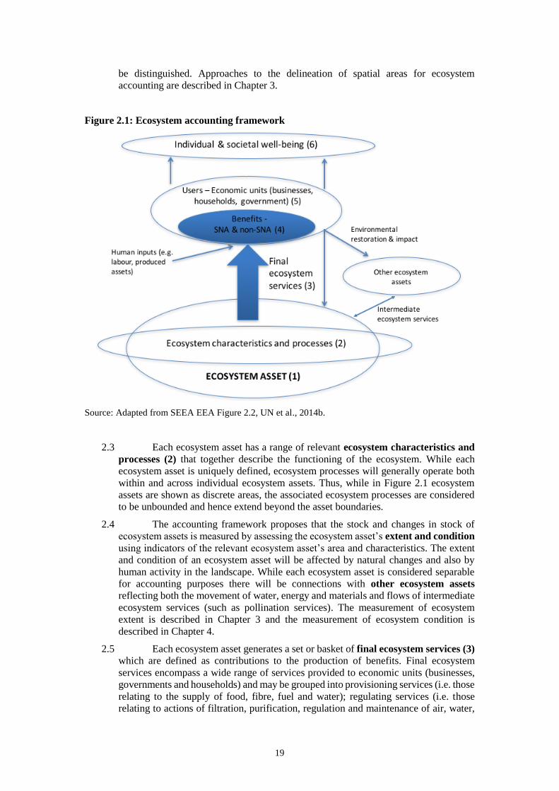
19

be distinguished. Approaches to the delineation of spatial areas for ecosystem

accounting are described in Chapter 3.

Figure 2.1: Ecosystem accounting framework

Source: Adapted from SEEA EEA Figure 2.2, UN et al., 2014b.

2.3 Each ecosystem asset has a range of relevant ecosystem characteristics and

processes (2) that together describe the functioning of the ecosystem. While each

ecosystem asset is uniquely defined, ecosystem processes will generally operate both

within and across individual ecosystem assets. Thus, while in Figure 2.1 ecosystem

assets are shown as discrete areas, the associated ecosystem processes are considered

to be unbounded and hence extend beyond the asset boundaries.

2.4 The accounting framework proposes that the stock and changes in stock of

ecosystem assets is measured by assessing the ecosystem asset’s extent and condition

using indicators of the relevant ecosystem asset’s area and characteristics. The extent

and condition of an ecosystem asset will be affected by natural changes and also by

human activity in the landscape. While each ecosystem asset is considered separable

for accounting purposes there will be connections with other ecosystem assets

reflecting both the movement of water, energy and materials and flows of intermediate

ecosystem services (such as pollination services). The measurement of ecosystem

extent is described in Chapter 3 and the measurement of ecosystem condition is

described in Chapter 4.

2.5 Each ecosystem asset generates a set or basket of final ecosystem services (3)

which are defined as contributions to the production of benefits. Final ecosystem

services encompass a wide range of services provided to economic units (businesses,

governments and households) and may be grouped into provisioning services (i.e. those

relating to the supply of food, fibre, fuel and water); regulating services (i.e. those

relating to actions of filtration, purification, regulation and maintenance of air, water,

20

soil, habitat and climate) and cultural services (i.e. those relating to the activities of

individuals in, or associated with, nature).

2.6 Benefits (4) may be SNA benefits - goods or services (products) produced by

economic units (e.g. food, water, clothing, shelter, recreation) currently included in the

economic production boundary of the SNA; or non-SNA benefits – benefits that accrue

to individuals, or society generally, that are not produced by economic units (e.g. clean

air). By convention, the measurement scope of non-SNA benefits for ecosystem

accounting purposes is limited to the flow of ecosystem services with a direct link to

human well-being.

2.7 In the accounting system, for each supply of final ecosystem services there is

a corresponding use that leads to the production of either an SNA or non-SNA benefit.

Further, in each sequence of use of ecosystem services and production of benefits there

is an associated user (5) being an economic unit – business, government or household.

Thus, every final ecosystem service flow represents an exchange between an ecosystem

asset (as a producing/supplying unit in the accounting system) and an economic unit.

Both SNA and non-SNA benefits contribute to individual and societal well-being (6).

2.8 The measurement of ecosystem services in physical terms is described in

Chapter 5 and the valuation of ecosystem services is described in Chapter 6. Ecosystem

accounting does not focus on the measurement of individual or societal well-being. It

is noted however, that in some decision-making contexts there may be direct interest

in the assessment of well-being and the choice of valuation approach may be varied to

take this in account. While the ecosystem accounts do not present valuations of well-

being and welfare change, the ecosystem accounting framework provides information,

particularly biophysical information, that is relevant to this form of analysis.

2.9 A key motivation for ecosystem accounting is to understand the potential for

ecosystem assets to provide services into the future and hence contribute to sustainable

overall individual and social well-being. In this context, the scientific literature on

ecosystem accounting has proposed four concepts in relation to ecosystem services

(Hein et al., 2016, building upon among others Bagstad et al., 2014 and Schröter et al.,

2014). These are: (i) the actual flow of ecosystem services, as recorded in the ecosystem

services supply and use account; (ii) the capacity of ecosystems to supply services,

corresponding to the sustainable flow of services subject to there being demand for

such services (flow equals capacity for regulating services); (iii) the potential supply

of services, indicating the potential, sustainable flow of services assuming no

limitations in demand for the service (hence potential flow is a function of ecosystem

characteristics only, it is not influenced by the presence of people using the service);

and (iv) ecosystem capability, reflecting the ability of the ecosystem to generate

services if it where managed in a different way. Potential supply and capability are

concepts that are relevant for environmental management, and less so for accounting

(although it can be noted that condition accounts are most directly linked to the

potential of the ecosystem to supply services rather than to the actual service supply

that also depends upon human use of the ecosystem). These concepts are further

discussed in Chapter 7.

2.10 Finally, the aggregate contribution and role of all ecosystem assets will be

relevant in understanding national level changes in wealth and associated concepts of

sustainability. The integration of information on ecosystem assets and services with

data from the SNA accounts is described in Chapter 8.

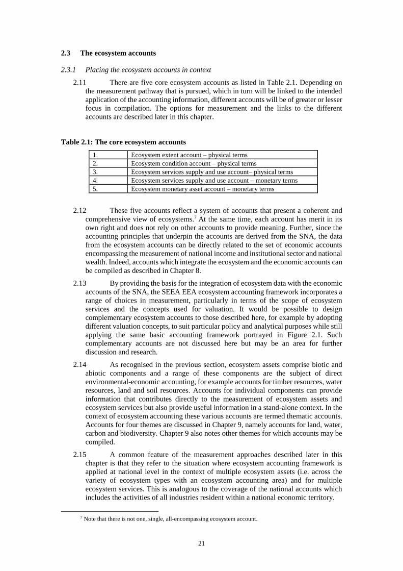
21

2.3 The ecosystem accounts

2.3.1 Placing the ecosystem accounts in context

2.11 There are five core ecosystem accounts as listed in Table 2.1. Depending on

the measurement pathway that is pursued, which in turn will be linked to the intended

application of the accounting information, different accounts will be of greater or lesser

focus in compilation. The options for measurement and the links to the different

accounts are described later in this chapter.

Table 2.1: The core ecosystem accounts

1. Ecosystem extent account – physical terms

2. Ecosystem condition account – physical terms

3. Ecosystem services supply and use account– physical terms

4. Ecosystem services supply and use account – monetary terms

5. Ecosystem monetary asset account – monetary terms

2.12 These five accounts reflect a system of accounts that present a coherent and

comprehensive view of ecosystems.7 At the same time, each account has merit in its

own right and does not rely on other accounts to provide meaning. Further, since the

accounting principles that underpin the accounts are derived from the SNA, the data

from the ecosystem accounts can be directly related to the set of economic accounts

encompassing the measurement of national income and institutional sector and national

wealth. Indeed, accounts which integrate the ecosystem and the economic accounts can

be compiled as described in Chapter 8.

2.13 By providing the basis for the integration of ecosystem data with the economic

accounts of the SNA, the SEEA EEA ecosystem accounting framework incorporates a

range of choices in measurement, particularly in terms of the scope of ecosystem

services and the concepts used for valuation. It would be possible to design

complementary ecosystem accounts to those described here, for example by adopting

different valuation concepts, to suit particular policy and analytical purposes while still

applying the same basic accounting framework portrayed in Figure 2.1. Such

complementary accounts are not discussed here but may be an area for further

discussion and research.

2.14 As recognised in the previous section, ecosystem assets comprise biotic and

abiotic components and a range of these components are the subject of direct

environmental-economic accounting, for example accounts for timber resources, water

resources, land and soil resources. Accounts for individual components can provide

information that contributes directly to the measurement of ecosystem assets and

ecosystem services but also provide useful information in a stand-alone context. In the

context of ecosystem accounting these various accounts are termed thematic accounts.

Accounts for four themes are discussed in Chapter 9, namely accounts for land, water,

carbon and biodiversity. Chapter 9 also notes other themes for which accounts may be

compiled.

2.15 A common feature of the measurement approaches described later in this

chapter is that they refer to the situation where ecosystem accounting framework is

applied at national level in the context of multiple ecosystem assets (i.e. across the

variety of ecosystem types with an ecosystem accounting area) and for multiple

ecosystem services. This is analogous to the coverage of the national accounts which

includes the activities of all industries resident within a national economic territory.

7 Note that there is not one, single, all-encompassing ecosystem account.

22

2.16 However, it is recognised that the ecosystem accounting framework may also

be applied with a more tailored focus. For example, the framework may also be applied

for measurement of:

• A single ecosystem asset or ecosystem type (e.g. a forest/s) and/or a single

ecosystem service (e.g. water regulation). For individual provisioning

services there may be a direct connection to natural resource accounting

described in the SEEA Central Framework Chapter 5.

• A single ecosystem asset or ecosystem type and multiple ecosystem

services. Accounting at this scale may be of interest in the management of

specific ecosystems or ecosystem types (e.g. wetlands).

• Multiple ecosystem types and single ecosystem services. Accounting of

this type may be of interest to understand the supply of a specific service

across a broad spatial area (e.g. water regulation, carbon sequestration).

• Areas of land within a country that have common land use or management

arrangements in place (e.g. national parks and protected areas).

2.17 In all of these “reduced” or tailored cases, the logic of the ecosystem

accounting framework described above can be applied. Indeed, to the extent that

individual projects focus on these more tailored accounts, it should be possible to

integrate the findings within a broader project covering multiple ecosystem assets and

services. Of course, the potential for integration lies heavily in the various projects

adopting consistent measurement boundaries and classifications but therein lies a prime

motivation for application of a common ecosystem accounting framework.

2.18 Another tailored application of ecosystem accounting is to focus on accounts

for regions within a country. This may include accounts at sub-national administrative

levels or for well-defined ecological areas (e.g. water catchments). Further, accounts at

a multi-country level (e.g. all European Union countries) can be envisaged. Again, the

ecosystem accounting framework can be applied at these different spatial levels.

2.19 In most instances, a staged approach to development of ecosystem accounts

should be considered most effective. Typically, an initial set of accounts including an

ecosystem extent account, condition account and ecosystem services supply and use

account for a single year would be compiled. An initial development phase may take

between one and two years. Depending on the initial scope, extension to develop

accounts could involve developing accounts for a larger set of services and condition

indicators, undertaking valuation of ecosystem services, compiling an ecosystem

monetary asset account and developing a time series of accounts. This should be

undertaken as an iterative process in which ongoing releases of accounting information

incorporate successive improvements in the accounts and underlying sources and

methods. The rate of progress will depend on a range of factors including the available

resources, complexity of account design (e.g. number of ecosystem types and

ecosystem services), data availability, the degree of experience with spatial analysis of

ecosystems and ecosystem services and the extent of collaboration between relevant

agencies that can be achieved.

2.3.2 Ecosystem extent accounts

2.20 The common starting point for all ecosystem accounting work will be

organizing information on the extent or area of different ecosystem types within a

country. This is important for four reasons. First, the task of defining the ecosystems

of interest for accounting purposes is by no means straightforward and a balance

between scale of analysis, available data and policy questions will need to be found. It

23

is very appropriate to start this discussion by examining the definition of ecosystem

assets and the delineation of their extent.

2.21 Second, the organisation of information required to establish an ecosystem

extent account will provide the basis for subsequent measurement of ecosystem

condition and many ecosystem services since indicators will generally vary by

ecosystem type.

2.22 Third, the structure of the ecosystem extent account, as shown below, gives a

clear indication of the nature of accounting for assets in a SEEA context. The

requirement to produce a time series of data to allow meaningful comparison between

the opening and closing of an accounting period is clear.

2.23 Fourth, while the ecosystem extent account provides a clear base for the

development of the other ecosystem accounts, it also provides important information

in its own right. For example, when compiled at appropriate levels of detail, ecosystem

extent accounts provide a common basis for discussion among stakeholders of the

composition of ecosystem types within a country and provide an assessment of

ecosystem diversity at a national level. Extent accounts can also support the derivation

of indicators of deforestation, desertification, urbanisation and other forms of land use

driven change.

2.24 The structure of the basic ecosystem extent account and relevant data sources

are described in Chapter 3.

2.3.3 Ecosystem condition accounts

2.25 A central feature of ecosystem accounting is organizing biophysical

information on the condition of different ecosystem assets across the area for which the

ecosystem accounts are produced (the 'Ecosystem Accounting Area' or EAA). The

condition account provides insight in how ecosystems within the EAA change, and

how those changes may influence the flows of ecosystem services supplied by those

ecosystems. The ecosystem condition account is compiled in physical terms using a

variety of indicators for selected characteristics. The structure of the ecosystem

condition account is described in Chapter 4.

2.26 Generally, it will be relevant to compile condition accounts by ecosystem type

within the EAA. This is because each ecosystem type (e.g. forests, grasslands,

wetlands, etc.) will have distinct characteristics that should be taken into account in

assessing condition. This measurement approach also recognizes that much

information on ecosystem condition is available by ecosystem type rather than in

reference to specific ecosystem assets (although such data may also be available and

should be utilized where possible).

2.3.4 Ecosystem services supply and use accounts

2.27 The supply of ecosystem services by ecosystem assets and the use of these

services by economic units, including households, is one of the central features of

ecosystem accounting. These are the flows that reflect the link between ecosystem

assets and economic and human activity. The supply and use account records the actual

flows of ecosystem services supplied by ecosystem assets and used by economic units

during an accounting period and may be compiled in both physical and monetary terms.

An extensive discussion of the ecosystem services supply and use account is in Chapter

5.

24

2.3.5 Ecosystem monetary asset account

2.28 Asset accounts are designed to record information on stocks and changes in

stocks (additions and reductions) of ecosystem assets. This includes accounting for

ecosystem degradation. The ecosystem monetary asset account records this

information in monetary terms, based on valuation of ecosystem services and

connecting to information ecosystem extent and condition. The ecosystem monetary

asset is described in Chapter 7.

2.3.6 Related accounts and concepts

2.29 The set of ecosystem accounts just summarised above reflects a complete

accounting coverage for all ecosystem assets and ecosystem services within a given

ecosystem accounting area in both physical and monetary terms. However, these

accounts and the information they contain cannot be considered in isolation. Two

connections to other accounts must be described.

2.30 The first connection concerns the integration of ecosystem accounting

information with the standard economic accounts, i.e. the compilation of integrated

ecosystem-economic accounts. The compilation of such accounts is relevant for the

derivation of degradation adjusted measurement of national income, the measurement

of national wealth in extended balance sheets, and to support the incorporation of

ecosystem services into extended input-output and other economic models and the

measurement of other macro-economic indicators such as environmentally-adjusted

measurement of multi-factor productivity. Issues associated with the compilation of

integrated ecosystem-economic accounts are described in Chapter 8.

2.31 Second, there are connections to the various accounts of the SEEA Central

Framework and similarly structured accounts for carbon and species-level

biodiversity8. The accounts of the SEEA Central Framework, as for carbon and species-

level biodiversity, focus on individual resources or flows such as water, timber, fish,

soil and land. Since these individual components are present within ecosystems, from

an accounting perspective, there must be a consistency in the picture presented between

these individual or thematic accounts on the one hand, and the ecosystem accounts on

the other.

2.32 Four key thematic accounts are described in Chapter 9 being for land, water,

carbon and species-level biodiversity. The information from these accounts will be of

direct relevance in the compilation of ecosystem accounts, particularly from the

perspective of supporting consistency in measurement across different ecosystem

types, for example by providing a broad framework for the integration of information

on stocks and flows of water resources. In addition, the information in each of the

thematic accounts is also likely to be of direct relevance in supporting discussion for

specific policy themes including land management and planning, water resource

management, management of carbon stocks and greenhouse gas (GHG) emissions and

biodiversity.

2.33 In addition, to these two accounting connections, an important concept not

portrayed directly in the set of ecosystem accounts listed above is ecosystem capacity.

Ecosystem capacity reflects the ability of an ecosystem to sustainably generate an

ecosystem service under certain assumptions (see section 7.3 for details). It underpins

the measurement of the valuation of ecosystem assets since the asset life of an

ecosystem will be directly related to changes in its capacity. In effect, the concept of

8 Following the CBD definition, biodiversity can be considered in terms of genetic, species and ecosystem

diversity. The assessment of ecosystem diversity is supported by the compilation of ecosystem extent

accounts. Genetic diversity has not been a focus of ecosystem accounting to this point.

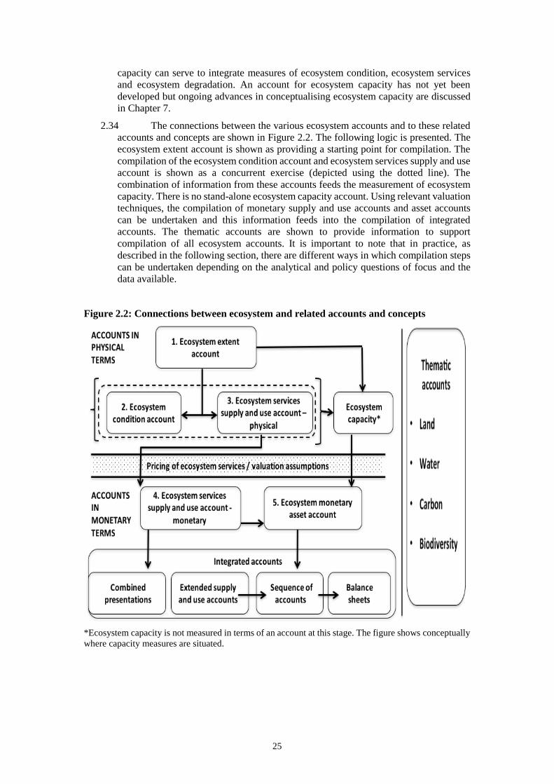
25

capacity can serve to integrate measures of ecosystem condition, ecosystem services

and ecosystem degradation. An account for ecosystem capacity has not yet been

developed but ongoing advances in conceptualising ecosystem capacity are discussed

in Chapter 7.

2.34 The connections between the various ecosystem accounts and to these related

accounts and concepts are shown in Figure 2.2. The following logic is presented. The

ecosystem extent account is shown as providing a starting point for compilation. The

compilation of the ecosystem condition account and ecosystem services supply and use

account is shown as a concurrent exercise (depicted using the dotted line). The

combination of information from these accounts feeds the measurement of ecosystem

capacity. There is no stand-alone ecosystem capacity account. Using relevant valuation

techniques, the compilation of monetary supply and use accounts and asset accounts

can be undertaken and this information feeds into the compilation of integrated

accounts. The thematic accounts are shown to provide information to support

compilation of all ecosystem accounts. It is important to note that in practice, as

described in the following section, there are different ways in which compilation steps

can be undertaken depending on the analytical and policy questions of focus and the

data available.

Figure 2.2: Connections between ecosystem and related accounts and concepts

*Ecosystem capacity is not measured in terms of an account at this stage. The figure shows conceptually

where capacity measures are situated.

26

2.4 The steps in compiling ecosystem accounts

2.4.1 Introduction

2.35 Ecosystem accounts can provide information that is relevant in a range of

policy and analytical contexts. However, in the initial development and testing phase,

it will likely be necessary to understand a more limited number of specific purposes or

questions for which ecosystem accounts might be compiled. The type of policy

question will help determine the scale of the accounts, either national or sub-national

(e.g. water catchment, province, habitat type, etc.), and the type of data needed. Over

time, and building on the initial testing, the development of a more complete set of

national level ecosystem accounts can be envisaged through progressive development,

extension and integration. Further, the development of an initial set of ecosystem

accounts is likely to spark awareness of additional potential applications.

2.36 Determining the appropriate coverage and spatial detail for a set of ecosystem

accounts, including the specific accounts to be compiled, must be a matter of discussion

among the institutions involved in compiling the accounts. It will also be necessary to

determine the relevant reference period/s for the accounts. Multiple data sources will

need to be brought together to compile the accounts and hence methods of adjusting

different source data to a common reference period/s will need to be adopted.

2.37 It is anticipated that the content of the Technical Recommendations will

support the discussion required to make these choices, although it is recognised that

other factors (such as the availability of resources) will need to be taken into account.

Following the general principles of SEEA implementation (see SEEA Implementation

Guide (UNSD, 2013)), the discussions should involve all relevant stakeholders,

including policy makers, data analysts, account compilers and source data holders.

These discussions can be very usefully supported by diagnostic tools that have been

developed for such purposes.9 As well, there can be significant benefits in establishing

a senior level steering committee and associated multi-stakeholder working or

technical groups. Note that the information in the Technical Recommendations is

appropriate for discussions on both the commencement of pilot studies and the

establishment of national programs of work.

2.38 The conceptual framework for ecosystem accounting shown in Figure 2.1

provides a general description of the relationships between the different stocks and

flows, and the connections between the accounts shown in Figure 2.2 provide a sense

of the overall accounting picture. This section provides an overview of the steps

involved in compiling ecosystem accounts.

2.39 The broad steps in ecosystem accounting are shown in Figure 2.3. The first set

of steps involves accounting in physical terms and the second set of steps is in monetary

terms. While it is useful to see this sequencing, the reality of accounting is that there

will be multiple iterations through the accounts and further, that the precise starting

point may vary. These iterations will reflect both the use of multiple data sources and

the aim of providing a consistent picture from them. While ecosystem accounts are

unlikely to convey the full richness and complexity of ecosystem relationships, they

should provide a strong organising framework for considering the information as well

as providing the means of conveying the key messages for policy and analytical

discussion.

9 https://unstats.un.org/unsd/envaccounting/workshops/Mexcio_2015_eea/Session%2013%20-%20%20SE

EA-EEA%20-%20Diagnostic%20Tool%2029MAY15%20V3.pdf

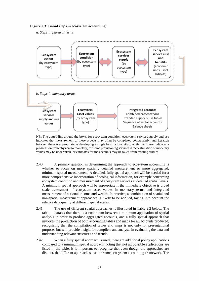
27

Figure 2.3: Broad steps in ecosystem accounting

a. Steps in physical terms

b. Steps in monetary terms

NB: The dotted line around the boxes for ecosystem condition, ecosystem services supply and use

indicates that measurement of these aspects may often be completed concurrently, and iteration

between them is appropriate in developing a single best picture. Also, while the figure indicates a

progression from physical to monetary, for some provisioning services direct estimation of monetary

values may be undertaken, or estimates for the accounts may be taken from existing studies.

2.40 A primary question in determining the approach to ecosystem accounting is

whether to focus on more spatially detailed measurement or more aggregated,

minimum spatial measurement. A detailed, fully spatial approach will be needed for a

more comprehensive incorporation of ecological information, for example concerning

ecosystem condition and measurement of ecosystem services at detailed spatial levels.

A minimum spatial approach will be appropriate if the immediate objective is broad

scale assessment of ecosystem asset values in monetary terms and integrated

measurement of national income and wealth. In practice, a combination of spatial and

non-spatial measurement approaches is likely to be applied, taking into account the

relative data quality at different spatial scales.

2.41 The use of different spatial approaches is illustrated in Table 2.2 below. The

table illustrates that there is a continuum between a minimum application of spatial

analysis in order to produce aggregated accounts, and a fully spatial approach that

involves the production of both accounting tables and maps for all accounts produced,

recognising that the compilation of tables and maps is not only for presentational

purposes but will provide insight for compilers and analysts in evaluating the data and

understanding relevant structures and trends.

2.42 When a fully spatial approach is used, there are additional policy applications

compared to a minimum spatial approach, noting that not all possible applications are

listed in the table. It is important to recognise that even though the approaches are

distinct, the different approaches use the same ecosystem accounting framework. The

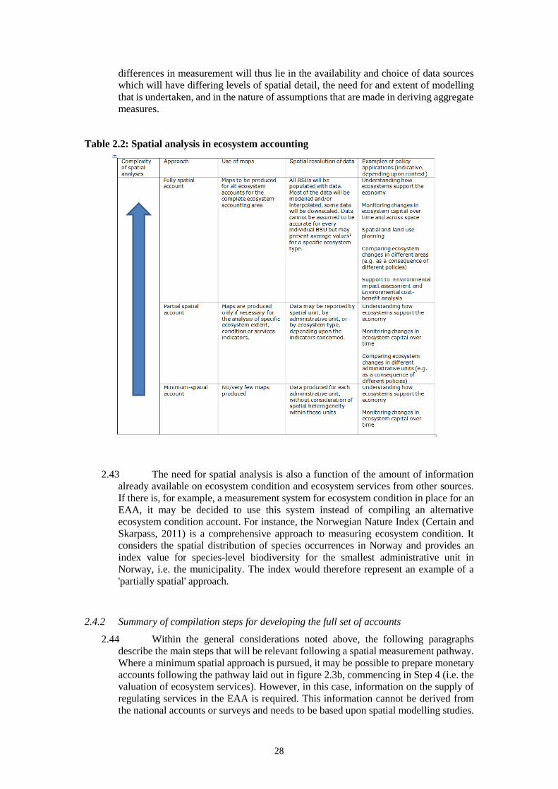
28

differences in measurement will thus lie in the availability and choice of data sources

which will have differing levels of spatial detail, the need for and extent of modelling

that is undertaken, and in the nature of assumptions that are made in deriving aggregate

measures.

Table 2.2: Spatial analysis in ecosystem accounting

2.43 The need for spatial analysis is also a function of the amount of information

already available on ecosystem condition and ecosystem services from other sources.

If there is, for example, a measurement system for ecosystem condition in place for an

EAA, it may be decided to use this system instead of compiling an alternative

ecosystem condition account. For instance, the Norwegian Nature Index (Certain and

Skarpass, 2011) is a comprehensive approach to measuring ecosystem condition. It

considers the spatial distribution of species occurrences in Norway and provides an

index value for species-level biodiversity for the smallest administrative unit in

Norway, i.e. the municipality. The index would therefore represent an example of a

'partially spatial' approach.

2.4.2 Summary of compilation steps for developing the full set of accounts

2.44 Within the general considerations noted above, the following paragraphs

describe the main steps that will be relevant following a spatial measurement pathway.

Where a minimum spatial approach is pursued, it may be possible to prepare monetary

accounts following the pathway laid out in figure 2.3b, commencing in Step 4 (i.e. the

valuation of ecosystem services). However, in this case, information on the supply of

regulating services in the EAA is required. This information cannot be derived from

the national accounts or surveys and needs to be based upon spatial modelling studies.

29

Estimates of the value of ecosystem assets (step 5) can in principal be obtained without

compiling ecosystem extent and condition accounts provided suitable assumptions are

made about the likely changes in the physical characteristics of ecosystem assets (e.g.

by assuming a fixed asset life).

2.45 Step 1: For ecosystem accounting, the first important step is to delineate the

area for which the accounts are compiled, the EAA. The EAA may cover the entirety

of a country’s land area (including inland waters) and, as appropriate, relevant coastal

and marine areas – perhaps extending to a country’s exclusive economic zone (EEZ).

Chapter 3 discusses the issues of delineating and classifying ecosystem assets for

ecosystem accounting purposes. Thought should also be given in this first phase to the

data infrastructure requirements noting that a fully spatial approach will be more

demanding in terms of computing capacity and data storage, as discussed in Chapter 3.

2.46 Information on the area of an EAA can be presented in an ecosystem extent

account. A key aim with this account is to measure the change over time in the

composition of ecosystem types within a country. The ecosystem extent account is

described in Chapter 3 and a discussion of the related land accounts is in Chapter 9.

2.47 Step 2: Using the listing of ecosystem types determined for the ecosystem

extent account, the next step is to compile the ecosystem condition account. Note that

this step may be undertaken following steps 3a and 3b and in any event, as indicated

by the dotted line in Figure 2.3, the measurement of ecosystem condition should take

into consideration relevant flows of ecosystem services. Chapter 4 discusses the

compilation of ecosystem condition accounts in more detail. Chapter 9 discusses the

compilation of information on land, carbon, water and biodiversity using accounting

approaches since these data may be relevant in monitoring the condition of many

ecosystems.

2.48 Step 3: The next step involves the measurement of ecosystem services in

physical terms.10 This is completed by considering each ecosystem service in turn and

determining the associated ecosystem types and appropriate indicators for

understanding supply and use. This task should be conducted using a classification of

ecosystem services, such as those described in Chapter 5. A classification can provide

a checklist to ensure appropriate coverage.

2.49 A common way of thinking about the supply of ecosystem services is to

imagine that each ecosystem type produces a specific basket of services in the same

way as a factory produces a set of outputs. This thinking is reflected in Figure 2.1. This

is certainly true for some ecosystem services, mainly provisioning services where

materials are harvested or extracted from a given ecosystem asset (e.g. timber from a

forest or water from a lake). However, for a number of ecosystem services, particularly

regulating services, the benefits derived arise through the effective “collaboration”

among different ecosystem types. For example, the regulation of water flows to provide

flood protection will involve contributions from forests, grasslands, and other

ecosystem types within a flood plain. While it is possible to estimate the contribution

of different ET to the provision of an individual service (e.g. the relative contribution

of forests to water regulation), the starting point for measurement is likely to be best

considered in terms of an individual service rather than a single ET.

2.50 Step 3 should encompass estimation of both the supply of ecosystem services

and the use of those services by various beneficiaries. Together, the information on

supply and use are used to compile an ecosystem services supply and use account.

To support integration with the national economic accounts, the beneficiaries in

10 In this context, “physical” means “non-monetary” and measurement in physical terms encompasses

ecosystem services that reflect flows of materials and energy, flows of services related to the regulation of

an ecosystem, and flows related to cultural services. (SEEA EEA para 3.2)

30

ecosystem accounting are grouped in the same way as for the economic accounts – i.e.

by industry group and by institutional sector. The possible approaches to measurement

are discussed in Chapter 5.

2.51 Step 4: Here the focus is on the valuation of ecosystem services in monetary

terms. There are many examples of the valuation of ecosystem services and it is a

necessary step for certain types of integration with the standard national accounts, such

as adjusted GDP and extended measures of net wealth. The valuation of ecosystem

services supports the compilation of ecosystem service supply and use account in

monetary terms and also the ecosystem monetary asset account and measures of

ecosystem degradation. The measurement of ecosystem degradation requires an

assessment of ecosystem capacity which reflects the connection between ecosystem

condition, ecosystem extent and ecosystem services.11 The valuation of ecosystem

services is discussed in Chapter 6 and the compilation of ecosystem monetary asset

accounts and estimation of ecosystem capacity is described in Chapter 7.

2.52 Step 5: The final step involves the use of information on ecosystem services,

ecosystem assets and ecosystem degradation from the accounts described above, to

integrate environmental and economic data and augment the current, standard national

accounts. As discussed in Chapter 8, this may be done in a number of ways including:

i. The compilation of combined presentations where data on ecosystem

condition and services in physical terms are presented alongside standard

economic data, such as value added, employment, or costs of

environmental restoration.

ii. The full extension of the ecosystem services supply and use accounts in

monetary terms to also include all products. This approach can be used to

show the integration of ecological and economic supply chains.

iii. The compilation of an extended sequence of accounts where standard

economic measures such as GDP, national income, and national saving are

adjusted for the cost of ecosystem degradation. Adjusted measures may

also be derived by institutional sector and industry.

iv. The estimation of a national balance sheet in which the value of ecosystem

assets is incorporated with the value of other assets and liabilities to derive

extended measures of national wealth.

2.53 In undertaking these different steps, under either fully spatial or minimum

spatial approaches to measurement, it should be understood that the logic of the

approaches is consistent with the types of approaches used for the compilation of

national accounts. National accounting measurement has some differences from many

statistical and scientific measurement approaches particularly concerning the

integration and confrontation of data. The key aspects of national accounting

approaches to measurement are summarised in Annex 2. This annex has been included

to provide an overview of the key elements of the national accounting approach that

underpins the compilation of ecosystem accounts described here. This material is

highly relevant to those who have not practised national accounting.

2.5 Key considerations in compiling ecosystem accounts

2.54 Six key considerations emerge in understanding the set of ecosystem accounts

as presented in the Technical Recommendations.

11 The measurement of ecosystem capacity may be facilitated by the description of baseline scenarios, i.e.,

describing expected changes in ecosystem condition given relevant business-as-usual assumptions.

31

2.55 First, as far as possible, the accounts are designed as a system of accounts such

that information can be readily compared between accounts. Thus, while there is more

than one account, and each account can stand alone, there are relationships between the

accounts that can be highlighted by structuring the information appropriately,

recognising that, in practice, the connections between ecosystem service flows and

ecosystem assets are difficult to define and measure.

2.56 Second, a very specific design feature of the ecosystem accounts is that

ultimately the information should be able to be integrated with the standard national

accounts that record economic activity. This design feature does not impact on all

accounts but is particularly relevant for accounts concerning ecosystem services and

accounts compiled in monetary terms.

2.57 Third, the accounting structures presented should not be considered

unchangeable with regard to the level of detail they contain. For example, the accounts

concerning ecosystem condition, described in detail in Chapter 4, are structured

according to broad ecosystem types (e.g. grasslands). In practice, it may be most

relevant to provide finer detail for some specific ecosystem types (e.g. by type of

grassland). Such rearrangements of information are perfectly appropriate and usually

necessary to ensure that the level of detail is determined based on analytical and policy

requirements and with regard to data availability.

2.58 Fourth, the accounts described in the Technical Recommendations present

information for one accounting period, usually one year. Most commonly, the interest

in accounting information stems from the presentation of time series of information,

i.e. for multiple accounting periods. The duration of an accounting period can be

altered, for example to develop sub-annual accounts which may be relevant for some

purposes such as seasonal analysis of ecosystem services related to water.

2.59 Presuming that a time series of accounts is compiled, users of accounting

information are likely to require a re-organisation of the information such that time is

one of the dimensions presented in the accounts. In practice, this is an issue of data

management and dissemination rather than of concept. Compilers should feel free to

restructure the accounts described here in such a way to best suit the presentation and

analysis of data, in reference to the associated policy questions and the needs of users.

2.60 Fifth, the structure of accounts will generally represent a level of detail suitable

for presentation and analysis of outputs from accounting. It represents the level of detail

at which accounting relationships (e.g. supply and use, balancing end of period stocks

and changes in stocks) are applied. However, it will generally be necessary for

underlying information to be organised at different, usually lower, levels of aggregation

before entry into the accounts.

2.61 In the case of ecosystem accounting, for spatial approaches it is likely to be

ideal to compile data at an appropriately detailed level using a common spatial data

infrastructure and then aggregate to the relevant ecosystem type level for accounting

purposes. This does not require that ecosystem accounts are compiled at fine levels of

detail but rather that the input (or source) data and the output (or disseminated) data are

managed distinctly.12 Indeed, making this distinction between input and output data is

essential if changes to the source of the input data are to be managed effectively without

affecting the integrity of the time series of data contained in the disseminated accounts.

Changes to input data, including changes to classifications, should be considered a

normal and common feature of accounts compilation.

12 The term “reported” data is commonly used. For most non-statisticians, this term relates to output or

disseminated data however for statisticians it relates to data collected or reported that is used to form

statistical estimates. Given the divergent use of the same term, it is not used in these Technical

Recommendations.

32

2.62 For some input data sources, detailed spatial information will be a feature, for

example for remote sensing and satellite based data. However, for most other input data

sources, the generation of detailed spatial data with coverage across relevant parts of

the ecosystem accounting area will require additional work. For data sourced from

official statistical sources, it would commonly be necessary to downscale aggregate

data using allocative techniques. The development of geo-referenced statistical

information may be a useful input to this process. For administrative data sources data

may be available for specified sub-national areas but adjustment may be needed to align

to ecosystem boundaries of interest. Again, geo-referencing of data is likely to be useful

in this task.

2.63 For information on environmental stocks and flows, many input data are

collected at specific locations and the challenge for ecosystem accounting is to

determine whether these data and associated relationships can be applied in other areas.

In the valuation of ecosystem services this task is termed “benefit transfer” but the

general principle of using specific observations and applying them to estimate values

for a broader population is applicable to all ecosystem measurement. Indeed, it is

standard practice in socio-economic surveys. The particular challenge for ecosystem

accounting is finding the correct levels of stratification of environmental features (e.g.

vegetation types, climate, elevation, etc.) such that observations can be appropriately

scaled. There is a range of approaches to benefit transfer for ecosystem measurement.

An introduction is provided in SEEA EEA Chapter 5 and there are several papers in

the scientific literature that provide further insights, such as Plummer (2009).

2.64 Sixth, a general ambition in the implementation of ecosystem accounting is to

facilitate the comparison of information on ecosystems within and between countries.

The ability to compare information can be an important basis for the discussion of

policy and can support analysis and data exchange. This is especially relevant with

respect to transboundary environmental stocks and flows such as water and migratory

species. The rationale for establishing comparability within ecosystem accounting is to

determine agreed measurement boundaries and definitions and associated

classifications, as reflected in an agreed ecosystem accounting framework. The focus

is not on ensuring that there is commonality in method, since differences in method

will likely be appropriate in different contexts.

2.65 At this stage in ecosystem accounting there is good progression towards an

agreed framework recognising of course that more discussion and testing is needed.

There is far less revealed agreement or commonality in methods for ecosystem

accounting. In part, this is due to the quite different applications of the ecosystem

accounting framework which naturally leads to the use of different methods and data

sources that are fit for purpose. It also reflects the breadth and variety of connections

between ecosystems and people that need to be taken into account.

2.66 With these points in mind, the ecosystem accounting framework described in

SEEA EEA, and as advanced in these Technical Recommendations, should be seen as

well-established and one that provides the basis for comparison and discussion. At the

same time, there is also considerable flexibility in the implementation of the

framework. Hence the methods discussed and the proposed structure of the different

ecosystem accounts should be taken as a guide to the types of information that can be

organized following an accounting logic. Countries are encouraged to compile

accounts using structures and methods that are most appropriate to understanding the

relationship between ecosystems and the economy in their country. Nonetheless, to

support ongoing dialogue and international comparison, it is essential that these

definitions, structures, classifications, concepts and resulting indicators are coherent

with the core framework presented in the Technical Recommendations. If variations

are used, these should be described and presented with the accounts.

33

2.67 The future design of ecosystem accounts will benefit from further testing and

discussion in terms of both the relevant compilation approaches and the most

appropriate levels for analysis and communication of results.

34

3 Organising spatial data and accounting for ecosystem extent

Key points in this chapter

Ecosystem accounting requires the delineation of areas within a country into mutually exclusive units

that represent ecosystem assets.

Ecosystem assets (EAs) are the distinct spatial areas that form the conceptual base for accounting and

the integration of relevant statistics. They represent contiguous areas covered by a specific ecosystem

(e.g. a single deciduous forest).

Ecosystem Types (ETs) are aggregations of individual EA of a specific type of ecosystem (e.g. deciduous

forests).

In the accounts, information may be reported by individual EA or by ET. Typically, when accounts are

developed at aggregated scales such as countries, the number of EAs is too large to meaningfully report

by individual EA, and accounts report information on ecosystem extent, ecosystem condition and

ecosystem services by ET.

Accounts will generally be produced for relatively large administrative areas, such as provinces, states

or countries; or in relation to large areas such as continents, bioregions or river basins that may cross

national boundaries. The area for which an account is produced is called the Ecosystem Accounting Area

(EAA). EAA are geographical aggregations of EAs that can be grouped by ETs.

Basic spatial units (BSU), in the form of grid squares or small polygons, support the delineation of EAs

and ETs and the organisation of spatial data sets for ecosystem accounting. For measurement purposes,

BSUs are assumed to be internally homogenous in terms of their biophysical properties.

Producing the accounts requires data on, for instance, topography, vegetation, land use and hydrology.

In a fully spatial approach, all spatial datasets should be brought together in a consistent way using the

same reference coordinate system within a common spatial data infrastructure.

A key bottleneck to producing accounts is getting access to different datasets, both spatial and non-

spatial, and integrating these data effectively. It is therefore important that collaboration is sought with

the various agencies holding datasets required for the production of the accounts. This may be time-

consuming and should be pursued in an early phase of account development.

3.1 Introduction

3.1. To provide a starting point for measurement, the SEEA EEA applies the

definition of ecosystems from the Convention on Biological Diversity (CBD) –

“ecosystems are a dynamic complex of plant, animal and micro-organism communities

and their non-living environment interacting as a functional unit” (CBD, 1992, Article

2, Use of Terms). Ecosystems are not straightforward to delineate spatially for

measurement purposes. In ecological terms, they may be defined at a range of spatial

scales, and hence it is often difficult to identify clear boundaries and they may overlap

in spatial terms. For statistical and accounting purposes, it is necessary to clearly

differentiate ecosystem assets as discrete units. Hence, the boundaries described here

should be considered a statistical abstraction from an ecological reality.

3.2. Ideally, in ecosystem accounting, all ecosystems within the area for which the

accounts are developed should be included. Urban areas, including sealed surfaces

should also be identified, even though they may have very few plant and animal species

and may provide relatively few ecosystem services. Where the accounts include entries

for types of ecosystems, the different ecosystems need to be delineated such that there

are no gaps or overlaps – i.e. the approach must be mutually exclusive and collectively

exhaustive.

3.3. A framework covering three types of spatial areas has been developed to allow

the organization of information into separate entities that can then be compared and

aggregated. This is akin to the role of a units model in economic statistics where

35

economic units (businesses, households and governments) are distinguished by their

types of economic activity and legal structure. These economic units can then be

grouped into relevant types, such as industry classes and institutional sectors.

3.4. This chapter outlines the approach taken in SEEA EEA to organise spatial data

and account for ecosystem extent, building on the discussion in SEEA EEA (Section

2.3). The framework for delineating spatial areas for ecosystem accounting is presented

in section 3.2 and section 3.3 describes the ecosystem extent account, and its role as

the basis for ecosystem accounting. Section 3.4 presents information on how the

ecosystem extent account can be compiled. The conceptual and practical aspects of

delineating spatial areas are described in section 3.5. In section 3.6 a summary of data

sources, classifications and methods is provided. Section 3.7 provides

recommendations for testing and areas for ongoing research.

3.5. The basic terminology and concepts related to spatial units are applicable to all

approaches to the implementation of ecosystem accounting. The difference is that in a

fully spatial approach a much larger set of information on ecosystems is mapped, while

in a minimum spatial approach, ecosystem services are only mapped and modelled

where this is required to obtain the information needed to fill the accounting tables.

3.6. In a fully spatial approach, where all ecosystem service flows and ecosystem

assets are mapped, the spatial infrastructure for ecosystem accounting may require

substantial data storage and computer processing power. For large countries, when

ecosystem accounting is pursued at high resolution, this requires powerful stand-alone

computers potentially with (some) data storage on internal or external (‘cloud’) servers.

Key considerations related to data handling and computing are provided in the sections

below.

3.2 The framework for delineating spatial areas for ecosystem accounting

3.2.1 Introduction

3.7. The conceptual framework for ecosystem accounting involves the integration

of data relating to three types of spatial units – ecosystem assets (EA), ecosystem types

(ET) and ecosystem accounting areas (EAA). These areas are key elements of the

ecosystem extent account and provide the basis for spatial analysis in the other

ecosystem accounts. Each of these three types of areas is described in this section (see

also Figure 3.1 below).

3.8. At this stage in the development of ecosystem accounting, considerable

flexibility is evident in the way in which these different areas may be delineated in

practice. Both relatively coarse and relatively fine delineations may be applied, for

example, linear landscape elements such as hedgerows may be distinguished as specific

ecosystem assets. Further, the criteria used to delineate ecosystem assets may be quite

varied, involving ecological factors only or also taking into account aspects of

ecosystem use and management.

3.9. At the same time, there are three principles that should underpin the definition

and delineation of spatial units for ecosystem accounting purposes. First, for a given

ecosystem accounting area (e.g. a country), the set of ecosystem assets should cover

the entire territory (i.e. all areas should be classified) and the spatial boundaries should

not overlap (i.e. the areas should be mutually exclusive). From a statistical and

accounting perspective, these requirements ensure that a complete and non-duplicative

picture can be described.

3.10. Second, the choice of spatial data and the associated classification of data that

are used to delineate spatial areas should be sufficiently detailed to be able to reflect a

36

composition of ecosystems across a country or EAA that is appropriate for analysis and

decision making. For example, if only a limited set of ecosystem types is applied then

it may only be possible to provide general messages of changes in ecosystems, while

with more ETs more detailed analysis might be developed.

3.11. Third, for a single set of ecosystem accounts (e.g. a set of extent, condition and

ecosystem services accounts) for a given ecosystem accounting area, the classification

of ecosystem types that is used should be common for the different ecosystem accounts

and any associated thematic accounts. Thus, for example, the area of wetlands reflected

in an ecosystem extent account should also underpin the measurement of the condition

of wetland areas and the measurement of ecosystem services related to wetlands. For

different sets of accounts within a country – e.g. a set of national level ecosystem

accounts and a set of ecosystem accounts developed for a specific area within a country,

such as an individual water catchment – areas may be classified in different ways since

the focus of accounting may be different. However, in these situations it will be

appropriate to adopt a correspondence of some sort.

3.12. The requirement for consistency across a set of accounts does not imply that

the delineated areas cannot change over time. Indeed, it would be expected that over

time, through the use of the same criteria, different boundaries would be delineated for

individual ecosystem assets to reflect their changing area, and accounting is designed

to record such changes. The second principle expects that these changes are

consistently reflected in all accounts for the same time point in the same way.

3.13. In describing a framework for the delineation of spatial areas it may appear as

though the task is a relatively linear one in that spatial areas are defined, measurements

are undertaken and then accounts are compiled. In practice, this linear sequence is

unlikely to be the case. Rather, particularly in the initial testing of ecosystem

accounting, it should be expected that a high degree of iteration takes place between (i)

the delineation of ecosystem assets, (ii) the classification of ecosystem types, (iii) and

the measurement of ecosystem condition and ecosystem services. Ultimately, a balance

will need to be found between the data available and the intended use of the data

building on an emerging understanding of the more relevant connections between

ecosystems and economic and human activity. This initial work will also highlight

those areas in which additional investment in data can add most value.

3.14. A stylised example of the spatial structure of the ecosystem extent account is

shown in Figure 3.1. The figure also shows the relationships between EA, ET and EAA.

The EAA is defined by the thick black boundary line. Six distinct EAs are delineated

and these have been classified to four different ET. The figure also incorporates the

basic spatial unit (BSU), the spatial unit of measurement, which is discussed in section

3.5. The BSU may correspond, as in Figure 3.1, to a grid cell in a spatial information

system or to individual polygons in cases where a vector based approach to ecosystem

extent accounting is pursued.

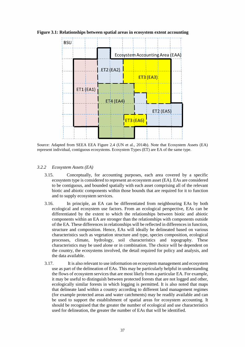
37

Figure 3.1: Relationships between spatial areas in ecosystem extent accounting

Source: Adapted from SEEA EEA Figure 2.4 (UN et al., 2014b). Note that Ecosystem Assets (EA)

represent individual, contiguous ecosystems. Ecosystem Types (ET) are EA of the same type.

3.2.2 Ecosystem Assets (EA)

3.15. Conceptually, for accounting purposes, each area covered by a specific

ecosystem type is considered to represent an ecosystem asset (EA). EAs are considered

to be contiguous, and bounded spatially with each asset comprising all of the relevant

biotic and abiotic components within those bounds that are required for it to function

and to supply ecosystem services.

3.16. In principle, an EA can be differentiated from neighbouring EAs by both

ecological and ecosystem use factors. From an ecological perspective, EAs can be

differentiated by the extent to which the relationships between biotic and abiotic

components within an EA are stronger than the relationships with components outside

of the EA. These differences in relationships will be reflected in differences in function,

structure and composition. Hence, EAs will ideally be delineated based on various

characteristics such as vegetation structure and type, species composition, ecological

processes, climate, hydrology, soil characteristics and topography. These

characteristics may be used alone or in combination. The choice will be dependent on

the country, the ecosystems involved, the detail required for policy and analysis, and

the data available.

3.17. It is also relevant to use information on ecosystem management and ecosystem

use as part of the delineation of EAs. This may be particularly helpful in understanding

the flows of ecosystem services that are most likely from a particular EA. For example,

it may be useful to distinguish between protected forests that are not logged and other,

ecologically similar forests in which logging is permitted. It is also noted that maps

that delineate land within a country according to different land management regimes

(for example protected areas and water catchments) may be readily available and can

be used to support the establishment of spatial areas for ecosystem accounting. It

should be recognised that the greater the number of ecological and use characteristics

used for delineation, the greater the number of EAs that will be identified.

38

3.18. If various data on ecological and use characteristics (as listed above) are not

available, a land cover based delineation of EAs may be used as a starting point. This

raises the practical question of which land cover classes should be considered and at

what level of detail. For EAs delineated based on land cover, it is recommended that

where possible, countries should use the most refined set of land cover types available

for their country to provide as close a match as possible with known ecosystem

typologies. Where country specific detail is not available, the most coarse level of

classification to be applied is the interim land cover classification of the SEEA Central

Framework which has 15 classes as shown in Table 3.1.13 Each of these 15 land cover

classes may be used to represent an ecosystem type, but should be further subdivided

into more detailed types where possible. Note that a class for sea and marine areas

should be incorporated to ensure appropriate coverage for all areas within the

Ecosystem Accounting Area.

3.19. Where an individual ecosystem crosses a national boundary, the associated

EAs need to be delineated with reference to the national boundary such that the

aggregate of all EAs for a country is equal to the total country area.

3.2.3 Ecosystem Type (ET)

3.20. EAs are contiguous areas representing individual ecosystems. In practice,

given that accounts are normally developed at aggregated scales, such as countries or

large water catchments, it may be difficult to analyse, record and report data for each

individual EA. It is therefore relevant to analyse accounting variables, such as

ecosystem condition and ecosystem service supply, at a more aggregated level

reflecting information for EAs of the same type.

3.21. For example, ecosystem account users may be interested in information on the

ecosystem services supplied by all EAs of type “deciduous forest”, rather than in

services from individual patches of deciduous forests. Alternatively, data may only be

sufficient to provide an estimate of the total supply of an ecosystem service for a

specific type of ecosystem, and hence cannot provide a meaningful indication of

service supply in each associated individual EA.

3.22. Accordingly, an ecosystem type (ET) is defined as a specific class of

ecosystem assets of comparable ecology and ecosystem use. Generally, across a

country, there will be a number of different areas (EAs) of the same ET. For example,

there may be different areas of (a type of) mangrove forest in different parts of a

country. Each individual mangrove forest is considered a separate EA but is classified

to the same ET.

3.23. Ecosystem types can be interpreted as aggregations of ecosystem assets of

similar type. As well, ecosystem assets can be interpreted as contiguous areas of a

specific ecosystem type. In practice, a ecosystem accountant will need to start with a

classification of ecosystem types in order to delineate ecosystem assets.

3.24. In defining ETs, it is helpful to consider the supply of ecosystem services, and

to aim for a high degree of commonality in ecosystem services supply within an ET.

For instance, grasslands located in floodplains provide an important hydrological

service (water storage leading to reduced flood risk) whereas grasslands located outside

13 The SEEA EEA proposed a set of 16 classes for land cover/ecosystem functional units. These classes were

developed as an application of the interim Land Cover classes presented in the SEEA Central Framework

by combining land cover information with information on land use. Since there may be various ways in

which land use and land cover information may be combined, it is now considered that for the task of

attributing land cover characteristics to EAs, the starting point should be the land cover classification of the

SEEA Central Framework. For a more detailed description of the land cover classes see the SEEA Central

Framework, Annex 1, Section C.

39

of floodplains do not provide this service. Thus, even though they have similar

vegetation cover, it is helpful to attribute these areas to different ETs, thereby

facilitating a coherent linkage between ET and ecosystem service supply. Similarly,

ecological detail concerning the type of perennial crop, or the hydrological properties

of a forest, facilitates identifying and analysing the ecosystem services supplied by

those ETs.

3.25. However, as the ecosystem type classification becomes more detailed, the

accuracy of the information used to identify them may reduce (depending on the data

source). In practice, a balance must be found between the number of different ETs that

are identified and the availability of information, noting that the use of a limited number

of types will also limit the sophistication of the questions that can be answered using

the accounting information.

3.26. In general, land use classifications are more specific (and have more classes)

compared to land cover classifications. In the same way, classifications of ET will

normally be more detailed than land use classifications (since in addition to land use

also the types of ecosystem services are considered; even with similar uses these

services may differ because of, e.g., hydrological properties as mentioned above).

3.27. Specifying ETs requires consideration of land cover, land/ecosystem use and

ecosystem services provided, the latter reflecting a function of natural vegetation,

institutional arrangements, location in the landscape, hydrology and/or soil type. At the

same time, the classification of ETs should not be prohibitively complex. It is

recommended to only consider selected (typically less than five) ecosystem services

and how they are supplied by different ecosystems in the classification of ETs based

on land use. For example, in low lying areas, services related to flood control may be

of high interest, in dry areas, services related to sustaining water flows may be of high

importance, and in mountains there may be areas that are essential for erosion control

(e.g. headwaters and riparian vegetation) that merit their inclusion as specific ET.

3.28. Table 3.1 provides an initial example of ET types and illustrates the difference

between land cover and ET. It shows that ETs are typically nested within land cover

classes thus recognising that differences in ecological characteristics are a prime

consideration in differentiating between ETs. Note as well that there is important

similarity between classes often defined in land use classifications and ETs. Generally,

only when land use classes provide distinctly different baskets of ES it is useful to

separate them into different ETs.

3.29. Experience to date with the development of ecosystem accounts for coastal

and marine areas is more limited. However, given that different marine areas provide

different ecosystem services, it will be appropriate to distinguish specific ecosystem

types within the land cover class ‘coastal ecosystem’ (e.g. seagrass meadow, coral reef,

oyster/mussel bank, mangrove, rocky substrate, sandy substrate, etc.). In the land cover

class ‘marine ecosystems’ there may be potential to differentiate between, for example,

reefs, sandbanks, continental shelf and deep sea.

3.30. There have also been, as yet, relatively few projects focusing on accounts for

urban ecosystems. Tentatively, it seems appropriate that in the case of urban

ecosystems various ecosystem types can also be differentiated based on the

combination of cover, use and the services they supply. This may include, for instance,

urban parks within city boundaries, different types of parks nearby cities but outside

residential zones, and perhaps even specific areas such as rivers flowing in urban areas,

river beds, canals or cemeteries.

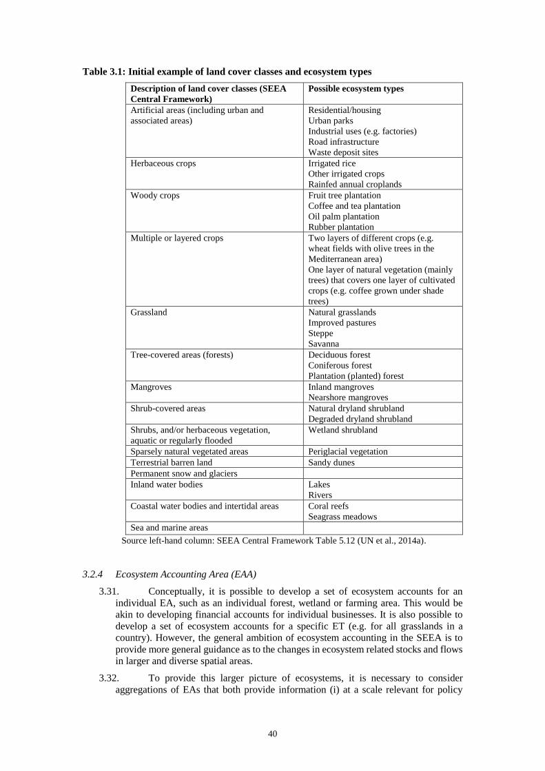
40

Table 3.1: Initial example of land cover classes and ecosystem types

Description of land cover classes (SEEA

Central Framework)

Possible ecosystem types

Artificial areas (including urban and

associated areas)

Residential/housing

Urban parks

Industrial uses (e.g. factories)

Road infrastructure

Waste deposit sites

Herbaceous crops Irrigated rice

Other irrigated crops

Rainfed annual croplands

Woody crops Fruit tree plantation

Coffee and tea plantation

Oil palm plantation

Rubber plantation

Multiple or layered crops Two layers of different crops (e.g.

wheat fields with olive trees in the

Mediterranean area)

One layer of natural vegetation (mainly

trees) that covers one layer of cultivated

crops (e.g. coffee grown under shade

trees)

Grassland Natural grasslands

Improved pastures

Steppe

Savanna

Tree-covered areas (forests) Deciduous forest

Coniferous forest

Plantation (planted) forest

Mangroves Inland mangroves

Nearshore mangroves

Shrub-covered areas Natural dryland shrubland

Degraded dryland shrubland

Shrubs, and/or herbaceous vegetation,

aquatic or regularly flooded

Wetland shrubland

Sparsely natural vegetated areas Periglacial vegetation

Terrestrial barren land Sandy dunes

Permanent snow and glaciers

Inland water bodies Lakes

Rivers

Coastal water bodies and intertidal areas Coral reefs

Seagrass meadows

Sea and marine areas

Source left-hand column: SEEA Central Framework Table 5.12 (UN et al., 2014a).

3.2.4 Ecosystem Accounting Area (EAA)

3.31. Conceptually, it is possible to develop a set of ecosystem accounts for an

individual EA, such as an individual forest, wetland or farming area. This would be

akin to developing financial accounts for individual businesses. It is also possible to

develop a set of ecosystem accounts for a specific ET (e.g. for all grasslands in a

country). However, the general ambition of ecosystem accounting in the SEEA is to

provide more general guidance as to the changes in ecosystem related stocks and flows

in larger and diverse spatial areas.

3.32. To provide this larger picture of ecosystems, it is necessary to consider

aggregations of EAs that both provide information (i) at a scale relevant for policy

41

monitoring and analysis; and (ii) at a scale where the accuracy of the information is

considered fit for purpose.

3.33. At the most aggregated levels, this involves accounting at the national or in

particular cases at the continental level14, i.e. covering all EAs within a country or group

of countries. However, it will commonly be appropriate to create aggregations of

i. EAs and ETs within specific sub-national administrative areas

ii. EAs and ETs within hydrologically defined areas within a country (such as

water catchments)

iii. other areas of policy interest such as protected areas, or areas owned by specific

industries or sectors, e.g. government owned land.

3.34. Commonly, these aggregations will reflect contiguous areas, such as

administrative areas or river basins, but this is not a requirement for accounting

purposes. The geographical aggregation for which the account is developed is labelled

the ecosystem accounting area (EAA).

3.35. Within each EAA there will be multiple EAs of different ETs, e.g. individual

EAs of forests, wetlands and cropland. The resulting accounting structures, as

introduced in Chapter 2, will generally be such that measures of ecosystem extent,

ecosystem condition and ecosystem services, will present information for aggregations

of EAs into ETs. For example, for a given sub-national administrative area, an

ecosystem extent account would show the changing total area of each ET (e.g. forest,

wetland, cropland). It would not show the changing area of each individual EA.

3.36. A single EA may be classified to multiple EAA, for example to an EAA formed

as using a water catchment and also to an EAA formed using an administrative region.

Incorporating a single EA into different EAA will be relevant depending on the

question being addressed.

3.3 The ecosystem extent account

3.37. The most common starting point for ecosystem accounting is organizing

information on the extent of different ecosystem types within a country in terms of

area. The structure of a basic ecosystem extent account is shown in Table 3.2. The

structure of the rows reflects the basic logic of asset accounts as described in the SEEA

Central Framework with an opening extent (in hectares or km2), closing extent,

additions and reductions. The columns reflect the chosen classification for ecosystem

types. The proposed structure here uses high level ecosystem types based on the interim

land cover classification in the SEEA Central Framework. Additional sub-classes may

be added depending on the ecosystem types of most relevance within a country. An

example of more detailed sub-classes is shown in Table 3.1 (above).

3.38. Where the type of land cover is the only characteristic used to delineate

different ecosystem assets, then a land cover account and an ecosystem extent account

will be the same. Where additional characteristics are used to delineate ecosystem

assets, different results would be expected.

14 As in the case of the European Union ‘KIP INCA’ project described in Annex 1.

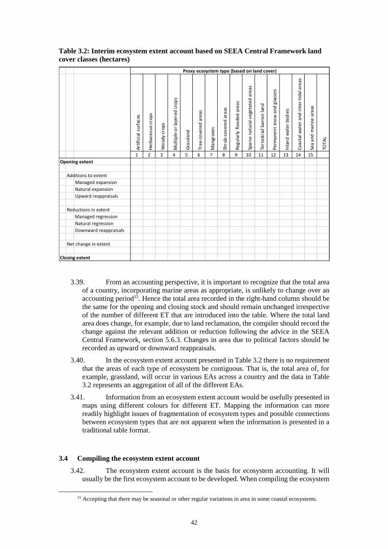
42

Table 3.2: Interim ecosystem extent account based on SEEA Central Framework land

cover classes (hectares)

3.39. From an accounting perspective, it is important to recognize that the total area

of a country, incorporating marine areas as appropriate, is unlikely to change over an

accounting period15. Hence the total area recorded in the right-hand column should be

the same for the opening and closing stock and should remain unchanged irrespective

of the number of different ET that are introduced into the table. Where the total land

area does change, for example, due to land reclamation, the compiler should record the

change against the relevant addition or reduction following the advice in the SEEA

Central Framework, section 5.6.3. Changes in area due to political factors should be

recorded as upward or downward reappraisals.

3.40. In the ecosystem extent account presented in Table 3.2 there is no requirement

that the areas of each type of ecosystem be contiguous. That is, the total area of, for

example, grassland, will occur in various EAs across a country and the data in Table

3.2 represents an aggregation of all of the different EAs.

3.41. Information from an ecosystem extent account would be usefully presented in

maps using different colours for different ET. Mapping the information can more

readily highlight issues of fragmentation of ecosystem types and possible connections

between ecosystem types that are not apparent when the information is presented in a

traditional table format.

3.4 Compiling the ecosystem extent account

3.42. The ecosystem extent account is the basis for ecosystem accounting. It will

usually be the first ecosystem account to be developed. When compiling the ecosystem

15 Accepting that there may be seasonal or other regular variations in area in some coastal ecosystems.

43

extent account the main challenges are to make informed choices on the ETs to be

distinguished and the resolution (and minimum mapping unit) of the maps. The starting

point will usually be the land cover, land use and ecosystem maps already available in

a country (or other area for which the accounts are to be produced) and the requirement

is to determine how information in these maps can be combined to produce an

ecosystem extent account and map that reflects the composition of ET. Based on these

information sets it needs to be decided if a raster or a vector based approach to

producing the ecosystem extent account is used, see also section 3.5 below.

3.43. In addition, in particular when accounts are produced for smaller areas, it may

be decided to fill the accounts with more detailed information for individual EAs. This

increases the resolution at which data on ecosystem services flows and assets needs to

be compiled.

3.44. The framework for delineating spatial areas described above focuses on

ecological characteristics, ecosystem use and ecosystem services. Further, since all data

layers will be connected to a common reference coordinate system, it is possible to

overlay different spatial information (data layers) in different ways for accounting

purposes.

3.45. In many countries, cadastres are well established, i.e. administratively defined

areas that are delineated on the basis of land ownership. Information from cadastre-

based datasets can be linked to information on EAs, ETs, economic activity, land use

and other socio-economic information. For instance, it is possible to combine

information on land ownership (tenure) with ET and water catchment information to

understand the ownership of ETs within each water catchment.

3.46. The use of cadastre-based information is likely to be meaningful in terms of

understanding the link to policy initiatives, particularly in those countries where land

is under private ownership. However, it is not recommended that land ownership data

be directly applied to delineate EA since this information may raise sensitivities in

many countries. Furthermore, depending upon the size of the cadastres, it may be

common for a single cadastre to comprise multiple EA.

3.5 Spatial infrastructure, measurement, and data layers

3.5.1 Basic spatial units (BSU)

3.47. While EA, ET and EAA represent the spatial areas for accounting and

statistical purposes, for many ecosystem measurement purposes there is a need for a

spatial measurement unit as a basis for constructing the accounts. For ecosystem

accounting, this spatial unit is termed a basic spatial unit (BSU). A BSU is a small

spatial area that is a geometrical construct. The purpose of BSUs is to provide a fine

level frame to which a range of different information can be attributed. The precise

definition of BSUs will depend on the context and the nature of the approach taken to

managing spatial data for accounting.

3.48. To develop a spatial data infrastructure for accounting, it is first necessary to

select and set-up a soft and hardware environment integrated into a Geographical

Information System (GIS). This will usually involve the use of a GIS software package

such as ArcGIS© or Quantum GIS. Adequate data storage and computing power are

also required.

3.49. Next, a specific reference coordinate system needs to be selected. Ecosystem

accounting relies on the integration of different spatial data sets or ‘layers’. It is

necessary that all spatial data layers, whether containing raster (grid) or vector data, are

converted to the same reference coordinate system for analysis. Countries generally

44

have a specific reference coordinate system, and the ecosystem accounts can use either

this system or a global reference coordinate system (such as WGS 84).

3.50. When global datasets are used to complement national data, it needs to be

verified that all datasets use the same reference coordinate system, and if not, spatial

data should be corrected for this (by using standard procedures in GIS involving the

connection of spatial data to the selected reference coordinate system).

3.51. Of relevance also, is the projection system that is used to transfer the three-

dimensional earth surface to a two-dimensional spatial data layer. When grid shaped

BSUs are part of the spatial data infrastructure, normally an equal area projection is

recommended in order to ensure that all grid cells have the same size.

3.52. With this infrastructure in place, the datasets to be used for the accounts can

be integrated in the selected spatial data environment. Typically, ecosystem accounting

involves the integration of data from national accounts, surveys and spatial data from

different sources (including from thematic maps and remote sensing data). Spatial data

is usually available at different resolutions (thematic maps often use polygons, remote

sensing data may be available at 30m grid (LandSat) or, increasingly, at 10m grid

(Sentinel 2)). In order to fill data gaps, where appropriate data can be interpolated and

extrapolated to establish wall-to-wall maps (i.e. no missing or undefined cells) of

relevant variables for the different accounts.

3.53. In defining BSUs and analysing spatial data, a flexible approach is proposed

in recognition of the large differences across countries in terms of spatial area,

ecological heterogeneity and data availability. A fundamental choice in setting up the

spatial data infrastructure is whether to use a reference grid and use this reference grid

to integrate all data layers, or to allow different datasets to have different formats (grid

or vector) and/or different grid sizes.

3.54. A reference grid approach should be understood as an approach where a

reference grid is established with single reference coordinate system and with an agreed

grid size, for example, 100 by 100m. Then, for all data layers, data are attributed to the

reference grid cells ensuring that for every data layer there is a specific value for each

reference grid cell. Such an approach has the advantage that it reduces the amount of

data involved and the complexity of the spatial modelling.

3.55. Where a reference grid is established, a key question is what size the grid

squares should be for ecosystem accounting purposes. There are three main

considerations in the selection of the grid size. First, the resolution at which data are

available. Second, the spatial variability of the ecosystems within the EAA. Third, the

potential limitations on computational capabilities and data storage. For example, an

EAA with many small landscape elements such as forest patches and hedgerows will

require a finer (smaller) grid compared to EAAs with large-scale landscape elements

such as large savannah areas.

3.56. In general, it can be recommended that grid sizes of 25 to 100m typically be

considered a good starting point for accounting purposes, but note that larger grid sizes

may be appropriate where accounting is undertaken at the continental scale. Grid sizes

down to 10m and smaller are now possible in some countries, but whether delineation

at that level of detail is required or appropriate for ecosystem accounting should be

informed by the use of the accounts for decision making. The use of a single reference

grid generally reduces the accuracy of (some of) the data. Further, the larger the grid

squares, the higher the inaccuracy that is introduced by converting individual data

layers to the reference grid.

3.57. Where a reference grid is established, each cell in the reference grid represents

a BSU. In this approach, a range of information is attributed to each BSU, including

45

for example details of EA, ET, land cover, soil type, elevation and other biophysical

and/or socio-economic information.

3.58. The alternative to using a reference grid, perhaps more appropriate for smaller

EAAs, is to include spatial datasets with different resolutions (for instance a

combination of relatively coarse vector-based thematic data, a more detailed vector-

based topographic dataset, ecosystem condition indicators sampled with remote

sensing imagery of 30m resolution and other ecosystem condition indicators sampled

at 10m resolution). Provided a consistent reference coordinate system is used for all

data layers, these different datasets can be used and integrated in the accounting

structure. An advantage of this approach is that there is no loss of information due to

the aggregation of datasets to a specific grid. However, depending on the number of

data layers that are combined the resulting intersecting areas may be small and

additional computational resources may be needed.

3.59. Where a reference grid is not used, the EAs and the ETs may be defined in the

ecosystem extent account either using a raster or a vector based approach. As noted,

this account is the basis for ecosystem accounting. A raster based ecosystem extent

map is usually the result of an analysis of remote sensing images, whereas an ecosystem

extent map based on a combination of topographic and thematic datasets will typically

be in vector format. Note that the use of a vector format is particularly relevant for the

analysis of linear and point elements in the landscape, in particular for elements which

may not be covered accurately using a raster map, such as roadsides, hedgerows,

streams or individual trees (in an urban context).

3.60. Further, where no reference grid is used, each data layer may have its own

specific resolution. In this case, the BSU represents the smallest spatial unit underlying

the ecosystem extent account, which as noted may either be in a raster on in a vector

format. Note that in a raster-based approach to ecosystem extent accounting, an EA

may be composed of one or a set of BSUs (of the same ET). In a vector-based

ecosystem extent account, the BSU corresponds to individual polygons (which are

likely to represent areas of different sizes). In a vector-based approach, typically, one

BSU represents one EA.

3.5.2 Data layers and delineation

3.61. The delineation of spatial areas and the analysis of ecosystem service flows

will involve the use of a range of spatial information including:

• Land cover and land use from either existing maps and referenced point

data or based on additional remote sensing imagery

• The topography of the country (coastline, digital elevation model (DEM),

slopes, river basins and drainage areas)

• Vegetation type and habitat type

• Species composition

• Hydrology (river and stream networks, lakes, groundwater flows and

aquifers)

• Soil resources and geological data

• Meteorological data

• Bathymetry (for coastal areas)

• Administrative boundaries

46

• Population, built-up areas and settlements

• Transport and communication (roads, railways, power lines, pipelines)

3.62. In some instances, data layers may have only been partially populated, i.e. the

spatial cover of the data does not extend to the full EAA, or it involves geo-referenced

point data rather than maps. In these cases, the unpopulated areas of each spatial layer

need to be classified as either “no data” or “unclassified’, or the missing data need to

be modelled or inter- and extrapolated, to ensure consistent coverage and reporting.

Various spatial interpolation tools such as inverse distance weighting, ‘kriging’ or

maximum entropy modelling may also be used for this, see for example Schröter et al.

(2015) or Willemen et al. (2015), as well as paragraph 3.74 below. The appropriate

approach for populating data layers should consider the type of data and experience of

experts in the specific measurement area.

3.63. With these data sources and tools in place, there is a range of choices available

for delineating the spatial units needed for ecosystem accounting, depending on scale

(i.e. the level of spatial detail) and thematic detail (the number of classes in the

classification). The following considerations are relevant, beyond those described in

section 3.2 and building on the discussion on BSUs above.

3.64. First, there is no standardised method for delineating EAs. However, it needs

to be considered that when the ecosystem accounts are developed for a (part of)

country, it is important to build upon existing environmental and other datasets. This

allows efficient use of available data, facilitates the integration of datasets and avoids

producing partially overlapping datasets. Countries will generally have land cover or

ecosystem type maps that can be used as a basis for preparing an ecosystem extent

account inclusive of a mutually exclusive and exhaustive definition and delineation of

EAs. Depending upon the EAA and the diversity of ET, the compilers of the ecosystem

accounts may decide to delineate individual EAs or instead work on the basis of ETs.

3.65. In delineating EAs, wherever possible, it is recommended that initial focus is

on ecological principles since EAs are considered the units that function to supply

ecosystem services. Habitat/biotope and vegetation classification methods are expected

to offer the most suitable inputs for delineation. However, as discussed above, it will

also be relevant to consider the services supplied by ecosystems in the delineation of

EAs. For example, in the Netherlands ecosystem extent account it was decided to

distinguish floodplains as an ET, given its importance in flood control and water

management. Flood plains may have similar land cover (mostly grasslands) as other

ETs (e.g. pastures), but the type was identified based on distinctive hydrology and

services supplied (i.e. water regulation).

3.66. For the integration of ecosystem information with socio-economic data, a

potential choice for EAA are nationally defined statistical areas. Statistical areas will

also commonly correspond best to the level of coverage of government decision-

making. Depending on the decision-making context, other boundaries will also be

relevant including state, province, municipality (specific data may be available from

national accounts for these administrative units), landscapes, water provisioning areas,

flood/storm protection areas and protected areas (e.g. national parks). Where statistical

data are not available at the desired spatial scale, methods for downscaling data will be

required.

47

3.6 Recommendations for developing a National Spatial Data Infrastructure (NSDI)

and the compilation of ecosystem extent accounts

3.6.1 Developing an NSDI

3.67. Based on the framework described in this chapter, a number of points emerge

as being steps that countries can focus on in testing and experimentation in ecosystem

accounting. A theme in these recommendations is that work to establish the spatial

areas required for ecosystem accounting is best undertaken within a broader context of

work, already completed or planned, to establish a national spatial data infrastructure

(NSDI) that would support integration of environmental and socio-economic data. The

INSPIRE project is an example of this type of direction (ref#). It should be recognised

that (i) an NSDI is not essential to commence work on the compilation of ecosystem

accounts and (ii) that there are many additional issues in the establishment of an NSDI

than presented here. In this broader context, the advances occurring through the UN

GGIM project are of particular importance as are numerous efforts underway at

national level (ref#).

3.68. The starting point in utilising an NSDI for ecosystem accounting is an

inventory of what spatial data infrastructure already exists in a country, in particular

within government agencies such as spatial planning or environmental agencies. This

assessment should include documenting the most commonly used GIS software

packages and the available datasets. Where feasible, the development of a spatial data

infrastructure for accounting should build upon existing infrastructure.

3.69. Relevant elements to consider in building upon an existing, or establishing a

new spatial data infrastructure include, but are not limited to, the coordinate and spatial

projection system, and whether a reference grid will be used. A reference grid may be

most relevant in case of large areas, large datasets, and restrictions in computing

capacity. If a reference grid is used, the size of the grid cells needs to be established.

Note that resolution is not equal to grid size. Resolution relates to the smallest objects

visible in an image or map, grid size is the on-the-ground area covered by a pixel.

Objects need to be larger than grid size to be visible in an image.

3.70. Another consideration in setting up the spatial data infrastructure is the

minimum mapping unit (MMU), i.e. the minimum size that a contiguous area needs to

have to be distinguished in the map. Usually, an MMU substantially exceeding the grid

size is chosen to facilitate interpretation of the map.

3.71. The development of spatial data infrastructure also requires selecting hardware

with sufficient processing, storage and back-up capacity, and GIS software.16

3.72. Within a spatial data infrastructure, integration of the following data layers is

recommended:

• Official boundaries, including country, administrative, statistical, river basins,

biogeographic areas, shorelines, etc. (as polygon vector data)

• Elevation and topography data, based on a digital elevation model (DEM). If no

detailed country-level data are available the global ASTER dataset17 can be used.

The DEM data are important to distinguish the elevation and slope of the BSU.

• Land cover data

• Additional data layers as available including

o Land management/use

16 Free and open source software, such as Quantum GIS, or commercial - ArcGIS 17 http://asterweb.jpl.nasa.gov/gdem.asp

48

o Vegetation type

o Soil and geology data

o Hydrological data related to rivers, lakes, streams, coastal and marine areas

o Data on urban infrastructure, including cities, villages, industrial zones,

and transport (rail, road), that is needed for assessing ecosystem condition

and understanding ecosystem use (e.g. relevant for mapping fragmentation

and other impacts)

• Socio-economic data including population data, employment, economic activity,

etc.

3.73. As part of the development of an NSDI and, ultimately a national register or

listing of ecosystem assets, it will be important to understand spatial areas that have

already been delineated by government agencies for administrative purposes, for

example land management areas, river basins and catchment management areas and

nature conservation/protected areas. In some cases, these existing spatial boundaries

may provide a suitable starting point for ecosystem accounting.

3.74. Further, it is appropriate to develop an understanding of the hierarchy of

ecosystem/landscape/eco-region/biome units that are relevant for the country. This can

be done in reference to existing products (e.g. World Wildlife Fund (WWF) eco-

regions, or the ESRI/USGS global ecosystems map

(https://rmgsc.cr.usgs.gov/ecosystems/). Overall, testing and experimentation should

reveal what are the most relevant data sources for the delineation of areas for ecosystem

accounting purposes while ensuring that the outcome provides a spatially exhaustive

coverage of a country.

3.75. It is important to recognise that the ecosystem accounting approach will be

most useful when developed over a period of time. Indeed, given the potential

complexity of the accounts, a step-by-step approach and learning by doing are required.

In addition, data will be more useful when both spatial and inter-temporal (trend)

analyses are possible.

3.76. A critical aspect in developing the accounts is the need to establish data sharing

arrangements and agree on data access with all the data holders. Data sharing and

capacity are the key bottlenecks, even more than the availability of data. It is

recommended that, given the amount of time it may take to establish data sharing

arrangements, this is one of the first priorities in the development of an NSDI. In the

development of the NSDI it is recommended to consider the data formats including the

reference coordinate systems used by the various agencies and to assess if similar

formats and coordinate systems can be aligned within an NSDI.

3.6.2 Recommendations for developing the ecosystem extent account

3.77. It is likely that in most cases, application of the SEEA EEA will start with

developing the extent account. The compilation of this account will be best conducted

using an NSDI. The key steps in developing a spatial data infrastructure for ecosystem

accounting are depicted in Figure 3.2 below. The figure shows that a first priority is to

establish objectives, priorities and a time path for the compilation of the accounts,

including the development of the NSDI, and then to select the ecosystem accounting

area for which the accounts will be developed. The ambition level of the account will

determine the relevant territory and the resolution at which data will need to be

generated. In turn, this will determine hardware and software requirements. Typically,

an initial pilot ecosystem accounting project may be run on an up-to-date, powerful,

stand-alone computer. However, if ecosystem accounting is applied for large countries

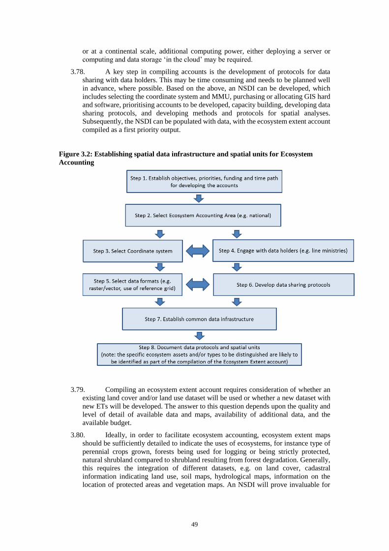
49

or at a continental scale, additional computing power, either deploying a server or

computing and data storage ‘in the cloud’ may be required.

3.78. A key step in compiling accounts is the development of protocols for data

sharing with data holders. This may be time consuming and needs to be planned well

in advance, where possible. Based on the above, an NSDI can be developed, which

includes selecting the coordinate system and MMU, purchasing or allocating GIS hard

and software, prioritising accounts to be developed, capacity building, developing data

sharing protocols, and developing methods and protocols for spatial analyses.

Subsequently, the NSDI can be populated with data, with the ecosystem extent account

compiled as a first priority output.

Figure 3.2: Establishing spatial data infrastructure and spatial units for Ecosystem

Accounting

3.79. Compiling an ecosystem extent account requires consideration of whether an

existing land cover and/or land use dataset will be used or whether a new dataset with

new ETs will be developed. The answer to this question depends upon the quality and

level of detail of available data and maps, availability of additional data, and the

available budget.

3.80. Ideally, in order to facilitate ecosystem accounting, ecosystem extent maps

should be sufficiently detailed to indicate the uses of ecosystems, for instance type of

perennial crops grown, forests being used for logging or being strictly protected,

natural shrubland compared to shrubland resulting from forest degradation. Generally,

this requires the integration of different datasets, e.g. on land cover, cadastral

information indicating land use, soil maps, hydrological maps, information on the

location of protected areas and vegetation maps. An NSDI will prove invaluable for

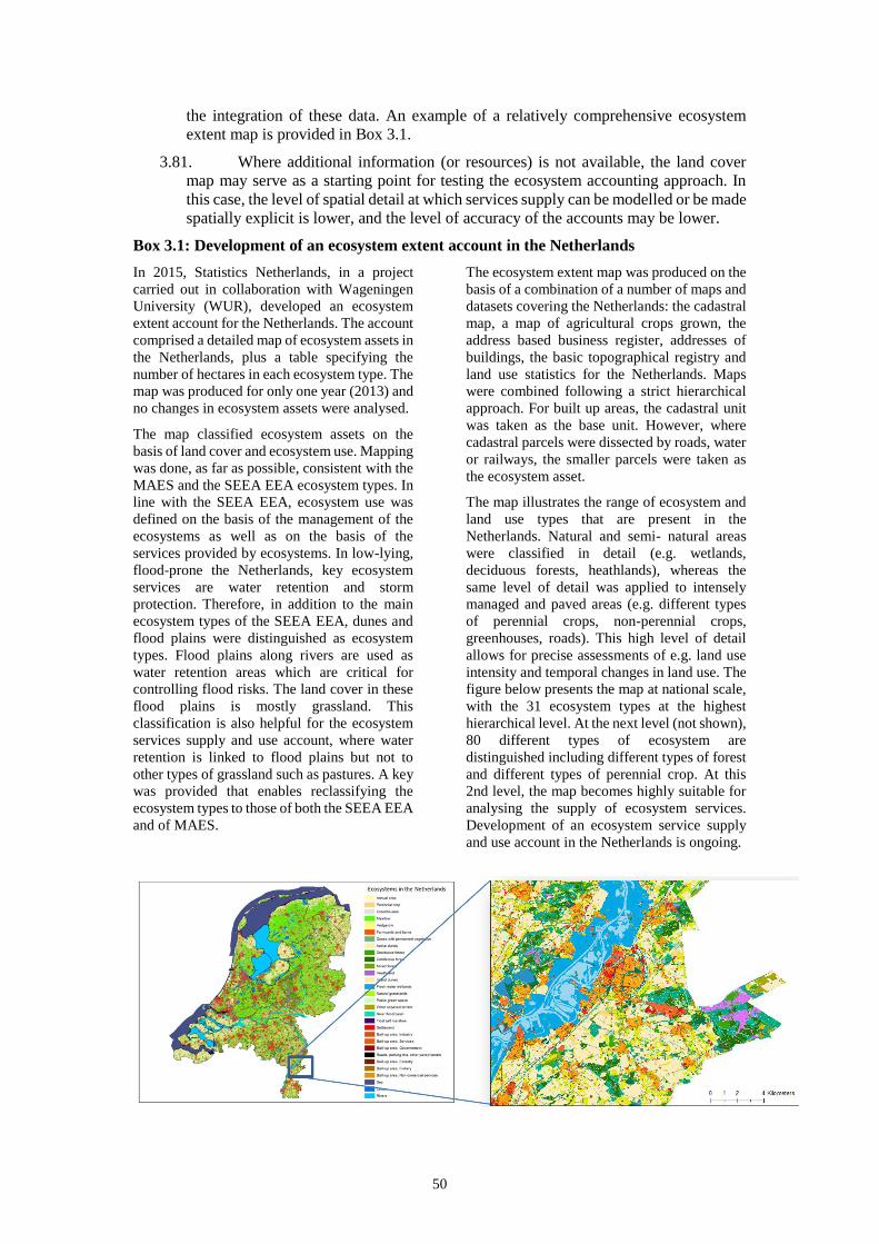
50

the integration of these data. An example of a relatively comprehensive ecosystem

extent map is provided in Box 3.1.

3.81. Where additional information (or resources) is not available, the land cover

map may serve as a starting point for testing the ecosystem accounting approach. In

this case, the level of spatial detail at which services supply can be modelled or be made

spatially explicit is lower, and the level of accuracy of the accounts may be lower.

Box 3.1: Development of an ecosystem extent account in the Netherlands

In 2015, Statistics Netherlands, in a project

carried out in collaboration with Wageningen

University (WUR), developed an ecosystem

extent account for the Netherlands. The account

comprised a detailed map of ecosystem assets in

the Netherlands, plus a table specifying the

number of hectares in each ecosystem type. The

map was produced for only one year (2013) and

no changes in ecosystem assets were analysed.

The map classified ecosystem assets on the

basis of land cover and ecosystem use. Mapping

was done, as far as possible, consistent with the

MAES and the SEEA EEA ecosystem types. In

line with the SEEA EEA, ecosystem use was

defined on the basis of the management of the

ecosystems as well as on the basis of the

services provided by ecosystems. In low-lying,

flood-prone the Netherlands, key ecosystem

services are water retention and storm

protection. Therefore, in addition to the main

ecosystem types of the SEEA EEA, dunes and

flood plains were distinguished as ecosystem

types. Flood plains along rivers are used as

water retention areas which are critical for

controlling flood risks. The land cover in these

flood plains is mostly grassland. This

classification is also helpful for the ecosystem

services supply and use account, where water

retention is linked to flood plains but not to

other types of grassland such as pastures. A key

was provided that enables reclassifying the

ecosystem types to those of both the SEEA EEA

and of MAES.

The ecosystem extent map was produced on the

basis of a combination of a number of maps and

datasets covering the Netherlands: the cadastral

map, a map of agricultural crops grown, the

address based business register, addresses of

buildings, the basic topographical registry and

land use statistics for the Netherlands. Maps

were combined following a strict hierarchical

approach. For built up areas, the cadastral unit

was taken as the base unit. However, where

cadastral parcels were dissected by roads, water

or railways, the smaller parcels were taken as

the ecosystem asset.

The map illustrates the range of ecosystem and

land use types that are present in the

Netherlands. Natural and semi- natural areas

were classified in detail (e.g. wetlands,

deciduous forests, heathlands), whereas the

same level of detail was applied to intensely

managed and paved areas (e.g. different types

of perennial crops, non-perennial crops,

greenhouses, roads). This high level of detail

allows for precise assessments of e.g. land use

intensity and temporal changes in land use. The

figure below presents the map at national scale,

with the 31 ecosystem types at the highest

hierarchical level. At the next level (not shown),

80 different types of ecosystem are

distinguished including different types of forest

and different types of perennial crop. At this

2nd level, the map becomes highly suitable for

analysing the supply of ecosystem services.

Development of an ecosystem service supply

and use account in the Netherlands is ongoing.

51

Source: CBS and WUR, 2015. Ecosystem Accounting Limburg Province, the Netherlands. Part I: Physical supply

and condition accounts. To download the full report: http://www.wur.nl/en/Expertise-Services/Chair-groups/Environmental-Sciences/Environmental-Systems-Analysis-Group/Research/Ecosystem-Services-and-Biodiversity/Ecosystem-Accounting.htm

3.7 Key research issues in delineating spatial areas for ecosystem accounting

3.82. Approaches to delineating spatial areas for ecosystem accounting are still

developing. There are four key research issues that can be identified.

3.83. First, fundamental to ecosystem accounting is the classification of EAs to ET

classes. At this time, definitive advice on the choice of classification, and the associated

level of detail, cannot be provided. In the first instance, as far as possible, countries

should seek to use relevant country specific classifications as these will reflect the local

situation. At the same time, ongoing research and discussion is needed to establish ET

classifications that support cross-country comparison and embody the principles of

ecosystem accounting.

3.84. Second, the framework including EA, ET and EAA has been developed in the

context of terrestrial areas. At the same time, there have been a range of studies

applying ecosystem accounting to coastal and marine areas. These studies include work

in South Africa (Driver et al., 2012), Canada (Statistics Canada, 2013), Mauritius

(Weber, 2014b), United Kingdom (UK) (UK ONS, 2016) and Australia (Australian

Bureau of Statistics, 2015)); and to river and freshwater systems (e.g. South Africa

(Driver, et al., 2012), Canada (Statistics Canada, 2013) and Australia (Victorian

Department of Sustainability and Environment, 2013). Further, the importance of

accounting for marine areas is well recognised and further research is required to fully

consider the spatial framework in these contexts.

3.85. Two specific challenges here are (i) to integrate the linear (usually vector-

based) datasets generally required for accounting for rivers with the datasets required

for terrestrial ecosystems; and (ii) to understand and include in the accounts the

interactions between terrestrial systems and river flows (such as the variation in water

flows throughout the year (through seasonality and extreme events), exchange of

nutrients between river and terrestrial ecosystems, etc.).18 The second challenge has

been captured in a range of hydrological modelling efforts, but this has seldom been

done at a scale (e.g. nation-wide) commensurate with scales typically considered in

accounting.

3.86. Third, further research is needed to appropriately incorporate some specific

ecological areas and aspects. This includes incorporation of information on soil

resources and their properties, linear features (such as hedgerows and roads) and

subterranean ecosystems (such as caves and groundwater systems). It also includes

areas not currently within scope of ecosystem accounting such as the atmosphere and

airsheds. With respect to the atmosphere a question is, for instance, whether it could be

included in the SEEA EEA as an ecosystem type which would then require delineation

vertically rather than horizontally. Interactions between the atmosphere and other

ecosystem types can in principle be quantified but there are as yet no examples of this

being tested.

3.87. Fourth, the delineation of spatial areas (as well as the compilation of the

condition and the physical ecosystem services supply and use accounts) may involve

the use of remote sensing data including satellite Earth Observation data. Where there

is an agreed national land cover map this should be utilised. Otherwise, there is an

increasing availability of such data including freely available data from MODIS (with

18 Some discussion of these issues is provided in SEEA Water in respect of the measurement of water quality.

52

medium spatial resolution since 2000, high temporal frequency and including derived

products such as land cover, vegetation dynamics and NPP), Landsat (several bands

(wavelengths) available at 30m grid since 1984 but with lower temporal frequency)

and, recently, Sentinel (including the Sentinel I radar sensor and the Sentinel II optical

sensor, with grid sizes of 10m for some bands of the optical sensor).

3.88. For each of these sources of satellite data there is a dedicated website where

images can be downloaded. Most images and products from MODIS and Landsat can

be accessed from (https://earthexplorer.usgs.gov/). Processing and interpretation of

images is required if the available products are not sufficient, as well as dealing with

issues such as cloud cover (for optical sensors). Further, there is the related challenge

of uncertainty in spatial interpretation and the need for validation and ground truthing

of the classified land cover, estimated NPP and other map products. These challenges

are not unique to ecosystem accounting but developing methods for adapting remote

sensing data for ecosystem accounting purposes is an important area for testing.

53

4 The ecosystem condition account

Key points in this chapter

“Ecosystem condition reflects the overall quality of an ecosystem asset in terms of its characteristics.”

(SEEA EEA 2.35). The measurement of ecosystem condition is a central aspect of ecosystem accounting

since it provides information on the capacity of ecosystems to provide ecosystem services into the future.

In general terms, ecosystem condition is measured by collating indicators for various ecosystem

characteristics for different ecosystem types. Within this broad framing there are different approaches to

the measurement of condition ranging from more aggregated to more detailed.

Generally, the development of indicators relating to characteristics such as vegetation, water, soil,

biomass, habitat and biodiversity for different ecosystem types, as well as indicators of relevant pressures

and drivers of ecosystem change, will be appropriate.

For some characteristics in certain ecosystem types, condition metrics are well established although

further testing is required to assess their use for ecosystem accounting. In other cases, the selection and

measurement of relevant characteristics is less established and measurement is more difficult.

A key challenge for ecosystem accounting is developing a full coverage of measures in a manner that

support aggregation and comparison. In particular, the establishment of composite indicators integrating

different condition parameters within different ecosystem types and ecosystem assets poses a core issue.

Reference condition approaches are one technique for developing measures that can be monitored over

time and can be compared across ecosystem types and across countries. Determining reference

conditions for multiple ecosystem types and more than one country is not straightforward and further

testing of relevant approaches for ecosystem accounting is required.

In advancing work on ecosystem condition measurement, it is essential that experts with knowledge of

local ecosystems are engaged to ensure the relevance of selected metrics and to take advantage of existing

monitoring and research.

4.1 Introduction

4.1 In the SEEA EEA, the general ambition in accounting for ecosystem condition

is to bring together the relevant pieces of information to provide an overall assessment

of the state or condition of various ecosystems in the ecosystem accounting area. The

general definition of ecosystem condition is provided in the SEEA EEA: “ecosystem

condition reflects the overall quality of an ecosystem asset in terms of its

characteristics.” (SEEA EEA, para 2.35).

4.2 The ecosystem condition account captures, in a set of key indicators, the state

or functioning of the ecosystem in relation to both its ecological condition and its

capacity to supply ecosystem services. The ecosystem condition account is

complementary to environmental monitoring systems in the sense that the condition

accounts organise aggregated, high-level information and indicators for an ecosystem

accounting area, and they typically integrate information from different environmental

monitoring systems (e.g. on biodiversity, water quality, soils, etc.). Hence, the

ecosystem condition account aims to builds upon and not replace information from

various monitoring systems. Compiling a comprehensive condition account will also

likely require collecting and analysing additional data (e.g. from remote sensing

images) and extrapolating or interpolating existing data.

4.3 The main benefit of compiling an ecosystem condition account lies in the

integration of different sets of information of ecosystem condition and in the

subsequent potential in the ecosystem accounting framework to combine this

information on ecosystem condition with information on ecosystem services flows and

monetary value of ecosystem assets. This integrated approach, using as a base a

common understanding of the size, composition and types of ecosystem assets, offers

54

a more comprehensive insight into changes in ecosystems compared to individual

datasets, thereby expanding the policy use of environmental information.

4.4 In the compilation of ecosystem condition accounts, a minimum, partial or

fully spatial approach can be pursued. In a minimum spatial approach, condition

indicators are compiled, aggregated and reported for the individual ETs within the

EAA. To a limited degree, spatial variability can be indicated by inserting minimum

and maximum values and standard deviations in tables, however this approach does

not allow assessment of condition at specific locations within the EAA. In the partial

spatial approach, some of the condition indicators may be spatially analysed and

combined with non-spatial indicators, and aggregated indicators may be reported by

ET or for administrative units. In a fully spatial approach, condition indicators are

comprehensively mapped, such as to provide values of condition indicators by EA. In

the fully spatial approach, accounting tables and maps are produced for all or the

majority of indicators so that spatial differences in ecosystem condition of EAs are

reflected in the accounts.

4.5 Indicators in the ecosystem condition account reflect the general ecological

state of an ecosystem, its capacity to supply ecosystem services and the relevant trends.

These indicators may reflect such aspects as the occurrence of species, soil

characteristics, water quality, and ecological processes (e.g. net primary production).

The indicators selected should be relevant for policy and decision making, for instance

because they reflect policy priorities (e.g. preservation of native habitat); pressures on

ecosystems (e.g. deposition levels of acidifying compounds versus critical loads for

such compounds) or the capacity of ecosystems to generate one or more services (e.g.

attractiveness of the ecosystem for tourism). Generally, different ecosystem types

require different indicators. For example, condition indicators relevant for forests will

be less relevant for cropland.

4.6 Basic spatial or non-spatial information about ecosystems that is commonly

needed for the measurement and modelling of ecosystem services supply, are not of

the highest priority for a basic condition account. For example, to model erosion risks

and the ecosystem service of erosion control, it is necessary to have information on,

among other things, rainfall, slope, slope length, and soil type for relevant ecosystem

assets. However, these indicators reflect ecosystem characteristics that do not generally

change rapidly over time and hence are not key indicators of the changing condition of

an ecosystem. Nonetheless, the collation and organisation of this information is likely

an important aspect in developing a complete database for ecosystem accounting, and

such information can be included in annexes to the ecosystem accounts.

4.7 Discussion since the release of SEEA EEA has highlighted the following

points that provide a broader context for the measurement of ecosystem condition.

4.8 First, the relevance of ecosystem condition indicators depends upon context.

In part, this reflects that the assessment of condition should take into consideration the

specific characteristics of the EAA including the ETs that are present, their

composition, and the likely uses of EAs. Data availability, or the possibility to obtain

additional data, are additional considerations in selecting condition indicators. Thus,

determining the appropriate set of characteristics is a particularly important task for

testing in ecosystem accounting. Recent discussion highlights that it should be possible

to give additional guidance as to the broad aspects that a set of indicators should cover

(e.g. habitat, pressures and drivers, biological responses, see also box 4.1) but this

requires further discussion in an accounting context.

4.9 Second, the types of indicators to be considered in the measurement of

ecosystem condition may include indicators that reflect pressures being exerted on

ecosystems. These may include, for example, air emissions, water effluents and the

55

production of solid wastes. These pressures may affect economic activities as well as

the condition of ecosystem assets.

4.10 Third, in some cases, it may be useful to compile composite indicators where

a range of indicators is combined to reflect different elements of ecosystem condition.

However, having determined a suitable set of indicators, there is no natural, a priori

weighting of the indicators that might be used to estimate the overall condition of an

ecosystem asset. Thus, a measure of the overall condition requires a view to be taken

on the relative importance of the different ecological processes involved, or the

different purposes for use of an ecosystem asset. It would be possible to give each

indicator equal weight, but this does not overcome the underlying issue. Alternatively,

weights may be determined via surveys of ecosystem users.

4.11 It will often be useful to compare individual or composite condition indicators

to benchmark or reference conditions. This approach is discussed at more length later

in this chapter. Condition indicators may also be attributed to specific classes on the

basis of an assessment against standard criteria. This is sometimes done with classes

reflecting different levels of soil fertility or land suitability for a specific purpose.

4.2 Different approaches to the measurement of ecosystem condition

4.12 There are three broad measurement approaches that can be used to compile

ecosystem condition accounts. All three approaches are plausible ways forward for the

measurement of ecosystem condition. Further, each of these measurement approaches

can be implemented in a minimum, partial or fully spatial approach. Testing is required

to understand whether there is a significant difference in the results from the use of

different approaches, and which approaches might be most appropriate for ecosystem

accounting purposes. This issue is discussed further in section 6.5.19

4.13 The first approach is an aggregate approach where indicators for a small set of

generally applicable ecosystem characteristics across a country, are combined to form

an overall condition measure. Forming the overall measures requires the use of

assumptions on the relative importance of each characteristic and correlations among

them. This is the approach adopted for the ENCA QSP (Weber, 2014a) where

indicators for carbon, water, biodiversity and ecosystem potential are measured for all

ecosystem types in a country (or other EAA) and then combined to form a single index,

the Ecosystem Capability Unit (ECU).

4.14 The second approach is a detailed approach in which different characteristics

are determined for different ecosystem types. This is the approach that has been used

in South Africa (Driver et al., 2012; Nel & Driver, 2015), in the Canadian Measuring

Ecosystem Goods and Services (MEGS) project (Statistics Canada, 2013), in the

Norwegian Nature Index (Certain, Skarpaas, et al., 2011) and by the Wentworth Group

in Australia (Sbrocchi, et al., 2015)20. In theory, it may be possible to combine the

various indicators of the different characteristics to provide aggregate measures of

condition but this step is not generally taken. Perhaps the closest to undertaking this

step is in the work of the Wentworth Group through their development of the “econd”

as a reference condition based indicator; and in the aggregate indexes of the Norwegian

Nature Index. In these approaches, the naturalness of the ecosystem is one of the

considerations in defining the reference condition.

19 See also reflections on the measurement of ecosystem condition within the EU KIP INCA project (La

Notte, et al., 2017) 20 Note that the ENCA QSP approach also supports the use of additional indicators beyond an initial standard

set.

56

4.15 The third approach is a variation on the detailed approach and involves

selecting the condition indicators through a direct link to the basket of ecosystem

services for a given ecosystem asset and, in doing so, taking into account factors such

as proximity to population and land management and use. This is the approach used in

the UK natural capital accounts (UK ONS, 2017) and relates to the concept of

measuring ecosystem capacity (see section 7.3) where the ability for an ecosystem asset

to continue to produce a given ecosystem service is a function of the ecosystem

condition. In this approach, condition indictors should be selected that can be used to

assess ecosystem capacity (see Chapter 7).

4.16 While all three approaches can be adopted for the measurement of the concept

of ecosystem condition as defined in the SEEA EEA, they are each have a slightly

different interpretation of condition insofar as condition can be considered to be a

strongly ecological concept or one that also takes into account non-ecological factors,

such as environmental pressures and indicators relating to ecosystem use. Each

interpretation along this continuum will lead to the selection of different characteristics

and indicators, recognising that ecological characteristics will be important in all cases.

A key area of ongoing research and discussion relates to the appropriate selection of

ecosystem characteristics for the measurement of condition for accounting purposes.

4.3 Ecosystem condition accounts

4.17 A central feature of ecosystem accounting is organizing biophysical

information on the condition of ecosystem assets within an EAA. An example of an

ecosystem condition account in shown in Table 4.1 where the account is compiled in

physical terms using a variety of indicators for selected characteristics. The accounting

structure provides a basis for organising relevant indicators by ecosystem types and for

distinct points in time (opening and closing of the accounting period).

4.18 Table 4.1 provides a basic structure of a condition account. In practice, the

indicators in the rows can be defined in five different ways as explained in section

4.4.2. Accordingly, the rows in Table 4.1 may reflect a number of individual indicators

or aggregations of indicators for individual ecosystem characteristics. For example,

accounting for soil condition may require information on texture, nutrients, pH, soil

organic matter content and other factors, and each of these indicators may be recorded

in the table. Alternatively, again by way of example, for the ecosystem type of inland

water bodies and the characteristic of water quality, indicators of pH, turbidity and

oxygen content levels may be combined for form a single indicator. Note also that

although not shown in Table 4.1, the condition account may also include indicators

reflecting human pressures and non-ecological factors.

4.19 Generally, these accounts should be compiled by ET (as shown in Table 4.1

using SEEA Central Framework land cover classes as proxies for ET). This is because

each ET (e.g. tree-covered areas, grasslands, mangroves, etc.) will have distinct

characteristics that should be taken into account in assessing condition. This approach

also recognizes that much information on ecosystem condition is available by

ecosystem type rather than in reference to broader, landscape-type scales or

administrative boundaries. Consequently, harnessing available scientific information

and expertise for the measurement of condition may be more readily achieved through

a focus on ETs.

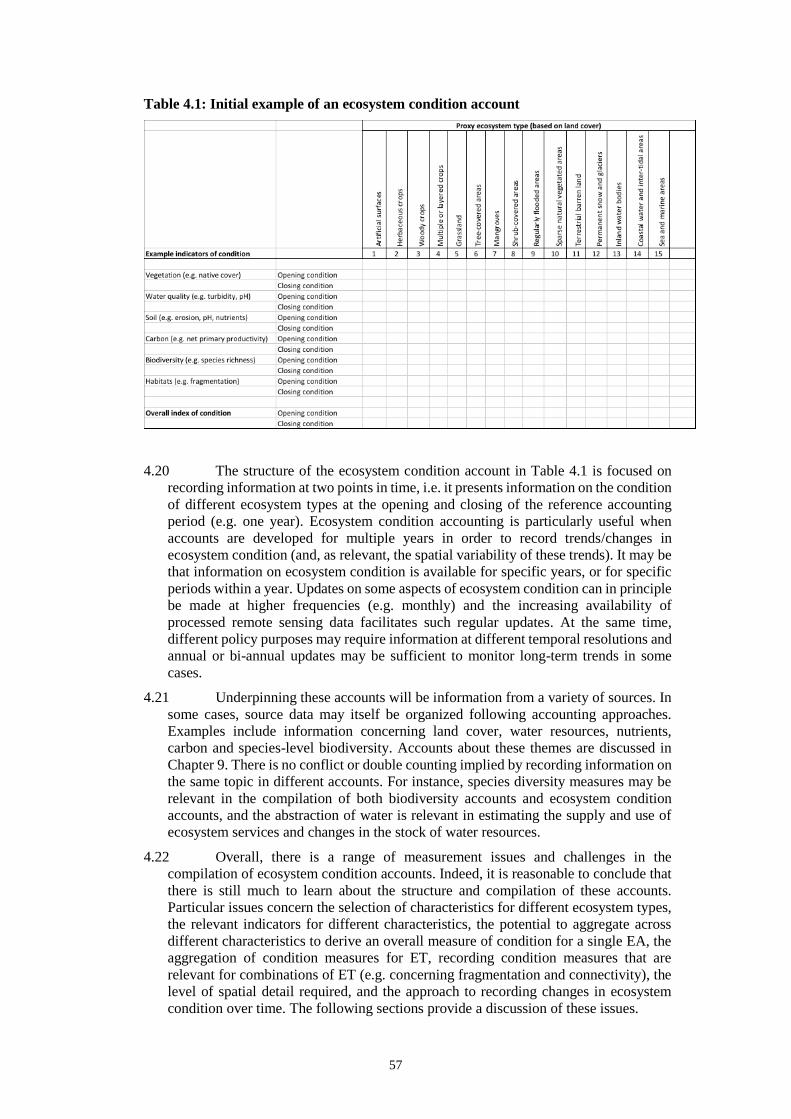
57

Table 4.1: Initial example of an ecosystem condition account

4.20 The structure of the ecosystem condition account in Table 4.1 is focused on

recording information at two points in time, i.e. it presents information on the condition

of different ecosystem types at the opening and closing of the reference accounting

period (e.g. one year). Ecosystem condition accounting is particularly useful when

accounts are developed for multiple years in order to record trends/changes in

ecosystem condition (and, as relevant, the spatial variability of these trends). It may be

that information on ecosystem condition is available for specific years, or for specific

periods within a year. Updates on some aspects of ecosystem condition can in principle

be made at higher frequencies (e.g. monthly) and the increasing availability of

processed remote sensing data facilitates such regular updates. At the same time,

different policy purposes may require information at different temporal resolutions and

annual or bi-annual updates may be sufficient to monitor long-term trends in some

cases.

4.21 Underpinning these accounts will be information from a variety of sources. In

some cases, source data may itself be organized following accounting approaches.

Examples include information concerning land cover, water resources, nutrients,

carbon and species-level biodiversity. Accounts about these themes are discussed in

Chapter 9. There is no conflict or double counting implied by recording information on

the same topic in different accounts. For instance, species diversity measures may be

relevant in the compilation of both biodiversity accounts and ecosystem condition

accounts, and the abstraction of water is relevant in estimating the supply and use of

ecosystem services and changes in the stock of water resources.

4.22 Overall, there is a range of measurement issues and challenges in the

compilation of ecosystem condition accounts. Indeed, it is reasonable to conclude that

there is still much to learn about the structure and compilation of these accounts.

Particular issues concern the selection of characteristics for different ecosystem types,

the relevant indicators for different characteristics, the potential to aggregate across

different characteristics to derive an overall measure of condition for a single EA, the

aggregation of condition measures for ET, recording condition measures that are

relevant for combinations of ET (e.g. concerning fragmentation and connectivity), the

level of spatial detail required, and the approach to recording changes in ecosystem

condition over time. The following sections provide a discussion of these issues.

58

4.4 Developing indicators of individual ecosystem characteristics

4.4.1 Selecting indicators

4.23 The SEEA EEA describes a number of different characteristics and associated

indicators (see for example Table 2.3 in the SEEA EEA). The development of

indicators to assess condition for particular purposes for particular ecosystem types, is

a relatively well-developed area of research. Bordt (2015a) provides a thorough

assessment of the indicators in the SEEA EEA and also describes a number of other

specific indicators that may be considered.

4.24 For a given characteristic, often the research enables the relative importance of

the different factors to be weighted to provide an appropriate composite index. The

challenge is not whether indicators of specific characteristics of ecosystem condition

can be measured, but rather which characteristics are relevant and how the indicators

might be combined.

4.25 If a fully spatial approach to ecosystem condition accounting is adopted, then

ideally, information on each selected characteristic would be measured or downscaled

to the BSU level. In many cases this may be possible and indeed, for some ecosystem

characteristics, such as those pertaining to soil retention and water flows, there may be

significant spatial variability that should be considered.

4.26 However, there will be some situations in which downscaling may make little

conceptual sense or imply assumptions in downscaling that are not appropriate. For

example, in measuring ecosystem condition for the purpose of providing habitats,

measures of fragmentation and connectivity are likely to be highly relevant. These

characteristics are conceptualised and measureable at a multiple ecosystem asset level.

Attribution of information on fragmentation and connectivity to the BSU level may be

possible, but the information remains meaningful only at broader scales. Further

investigation of the effects of scale on the measurement of condition for ecosystem

accounting is required.

4.27 One type of indicator not mentioned in SEEA EEA but which should be given

further consideration are functional indicators, for example of ecosystem resilience and

integrity. This may include, for instance indicators of physical or biological ecosystem

properties that reflect an ecosystem’s resilience for extreme events (see Carpenter et

al., 2010 for an overview). To the extent that scientific research has established a

functional indicator that relates well to the concept of ecosystem resilience, then such

indicators may be used directly for particular ecosystem types or may provide an

indication of the characteristics that should be the focus of condition measurement.

4.28 For example, even though a large number of indicators for coral reef condition

have been used in various monitoring and research programs, the indicator ‘percentage

live coral reef’ is considered a good aggregate indicator for coral reef condition. Even

though for site specific coral reef management other types of information may be

needed, this indicator may therefore be useful to express overall trends in reef condition

for an EA or ET. Where appropriate and where data are available this indicator could

be supplemented with a limited number of other condition indicators for instance

reflecting the presence or abundance of fish or other species indicative of habitat

quality, ecosystem functioning or correlated to ecosystem services (e.g. fisheries or

recreation).

4.29 However, generally, given data limitations, as well as from a conceptual

perspective, individual functional indicators are unlikely to be broadly applicable to

the variety of ETs within scope of ecosystem accounting. Instead, it is more likely that

59

ecosystem condition accounts can provide an organising structure for information

relevant to the derivation of functional indicators for different ETs within a country.

4.30 It is not expected that the measurement of condition for each ecosystem type

would require the use of a vast number of characteristics. From an ecosystem

accounting perspective, the intention remains to provide a broad indication of the level

and change in condition rather than to fully map the functioning of every ecosystem

asset. In this regard, a key element of accounting is monitoring change over time and

hence a focus on those characteristics that reflect changes in ecosystem condition is an

important consideration. Based on assessments of the various projects referred to

above, it seems that for most ecosystem types a set of 4-8 indicators can provide a

sound/robust set of information to enable assessment of the overall condition of an

ecosystem asset.

4.31 Five considerations that should be used in selecting indicators are (i) the degree

to which the indicator reflects the overall ecological condition of the ecosystem or key

processes within it and is able to signal changes in this condition; (ii) the degree to

which the indicator can be linked to measures of potential ecosystem services supply

(iii) how easy it is for policy makers and the general public to understand and correctly

interpret the indicator; (iv) data availability and scientific validity of measurement

approaches for the indicator; and (v) the possibility to generate new data cost

effectively. Note also that ecosystem condition will, in general, be more strongly linked

to potential ecosystem services supply than to actual ecosystem services supply since

the latter depends on the extent of use of the ecosystem by people.

4.32 To demonstrate the potential in this area, Box 4.1 shows tables for indicators

of ecosystem condition for different ecosystem types based on research in South Africa.

4.33 In terms of data sources, these will vary depending on the indicator selected.

In the areas of monitoring carbon, water and species-level biodiversity, a range of

potential data sources is introduced in Chapter 7. The ENCA QSP (Weber, 2014a) also

proposes many data sources in these areas. In many cases, satellite based data are likely

to be useful information especially in providing the breadth of data across different

ecosystem assets that is required for ecosystem accounting purposes.

4.34 Compilers are encouraged to consider the work described in the project

research papers, the outcomes from testing in different projects, and most importantly,

to engage with national experts on ecosystems and biodiversity measurement noting

that there may be different experts for different ecosystem types. A particular

ecosystem type to commence testing may be forests given their importance in many

countries and the significant literature on the measurement of forest characteristics (e.g.

dominant species, density and canopy cover, biomass and carbon stock).

4.35 Another starting point may be discussions with experts involved in national

reporting on the state and trends in biodiversity with the framework of the Convention

on Biological Diversity (CBD). Other international programs on ecosystem monitoring

and measurement will also be relevant including for example the collection of

information to monitor the UN Sustainable Development Goals and data collected

through the GEOSS program (e.g. within the Earth Observation for Ecosystem

Accounting (EO4EA) initiative.21 Within Europe, projects such as MAES, the EU

Habitat Directive and Copernicus will provide relevant information. Overall, the

ecosystem condition account is likely to be the primary account through which

engagement with the ecological community can be fostered.

21 https://www.earthobservations.org/activity.php?id=111

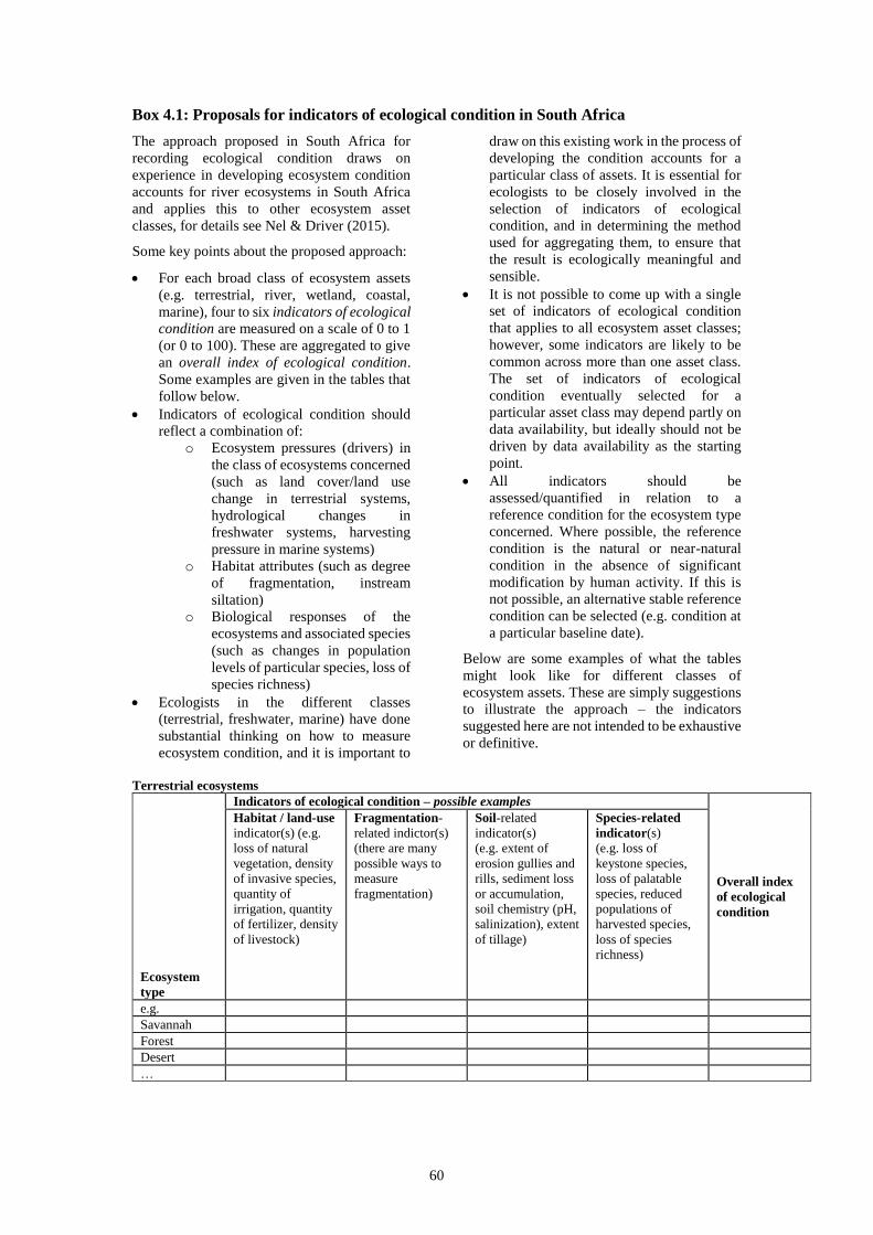
60

Box 4.1: Proposals for indicators of ecological condition in South Africa

The approach proposed in South Africa for

recording ecological condition draws on

experience in developing ecosystem condition

accounts for river ecosystems in South Africa

and applies this to other ecosystem asset

classes, for details see Nel & Driver (2015).

Some key points about the proposed approach:

• For each broad class of ecosystem assets

(e.g. terrestrial, river, wetland, coastal,

marine), four to six indicators of ecological

condition are measured on a scale of 0 to 1

(or 0 to 100). These are aggregated to give

an overall index of ecological condition.

Some examples are given in the tables that

follow below.

• Indicators of ecological condition should

reflect a combination of:

o Ecosystem pressures (drivers) in

the class of ecosystems concerned

(such as land cover/land use

change in terrestrial systems,

hydrological changes in

freshwater systems, harvesting

pressure in marine systems)

o Habitat attributes (such as degree

of fragmentation, instream

siltation)

o Biological responses of the

ecosystems and associated species

(such as changes in population

levels of particular species, loss of

species richness)

• Ecologists in the different classes

(terrestrial, freshwater, marine) have done

substantial thinking on how to measure

ecosystem condition, and it is important to

draw on this existing work in the process of

developing the condition accounts for a

particular class of assets. It is essential for

ecologists to be closely involved in the

selection of indicators of ecological

condition, and in determining the method

used for aggregating them, to ensure that

the result is ecologically meaningful and

sensible.

• It is not possible to come up with a single

set of indicators of ecological condition

that applies to all ecosystem asset classes;

however, some indicators are likely to be

common across more than one asset class.

The set of indicators of ecological

condition eventually selected for a

particular asset class may depend partly on

data availability, but ideally should not be

driven by data availability as the starting

point.

• All indicators should be

assessed/quantified in relation to a

reference condition for the ecosystem type

concerned. Where possible, the reference

condition is the natural or near-natural

condition in the absence of significant

modification by human activity. If this is

not possible, an alternative stable reference

condition can be selected (e.g. condition at

a particular baseline date).

Below are some examples of what the tables

might look like for different classes of

ecosystem assets. These are simply suggestions

to illustrate the approach – the indicators

suggested here are not intended to be exhaustive

or definitive.

Terrestrial ecosystems

Ecosystem

type

Indicators of ecological condition – possible examples

Overall index

of ecological

condition

Habitat / land-use

indicator(s) (e.g.

loss of natural

vegetation, density

of invasive species,

quantity of

irrigation, quantity

of fertilizer, density

of livestock)

Fragmentation-

related indictor(s)

(there are many

possible ways to

measure

fragmentation)

Soil-related

indicator(s)

(e.g. extent of

erosion gullies and

rills, sediment loss

or accumulation,

soil chemistry (pH,

salinization), extent

of tillage)

Species-related

indicator(s)

(e.g. loss of

keystone species,

loss of palatable

species, reduced

populations of

harvested species,

loss of species

richness)

e.g.

Savannah

Forest

Desert

…

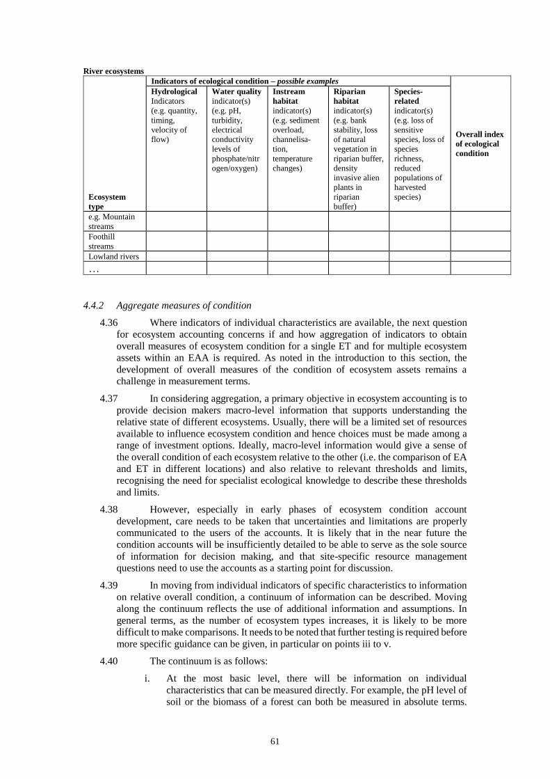
61

River ecosystems

Ecosystem

type

Indicators of ecological condition – possible examples

Overall index

of ecological

condition

Hydrological

Indicators

(e.g. quantity,

timing,

velocity of

flow)

Water quality

indicator(s)

(e.g. pH,

turbidity,

electrical

conductivity

levels of

phosphate/nitr

ogen/oxygen)

Instream

habitat

indicator(s)

(e.g. sediment

overload,

channelisa-

tion,

temperature

changes)

Riparian

habitat

indicator(s)

(e.g. bank

stability, loss

of natural

vegetation in

riparian buffer,

density

invasive alien

plants in

riparian

buffer)

Species-

related

indicator(s)

(e.g. loss of

sensitive

species, loss of

species

richness,

reduced

populations of

harvested

species)

e.g. Mountain

streams

Foothill

streams

Lowland rivers

…

4.4.2 Aggregate measures of condition

4.36 Where indicators of individual characteristics are available, the next question

for ecosystem accounting concerns if and how aggregation of indicators to obtain

overall measures of ecosystem condition for a single ET and for multiple ecosystem

assets within an EAA is required. As noted in the introduction to this section, the

development of overall measures of the condition of ecosystem assets remains a

challenge in measurement terms.

4.37 In considering aggregation, a primary objective in ecosystem accounting is to

provide decision makers macro-level information that supports understanding the

relative state of different ecosystems. Usually, there will be a limited set of resources

available to influence ecosystem condition and hence choices must be made among a

range of investment options. Ideally, macro-level information would give a sense of

the overall condition of each ecosystem relative to the other (i.e. the comparison of EA

and ET in different locations) and also relative to relevant thresholds and limits,

recognising the need for specialist ecological knowledge to describe these thresholds

and limits.

4.38 However, especially in early phases of ecosystem condition account

development, care needs to be taken that uncertainties and limitations are properly

communicated to the users of the accounts. It is likely that in the near future the

condition accounts will be insufficiently detailed to be able to serve as the sole source

of information for decision making, and that site-specific resource management

questions need to use the accounts as a starting point for discussion.

4.39 In moving from individual indicators of specific characteristics to information

on relative overall condition, a continuum of information can be described. Moving

along the continuum reflects the use of additional information and assumptions. In

general terms, as the number of ecosystem types increases, it is likely to be more

difficult to make comparisons. It needs to be noted that further testing is required before

more specific guidance can be given, in particular on points iii to v.

4.40 The continuum is as follows:

i. At the most basic level, there will be information on individual

characteristics that can be measured directly. For example, the pH level of

soil or the biomass of a forest can both be measured in absolute terms.

62

Looking at these measures over time can provide information on the

ecosystem’s condition.

ii. For some characteristics, it may be necessary to compare the chosen metric

with a known baseline, standard, threshold or limit, to be able to infer

something about ecosystem condition. For example, measures of water or

air quality will rely on both direct measures of pollutants and an

understanding of how the observed measure compares to a relevant

standard.

iii. At the third level, still for a single characteristic, a composite indicator

could be formed whereby a number of indicators are weighted together.

For such a composite indicator to be meaningful, it is necessary that the

component indicators are measured or interpreted in relation to a common

baseline or standard. Note that for many characteristics, for specific

ecosystem types, measurements at these first three levels are well

developed in the literature.

iv. At the fourth level, the aim is to consider, for a specific ET, some

combination of indicators, where each indicator relates to a different

characteristic. Two issues arise, first the selection of characteristics, and

second the means of combination. The first issue has been discussed in the

previous section. The solution to the second issue, as proposed in the

SEEA EEA, is the use of a reference condition, whereby indicators for

each characteristic are compared to the same reference condition for that

ecosystem.

v. At the final level, assuming that measures of ecosystem condition can be

established for each ET (i.e. at level four), it is necessary to find a means

of comparing across different ecosystem types. Again, the use of reference

conditions is a possible way forward where, in this case, all ET are

compared to a single reference condition. Selecting a reference condition

applicable to all ecosystems in a country, however, is a major challenge

both from a conceptual and from a data perspective. One potential option

is to select a specific year in order to define reference condition, however

any selected year will to be arbitrary to some extent. A further extension

at this level would be comparisons between countries.

4.41 Given the desire in accounting for macro-level information, it is the challenges

in measurement and interpretation at the last two levels that is of particular interest. A

focus is thus on the extent to which singular reference conditions can be used to either

compare within ETs, and/or to compare across ETs. This is discussed further in section

4.4.3 immediately below.

4.42 Assuming that an appropriate reference condition can be determined, the next

step is to normalise each indicator. This is commonly done by setting the reference

condition to a “score” of 100 and recording the actual condition as a score between 0

and 100. A related approach is to grade ecosystems on a scale of A – F (or similar),

with A representing the reference condition and F representing a condition most distant

from the reference.

4.43 Establishing reference conditions and normalising scores is another task that

should be conducted in close consultation with national experts in ecosystems and

biodiversity. Indeed, it may well be the case that there are existing bodies of work in

government agencies, research bodies and universities that can be used or built upon

to support this type of assessment. The use of reference conditions is well known in the

ecological literature and it should be considered for adaptation to ecosystem

accounting.

63

4.44 While the use of reference conditions is well known and practiced, the precise

choice of a reference or benchmark condition for accounting purposes requires further

discussion and testing. SEEA EEA notes a number of conceptual considerations with

respect to the use of reference condition approaches and Bordt (2015a) provides a more

complete consideration of different reference condition approaches. A short summary

of the issues is provided in the following sub-section.

4.45 Finally, following the logic outlined earlier in this section, even where each

indicator can be compared to an agreed reference condition, there remains the second

step of weighting together indicators of the different characteristics. The ambition is

not new from a statistical perspective (consider for example the Human Development

Index (UNDP, 2014)). However, as for socio-economic indicators, the weighting of

different ecosystem condition indicators is a matter of debate.

4.46 By far the easiest solution is to give each indicator equal weight in an overall

measure. However, this may not be appropriate from an ecological perspective with

different characteristics possibly playing a relatively more important role. Also, equal

weighting may not reflect the relative importance of different characteristics in the

potential supply of ecosystem services, or take into account various thresholds and non-

linearities which may apply in aggregating indicators that relate to different aspects of

condition.

4.47 An extended discussion on aggregation of ecosystem measures is provided in

Bordt (2015b). That paper points to a number of options and issues. At this stage, no

clear pathways forward have emerged but there are a number of areas for testing and

research described below in section 4.5.

4.4.3 Determining a reference condition

4.48 As noted above, determining an appropriate reference condition is not

straightforward and can be the matter of considerable debate. The discussion here

provides a short summary of the key points from an ecosystem accounting perspective.

4.49 A common starting point for determining a reference condition is application

of the idea of close-to natural or pristine condition where the reference condition

reflects the condition of the ecosystem asset if it had been relatively unaffected by

human activity. In many cases the application of this reference condition is done by

selecting a point in time at a pre-industrial stage. In Australia, for example, the year

1750 is commonly used.

4.50 A positive feature of this approach is that it places all ecosystem assets on a

common footing and “distance from natural” can be interpreted relatively equivalently

irrespective of the type of ecosystem. That is, it is possible to compare ecosystems that

are either extremely diverse, such as rainforests, or much less diverse such as deserts.

4.51 Unfortunately, what constitutes a natural ecosystem can lead to significant

debate particularly in those countries where human influence on the landscape has been

evident for thousands of years. For example, almost all of Europe may be considered

to have been forested at one point in time, but the use of this as a reference condition

for the current mix of ecosystem types is likely inappropriate because most of Europe’s

landscapes have been modified by people for several thousands of years. Many of

Europe’s fauna and flora species have had time to adjust to the management of these

landscapes by people and would not necessarily benefit from conversion to full forest

cover. In addition, the specific composition of the forest under natural conditions has

changed considerably in the last millennia and the choice of the specific forest to

represent natural conditions would always be arbitrary.

64

4.52 Another concern about the use of natural reference conditions for ecosystem

accounting is that they will not take into account the current use of the ecosystem. Thus,

to the extent that the focus of condition measurement is on the potential to supply

ecosystem services then assessment of condition in terms of “distance from natural”

will not compare like with like. This links directly to the earlier discussion on the use

of ecological and non-ecological factors in the assessment of condition. As this

discussion progresses the link to defining an appropriate reference condition must also

be made.

4.53 A related concern that arises is that the reference condition can be mistakenly

interpreted as a target or optimal condition. A clear distinction should be made between

reference and target conditions. A reference condition should be used solely as a means

of estimating relative condition and comparing across ecosystem characteristics and

ecosystem types. Target conditions, on the other hand, should be developed through

participatory processes, taking into account economic, social and environmental

considerations. For example, in urban areas the actual condition would be likely very

low or zero relative to a reference condition of the previous natural state of that area.

Hence, it would be inappropriate to suggest that the target condition should be the

natural state. A more appropriate target condition in urban areas might be the planting

of additional trees to contribute to improved air quality. Generally, it would be expected

that information on the actual and reference condition presented in ecosystem accounts

would be useful input to a discussion of target conditions.

4.54 For accounting purposes, it may be sufficient to use the condition at the

beginning of the accounting period as a reference condition and measure the actual

condition relative to that point in time. A variation on this approach is to select the

condition at the point in time at which the accounts commence.

4.55 The difficulty with this approach is that ecosystems that may have been heavily

degraded in the past will be compared from the same starting point as those that have

not been degraded at all – i.e. both would be given a reference condition of 100 at the

selected point in time.

4.56 On balance then, some degree of discretion is required in the selection of a

reference condition as well as transparency in methods and assumptions. In making a

decision, an important consideration is the scale of analysis. In general, it will be more

challenging to determine a reference condition as the scale of analysis gets larger since

there are more factors to take into account. Thus, if the intent is to only measure the

condition of a specific characteristic (e.g. soil condition) of a specific ecosystem type

(e.g. open grasslands), then the choice of reference condition may be made taking only

that characteristic and ecosystem type into account.

4.57 However, where there is a desire to compare multiple characteristics and

multiple ecosystems, then a relevant single reference condition will not be readily

apparent. For some countries, it may be that a pre-industrial time point gives an

appropriate reference condition, since there is a point in the not too distant past where

a relative common understanding of change from a reference condition can be

understood. As noted though, such a choice will likely not be appropriate where the

current landscape mix of ecosystem types has, to varying degrees, been evident for

centuries and a pre-industrial reference condition will only reflect ecological

characteristics.

4.58 Assuming a national level reference condition can be determined, a remaining

challenge is to find a reference condition that allows comparison across countries.

Given the diversity of landscape development patterns this choice is not at all obvious.

4.59 Pending further testing of different approaches to defining reference

conditions, it is recommended that in the development of ecosystem condition accounts

65

for a given country, that a point in time be selected, as far in the past as possible given

the availability of data, to allow the development of the relevant metrics of current

condition and the application of the reference condition approach. This is a pragmatic

starting point, particularly for the measurement of change over time within a country

and can support a focus on the direction and strength of trends in condition. It should

also help focus discussion on the challenging measurement issue of actually selecting

the indicators and maintaining ongoing time series. Using a relatively distant reference

point, rather than the beginning of the accounting period, will better support the

assessment of distance from thresholds for ecosystem assets.

4.60 To allow for comparison across countries, it will be necessary to move towards

common structures for the organisation and presentation of data on ecosystem

condition. Testing options for common structures that are both meaningful for

comparison purposes and also feasible for implementation is important. Another point

for testing is the potential for a country to use one reference condition domestically,

but to use a different reference condition for international comparison.

4.5 Recommendations for compiling ecosystem condition accounts

4.61 The measurement of ecosystem condition following the concepts in the

ecosystem accounting model is a complex task due the need to consider multiple

ecosystems and multiple characteristics. At the same time, there is sufficient research

in the general area of condition measurement to suggest that the testing of different

approaches in ecosystem accounting projects is quite possible and should be pursued.

4.62 An initial question in taking this work forward is how spatially variable

indicators can be aggregated both within and between ecosystems. For instance, soil

nutrient concentration may be highly relevant as an indicator of soil fertility and

thereby ecosystem condition, and have important repercussions for potential ecosystem

services supply, but aggregating this indicator is difficult. The average soil nutrient

concentration is meaningless since this may theoretically include 50% of the area with

very little soil nutrients and 50% of the area with excess nutrients. Therefore,

classifications (e.g. of soil fertility class) or comparison with reference conditions (e.g.

deviation from not degraded nutrient content) may be required.

4.63 Approaches to aggregate over space, over time and over ecosystem types will

depend upon policy questions, data availability and the required accuracy of the

condition account. It is recommended that the account be developed step-wise, by first

setting up the account for specific ETs and using a selected set of indicators. Over time

the accounts can be broadened in scope and filled with a larger range of indicators.

4.64 Some general recommendations and steps for the measurement of condition

are listed below. In each of these steps, the indicator's scientific validity, the ease of

communication and the availability of data should be considered.

• Select the measurement approach, i.e. using a minimum, partial or fully spatial

approach, and select a specific ET for initial focus.

• Select condition indicators that represent the main ecological characteristics of

the ETs. These may cover characteristics such as vegetation, water, soil,

biomass, habitat and biodiversity. Where relevant, condition indicators related

to land, water and forests should be compiled following the accounting of the

SEEA Central Framework. (This links to the broader role of thematic accounts

as discussed in Chapter 9).

• Consider whether indicators reflecting ecosystem integrity could be included

(including for example indicators of fragmentation, resilience, naturalness, and

ecosystem diversity).

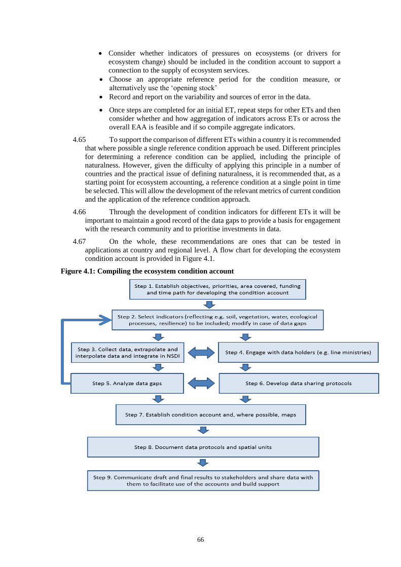
66

• Consider whether indicators of pressures on ecosystems (or drivers for

ecosystem change) should be included in the condition account to support a

connection to the supply of ecosystem services.

• Choose an appropriate reference period for the condition measure, or

alternatively use the ‘opening stock’

• Record and report on the variability and sources of error in the data.

• Once steps are completed for an initial ET, repeat steps for other ETs and then

consider whether and how aggregation of indicators across ETs or across the

overall EAA is feasible and if so compile aggregate indicators.

4.65 To support the comparison of different ETs within a country it is recommended

that where possible a single reference condition approach be used. Different principles

for determining a reference condition can be applied, including the principle of

naturalness. However, given the difficulty of applying this principle in a number of

countries and the practical issue of defining naturalness, it is recommended that, as a

starting point for ecosystem accounting, a reference condition at a single point in time

be selected. This will allow the development of the relevant metrics of current condition

and the application of the reference condition approach.

4.66 Through the development of condition indicators for different ETs it will be

important to maintain a good record of the data gaps to provide a basis for engagement

with the research community and to prioritise investments in data.

4.67 On the whole, these recommendations are ones that can be tested in

applications at country and regional level. A flow chart for developing the ecosystem

condition account is provided in Figure 4.1.

Figure 4.1: Compiling the ecosystem condition account

67

4.6 Issues for research on ecosystem condition

4.68 At this stage in the development of ecosystem accounting, the most important

work required on ecosystem condition is the testing of the approach described in this

chapter and the comparison of experiences across ETs and countries. In undertaking

this testing there are, however, some specific research questions that should be

considered.

4.69 Most importantly, a clearer direction is needed on the extent to which the

characteristics used for the measurement of condition go beyond ecological

characteristics and also incorporate non-ecological characteristics, including for

example indicators of environmental pressures on ecosystems. This issue must be

considered so as to provide clarity on the way in which the concept of ecosystem

condition for ecosystem accounting purposes relates to the measurement of ecosystem

services and concepts of ecosystem capacity and ecosystem capability (as described in

Chapter 7).

4.70 Given these requirements for conceptual clarity, specific work is required to

identify condition indicators that facilitate connecting condition to the ecosystems’

potential and capacity to supply ecosystem services. This includes coming to a better

understanding of information gaps, i.e. between the data required to comprehensively

monitor ecosystem condition vis-a-vis naturalness and capacity and potential to supply

ecosystem services, and the data actually available from the various sources.

4.71 Further research is also required on the choice of reference condition for

ecosystem accounting purposes. For some regions in some countries, using natural

ecosystems as the reference condition may be appropriate. However, more generally it

will be necessary to establish non-natural reference conditions perhaps based on a

historical baseline or a condition prescribed in policies (e.g. on water quality), and also

taking into account links to the supply of ecosystem services.

4.72 Beyond a focus on measurement of condition for specific ET, there also

remains work to be done on defining and incorporating condition indicators applicable

at larger scales such as habitat fragmentation or ecosystem diversity. This work should

also be seen in a broader context of taking into account scale effects in the measurement

of ecosystem condition and ecosystem services.

4.73 A final area research is the development of overall indexes of condition for

ecosystem assets either based on aggregation of indicators for selected characteristics

or using some alternative approach, for example isolating a key characteristic in

ecological terms. A range of different approaches are available for aggregation, ranging

from using an equal weight for all indicators, to weighing based on expert judgement,

or weighing based on specific criteria, for instance in relation to indicators aggregated

by ecosystem compartment (soils, vegetation, etc.), by species group (e.g. weighting

of insects, mammals, plants, etc.) and/or taking into consideration key ecosystem

services.

68

5 Accounting for flows of ecosystem services

Key points in this chapter

In ecosystem accounting, ecosystem services are defined from the perspective of contributions that

ecosystems make to benefits used in economic and other human activity. It is therefore important to

distinguish clearly between ecosystem services and benefits.

Generally, most focus for national level accounting is on final ecosystem services. All final ecosystem

services have a direct link between ecosystems and economic units.

Intermediate ecosystem services are important for understanding relationships and dependencies

between ecosystem assets. They can be incorporated into the ecosystem accounting model but they are

not a priority area for measurement. Further discussion and research on accounting for intermediate

ecosystem services is required.

The use of a classification of ecosystem services, such as CICES, FEGS-CS or NESCS is an important

aspect in compiling estimates of ecosystem services flows.

There are two principal ways to populate the Ecosystem Services Supply and Use account with data. The

first approach starts with data that is already in the national accounts and identifies the ecosystem

contribution to the benefit involved. Preparation of maps subsequently requires spatial allocation of data

on ecosystem services.

The second approach is required for ecosystem services that are not connected to a specific benefit

measured in the accounts. This is often the case for regulating services. In this case spatial models or

direct measures are required to quantify the ecosystem services.

In order to construct the Ecosystem Services Supply and Use account it is necessary to consider the use

of ecosystem services by different economic units including households, businesses and governments.

In some cases, biodiversity may be considered a cultural ecosystem service but generally, biodiversity is

best considered as a characteristic of ecosystem assets that can be degraded or improved over time, and

which underpins the supply of ecosystem services. It is recorded in the thematic account for biodiversity

and as part of ecosystem condition accounts.

5.1 Introduction

5.1. Ecosystem services are the glue that enables the connection to be made

between ecosystem assets on the one hand and economic production and consumption

on the other. Their measurement is thus central to the aim of integrating environmental

information fully into the existing national accounts.

5.2. Since the release of the Millennium Ecosystem Assessment (MA) in 2005

(MA, 2005) there has been a strong increase in the number of studies on ecosystem

services. The studies have focused on many aspects of definition and measurement,

and have involved researchers from a range of disciplines. Subsequent work in the

context of the TEEB (The Economics of Ecosystems and Biodiversity) Study (TEEB,

2010a&b), the MAES initiative (Maes, et al., 2014) and the Inter-governmental

Platform on Biodiversity and Ecosystem Services (IPBES) have reinforced the

potential of the ecosystem services approach in understanding the relationship between

humans and the environment. Ecosystem accounting has built upon this work and

research. The SEEA EEA attempts to chart a course through the various discussions on

ecosystem services and it makes a range of choices about the definition and

measurement of ecosystem services for accounting purposes.

5.3. To support discussion in this chapter, the following paragraphs provide a brief

summary of the framing for ecosystem services in the SEEA EEA as presented in

Chapter 2. In ecosystem accounting, each ecosystem asset generates a set or basket of

final ecosystem services which are defined as contributions to the production of

69

benefits. Final ecosystem services encompass a wide range of services provided to

economic units (businesses, governments and households) and may be grouped into

provisioning services (i.e. those relating to the supply of food, fibre, fuel and water);

regulating services (i.e. those relating to actions of filtration, purification, regulation

and maintenance of air, water, soil, habitat and climate) and cultural services (i.e. those

relating to the activities of individuals in, or associated with, nature).

5.4. Benefits may be either SNA benefits - goods or services (products) produced

by economic units (e.g. food, water, clothing, shelter, recreation) currently included in

the economic production boundary of the SNA; or non-SNA benefits – benefits that

accrue to individuals, or society generally, that are not produced by economic units

(e.g. clean air). By convention, the measurement scope of non-SNA benefits for

ecosystem accounting purposes is limited to the flow of ecosystem services with an

identifiable link to human well-being.

5.5. In the accounting system, for each supply of final ecosystem services there is

a corresponding use that leads to the production of either an SNA or non-SNA benefit.

Further, in each sequence of use of ecosystem services and production of benefits there

is an associated user or beneficiary being an economic unit – business, government or

household. Thus, every final ecosystem service flow represents an exchange between

an ecosystem asset (as a producing/supplying unit in the accounting system) and an

economic unit.

5.6. Building on this framing of ecosystem services in ecosystem accounting, this

chapter summarises the main points from the SEEA EEA concerning ecosystem

services, discusses refinements to the SEEA EEA discussion, and describes the main

measurement issues and remaining challenges. Section 5.2 describes the ecosystem

service supply and use accounts and section 5.3 discusses issues in the definition of

ecosystem services. Section 5.4 considers approaches to the classification of ecosystem

services. Sections 5.5 and 5.6 summarize the role and use of biophysical modelling and

the relevant data sources, materials and methods for measuring ecosystem service

flows. Practical recommendations for compiling an ecosystem services supply and use

table are provided in section 5.7, including a flow chart and an example. Section 5.8

presents selected topics for research.

5.2 Ecosystem services supply and use accounts

5.2.1 Introduction

5.7. The ecosystem services supply and use account records the actual flows of

ecosystem services supplied by ecosystem types and used by economic units during an

accounting period. Ecosystem accounting generally, and the ecosystem supply and use

account in particular, focus on ecosystem services and the connections to the

production and consumption of other goods and services. The scope does not extend to

measuring the broader costs and benefits that may arise from increased or reduced

consumption such as health and social outcomes. Thus, ecosystem accounting does not

provide an economic or social welfare perspective on the relationship between people

and the environment. At the same time, information on the supply and use of ecosystem

services recorded in the accounts will support discussion of relevant welfare outcomes

(see further discussion in Chapter 6).

5.8. For accounting purposes, the concept of the supply of ecosystem services is

that supply is equal to the use or receipt of the services during an accounting period.

That is, supply is not recorded if there is no corresponding use. It may be quite relevant

to measure the potential or sustainable level of supply that could be delivered by an

ecosystem asset (the corresponding concepts of ecosystem capacity and potential

70

supply are further discussed in section 7.3). However, they are not the focus of

measurement in the supply and use accounts.

5.9. Recording supply as equal to use reflects that, from an accounting perspective,

ecosystem services are considered to reflect revealed transactions or exchanges that

take place between ecosystem assets on the one hand and economic units (businesses,

households, governments) on the other. It is implicitly assumed that each transaction is

distinct and hence each ecosystem service is separable.

5.10. The data in an ecosystem service supply and use account relate to a given EAA

and should be structured by type of ecosystem service (e.g. timber provision, water

purification). A supply and use account may be compiled in both physical and

monetary terms.

5.2.2 Overall structure of the supply and use accounts

5.11. The structure of the ecosystem services supply and use account is shown in

Table 5.1. The various quadrants, labelled A – H reflect the following information.

Note that the listing of ecosystem service types in the table is indicative only and, in

due course, should reflect an agreed classification of ecosystem services.

• A: No data are recorded in this quadrant as in concept economic units

cannot supply ecosystem services.

• B: In this quadrant, the supply of ecosystem services by ET is recorded.

• C: This quadrant is the equivalent of the standard physical supply and use

table showing the supply of products by different economic units. This

reflects the production of benefits to which the ecosystem services

contribute. The scope of products is all goods and services produced in an

economy. The economic units are broken down here by type of activity

and hence encompass both private and public sector production.

• D: No data are recorded here as, in concept, ecosystems cannot supply

products (i.e. goods and services within the SNA production boundary).

• E: Here the use of ecosystem services by type of economic unit is recorded.

This includes both the use of ecosystem services as input to further

production and the use of ecosystem services as final consumption.

• F: This quadrant provides an opportunity to record intermediate ecosystem

services, i.e. services supplied by EAs and used by other EAs. If these

flows were to be recorded then the supply of ecosystem services in

quadrant B would need to have an equivalently larger scope. (Further

discussion on intermediate services is in section 5.3.)

• G: This quadrant is the equivalent of the standard physical supply and use

table showing the use of products by different economic units.

• H: No data are recorded here as, in concept, ETs cannot use products.

5.12. The structure of the ecosystem services supply and use account incorporates

flows of products. This supports the joint presentation of data on both the ecosystem

services used by economic units, and the products (SNA benefits) to which those

ecosystem services contribute. In terms of the quadrants of Table 5.1, the output of

products such as livestock are recorded in the first column of quadrant C (under

agriculture) and the use of ecosystem services (e.g. grass consumed directly by

livestock) would be recorded in the same column in quadrant E. (The original supply

of those ecosystem services would be recorded in quadrant B.) As desired, quadrant G

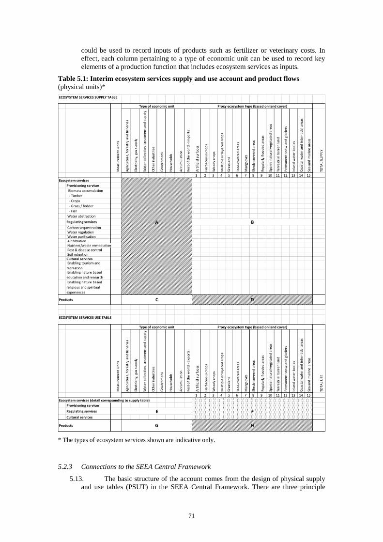
71

could be used to record inputs of products such as fertilizer or veterinary costs. In

effect, each column pertaining to a type of economic unit can be used to record key

elements of a production function that includes ecosystem services as inputs.

Table 5.1: Interim ecosystem services supply and use account and product flows

(physical units)*

* The types of ecosystem services shown are indicative only.

5.2.3 Connections to the SEEA Central Framework

5.13. The basic structure of the account comes from the design of physical supply

and use tables (PSUT) in the SEEA Central Framework. There are three principle

72

alterations. First, rather than showing just one column representing the environment,

there are multiple columns each representing an ET.

5.14. Second, in the SEEA Central Framework PSUT there are three types of flows

– natural inputs, products and residuals. In concept, ecosystem services align generally

to the concept of natural inputs but in the SEEA Central Framework the coverage is

limited to provisioning services and there may be differences in the descriptions of the

flows to be considered. Regulating and cultural services are excluded. It is noted that

some regulating services are related to flows of residuals (e.g. emissions, pollution,

waste) recorded in the SEEA Central Framework, for example, there will be a

connection between residual flows of air pollutants and air filtration services.

Conceptually, however these are different flows (see further discussion below).

5.15. Third, the ecosystem services supply and use account includes the potential to

record intermediate services. Since the SEEA Central Framework does not consider

the ways in which different environmental assets may be connected, i.e. it provides an

individual resource perspective, the recording of intermediate ecosystem services

reflecting the dependencies between ecosystem assets, is a unique feature of ecosystem

accounting.

5.16. In line with the SEEA Central Framework, ecosystem services are recorded

before deducting any natural resource residuals.22 Thus, for instance, in the case of

timber harvesting, the biomass that is felled reflects the quantity of the ecosystem

service in the same way as this is regarded as the flow of natural inputs in the SEEA

Central Framework. However, further work is needed on how to define and record

flows of natural resource residuals in an ecosystem accounting context.

5.2.4 Recording the connection to economic units

5.17. Economic units and ecosystem assets: In recording the supply of ecosystem

services, it is important to distinguish between economic units and ecosystem assets.

Following the ecosystem accounting framework described in Chapter 2, only

ecosystem assets can supply ecosystem services that are subsequently received by

economic units. For example, in the case of agriculture or forestry related ecosystem

services, although an economic unit (e.g. a farmer or forester) may manage the

associated ecosystem, for accounting purposes, in these instances, the farmer and

forester should be seen as using inputs from ecosystem assets (i.e. the ecosystem

services) to supply benefits (crops, timber, etc.) that are produced by combining

ecosystem services inputs with inputs from other economic units (fuel, fertiliser, etc.).

5.18. Although in the table the supply of ecosystem services is shown as only

emerging from ecosystem assets (quadrant B), there may be interest in attributing the

supply of services to particular economic units. For example, ecosystem services that

are inputs to cropping or livestock rearing activities could be considered to be supplied

by agricultural businesses that are managing the associated ecosystem asset. This

alternative presentation could be recorded in a stand-alone table following the rows and

column structures used for quadrant A in Table 5.1. This recording should be

reasonably straightforward for provisioning services. However, it may be more

difficult to attribute the supply of some of regulating and cultural services to specific

economic units.

5.19. Economic units, ecosystem services and residual flows: As noted above, the

SEEA Central Framework records flows of residuals (e.g. emissions, pollution, waste).

Residual flows are not ecosystem service flows but rather reflect physical flows from

22 Note these residual flows are additional to the residuals relating to emissions and the like mentioned above.

73

economic units into the environment. While these are conceptually different flows,

there are important relationships to consider. Specifically, several regulating services

involve the break-down or absorption of the substances present in residual flows. In

this context, these ecosystem services may be considered to provide “sink services”,

i.e. the ecosystem acts as a sink or receiver of residuals from economic activity.

5.20. From an accounting perspective, the extent of the ecosystem services is limited

in two ways. First, there must be a related demand for the service, i.e. there must be a

human use benefiting from the break-down or absorption of the residual substances.

For example, when rivers purify water from excess nutrients discharged by various

economic sectors, a service is only supplied if there is water abstraction for human use

downstream where the removal of nutrients provides a benefit (e.g. because of reduced

efforts required to clean the water through water treatment). Second, it may be the case

that not all of the quantity of residual flow is able to be broken-down or absorbed in

ecosystem processes. In this case, the level of the ecosystem service is limited to the

quantity of the substance that is absorbed and some quantity will remain unmediated.

These excess quantities may be of particular interest in the measurement of

environmental pressures as they relate to changes in ecosystem condition. Overall,

information concerning residuals is related to but different from ecosystem services

and hence entries for residual flows and ecosystem services should not be recorded in

a single table.

5.2.5 Compiling the ecosystem services supply table

5.21. A likely challenge in compiling the supply table will be attributing the supply

of ecosystem services to a specific EA and ET. This is unlikely to be an issue for

provisioning services, but it may be of concern for regulating services and some

cultural services in cases where the service is provided through a combination of

different EA within a landscape.

5.22. Given this, it is recommended that, as a first step in accounting for ecosystem

services, compilers create a table showing which ecosystem services are likely to be

supplied from different ET for their country or target ecosystem accounting area.23 In

undertaking this task, a classification of ecosystem services (such as CICES, FEGS-CS

or NESCS see section 5.4) can be used as a form of checklist.

5.23. It is to be expected that for some services, particularly regulating services such

as carbon sequestration, the same service will be supplied by more than one ET. Also

for some ecosystem services, the service will be supplied as a result of the combined

production of neighbouring ET.24 For example, cultural services supplied by a mix of

ETs (e.g. lakes and wetlands). In these cases, some allocation of ecosystem service

flow between ET will be required.

5.24. It will be relevant to use this initial table as a discussion document to obtain

input from various experts, including specialists in specific ecosystem types and/or

specific ecosystem services. It is also important that the development of such a table is

informed by people experienced in considering the link between ecosystems and

economic and human activity. This should ensure that commonly overlooked services,

particular various regulating services, are not ignored. This initial table would also

serve as a basis for scoping and prioritising the required work, and comparing

compilation exercises across countries (for example comparing lists of ecosystem

services attributed to grasslands).

23 To provide a starting point for this work consider the material in Bordt (2017). 24 Note that this is different from the notion of combined production where ecosystem services are combined

with human inputs (labour, energy, etc.) to produce benefits.

74

5.25. The proposed ecosystem services supply table (Table 5.1) has columns

reflecting the various ecosystem types and rows reflecting different ecosystem services,

in this case classified following CICES. In this table, there is no direct recording of the

users of ecosystem services, this takes place in the ecosystem services use table.

However, it will be important to compile information on the combination of ET,

ecosystem services and users at the same time.25

5.26. The choice of indicators for measuring the flows of different ecosystem

services is discussed in section 5.6 along with relevant data sources and examples.

5.27. The ecosystem services supply table shown in Table 5.1 can be compiled in

physical terms and in monetary terms. When compiled in physical terms each

ecosystem service will have a different measurement unit. One consequence of this is

that there can be no aggregation of different ecosystem services because the relative

importance of individual ecosystem services cannot be immediately determined.

Aggregation within a single row to estimate a total flow from all ETs for an individual

service is possible. Indeed, in practice, for some services, compilation may involve

using aggregate information (e.g. country level data) for an ecosystem service and then

allocating that information to ET and potentially to individual EA.

5.28. Compilation in monetary terms usually occurs by estimating values

corresponding to the physical flows of each ecosystem service, noting that direct

measurement of values may be possible for some provisioning services. The ecosystem

services supply table shown in Table 5.1 can then be extended with additional rows to

record the total flows of ecosystem services in monetary terms. The estimation of

values for ecosystem services is discussed in Chapter 6.

5.2.6 Compiling the ecosystem services use table

5.29. The difference between the supply and the use tables is that the focus of the

use table is on the link between ecosystem services and different types of users, while

the supply table focuses on the supply from ET. Users include economic units classified

by industry, government sector and household sector units, following the conventions

applied in the national accounts.

5.30. The focus on users arises because, while the supply of ecosystem services can

be directly linked to a spatial area (e.g. to an EA), there is no requirement that the

location of the user is the same as the location of the area from which the ecosystem

service is supplied. This is especially the case for regulating services but also for some

cultural services.

5.31. The link between users and the spatial areas from which ecosystem services

are supplied is often complex but its measurement is increasingly common (see Hein

et al., 2016). In framing the measurement in this area, it will be relevant to consider,

for different ecosystem services, whether the beneficiaries are, in general terms, local,

national or global. For example, in the case of most provisioning services, the users

will be located within the supplying EA, i.e. at the point of extraction or use (e.g.

farmers, foresters, fishermen, water supply companies). This will also be true of many

cultural services where there is a recreational or touristic component. That is, although

the beneficiary will likely reside away from the supplying EA, the ecosystem service

is consumed when the user is present in the EA (e.g. walking in a forest, swimming in

a lake). However, for many regulating services, the users will be located in

25 Note that the FEGS-CS and NESCS structures explicitly incorporate this connection between supply and

beneficiaries.

75

neighbouring ecosystems (for example, air filtration) or will be global users (for

example, with respect to carbon sequestration).

5.32. Given the lack of a singular spatial connection, the choice of structure of the

ecosystem services use table must be guided by possible uses and analysis of data. The

choice made in Table 5.1, is to structure the ecosystem services use table showing the

allocation of the total supply of each ecosystem service to the various economic units,

without distinguishing the precise location of the user. This allocation provides a

framing aligned to the structure of national accounts datasets.

5.33. As for the ecosystem services supply table, the use table may be compiled in

both physical and monetary terms. In physical terms, entries will be limited to

indicators for each ecosystem service. Since in accounting terms, supply must equal

use, the unit of measurement applied for each ecosystem service must be the same in

both the supply and use account in order for a balance to be obtained.

5.34. In monetary terms, entries for the total use of ecosystem services can be

derived both for individual ecosystem service types and for total use by each user. The

estimation of values for ecosystem services is discussed in Chapter 6.

5.35. The presentation of the tables outlined here may suggest that the supply of

ecosystem services would necessarily be compiled before measuring the use of

ecosystem services. In practice, the reverse may be the case and, in preference,

compilation of the supply and use estimates should take place concurrently. For

example, measures of provisioning services are likely to be estimated based on

measures of the extraction of materials (e.g. timber) from the environment by economic

units, i.e. a use perspective. Indeed, since for all final ecosystem services there must be

some link to economic units and other human activity, there is a strong case for

compiling both the supply and use of ecosystem services at the same time.

5.3 Issues in the definition of ecosystem services

5.3.1 Introduction

5.36. Because of the ambition to integrate measures of ecosystem services with the

standard national accounts, the measurement scope and definition of ecosystem

services in the SEEA EEA is defined in relation to the production boundary of the SNA.

The SNA boundary sets the scope for the measurement of GDP and related measures

of production, income and consumption. For ecosystem accounting, the production

boundary is expanded relative to the SNA reflecting that the supply of goods and

services by ecosystems is considered additional production.

5.37. An important part of the rationale for measuring ecosystem services is that

much economic production (for example in agriculture, forestry and fisheries) utilizes

inputs directly taken from ecosystems but these inputs (and any associated costs of

capital) are not recorded in the standard accounting framework. In these situations, the

logic of the SEEA EEA is that flows of ecosystem services should be clearly

differentiated from the goods and services that are produced. Thus, the ecosystem

services represent the contribution of ecosystem assets to the production of those goods

and services. In effect, this sets up an extended input-output or supply chain that

includes ecosystem assets as suppliers.

5.38. It is noted that the SNA production boundary currently includes goods and

services produced through illegal activity and subsistence production, i.e. these

products form a part of the set of SNA benefits. The expansion in scope of the

production boundary in the SEEA EEA will mean that ecosystem services that provide

input to the production of these goods and services will also be recorded. Data and

76

methods for measurement in these areas are discussed in Handbook on measurement

of the non-observed economy (OECD et al., 2002).

5.39. A second important part of the rationale for measuring ecosystem services is

the understanding that there are many other, non-SNA, benefits that economic units,

and society more generally, receive from ecosystem assets. Hence, a full and proper

accounting should incorporate this production of services by ecosystems, and the

consumption of them in economic and human activity.

5.40. While this provides a clear rationale the remainder of this section discusses

factors that need to be taken into consideration to ensure a clear measurement boundary

is established.

5.3.2 Distinguishing ecosystem services and benefits

5.41. The SEEA EEA accounting model makes a clear distinction between

ecosystem services and the benefits to which they contribute. From an accounting

perspective, the distinction is meaningful since:

• it allows description of the relationship between final ecosystem service flows and

existing flows of products (SNA-benefits) currently recorded in the SNA

• it recognizes the role of human inputs in the production process and that the

contribution of final ecosystem services to benefits may change over time (e.g.

due to changes in the methods of production)

• it helps in identifying the appropriate target of valuation since the final ecosystem

services that contribute to marketed products (e.g. crops, timber, fish, tourism

services) will only represent a portion of the overall value of the corresponding

benefits.

5.42. For these reasons, the principle of distinguishing between final ecosystem

services and benefits is appropriate for ecosystem accounting. It is also consistent with

the approach taken in TEEB (2010a), Banzhaf and Boyd (2012) and the UK NEA

(2011), although the precise boundaries, definitions and terms applied for

distinguishing between final ecosystem services and benefits vary in the different

cases.

5.43. In practice, particularly at large scales, the explanation and application of this

distinction can be challenging. The issues arise differently for provisioning services,

regulating services and cultural services. For provisioning services, the main challenge

is effectively describing the various ecosystem services involved in supplying

cultivated biological resources26. These outputs, including crops, plantation timber, and

aquaculture, are considered benefits produced as a combination of final ecosystem

services and human inputs. Since the balance of inputs between final ecosystem

services and human inputs will vary by production process (e.g. between hydroponic,

irrigated and rainfed agriculture), it means that using a measure of output from

production as a measure of the quantity of ecosystem service will be misleading.

5.44. For regulating services, there are generally no direct human inputs consumed

in the production of benefits (although there may be economic activity associated with

managing or altering an ecosystem to support the generation of such services, e.g. in

establishing vegetation as part of a carbon capture program). However, note that the

description of the service and the benefit will be different. Thus, the description of the

service will reflect the action of the ecosystem asset – sequestering carbon or capturing

26 Cultivated biological resources is a term from the SNA that supports the distinction between biological

resources (e.g. timber, fish, animals, etc.) the growth of which is considered the output of a process of

production – i.e. cultivated; and those whose growth is the result of natural processes – i.e. natural biological

resources.

77

air-borne pollutants, while the benefits should be described in terms of increased

stability of climate and cleaner air. Making this distinction is important to ensure the

correct focus for measurement and valuation. Changes in the volume of cleaner air, for

example, may be caused by the presence of air filtration services or from reductions in

vehicle emissions. Only the former should be the focus of measurement for ecosystem

accounting. Note that although there may be costs incurred in establishing or

maintaining an ecosystem to support the supply of regulating services, these are not

considered direct inputs to the generation of ecosystem services.

5.45. For cultural services, the contribution of ecosystems is relatively passive in

that it is commonly the ecosystem providing opportunities for people to engage in

activities, learning experiences and the like. Costs may be incurred to facilitate people

benefiting from these services, such as the construction of cycling or hiking paths,

visitor facilities, etc. Often, cultural services are conceptualised in terms of the benefits

that people receive from the engagement with ecosystems. The challenge for ecosystem

accounting is to estimate the contribution of the ecosystem itself to the generation of

benefits.

5.46. The challenge is to appropriately describe the ecosystem service such that the

focus of measurement is appropriate. The focus in describing the ecosystem service

should be a description of ecosystem processes that reflect the contribution of the

ecosystem to the production of the benefit – i.e. what is the ecosystem doing? Overall,

much further discussion on the framing and descriptions of ecosystem services and

corresponding benefits will be required to ensure a common understanding of

measurement in this area.

5.47. Note that in some cases these challenges are larger where it concerns the

physical measurement of ecosystem services, compared to the measurement of services

in monetary terms. For example, in the case of timber plantations, the (SNA-) benefit

is represented by the accumulation of wood in the plantation in a given time period,

usually a year. The service is comprised of the various ecological processes that

underpin the accumulation of wood, such as storing and releasing nitrogen and

phosphorus to the trees. In physical terms these services are difficult to quantify and

aggregate, and in practice the accumulation of timber (in m3) may need to be taken as

indicator for both the service and the benefit. In monetary terms, the benefit is

represented by the value of the produced volume of timber. The service, on the other

hand, can be valued using a residual approach (i.e. by calculating a resource rent) in

order to specify the value of the contribution of natural capital involved in producing

the benefit (see for further detail section 5.4).

5.3.3 Distinguishing final and intermediate ecosystem services

5.48. All ecosystem services, final and intermediate, should be considered in relation

to ecosystem processes and ecosystem characteristics within ecosystem assets. A focus

only on final services serves to recognise the important role that these processes and

characteristics play in directly supporting economic and human activity. Recognising

that intermediate services can also be recorded in the accounting framework supports

a better conceptualisation of the connections and dependencies between ecosystem

assets. This illustrates the potential of ecosystem accounting to recognise the

contributions of all ecosystems and associated ecosystem processes wherever they are

located and to understand the potential impacts of economic production and

consumption on ecosystem assets.

5.49. While it is relatively straightforward using accounting principles to distinguish

between final and intermediate ecosystem services, the complexity of ecosystems

means that it can be difficult to make this distinction in practice. At an aggregate level,

78

a focus on only final ecosystem services may be sufficient since many intermediate

services will reflect services supplied to other ecosystem assets within the same EAA.

However, this may not be appropriate when considering the contribution of individual

ecosystems or when undertaking accounting for smaller areas or individual ETs. In

these cases, it may be quite relevant to understand the contribution of discrete EAs or

ETs especially if an important function of an ecosystem asset is to support

neighbouring ecosystem assets.

5.50. A typical example would be the intermediate services provided by upstream

forests in regulating water flows and limiting sediment content in water that is

subsequently abstracted downstream (at which point final ecosystem services would be

recorded). In this case it may be relevant to record the generation of ecosystem services

by the forest ecosystem asset, the use of these services by the downstream water

ecosystem asset (i.e. the river), and the generation of final ecosystem services by the

water ecosystem asset at the point of abstraction.

5.51. Another example concerns pollination. Pollination in croplands may depend

upon pollinators that require shrublands or forest habitat, for instance for shelter. If the

shrublands or forests would be converted, the pollination service to the croplands

would be diminished or lost. In this case, adding pollination services and the biomass

accumulation of crops would lead to double counting. Thus, it will be relevant to map

and record such intermediate services because otherwise the services provided by

different ecosystem types such as forests and shrublands may be underestimated, for

instance in spatial planning.

5.52. The use of the term intermediate services may cause some confusion. The

following points are relevant in the use of this term in the Technical Recommendations.

i. The use of the term intermediate in this context is analogous to the use of

the term in the SNA with respect to flows of goods and services between

producing economic units, i.e. intermediate consumption. In ecosystem

accounting, intermediate services are supplied by one EA to another EA.

ii. In some circumstances, there may be interest to record flows of services

that are internal to an ecosystem asset (just as there may be with flows

within an economic unit). These can be recorded as required for analytical

purposes but from a supply and use perspective the net position will be

zero for a single ecosystem asset.

iii. When considered from an integrated economic-ecosystem perspective,

final ecosystem services could be considered to be intermediate to the

extent that the ecosystem services are inputs to SNA benefits (currently

recorded goods and services). However, the term final ecosystem services

is retained due to its common usage and to reflect that these services are

final with respect to an ecosystem-only perspective.

iv. In the SEEA EEA, intermediate services were aligned with physical flows

between and within ecosystem assets – i.e. inter- and intra- ecosystem

flows. These physical flows can be recorded (e.g. of water, nutrients,

pollen) and they may be important for some analytical and policy needs.

Information on these flows may also be relevant in the estimation of

intermediate services but they are conceptually different flows. By way of

example, the retention of sediment by upstream forests is a service

provided to downstream ecosystem assets but the flow of the service is, in

fact, evidenced by the lack of a physical flow of sediment.

5.53. Notwithstanding the accounting possibilities with respect to intermediate

services and that recording these flows may help in better understanding flows of final

ecosystem services and the contribution of different ETs, it is not advisable to attempt

79

to measure all flows and dependencies between ecosystems in a systematic manner.

Indeed, current ecological knowledge would suggest there are very significant

measurement challenges. If information about intermediate services is required, a focus

may be placed on measuring or modelling specific production functions (e.g. related to

pollination) or using relevant contextual information. Overall, accounting for

intermediate ecosystem services is an area for further research and testing.

5.54. Special note is required concerning the treatment of carbon sequestration and

carbon storage. In the ecosystem accounting approach, carbon sequestration is

considered a final ecosystem service. Carbon sequestration is one of the main ways

through which ecosystems mitigate climate change. Hence, the corresponding benefit

is reducing the impacts of climate change. Carbon sequestration comprises a flow of

carbon from the atmosphere to the ecosystem, based on a variety of ecological

processes. In this context, it is important to distinguish between short-term flows (e.g.

diurnal exchanges of CO2 between vegetation and the atmosphere) and long-term

sequestration. Only the latter should be considered as providing an ecosystem service.

5.55. Ecosystems may emit carbon dioxide, as well as other gasses such as methane

or nitrous oxide. For example, carbon is emitted when peatlands are drained and forests

cleared. While the emissions themselves are not ecosystem service flows, the loss of

carbon from storage may be considered a reduction in the services provided by the

associated ecosystem assets. However, further discussion is needed to determine the

precise nature of any ecosystem services and possible approaches to measurement and

valuation.

5.3.4 The treatment of other environmental goods and services

5.56. As noted in the SEEA EEA Table 2.3, not all flows from the bio-physical

environment to the economy and society can be considered ecosystem services. There

are a range of so-called “abiotic” services reflecting flows received in the form of

mineral and energy resources, for instance flows of energy such as solar, wind, wave

and geo-thermal energy; and more generally, the space for people to live.

5.57. Since the focus of the SEEA EEA is on accounting for ecosystems, these

various flows are not incorporated in the ecosystem accounting model. Many of these

flows are accounted for in specific accounts described in the SEEA Central Framework

(e.g. mineral and energy accounts, energy supply and use accounts, economy wide

material flow accounts and land use accounts). At the same time, the spatially explicit

approach outlined in the SEEA EEA may mean that it is relevant to consider

incorporating measures of abiotic services to consider the full range of benefits from a

defined area. The extension of the accounting tables to consider this aspect has not been

developed at this stage and is subject to further development.

5.3.5 The link between biodiversity and ecosystem services

5.58. On the whole, the perspective taken for ecosystem accounting in the SEEA

EEA is that biodiversity is a characteristic of ecosystem assets most directly relevant

in measurement of the condition of ecosystem assets. This is distinct from an

alternative conception that biodiversity is a final ecosystem service supplied by

ecosystem assets. Thus, measures of biodiversity, whether of ecosystem-level

biodiversity or species-level diversity (the inclusion of genetic-level biodiversity

measures has not yet been examined), are considered to relate primarily to the stocks

component in the accounting model. This approach is consistent with a view that

biodiversity can be degraded or enhanced over time, an attribute that only applies to

80

stocks and not to flows (i.e. ecosystem services). The exact nature of the relationship

between biodiversity and ecosystem condition is a matter of some uncertainty. This

issue is discussed further in section 9.5.

5.59. At the same time, it is recognised that there are some aspects of biodiversity,

especially species diversity, that can supply final ecosystem services. This includes, for

example, the value of recreational services from wildlife related activities, where

people gain benefit from experiencing the diversity of nature. In addition, people may

appreciate, and therefore value, elements of biodiversity, for example when they take

an interest in the conservation of endemic and/or iconic species. In this latter case,

specific elements of biodiversity (e.g. related to the conservation of species) could be

considered representing a ‘final use’ of biodiversity. Given these potential links to both

ecosystem assets and ecosystem services, it is relevant to recognise that measures

related to biodiversity may be appropriate indicators in a variety of accounts.

5.60. Information on biodiversity including on composition, state, functioning,

resilience, etc. can be brought together in biodiversity accounts and in ecosystem

condition accounts and can be represented in such a way that it can inform biodiversity

management. The information in these accounts can include indicators expressing the

condition or state of the ecosystem, indicators expressing the ability of biodiversity to

support other services such as birdwatching, and indicators representing the

appreciation of biodiversity itself such as providing a habitat for endemic species.

5.3.6 The treatment of ecosystem disservices

5.61. Ecosystem disservices arise in cases where the interaction between ecosystems

and humans is considered to be “bad”. Usually this refers to the effects of things such

as pests and diseases that emerge from ecosystems and negatively affect economic

production and human life. The SEEA EEA recognises the frequent discussion on the

measurement of ecosystem disservices but does not propose a treatment in accounting

terms.

5.62. Unfortunately, accounting principles do not work well when trying to record

the outcomes associated with the production and consumption of products. Indeed,

accounting, as distinct from economics, does not focus on the welfare effects of use,

and focuses instead on the activity associated with the generation of products and the

associated patterns of consumption. As a consequence, all flows between producers

and consumers have positive values in the accounts, irrespective of their possible

welfare effects. For example, the production and sale of cigarettes is recorded in the

same way as the production and sale of apples.

5.63. A related matter is the treatment in ecosystem accounting of negative

externalities, such as emissions, where economic and human activity leads to declines

in the condition of ecosystems. Any associated environmental flows, i.e., pollutants,

emissions, etc. are not considered ecosystem disservices and their negative impacts on

welfare are not captured directly in accounting for ecosystem services. However, the

negative impacts are captured in accounting for ecosystem condition and hence,

through the accounting system, the effect of negative environmental externalities

should emerge over time through reduced flows of ecosystem services, all else

remaining constant.

5.64. For both disservices and negative externalities, work is ongoing to outline the

appropriate treatment in the context of the ecosystem accounting framework. It is noted

that the SEEA Central Framework provides accounting approaches for recording flows

of emissions of greenhouse gasses, pollutants and other residuals to support

measurement in these areas. Further, stocks and flows related to the measurement of

81

externalities will be recorded in thematic accounts (Chapter 9), particularly in the

carbon account. The carbon account records flows (sequestration and emissions) and

(changes in) stocks of carbon. Hence this includes recording carbon emissions, for

instance from drained peatlands.

5.3.7 The scope of cultural services within an accounting framework

5.65. The discussion and measurement of cultural services in ecosystem accounting

is the least advanced area of work. Challenges lie in articulating the distinction between

ecosystem services and benefits and in the associated area of valuation. Where

businesses are involved in the delivery of tourism and recreational services the

treatment is quite clear and parallels the measurement of provisioning services.

However, in other cases the framing is less clear. This is particularly the case for so-

called “non-use” interactions where people obtain benefits from nature without any

direct interaction. It is quite plausible for ecosystem services relating to non-use to be

considered within scope of ecosystem accounting. What is far less clear is whether the

value of any non-use services would satisfy the valuation principles required for

ecosystem accounting. This is discussed further in Chapter 6.

5.4 The classification of ecosystem services

5.4.1 Introduction

5.66. The classification of ecosystem services is an important aspect of measurement

since classifications can provide important guidance to ensure that an appropriate

breadth and depth of measurement is undertaken or, at least, that individual measures

are understood within a broader context. The discussion here focuses on the use of an

ecosystem services classification for accounting purposes, but it is recognised that a

classification will likely also be utilised in other contexts, i.e., an ecosystem services

classification can serve multiple purposes.

5.67. The classification included in the SEEA EEA in System of Environmental-

Economic Accounting 2012 was an interim version of CICES. This was updated to

Version 4.3 (Haines-Young and Potschin, 2013), and an update to Version 5.0 is

planned for 2017.

5.68. CICES has been adopted for work on the European Union’s MAES project

(Maes, et al., 2014) but alternative approaches to the classification of ecosystem

services have also been developed. Over time, it will be necessary to consider the

different merits and roles that might be played by the different classifications. Perhaps

the most important alternative approaches are the work by the United States

Environmental Protection Agency (US EPA) on a classification system for final

ecosystem goods and services (FEGS-CS) (Landers and Nahlik, 2013) and the

associated National Ecosystem Service Classification System (NESCS) (US EPA,

2015). This work places attention on the links between ecosystem types and the

classification of beneficiaries from the final services supplied by those ecosystem

types. Most recently, work on the classification of ecosystem services is underway in

the context of the IPBES but this progress has not been reviewed from an accounting

perspective at this stage.

5.69. The classification systems of CICES and NESCS can be seen as

complementary. The CICES focuses on defining services following a hierarchical

structure based on ecosystem service types, types of uses, and types of flows. The

NESCS provides a systemic approach to classification including nested hierarchical

structures for types of ecosystems, types of ecological endpoints, types of uses and

82

types of beneficiaries. The FEGS-CS provides a systemic approach to classification

including types of ecosystems and types of use-beneficiary combinations.

5.70. One of the most important roles of a classification of ecosystem services is that

it can be used to frame a discussion on the measurement and relative significance of

ecosystem services. In effect, a classification can operate as a checklist and be applied

in initial discussions by considering each ET and noting those ecosystem services that

are considered most likely to be generated from that ET. The resultant “baskets” of

services for each ET can aid in discussion of the role of accounting, the structuring of

information, the assessment of resources required for compilation and generally

communicating the message about the breadth of the relationship between ecosystems

and economic and human activity.

5.71. One finding from work on ecosystem services is that the choice of words used

to describe an ecosystem service can have a significant impact on how it is visualized

and understood by those involved. In particular, for regulating services the choice of

words to distinguish the benefit that people receive (e.g. reduced risk of landslide) from

the corresponding ecosystem service (e.g. soil retention) can be material in the

selection of measurement approaches and in valuation. Further discussion across the

full suite of ecosystem services, and the related benefits, is required to ensure that the

measures and the concepts are appropriately aligned.

5.72. There is common misunderstanding of the role of classifications with regard

to the distinction between final and intermediate ecosystem services. Put simply,

individual types of ecosystem services cannot always be neatly classified between

those that contribute directly to economic units and those that reflect services provided

between ecosystem assets. That is, it is not the type of ecosystem service that

determines whether it is final or intermediate but rather the user of the service, either

economic unit or ecosystem asset. Given this, for accounting purposes, work on

classification must involve both the description of types of ecosystem services and an

understanding of the users of different types of services.

5.73. A complete listing of different types of ecosystem services independent of the

eventual users would be akin to establishing a classification of products supplied by

economic units such as the Central Product Classification. Where the user is also

known, it is possible to classify distinctly the ecosystem services that are received by

specific types of users. This is akin to the role of the Classification of Individual

Consumption by Purpose (COICOP) that is used to classify only those products in the

CPC that are the final consumption of households.

5.74. These considerations on the role of classifications, and the potential

connections to related economic classifications, are important in developing agreed

accounting structures both in the case of ecosystem services alone and in the context

of integrating measures of ecosystem services within standard accounting structures

such as input-output and supply and use tables.

5.4.2 Proposed approach to the use of classifications

5.75. In the compilation of the ecosystem services supply and use account, based on

the considerations specified above, an important step is to identify and define the

services and the associated benefits supplied by the ecosystem assets within an

ecosystem accounting area. In this context, CICES, FEGS-CS and NESCS can be used

as checklists. Further guidance is provided in Table 5.2 below, which describes

examples of services and benefits that may typically be supplied. The definition of

services and benefits in Table 5.2 is broadly aligned with the draft version of CICES

5.0. However, further discussion is necessary to develop an ecosystem service

83

classification system that it is fully aligned with SEEA EEA while at the same time

supporting application in other contexts. It is also noted that there may be a need to

recognise differences at local and national level based on experiences in the testing of

ecosystem accounting.

5.76. In Table 5.2, note that in all cases the service is defined as the ecosystem’s

contribution to the benefit. For example, in the case of timber, the ecosystem service

pertains to the contribution made by the ecosystem to harvested timber, i.e. the service

is the accumulation of woody biomass in the ecosystem that is subsequently harvested.

Accumulation of other biomass (e.g. in branches, below ground biomass, or in species

that are not harvested) is not relevant for this service. In order to maintain that the

physical output from the ecosystem equals the physical input in the economy (in the

ecosystem services supply and use accounts), it is necessary that volume of

wood/timber recorded is the same for both the service and the benefit - in those cases

where it is appropriate to use harvested timber volume as indicator for both the service

and the benefit. Felling residues are included in the service and the benefit. The felled

timber enters the economy inclusive of felling residue, but these residues return

immediately to the environment. These flows are termed natural resource residuals.

5.77. For timber harvesting, there is a difference in the time of recording of the

ecosystem services depending on whether the growth of the tree is considered

cultivated or natural. Cultivated biological resources are, for example, from plantations

and natural resources are for example timber stands in natural forests. In reality, there

is a grey line between the two, there are many ecosystems where management levels

are intermediate (e.g. consider the well-known case of jungle rubber forests, where

enrichment planting increases the density of rubber trees). This distinction is based on,

among others, ownership and degree of control of the owner on the ecological

processes (i.e. planting of seedlings, pruning, fertilizing, etc.). The SEEA Central

Framework presents guidance on how to distinguish between these two levels of

management for national accounting purposes.

5.78. In the case of both cultivated and natural resources, the ecosystem service is

defined as the accumulation of woody biomass used for timber harvesting. However,

in the case of cultivated resources, the accumulation is recorded progressively on an

annual basis, based on the expectation that the total accumulated biomass will be

harvested (unless there are natural disasters such as fire, which can be recorded as

‘other changes in volume’ in timber stock). In the case of natural biological resources,

the accumulation is recorded in total at the time of actual harvest of timber in the forest.

5.79. The reason for this difference in recording is that in the case of cultivated

resources it is expected that all accumulated biomass is harvested at the end of the

growing cycle. In the case of natural forest resources, only species of commercial

interest are harvested (determined by timber species, age and quality of the individual

trees, etc.). Hence it cannot be assessed a priori which parts of the annual accumulation

of biomass is harvested in the case of natural resources. This is further elaborated

below. The distinction between cultivated and natural biological resources facilitates

integration with the SNA where the same distinction in the time of recording is made.

5.80. For annual crops, the distinction between cultivated and natural biological

resources effectively disappears. The large majority of crops are grown as cultivated

resources, and since they are harvested on an annual basis, the annual accumulation of

crop biomass equals the annual harvest, except in case of natural disasters. In the case

of annual crops, it is proposed to record the annual harvest as a proxy for the ecosystem

service provided. Also in this case, the service equals the benefit, in physical terms.

5.81. In the case of provisioning services, in physical terms the service generally

equals the benefit. By definition, the service is the contribution of the ecosystem to the

service. In the case of services from ecosystems that are to a high degree natural, it is

84

clear that the ecosystem’s contribution is facilitating growth of the species that is

harvested, be it a wild strawberry, medicinal bark, or a fish in the ocean. Since not all

individual animals or plants that grow in the ecosystem are harvested, it is only

meaningful to record the harvested animals and plants in the ecosystem services supply

and use account. In the case of (semi-)-natural ecosystems, therefore, the service equals

the benefit – in physical terms (e.g. expressed in cubic metres of timber or kilograms

of fish).

5.82. In the case of services from cultivated ecosystems, such as a plantation, in line

with the SNA and the SEEA Central Framework, the SEEA EEA records the annual

increment in biomass. The assumption here is that all biomass grown in a cultivated

ecosystem, e.g. an acacia plantation or aquaculture system, is harvested (except for

losses e.g. due to natural disasters). In reality, these systems are often intensively

managed by people. The contribution of the ecosystem is, in terrestrial ecosystems, a

function of the soil and its water and nutrient holding capacity, temperature and rainfall,

etc. However, since these processes cannot all be measured in one aggregated indicator,

in physical terms it is assumed in the SEEA EEA that, also in all cultivated ecosystems,

service equals benefit. Hence, in all cases, for provisioning services (but not for

regulating and cultural services), and only in physical units, it is assumed for

measurement purposes that service equals benefits. In monetary terms, they are not the

same, as explained in the next chapter.

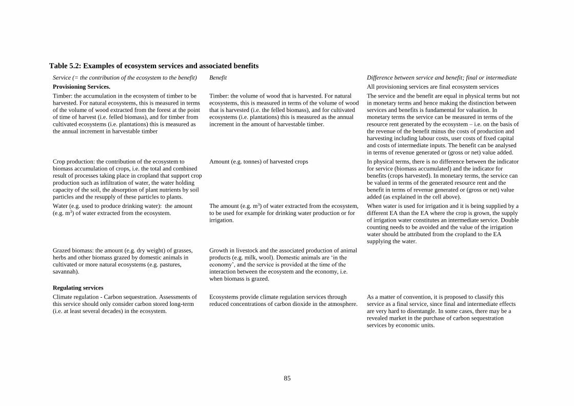
85

Table 5.2: Examples of ecosystem services and associated benefits

Service (= the contribution of the ecosystem to the benefit) Benefit Difference between service and benefit; final or intermediate

Provisioning Services. All provisioning services are final ecosystem services

Timber: the accumulation in the ecosystem of timber to be

harvested. For natural ecosystems, this is measured in terms

of the volume of wood extracted from the forest at the point

of time of harvest (i.e. felled biomass), and for timber from

cultivated ecosystems (i.e. plantations) this is measured as

the annual increment in harvestable timber

Timber: the volume of wood that is harvested. For natural

ecosystems, this is measured in terms of the volume of wood

that is harvested (i.e. the felled biomass), and for cultivated

ecosystems (i.e. plantations) this is measured as the annual

increment in the amount of harvestable timber.

The service and the benefit are equal in physical terms but not

in monetary terms and hence making the distinction between

services and benefits is fundamental for valuation. In

monetary terms the service can be measured in terms of the

resource rent generated by the ecosystem – i.e. on the basis of

the revenue of the benefit minus the costs of production and

harvesting including labour costs, user costs of fixed capital

and costs of intermediate inputs. The benefit can be analysed

in terms of revenue generated or (gross or net) value added.

Crop production: the contribution of the ecosystem to

biomass accumulation of crops, i.e. the total and combined

result of processes taking place in cropland that support crop

production such as infiltration of water, the water holding

capacity of the soil, the absorption of plant nutrients by soil

particles and the resupply of these particles to plants.

Amount (e.g. tonnes) of harvested crops In physical terms, there is no difference between the indicator

for service (biomass accumulated) and the indicator for

benefits (crops harvested). In monetary terms, the service can

be valued in terms of the generated resource rent and the

benefit in terms of revenue generated or (gross or net) value

added (as explained in the cell above).

Water (e.g. used to produce drinking water): the amount

(e.g. m3) of water extracted from the ecosystem.

The amount (e.g. m3) of water extracted from the ecosystem,

to be used for example for drinking water production or for

irrigation.

When water is used for irrigation and it is being supplied by a

different EA than the EA where the crop is grown, the supply

of irrigation water constitutes an intermediate service. Double

counting needs to be avoided and the value of the irrigation

water should be attributed from the cropland to the EA

supplying the water.

Grazed biomass: the amount (e.g. dry weight) of grasses,

herbs and other biomass grazed by domestic animals in

cultivated or more natural ecosystems (e.g. pastures,

savannah).

Growth in livestock and the associated production of animal

products (e.g. milk, wool). Domestic animals are ‘in the

economy’, and the service is provided at the time of the

interaction between the ecosystem and the economy, i.e.

when biomass is grazed.

Regulating services

Climate regulation - Carbon sequestration. Assessments of

this service should only consider carbon stored long-term

(i.e. at least several decades) in the ecosystem.

Ecosystems provide climate regulation services through

reduced concentrations of carbon dioxide in the atmosphere.

As a matter of convention, it is proposed to classify this

service as a final service, since final and intermediate effects

are very hard to disentangle. In some cases, there may be a

revealed market in the purchase of carbon sequestration

services by economic units.

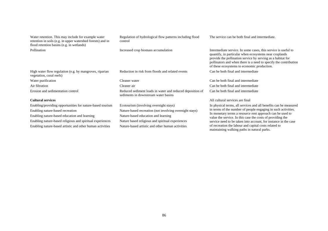
86

Water retention. This may include for example water

retention in soils (e.g. in upper watershed forests) and in

flood retention basins (e.g. in wetlands)

Regulation of hydrological flow patterns including flood

control

The service can be both final and intermediate.

Pollination Increased crop biomass accumulation Intermediate service. In some cases, this service is useful to

quantify, in particular when ecosystems near croplands

provide the pollination service by serving as a habitat for

pollinators and when there is a need to specify the contribution

of these ecosystems to economic production.

High water flow regulation (e.g. by mangroves, riparian

vegetation, coral reefs)

Reduction in risk from floods and related events Can be both final and intermediate

Water purification Cleaner water Can be both final and intermediate

Air filtration Cleaner air Can be both final and intermediate

Erosion and sedimentation control Reduced sediment loads in water and reduced deposition of

sediments in downstream water basins

Can be both final and intermediate

Cultural services All cultural services are final

Enabling/providing opportunities for nature-based tourism Ecotourism (involving overnight stays) In physical terms, all services and all benefits can be measured

in terms of the number of people engaging in such activities.

In monetary terms a resource rent approach can be used to

value the service. In this case the costs of providing the

service need to be taken into account, for instance in the case

of recreation the labour and capital costs related to

maintaining walking paths in natural parks.

Enabling nature-based recreation Nature-based recreation (not involving overnight stays)

Enabling nature-based education and learning Nature-based education and learning

Enabling nature-based religious and spiritual experiences Nature based religious and spiritual experiences

Enabling nature-based artistic and other human activities Nature-based artistic and other human activities

87

5.5 The role and use of biophysical modelling

5.5.1 Introduction

5.83. Biophysical modelling, in the context of this guidance document, is defined as

the modelling of biological and/or physical processes in order to understand the

biophysical elements to be recorded in an ecosystem account. These elements are part

of either ecosystem asset measurement (including ecosystem condition and the

ecosystem’s capacity to generate services) or ecosystem services measurement. In this

chapter, the focus is on ecosystem services.

5.84. The intention here is to provide some general guidance on the types of

biophysical modelling approaches that can be used to analyse ecosystem service flows,

as distinct from models that can be used to understand ecosystem processes (e.g.

nutrient cycling, energy flows). In the scientific literature, a wide range of different

modelling approaches has been described in the fields of ecology, geography and

hydrology. Many of them are potentially relevant to ecosystem accounting depending

upon the environmental characteristics, the uses of the ecosystem, the scale of the

analysis, and the available data. It is impossible to describe all these different modelling

approaches in one document. This section provides an overview of the different

approaches, and their main uses for the biophysical modelling of ecosystem services.

5.85. An important aspect of applying biophysical models in ecosystem accounting

is recognising the nature of the connections between ecosystem service flows and the

condition of the relevant ecosystem asset. This connection is reflected in the concept

of ecosystem capacity. Although the definition of ecosystem capacity remains a matter

of ongoing discussion (see section 7.3), it is accepted broadly, that modelling

ecosystem service flows must take into consideration the current and expected future

condition of the ecosystem and its various functions and processes.

5.5.2 Overview of biophysical modelling approaches

5.86. Ecosystem accounting will generally involve a combination of spatial and

spatial-temporal modelling approaches. Spatial modelling is required to produce maps

of ecosystem services for a complete ecosystem accounting area. Spatial modelling is

most commonly undertaken using GIS packages such as ArcGIS© and Quantum GIS.

5.87. There are also several ecosystem services specific modelling tools such as

ARIES, MIMES, LUCI and InVEST (see e.g. Bagstad et al., 2013 for an overview and

comparison of modelling tools). Several assessments of the relative strengths of these

modelling tools have been published. In general, the tools differ in terms of

sophistication, ease of use, capacity to handle large volumes of data, and alignment

with the SEEA EEA framework.

5.88. Within the general GIS packages, spatial modelling tools that can be used to

produce ecosystem services maps include look-up tables and interpolation techniques

such as inverse distance weighting and kriging. In addition, specific GIS extensions

such as Maximum Entropy modelling (Maxent) (Philips, et al., 2006) can be used.

Lookup tables attribute specific values (e.g. of the amount of service supplied per

hectare) to each EA. Inverse distance weighting algorithms are deterministic and

predict values of un-sampled points based on measured values of nearby points.

Kriging and Maxent use statistical algorithms to predict the value of un-sampled pixels.

Kriging considers distance to sampled points as well as statistical relationships between

sampled points in the interpolation, and Maxent predicts values for un-sampled pixels

on the basis of the characteristics of the pixels. Maxent has traditionally been used to

88

predict the occurrence of specific species based on characteristics such as ecosystem

type, ecosystem condition and distance to human settlements and roads. Critical in

applying geostatistics is that a sufficiently large sample size is available, and that

samples are representative of the overall spatial variability found. Examples of the

applications of these approaches can be found in, for example, Karl (2010) in a study

on rangeland ecosystem condition and Remme, et al. (2014) in a study of ecosystem

services.

5.89. In ecosystem accounting, modelling is required to estimate the potential and

capacity of an ecosystem to generate ecosystem services. The modelling approach that

is consistent with coming to an understanding of flows of ecosystem services over time

is a dynamic systems approach, which can also be applied in combination with spatial

models. A dynamic systems approach is based upon modelling a set of state (level) and

flow (rate) variables in order to capture the state of the ecosystem over time, including

relevant inputs, throughputs and outputs. Dynamic systems models use a set of

equations linking ecosystem condition or state, management and flows of services. For

instance, a model may include the amount of standing biomass (state), regeneration of

wood (flow), the harvest of wood (flow), and the price of wood (time dependent

variable).

5.90. A systems approach can contain non-linear dynamic processes, feedback

mechanisms and control strategies, and can therefore deal with complex ecosystem

dynamics. However, it is often a challenge to understand these complex dynamics, and

their spatial variability, and data shortages may be a concern for ecosystem accounting

that requires large scale analysis of ecosystem dynamics and flows of ecosystem

services. In addition, operating costs and data requirements may be prohibitive to

model a broad range of ecosystems services at fine resolution and in large areas. A

potential way forward is to be selective in applying temporal models, e.g. by limiting

modelling efforts to services that shown downward trends, and assume constant flows

in time, at least initially, for services where such trends are not apparent.

5.91. Erosion and erosion control resulting from vegetation cover are often modelled

with the USLE (Universal Soil Loss Equation), although its reliability in environments

other than the landscapes and slope types for which it was developed (the United States)

has proven to be variable. Other examples of process based models are the hydrological

models such as SWAT (Soil and Water Assessment Tool) and SedNet from the

Australian Commonwealth Scientific and Industrial Research Organisation (CSIRO).

These models are both temporally and spatially explicit, and use a modelling approach

integrated in a GIS environment.

5.92. If no data for specific ecosystem service flows is available, new data

collection/generation (including inventories, remote sensing, spatial modelling and

other sources) may be required. Data collection should be developed in a way that

provides consistent estimates across the different service types (e.g. of similar detail,

quality, error and uncertainties), as well as correctly embedded in the ecological and

land use processes. Alternative modelling tools include:

• For soil and water-related process and service modelling tools consider SWAT,

SedNet and others

• For carbon-related process and service modelling tools consider CASA (Potter,

1993), MODIS (MOD17) algorithm (Running, Nemani et al, 2004), BiomeBGC

(Turner, Ritts et al, 2011) ORCHIDEE (Ciais, Wattenbach et al, 2010) and others

• For biodiversity and other service modelling tools where extrapolations of point

(presence) data are relevant consider Maxent and others as described in Chapter 9.

89

5.6 Data sources, materials and methods for measuring ecosystem service flows

5.6.1 Introduction

5.93. SEEA EEA Annex A3 provides some stylised figures to help articulate the

measurement required to estimate flows of ecosystem services. The figures included in

that annex only relate to selected services but the basic logic of the models can be

applied more generally. Of particular importance is recognising the distinction between

the ecosystem service and the associated benefit.

5.94. Generally, it will be helpful for measurement purposes to distinguish between

provisioning, regulating and cultural services. For this task, the use of a classification

of ecosystem services, such as those described above, can serve as a useful checklist.

Further, it is likely to be useful to consider the measurement of ecosystem services in

relation to ecosystem types such as forests, wetlands, and agricultural areas.

5.95. A useful structuring of indicators is presented in Chapter 5 of the European

Union’s MAES project report (Maes et al., 2014). It presents indicators for different

ecosystem services mapped across four broad ecosystem types – forest, cropland and

grassland, freshwater and marine. A review of this material highlights the likely broad

range of data sources that will need to be considered in generating a full coverage of

ecosystem services.

5.6.2 Data sources

5.96. Data sources will be different in each country. It is suggested that important

national data holders be engaged in the process of compiling the accounts. They will

be able to advise on data availability and quality. The following list suggests some

government departments (using generic titles) and the data they may hold:

• National Statistical Offices: agricultural production (crops and livestock); health

statistics (incidence of environmentally-related diseases), population data,

tourism data;

• Meteorological Agencies: rainfall, temperature, climate variables

• Departments of Natural Resources: timber stock and harvest; biomass harvest

for energy; water supply and consumption; natural disaster statistics (floods,

landslides, storms); land cover (to estimate carbon stock and sequestration);

remote sensing (to estimate primary production);

• Water management and related agencies: water stocks and flows, abstraction

rates, data from hydrological modeling;

• Departments of Agriculture: crop production, use of inputs in agriculture,

erosion potential, biomass harvest;

• Departments of Forestry: forest stock and harvest; growth rates of forests, carbon

sequestration;

• Departments of Environment and Parks: Iconic species habitats, visitors to

natural areas, biodiversity.

5.97. Where national data are lacking, global datasets may be used. For instance,

there are now several global datasets on soils such as the Harmonized World Soil

Database and the ISRIC-WISE 3.1 soil profile database as well as global datasets on

soil properties derived from these datasets (e.g. Stoorvogel, et al., 2016). There is also

a global Digital Elevation Model that can be downloaded

(http://www.gisat.cz/content/en/products/digital-elevation-model/aster-gdem) as well

90

as several global datasets on forest cover, for instance from the Global Forest Watch.

MODIS provides satellite derived, global information on a range of land, vegetation

and water-related indicators at 250 to 1000m grid size, often multiple times per year

(https://modis.gsfc.nasa.gov/). WaterWorld provides global information on various

hydrological properties including rainfall and potential evapotranspiration at a 1 ha to

1 km2 resolution (http://www.policysupport.org/waterworld). However, the accuracy

of these products may typically be lower than national datasets and care needs to be

taken in applying such datasets for national scale analyses (where feasible involving

validation of the datasets).

5.98. Local academic and government researchers may have conducted studies for

specific regions of the country or for specific services. As well, international

organizations (e.g. UNEP, Secretariat for the CBD, World Bank) may have conducted

studies on specific locations or services. These should also be reviewed and considered

for integration into the ecosystem services supply and use account.

5.99. Databases storing research on ecosystem valuation will also include

information on the physical aspects of the ecosystems they value. For example, if the

fish harvest in one lake is estimated to generate US$50,000 per year, the research is

likely to also include estimates of fish yields in physical units.

5.100. Two broad based ecosystem valuation databases that can be investigated for

country-specific (or region-specific) biophysical data are the EVRI (Environmental

Valuation Reference Inventory, at www.evri.ca) and the ESVD (Ecosystem Service

Valuation Database at http://www.fsd.nl/esp/80763/5/0/50) that emerged from the

TEEB (2010) study. Other service-specific or region-specific databases or projects

should also be investigated. Note that the monetary valuations from these databases

may not be appropriate for accounting purposes depending on the valuation concept

applied (see discussion in Chapter 6).

5.101. In some cases, data may be available at a fine level of spatial detail, for

example from an agricultural census. In other cases, it may be necessary, if sub-national

accounts are to be compiled, to allocate national or regional level estimates to the

spatial areas being used for ecosystem accounting using spatial modelling techniques.

5.102. Depending on the resources, including time available, it may be feasible to

collect new data. New data collection activities could include:

• Ecological field studies to determine location-specific supply of ecosystem

services. Such studies could, for example, collect data on water purification

services of wetlands.

• Socio-economic surveys could be conducted to better understand how people

and businesses use and value ecosystem services (e.g., water withdrawals,

visits to recreational sites)

• Case studies could be conducted on target populations (e.g., households near

forest areas) to better understand their use of ecosystem services (e.g., biomass

for fuel, food gathering, sources of water).

5.103. While there is an increasing amount of information and examples of

measurement of ecosystem service flows, a challenge is likely to lie in adapting,

integrating and scaling the available information from multiple sources for ecosystem

accounting purposes. The issue of scaling is considered below. From a practical

perspective, it is sufficient to note here that, when accounting for multiple ecosystem

services, the aim must be to measure the supply of ecosystem services for multiple

ecosystem assets and types, and also over a series of accounting periods. As

appropriate, adjustments to ensure that measures of different ecosystem services relate

to common spatial areas and the same time periods should be made.

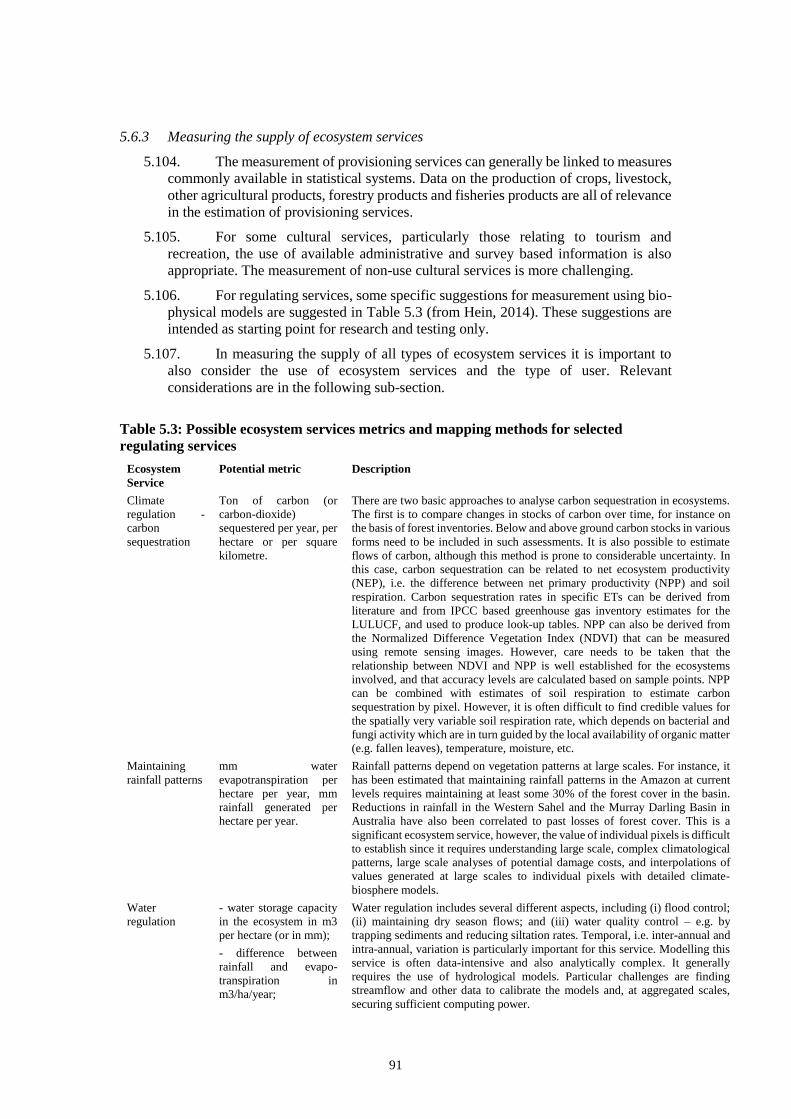
91

5.6.3 Measuring the supply of ecosystem services

5.104. The measurement of provisioning services can generally be linked to measures

commonly available in statistical systems. Data on the production of crops, livestock,

other agricultural products, forestry products and fisheries products are all of relevance

in the estimation of provisioning services.

5.105. For some cultural services, particularly those relating to tourism and

recreation, the use of available administrative and survey based information is also

appropriate. The measurement of non-use cultural services is more challenging.

5.106. For regulating services, some specific suggestions for measurement using bio-

physical models are suggested in Table 5.3 (from Hein, 2014). These suggestions are

intended as starting point for research and testing only.

5.107. In measuring the supply of all types of ecosystem services it is important to

also consider the use of ecosystem services and the type of user. Relevant

considerations are in the following sub-section.

Table 5.3: Possible ecosystem services metrics and mapping methods for selected

regulating services

Ecosystem

Service

Potential metric Description

Climate

regulation -

carbon

sequestration

Ton of carbon (or

carbon-dioxide)

sequestered per year, per

hectare or per square

kilometre.

There are two basic approaches to analyse carbon sequestration in ecosystems.

The first is to compare changes in stocks of carbon over time, for instance on

the basis of forest inventories. Below and above ground carbon stocks in various

forms need to be included in such assessments. It is also possible to estimate

flows of carbon, although this method is prone to considerable uncertainty. In

this case, carbon sequestration can be related to net ecosystem productivity

(NEP), i.e. the difference between net primary productivity (NPP) and soil

respiration. Carbon sequestration rates in specific ETs can be derived from

literature and from IPCC based greenhouse gas inventory estimates for the

LULUCF, and used to produce look-up tables. NPP can also be derived from

the Normalized Difference Vegetation Index (NDVI) that can be measured

using remote sensing images. However, care needs to be taken that the

relationship between NDVI and NPP is well established for the ecosystems

involved, and that accuracy levels are calculated based on sample points. NPP

can be combined with estimates of soil respiration to estimate carbon

sequestration by pixel. However, it is often difficult to find credible values for

the spatially very variable soil respiration rate, which depends on bacterial and

fungi activity which are in turn guided by the local availability of organic matter

(e.g. fallen leaves), temperature, moisture, etc.

Maintaining

rainfall patterns

mm water

evapotranspiration per

hectare per year, mm

rainfall generated per

hectare per year.

Rainfall patterns depend on vegetation patterns at large scales. For instance, it

has been estimated that maintaining rainfall patterns in the Amazon at current

levels requires maintaining at least some 30% of the forest cover in the basin.

Reductions in rainfall in the Western Sahel and the Murray Darling Basin in

Australia have also been correlated to past losses of forest cover. This is a

significant ecosystem service, however, the value of individual pixels is difficult

to establish since it requires understanding large scale, complex climatological

patterns, large scale analyses of potential damage costs, and interpolations of

values generated at large scales to individual pixels with detailed climate-

biosphere models.

Water

regulation

- water storage capacity

in the ecosystem in m3

per hectare (or in mm);

- difference between

rainfall and evapo-

transpiration in

m3/ha/year;

Water regulation includes several different aspects, including (i) flood control;

(ii) maintaining dry season flows; and (iii) water quality control – e.g. by

trapping sediments and reducing siltation rates. Temporal, i.e. inter-annual and

intra-annual, variation is particularly important for this service. Modelling this

service is often data-intensive and also analytically complex. It generally

requires the use of hydrological models. Particular challenges are finding

streamflow and other data to calibrate the models and, at aggregated scales,

securing sufficient computing power.

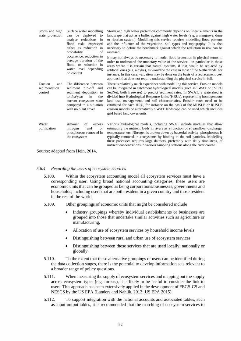
92

Storm and high

water protection

Surface water modelling

can be deployed to

analyse reductions in

flood risk, expressed

either as reduction in

probability of

occurrence, reduction in

average duration of the

flood, or reduction in

water level depending

on context

Storm and high water protection commonly depends on linear elements in the

landscape that act as a buffer against high water levels (e.g. a mangrove, dune

or riparian system). Modelling this service requires modelling flood patterns

and the influence of the vegetation, soil types and topography. It is also

necessary to define the benchmark against which the reduction in risk can be

assessed.

It may not always be necessary to model flood protection in physical terms in

order to understand the monetary value of the service - in particular in those

areas where it is certain that natural systems, if lost, would be replaced by

artificial ones (e.g. a dyke), as would be the case in most of the Netherlands, for

instance. In this case, valuation may be done on the basis of a replacement cost

approach that does not require understanding the physical service in full.

Erosion and

sedimentation

control

The difference between

sediment run-off and

sediment deposition in

ton/ha/year in the

current ecosystem state

compared to a situation

with no plant cover

There is relatively much experience with modelling this service. Erosion models

can be integrated in catchment hydrological models (such as SWAT or CSIRO

SedNet, both freeware) to predict sediment rates. In SWAT, a watershed is

divided into Hydrological Response Units (HRUs), representing homogeneous

land use, management, and soil characteristics. Erosion rates need to be

estimated for each HRU, for instance on the basis of the MUSLE or RUSLE

erosion models or alternatively SWAT landscape can be used which includes

grid based land cover units.

Water

purification

Amount of excess

nitrogen and or

phosphorous removed in

the ecosystem

Various hydrological models, including SWAT include modules that allow

estimating the nutrient loads in rivers as a function of streamflow, discharge,

temperature, etc. Nitrogen is broken down by bacterial activity, phosphorous is

typically removed in ecosystems by binding to the soil particles. Modelling

these processes requires large datasets, preferably with daily time-steps, of

nutrient concentrations in various sampling stations along the river course.

Source: adapted from Hein, 2014.

5.6.4 Recording the users of ecosystem services

5.108. Within the ecosystem accounting model all ecosystem services must have a

corresponding user. Using broad national accounting categories, these users are

economic units that can be grouped as being corporations/businesses, governments and

households, including users that are both resident in a given country and those resident

in the rest of the world.

5.109. Other groupings of economic units that might be considered include

• Industry groupings whereby individual establishments or businesses are

grouped into those that undertake similar activities such as agriculture or

manufacturing.

• Allocation of use of ecosystem services by household income levels

• Distinguishing between rural and urban use of ecosystem services

• Distinguishing between those services that are used locally, nationally or

globally.

5.110. To the extent that these alternative groupings of users can be identified during

the data collection stages, there is the potential to develop information sets relevant to

a broader range of policy questions.

5.111. When measuring the supply of ecosystem services and mapping out the supply

across ecosystem types (e.g. forests), it is likely to be useful to consider the link to

users. This approach has been extensively applied in the development of FEGS-CS and

NESCS by the US EPA (Landers and Nahlik, 2013; US EPA 2015).

5.112. To support integration with the national accounts and associated tables, such

as input-output tables, it is recommended that the matching of ecosystem services to

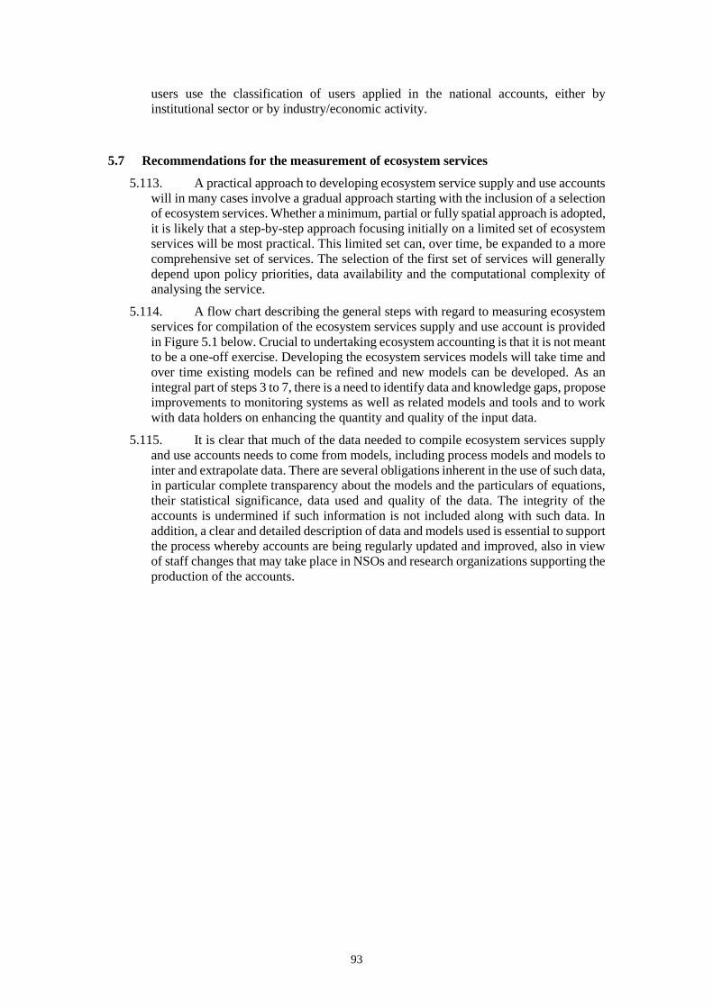
93

users use the classification of users applied in the national accounts, either by

institutional sector or by industry/economic activity.

5.7 Recommendations for the measurement of ecosystem services

5.113. A practical approach to developing ecosystem service supply and use accounts

will in many cases involve a gradual approach starting with the inclusion of a selection

of ecosystem services. Whether a minimum, partial or fully spatial approach is adopted,

it is likely that a step-by-step approach focusing initially on a limited set of ecosystem

services will be most practical. This limited set can, over time, be expanded to a more

comprehensive set of services. The selection of the first set of services will generally

depend upon policy priorities, data availability and the computational complexity of

analysing the service.

5.114. A flow chart describing the general steps with regard to measuring ecosystem

services for compilation of the ecosystem services supply and use account is provided

in Figure 5.1 below. Crucial to undertaking ecosystem accounting is that it is not meant

to be a one-off exercise. Developing the ecosystem services models will take time and

over time existing models can be refined and new models can be developed. As an

integral part of steps 3 to 7, there is a need to identify data and knowledge gaps, propose

improvements to monitoring systems as well as related models and tools and to work

with data holders on enhancing the quantity and quality of the input data.

5.115. It is clear that much of the data needed to compile ecosystem services supply

and use accounts needs to come from models, including process models and models to

inter and extrapolate data. There are several obligations inherent in the use of such data,

in particular complete transparency about the models and the particulars of equations,

their statistical significance, data used and quality of the data. The integrity of the

accounts is undermined if such information is not included along with such data. In

addition, a clear and detailed description of data and models used is essential to support

the process whereby accounts are being regularly updated and improved, also in view

of staff changes that may take place in NSOs and research organizations supporting the

production of the accounts.

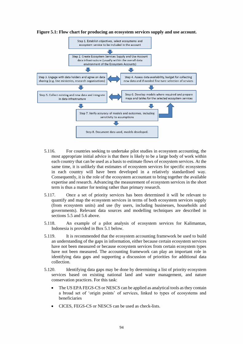
94

Figure 5.1: Flow chart for producing an ecosystem services supply and use account.

5.116. For countries seeking to undertake pilot studies in ecosystem accounting, the

most appropriate initial advice is that there is likely to be a large body of work within

each country that can be used as a basis to estimate flows of ecosystem services. At the

same time, it is unlikely that estimates of ecosystem services for specific ecosystems

in each country will have been developed in a relatively standardised way.

Consequently, it is the role of the ecosystem accountant to bring together the available

expertise and research. Advancing the measurement of ecosystem services in the short

term is thus a matter for testing rather than primary research.

5.117. Once a set of priority services has been determined it will be relevant to

quantify and map the ecosystem services in terms of both ecosystem services supply

(from ecosystem units) and use (by users, including businesses, households and

governments). Relevant data sources and modelling techniques are described in

sections 5.5 and 5.6 above.

5.118. An example of a pilot analysis of ecosystem services for Kalimantan,

Indonesia is provided in Box 5.1 below.

5.119. It is recommended that the ecosystem accounting framework be used to build

an understanding of the gaps in information, either because certain ecosystem services

have not been measured or because ecosystem services from certain ecosystem types

have not been measured. The accounting framework can play an important role in

identifying data gaps and supporting a discussion of priorities for additional data

collection.

5.120. Identifying data gaps may be done by determining a list of priority ecosystem

services based on existing national land and water management, and nature

conservation practices. For this task:

• The US EPA FEGS-CS or NESCS can be applied as analytical tools as they contain

a broad set of ‘origin points’ of services, linked to types of ecosystems and

beneficiaries

• CICES, FEGS-CS or NESCS can be used as check-lists.

95

5.121. Depending on the nature of the data gaps, the use of benefit transfer functions

may be considered and cautiously tested. Generally, it will be important to develop an

understanding of uncertainties when defining, classifying, quantifying and mapping

ecosystem services and to prepare validation/quality control data and protocols.

5.8 Key areas for research

5.122. Notwithstanding the priority for testing to be the focus of current activity, there

are some areas of research that would support this testing work. Primary among these

is resolution of issues concerning the definition and classification of ecosystem

services. This work has advanced well and the relevant boundary issues are quite well

delineated. However, further consultation leading to decisions or treatments is needed

to put in place a classification of ecosystem services that is, at least, appropriate for

ecosystem accounting purposes.

5.123. The second key area of research is articulation of the treatment and

measurement of intermediate services in ecosystem accounting. A related task is

specifying what are best called ecological production functions or value chains – i.e.

the sequence of ecosystem processes, possibly across ecosystem types, that leads to the

supply of a final ecosystem service. Although it is not anticipated that a complete

catalogue of all such production functions would be established in the short to medium

term, research in this direction would be of direct benefit to applying ecosystem

services and ecosystem accounting measures to policy questions. Examples of relevant

ecological processes include rates of growth (e.g. of timber), decomposition, soil

erosion, habitat fragmentation, water runoff and yield.

Box 5.1: Ecosystem services mapping in Central Kalimantan

In a 2014 PhD project at Wageningen

University, seven ecosystem services were

mapped following the SEEA EEA in Central

Kalimantan province, Indonesia for the year

2010. Mapping the seven selected ecosystem

services required a specific dataset for each

service. The data were collected from a variety

of sources including from existing land cover

maps soil maps, Digital Elevation Models,

topographic and hydrological maps. The land

cover map, topographic map, and hydrological

map are available in vector format. All spatial

input data were converted to raster format with

a pixel size of 100 m for further spatial analysis.

Spatial data were combined with Indonesian

statistical data on rice, timber, and palm oil

production. Furthermore, survey data from

various published studies were used to analyse

rattan cultivation, tourism and rice production,

and company data were used for timber

production. The services were connected to a

land cover map from 2010, and as much as

possible ecosystem services data from 2010 was

used. However, for some services data from

2009 or 2011 was used as a proxy. The map

below specifies ecosystem services supply in

Central Kalimantan in 2010.

In constructing the map, it was found that

ecosystem services supply could not be related

to a set of ecosystem properties (including soil,

rainfall, slope, soil, and vegetation biomass)

with sufficient reliability (typically R2<0.2 for

all provisioning services). The explanation for

this may be that there is no strong correlation

between ecosystem properties and extraction

rates of provisioning services, and that

extraction rates are an overriding factor that

determine flows of provisioning services.

Therefore, in order to produce wall-to-wall

mapping of ecosystem services, different spatial

modelling techniques were used. These

included lookup tables, interpolation,

regression modelling, and probabilistic models

such as Maxent.

Provisioning services are commonly supplied in

only one land cover class, but within these land

cover classes there can be substantial variation

in supply. Provisioning services were therefore

mapped using spatial interpolation instead of

using lookup tables (which results in a specific

value for a given land use class). Interpolation

was carried out in ArcGIS using ordinary

kriging. Note that the habitat service is included

as a service in the map, expressing both

biodiversity and potential to support tourism.

This service was mapped with Maxent. For

carbon, there were insufficient observations to

pursue spatial interpolation, even though it is

likely that spatial variation within ecosystem

types also occurs. Therefore, for carbon

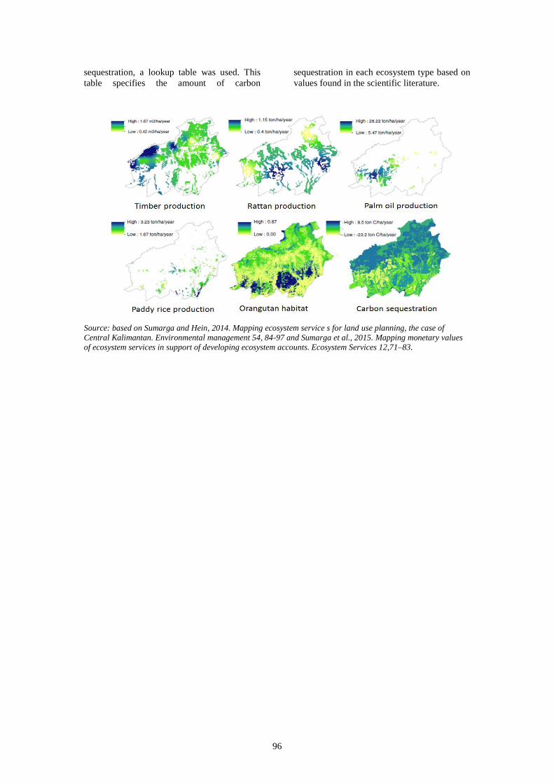
96

sequestration, a lookup table was used. This

table specifies the amount of carbon

sequestration in each ecosystem type based on

values found in the scientific literature.

Source: based on Sumarga and Hein, 2014. Mapping ecosystem service s for land use planning, the case of

Central Kalimantan. Environmental management 54, 84-97 and Sumarga et al., 2015. Mapping monetary values

of ecosystem services in support of developing ecosystem accounts. Ecosystem Services 12,71–83.

97

6 Valuation in ecosystem accounting

Key points in this chapter

The estimation of monetary values for ecosystem services and ecosystem assets can be undertaken for a

variety of purposes. It is essential that the purpose of valuation is well understood.

In ecosystem accounting, the primary purpose of valuation in monetary terms is the integration of

information on ecosystem condition and ecosystem services with information in the standard national

accounts. This provides information to support comparison of ecosystem services with the production

and consumption of other goods and services and supports the use of ecosystem information in standard

economic modelling and productivity analysis.

For this purpose, the valuation concepts and approaches used for ecosystem accounting need to be

consistent with the valuation concept used in the national accounts – i.e. exchange values. Exchange

values are those values that reflect the price at which ecosystem services and ecosystem assets would be

exchanged between buyer and seller if a market existed.

For other policy and analytical purposes, different valuation concepts will be appropriate including the

estimation of welfare based values and the use of non-monetary valuation techniques. Although these

valuation concepts should not be applied to derive monetary valuations for ecosystem accounting, the

broader ecosystem accounting model showing the relationships between ecosystem assets, their

condition and the services supplied will still be relevant. Wherever possible a common underlying dataset

on ecosystem stocks and flows in physical terms should be used to underpin valuation studies,

irrespective of the valuation concept and purpose being applied.

Recent investigation into the potential to use the range of non-market environmental valuation techniques

suggests that many are relevant or may be adapted for use in accounting. Nonetheless, much further

discussion and testing on the use of valuation methods for the estimation of exchange values is required.

In ecosystem accounting, the valuation of ecosystem services is the starting point for the valuation of

ecosystem assets. A clear distinction should be made between these two objects of valuation.

6.1 Introduction

6.1. The issue of valuation can complicate the discussion of ecosystem and natural

capital accounting. This occurs for many reasons. For some, the concerns about

valuation relate to the implication that a “dollar value” is placed on all environmental

assets and services and that this is both inappropriate and misleading. For others, the

measurement concerns are too great and the environment is considered too complex to

suggest that useful measures in monetary terms might be compiled. Finally, there are

differences concerning the purposes, concepts and techniques in relation to monetary

valuation.

6.2. As in SEEA EEA chapter 5, the ambition in this chapter is to provide a possible

pathway through these various issues, such that the discussion on valuation for

ecosystem accounting can be placed in context with other approaches and perspectives.

6.3. One general conclusion is that valuation in monetary terms requires careful

consideration of the purpose of the valuation. Alternative purposes include accounting

purposes and the assessment of changes in welfare between alternative scenarios. Once

the purpose is defined, the appropriate valuation concept can be selected and from this,

the relevant valuation method and technique can be applied. Often the discussion in

environmental valuation moves directly to discussion of method and technique without

recognising that different purposes for valuation, and hence different valuation

concepts may be relevant.

6.4. It is clear that the majority of work in this area of valuation has been motivated

by the assessment of trade-offs between different potential land uses and in this context

98

monetary valuation of ecosystem services has a particular interest in measuring

differences in economic surplus associated with different scenarios, following a

standard cost-benefit type methodology. Other work has been focused on the

measurement of shadow prices for ecosystem assets taking into account relevant

externalities. Given these analytical perspectives for many involved in the ecosystem

services valuation space, the focus on exchange values of ecosystem services for

accounting purposes may appear inappropriate or irrelevant.

6.5. However, accounting is designed to support a different analytical and policy

perspective, in particular to encourage and support the use of environmental

information in standard economic and financial decision making. In this context, the

measurement of the value of ecosystem services in exchange values support direct

integration with standard financial and national economic accounting data.

Consequently, the data can be used directly to extend standard economic modelling

approaches and to enhance broad indicators of economic performance such as national

income, savings and productivity. While these measures and applications are different

from the more common applications of ecosystem services valuations, the ability to

consider ecosystems through multiple analytical lenses appears a strong motivation to

continue development of valuations for accounting purposes.

6.6. A fundamental aspect of valuation in an accounting context is that the first step

is the valuation of individual ecosystem services. In general, this will require finding

an appropriate monetary value to apply to an imputed exchange of (or transaction in)

ecosystem services between a given ecosystem asset (e.g. a forest) and an economic

unit (e.g. a forestry company) or individual (e.g. visitor to a forest).

6.7. Valuing ecosystem assets is a distinct task. For a comprehensive valuation, it

requires estimation of the future flows of ecosystem services that are expected to be

supplied by an ecosystem asset. In some cases, for example agricultural land, observed

market values for land will be able to be related to the value of ecosystem assets but

these prices will likely include non-ecosystem related values (e.g. the potential of land

for development) but also omit non-marketed ecosystem services (e.g. water regulation

services). Thus, the valuation of ecosystem assets goes beyond the step of valuing

individual ecosystem services.

6.8. This chapter is structured in the following way. In section 6.2 the main

valuation principles for ecosystem accounting are outlined drawing out the key points

from the material presented in SEEA EEA chapter 5 and incorporating a range of

considerations that have emerged since that time. Section 6.3 considers relevant data

and source materials and in section 6.4 the key challenges in valuation are described.

The final section provides a summary of recommendations in relation to valuation

based on current practice and knowledge and a summary of the key issues requiring

further research. Recognising the distinct nature of the task of valuing ecosystem asset,

the issues related to the valuation of ecosystem assets and the valuation of ecosystem

degradation are discussed in Chapter 7.

6.2 Valuation principles for ecosystem accounting

6.2.1 Introduction

6.9. SEEA EEA recognises that the term valuation can mean different things. For

accountants and economists, valuation is almost always used in the context of placing

a monetary value on assets, goods or services. In other contexts, valuation may refer to

a more general notion of recognising significance or importance. In SEEA EEA, the

focus is on valuation in monetary terms but this is not to discount the role or importance

of other concepts of value. Indeed, accounting for ecosystem condition and ecosystem

99

services in physical terms may provide a relevant information base for non-monetary

valuation. (A useful introduction to different concepts of valuation including both

monetary and non-monetary valuation is provided in IPBES (Pascual, et al., 2017), see

also Maynard et al. (2014)).

6.10. Monetary valuation in the SEEA EEA is applied to the valuation of ecosystem

services and the valuation of ecosystem assets. The relevant valuation concept for

ecosystem accounting is exchange values. 27 If there were observable markets in

individual ecosystem services, an exchange value would reflect the prices paid by users

of ecosystem services to the relevant producers (i.e. the ecosystem assets). Since many

transactions with ecosystems are usually not reflected in observed exchanges of money,

these exchange values must be estimated using non-market valuation techniques. There

are some exceptions where payments are made to owners of resources (e.g. stumpage

fees paid by the forestry industry) and depending on the nature of the payments these

may reflect values for associated ecosystem services.

6.11. The development of techniques for non-market environmental valuation is

well-established and broad ranging. The extent of development is reflected in key

publications including Freeman (2013) and Champ et al. (2017). From a national

accounts perspective, the work on environmental valuation has commonly been

characterised as inappropriate because the techniques are often applied to answer

questions concerning the change in welfare associated with different environmental

situations. Indeed, the SEEA EEA adopted this characterisation in aligning

environmental valuation with the estimation of welfare values, a concept distinct from

exchange values required for accounting.

6.12. As the discussion between experts in environmental valuation and national

accountants has progressed in recent years, there is clear evidence of far more common

ground that has been identified in the past. This is not to say that path forward will be

straightforward, but there are strong grounds to imagine that the research and

development in environmental valuation by economists can be adapted for use in

accounting contexts. Research to understand and document the common ground and

remaining challenges is currently underway in the context of a World Bank WAVES

project. A paper examining the connections between these two perspectives on

valuation has been prepared as part of the WAVES Partnership program of work

(Atkinson and Obst, 2017). This chapter picks up on some of its key findings,

recognising that further discussion and investigation will be required.

6.2.2 Establishing the markets for exchange values

6.13. As noted, underpinning the estimation of exchange values is the notion that

there is a transaction or exchange between ecosystem assets and economic units,

businesses, governments and households, that could be imagined to take place in a

market setting. Since the ecosystem assets themselves are not actual market

participants, the challenge in valuation for accounting lies in establishing the

assumptions about the institutional arrangements that would apply if there was an

actual market involving ecosystem assets.

6.14. One way of considering this is to find parallels between existing markets and

transactions in ecosystem services. Some ecosystem services can be reasonably closely

connected to activities in markets. This is generally the case for provisioning services

where ecosystem services that contribute to the production of food, fibre, fuel and

27 The term exchange values was introduced in the SEEA EEA since the term market prices as used in the

SNA is often misunderstood to mean that national accounting only incorporates values of goods and services

transacted in markets. An alternative term for the target valuation concept is transaction price. This term

may be substituted for exchange values without loss of meaning.

100

energy can be valued using observed values for the associated marketed products. Here

a close connection can be made to the values used in the SNA to estimate production

and consumption. One description of these types of ecosystem services is that their

values are “near-market” (Nordhaus, 2006; Farley, 2008). In this context, the implicit

assumption is that the institutional arrangements underpinning the exchanges of

ecosystem services are the same as for the closely associated products.

6.15. On the other hand, many ecosystem services contribute to benefits that are not

closely connected to existing markets. Often these are ecosystem services that may be

considered to provide public goods – e.g. the contribution of ecosystems to flood

protection. In these cases, determining valuation techniques for the estimation of

exchange values is more complicated since the nature of the appropriate institutional

arrangements is not clear.

6.16. In standard national accounting, the values that are recorded do not rely on

making specific assumptions regarding institutional arrangements. That is, the national

accounts record transactions and associated values as they are revealed in exchanges

between economic units without adjustment for the nature of the underlying

institutional arrangements. Thus, national accounting records observed exchange

values equally whether in open or regulated market situations.

6.17. While being open to recording observed exchanges in all market structures,

this however does leave open the question of what institutional arrangements should

be assumed in the case of ecosystem service valuation when there is no existing market.

Generally, national accountants are relatively pragmatic in such contexts and are likely

to consider what market arrangements are most likely given the country, the likely

behaviour of market participants, existing tax and regulatory settings and the type of

ecosystem service. Since accountants will make these types of assessments looking

back in time (accounting records past events), the estimation context is somewhat

different from making these types of assumptions with respect to future behaviour or

alternative scenarios.

6.18. The key point here is to recognise that national accountants are aiming to

estimate a value that would have been revealed in the “most likely” institutional

arrangements. A useful topic for research with non-market valuation specialists would

be the description of possible institutional arrangements and assumptions under “most

likely” scenarios.

6.2.3 Estimation of changes in welfare and consumer surplus

6.19. A common application of non-market environmental valuation techniques is

the estimation of changes in welfare including producer and consumer surplus

associated with environmental externalities, both positive and negative. Since

exchange values used for national accounting explicitly exclude consumer surplus, it

has been assumed that the associated valuation techniques are inappropriate for

national accounting purposes. In fact, in estimating changes in welfare, most valuation

techniques proceed by estimating a demand curve which delineates combinations of

prices and quantities that would satisfy a given set of consumers. Conceptually,

somewhere along the demand curve lies a point at which a supplier is willing to provide

the goods or services and the intersection represents an exchange value. This line of

thinking opens up a path towards linking standard non-market environmental valuation

techniques with the requirements of national accounting. These possible connections

are described further in the following sections.

6.20. Making the connections between welfare values and accounting values will

depend on clarifying the assumptions regarding institutional arrangements. As noted

101

above, national accountants need to provide more clarity in this area to engage

effectively recognising that this is a key focus of work on non-market valuation from

an economist’s perspective. By way of example, Day (2013) observed that under the

assumption that ecosystem assets are perfectly price discriminating – i.e. as suppliers

they charge exactly what each user is willing to pay, consumer surplus is eliminated

and the estimated prices reflected in the demand curve will each be exchange values.

If such an institutional arrangement was considered reasonable for accounting this

would have material impacts on valuation for accounting purposes. Day’s observation

also highlights the need to consider assumptions concerning user and consumer

behaviour in relation to ecosystem services. In this case, there may not be support for

using this specific behavioural assumption, but the general point remains. Overall, both

economists and accountants need to consider demand and supply factors in estimating

exchange values.

6.21. One concern about the use of exchange values, and hence the exclusion of

consumer surplus is that it is likely to generate relatively lower values for ecosystem

assets which are more distant from economic units and will also not incorporate

potentially important non-use values. There are also ecosystem services where a

relatively high share of the welfare generated is in the form of consumer surplus. For

instance, in the case of air filtration an important part of the generated welfare can be

related to avoided sickness and avoided premature mortality resulting from air

pollution. In this case, the accounts would provide a lower value for this service

(notwithstanding the potential to record significant direct economic effects through

reduced health costs and productivity), compared to the higher welfare value that will

consider the value of additional life years, for example (see e.g. Remme et al., 2015 for

a detailed example).

6.22. Given the potential differences between exchange-based and welfare-based

valuation, it needs to be made very clear to the users of the accounts that the values

recorded in ecosystem accounts do not reflect welfare values and that, indeed, there

may be important deviations. Depending on the policy or decision-making context

there may therefore be a need for the estimation of both exchange-based and welfare-

based values.

6.23. This is consistent with current situation in the use of the national accounts

where monetary values also do not necessarily reflect welfare generated. For example,

the values recorded in the national accounts for the production and consumption of

education do not reflect the full welfare arising from this consumption. This is

especially so when education is provided by the public sector. The use of exchange

values to underpin macro-economic measurement and modelling is accepted, as is the

relevance of estimating welfare values in making decisions, for example in the

assessment of costs and benefits of additional investments in the education system.

6.24. Since the broad objective of ecosystem accounting is to support policy analysis

and decision making in practice, one area for further discussion and investigation is

whether a complementary set of ecosystem accounts in monetary terms might be

compiled using non-exchange value concepts. The starting logic would be that

complementary accounts could be based on the same biophysical accounts (for

ecosystem extent, condition and service flows) and then alternative valuation concepts

could be applied to support particular policy contexts. Discussion will need to consider

not only the feasibility and relevance of such an approach but also how a set of

complementary accounts would be placed in context with exchange value based

accounts.

102

6.3 Relevant data and source materials

6.3.1 Introduction

6.25. In terms of implementation, valuation exercises generally require, in the first

instance, estimation of physical flows of ecosystem services. These flows are then

multiplied by a relevant value in order to estimate the monetary value of the flows.

Information on physical flows of ecosystem services is thus of direct relevance.

6.26. In terms of estimating values, this will usually involve a combination of

approaches to analyse ecosystem services. From an aggregate perspective, the common

starting points will be information on production and income from national accounts,

economic statistics, trade data, tourism activity statistics, price index data and similar

types of statistical and administrative data. While these datasets will not provide direct

estimates of values for ecosystem services, they will provide a strong base for

understanding the relative economic significance of a range of ecosystem services

particularly provisioning services and some cultural services.

6.27. For some services, valuation requires understanding spatial patterns of

ecosystem services supply and use. This is particularly the case for regulating services.

Often, supply and use take place at distinct locations. For example, a forest may filter

air but the users of this service may be people living nearby the forest. Note that where

a fully-spatial approach is pursued, there is also the need to spatially allocate aggregate

values of services in order to produce maps of ecosystem services values (see e.g.

Remme et al., 2015 and Sumarga and Hein, 2014).

6.28. Where resources are not available to undertake primary data collection, it will

be necessary to find valuation studies that have estimated values for the relevant

ecosystem service for particular ecosystem types. There are a number of databases that

hold relevant studies, including the Ecosystem Services Valuation Database (ESVD)

that has built on the original work of the TEEB study, the Environmental Valuation

Reference Inventory (EVRI) database, and the Ecosystem Valuation Toolkit by Earth

Economics. A useful link to these and other valuation databases is on the Ecosystem

Services Partnership website (see http://www.fsd.nl/esp/80136/5/0/50).

6.29. Since the available studies do not provide a complete coverage of all locations

or all ecosystem types, the application of the results from these studies will require

careful consideration. Generally, it will be necessary to apply benefit transfer methods

in which the results from on study are applied in other contexts. The critical question

is the extent to which the contexts are comparable in terms of: (i) similarity of

ecosystem assets and their services; (ii) valuation purpose and decision context; and

(iii) similarity of likely institutional arrangements. In addition, it will be important to

understand the connection to any underlying biophysical data and the scale at which

these data have been estimated, for example, through biophysical modelling. There is

a range of approaches to benefit transfer and some are preferable to others. An

introduction to this material is provided in SEEA EEA Chapter 5 and a longer

discussion of alternative benefit transfer methods is provided in, for example Plummer

(2009) and Barton (2015).

6.30. A general caveat on the use of existing studies for the valuation of ecosystem

services (that applies equally with respect to benefit transfer approaches), is that the

materials are usually not explicit about the valuation concept being applied. Hence, it

is often unclear as to whether the approaches, estimates and recommendations are

suitable for ecosystem accounting purposes in terms of measuring exchange values.

Nonetheless, in conjunction with the discussions in SEEA EEA Chapter 5, these

materials should provide a reasonable starting point for investigating the valuation of

ecosystem services for ecosystem accounting.

103

6.31. The process outlined here for the valuation of ecosystem services can be

applied to estimate the value of ecosystem services in monetary terms for a single

ecosystem service from a single ecosystem asset or ecosystem type. However, in a

SEEA EEA context, the general ambition is to estimate values for multiple ecosystem

services across multiple ecosystem assets and ecosystem types. Where compilation

extends to this scope, then by applying the valuation techniques described in the

following sub-section, the compilation of an ecosystem services supply and use

account in monetary terms is possible. This account has the same structure as the

ecosystem services supply and use account in physical terms presented in Chapter 5,

Table 5.1. Thus, estimates for individual ecosystem services are presented together and

estimates are recorded for both the supplying ET and the receiving users. As for the

physical supply and use table it is appropriate, and likely necessary, to understand both

the supply and the use of ecosystem services to best compile this table in monetary

terms. In principle, aggregation across ecosystem services and ecosystem types is

possible even where different valuation techniques are used, provided the different

techniques are focused on measuring the same valuation concept. However, it should

be recognised that different techniques may generate substantively different estimates

of value and care should be taken in quality assuring all estimates whatever technique

is used.

6.32. Additional support for applying valuation in national accounting contexts can

be found in materials from the UNEP Ecosystem Services Economics unit, the

materials developed as part of the TEEB study, work being undertaken within the

World Bank WAVES project and the discussion of valuation in the context of the

IPBES.

6.3.2 Potential valuation techniques

6.33. A number of valuation techniques have been considered appropriate for

measuring exchange values. However, there is ongoing discussion on this topic to build

stronger levels of understanding in the use of standard non-market environmental

valuation techniques for accounting purposes. The SEEA EEA Chapter 5 outlines a

number of the techniques and an updated summary of valuation techniques is provided

in Table 6.1.

6.34. Table 6.1 presents a number of standard techniques in the left-hand column

following the structure of the discussion in the SEEA EEA. Ideally, it would be possible

to provide more specific guidance on valuation techniques by type of ecosystem service

– i.e. showing different ecosystem services in the left-hand column. At this stage, clear

advice relating to recommended valuation techniques for individual ecosystem services

has not been discussed or developed but it is the intended direction. Progress towards

this objective will be considerably supported through progress in the discussion of

classifications of ecosystem services. This will mean that a discussion on valuation

techniques can be aligned around a common description of individual ecosystem

services. It is clear that different descriptions of ecosystem services can lead to quite

alternative valuation considerations.

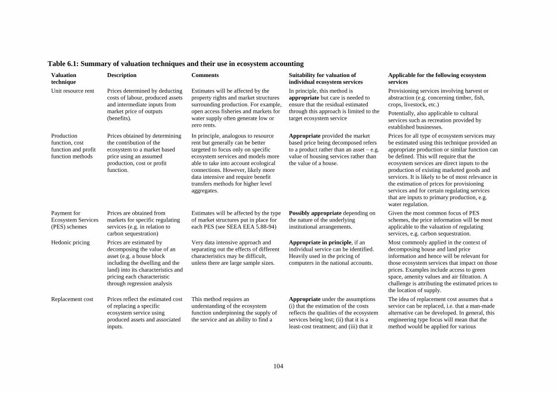
104

Table 6.1: Summary of valuation techniques and their use in ecosystem accounting

Valuation

technique

Description Comments Suitability for valuation of

individual ecosystem services

Applicable for the following ecosystem

services

Unit resource rent Prices determined by deducting

costs of labour, produced assets

and intermediate inputs from

market price of outputs

(benefits).

Estimates will be affected by the

property rights and market structures

surrounding production. For example,

open access fisheries and markets for

water supply often generate low or

zero rents.

In principle, this method is

appropriate but care is needed to

ensure that the residual estimated

through this approach is limited to the

target ecosystem service

Provisioning services involving harvest or

abstraction (e.g. concerning timber, fish,

crops, livestock, etc.)

Potentially, also applicable to cultural

services such as recreation provided by

established businesses.

Production

function, cost

function and profit

function methods

Prices obtained by determining

the contribution of the

ecosystem to a market based

price using an assumed

production, cost or profit

function.

In principle, analogous to resource

rent but generally can be better

targeted to focus only on specific

ecosystem services and models more

able to take into account ecological

connections. However, likely more

data intensive and require benefit

transfers methods for higher level

aggregates.

Appropriate provided the market

based price being decomposed refers

to a product rather than an asset – e.g.

value of housing services rather than

the value of a house.

Prices for all type of ecosystem services may

be estimated using this technique provided an

appropriate production or similar function can

be defined. This will require that the

ecosystem services are direct inputs to the

production of existing marketed goods and

services. It is likely to be of most relevance in

the estimation of prices for provisioning

services and for certain regulating services

that are inputs to primary production, e.g.

water regulation.

Payment for

Ecosystem Services

(PES) schemes

Prices are obtained from

markets for specific regulating

services (e.g. in relation to

carbon sequestration)

Estimates will be affected by the type

of market structures put in place for

each PES (see SEEA EEA 5.88-94)

Possibly appropriate depending on

the nature of the underlying

institutional arrangements.

Given the most common focus of PES

schemes, the price information will be most

applicable to the valuation of regulating

services, e.g. carbon sequestration.

Hedonic pricing Prices are estimated by

decomposing the value of an

asset (e.g. a house block

including the dwelling and the

land) into its characteristics and

pricing each characteristic

through regression analysis

Very data intensive approach and

separating out the effects of different

characteristics may be difficult,

unless there are large sample sizes.

Appropriate in principle, if an

individual service can be identified.

Heavily used in the pricing of

computers in the national accounts.

Most commonly applied in the context of

decomposing house and land price

information and hence will be relevant for

those ecosystem services that impact on those

prices. Examples include access to green

space, amenity values and air filtration. A

challenge is attributing the estimated prices to

the location of supply.

Replacement cost Prices reflect the estimated cost

of replacing a specific

ecosystem service using

produced assets and associated

inputs.

This method requires an

understanding of the ecosystem

function underpinning the supply of

the service and an ability to find a

Appropriate under the assumptions

(i) that the estimation of the costs

reflects the qualities of the ecosystem

services being lost; (ii) that it is a

least-cost treatment; and (iii) that it

The idea of replacement cost assumes that a

service can be replaced, i.e. that a man-made

alternative can be developed. In general, this

engineering type focus will mean that the

method would be applied for various

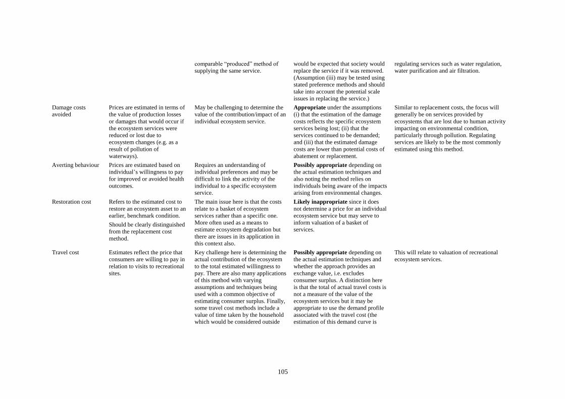
105

comparable “produced” method of

supplying the same service.

would be expected that society would

replace the service if it was removed.

(Assumption (iii) may be tested using

stated preference methods and should

take into account the potential scale

issues in replacing the service.)

regulating services such as water regulation,

water purification and air filtration.

Damage costs

avoided

Prices are estimated in terms of

the value of production losses

or damages that would occur if

the ecosystem services were

reduced or lost due to

ecosystem changes (e.g. as a

result of pollution of

waterways).

May be challenging to determine the

value of the contribution/impact of an

individual ecosystem service.

Appropriate under the assumptions

(i) that the estimation of the damage

costs reflects the specific ecosystem

services being lost; (ii) that the

services continued to be demanded;

and (iii) that the estimated damage

costs are lower than potential costs of

abatement or replacement.

Similar to replacement costs, the focus will

generally be on services provided by

ecosystems that are lost due to human activity

impacting on environmental condition,

particularly through pollution. Regulating

services are likely to be the most commonly

estimated using this method.

Averting behaviour Prices are estimated based on

individual’s willingness to pay

for improved or avoided health

outcomes.

Requires an understanding of

individual preferences and may be

difficult to link the activity of the

individual to a specific ecosystem

service.

Possibly appropriate depending on

the actual estimation techniques and

also noting the method relies on

individuals being aware of the impacts

arising from environmental changes.

Restoration cost Refers to the estimated cost to

restore an ecosystem asset to an

earlier, benchmark condition.

Should be clearly distinguished

from the replacement cost

method.

The main issue here is that the costs

relate to a basket of ecosystem

services rather than a specific one.

More often used as a means to

estimate ecosystem degradation but

there are issues in its application in

this context also.

Likely inappropriate since it does

not determine a price for an individual

ecosystem service but may serve to

inform valuation of a basket of

services.

Travel cost Estimates reflect the price that

consumers are willing to pay in

relation to visits to recreational

sites.

Key challenge here is determining the

actual contribution of the ecosystem

to the total estimated willingness to

pay. There are also many applications

of this method with varying

assumptions and techniques being

used with a common objective of

estimating consumer surplus. Finally,

some travel cost methods include a

value of time taken by the household

which would be considered outside

Possibly appropriate depending on

the actual estimation techniques and

whether the approach provides an

exchange value, i.e. excludes

consumer surplus. A distinction here

is that the total of actual travel costs is

not a measure of the value of the

ecosystem services but it may be

appropriate to use the demand profile

associated with the travel cost (the

estimation of this demand curve is

This will relate to valuation of recreational

ecosystem services.

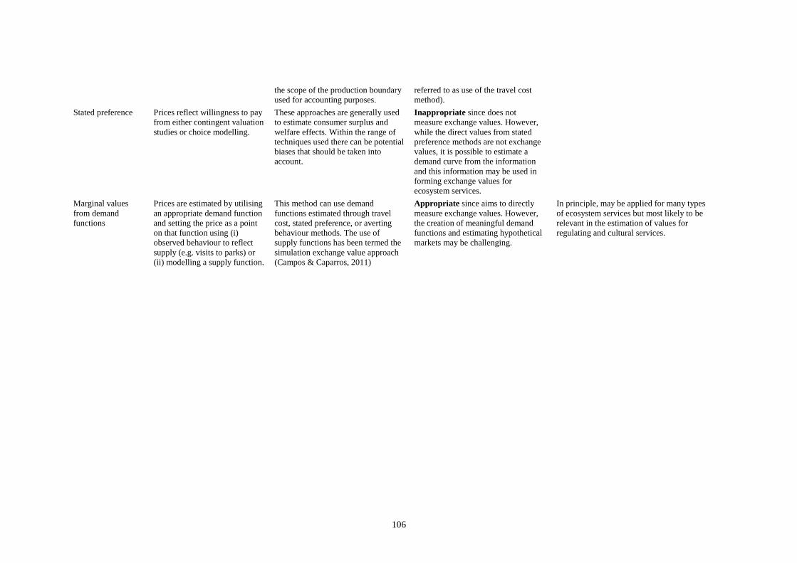
106

the scope of the production boundary

used for accounting purposes.

referred to as use of the travel cost

method).

Stated preference Prices reflect willingness to pay

from either contingent valuation

studies or choice modelling.

These approaches are generally used

to estimate consumer surplus and

welfare effects. Within the range of

techniques used there can be potential

biases that should be taken into

account.

Inappropriate since does not

measure exchange values. However,

while the direct values from stated

preference methods are not exchange

values, it is possible to estimate a

demand curve from the information

and this information may be used in

forming exchange values for

ecosystem services.

Marginal values

from demand

functions

Prices are estimated by utilising

an appropriate demand function

and setting the price as a point

on that function using (i)

observed behaviour to reflect

supply (e.g. visits to parks) or

(ii) modelling a supply function.

This method can use demand

functions estimated through travel

cost, stated preference, or averting

behaviour methods. The use of

supply functions has been termed the

simulation exchange value approach

(Campos & Caparros, 2011)

Appropriate since aims to directly

measure exchange values. However,

the creation of meaningful demand

functions and estimating hypothetical

markets may be challenging.

In principle, may be applied for many types

of ecosystem services but most likely to be

relevant in the estimation of values for

regulating and cultural services.

107

6.3.3 Alternatives to direct monetary valuation

6.35. The discussion in this chapter has a focus on the direct valuation of individual

ecosystem services. In some circumstances, complementary information concerning

economic activity associated with certain ecosystem services may provide a broader

picture of the economic relevance, or value, of these services.

6.36. For instance, governments may be interested in the resource rent generated by

different ecosystems under current management, but they may also be interested in, for

example, the net value added and employment that is generated in sectors dependent

upon services provided an ecosystem, as in the case of a fisheries or the nature-based

tourism sector. Since net value added indicates the return on the combined use of

ecosystem assets, produced assets and labour it provides a broader insight into the

economic significance of ecosystems compared to resource rent alone.

6.37. Furthermore, it is noted that measures of value added will be less affected by

the problem of zero rent in open access, common pool ecosystem resources, since in

such systems there will still be a return on labour and produced assets. Crucially, it also

provides a better measure of the relevance of ecosystem services in situations where

there are few alternative sources of income. For example, in the case where a significant

part of the population is involved in say fisheries or livestock raising, and where few

alternative employment options are available, the resource rent may severely

underestimate the economic significance of the resource for people in the area.

6.4 Key challenges and areas for research in valuation

6.38. There is a wide range of challenges in valuation. The following section

describes those that may be most commonly confronted beyond the issues already

raised in this chapter. Some of these will be particular targets for research work.

6.39. The target of valuation. In the SEEA EEA, the ecosystem accounting model

(see chapter 2) has a clear distinction between ecosystem services and the benefits to

which they contribute. Particularly for provisioning services, it is not uncommon for

the market price of the extracted good (e.g. fish caught or timber harvested) to be

considered equivalent to the value of the ecosystem service. In fact, the market price

reflects the value of the benefit and estimating the appropriate value for the associated

ecosystem service must involve deducting the costs of extraction and harvest, thus

leaving a residual that reflects the ecosystem contribution.

6.40. By way of example, in the case of timber harvest there will commonly be a

price for the logged timber – perhaps a roadside price. This price should be sufficient

to cover the costs of felling (labour, fuel, equipment, land management costs, etc.). It

should also cover any payments that are made to the owner of the forest for the right to

harvest the timber. These are commonly referred to as stumpage prices. The value of

the ecosystem services in this case is not the roadside price after felling, but the

stumpage price, equivalent to the residual after deducting the costs of extraction.

6.41. In some cases, this residual may be very small or negative (for example, in the

case of abstracted water or open access fishing). Consequently, the implied value of

the ecosystem service may very low, zero or negative from an exchange value

perspective. A number of different cases can be identified. For example, in the case of

water the resource rent is often near zero as there is commonly no competitive market

for distributed water and prices are regulated to only cover the costs of supplying water

to customers. In the case of open access fishing the lack of defined property rights is

the key driver for low values. In recreational hunting, the costs are often higher than

108

the potential sale price of the game meat but this will reflect the recreational value of

the activity.

6.42. Depending on the situation, different valuation approaches may be considered

as alternatives to resource rent techniques, for example using replacement costs in the

case of water or costs of hunting licenses in the case of recreational hunting (Remme

et al., 2014). Most problematic is determining an approach in the case of common pool

/ open access resources. Note that the benefits produced in these instances (e.g. fish or

water) still have market prices, but the ecosystem services are implicitly valued at near

zero, implying as well that ecosystem degradation would be valued at zero. Further

discussion on potential approaches for accounting in these situations would be

welcome.

6.43. Relating ecosystem assets to values for ecosystem services. An important

distinction is the one between the valuation of ecosystem services and the valuation of

ecosystem assets (and the related issue of valuing ecosystem degradation). Within

ecosystem accounting, the valuation of ecosystem assets reflects the overall value of a

given spatial area and is estimated by aggregating the net present value of all relevant

ecosystem services. These issues are discussed in Chapter 7.

6.44. In pricing theory, the capital costs associated with the supply of ecosystem

services, i.e. the cost of any ecosystem degradation, should influence the price set for

the outputs. Many approaches to valuation however, implicitly assume that the use of

the associated ecosystem asset is sustainable, thus setting these capital costs to zero.

The need to incorporate the effect of degradation on the prices of ecosystem services

is recognised as a challenge (see Bateman, et al. 2011) but it has not yet been resolved.

6.45. Valuation of subsistence production. In a number of situations, there may be

significant flows of ecosystem services associated with subsistence agriculture,

forestry and fisheries, i.e. where the growing and harvesting of the outputs from these

activities is not sold on markets but directly consumed by households. A broad range

of products may be relevant here including all types of non-timber forest products.

Following the conceptual scope of the SNA, the production associated with this activity

should be included in the national accounts estimates of output with exchange values

estimated on the basis of the prices of similar goods sold on markets. The handbook on

the measurement of the non-observed economy (OECD et al., 2002) provides guidance

on measurement approaches in this area. For ecosystem service valuation, the value of

the associated ecosystem services can be based on these estimated market prices using

techniques noted above for similar provisioning services such as unit resource rents

and production functions.

6.46. Valuation of intermediate services. The focus of valuation in the SEEA EEA,

and in the majority of other studies, is on final ecosystem services. This focus supports

understanding the interactions between ecosystem assets and users (i.e. economic units

including households). However, if the valuations of final ecosystem services are

attributed to specific ecosystem assets, it may imply that those ecosystem assets

supplying final ecosystem services have a particularly high value, relative to ecosystem

assets that do not supply final services directly. Thus, where there are important

dependencies between ecosystem assets in the supply of a final ecosystem service,

ignoring the value of intermediate services may provide misleading information on the

relative importance of certain ecosystem assets. At the same time, there are significant

measurement challenges and this area of measurement remains one for further research

and testing. More generally, the description and measurement of ecological production

functions would be an important pathway in understanding the connections between

ecosystems.

6.47. Valuation of regulating services. For most provisioning services, there is a

connection to market values of benefits that can provide a base for measurement. This

109

is also true for some – but by no means all - cultural services (such as those relating to

economic activity in tourism and recreation). However, in the area of regulating

services such connections to marketed benefits are unusual. Indeed, for regulating

services it can be difficult to appropriately define and measure the actual physical flow

of the service because often the service is simply part of ongoing ecosystem processes

rather than a function of direct human activity – for example, air filtration and carbon

sequestration. The challenge of valuation may thus lie primarily in articulating the link

between the services and human activity such that the application of valuation

techniques can be well-founded.

6.48. The measurement of non-use values. An important part of the value of

ecosystems from a societal perspective can lie in the non-use values that, in principle,

are captured in various cultural services provided by ecosystem assets. These values

include existence values (based on the utility derived from knowing that an ecosystem

exists); altruistic values (based on the utility derived from knowing that someone else

is benefiting from the ecosystem) and bequest values (based on the utility derived from

knowing that the ecosystem may be used by future generations). At this point, there are

relatively few studies in this area of valuation from the perspective of ecosystem

services although the discussion of this area of valuation is a particular focus within

the IPBES program of work (ref#). From an ecosystem accounting perspective, there

is a further open question of the extent to which non-use values can be captured using

an exchange value concept even if the associated ecosystem services may be

considered within scope.

6.49. The valuation of ecosystem assets with respect to land. In estimating the value

of ecosystem assets at exchange values, one important consideration is the value of

land that is commonly traded in markets – including, for example, agricultural land.

Depending on the circumstance, values of land will incorporate the value of some

ecosystem services. However, they are unlikely to capture the value of all of the

ecosystem services particularly those that are of a public good nature. Further, market

based land values will incorporate elements of value that are not dependent on

ecosystems, such as the prospects for property development or the capitalisation of

farm subsidies. Consequently, when considering the integration of ecosystem asset

valuations into existing national accounts balance sheets, some adjustments will be

required to ensure there is no double counting or gaps in valuation for the estimation

of total net wealth.

6.50. The valuation of biodiversity and resilience. Biodiversity and resilience are

considered in SEEA EEA primarily as characteristics of ecosystem assets and not as

ecosystem services. Consequently, they are not separately valued using the general

approach outlined here and the relative contribution of biodiversity and resilience is

unlikely to be identifiable. Further consideration on how these aspects of ecosystem

assets may be incorporated into valuations is required, including in terms of how these

characteristics feature in the description of ecological production functions.

6.51. Channels of ecosystem services. Underlying many of these challenges in

valuation have been differences of view in the conception of value and its application.

As noted earlier, one source of this difference has been the different perspectives of

non-market valuation from accountants and economists. Through the ongoing World

Bank valuation research seeking to better understand and bridge these differences, a

potential way forward has emerged after identifying a valuation framing widely

understood in environmental economics but not known to accountants. This framing

considers valuation in terms of different channels between the environment and

business, individuals and society. Freeman (2013) identifies three main channels:

110

inputs to production, inputs to household consumption28 and inputs to well-being29. In

short:

• Channel #1 – Inputs to production: These are ecosystem services that are used as

inputs to economic production. Among many examples these include water

regulation and water purification services which are inputs to those economic

(producing) units which need a supply of clean water as an input alongside other

factors of production. Importantly, this channel is not limited to the valuation of

provisioning services since a range of regulating and cultural services will provide

inputs to production.

• Channel #2 – Inputs to household consumption: These are ecosystem services that

can act as joint inputs to household consumption. 30 That is, there is use of

ecosystem services in combination with (or as a substitute for) expenditure on

produced goods and services in providing a “product” for consumption. In such

cases, ecosystem services and the market goods/services are complementary (or

substitute) inputs, and because of this, expenditure on the latter provides a guide to

the value placed on the former. Examples include the contribution of ecosystems

to recreation and tourism, which are combined with human inputs (e.g. in the form

of hotels, restaurants, walking paths) to produce recreation benefits. An example

where an ecosystem service is a substitute for market expenditure is air purification

services which can substitute for the purchase of a produced good which filters the

air.31

• Channel #3 – Inputs to well-being: These are ecosystem services that can be inputs

which directly contribute to household wellbeing. That is, there is no existing

economic production or household consumption where these services first act as

inputs. These services are consumed directly in generating benefits: that is, directly

from nature without any other (produced) inputs. Examples here are, by their

nature, rather abstract and less tangible, but include those services which are valued

for reasons of what is usually termed ‘non-use’ or ‘passive-use’.

6.52. All of these channels are well understood in the environmental economic

literature on categorizing ecosystem services for valuation purposes. As distinct from

an externality based framing for valuation as commonly applied in environmental

economics, this “channels” based approach seems to provide a much more direct

parallel to the way in which national accountants seek to frame the valuation question.

Indeed, the different channels can be seen as equivalent conceptually to different cells

within a supply and use account which each record a distinct link between supplier (in

this case the ecosystem asset) and user (in this case the different economic units).

6.53. The key conclusion that is emerging from this line of thinking is that the choice

of valuation technique will not be purely dependent on the type of ecosystem service –

which has been the most observed approach to date. In addition, the choice of valuation

technique must also consider the characteristics of the user. In many cases this may not

28 Strictly speaking, this channel is often referred to as household production. That is, the production of

output consumed by a given household, through a combination of inputs from ecosystem services and

expenditure on a market good (or goods). 29 That is, the flow of some ecosystem service contributes directly to household wellbeing rather than via its

contribution to economic production or household consumption. 30 Typically, in environmental economics this is referred to as “household production” We refer to

“consumption” here as it is the conventional terminology in accounting. 31 Firms may also undertake these sort of defensive expenditures: that is, purchase substitute goods to defend

against an environmental burden, which exists in the absence of some ecosystem service. The value of this

service then might be approximated by estimating how the cost of producing current output changes as a

result of a small change in its provisions. Given that this refers to the production side of the economy, this

is a pathway under Channel #1 rather than Channel #2, which is defined here as referring to household

consumption.

111

make a significant difference to the choices that have been made, but it does provide a

valuation context that is more satisfactory from a national accounting perspective.

6.54. The research into the use of framing valuation in terms of channels is ongoing

and at this stage cannot be elaborated further in these Technical Recommendations. It

is noted here to encourage ecosystem accounting compilers to continue to engage with

the environmental economics valuation community to find means by which the

challenge of valuation of ecosystem services can be advanced.

6.5 Recommendations on the valuation of ecosystem services

6.55. There remains a substantial amount of work to be conducted to advance

valuation in the context of ecosystem accounting. At one level, there is a need to

continue the discussion about the role of valuation both in general terms and with

respect to accounting. The main challenge is to provide the appropriate context for the

discussion since commonly there are many misunderstandings of the relevant issues.

A key issue is understanding that there are different purposes for valuation and there

may be some questions that are not best considered using information in monetary

terms.

6.56. At a second level, there is a need for understanding and explaining the concept

of exchange values for accounting purposes and the development, or adjustment of,

valuation techniques to support the estimation of this valuation concept. A possible

path forward on this is to distinguish better between the relevant valuation techniques

as to: (i) when the ecosystem services can be relatively easily linked to existing market

prices and (ii) when the ecosystem services relate to public goods. These two principal

targets for valuation involve different challenges.

6.57. One of the most important challenges in accounting is to ensure that the users

of the accounts understand the valuation concepts applied in the accounts. Specifically,

they should understand that the accounts do not provide an estimate of ‘the value of

nature’ or even ‘the economic value of ecosystems’. Instead, the monetary ecosystem

accounts estimate the monetary value of the contribution of ecosystems to economic

production and consumption – at least to the extent that a comprehensive set of

ecosystem services has been used and valuation of these services is possible.

6.58. Where ecosystem services can be relatively easily linked to market prices (e.g.

provisioning services and tourism related services), an important part of the

information required for valuing the service may already be in the national accounts.

For these services, valuation serves to specify the contribution of the ecosystem to the

related benefits already included in the national accounts in monetary terms. Following

Table 8.1, for such services a resource rent-based valuation approach may be

appropriate, noting potential challenges described above concerning the estimation of

low or negative resource rents. The SNA (EC et al, 2009) and the OECD Measuring

Capital manual (OECD, 2009) provide detailed guidance on how intermediate inputs,

labour and fixed capital should be costed, including for example estimation of rates of

return to produced assets.

6.59. The SEEA EEA approach involves the combination of tabular and mapped

information. Producing maps for ecosystem services that are valued based on

information that is in the national accounts generally involves spatial allocation. In

some cases, this is straightforward, as in the case of forests providing timber to a

logging company. In other cases, some modelling of spatial interactions between

ecosystem users and the ecosystem asset is required, as in the case of allocating the

resource rent generated in the tourism sector to (natural) ecosystems.

112

6.60. In the case of public services, including most regulating services that are not

captured in the national accounts, spatial models for the physical flows of ecosystem

services involved provide the basis for valuation. Significant uncertainty may pertain

to both the physical models (as discussed in Chapter 5) and the unit values for the

ecosystem services. Different regulating services require different valuation methods.

Replacement costs methods can be applied, based on the least-cost alternative, if it can

reasonably be assumed that the service would indeed be replaced if lost. This method

is relevant, for instance, for the flood protection service of coastal or riparian

ecosystems in densely populated areas. In case it cannot be assumed that the service

would be replaced, an avoided damage cost method may be appropriate (see Table 8.1).

Hedonic pricing is another valuation method with which there is ample experience. It

can be used to value for example the cultural service underpinning the positive amenity

that people obtain from nature, as in the case of eliciting the incremental value of

houses with a view or close to green space.

6.61. Other valuation methods have as yet been less frequently applied, but offer the

potential to broaden the pallet of valuation methods available for SEEA EEA. For

instance, the Simulated Exchange Value approach and the Travel Cost Method can be

used to reveal demand curves which would allow a more comprehensive inclusion of

tourism and recreation in the ecosystem accounts. Well-functioning Payment Schemes

for Ecosystem Services may indicate partial market equilibrium demand and supply

for ecosystem services, and associated market prices, but it needs to be examined under

what conditions the prices paid for ecosystem services in a PES truly reflect exchange

values.

6.62. In general, there is a need for further efforts to estimate exchange values of

ecosystem services in practice, for a basket of ecosystem services, across a range of

ecosystem types. There are some examples of work heading in this direction (see for

example Remme et al., 2014; Sumarga and Hein, 2014) but more testing is required.

For some techniques (hedonic pricing, replacement costs, avoided damage costs) there

is ample experience in the environmental economics literature that can be built upon.

in other cases, e.g. simulated exchange values and the use of the travel cost method and

prices from PES schemes in the context of accounting, there is a need for further

research before such valuation approaches can become more standardized.

113

7 Accounting for the value and capacity of ecosystem assets

Key points in this chapter

The ecosystem monetary asset account records the monetary value of the opening and closing stocks of

all ecosystem assets within an ecosystem accounting area and additions and reductions in those stocks.

Estimates of the monetary value of ecosystems are compiled using the exchange value concepts

developed in Chapter 6. This facilitates integration with the values of other assets such as buildings,

machinery and equipment, and financial assets.

In most cases, monetary values of assets are estimated based on the net present value (NPV) of the

expected future flows of all ecosystem services generated by an ecosystem asset. This requires an

understanding of the likely pattern for the supply and use of each ecosystem service and recognition that

the pattern of supply among different ecosystem services from a single ecosystem asset is likely to be

correlated.

The estimation of net present value also requires the selection of a discount rate and this choice can have

an important impact on the resulting valuations.

A key aspect in understanding the pattern of future flows of ecosystem services is the connection to the

condition of the ecosystem asset. This connection between services and condition is reflected in the

concept of ecosystem capacity. Ecosystem capacity can be measured in both physical and monetary

terms.

The measurement of ecosystem capacity also links to the measurement of ecosystem degradation, i.e. the

decline in the condition of ecosystem assets as a result of economic and other human activity.

Further testing and research is required in many areas related to measuring the monetary value and

capacity of ecosystem assets including the application of NPV techniques for ecosystem assets,

estimating future patterns of ecosystem service flows, the measurement of ecosystem capacity and the

valuation and attribution of ecosystem degradation.

7.1 Introduction

7.1. The discussion of accounting for the monetary value and capacity of ecosystem

assets in this chapter, and the associated discussion of integration with economic

accounts in Chapter 8, is directly linked to the way in which national accountants make

the connection to ecosystem information. It is also directly related to the literature on

wealth accounting (UNU-IHDP and UNEP, 2014; Hamilton and Clemens, 1999) as it

concerns the valuation of natural capital. Given this perspective, some initiatives in

ecosystem accounting see that accounting for ecosystem assets in monetary terms is

the underlying rationale for measurement in this area (see for example accounting work

in the context of the English Natural Capital Committee). The discussion in the SEEA

EEA and in these Technical Recommendations is designed to recognise this is not the

only perspective that can be taken.

7.2. Underpinning accounting for ecosystem assets in monetary terms is the idea

that the monetary value of ecosystem assets can be estimated in the same way as for

other assets, i.e. in terms of the future flow of income attributable to an asset.

Conceptually, this is true for the value of all economic assets. For most economic

assets, this value is estimated for SNA purposes on the basis of recording actual

transactions in assets (e.g. the sale and purchase of buildings and equipment). Where

the markets for specific assets are thin or do not exist, such as occurs for ecosystem

assets, the SNA proposes alternative valuation techniques including the use of the

discounted flows of future income (see SEEA EEA Section 5.4 for a summary). This

chapter discusses the approaches and challenges in undertaking this aspect of

ecosystem accounting.

114

7.3. The standard logic for accounting for ecosystem assets in monetary terms is to

(i) identify the basket of ecosystem services that an ecosystem asset supplies, (ii)

estimate the expected ecosystem service flows, i.e. the flows of each type of ecosystem

service that are considered most likely to occur based on current expectations of the

use of the ecosystem, (iii) apply appropriate prices to each flow of ecosystem services

and discount each flow to the current time period. This discounted value of future flows

represents the net present value of ecosystem assets. This approach follows standard

capital accounting theory (see OECD, 2009), and recognises a direct connection

between the valuation of ecosystem services and ecosystem assets.

7.4. The expected ecosystem service flows (a concept introduced in SEEA EEA,

para 2.40) may be higher or lower than the level of ecosystem flows that might be

considered sustainable. That is, the estimation of ecosystem asset values at any point

in time should not assume sustainable use. To do this would imply that ecosystem

assets cannot be the subject of ecosystem degradation. At the same time, it may be of

considerable interest to understand the difference between expected ecosystem service

flows and the level of flows that would be sustainable, i.e. the level that would imply

no loss in ecosystem condition in the future. This links directly to the concept of

ecosystem capacity. Given the importance of these topics, this chapter discusses at

some length the concepts and measurement of ecosystem capacity and ecosystem

degradation, with a general conclusion that more discussion and investigation is

required to reach a more common understanding of these issues.

7.2 Ecosystem monetary asset account

7.2.1 Description of the account

7.5. The ecosystem monetary asset account records the monetary value of opening

and closing stocks of all ecosystem assets within an ecosystem accounting area and

additions and reductions in those stocks. Estimates of ecosystem assets in monetary

terms are useful for making decisions about alternative uses of ecosystem assets since

they provide a consistent basis for comparison. In addition, estimates in monetary terms

can be integrated with valuations for other types of assets to provide more complete

assessments of net wealth. A decline in value of ecosystem assets at aggregated scales

(e.g. in the EAA) may point to unsustainable ecosystem use.

7.6. The relevant accounting structure for the ecosystem monetary asset account is

shown in Table 7.1. The entries in the rows have been simplified to very basic asset

account entries. If more detail is required to account for changes in assets, particularly

those related to provisioning services, then additional entries following the structure of

the monetary asset account in the SEEA Central Framework (Table 5.3) can be

incorporated. These additional entries include growth and normal losses of stock,

catastrophic losses (e.g. changes due to natural disasters), upward and downward

reappraisals and reclassifications. A separate entry is used to record changes between

the opening and closing values of ecosystem assets that are due to revaluations – i.e.

changes in the value that are due solely to changes in prices rather than changes in

volumes.32

7.7. In the columns, different presentations are possible given that the data are in

monetary terms. That is, an asset account can be scoped and structured to refer to an

individual ecosystem asset (e.g. a specific grassland), to a specific ecosystem type (e.g.

all tree-covered areas), or to an ecosystem accounting area (as shown below).

32 Note that following SEEA Central Framework 5.61, a change in the quality of an ecosystem asset, e.g.

due to a change in condition, is considered a change in volume rather than a revaluation.

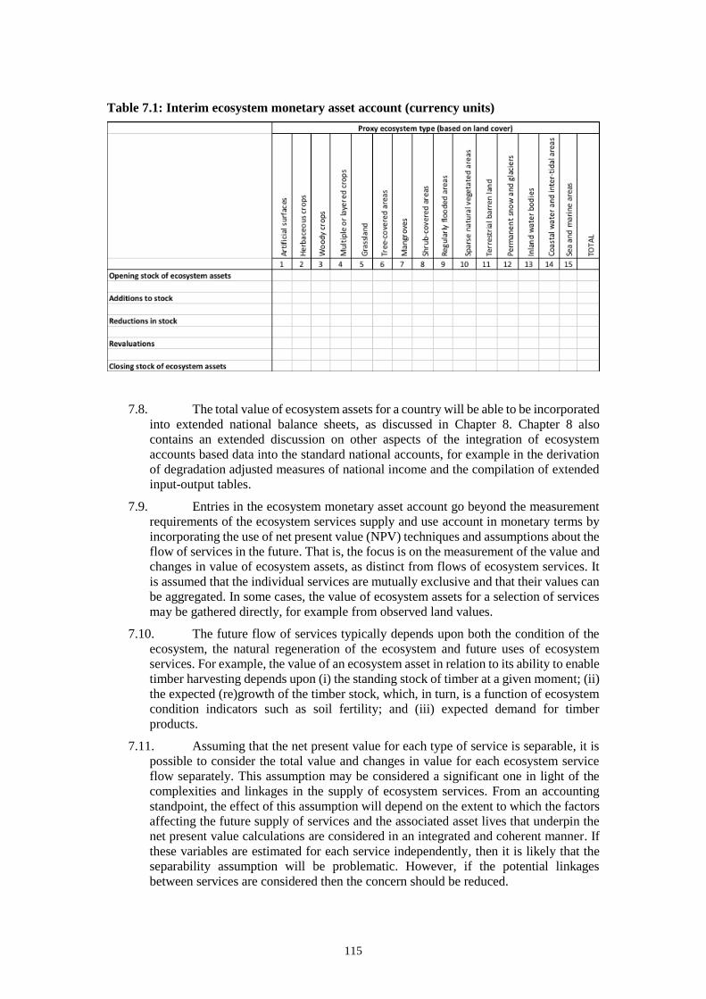
115

Table 7.1: Interim ecosystem monetary asset account (currency units)

7.8. The total value of ecosystem assets for a country will be able to be incorporated

into extended national balance sheets, as discussed in Chapter 8. Chapter 8 also

contains an extended discussion on other aspects of the integration of ecosystem

accounts based data into the standard national accounts, for example in the derivation

of degradation adjusted measures of national income and the compilation of extended

input-output tables.

7.9. Entries in the ecosystem monetary asset account go beyond the measurement

requirements of the ecosystem services supply and use account in monetary terms by

incorporating the use of net present value (NPV) techniques and assumptions about the

flow of services in the future. That is, the focus is on the measurement of the value and

changes in value of ecosystem assets, as distinct from flows of ecosystem services. It

is assumed that the individual services are mutually exclusive and that their values can

be aggregated. In some cases, the value of ecosystem assets for a selection of services

may be gathered directly, for example from observed land values.

7.10. The future flow of services typically depends upon both the condition of the

ecosystem, the natural regeneration of the ecosystem and future uses of ecosystem

services. For example, the value of an ecosystem asset in relation to its ability to enable

timber harvesting depends upon (i) the standing stock of timber at a given moment; (ii)

the expected (re)growth of the timber stock, which, in turn, is a function of ecosystem

condition indicators such as soil fertility; and (iii) expected demand for timber

products.

7.11. Assuming that the net present value for each type of service is separable, it is

possible to consider the total value and changes in value for each ecosystem service

flow separately. This assumption may be considered a significant one in light of the

complexities and linkages in the supply of ecosystem services. From an accounting

standpoint, the effect of this assumption will depend on the extent to which the factors

affecting the future supply of services and the associated asset lives that underpin the

net present value calculations are considered in an integrated and coherent manner. If

these variables are estimated for each service independently, then it is likely that the

separability assumption will be problematic. However, if the potential linkages

between services are considered then the concern should be reduced.

116

7.12. For example, if estimates of carbon sequestration services are made assuming

that a forest can sequester carbon over an infinite timeframe, while for the same

ecosystem asset, estimated rates of timber provisioning are made assuming the forest

is depleted within a limited time frame with no regeneration (e.g. 30 years), then the

two estimates of expected service flows should be considered internally inconsistent.

In many cases, it is likely that asset lives for provisioning services involving harvest or

extraction will provide an upper bound to the asset lives and should therefore be applied

in estimation of all expected ecosystem service flows.

7.13. For provisioning services, such as timber extraction, accounting for the

additions and reductions is conceptually straightforward. In this case, the value of

provisioning services will reflect a resource rent (taking into account the estimation

challenges noted in Chapter 6). Therefore, accounting for the changing value of

provisioning services is equivalent to the advice provided in the SEEA Central

Framework and the SNA on accounting for individual environmental assets. Applying

this approach is possible since the underlying physical flows (e.g. of timber resources)

can be accounted for using a single metric.

7.14. For regulating and cultural services, the link to underlying physical flows may

be less clear. For regulating services, the issue is that the supply of the service does not

only depend upon the extent and condition of the ecosystem, but also upon other factors

that will not be stable over time. For example, air filtration is a function of the extent

and type of vegetation and its leaf area index, but it is also influenced by expected air

pollution levels and these can be spatially and temporally heterogeneous. Thus, the

higher the concentration of atmospheric particulate matter, the higher the amount of

particulate matter that is normally captured by the vegetation.

7.15. In addition, most regulating services depend upon a variety of ecosystem

characteristics and processes, with each of them providing only limited information on

the capacity of the ecosystem to supply the service over time. Relevant indicators may

therefore reflect ecosystem characteristics, such as leaf area index per BSU in the case

of air filtration, or they may reflect outputs of the ecosystem, for instance, the amount

of water made available for irrigation throughout the year in the case of the water

regulating service provided by forests. Establishing accounting entries for changes in

ecosystem asset values related to regulating services is therefore not straightforward.

7.16. For cultural services, it may also be challenging to find appropriate physical

data for quantifying the services in terms of the underlying ecosystem assets. Cultural

services can involve a passive interaction (enjoying without visiting through

information obtained from various media) or active interaction (actual visitation) with

an ecosystem. Thus, describing the link between the condition of the ecosystem in

physical terms and the supply of cultural services may be difficult to define in general

terms. For example, in the case of recreation, a natural park may physically allow

access to a large number of people, but, at some point, the recreational experience

gained per individual will decline because of overcrowding.

7.17. Overall, policy-relevant physical indicators about ecosystem assets can be

defined for most provisioning services, while indicators for regulating services are

more complicated to define but are an active area of research and testing. Indicators for

cultural services require the most further development at this stage. It will be

appropriate to consider the selection and measurement of these indicators in

combination with the development of indicators of condition.

7.18. In a fully spatial approach where sufficient data are available, it is possible to

map ecosystem asset values and, where time series are available, identify areas subject

to declines in the value of ecosystem assets.

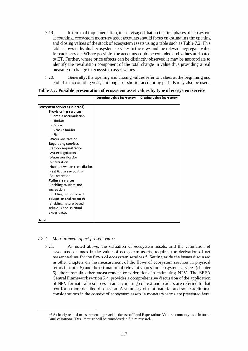
117

7.19. In terms of implementation, it is envisaged that, in the first phases of ecosystem

accounting, ecosystem monetary asset accounts should focus on estimating the opening

and closing values of the stock of ecosystem assets using a table such as Table 7.2. This

table shows individual ecosystem services in the rows and the relevant aggregate value

for each service. Where possible, the accounts could be extended and values attributed

to ET. Further, where price effects can be distinctly observed it may be appropriate to

identify the revaluation component of the total change in value thus providing a real

measure of change in ecosystem asset values.

7.20. Generally, the opening and closing values refer to values at the beginning and

end of an accounting year, but longer or shorter accounting periods may also be used.

Table 7.2: Possible presentation of ecosystem asset values by type of ecosystem service

7.2.2 Measurement of net present value

7.21. As noted above, the valuation of ecosystem assets, and the estimation of

associated changes in the value of ecosystem assets, requires the derivation of net

present values for the flows of ecosystem services.33 Setting aside the issues discussed

in other chapters on the measurement of the flows of ecosystem services in physical

terms (chapter 5) and the estimation of relevant values for ecosystem services (chapter

6); there remain other measurement considerations in estimating NPV. The SEEA

Central Framework section 5.4, provides a comprehensive discussion of the application

of NPV for natural resources in an accounting context and readers are referred to that

text for a more detailed discussion. A summary of that material and some additional

considerations in the context of ecosystem assets in monetary terms are presented here.

33 A closely related measurement approach is the use of Land Expectations Values commonly used in forest

land valuations. This literature will be considered in future research.

118

7.22. First, it is necessary to understand the expected asset life of the ecosystem.

That is, an understanding is required of the length of time that ecosystem services will

be supplied into the future. As noted above, this should not be done independently for

each ecosystem service. In many cases, the supply of regulating and cultural services

will be competing relative to the supply of provisioning services. In these

circumstances, it is likely that the estimated asset life for provisioning services provides

the relevant upper bound for the asset life assumption. Where an ecosystem asset is

being used sustainably, i.e. with no expected decline in ecosystem condition, the asset

life appropriate at the current estimation date will be infinite. The estimation of asset

lives is directly related to the discussion of ecosystem capacity and ecosystem

degradation presented in sections 7.3 and 7.4.

7.23. In the derivation of macro-level estimates of national wealth, it is common for

a generic asset life to be assumed (e.g. 25 years) rather than estimating asset lives that

take into account the balance of ecosystem condition and expected service flows. (See

for example World Bank, 2011.) Clearly this is more straightforward methodologically.

It may also be rationalised at an aggregate level since where discount rates of greater

than 5% are used, the contribution of future income flows beyond 30 years to the total

asset value diminishes to around 20% (at 5% discount rates) and to around 6% (at 10%

discount rates) (See Table A5.1 in SEEA Central Framework Annex A5.2). That is, at

higher discount rates much of the value of ecosystem assets will be captured in the first

25-30 years. However, since there is a strong correlation between the choice of asset

life and the choice of discount rate, if a generic asset life is assumed then compilers are

encouraged to undertake estimation for a variety of asset life and discount rate

alternatives to assess and convey the sensitivity of ecosystem asset values to these

choices.

7.24. A priori, there is no preferable generic asset life since it will depend on the

condition of the ecosystem asset and the expected patterns of use. Therefore, as far as

possible within available resources, it is recommended that investigation be undertaken

into specific asset lives, at least for different ecosystem types. Such work will provide

a more robust estimate of the asset lives, and the process will also serve as a form of

data confrontation in terms of expectations concerning the supply of various ecosystem

services and the potential changes in condition, taking into account various driving

forces, for example population growth.

7.25. Second, the derivation of NPV requires describing the expected future flows

of ecosystem services. This flow may be affected by many considerations, in particular

ecosystem condition. It may be useful to separately consider future flows in physical

terms and future changes in values of those ecosystem services. A common assumption

in national accounting for natural resources is to assume that the resource rent per tonne

extracted (unit resource rent) stays constant over the remaining asset life. However,

this should only be considered a default basis for estimation, and it would be

considerably better if an assessment of possible future trade-offs between different

services was undertaken.

7.26. Keeping in mind that the ambition is to provide the best estimate of expected

flows, even when assuming the unit resource rent (or more broadly the value per unit

of ecosystem services) stays constant into the future, it is possible that the past time

series of unit resource rents shows a degree of volatility. In such cases it is

recommended that an average of recent periods (say 3-5 years) is used as the basis for

estimating future flows. Note that where changes in unit resource rent occur that may

be attributed to structural change (e.g. due to changed regulations) then averaging over

time periods may not be appropriate. Generally, it should be clear that the requirement

to use expectations to determine asset values means these values are less reliable. It is

also observed, that the framing for establishing values based on expectations can also

119

be applied to establish values based on alternative future scenarios (i.e. scenarios that

may not be the most likely).

7.27. The use of bio-economic models may be of particular relevance in estimating

asset lives. These models take into account ecological dynamics and spatial scale in

evaluating the stocks of natural resources, e.g. fish stocks, and may provide significant

insight into the likely future patterns of ecosystem services and changes in underlying

ecosystem assets. Recent research by Fenichel and Abbot (e.g. 2014) has been

investigating the valuation of ecosystem assets taking these ecological dynamics into

account within the framework of standard capital accounting theory. This work

provides some important insights for use in the valuation of ecosystem assets in an

ecosystem accounting context.

7.28. Third, as mentioned above, a discount rate is required. The choice of discount

rate is an area of much discussion. Economists are by no means clear on what discount

rates might be appropriate and there are a number of factors to take into consideration.

SEEA Central Framework Annex A5.2 provides a useful summary but also highlights

the lack of clarity in advice from experts in this area. Perhaps the key issue for

ecosystem accounting is clearly articulating the purpose of valuation and hence the

intended valuation concept. Where integration with existing national accounts

estimates of income and assets is required, then an exchange value concept is

appropriate. Consistent with this choice, the use of a market based discount rate is then

appropriate.

7.29. However, where a societal based valuation is required, then other

considerations are relevant, in particular assumptions about the relative social

importance of different ecosystem services. There may also be interest in identifying

the extent to which certain aspects of ecosystem are substitutable along the lines of

defining critical natural capital (Ekins, 2003). Where preferences or desired outcomes,

including taking into account the preferences of future generations, are introduced in

the determination of discount rates, as distinct from the market based approach which

has a focus on expected flows, the task of selecting a discount rate likely moves outside

of the remit of a national statistical office. That said, it must be accepted that there is

an underpinning set of assumptions and norms that are implicit in a decision to use

market based discount rates.

7.30. Given the range of different discount rates that may be chosen and the impact

that the choice can have on estimates of ecosystem asset value, compilers are

encouraged to undertake estimation for a variety of discount rates to demonstrate the

sensitivity of the estimates.

7.31. There is an important link between the choice of approach to estimating future

flows of ecosystem services and the choice of discount rate. Where it is assumed that

the unit values of ecosystem services will remain constant over the asset life, it is

necessary to use a discount rate in real terms, i.e. after adjusting for inflation.

Conversely, where the future path of ecosystem services unit values is directly

estimated and included in the calculations, then a nominal discount rate should be used.

When adjusting a discount rate for inflation (i.e. converting it to real terms), since the

essence of a discount rate is to reflect the time value of money, an appropriate measure

of inflation is likely one that is economy wide in scope, such as the GDP deflator.

7.32. Fourth, in the estimation of net present values it is usual for a number of past

years to be compiled at the same time to provide a time series. However, each NPV

calculation for a specific time point must be based on the expectations relevant at that

time point. Thus, for example, where regulations change such that the use of an

ecosystem asset changes, estimates of NPV prior to the change should be based on the

earlier set of regulations and should not be revised on the basis of the changed situation.

The change in value associated with the change in circumstance (e.g. regulation

120

change) should be recorded as an addition or reduction in the value of ecosystem assets

during the relevant accounting period.

7.3 Measuring ecosystem capacity

7.3.1 Defining ecosystem capacity

7.33. The SEEA EEA describes three main ecosystem asset concepts: ecosystem

extent, ecosystem condition and expected ecosystem service flows. Ecosystem capacity

was recognised to be central to making the connection between ecosystem assets and

ecosystem services in accounting terms, but the nature of this connection was not

articulated in SEEA EEA. This was for two reasons:

• First, there was recognition that the link between ecosystem assets and

ecosystem services is hard to define and measure in ecological terms,

particularly in terms of the link between changes in overall ecosystem

condition and the supply of individual ecosystem services. Notions of

threshold effects, resilience, ecosystem dynamics and other non-linear factors

are important to consider.

• Second, since the concept of ecosystem capacity was considered to relate to

the overall ecosystem asset, a requirement in measuring capacity was defining

an expected basket of ecosystem services. Discussion on how such a basket

should be defined was not conclusive.

7.34. Since the release of SEEA EEA in 2013, it has become increasingly apparent

that the concept of ecosystem capacity is a central one for explaining the ecosystem

accounting model and applying the model in practice. This is especially the case in

relation to developing information sets that can support the discussion of sustainability.

It is thus clear that further research to capture the key aspects of ecosystem capacity

and how they interrelate is needed, together with practical examples. This section

provides an initial discussion of this topic utilising material from recent research in

Hein et al. (2016).

7.35. An initial definition of ecosystem capacity for accounting purposes is – the

ability of an ecosystem to generate an ecosystem service under current ecosystem

conditions and uses at the maximum yield or use level that does not negatively affect

the future supply of the same or other ecosystem services (Hein et al., 2016).

7.36. In the context of developing this definition, the following key points have

emerged. A longer discussion of the relevant issues is provided in Hein et al. (2016).

That paper also discusses issues in applying the concept of capacity to the different

types of ecosystem services, i.e. provisioning, regulating and cultural services and a

number of real-world examples are provided in which capacity is assessed. It is noted

that ecosystem capacity is being discussed in this later chapter of the Technical

Recommendations because it involves the joint discussion of ecosystem condition and

ecosystem services and measurement, noting that its measurement is relevant in both

biophysical and monetary terms.

7.37. Key recent insights concerning ecosystem capacity are:

i. First, capacity needs to be analysed for specific ecosystem services. The

capacity of a forest to supply wood will be different from its capacity to capture

air pollutants or sequester carbon. Capacity will have a different connotation

for the three types of services provisioning, regulating and cultural.

ii. Second, there is a temporal dimension to the analysis of capacity. Whereas the

harvest or use of provisioning services generally occurs at specific moments in

121

time, regeneration of ecosystems is a continuous process. In other words,

measures of capacity must reflect the stock of ecosystem assets and its ability

to supply individual services as a flow over time. In general terms, capacity

involves estimating the sustainable use level of ecosystems, in the sense that

there is sufficient regeneration (growth less natural losses) of the ecosystem to

offset the use of the ecosystem by economic units.

iii. Third, using one ecosystem service can reduce the ecosystem’s capacity to

supply other ecosystem services. For instance, harvesting wood may reduce

opportunities for nature-based tourism in a forest. Capacity, therefore, needs

to be assessed in the context of the actual use of the ecosystem, e.g. by

considering the carbon sequestration of a forest in the context of actual rates

of timber harvesting in a forest. It will also be relevant to consider competing

uses of ecosystems when considering the future flows of ecosystem services.

iv. Fourth, capacity is a measure that should relate to both the supply and use of

ecosystem services. Analysing capacity therefore requires understanding

demand for the services that an ecosystem asset generates. If there is no

demand for a service, the ability of an ecosystem to generate that service is not

relevant for assessing ecosystem capacity. This could be the case, for example,

for a flood control service provided in an area without people. Hence, capacity

is akin to sustainable use levels conditional on there being a demand for the

services involved.

v. Fifth, the definition of capacity is generally appropriate at more aggregated

scales, in particular at the landscape scale and above. If capacity is assessed

over too small an area, signals regarding changes in capacity may be

misleading because natural fluctuations or ecosystem use will more strongly

influence the ecosystem’s state relative to when larger areas are assessed (Hein

et al., 2016). For example, timber harvesting generally takes place in rotation

periods, and the capacity to generate timber would logically be assessed for a

complete forest asset rather than for individual stands.

7.38. For ecosystem accounting, capacity is related to the actual basket of ecosystem

services supplied. Thus, capacity requires the presence of users of ecosystem services.

Capacity therefore differs from the ability of an ecosystem asset to supply ecosystem

services independently from the potential use of those services by beneficiaries. This

has been labelled potential ecosystem service supply (e.g. Bagstad et al., 2014; Hein et

al., 2016). It may also differ from the basket of ecosystem services that would be

obtained under optimal ecosystem management, which could be labelled ‘the capability

of an ecosystem to supply services’ (Hein et al., 2016). Both potential supply and

capability are relevant concepts for ecosystem management but would not necessarily

underpin ecosystem accounting estimates (although they may be derived from a

common underlying information set covering, for example, measures of extent and

condition).

7.39. In cases where high levels of use of the ecosystem asset take place, e.g. through

high levels of extraction, it is expected that the actual flows of ecosystem services will

be higher than the sustainable flow and hence the condition of the asset will fall. This

set of circumstances would reflect ecosystem degradation.

7.40. Considering the above, capacity may be monetised on the basis of the NPV of

the sustainable flow of ecosystem services. A choice may need to be made in case there

are trade-offs between services. For example, sustainable timber logging may not

compatible with providing maximum recreational opportunities or air filtration

services from the ecosystem. For accounting purposes, the basis for this choice should

be the actual or revealed patterns of use and any associated legal and institutional

arrangements. Thus, if the forest is currently used primarily for timber logging, then

122

sustainable timber logging rates should be calculated and estimates for other ecosystem

services (e.g. air filtration, recreation) should be made with the same logging rates in

mind, rather than estimating capacity for each service based on alternative patterns of

use. At the same time, more consideration is required as to how this may apply in

practice. One consideration for example, may be that the unit values of ecosystem

services estimated with respect to actual use are not equivalent to those that would

apply in the context of sustainable use.

7.41. Even without this consideration, note that the NPV of ecosystem use at

capacity may be lower than, higher than or equal to the NPV of actual use of the

ecosystem. The selected discount rate and discounting period will have a major

influence on the different valuations.

7.42. Considering capacity as being measurable in terms of individual ecosystem

services is an important step forward in an accounting context, since it permits a direct

link to discussions of sustainable yield and flow that are well established in biological

models and resource economics. However, there remain significant challenges in

understanding the links between measures of capacity for individual services and

overall ecosystem condition.

7.43. Capacity is also relevant for policy making on ecosystems. For example, the

difference between an ecosystem asset valued in terms of its capacity and valued in

terms of its current use gives an indication of the relative costs or benefits of

unsustainable ecosystem use. Sustainable ecosystem management, ultimately, requires

managing ecosystems at, or below, capacity.

7.44. For further details on analysing capacity the reader may refer to Hein et al.

(2016). A case study has also been undertaken with regard to nitrogen retention services

in Europe (La Notte, et al., 2017). Based on these recent insights, further discussions

on how capacity can be integrated in the SEEA EEA are required.

7.3.2 Linking ecosystem capacity and ecosystem degradation

7.45. From an accounting perspective, an important and emerging aspect of

ecosystem capacity measurement concerns the link between ecosystem capacity and

ecosystem degradation. In the SEEA EEA, ecosystem degradation is defined in relation

to the decline in condition of an ecosystem asset as a result of economic and other

human activity (SEEA EEA 4.31). This aligns with the approach in the SEEA Central

Framework for the definition of depletion of natural resources and in the SNA for

consumption of fixed capital (depreciation) of produced assets.

7.46. The emerging idea is that while ecosystem degradation is clearly related to

declining condition, it can be defined more specifically as reflecting either a decline in

the ecosystem asset value as measured in relation to the change in the NPV of an

ecosystem asset based on the expected flow of services, or in relation to the change in

the NPV of an ecosystem asset based on its capacity. In either case, only the part of the

decline that can be attributed to human activity should be considered to be degradation

(in line with the accounting definition of degradation). Note that this implies that

changes in NPV due solely to changes in prices should not be considered to be part of

degradation.

7.47. Both approaches (expected flows and capacity) to measuring degradation

result in different metrics, since as noted above, the NPV of expected use will be

different from the NPV of capacity (unless the ecosystem is sustainably used).

Likewise, annual changes in the NPV of actual use and NPV of capacity will generally

be different (even though the direction of change will often be related).

123

7.48. Reflecting this discussion, there are several approaches to measuring

degradation:

i. in physical terms through changes in ecosystem condition indicators

ii. in monetary terms through changes in the NPV of the expected use of

ecosystems

iii. in monetary terms through changes in NPV of capacity.

iv. through changes in the NPV of the potential supply – however this may

require attributing monetary values (i.e. option values) to potential

ecosystem services, i.e. when there is no expected corresponding use.

v. in principle, degradation could also be related to changes in the NPV of

capability, i.e. of optimal use of an ecosystem, provided that such an

optimal use pattern could be defined.

7.49. However, for any given ecosystem asset there may be several different ways

to estimate potential supply and capability involving different use patterns. Thus, these

last two approaches to defining degradation are unlikely to be relevant for accounting.

7.50. At present, further testing is required to assess if and when it is more

appropriate to define degradation in relation to the NPV of expected use or to the NPV

of capacity, or whether both approaches should be considered simultaneously. It is

noted that both approaches to measuring degradation have specific policy

interpretations. Changes in the NPV of expected use reflect impacts on the economy.

Changes in the NPV of capacity reflect changes in the window of opportunities for this

and future generations to manage ecosystems sustainably.

7.51. Separately from the examining degradation in the context of the NPV of

ecosystem assets, another angle for consideration is that ecosystem degradation occurs

when actual ecosystem service flows (in particular, provisioning services) exceed the

ecosystem’s capacity to supply that service. Therefore, where capacity can be

quantified and mapped (in particular when a fully spatial approach to ecosystem

accounting is pursued), it may be used as a measure to analyse whether flows of

ecosystem services in specific areas can be sustained in the future (see Schröter et al.,

2014).

7.52. While ecosystem degradation may be most appropriately measured in terms of

changes in the ecosystem monetary asset account or in terms of capacity, degradation

will also be reflected in measures of changes in ecosystem condition and, depending

on how the ecosystem is used, in flows of ecosystem services (since the expected flow

of ecosystem services will ultimately decrease over time as a result of ecosystem

degradation). As research on degradation advances it will be important to ensure a

coherence in approach across the various components of ecosystem accounting.

7.53. There have been proposals to develop accounts for ecosystem capacity. At this

stage, an ecosystem capacity account has not been defined. Instead, the emphasis is

placed on the measurement of ecosystem capacity for individual services such that

there can be a more complete understanding of the extent to which current patterns of

use differ from patterns of use that would leave the condition of the ecosystem asset

unchanged. In principle, an ecosystem capacity account can be compiled in the same

format as the ecosystem monetary asset account based on individual services (see Table

7.2), with the difference that the values recorded reflect NPV at sustainable use rather

than at actual use.

7.54. From an ecosystem accounts compilation perspective, the need for further

discussion on ecosystem capacity in no way limits the potential to compile most other

ecosystem accounts. Indeed, the compilation of these various accounts (extent,

124

condition, ecosystem services supply and use) will be important in providing the

measurement experience and detail for the refinement of measures of ecosystem

capacity that have been discussed.

7.4 Recording ecosystem degradation

7.4.1 Accounting entries for degradation and depletion

7.55. From a national accounting perspective, the concept of ecosystem degradation

has a specific role. It represents the capital cost that should be deducted from the gross

income arising from the use of an ecosystem asset in production. Thus, degradation

should not include changes in the value of the asset that arise for other reasons. In

particular, reductions in asset value due to unforeseen events, that are not part of the

use of the asset in production (e.g. due to natural disasters), are not considered part of

degradation for accounting purposes. These reductions are treated as a distinct entry –

“other changes in volume” - and contribute to explaining the overall change in the value

of assets over an accounting period. Further, it is possible that the value of an asset

changes solely due to changes in prices. These are considered revaluations for

accounting purposes and are also separately recorded.

7.56. These distinctions between accounting entries are reflected in Table 7.3 where

the series of entries between opening and closing stock are characterised for different

types of assets. Note that for ecosystem assets, depletion will be a subset of

degradation, in that depletion refers only to the capital cost associated with

provisioning services from an ecosystem (in cases where the provisioning services are

being generated unsustainably). Degradation will encompass capital costs associated

with provisioning services and other ecosystem services. An important aspect in the

table is that there is a consistency of treatment in the accounting framework between

consumption of fixed capital (depreciation of produced assets), depletion and

degradation.

Table 7.3: Accounting entries for depletion and degradation

Accounting entry

Type of asset Opening

stock

Transactions Other changes in

volume

Revaluations Closing

stock

Produced assets

Gross fixed

capital

formation

(investment)

Depreciation

Primarily physical

appearance and

disappearance of

assets

- discoveries

- catastrophic

losses

- reappraisals of

stock

Changes in

value between

opening and

closing stock

solely due to

changes in

prices of assets

Natural resources Depletion

Ecosystem assets Degradation

7.57. However, within this accounting construct, further consideration of exactly

how ecosystem degradation should be defined is required, building on the discussion

in the previous section concerning the measurement of ecosystem capacity and some

additional considerations described in SEEA EEA Chapter 4, namely:

• the treatment of complete changes (conversions) in the use of an ecosystem asset–

for example from a forest area to an agricultural area;

125

• the treatment of situations where economic activity, including household

consumption, has an indirect and potentially delayed impact on ecosystem

condition – for example, the impacts arising from human-induced climate change;

• the treatment of declines in condition of ecosystems that are not direct suppliers of

final ecosystem services – for example, remote forests.

7.4.2 Allocation of ecosystem degradation to economic units

7.58. One of the most longstanding challenges in developing fully integrated

environmental-economic accounts is the allocation of ecosystem degradation. The

SEEA Central Framework proposes a means by which the depletion of natural

resources can be incorporated within the standard sequence of accounts of the SNA.

This treatment recognises that the “using up” of natural resources is a capital cost

against the future income of the extractor, and one that should be attributed to the

extractor.

7.59. A number of alternative approaches to the allocation of broader concept of

degradation have been suggested. Perhaps the most obvious is that the degradation

should be attributed to the economic unit that caused the degradation, presuming that

this can be determined. Determining the relevant economic unit may be difficult due

to distance (i.e. impacts are felt in neighbouring ecosystems) and time (i.e. when the

impacts become evident after the activity occurred). Due to both of these factors, the

relevant economic unit (i.e. the unit who should be shown as bearing the capital cost)

may not be the manager or owner of the particular ecosystem asset suffering the

degradation. Further, attributing the overall impacts may be complex, since physical

degradation of an ecosystem is likely to impact on the supply of multiple ecosystem

services that are received by different users.

7.60. These factors are all quite different from the estimation of depreciation (or

consumption of fixed capital) for produced assets. Depreciation can be directly

attributed since there is only one owner/user who receives all of the benefits/services

of the asset (in the generation of output and income). Thus, while the national

accounting framing of ecosystem assets and the conceptual definition of degradation is

clear, there remain practical measurement challenges and choices that requiring further

discussion and research.

7.4.3 On the use of the restoration cost approach to value ecosystem degradation

7.61. A commonly discussed alternative approach to valuing ecosystem degradation,

i.e. other than in relation to the change in the NPV of ecosystem assets, is the use of

estimated restoration (and maintenance) costs. Such approaches were initially

suggested in the original 1993 SEEA (UN, 1993). Under this approach, an estimate is

made of the expenditure that would be required (i.e. not actual expenditures) to restore

an ecosystem to its condition at the beginning of the accounting period. This line of

thinking is sometimes extended to consider that the accumulated, unpaid restoration

costs represent a liability – an ecological debt (Weber, 2011). Note that if the estimated

restoration costs had in fact been made, then it is assumed that there would be no

recorded decline in condition, i.e. there would be no degradation.

7.62. In the environmental economic community (see for example, Barbier, 2013),

restoration cost approaches are not preferred on the basis that they do not reflect the

change in the value of the associated services due to the loss of condition and that they

are not revealed (i.e. actually paid) costs. In accounting terms, recent work observes

that restoration costs are not equivalent to what is undertaken in estimating

126

depreciation, or consumption of fixed capital (Obst and Vardon, 2014; Obst et al.,

2015). That is, in estimating consumption of fixed capital the term replacement or

restoration cost relates to the expenditure required to replace an asset in its depreciated

condition, not to return the asset to an “as new” condition. Finally, it is noted that the

extension of the accounting framework to integrate the value of ecosystem services

allows a different perspective on degradation to be supported within the accounting

framework.

7.63. An alternative approach in the use of estimated restoration costs in the

valuation of ecosystem degradation may be to examine whether, between the beginning

and end of an accounting period, there has been a significant change in the estimated

restoration costs. Thus, a rise in the estimated restoration costs (in real terms) may be

an indicator of the cost of a decline in condition between those two points in time.

Another angle may be to consider not the cost of restoring an ecosystem to an earlier

condition but rather the cost, including time, of “building” the ecosystem from a zero

base to its currently observed condition. This could be considered conceptually

equivalent to the concept of replacement cost in the context of measuring consumption

of fixed capital just noted. The change in total restoration cost between two points in

time may be an alternative valuation of degradation.

7.64. The general conceptual issue here is whether, for a basket of ecosystem

services from a given ecosystem asset, the estimated restoration costs can be related to

a least cost (purchase price) for the supply of the basket of services and hence provide

an estimated value of the ecosystem services for accounting purposes. This logic is

akin to the standard approach in national accounts for the estimation of government

services such as health and education which are measured at cost. This conceptual issue

is somewhat different from the challenge of measuring ecosystem degradation but is

not unrelated. It is clear that further discussion on the appropriate accounting

interpretation of estimated restoration costs is required.

7.65. Notwithstanding these issues surrounding the use of restoration cost

approaches for the valuation of degradation, the estimation of potential restoration

costs can provide valuable information for policy purposes. For example, estimation of

these costs can provide a sense of economic scale to a discussion of ecosystem

degradation, especially where the discussion revolves around the resources required to

maintain condition (e.g. where government set upfront charges or bonds in relation to

business use of ecosystem assets or associated spatial areas such as mining sites). It

may also be analytically useful to compare the estimated restoration costs with the

actual expenditures on ecosystem maintenance. When these costs and expenditures are

tracked against actual changes in ecosystem condition, some useful information for

policy purposes seems likely to emerge.

7.5 Recommendations for compiling ecosystem monetary asset accounts

7.66. To date, there have only been a few examples of the development of ecosystem

monetary asset accounts. Pilot testing of the ecosystem monetary asset account was

conducted in the Philippines WAVES case study conducted in Palawan (Government

of the Philippines and World Bank, 2016). Hence, recommendations in this regard

should be seen as preliminary awaiting the accumulation of further experience.

7.67. In principle, the ecosystem monetary asset account should reflect all final

ecosystem services supplied by the EAs in the EAA. However, in practice a selection

will often be made based on policy priorities and data availability. The basis for the

selection, and the consequences in terms of values analysed should be clearly described

for the user of the account. SEEA EEA Section 3.5 provides advice on relevant criteria

for selecting ecosystem services for measurement.

127

7.68. In estimating ecosystem asset values, crucial assumptions pertain to the

selection of the discount rate and the asset life, as well as to assumptions made

regarding use patterns of ecosystems (which should reflect current uses unless there

are clear indications of forthcoming changes in use patterns). In selecting the discount

rate and the asset life, a guiding principle is that where the purpose is integrating or

comparing asset values with those obtained from the SNA, e.g. in compiling national

wealth accounts, the compiler of the ecosystem accounts should seek alignment with

assumptions made in the national accounts.

7.6 Key issues for research

7.69. Overall, the important need in this area is further piloting and testing of the

compilation of ecosystem monetary asset accounts and ecosystem capacity. Within

these activities specific areas for research include:

• Establishing principles for estimating future expected and sustainable use

patterns of ecosystem services and associated deliberative scenario approaches

• Analysing whether a social discount rate may be appropriate for public good

ecosystem services

• Testing whether, how and when constant unit values for ecosystem services

can be assumed in the calculation of NPVs

• Testing the analysis of capacity for different ecosystem types in different social

and environmental contexts, see Hein et al. (2016) for a first set of examples

• Testing how ecosystem asset values and ecosystem capacity can be linked to

degradation and depletion, and how in practice degradation and depletion due

to human actions can be separated from impacts of natural disturbances

• Testing policy applications of ecosystem asset values and capacity accounts.

7.70. Given that a definition of ecosystem capacity is still emerging, the advice here

is that the measurement of ecosystem capacity should be considered to be a topic of

ongoing research but with a very high priority. The principle aims in the short term

should be (i) to reach a common understanding of the definition of ecosystem capacity

and its relationship to other similar concepts; and (ii) to articulate the role of ecosystem

capacity within the accounting system, primarily with respect to defining ecosystem

degradation.

7.71. To support this research into ecosystem capacity, it would be beneficial for

those countries and agencies undertaking testing of ecosystem accounting to consider

questions relating to the links between flows of ecosystem services and measures of

ecosystem condition. These links should, in any event, be a part of any testing since it

is generally accepted that the measurement of condition must integrate information on

the management and use of ecosystems and that modelling the flows of ecosystem

services, particularly regulating services, will involve the use of information on

ecosystem condition.

128

8 Integrating ecosystem accounting information with standard

national accounts

Key points in this chapter

Full integration of ecosystem accounting information with the standard national accounts comprises a

number of steps and, from a national accounting perspective may be considered the end point of

measurement by integrating information on ecosystem extent, ecosystem condition and ecosystem

services in physical and monetary terms.

There are four broad types of integration: combined presentations, extended supply and use accounts,

institutional sector accounts and balance sheets. Each of these types of integration provides information

suited to answering different policy and analytical questions.

Combined presentations bring together information on ecosystems and the economy without requiring

the estimation of ecosystem services and assets in monetary terms. For example, information on physical

flows of ecosystem services to agriculture can be compared to estimates of agricultural value added and

employment from the national accounts.

Extended supply and use accounts support the analysis of extended supply chains and the integration of

ecosystem services to form extended economic production functions.

Institutional sector accounts provide the means by which standard aggregates of income and production

can be adjusted for ecosystem degradation – i.e. the cost of using up ecosystem capital.

Balance sheets provide the framework for extended measures of wealth, incorporating the value of a

complete range of ecosystem services embodied in ecosystem assets. Standard economic accounts only

incorporate values related to provisioning services.

Aside from combined presentations, the other types of integration require ecosystem data to be estimated

in monetary terms. Thus, the measurement challenges outlined in chapters 6 and 7 apply, especially

concerning the application of net present value techniques in the measurement of ecosystem assets and

the measurement of ecosystem degradation.

There are other approaches to the integration of ecosystem and economic data, including wealth

accounting and full cost accounting. These have a similar intent to the SEEA based approaches but apply

some different measurement concepts and boundaries.

8.1 Introduction

8.1. The integration of ecosystem accounting information with standard economic

data is an important component of work within the context of the SEEA. This reflects

that the SEEA has been developed as a system that extends and complements the

standard economic accounts of the SNA. Indeed, for some, the prime ambition of

developing the SEEA is deriving adjusted measures of national income and economic

activity that take into account environmental information, for example in the form of

depletion or degradation adjusted measures of GDP.

8.2. The reality that emerges from the development and testing of the SEEA EEA

is that calculating adjustments to national income and national wealth for ecosystem

degradation and ecosystem enhancement cannot be regarded as straightforward or

direct. Indeed, what has emerged in recent years is the need to consider a series of

issues as outlined in the SEEA EEA and in these Technical Recommendations. These

issues concern spatial units, scaling and aggregation, ecosystem services, ecosystem

condition, ecosystem capacity and valuation.

8.3. As a result, while a theoretical framework for integrated accounting of

ecosystems and economic activity is largely in place, its implementation represents the

end point of a series of compilation steps (described in section 8.2) and also requires a

range of assumptions on the nature of the required valuation and integration. Compilers

129

should recognise that some of these accounting matters remain the subject of ongoing

discussion.

8.4. While the ambition to complete a full integration of ecosystem accounting

information remains, it is important to recognise that there are various means by which

ecosystem accounting data can be combined with economic data. Section 8.3 describes

the use of combined presentations that are valuable in this context.

8.5. This chapter builds on the discussion provided in SEEA EEA Chapter 6 and

summarises some of the key points in integrating ecosystem accounting data with

standard economic data.

8.2 Steps required for full integration with the national accounts

8.6. Historically, the approach to integrating ecosystem related information with

the national accounts has moved directly to the question of the valuation of degradation

and the appropriate recording and allocation of degradation in the accounts. This is

characteristic of the different approaches outlined by national accountants (see for

example, Harrison, 1993 and Vanoli, 1995). However, the question of exactly how the

integration should be undertaken was never fully resolved.

8.7. Significantly, as explained in SEEA EEA and also in recent literature (e.g.

Edens and Hein, 2013; Obst et al, 2015) the emergence of the concept of ecosystem

services has allowed a reconceptualization of the integration with the national accounts.

It is this new basis for integration that is inherent in the SEEA EEA and is discussed

here.

8.8. Utilizing the concept of ecosystem services, the following (generalised) steps

toward full integration emerge. The precise ordering of these steps will vary in practice,

and iteration between the steps is to be expected. Of particular note is that where the

intent of an ecosystem accounting project is to focus primarily on the measurement of

the value of ecosystem assets, it may be most appropriate to commence at step five and

incorporate information from earlier steps only as required.

i. Delineate the relevant spatial areas to create mutually exclusive

ecosystem assets

ii. Identify and measure the supply of ecosystem services from each

ecosystem type or asset and determine the relevant users

iii. Measure the condition of each ecosystem asset

iv. Assess the future flows of ecosystem services from each ecosystem

asset based on consideration of the current condition and capacity of

ecosystem assets

v. Estimate the monetary value of all ecosystem services

vi. Estimate the net present value of the future flows of each ecosystem

service and aggregate to provide a point in time estimate of the

monetary value of each ecosystem asset

vii. Estimate the change in net present value over an accounting period and

determine the monetary value of ecosystem degradation

viii. Integrate values of the production and consumption of ecosystem

services, the value of ecosystem degradation and the value of

ecosystem assets into the standard economic accounts.

8.9. It is clear from this list, which itself is somewhat stylised, that the full

integration of ecosystem accounting information into the standard national accounts

130

(step viii) is not straightforward. At the same time, maintaining a longer-term objective

of integration gives a clear purpose and rationale for the selection and structuring of

the ecosystem information that is required in the earlier steps. Further, the information

organised in the early steps will be of direct usefulness for decision making and

monitoring in its own right. Consequently, while the objective of full integration may

be challenging, it plays an important part in providing direction for ecosystem

accounting.

8.10. A significant challenge in working through these steps is the requirement for

aggregation across ecosystem services and ecosystem assets. Aggregation requires a

range of assumptions about the relationships between different ecosystem services and

different ecosystem assets. In particular, there is often an implicit assumption that

separate estimates for different services and assets can be summed. The reality is that

such a summation will tend to abstract, to some degree, from the inherent complexity

of the underlying ecosystem functions and processes. (In the same way as the national

accounts is an abstraction of the underlying economic system.) The question for

compilers and analysts is whether the degree of abstraction that is represented in

ecosystem accounts is appropriate in terms of making better informed decisions on the

use and management of ecosystems.

8.3 Combined presentations

8.11. An immediate means of combining the information from ecosystem

accounting with the standard national accounts is the use of combined presentations.

Combined presentations are described in the SEEA Central Framework Chapter 6. In

essence, they are tables that support the presentation of information from a variety of

sources in a manner that facilitates comparison between economic and environmental

data. This is achieved by use of common classifications and accounting principles.

8.12. Two examples with respect to ecosystem accounting are (i) the provision of

information for specific ecosystem assets on changes in condition combined with

information on the expenditure on environmental protection on those assets; and (ii)

information on the flows of ecosystem services generated by an ecosystem asset

combined with information on economic activity associated with that asset. Examples

in this second case would be showing data on flows of ecosystem services from a forest

alongside data on employment in the forestry industry or comparison of agriculture

related ecosystem services to agricultural value added. Such comparisons may give an

insight into the relative significance of ecosystem service flows to various

beneficiaries.

8.13. Another type of information for inclusion in combined presentations that may

support decision making is data on potential restoration costs and actual expenditures

on the maintenance and restoration of ecosystem assets. Information on restoration

costs is likely to be of particular relevance in the management of ecosystems and in

understanding the degree of investment in ecosystems that might be needed to maintain

or improve condition.

8.14. Over time, as information is gathered on the actual expenditure on restoring

ecosystem assets, this may be complemented with information on flows of ecosystem

services, and a more complete picture of the relationships between ecosystem condition

and ecosystem services should emerge. Indeed, one of the key roles of the ecosystem

accounting model is to facilitate the organisation of information of this type and thus

support more detailed analysis in the future.

8.15. SEEA EEA Chapter 6 provides some additional comments in relation to

combined presentations. The key point is that there is considerable flexibility in the

131

design of combined presentations. While they do not represent a full integration of

information in accounting terms, they may support a more informed discussion of the

relationship between ecosystems and economic activity in a manner that takes into

account spatial and environmental context. Further, they may help underpin the

presentation of indicators for monitoring trends in ecosystem related outcomes.

8.4 Extended supply and use accounts

8.16. Extended supply and use accounts (SUA) represent the first accounts in which

explicit consideration must be given to the boundaries between the current economic

measures and measures of ecosystem services in terms of the structure of the accounts.

The ambition in the augmented SUA is to present the information on the supply and

use of ecosystem services as extensions to the standard SNA SUA.

8.17. Building on the discussion in Chapter 4 concerning ecosystem services supply

and use accounts, and as reflected in Table 4.4, there are two key aspects to this

extension. First, recalling that the ecosystem accounting model implies an extension to

the standard production boundary, the set of products within scope of the SUA is

broader and hence the size of the SUA must increase. This can be done through the

addition of new rows (representing the ecosystem services).

8.18. The requirement here is to ensure that these ecosystem services are

distinguished clearly from the products (SNA benefits) that are already within the

standard SUA. For the relevant products, final ecosystem services represent the

intermediate consumption of the producers. For example, the ecosystem service of the

accumulation of pasture for livestock is the intermediate consumption of producers

raising livestock. For ecosystem services that contribute to non-SNA benefits, then

additional rows for both the ecosystem services and the new benefits need to be

incorporated.

8.19. Conceptually, it is possible to extend the SUA further to also incorporate

intermediate ecosystem services. For example, where pollination services are relevant

an additional row might be added to recognise these flows as inputs to the generation

of final ecosystem services. However, the general recommendation is that the extension

of SUA should be limited to final ecosystem services. In part, this reflects that if

intermediate services were also to be added then the complexity of the table would be

increased. However, it is also that from an economy wide production perspective, any

recorded intermediate services would net out in accounting terms and their effect is

embodied in the final ecosystem services. The analysis of intermediate services, and

hence flows between ecosystems, may be better analysed using data in the basic

ecosystem services SUA in chapter 5.

8.20. The second key aspect of the extended SUA is that additional columns are

required to take into account the production of ecosystem services – i.e. the ecosystem

assets are considered additional producing units alongside the current set of

establishments classified by industry (agriculture, manufacturing, etc.). Given that

SUA are generally compiled at national level, it may be sufficient to introduce simply

one additional column to cover the production of all ecosystem services by all

ecosystem types. In this case, the detail would be covered in the ecosystem services

supply and use account. However, there may be interest in adding columns for certain

ET (ensuring aggregation to national level) or by specific EAA within a country (e.g.

for specific water catchments, protected areas or sub-national jurisdictions).

8.21. A related extension is environmentally-extended input-output tables (EE-IOT).

These tables are regularly compiled, including at regional and world levels, for the

analysis of embodied GHG emissions, water and similar environmental flows and also

132

to support analysis of interlinkages and spill-over effects of policies and shocks on the

economic system. An introduction to EE-IOT is contained in SEEA Applications and

Extensions Chapter 3 (UN et al., 2017).

8.22. For EE-IOT, information on environmental flows (e.g. GHG emissions by

industry) is appended to the standard input-output table and then matrix algebra is used

to integrate the data for analytical purposes. What is required is that the information on

environmental flows is classified and structured in the same manner as for the standard

input-output data. The additional information may be in physical or monetary form

even while the standard input-output data remain in monetary form. Thus, using EE-

IOT techniques, it is possible to analyse selected ecosystem services without

developing a full extended SUA.

8.23. However, for EE-IOT it is not necessary to make any changes to the standard

SNA production boundary. For the extended SUA envisioned here, the ecosystem

services are fully integrated within the standard SUA reflecting the extension of the

production boundary. This is an important development.

8.24. An important result of integrating the flows of ecosystem services in extended

SUA is that it is clear how the commonly discussed topic of “double counting” is

managed. Quite commonly, there is concern that integrating ecosystem services with

the national accounts will result in double counting (in terms of impacts on GDP) if

those final ecosystem services that contribute to SNA benefits are included. The

stylised presentation in Table 8.1 demonstrates that double counting is avoided,

provided that the series of entries, from production through to final use via the supply

chain, are recorded appropriately. The gross basis of recording that is used in Table 8.1

is by far the most transparent manner in which double counting is dealt with for

accounting purposes.

8.25. Table 8.1 is a stylized supply and use account relating to timber production. It

is divided into three parts. Part A reflects a standard recording of timber production of

timber production for furniture purchased by households i.e. no ecosystem services are

recorded. The stylized recording here ignores all other inputs and potentially relevant

flows (e.g. labour costs, retail margins).

8.26. Part B extends this recording to include the flow of the provisioning service of

timber from the ecosystem asset (a forest) to the forestry industry. The main effect is

to partition the value added of the forestry industry between the industry and the

ecosystem asset. Note that the overall value added is unchanged (at 80 currency units)

even though total supply has increased due to the inclusion of the production of

ecosystem services. This reflects the increase in the production boundary and

demonstrates how the accounting framework deals with the challenge of double

counting.

8.27. Part C introduces a second ecosystem service, air filtration, which is supplied

by the ecosystem asset. Again, total production is further increased, but in this case

value added also rises because the additional production is not an input to existing

products, i.e. SNA benefits. The increase in value added from production is also

reflected in increased final demand of households.

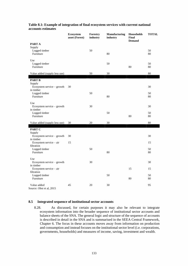
133

Table 8.1: Example of integration of final ecosystem services with current national

accounts estimates

Ecosystem

asset (Forest)

Forestry

industry

Manufacturing

industry

Households

Final

Demand

TOTAL

PART A

Supply

Logged timber 50 50

Furniture 80 80

Use

Logged timber 50 50

Furniture 80 80

Value added (supply less use) 50 30 80

PART B

Supply

Ecosystem service – growth

in timber

30 30

Logged timber 50 50

Furniture 80 80

Use

Ecosystem service – growth

in timber

30 30

Logged timber 50 50

Furniture 80 80

Value added (supply less use) 30 20 30 80

PART C

Supply

Ecosystem service – growth

in timber

30 30

Ecosystem service – air

filtration

15 15

Logged timber 50 50

Furniture 80 80

Use

Ecosystem service – growth

in timber

30 30

Ecosystem service – air

filtration

15 15

Logged timber 50 50

Furniture 80 80

Value added 45 20 30 95

Source: Obst et al, 2015

8.5 Integrated sequence of institutional sector accounts

8.28. As discussed, for certain purposes it may also be relevant to integrate

ecosystem information into the broader sequence of institutional sector accounts and

balance sheets of the SNA. The general logic and structure of the sequence of accounts

is described in detail in the SNA and is summarised in the SEEA Central Framework,

Chapter 6. The focus in these accounts moves away from information on production

and consumption and instead focuses on the institutional sector level (i.e. corporations,

governments, households) and measures of income, saving, investment and wealth.

134

8.29. One of the main functions of the sequence of accounts is to demonstrate the

linkages between incomes, investment and balance sheets and, in this context, a key

feature of the standard SNA sequence of accounts is the attribution of consumption of

fixed capital (depreciation) to economic activities and institutional sectors as a cost

against income.

8.30. The type of presentation that emerges from this integration is shown in Table

8.2, taken directly from SEEA EEA Annex A6. Table 8.2 presents simplified versions

of two models (A and B). In the example, presented for a farm, a single ecosystem asset

provides a mix of ecosystem services (total of 110) of which 80 are used by the farmer

and 30 are the final consumption of households. The allocation is based on the assumed composition of the ecosystem services. Thus, the value of 80 for ecosystem services may be considered inputs to agricultural production and the value of 30 may be considered regulating services, such as air filtration, used by households.

8.31. All SNA production of the farmer (200) is recorded as final consumption of

households. For simplicity, no other production, intermediate consumption or final

consumption is recorded. It is to be noted that in the generation of ecosystem services,

the table above does not show any “inputs” from the ecosystem (i.e. intermediate

ecosystem services). Recording these flows is not required for the purposes of

developing a sequence of accounts focused on economic units.

8.32. As shown in the previous example (table 8.1), in models A and B, the rise in

GDP occurs in relation only to the final consumption of ecosystem services that relate

to non-SNA benefits, i.e. the air filtration services of 30 units. This final consumption

is also attributed to households and leads to a final measure of GDP (gross value added)

in both models A and B of 230. In Model A, the GDP is allocated between the value

added of the farmer (120) and the value added of the ecosystem asset (110). In Model

B, all of the value added is attributed to the farmer on the assumption that it is the

economic unit that manages the ecosystem asset and hence the generation of ecosystem

services.

8.33. Having derived extended measures of GDP, these measures can now be

adjusted for the cost of capital in the derivation of that GDP. This includes the

deduction of depreciation (consumption of fixed capital) of produced assets, depletion

of natural resources and ecosystem degradation. In the SNA, only depreciation is

deducted to provide a measurement of net domestic product (NDP). Deduction of all

costs of capital provides a measure termed degradation adjusted NDP. In Table 8.2,

total deprecation is 10 units and ecosystem degradation is 15 units.

8.34. At an economy wide level, the resulting measure of degradation adjusted NDP

(205 units) will be the same irrespective of the choice of model A or B – assuming no

cross-border flows in relation to ecosystem services. However, when compiling

institutional sector accounts where the economy wide results are allocated between, for

example, corporations, governments and household sectors, a choice is required to

move forward concerning whether (i) ecosystems should be treated as producing units

in their own right - Model A; or (ii) treated as assets owned and managed by existing

economic units – Model B.

8.35. In the Technical Recommendations, no explicit recommendation between

Model A and B is provided. Discussion on other issues in ecosystem accounting

suggests treating ecosystem assets as distinct producing units fits neatly with logic of

measurement in other parts of the ecosystem accounting framework, particularly on

recording the supply of ecosystem services.

8.36. The significant implication of recognising ecosystem assets as a distinct sector

is that all ecosystem degradation is deducted from the value of the ecosystem services

generated by those assets. That is, the degradation is allocated to the ecosystem assets

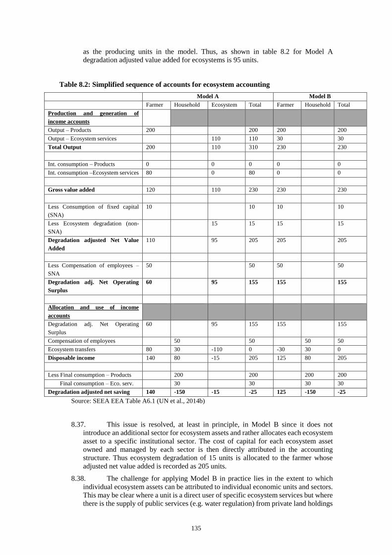
135

as the producing units in the model. Thus, as shown in table 8.2 for Model A

degradation adjusted value added for ecosystems is 95 units.

Table 8.2: Simplified sequence of accounts for ecosystem accounting

Model A Model B

Farmer Household Ecosystem Total Farmer Household Total

Production and generation of

income accounts

Output – Products 200 200 200 200

Output – Ecosystem services 110 110 30 30

Total Output 200 110 310 230 230

Int. consumption – Products 0 0 0 0 0

Int. consumption –Ecosystem services 80 0 80 0 0

Gross value added 120 110 230 230 230

Less Consumption of fixed capital

(SNA)

10 10 10 10

Less Ecosystem degradation (non-

SNA)

15 15 15 15

Degradation adjusted Net Value

Added

110 95 205 205 205

Less Compensation of employees –

SNA

50 50 50 50

Degradation adj. Net Operating

Surplus

60 95 155 155 155

Allocation and use of income

accounts

Degradation adj. Net Operating

Surplus

60 95 155 155 155

Compensation of employees 50 50 50 50

Ecosystem transfers 80 30 -110 0 -30 30 0

Disposable income 140 80 -15 205 125 80 205

Less Final consumption – Products 200 200 200 200

Final consumption – Eco. serv. 30 30 30 30

Degradation adjusted net saving 140 -150 -15 -25 125 -150 -25

Source: SEEA EEA Table A6.1 (UN et al., 2014b)

8.37. This issue is resolved, at least in principle, in Model B since it does not

introduce an additional sector for ecosystem assets and rather allocates each ecosystem

asset to a specific institutional sector. The cost of capital for each ecosystem asset

owned and managed by each sector is then directly attributed in the accounting

structure. Thus ecosystem degradation of 15 units is allocated to the farmer whose

adjusted net value added is recorded as 205 units.

8.38. The challenge for applying Model B in practice lies in the extent to which

individual ecosystem assets can be attributed to individual economic units and sectors.

This may be clear where a unit is a direct user of specific ecosystem services but where

there is the supply of public services (e.g. water regulation) from private land holdings

136

complete allocation of an asset (and its value) to a single institutional sector may not

be appropriate.

8.39. To explain this from an full accounting system approach, in this example, by

allocating all of the ecosystem asset to the farmer it could imply that the full value of

the ecosystem asset to the farmer should be recorded on the farmer’s balance sheet

including both the ecosystem services used as input to farm production and the publicly

consumed air filtration services. This may not provide a suitable recording for the

allocation of assets on the balance sheet.

8.40. The issue to be resolved is the balance between the allocation of the costs of

degradation to an appropriate economic unit and the attribution of the value of

ecosystem assets to the economic unit to the appropriate user of the services. The same

accounting challenge was confronted in the allocation of depletion of mineral and

energy resources in the SEEA Central Framework. The resolution in that case was to

show a series of transfers such that the depletion cost was attributed to the unit

extracting the resources and the balance sheets reflected the future income streams

attributable to two sectors (the mining and general government units). Similar transfers

could be envisaged for ecosystem accounting purposes but this recording has not been

developed at this stage.

8.41. It is noted that the approach to the allocation of degradation in some cases may

be relatively straightforward. However, in many other cases, the nature of the impacts

of economic activity on the environment are complex. For example, the impacts may

occur in areas well away from the source of the impact, may occur in time periods well

after the impact occurred, or may be unknown to the relevant units. In addition, it is

not necessarily clear in what way the loss of benefits incurred by the impacted sectors

should be related to the income of the sector causing the impact. These matters have

been debated at length in the national accounting community without any clear

resolution. Thus, while an appropriate accounting treatment can be determined, the

application of a treatment in practice and a recommendation on a preferred approach

will require further discussion of the appropriate treatments in a range of cases where

economic and human activity leads to degradation of ecosystem assets.

8.42. The final section of table 8.2 concerns the allocation and use of income

accounts. The aim of these accounts is to provide a measure of saving for the economy

as a whole and for each sector. For Model A, this requires recording an adjustment

titled “ecosystem transfers” that reflects that the farmer and the household sector need

resources to purchase ecosystem services from the ecosystem assets. Recording these

transfers allows the saving of the three sectors in Model A to reflect the actual cash

positions, recognising that flows of depreciation or degradation do not affect the cash

position.

8.43. In Model B, these ecosystem transfers are not required since there is no stand-

alone ecosystem sector. The difference in net saving for farmers between Model A and

Model B simply reflects that in Model B the ecosystem degradation of 15 units is

allocated to the farmer thus reducing the net saving to 125 units.

8.6 Extended and integrated balance sheets

8.44. The second type of integrated accounts are balance sheets, in which the

opening and closing values of ecosystem assets in monetary terms, as recorded in the

ecosystem monetary asset account, are integrated with the values of asset and liabilities

recorded in the standard balance sheet of the SNA. Such an integration would lead to

the derivation of extended measures of national and sector net wealth.

137

8.45. The integration of ecosystem asset values would seem a relatively

straightforward step. However, for a variety of reasons, it is likely to be quite complex.

There are two main challenges that are described at more length in SEEA EEA Chapter

6. First, in a full SNA and SEEA Central Framework balance sheet, there will already

be values recorded for natural resources, such as timber and fish. Since the value of

these resources is embedded in the value of ecosystem assets, via the valuation of

provisioning services, it will be necessary to appropriately ensure the value of natural

resources is not double counted. This issue will also apply to various cultivated

biological resources, such as orchards and vineyards.

8.46. Second, in many countries, the value of land will be recorded on the SNA

balance sheet estimated in terms of its market price. Since there is a generally well-

established market in land, balance sheet values may be obtained more directly than by

using net present value techniques as applied in resource accounting. It is likely to be

the case that the market values of land, particularly agricultural land, will capture the

value of some ecosystem services, at least to some extent. However, they are unlikely

to capture a full basket of ecosystem services, particularly those that have clear public

good characteristics and longer-term benefits. Also, the land value may well reflect

aspects that are not ecosystem services in nature – for example, the location and the

value of alternative uses (e.g. for urban development). Adjusting market values of land

for these considerations will require careful consideration.

8.47. In comparing the values of ecosystem assets with values currently incorporated

into SNA balance sheets, it is important to recognise the different underlying scopes of

environmental assets. In broad terms, the SNA balance sheets will have lower values

for environmental assets as a result of the SEEA EEA including the values of additional

ecosystem services. At the same time, the SEEA EEA values of ecosystem assets do

not cover all environmental assets – most notably sub-soil mineral and energy

resources34. The effects of these two differences on the total value of environmental

assets will vary from country to country.

8.48. A final challenge in the area of integrating the accounts arises when applying

the accounting approach at the level of an individual ecosystem asset. Recall that the

valuation of an ecosystem asset is directly related to the basket of final ecosystem

services that are expected to be generated from an asset. At the level of individual

ecosystem assets however, there will be cases where an asset supplies few, or no, final

ecosystem services (for example, a high mountain forest) but, instead plays a

supporting role in supplying intermediate services to neighbouring ecosystems. In this

situation, an ecosystem asset may be recorded as having zero monetary value and its

value becomes embodied in the value of the neighbouring ecosystems. While at an

aggregate, national level this may not be a significant issue, it is likely to be of concern

if attribution of value is being examined or accounting is being undertaken at smaller

sub-national scales. Resolution of this issue requires the incorporation of intermediate

services into the ecosystem accounting model in an explicit manner and associated

work to record dependencies between ecosystem assets.

8.49. From a national accounting perspective, the development of a sequence of

accounts and balance sheets represents an important objective that helps to motivate

the development of other parts of the ecosystem accounting framework. At the same

time, it is clear that: (i) work is needed to progress the development of the ecosystem

accounts which must underpin the integrated accounts described here; and (ii) that

further research and testing is needed to meet the challenges posed by integration.

Consequently, it is recommended that countries focus their efforts on developing

34 Accounting for these environmental assets is described in the SEEA Central Framework.

138

ecosystem extent and condition accounts and ecosystem services supply and use

accounts. There is tremendous value in these accounts in their own right.

8.7 Alternative approaches to integration

8.50. The sections above describe integration with the institutional sector accounts

and balance sheets following standard SNA measurement definitions and boundaries.

This is a natural objective for the SEEA and will be important when seeking to use data

already published in the national accounts, for example on national wealth and saving,

as the starting point for extension using ecosystem accounting data. However, there are

other integrated measurement approaches that do not apply SNA standard

measurement definitions and boundaries and hence provide alternative approaches to

the integration of ecosystem and economic data. Three alternative integrated

approaches are summarised here.

8.51. A well-developed approach, usually referred to as wealth accounting, has

developed as a branch of economics since the mid-1970s. Wealth accounting seeks to

aggregate the value of all relevant assets/capitals including produced, natural, human

and social capital. The most prominent work has been completed by the World Bank

(2011) and by UNU-IHDP and UNEP (2014). Their methods vary in the detail but they

are broadly similar approaches.

8.52. In concept, wealth accounting aims to value each form of capital in terms of

its marginal contribution to human welfare (Dasgupta, 2009; Arrow et al., 2012). By

doing so shadow prices are estimated for each asset type. From a national accounting

perspective while a focus on marginal prices is appropriate, estimation of the

contribution to welfare is different from a focus on exchange value.

8.53. Given the purpose of wealth accounting, the conceptual approach to integration

is quite appropriate. However, in practice, often values for produced assets from the

standard national accounts based on exchange values are combined with valuations for

other capitals based on welfare valuation concepts. Hence, there may be a lack of

alignment between the valuation approaches for different capitals. For natural capital,

it is clear that the use of exchange values for ecosystem services would not correspond

directly to the conceptual requirements of wealth accounting, although there will be

strong connections between the two approaches.

8.54. A second approach to integration builds on the use of restoration costs as a

measure of ecosystem degradation and records corresponding ecological liabilities on

the national balance sheet. That is, unpaid restoration costs that arise when an

ecosystem declines in condition are treated as a liability. This approach is described as

a possible extension in the ENCA QSP (Weber, 2014a) and has also been suggested

for use at the corporate level by the UK Natural Capital Committee. From a national

accounting perspective, there are a number of difficulties with this approach:

• First, there is the question of whether restoration costs are a suitable estimate

of ecosystem degradation, as discussed in chapter 7.

• Second, there is a question of when liabilities should be recognised. If there is

no expectation that the restoration will take place then, at least for accounting

purposes, no liability should be recognised. In effect, recognising these

liabilities is in the first instance a social or analytical choice rather than an

application of accounting principles.

• Third, if a liability is recognised then, all else being equal, net wealth should

fall by that amount. However, since the recognition of the liability reflects the

degradation of an asset there will be both a fall in an asset and an increase in a

139

liability for the same event. This implies a double counting on the balance sheet

in terms of the impact on net wealth. This issue does not arise in the integrated

accounting approach described earlier in this chapter since the only balance

sheet change is the fall in the asset value due to degradation. An alternative

solution to the double counting issue would be to record the liability but keep

the ecosystem asset value unchanged but this seems counter-intuitive.

8.55. Overall, while recording ecological debts seems attractive and may be a useful

tool in communicating the extent of ecosystem degradation, it has some deficiencies in

terms of its consistency with national accounting principles.

8.56. The final integrating approach described here is that of full cost accounting.

This is an accounting approach that has developed in corporate accounting. The intent

behind full cost accounting is to estimate and record the broader costs of a company’s

impacts on the environment as part of their ongoing operating costs thus resulting in

an adjusted profit and loss statement. For example, the costs of GHG emissions and the

release of pollutants are common areas of interest. Such information may be helpful in

a range of management situations.

8.57. From an ecosystem accounting perspective, a few points can be noted. First,

the approach largely excludes consideration of ecosystem services in terms of

recognising ecosystem services as inputs to the production process. Hence, within the

full cost accounting approach there is no change in the standard production or income

boundaries.

8.58. Second, there is no recognition of ecosystem assets as part of the capital base

of a company and hence no impact on the company’s balance sheet or recording of

ecosystem degradation as a capital cost. It would be implicitly included in the adjusted

profit and loss statement to the extent that this degradation was part of the derivation

of costs associated with the specific impacts assessed, but this would not be a specific

focus.

8.59. Third, the incorporation of costs associated with residual flows (emissions,

pollutants, etc.) is not something undertaken directly in ecosystem accounting. In broad

terms, a focus on residual flows reflects the valuation of a company’s negative

externalities and externalities are specifically excluded from the national accounts. It

may be that, in fact, the attribution of these costs can be part of a measure of ecosystem

degradation. Further work is required to understand the links between the valuation of

externalities and ecosystem accounting, recognising that the links may be different for

different types of externalities.

8.60. Overall, while full cost accounting does represent a form of integration it is

somewhat different in scope and intent relative to the concepts and intent of ecosystem

accounting.

8.8 Recommendations

8.61. From a national accounting perspective, the potential to record the full

integration of ecosystem accounting information into the standard national accounts

and the derivation of adjusted estimates of GDP and other measures of economic

activity represents an important aspect of the SEEA. While recognising the need for

additional discussion, particularly on the allocation of degradation, the adoption of

ecosystem accounting has demonstrated that a full integration is conceptually possible.

8.62. At the same time, there are numerous challenges in measurement that must be

worked through. These particularly concern the aggregation of stocks and flows across

ecosystem services and ecosystem assets. These are important challenges to be

140

confronted through testing and on-going research. This chapter has described some

specific issues concerning integration but the measurement issues raised in other

chapters are equally relevant in working towards a complete integrated accounting

dataset.

8.63. While work continues on developing these full links between ecosystem and

economic data, there are other options that can be pursued. Combined presentations, as

described in SEEA EEA Chapter 6 and in this chapter, are important tools for

presenting data that support a comparison and discussion of environmental and

economic issues. It is strongly recommended that countries work towards the

development of combined presentations of data. Work in this area is likely to be

considerably supported by a focus on presenting data at meaningful spatial level.

8.64. As work within a country proceeds on ecosystem accounting, it is important

that any related or similar work on the integration of environmental and economic data

is placed in context. Generally, it is not a question of data being in competition, but

rather it is a case of different data being suited for specific purposes. Explaining the

link between different measurement approaches and different policy questions is an

important role for national statisticians.

141

9 Thematic accounts

Key points in this chapter

Thematic accounts are standalone accounts on topics of interest in their own right and also of direct

relevance in the measurement of ecosystems and in assessing policy responses.

The thematic accounts described in this chapter cover accounts for land, carbon, water and species-level

biodiversity and reflect the discussion of these accounts in the SEEA Central Framework (for land and

water) and in the SEEA EEA (for carbon and species-level biodiversity).

Land accounts can focus on land use, land cover and land ownership. The development of land accounts

provides a platform for measurement and is commonly the basic entry point for ecosystem accounting.

In water accounting measurement at the water catchment level is important for ecosystem assessment.

Working at this level will require the use of hydrological models but this work can also underpin the

estimation of relevant ecosystem services such as water filtration and soil retention.

Accounting for stocks of carbon can provide a strong base for co-ordinating information on carbon and

complements measurement within the Inter-governmental Panel on Climate Change (IPCC) framework

and the UN REDD+. The data can support measurement of ecosystem condition and ecosystem services

such as carbon sequestration.

Accounting for biodiversity considers both ecosystem and species-level biodiversity. Biodiversity is

considered primarily a characteristic of ecosystem assets rather than an ecosystem service. In accounting

terms, this permits recognition of declines or improvements in biodiversity over time and links to the

capacity of ecosystems to supply ecosystem services.

In all cases - land, water, carbon and biodiversity - there is a broad range of information and measurement

methodologies available. The challenge for ecosystem accounting is the assessment and integration of

these data and methods within the SEEA EEA framework.

9.1 Introduction

9.1. The ecosystem accounts described in earlier chapters provide a coherent

coverage of information pertaining to ecosystem assets and ecosystem services. At the

same time, from both an analytical and a measurement perspective, it can be

challenging to focus only on a systems perspective. More commonly, our view of

ecosystems, and our policy responses, are framed using themes that concern specific

aspects of the economy–environment relationship. Four themes that are consistently

evident are land, water, carbon and biodiversity. This chapter summarises accounting

in relation to these themes reflecting the more detailed discussion of accounting for

these themes in the SEEA Central Framework and the SEEA EEA.

9.2. The incorporation of a thematic focus in the context of ecosystem accounting

provides two benefits. First, it enables a closer link to be drawn between the

compilation of ecosystem accounts and the likely areas of policy response – for

example in terms of land management, management of catchments, carbon emissions

policy and maintenance of protected areas.

9.3. Second, the data that are used to understand trends in thematic areas can also

be used to compile ecosystem accounts. This can be seen from two perspectives, first

from the practical perspective that entries in the ecosystem accounts can be sourced

from thematic accounts (e.g. estimates of water provisioning services from water

accounts); and second, recognising that a number of the thematic accounts can be

considered to each measure distinct ecological functions or cycles – i.e. the carbon

cycle the hydrological cycle, etc. In this sense, the thematic accounts provide a different

but comprehensive information to support ecosystem accounting.

9.4. It is relevant to note that while measurement in each of the four main themes

is relatively well advanced, the work on the SEEA has highlighted the potential to use

142

accounting approaches to (i) improve the co-ordination of data and (ii) recognise links

between the themes.

9.5. In the case of two themes – land and water – the SEEA Central Framework

and the SEEA Water provide the conceptual grounding for accounting. For carbon, as

a single element, it is actually quite well suited as a subject for accounting. It has thus

been relatively straightforward to consider adapting the measurement of carbon into a

broad accounting structure. The relevant concepts are described in the SEEA EEA. For

biodiversity, the application of accounting principles continues to develop. SEEA EEA

section 4.5 introduced relevant ideas for accounting for biodiversity but further work

has taken place reflected in a report completed by UNEP-WCMC (2016) and further

testing continues.

9.6. Accounts for land, water, carbon and biodiversity contain much relevant

information in their own right. Consequently, compilers of ecosystem accounts are

encouraged to seek opportunities to promote and use the information presented in these

thematic accounts to support discussion of environmental-economic issues. In

particular, information from the thematic accounts, when presented in the context of

ecosystem condition and services measures, can provide a more tangible hook for users

when making links between ecosystems and policy choices.

9.7. This chapter provides a summary of the relevant accounting issues for each of

these four areas and, in section 9.6, other potential thematic accounts are described.

9.2 Accounting for land

9.2.1 Introduction

9.8. Following the accounting principles and structures described in the SEEA

Central Framework, accounting for land, particularly land cover, will be a common

starting point for compilers of ecosystem accounts. A distinction is made here between

land accounting and ecosystem extent accounts. Land accounting is considered to

encompass compilation of a variety of accounts utilising different classifications of

land including land use/management, land cover, and land ownership. In applying these

classifications, links to standard SNA classifications of industry (ISIC) and institutional

sector. Land accounting incorporates standard asset account structures and also change

matrices and tables that cross-classify areas of land, for example land cover cross

classified with land ownership (by institutional sector). These various aspects of land

accounting are covered in the SEEA Central Framework Chapter 5.

9.9. Ecosystem extent accounts, described in Technical Recommendations chapter

3, are a specific account recording the area and change in area of different ecosystem

types (ET). The classification used for ecosystem extent accounting should reflect

aspects of both land use and land cover and hence generally an extent account will be

similar in structure to land accounts from the SEEA Central Framework but will differ

in the types of areas being accounted for. At an aggregate or initial level, it may be

necessary to define classes of ET on the basis of land cover classes. In this case the

ecosystem extent accounts and land cover accounts (as described in the SEEA Central

Framework) will be equivalent.

9.10. While the detailed ET classes may be different, as part of the accounts

compilation process, the information from land cover accounts can be used to help

define the relevant spatial areas, to determine the extent of different ecosystem types

at a broad level, to support understanding the links between ecosystem services supply

and the beneficiaries of those ecosystem services and finally, to facilitate the scaling of

other data to finer and broader levels of detail.

143

9.11. Further, from an analytical and policy perspective, information on land cover

can, at a national scale, provide important information on trends in deforestation,

desertification, urbanisation and similar forms of landscape change. As recognised in

ecosystem accounting, understanding these types of changes is not sufficient for

understanding the effects on ecosystem condition or flows of ecosystem services but it

is a relevant starting point.

9.12. As noted above, the total area of a country may also be classified according to

land use or land ownership criteria. An interim land use classification is provided in

the SEEA Central Framework (Table 5.11 and Annex I). Land ownership may be

classified by institutional sector (corporations, government, households) or by industry

(agriculture, manufacturing, retail, etc.). In some cases, a reasonably clear connection

can be made between different classifications of land – for example there will often be

a connection between tree-covered areas and forestry. However, it is not possible for a

simple integration of land cover and land use classes to be described.

9.13. Information on land use and land ownership will be important in understanding

the connection between ecosystem assets and the users of ecosystem services. For that

reason, it is recommended that, where possible, accounts for land use and land

ownership be compiled following the advice in the SEEA Central Framework. A useful

output for ecosystem accounting may be a table which cross-classifies land cover and

land use at a given point in time. Such a table would highlight the relative significance

of different land cover types to specific uses.

9.14. Land accounts can also provide an important tool to link environmental and

socio-economic data, essentially providing a means by which policy can be placed in

a spatial context. A key link here is recognising that implementation of policy to

maintain and restore ecosystem condition is likely to require the involvement of land

holders. Hence, understanding the connection between land ownership, current use and

the relevant ecosystem types can provide the means by which decisions on appropriate

policy interventions can be made.

9.15. Generally, the initial focus of land accounting is on terrestrial areas of a

country, including freshwater bodies. Within this scope land must be classified into

various classes (type of cover, type of use, or type of owning economic unit). Often

there will be relevant national classifications and datasets but alignment or

correspondence to international classifications is a positive step. Chapter 3 discusses

issues of classification in more detail.

9.16. As recognised in chapter 3, and in the SEEA Central Framework, accounting

for ecosystem extent and land can be extended to encompass marine and coastal areas.

Work on marine and coastal ecosystems in an ecosystem accounting context is

developing as referenced in chapter 3 and no further articulation is provided in this

chapter.

9.17. The basic structure of a land account follows the structure of an asset account

as described in the SEEA Central Framework. That is, there will be an opening stock,

additions and reductions in stock and a closing stock. Ideally, changes in stock over an

accounting period are separated into those that are naturally driven and those due to

human activities.

9.18. In addition to an asset account, information on land cover and land use may be

organised in the form of properly vetted and quality controlled change matrices which

show how, over an accounting period, the composition of land has changed. An

example of such a matrix for land cover is provided in the SEEA Central Framework,

Table 5.14 (UN et al., 2014a).

144

9.2.2 Relevant data and source materials

9.19. Ivanov (2015) discusses the compilation of land accounts in more detail. In

terms of data requirements, that paper distinguishes between dynamic and permanent

features. Dynamic features include information on land use, land cover and vegetation

type. Permanent features include information on administrative boundaries, ecological

regions, and river basins. Combinations of both administrative boundaries and

ecological regions, such as Statistics Canada’s (2016) Census Metropolitan Area-

Ecosystems (CMA-E), can also be developed when appropriate.

9.20. The compilation of accounts will generally require bringing these various data

together using GIS systems to produce data for a country as a whole. The ambition in

accounting terms is to generate harmonised maps, in time series, such that the stock

and changes in stock can be consistently accounted for.

9.21. Materials to support land accounting include the SEEA Central Framework,

the SEEA EEA and the ENCA QSP. The ENCA QSP in particular has an extensive

discussion of land cover accounting and associated data sources and methods.

9.22. Additional support and guidance is available in looking at country examples

and case studies. Relevant examples include the work of the European Environment

Agency (Weber, 2011), the ABS (2015), Statistics Canada (2013), the Victorian

Department of Sustainability and Environment (2013) and in Mauritius (Weber,

2014b).

9.2.3 Key issues and challenges in measurement

9.23. There is a range of measurement challenges in land accounting. An immediate

challenge is being able to integrate the various data to produce harmonised geo-

databases and, for accounting purposes, measures of change over time. This requires

careful consideration of scale and classification in combining different data sets at the

same point in time and the same data set at different points in time.

9.24. In general terms, higher levels of detail will be better but will also have higher

resource costs. Balancing the resources available with the degree of accuracy required

will be important. A relevant issue in this context is understanding approaches to the

validation of data, particularly since much data will be derived from remote sensing

(earth observation) sources, including satellite imagery. Ideally, some degree of

sampled ground truthing must be undertaken or some other quality control and data

confrontation process, for example comparison to administrative data, information

from agricultural and population census or other sources35.

9.25. The Land Use and Cover Area Survey (LUCAS) has been developed in recent

years by Eurostat following an integrated approach involving sampled reference points

to measure land use and land cover across Europe. This approach may provide

additional ideas for measurement approaches at national level.

9.26. The approach to classifying land is particularly important for communicating

messages on the changing composition of land at national level. For land cover, there

is now an ISO standard36 that underpins the Land Cover Classification System (LCCS

version 3) as developed by the FAO (FAO and GLCN, 2009). This provides a structure

by which each type of land cover around the world can be consistently classified. It

35 For example, the FAO has used sampled locations from Google Earth to “ground truth” its satellite based

estimates of land cover. 36 ISO 19144-2:2012 specifies a Land Cover Meta Language (LCML) expressed as a UML metamodel that

allows different land cover classification systems to be described based on the physiognomic aspects.

http://www.iso.org/iso/iso_catalogue/catalogue_tc/catalogue_detail.htm?csnumber=44342

145

thus provides a way of linking the various land cover classifications that are in use in

different countries and regions.

9.27. While this provides a base level classification tool, the approaches to the

formation of higher level classes that can be used to summarise detailed classes in

meaningful ways have been more varied. There are a number of options, one of which

is the interim land cover classification presented in the SEEA Central Framework.

Establishing a broadly accepted set of high level (say 10-15) classes of land cover (and

the associated definitions of these classes) would be a significant step forward in

coordinating information. It would further underpin greater alignment in ecosystem

accounting discussions and applications. At the same time, for analysis of changes over

time, a smaller number of classes may be most appropriate to ensure that the

measurement of change is as accurate as possible.

9.28. With regard to the classification of land use, the SEEA Central Framework

describes an interim land use classification with seven high level classes of land use

based on work on agriculture, forestry and fisheries land use by the FAO, and UN

Economic Commission for Europe (UNECE) work on the classification of land use for

all economic activities. It also introduced classes concerning inland water, coastal

waters and marine areas extending to a country’s exclusive economic zone (EEZ). The

finalisation of classifications for land use and land cover are a priority on the research

agenda for the SEEA Central Framework.

9.29. It should be recognised that the use of land cover and land use data reflects the

use of two dimensions to represent a three-dimensional world. In the context of

multiple class datasets, this can lead to significant trade-offs in measurement of

individual classes and potential biases. In particular, differences will likely emerge in

comparing the results for a given ecosystem type (e.g. wetlands) from a multiple class

land cover datasets and from a single class dataset that is specifically designed to

consider that ecosystem type. Where possible, it is recommended that information from

single class datasets is used and integrated within the broader coverage required for the

accounts.

9.2.4 Recommended activities and research issues

9.30. It is recommended that countries develop land accounts as an integral part of a

suite of national environmental-economic accounts. In their own right, land accounts

provide important information on environmental trends. Also, their compilation

requires the organisation of spatial data which in turn provides the inputs for the

delineation of spatial units and ecosystem accounting. Finally, a focus on land provides

a platform for integrating environmental and socio-economic data.

9.31. A number of relevant areas for testing land accounts are presented in chapter

3 in relation to the delineation of spatial units and the compilation of ecosystem extent

accounts. In terms of areas for research, the main issues, beyond those already noted in

chapter 3, concern (i) finalising appropriate classifications for land cover and land use

beyond the interim classifications of the SEEA Central Framework; and (ii)

determining the best approaches to account for linear features, such as rivers, beaches

and hedgerows.

9.32. From a practical perspective, testing and additional advice needs to be

provided on:

• The interpretation of land cover and use data, particularly in the context of

using remote sensing and satellite data.

• Understanding the appropriate scale for land accounts and the

measurement of spatial areas

146

• Techniques for controlling land cover and land use data sets for quality,

especially techniques for ground truthing data.

• Methods for developing time series of data on land cover and land use

change, including the use of information on disturbances such as forest

fires.

• Approaches to identifying key and rare ecosystem types which may be

relatively small in a national context.

9.3 Accounting for water related stocks and flows

9.3.1 Introduction

9.33. Water is a fundamental resource. It is essential for all life and underpins the

production of food, fibre and energy in many countries. The management of water,

including taking into account cross-boundary flows (e.g. the Nile River), and the joint

ownership of surface water bodies (e.g. Lake Victoria), is an important focus for many

governments around the world.

9.34. Accounting for stocks and flows of water is a key feature of the SEEA Central

Framework, the SEEA Water and the SEEA EEA. Whatever the context, accounting

for water resources should be undertaken following the standard advice in the SEEA

Central Framework. This short section is intended only to provide direction to relevant

technical and compilation materials rather than reproduce or summarise the content of

the SEEA manuals.

9.35. Accounting for water is relevant to ecosystem accounting in a number of ways.

First, water is a key feature of ecosystems and hence the measurement of the stocks

and changes in stocks of water resources is a relevant aspect in the measurement of

ecosystem condition. Accounting for changes in water quality would also be an

important contribution to ecosystem accounting but this area of water accounting is not

well developed from a SEEA perspective.

9.36. Second, there are a number of ecosystem services which relate directly to

water. These include the provisioning service of water when it is abstracted for use

(irrigation, drinking, hydropower), the regulating role of water bodies in filtering

pollutants and other residual flows, and the cultural services associated with water such

as fishing and other recreational activities. In addition, there are a number of ecosystem

services to which water is linked, for example, the regulation of water flows to provide

flood protection benefits and the filtration of water by ecosystem assets.

9.37. Measurements in all of these areas are ultimately important within a complete

set of ecosystem accounts. The water resource accounts of the SEEA Central

Framework and the SEEA Water focus on two areas – (a) the supply and use of water;

and (b) the asset account for water. They provide the basis for accounting for stocks

and flows of water. Of particular note is that the accounting can be undertaken at a sub-

national level and compilation at catchment level is recommended.

9.38. At the level of individual water catchments or basins, information may be

available that provides a characterisation of each catchment, for example using

information on temperature, precipitation, population density, nutrient flow, barrier

density, fragmentation, etc. Such information will support the compilation and

interpretation of ecosystem accounts.

147

9.3.2 Relevant data and source materials

9.39. There are many relevant materials to support the compilation of water

accounts. Aside from the content in the SEEA Central Framework and the SEEA EEA,

there is also SEEA Water (UN, 2012b) and the associated International

Recommendations on Water Statistics (IRWS) (UN, 2012a). Chapter 6 of the ENCA

QSP also describes much relevant information.

9.40. There is a wide range of data sources, including global data sets that might be

considered for use in water accounting. Vardon (2014a) provides a good overview and

links to these data sources, and also provides a description of some relevant country

examples. In some cases, the use of GIS tools will be relevant to estimate water stocks

and flows in areas that are not regularly gauged or where observed data are not

available. To date, over 50 countries have trialled the development of SEEA based

water accounts. Consequently, there is a broad and increasing body of knowledge and

experience in water accounting that can be drawn on.

9.3.3 Key issues and challenges in measurement

9.41. There remain some specific challenges in accounting for water, especially in

an ecosystem accounting context. Linked to the issue of defining spatial units, there is

the need for clarity on the delineation of wetlands with the scale of analysis being a

particular area of concern. Many wetlands may be quite small but disproportionately

important within larger land cover types (for example, in grasslands).

9.42. To more fully incorporate information pertaining to the hydrological cycle,

integrating information on groundwater within the ecosystem accounting framework

requires further consideration. To date ecosystem accounting has generally focused on

surface water resources. The incorporation of the atmosphere would also be relevant in

this context.

9.43. Integration of information on stream flow and water yield will also be

appropriate. While these are not standard SEEA accounting entries, indicators on these

aspects of the hydrological system will be relevant in understanding the system and

more completely assessing ecosystem condition. Indeed, in some countries with very

large stocks of water resources, understanding the stock of renewable water (based on

information on stream flow and water yield) may be of direct use in understanding the

relationship between water resources and socio-economic activity.

9.44. Given that flows of water are often key pathways between different

ecosystems, more work is needed to understand and account for flows of intermediate

ecosystem services and dependencies between ecosystem assets that are related to

water. For example, understanding water flows is relevant in measuring the service of

soil retention within a water catchment. SEEA EEA largely ignored flows between

ecosystems but further reflection suggests that incorporating certain intermediate

ecosystem services is required.

9.45. A general challenge in water accounting from a national accounts perspective

is that national data on stocks and flows of water resources may not be overly

meaningful. Instead, standardized information at a catchment level is required. While

it may be straightforward to propose measurement at this level of detail, developing

estimates at a catchment level will be resource intensive. Further, in some situations,

sub-annual (including daily) data may be needed to understand the dynamics of

seasonal fluctuations in water supply and water use (see, for example, Statistics

Canada, 2010). Such an understanding will be missed if working only with annual data

or long-term averages.

148

9.3.4 Recommended activities and research issues

9.46. The main conclusion in relation to accounting for water resources is that there

is a wide array of information and examples of water accounting in practice to support

countries that wish to start work in this area. Further, there are many datasets that can

provide a starting point for compilation. Testing the compilation of water accounts can

therefore be given a very high priority.

9.47. Vardon (2014a) highlighted a number of areas in which further research might

be conducted. These include accounting for dependencies between ecosystem assets

within catchments (including flows of intermediate ecosystem services), advancing

discussion on the valuation of water resources and accounting for water quality at a

broad scale. Further, the integration of information on groundwater and atmospheric

water would complement the information in both water resource accounts and

ecosystem accounts.

9.4 Accounting for carbon related stocks and flows

9.4.1 Introduction

9.48. Carbon has a central place in ecosystem and other environmental processes

and hence accounting for carbon stocks and transfers between them must be seen as an

important aspect of environmental-economic accounting. This short section is intended

only to provide direction to relevant technical and compilation materials rather than to

reproduce or summarise the content of those materials.

9.49. Accounting for carbon in the SEEA commenced in the context of accounting

for carbon stored in forests and for GHG emissions. Accounting for these stocks and

flows of carbon was included in the SEEA Central Framework. With the development

of the SEEA EEA, the scope of carbon accounting has been broadened. Ideally, it

encompasses measurement of carbon stocks and flows for all parts of the carbon cycle

and all carbon pools. Thus, it covers geocarbon, biocarbon, atmospheric carbon, carbon

in the oceans and carbon accumulated in the economy. In practice, the focus of carbon

accounting at this stage is on biocarbon and geocarbon.

9.50. The measurement of stocks and flows of carbon can support discussion of

many policy relevant issues. These issues include the analysis of greenhouse gas

emissions, sources of energy, deforestation and land use change, loss of productivity

and biomass, and sources and sinks of carbon emissions. Since carbon is also a common

focus of policy response, for example carbon taxes, its direct measurement is of high

relevance.

9.51. In ecosystem accounting, information on stocks and flows of carbon may be

used in two main areas. First, it may be considered as a broad indicator in the

measurement of ecosystem condition. For example, following Chapin et al. (2006)

changes in the net ecosystem carbon balance can be used as an indicator of ecosystem

condition. However, it should be recognised that in many contexts, the stock of biomass

carbon is generated through human actions (e.g. plantation forests) and consequently

measures of the carbon balance will provide poor measures of ecosystem condition if

used as a proxy for the degree of naturalness of the ecosystem. The second area of use

of carbon accounts in ecosystem accounts relates to the measurement of ecosystem

services including carbon sequestration.

149

9.4.2 Relevant data and source materials

9.52. The structure of a carbon stock account is presented in SEEA EEA Chapter 4.

The compilation of that account, with a focus on biocarbon and geocarbon, involves

the collection of (i) data on land vegetation/cover and the rates at which different

land/vegetation cover types sequester and store carbon in above and below ground

biomass; (ii) data on the carbon content of soils; and (iii) information on sub-soil fossil

fuel resources. A summary of relevant data sources and links to those sources is

presented in Vardon (2014b). A particularly relevant source is information compiled

by countries as part of reporting to the IPCC although not all land types are included

under the Kyoto Protocol.

9.53. Advice on the compilation of carbon accounts is summarised in the SEEA

EEA. A more detailed explanation is provided by Ajani and Comisari (2014) which

describes the development of a carbon account for Australia including discussion of

the relevance and application of the account.

9.54. A number of aspects of carbon accounting are also reflected in the SEEA

Central Framework. For example, air emission accounts will include flows of GHG

emissions; and mineral and energy resource asset accounts will record stocks and

changes in stocks of sub-soil fossil fuel resources. Within the SEEA framing, all of the

information on these various parts of the carbon cycle should be able to be brought

together to provide a coherent picture of carbon stocks and flows for a country. For

SEEA EEA purposes, the key distinction is the need to compile carbon accounts at a

finer level of spatial detail, e.g. by EA or ET.

9.55. The ENCA QSP provides a detailed discussion on accounting for changes in

biocarbon at national scale including a discussion of global datasets and measurement

challenges. Of particular relevance, is the work undertaken on the measurement of

carbon through the FAO Forest Resource Assessment (FRA) (FAO, 2015) which is

conducted every five years. The FRA asks for estimates of carbon stock for forests

including above and below ground carbon stocks. These data may provide a useful

starting point for compiling a time series of carbon accounts. Further, they may provide

a sufficient level of detail by type of forest such that the interpretation of changes in

the carbon balance can be better associated to changes in ecosystem condition.

9.4.3 Key issues and challenges in measurement

9.56. Compared to other areas of measurement, the measurement issues in relation

to carbon have relatively well-researched, reflecting the substantial resources that have

been applied to this measurement task within the IPCC processes. Nonetheless, there

remain important issues of data quality to consider and challenges exist in using point

measurements for estimation of stocks of carbon across large scale areas and in

accounting for the wide variety of vegetation and soil types since different carbon

content ratios will apply in different situations. Related to these issues, the sourcing of

information via either remote sensing or using local sources requires balancing between

coverage and accuracy.

9.4.4 Recommended activities and research issues

9.57. Given the high policy relevance of carbon and the comparably large resources

directed at measuring stocks and flows of carbon at national level, it is recommended

that countries support the development of carbon accounts. The preparation of these

accounts can provide information on broad trends in environmental change and also

150

provide insight into the requirements of bringing data together from a variety of

sources.

9.5 Accounting for biodiversity

9.5.1 Introduction

9.58. Biodiversity - the diversity of ecosystems, species and genes - plays an

essential role in supporting human well-being. Biodiversity helps maintain functioning

and resilient ecosystems that in turn deliver ecosystem services such as food, the

regulation of our climate, aesthetic enjoyment and other cultural benefits.

9.59. The SEEA EEA provides a framework to measure and link ecosystem service

flows supported by biodiversity and other characteristics (e.g. soil type, altitude) with

the economy and other human activities. It also allows comparison and integration of

data on ecosystem services with other economic and social data. Biodiversity accounts,

in conjunction with the ecosystem accounting framework, can therefore help to build

an understanding of the relationship between biodiversity and economic activity.

9.60. On the whole, the perspective taken in the SEEA EEA is that biodiversity is a

characteristic that is directly relevant in measurement of the condition of ecosystem

assets. Measures of biodiversity are considered to relate primarily to ecosystem assets

in the accounting model. Thus, potential connections to biodiversity, such as

birdwatching or fishing, are considered derivative from biodiversity rather than flows

of biodiversity services in their own right. This approach is consistent with a view that

biodiversity can be degraded or enhanced over time, an attribute that applies only to

assets in an accounting context.

9.61. Further, people may appreciate, and therefore value, specific elements of

biodiversity, for example when they take an interest in the conservation of endemic

and/or iconic species. This is reflected, for instance, in the creation of protected areas

in many countries. These species can only survive in the long-term when the overall

condition of the ecosystems in which they occur is maintained, a logic that highlights

again the distinction between the measurement of specific ecosystem services, the

existence of individual species and ecosystem condition. The discussion of biodiversity

in accounting for ecosystem stocks and flows must therefore be undertaken with

appropriate care.

9.62. In the framing of the SEEA EEA, species-level biodiversity may be considered

as a characteristic of an individual EA or connected EAs (for example, EAs linked via

patterns of migration for certain species). Ecosystem-level biodiversity emerges from

assessment of the diversity of ET (depending on the suitability of the classification of

ecosystem types).

9.63. Notwithstanding the connection made here between biodiversity measurement

and the measurement of ecosystem assets, there are situations in which measures of

biodiversity can be indicators of flows of final ecosystem services. For example,

biodiversity indicators may be related to the value of recreational services from wildlife

related activities, where people gain benefit from experiencing the diversity of nature

(as distinct from services received from appreciation of individual species). In these

circumstances, it is relevant to recognise that measures related to biodiversity may be

appropriate indicators in a variety of accounts, including ecosystem condition accounts

and ecosystem services supply and use accounts.

9.64. Beyond supporting ecosystem accounting, biodiversity accounting also

provides opportunities for the harmonization of national level biodiversity data

alongside other reporting mechanisms, such as the CBD through the implementation

151

of National Biodiversity Strategies and Action Plans (NBSAPs) and reporting on the

SDGs.

9.65. In order to reflect the multi-layered relation between biodiversity, ecosystem

functioning, ecosystem services and the human appreciation of ecosystems, a range of

biodiversity indicators should be considered. Species indicators may be selected on the

basis of the importance of species for specific ecosystem processes, for being indicative

of ecosystem condition or functioning, or because the species represent specific aspects

that people appreciate in biodiversity, such as the occurrence or abundance of

threatened, endemic and/or iconic species.

9.66. Integrated accounting for aspects of biodiversity is still developing and

experimentation on biodiversity accounting by countries is less advanced than for water

or carbon accounting. To advance work, a paper was commissioned as part of the

ANCA project (UNEP-WCMC, 2015). This led to a follow up workshop and

publication, specifically focusing on exploring approaches to accounting for species in

the context of the SEEA EEA (UNEP-WCMC, 2016). This section summarizes the

findings of these outputs but does not attempt to provide definitive descriptions of

biodiversity or its measurement.

9.5.2 Assessing ecosystem-level and species-level biodiversity

9.67. Assessments of biodiversity generally consider ecosystem-level and species-

level biodiversity due to the cost and complexity of assessing genetic-level

biodiversity. However, genetic-level biodiversity is an important topic and may be

integrated into ecosystem accounting in the future.

9.68. Ideally, data should meet the following general criteria to be suitable for

accounting for biodiversity. The data should:

• Be accessible at a spatial resolution suitable for accounting. This allows data to be

mapped to individual ecosystem assets and types.

• Be temporally relevant. This informs net changes in the stock of biodiversity

between the opening and closing of accounting periods.

• Be comparable to a common reference condition. This allows the comparison of

biodiversity measures against a benchmark indicative of a balanced state and aids

aggregation of different types of biodiversity data.

• Be possible to aggregate the measures to provide a composite indicator of the

condition of biodiversity (e.g., via the Simpson Index or aggregation using a

common reference condition). The change in this composite indicator between

accounting periods provides an indication of the net biodiversity balance.

• Be comparable over space and time. This allows direct comparison of biodiversity

stocks in different ecosystem types.

9.69. Ecosystem-level biodiversity may be assessed using information on ecosystem

extent as described in Chapter 3. Extent measures are based on data on land cover, land

use, habitat and other ecosystem data, commonly sourced from satellite remote sensing.

Within the SEEA EEA framework, these data inputs also provide spatial information

for delineating ecosystem assets on the basis of common characteristics. Many

countries have their own ecosystem classification standards and methods for mapping

them, and work is progressing towards an internationally accepted ecosystem

classification.

9.70. When accounting for ecosystem-level biodiversity, it may be useful to

supplement information within the ecosystem extent account with more detailed

152

information on species, such as vegetation classes, community composition or other

characteristics. To best support integration, this work should be undertaken in the

context of the spatial areas defined for ecosystem extent accounting rather than for land

cover accounts as described in the SEEA Central Framework.

9.71. Given that ecosystem-level biodiversity is captured in the ecosystem extent

account, the focus of thematic biodiversity accounting in this chapter is on species-

level biodiversity. Ideally, the development of a biodiversity account using species data

should move beyond simple counts of the number of species (the species richness) and

include the population size of each species (the species abundance) as this provides

more information on the status of species.

9.72. The International Union for the Conservation of Nature (IUCN) Red List of

Ecosystems (Keith, et al., 2013) will, in due course, meet the criteria listed above by

generating measures of ecosystem condition based on risk of ecosystem collapse. The

spatial resolution will be high enough for national level ecosystem accounting

(anticipated to be at least 250m resolution). The first global assessment (scheduled for

2025) will provide a baseline which may then be used as a reference condition.

Assessments are likely to be repeated on a 5-year basis. The application of the

quantitative categories and criteria will ensure consistency and comparability between

countries and over time.

9.73. In regard to species-level biodiversity data, three approaches that are relevant

to different thematic biodiversity accounting concerns are noted here. First, the IUCN

Red List of Threatened Species (IUCN, 2014) which measures extinction risk.

Application of the IUCN Red List categories and criteria ensures consistency in

assessment over space, over time, and between assessors. While originally designed

for global assessments, methods are available to allow disaggregation of the Red List

Index to national levels. Downscaling of the global Red List to national levels can be

complemented with national red lists, where these exist. It is suggested that both the

global Red List and national red lists are used to ensure as broad and relevant a

coverage as possible.

9.74. Second, the Norwegian Nature Index (NNI) (Certain and Skarpaas, 2011) uses

indicators from a variety of species groups and major ecosystem types that measure

deviation from a reference state. The NNI produces a single ‘value’ that provides

information on the condition of species-level biodiversity (and other characteristics) in

ecosystems. The NNI incorporates expert judgment, monitoring-based estimates, and

model-based estimates, so the method can be used in both data rich and data poor areas.

9.75. Third, the Living Planet Index (LPI) (WWF, 2014) aggregates species

population trend data from different sources and across multiple spatial scales. The

methodology involves a series of aggregations in order to avoid bias induced by

including only well-known taxonomic groups and well-studied locations. With

systematic monitoring of species abundance, the data lends itself to incorporation in an

accounting format.

9.76. Species-level biodiversity is challenging to document and describe fully

because of the large number of different species and species occurrences, even in

relatively species-poor environments. Consequently, ecosystem-level biodiversity or

accounting for ecosystem types can provide a useful “coarse-filter surrogate” for

species-level biodiversity. If ecosystem-level biodiversity is reasonably well

documented through mapping and classifying different ecosystem types, much species-

level biodiversity is accounted for when ecosystem-level biodiversity is accounted for.

For example, a decline in ecosystem-level biodiversity would likely be accompanied

by a decline in species-level biodiversity.

9.77. There are a number of designations for ecologically important places that can

153

support species-level biodiversity measurement. These include Key Biodiversity Areas

(KBAs), Alliance for Zero Extinction (AZE) sites, Biodiversity hot-spots identified by

Conservation International, national parks and nature reserves. Accounting for the

extent of these areas also provide useful information on potential trends in species

status.

9.5.3 Implementing biodiversity accounting

9.78. A key starting point for biodiversity accounting is to identify biodiversity-

related policy priorities to help determine what information should be compiled,

covering plants, animals and to a lesser extent fungi. This step will also establish the

required resolution of data (both spatial and temporal) necessary to address these

priorities.

9.79. Establishing an inventory of all existing monitoring data will help identify any

‘data-gaps’. Identifying data gaps could inform a protocol for further data gathering

(e.g., via monitoring or modelling approaches). Countries should also consider their

reporting obligations to regional processes and biodiversity-related

conventions/agreements, such as the CBD or the Ramsar Convention.

9.80. Developing measures of species-level biodiversity is resource intensive and

has methodological challenges. A complete inventory of a country’s species is not

possible and so the species to be included in an account will need to be prioritized.

Some species (e.g. keystone or umbrella species) are better indicators of biodiversity

and ecological condition than others. Other species may be of particular relevance for

because of their functional roles (e.g., pollinating species), cultural importance (e.g.,

sacred plants and animals) or conservation concern (e.g., threatened species). When

selecting species, the broader the representation of taxonomic groups (e.g. plants, birds,

mammals etc.), the better the account will estimate overall biodiversity (see Remme et

al., 2016 for details). Instead of focusing purely on individual species, it may also be

useful to construct accounts for species groups (e.g., taxonomic, trophic or functional

groups).

9.81. Any prioritization exercise should be driven by the intended uses of the

biodiversity accounts. More than one species-level biodiversity account may be

required in order to answer the range of biodiversity relevant policy questions. For

instance, UNEP-WCMC (2016) proposes that prioritized species or species groups be

organized in either holistic accounts or in separate accounts of:

a. Species of conservation concern

b. Species important for ecosystem condition and/or functioning

c. Species important for ecosystem service delivery

UNEP-WCMC (2016) identifies that these accounts could be supplemented (or

substituted where data is limited) with accounts of Red List Status and / or accounts of

the extent of important places (Key Biodiversity Areas, National Parks, etc.).

9.82. When measuring species-level biodiversity, it is important to distinguish

between quantity and variation. Considering species-level biodiversity in terms of

quantity (e.g., abundance) will be important when accounting for the stock of particular

aspects of biodiversity is of interest. However, this does not reflect the emphasis of

variability implicit in the CBD’s definition of biological diversity (CBD, 1992). When

applied to species, this variation is expressed by alpha (within communities), beta

(between communities) and gamma (within a landscape) diversity. Therefore, when

creating a Species Account, analysts should consult with ecologists to ensure

meaningful data is collected and collated and that accounts are constructed at the scale

154

that captures the aspects of biodiversity that are relevant to the anticipated uses of the

accounts.

9.83. While primary direct observation data on biodiversity is the ideal, this is

unlikely to be available at the spatial resolution required for ecosystem accounting in

most countries. A number of habitat based approaches are available for upscaling or

downscaling data on species level biodiversity to estimate species status. These include

using preferred habitat or land use modelling, species-area curves and expert judgment

approaches. A portfolio of these approaches will be required to inform biodiversity

accounting. It is important however, that any application of these approaches is

supported by regular updating of primary monitoring data and that as far as possible

national level data is used to underpin modelling approaches.

9.5.4 Limitations and issues to resolve

9.84. Accounting tables should be designed to organise information in a way that

makes it possible to scale, aggregate and compare with other ecosystem accounting

areas. Given the generally heterogeneous nature of species data, and the variation in

species assemblages between both ecosystems and locations, this is not easily

achievable at present. Reference condition based aggregation approaches may be

possible but further research into how measures of status for different species can be

meaningfully aggregated across species, ecosystems and geographical domains is

required.

9.85. In their present state, the majority of potential global datasets do not provide

the temporal or spatial resolution necessary to inform national level biodiversity

accounting. Further, developing biodiversity accounts that are globally comparable is

likely to be challenging, particularly when relative measures of biodiversity are

employed as this requires a consistent reference condition.

9.86. While a single biodiversity indicator may provide an overall indication of

ecosystem condition for an ecosystem asset, it is unlikely to be useful in informing the

link to ecosystem service supply. This is because there will be different aspects of

biodiversity that will be relevant to different ecosystem services. Consequently, a broad

suite of biodiversity indicators is likely to be required. For those species considered to

provide an ecosystem service in their own right, (e.g. for their existence or aesthetic

enjoyment) information contained within a species-level biodiversity account can

inform ecosystem service supply estimates directly.

9.87. Finally, the value of the contribution of biodiversity to ecosystem service

supply and subsequently to economic and human activity may be recorded in the

ecosystem accounting framework. There exist various market and non-market based

valuation techniques to generate values for certain aspects of biodiversity (e.g., see

TEEB, 2010b). However, this will only be possible for a subset of ecosystem services

for which production functions can be described and the marginal value of biodiversity

will likely remain implicit in estimated values of various ecosystem services.

9.5.5 Recommendations for testing and further research

9.88. A range of topics can be the focus of testing and further research. First, more

testing is required of suitable spatial scales for biodiversity accounting. This should be

supported with further testing of modelling and other approaches for generating

spatially explicit information on the status of biodiversity via various downscaling and

upscaling approaches, building on those approaches explored in UNEP-WCMC

(2016). Protocols for validation and calibration of these approaches should also be

155

explored.

9.89. Selecting the appropriate scale has significant implications for the aggregation

of biodiversity information. Thus, further research and testing of methods to aggregate

ecosystem and species data and indicators across ecosystem units is required. This

should include how indicators of ecosystem-level biodiversity could be calculated

using information from the extent accounts. In particular, the role of data on species

(e.g., vegetation data), fragmentation, condition and the naturalness of ecosystems

needs to be considered. Ideally, this should also consider the implications of ecotones

(i.e. the areas of high biodiversity on ecosystem borders).

9.90. The biodiversity accounts proposed in the SEEA EEA allow for causes of

addition and reduction in the stocks of species-level biodiversity to be recorded. There

are obvious benefits to recording such causal relationships. However, completing these

entries would require additional data collection and may often be difficult to complete

in a balanced manner. The possibilities for undertaking this work would benefit from

testing in a specific case study, possibly via linkages to land ownership or land use. At

this stage, it is recommended that countries focus on the development of time series of

biodiversity reflected as a sequence of opening and closing positions.

9.91. As discussed in this section, biodiversity is considered as a potential indicator

of condition in the ecosystem condition account. Ideally, improvements and reductions

in condition are also recorded in the condition account. For biodiversity, there exist

multiple drivers of biodiversity loss and so a supplementary account for drivers of

change in ecosystem condition could be a possibility for testing. This would also

provide a suitable structure for capturing factors such as habitat fragmentation and

invasive species.

9.92. The link between biodiversity and ecosystem service delivery is complex.

There will often be time lags between changes in biodiversity and changes to the supply

of ecosystem services. Furthermore, capturing information on the importance of

biodiversity to ecosystem functional redundancy and resilience is challenging due to

non-linear and threshold effects. Given the importance of biodiversity to ecosystem

functioning and sustaining ecosystem service provision, measurement of ecosystem

functional redundancy, resilience and thresholds is a key issue to be addressed in the

ecosystem accounting framework. Further research is required in this regard.

9.93. Finally, further research is required on the application of information from

biodiversity accounts. This should examine the role of these accounts in the context of

informing and monitoring policy actions (e.g., progress towards the CBD Aichi Targets

and the UN Sustainable Development Goals) and how to integrate them into the wider

SEEA EEA framework.

9.6 Other thematic accounts and data on drivers of ecosystem change

9.94. As noted in the introduction to this chapter, a wide range of data will need to

be integrated in the compilation of ecosystem accounts. Data on land, water, carbon

and biodiversity are likely to be relevant across many ecosystem types. Other data

areas, for which accounting frameworks have been developed in some cases, include:

• Timber resources (accounting described in the SEEA Central Framework)

• Fish and other aquatic resources (accounting described in the SEEA

Central Framework)

• Other biological resources including livestock, orchards, plantations, wild

animals (accounting described in the SEEA Central Framework)

• Soil resources (accounting described in the SEEA Central Framework

although further development is required)

156

• Nutrient flows and balances for nitrogen and phosphorous (accounting

described in the SEEA Agriculture, Forestry and Fisheries (FAO, 2016)

and in OECD/Eurostat manuals (e.g. Eurostat and OECD, 2013))

• GHG emissions and residual flows (e.g. solid waste, wastewater)

(accounting described in the SEEA Central Framework)

• Data on production and use of outputs from agricultural, forestry and

fisheries activity (accounting described in the SEEA Agriculture, Forestry

and Fisheries (FAO, 2016))

• Data on tourism and recreation (some coverage of accounting in Tourism

Satellite Accounts) (UN et al., 2010) and in the developing framework for

measuring sustainable tourism (UNWTO, 2017)

• Population data.

9.95. In other contexts, some of these data are considered indicators of “drivers” of

changes in ecosystem condition and the supply of ecosystem services. That is, many of

these types of data point to the changing extent of human interaction with the

environment. Information on drivers is likely to be of particular relevance in (i)

understanding changes in condition for specific ecosystems; (ii) developing

appropriate assumptions about future flows of ecosystem services; (iii) assessing

ecosystem capacity; and (iv) valuing ecosystem assets.

9.96. Particular note is made here on the relevance of accounting for GHG emissions

and other residual flows such as solid waste. These flows are not ecosystem services

within the ecosystem accounting model but given the potential negative impact of these

flows on environmental condition there may be significant interest in how a narrative

concerning residual flows may be incorporated into ecosystem accounting. In practice,

the most straightforward first step would be presenting information on flows of

emissions and residual flows by type of economic unit by spatial area where possible,

alongside information on changes in environmental condition for the same and nearby

areas. Subsequently, analysis may be able to determine linkages between changes in

condition and the residual flows and the associated economic units.

9.97. A more complete integration of residual flows into the ecosystem accounting

model would require an understanding of dependencies between ecosystems. In

particular, it would require incorporation of the atmosphere as a type of spatial “area”,

whose condition is affected by economic activity, including for example, forest fires.

Where there is a decline in condition then it would be possible, within the ecosystem

accounting model, to assess the effects on flows of ecosystem services and other

environmental services, such as the provision of clean air space for air transport. The

extension just described will however, require further consideration.

9.98. It is likely that, in order to generate the data at the appropriate spatial scale for

ecosystem accounting, some scaling and modelling of the information covered by the

accounts listed above will be required. The issue of scaling is discussed in Bordt

(2015b).

9.99. Further, particularly for the measurement of ecosystem services, it will be

necessary to use models of ecosystem processes to estimate the relevant flows. These

models will require additional data, usually of a scientific and ecological nature. Over

time, as the accounts develop, it is likely to be possible to investigate the alignment and

consistency between the scientific data and the socio-economic data, particularly as it

pertains to specific spatial areas or ecosystems. In this sense, the ecosystem accounting

model provides both a rationale and a platform for data integration.

157

Annex 1: Summary of various Natural Capital Accounting initiatives

International and national initiatives

A1.1 As noted in Chapter 1, the content of the Technical Recommendations is based

on the conceptual ecosystem accounting framework described in SEEA EEA. In turn,

the conceptual model complements the accounting for environmental assets in the

SEEA Central Framework and the accounting structures themselves are applications of

the principles and structures described in the SNA. Thus, the Technical

Recommendations are based on national accounting conventions and accounting

approaches to the organization of information.

A1.2 At the same time, the ongoing testing and development of ecosystem

accounting as reflected in the Technical Recommendations continues to demonstrate

that this area of accounting is not a straightforward application of national accounting

principles. The primary reason for this is that ecosystems are not standard assets in the

way generally conceived in traditional economic accounting. Instead, ecosystems are

characterized by having multiple owners, generating multiple services and having the

potential to regenerate themselves in the future.

A1.3 The second reason is that the information set required for the compilation of a

full set of ecosystem accounts is very diverse and not well coordinated at national level.

On the whole, economic statistics are quite well coordinated by a small number of

leading institutions (e.g. national statistics offices, central banks, taxation offices). The

lack of organisation of the underlying information needed for ecosystem accounting

has meant that ecosystem accounting is just one among a number of environmental

information initiatives. These include work on the Framework for the Development of

Environment Statistics (FDES) (UN, 2015), work on NBSAPs and work in the context

of measuring sustainable development (e.g. indicators for the UN SDGs). For the

Technical Recommendations and those compiling ecosystem accounts, it suggests that

initial focus should be placed on gathering and adapting existing data before moving

to the collection of additional data as data gaps and analytical priorities are established.

A1.4 Finally, since ecosystem accounting is a relatively new field, it is natural that

different approaches and perspectives are developing. There is thus a range of

documents describing approaches that are essentially ecosystem accounting, even if

some of the content is not fully aligned with the conceptual model described in the

SEEA EEA. Since these documents provide useful background methods and data

sources for SEEA based ecosystem accounting, a short summary of these documents

is provided below.

A1.5 In addition to these documents, there is an increasing body of work that is

testing the conceptual model for ecosystem accounting as described in the SEEA EEA.

Projects are taking place at national level and sub-national level, and being undertaken

as part of international initiatives (for example, the TEEB study (TEEB, 2010)), by

national and provincial governments, by non-government organisations (for example,

work led by Conservation International in Peru and by academia (for example, the work

at Wageningen University, including Sumarga and Hein, 2013; Remme et al., 2014,

Schroter et al., 2014).

A1.6 Also, there are an increasing number of examples of projects and initiatives

focused on the measurement of particular aspects of ecosystems. Various studies are

underway on accounting for biodiversity, land, water and carbon. Sometimes this work

is completed in awareness of the SEEA EEA framework, sometimes not. It is likely

that these various studies are relevant in a SEEA EEA context, particularly with regard

to connecting the measurement outcomes of ecosystem accounting work with policy

158

discussion that is often framed around such themes as biodiversity, carbon, land, soil

and water.

A1.7 In combination, the initiatives noted below provide an information base to

support ecosystem accounting. Inevitably, when drawing information from multiple

sources, the results will need to be tailored and adjusted to suit the requirements of

accounting and to ensure integration.

CBD Ecosystem Natural Capital Accounts: Quick Start Package (ENCA QSP) (Weber,

2014a)

A1.8 The ENCA QSP is a detailed technical document aimed at supporting countries

in the implementation of Aichi Biodiversity Target 2 on the integration of biodiversity

values in national accounting systems. Using techniques developed in a European

context and applied in Europe (Weber, 2011) and in Mauritius (Weber, 2014b), the

ENCA QSP gives practical guidance on establishing detailed spatial datasets on land

cover, carbon, water, species-level biodiversity, and various landscape level indicators

(e.g. on fragmentation and ecotones).

A1.9 The two key strengths of the ENCA QSP are its demonstration of the potential

to integrate large volumes of data at country level, often using global level datasets;

and its demonstration of a national accounting approach to ecosystem measurement

wherein data are scaled up and down as required to provide an overall picture of change

for a country as a whole. The ambition to provide a broad picture for a country as

distinct from a precise estimate for a specific ecosystem is an important distinction of

ecosystem accounting.

A1.10 The focus of the ENCA QSP is on the measurement of ecosystem extent and

condition. It does indicate a link to the measurement of ecosystem services but this is

done only via an assumption that for a given ecosystem condition there will be a

specific basket of ecosystem services – it is in effect a top down approach. Ecosystem

services are not measured directly in what might be termed a bottom up approach. A

consequence is that the measurement requirements in ENCA QSP are reduced relative

to the SEEA EEA.

A1.11 With regard to the measurement of ecosystem condition the ENCA QSP

proposes an approach that uses indicators of a limited number of ecosystem

characteristics that are applied to all ecosystem types. This broad approach may seem

inappropriate from an ecological perspective but the intention is to provide a quick and

broad assessment.

A1.12 The core of the ENCA QSP lies in the measurement of ecosystem condition

and the assessment of ecosystem capability. It does however, articulate a number of

potential extensions. These include recording different economic sectors accountability

for ecosystem degradation (in physical units), the compilation of an ecological balance

sheet and discussion of the recording of ecosystem restoration costs. There is no

valuation of ecosystem services nor valuation of ecosystem assets as outlined in the

SEEA EEA.

A1.13 Overall, its detailed proposals for the estimation of accounts with national

coverage for land, carbon and water and various high-level indicators concerning

ecosystem function are important contributions and should be of direct support to

compilers of ecosystem accounts as described in the SEEA EEA.

159

World Bank WAVES Designing Pilots for Ecosystem Accounting (World Bank, 2014)

A1.14 This guidance material provides a summary of the key features of ecosystem

accounting and how a country or region might work towards developing a set of

ecosystem accounts. Its coverage includes discussion on the types of issues that might

benefit from the compilation of ecosystem accounts, the selection of a case study

area/site, assessment of the relevant ecosystem services, guidance on the biophysical

mapping and analysis of ecosystem services, and shows an application of the approach

to a study area in Peru.

A1.15 The focus of the material is on providing appropriate context and criteria /

factors that are relevant for making decisions with respect to ecosystem accounting.

While there is some mention of the measurement of ecosystem condition and somewhat

more discussion on the issue of ecosystem capacity, on the whole the primary focus of

the material concerns ecosystem services. Methods for the valuation of ecosystem

services are mentioned.

A1.16 This material should provide a useful complement to other materials, such as

those focused on ecosystem condition (ENCA QSP, above) and those focused on

valuation (UNEP Small Island Developing States Guide, below). Indeed, this presence

of complementarity speaks to the breadth of the requirements for ecosystem

accounting.

A1.17 Since the focus of the guidance is on the practical implementation and testing

of ecosystem accounting there are no specific departures from the SEEA EEA

concepts. Of course, the precise manner and methods by which ecosystem accounts

should be compiled remains the object of the testing and in this regard the WAVES

guidance material should usefully complement these Technical Recommendations as

well.

UNEP Guidance Manual on Valuation and Accounting of Ecosystem Services for Small

Island Developing States (SIDS) (UNEP, 2015)

A1.18 This manual was prepared in the context of the particular imperatives for SIDS

to manage their development in the context of climate change and recognizing the

particularly strong link between SIDS economies and their natural environment.

A1.19 The first part (chap. 2 - 4) of the guidance is focused on the measurement and

valuation of ecosystem services and a thorough overview of relevant concepts and

methods is provided with a particular focus on measurement in the context of SIDS.

Step by step guides to the most relevant methods are also provided. The coverage of

this discussion is not solely on valuation for accounting purposes since there are other

reasons for valuation other than accounting (e.g. cost benefit analysis, program

evaluation, etc.).

A1.20 Chapter 5 describes two aspects of “ecosystem service accounting. The first is

a summary of work in Mauritius that is an application of the methods described above

in the ENCA QSP. In effect this work does not reflect accounting for ecosystem

services but rather accounting for ecosystem condition. The second aspect outlines

some steps to the valuation of ecosystem services for inclusion in the standard national

accounts. The use of a production function approach is summarized for a small set of

provisioning and cultural services.

A1.21 The guidance does not cover the valuation of regulating services in an

accounting context and while pointing towards the integration of ecosystem services

into the national accounts, it does not discuss the relevant measurement issues or

mention issues such as the valuation of ecosystem degradation.

160

A1.22 This Guidance Manual should provide useful information for those wishing to

undertake the valuation of ecosystem services as part of implementation of work on

SEEA EEA however care is needed on the discussion of the integration of ecosystem

services value within the standard national accounts since some of the important

integration issues are not considered.

Mapping and Assessment of Ecosystems and their Services (MAES)

A1.23 A1.23 The European Union’s MAES initiative is a large project that supports

EU Member States in their work towards completion of Action 5 of the European

Union Biodiversity Strategy to 2020. The MAES framework encompasses the two

key dimensions of measurement that are also in the SEEA EEA namely ecosystem

condition and ecosystem services. In that sense, the developments in the MAES

process provide a relevant example of the types of measurement issues likely to arise

in ecosystem accounting. Indeed, part of the MAES project is the development of a

methodological approach to natural capital accounting.

A1.24 A key first publication under MAES is the report “Indicators for ecosystem

assessments under Action 5 of the European Union Biodiversity Strategy to 2020”

(Maes, et al. 2013)37 that documents the establishment of six pilot studies across

Europe and the results from assessing ecosystem condition and an array of ecosystem

services in different ecosystem types (forests, cropland and grasslands, freshwater,

and marine).

A1.25 The document is useful in highlighting measurement possibilities and

challenges in a summary manner thus providing insights for those aiming to establish

ecosystem accounting projects. Particularly useful are the listings of (and

recommendations regarding) potential indicators for different ecosystem services

across the range of provisioning, regulating and cultural services. Such listings are

particularly useful in trying to understand the type of information that might be

relevant.

A1.26 A1.26 In the context of ecosystem accounting the approach taken is

particularly appropriate since it is working from the intent of measuring ecosystems

and their services at a national and European level. This type of broad assessment and

the use of relevant frameworks and classifications is well aligned with the intentions

of ecosystem accounting.

A1.27 [New]: More detailed information on ecosystem extent and condition is

provided in the MAES report ‘Mapping and assessing the condition of Europe’s

ecosystems: Progress and challenges (Erhard et al. 2016) outlining the ecosystem

specific pressures and their impact on condition as input for ecosystem accounting.38

A1.28 A detailed assessment for urban areas is described in the report “urban

ecosystems” including a list of feasible indicators for monitoring pressures, condition

and impacts (Maes et al. 2016).39

37 http://ec.europa.eu/environment/nature/knowledge/ecosystem_assessment/pdf/2ndMAESWorkingPaper.

pdf 38 http://ec.europa.eu/environment/nature/knowledge/ecosystem_assessment/pdf/3rdMAESReport_Conditi

on.pdf 39 http://ec.europa.eu/environment/nature/knowledge/ecosystem_assessment/pdf/102.pdf

161

The EU knowledge innovation project on Integrated Natural Capital Accounting

(KIP INCA)

A1.29 The European Union has set itself ambitious targets for the preservation and

better management of natural capital in the 7th Environmental Action Programme of

the EU and the EU Biodiversity Strategy to 2020. To build the knowledge base for

achieving these objectives a shared project was set up at EU level to develop an

integrated system for natural capital and ecosystem services accounting (KIP INCA).

The organisations taking KIP INCA forward are Eurostat, the EU Joint Research

Centre (JRC), the Directorate-General for Environment and the Directorate-General

for Research and Innovation of the European Commission, and the European

Environment Agency. KIP INCA builds on the first phase of the EU initiative on

Mapping and Assessment of Ecosystems and Services (MAES), which aims to map

and assess ecosystems and their services in the EU, and supports the second phase of

MAES, which aims to value ecosystem services and integrate them into accounting and

reporting systems by 2020.

A1.30 The methodological starting point of KIP INCA is the UN System of

Environmental-Economic Accounting- Experimental Ecosystem Accounts (SEEA

EEA). The KIP INCA project aims to develop accounts on the extent and condition

of ecosystems present in the European Union, as well as accounts for selected

ecosystem services from these ecosystems and their contribution to the economy and

human well-being. The KIP INCA partners will test the concepts put forward in

SEEA EEA and its associated Technical Recommendations through practical

implementation in Europe. The overarching aims of the project are to firmly establish

ecosystem accounting as an important information platform for policy decisions in

Europe and contribute to the further development of SEEA EEA.

A1.31 The KIP INCA project began in 2015 and will run to 2020. Key results of

Phase 1 of the project and a roadmap for objectives to be completed by 2020 can be

found in the KIP INCA Phase 1 report.40 Further background on policy context and

EU activities related to ecosystem accounting is available on the following web page:

http://ec.europa.eu/environment/nature/capital_accounting/index_en.htm

A1.32 Methodological discussion documents and documentation of EU workshops

related ecosystem accounting can be found on the Natural capital accounting library

maintained by EEA: https://projects.eionet.europa.eu/ecosystem-capital-

accounting/library

EU FP7 projects – ESMERALDA, OpenNESS, Operas

Other examples from Finland

Netherlands Ecosystem Accounting Project

A1.33 The Netherlands Statistics Agency (CBS) and Wageningen University are

producing an ecosystem account for the Netherlands, at the national scale. This work

builds upon a pilot conducted for Limburg province.41 The accounts will be developed

for two years, 2006 and 2015. Currently (as at December 2016) a detailed carbon

account has been finalised and work on the ecosystem services supply and use account

is ongoing. Twelve ecosystem services including provisioning services (crop

40 http://ec.europa.eu/environment/nature/capital_accounting/pdf/KIP_INCA_final_report_phase-1.pdf 41 http://www.wur.nl/en/Expertise-Services/Chair-groups/Environmental-Sciences/Environmental-

Systems-Analysis-Group/Research/Ecosystem-Services-and-Biodiversity/Ecosystem-Accounting.htm

162

production, timber production, animal feed production, production of biomass for

bioenergy, drinking and irrigation water production), regulating services (storm and

high water protection, carbon sequestration, pollination, erosion control) and cultural

services (tourism and recreation) will be mapped and modelled, in a fully spatial

approach, for the whole country. The basis for the accounts is the detailed ecosystem

extent account that has been finalised in 2016.

A1.34 In the next phase, scheduled for the second half of 2017 and first half of 2018,

a condition account and a monetary supply and use account, as well as a capacity

account will be produced. The project is funded by the Dutch ministries of Economic

Affairs and Infrastructure and Environment. All results will be made publicly available.

A1.35 Both the extent account and the carbon account show the (in some cases

unanticipated) policy applications of the SEEA EEA. The extent account provides a

much better understanding of land use change, particularly concerning urbanisation in

the Netherlands. This understanding will be further enhanced when the extent account

is also produced for 2006. It is anticipated to be an important tool for land use planning

in the coming years. The carbon account facilitates improving the accuracy of national

reporting on greenhouse gas emissions to the IPCC including sequestration in and

emissions from agricultural land and from LULUCF. To facilitate this policy

application, non-CO2 GHG emissions were also considered in the analysis (in

particular NO2 and CH4). The accounts are also proving relevant to the design of

strategies for moving towards a circular economy by showing the flow of materials

between the green and the 'grey' economy for instance in the case of biomass for energy

production. Connecting carbon flows from ecosystems to carbon emissions from

households and industry shows the importance of considering carbon emissions from

ecosystems in GHG mitigation strategies, in particular from peatland.

Corporate initiatives

A1.36 In parallel with the work on developing environmental-economic accounting

as a complement to the SNA, there is an equally long history of work on the integration

of environmental information into corporate accounting. By and large, these two

streams of accounting have not interacted in a significant way. While there are

differences between national and corporate accounting, there appear more similarities

than differences in terms of intent for the use of accounting based approaches and a

joining of efforts in this space would be a positive step forward.

A1.37 To this point however, the integrated ecosystem accounting approach

described in SEEA EEA has not been applied in corporate accounting. Efforts at

environmental or natural capital accounting have either focused on (i) integrating the

costs of residual flows (emissions, pollutants, etc.) into current accounting structures

or on (ii) reporting environmental and natural capital issues as a complement to the

standard suite of accounts. This work may be placed within the broader contexts of

corporate sustainability reporting and corporate social responsibility.

A1.38 This second approach has developed considerable momentum via the Global

Reporting Initiative (GRI) and the International Integrated Reporting Council (IIRC)

but neither of these approaches yet incorporates an integrated approach to accounting

similar to ecosystem accounting.

A1.39 Work on integration into standard accounting structures is being developed

within the Natural Capital Protocol (NCP) project led by the Natural Capital Coalition,

and the work on the Natural Capital Declaration being co-ordinated by the UNEP-

Finance Initiative. However, at this stage, whether ecosystem accounting type

measurement approaches will be incorporated is unclear. Also, research funded by the

163

English Natural Capital Committee has proposed a corporate natural capital accounting

model whereby the value of ecosystems is incorporated on a company’s balance sheet

using the net present value of ecosystem services – thus following the broad logic of

SEEA EEA.

A1.40 In relation to the testing and development of ecosystem accounting at a

national level, there are a number of reasons for establishing a relationship between

these two branches of accounting. First, in many cases understanding the environment-

economic relationship requires assessment of public goods. Consequently, the

development of corporate accounting requires information beyond the boundaries of

their own operations. Second, there may be an opportunity for the public sector to

improve their collection of data on the environment through appropriate coordination

with the business community. In this respect both public and private sectors would

benefits from a joint understanding of academic advances in this area, for example with

regard to valuation studies. Third, the business community relies on public data, such

as the national accounts, to understand its wider operating environment both nationally

and globally. Widely developed ecosystem accounts should be able to offer similar

advantages in terms of developing extended approaches to assessing operational risks

and opportunities that consider natural capital. Fourth, joint development and exchange

should help to more quickly advance the research agenda especially via a common

understanding of terms and concepts.

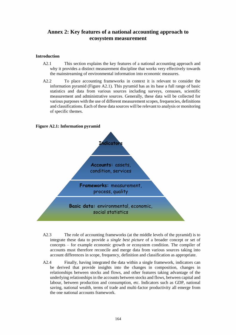
164

Annex 2: Key features of a national accounting approach to

ecosystem measurement

Introduction

A2.1 This section explains the key features of a national accounting approach and

why it provides a distinct measurement discipline that works very effectively towards

the mainstreaming of environmental information into economic measures.

A2.2 To place accounting frameworks in context it is relevant to consider the

information pyramid (Figure A2.1). This pyramid has as its base a full range of basic

statistics and data from various sources including surveys, censuses, scientific

measurement and administrative sources. Generally, these data will be collected for

various purposes with the use of different measurement scopes, frequencies, definitions

and classifications. Each of these data sources will be relevant to analysis or monitoring

of specific themes.

Figure A2.1: Information pyramid

A2.3 The role of accounting frameworks (at the middle levels of the pyramid) is to

integrate these data to provide a single best picture of a broader concept or set of

concepts – for example economic growth or ecosystem condition. The compiler of

accounts must therefore reconcile and merge data from various sources taking into

account differences in scope, frequency, definition and classification as appropriate.

A2.4 Finally, having integrated the data within a single framework, indicators can

be derived that provide insights into the changes in composition, changes in

relationships between stocks and flows, and other features taking advantage of the

underlying relationships in the accounts between stocks and flows, between capital and

labour, between production and consumption, etc. Indicators such as GDP, national

saving, national wealth, terms of trade and multi-factor productivity all emerge from

the one national accounts framework.

Indicators

Accounts: assets, condition, services

Frameworks: measurement, process, quality

Basic data: environmental, economic, social statistics

165

A2.5 The following sub-sections focus on the approach that national accountants

take to providing the single best picture.

Key features of a national accounting approach

A2.6 For those not familiar with the way in which national accountants work

through measurement issues there are two key aspects that should be understood. First,

national accounting approaches generally always commence using data from multiple

sources that has already been collected. National accounting is therefore not focused

on defining survey questions, determining sample sizes, collecting and processing data,

etc. These important tasks are assumed to be completed by experts in specific subject

matter areas, relevant methodologists and those in charge of administrative data.

Ideally, there would be a close relationship between the national accounts compiler and

those collecting the data but this can take time to evolve and in any event the national

accountant will always remain one step removed from the source data.

A2.7 Second, in part as a result of not collecting data, but largely as a result of the

underpinning conceptual framework, national accountants work “from the outside in”.

National accounting is not a “bottom up” measurement approach whereby aggregates

are formed by summing available data. Rather, most effort goes into ensuring that the

estimates that are compiled appropriately reflect the target concept, for example,

economic growth or fixed capital formation or household consumption. Generally, it

will be the case that no single data source can fully encapsulate a single concept and

hence the role of the national accountant is to meld, integrate and otherwise combine

data from multiple sources to estimate the concept as best as possible.

A2.8 Further, on this same point. It is not sufficient to obtain the best estimate of

each concept in isolation. Rather the measurement of each concept must be considered

in the context of the measurement of other concepts following national accounts

identities. Thus, for example, total supply and total use of each product must align.

Ultimately it is the ambition to produce, at a single point in time, the single best picture,

of the concepts in scope of the national accounts framework. This cannot be achieved

by relying on a bottom up strategy where the micro builds neatly to the macro. Instead,

a top down or working from the outside in approach must be applied.

A2.9 Building on these two key aspects there are some related national accounting

compilation principles that should be recognised.

i. The maintenance of time series is fundamental. Perhaps the most important

principle is that in creating the “single best picture” it is not sufficient for each

data point to stand alone in time. Hence changes over time must be considered

as part of the picture. Often national accounts time series extend for over 30 or

40 years and there are few if any data sources that are maintained consistently

over these time frames. Indeed, generally data sources will improve their

methods and coverage over time. Consequently, a key role in national accounts

is linking information from different sources and over time, and hence various

methods may be applied to consistently measure the same concept.

ii. Prices, quantities (volumes) and values are all relevant. While the vast bulk of

the national accounts framework is presented in terms of relationships in value

terms (i.e. in terms of the actual monetary amounts transacted); the most

significant proportion of resources on compiling national accounts are targeted

at decomposing the changes in value between changes in prices or changes in

underlying volumes. Generally, most analysis of the national accounts, e.g.

growth rates, productivity, investment, is conducted in volume terms (i.e. after

166

removing price effects). Again the single best picture ambition requires

balancing these different perspectives at a component and aggregate level.

iii. The need for revisions. Without a time constraint on the integration of data and

the release of results it is likely that national accounts would never be

completed. Given their scope, there is always new information that might be

considered or new methods that might be adopted to refine the single best

picture. National accounting thus works by ensuring the release at regular

intervals of the best picture in the knowledge that it will be revised in due

course when additional information comes to hand.

iv. Accounting is iterative. Fundamentally, the process of integrating data for

accounting is not a single, one-off process. Each time a set of accounts is

compiled different integration issues will arise and will generally only be

resolved through attempting integration, understanding the reasons for

imbalances, and implementing possible solutions. Gradually, a single best

picture emerges. Ideally, resolving these integration issues is a task that

involves both accountants and data supplying areas. Such joint resolution is an

important aspect in mainstreaming different data as part of an overall picture.

A2.10 One overall consequence of a national accounting approach to compilation is

that comparability between different estimates is not assessed primarily on the basis of

method. In the first instance, comparability is based on the extent to which different

estimates accurately reflect the target concept. Indeed, since each national accountant

will be faced with the integration of different source data, a focus on comparability of

methods is likely not a helpful starting point although it must be accepted that not all

methods will produce estimates of equal quality.

A2.11 One benefit of a focus on concepts is that countries will tend to focus their

resources on measuring those aspects within the accounting framework that are of most

relevance to them. For example, in a country in which agriculture is a dominant

activity, resources should be allocated to measurement of this activity. In a different

economic structure, for example a country with a large finance sector, the balance of

resources and the choice of data and methods will and should be different. Since

economic structures changes over time, methods will also need to adapt. The

development of services statistics and associated measurement methods over the past

25 years is a good example of this evolution in compilation approaches even as the

underlying concepts remain stable.

Applying the national accounting approach to ecosystem accounting

A2.12 In most cases, including for the datasets that underpin ecosystem accounting,

the ambition is to generate databases pertaining to a single theme or topic and to

provide the best estimates based on the selected methods and resources available.

While this may well and should involve comparison with other datasets as part of

editing the dataset, it generally does not involve full integration and reconciliation with

other datasets.

A2.13 A national accountant, on the other hand, is not compiling such a dataset but

rather is seeking to undertake the integration. In many respects this is a role that must,

at some point, be undertaken by a data user, analyst or decision maker. That is, at some

point interpretations and judgements are needed concerning data from different sources

that may suggest different trends. Within the scope of macro-economic analysis,

national accountants make such judgements about relative data quality using the rigour

of the national accounting framework. The alternative would be a situation where each

167

economic analyst made their own judgements possibly using varying definitions of

economic aggregates and measurement scope.

A2.14 The application of a national accounting approach within ecosystem

accounting extends this national accounting compilation approach to biophysical and

scientific data. That is, within ecosystem accounting the ambition is to integrate the

various sources of information on ecosystem condition, ecosystem services, economic

production and consumption, to present the single best picture.

A2.15 One consequence is that for ecosystem accounting it is necessary but not

sufficient to have data for a particular ecosystem type or for a selected set of ecosystem

services. Rather, effort must be made to obtain information that permits assessment of

the whole area of interest and full scope of supply of ecosystem services. Certainly it

would be relevant to place most resources into measuring those ecosystems and their

services that are considered most relevant and significant, but this should not detract

from the ambition to measure the whole.

A2.16 In putting national accounts based estimates together it means that data that

may be regarded as of good quality are adjusted to ensure an integrated picture. As

well, since the emphasis is on the measurement of a defined framework, some data

sources may not be used, whatever their quality, since they are not defined following

the required concepts.

A2.17 While these statements are somewhat stark, in practice, a national accounts

approach is very reluctant to ignore any information. Rather, efforts are generally made

to examine all relevant data and, where necessary, make adjustments to concepts to

permit integration.

A2.18 In the area of ecosystem accounting, work is ongoing to define the final

integrated framework. In this context, there remains considerable scope for an active

dialogue between those managing the underlying data sets and those designing the

ecosystem accounting framework. This dialogue is essential for the generation of high

quality information.

Principles and tools of national accounting

A2.19 The focus here is on the main principles and tools that national accountants

apply to ensure coherence in the integration of data from multiple sources. The

following paragraphs present a brief description of the relevant principles. An

extensive discussion of the principles is contained in the SNA 2008 and an extended

overview is provided in SEEA Central Framework.

A2.20 Accounting identities. The accounting system relies on a number of identities

– that is, expressions of relationships between different variables. There are two

relationships of particular importance in ecosystem accounting. First, there is the

supply and use identity in which the supply of a product (or, in this case, an ecosystem

service) must balance with the use of that same product. This identity applies in both

physical and monetary terms. Often information on the supply and use of a product will

be from multiple sources and hence this identity provides a means by which data can

be reconciled.

A2.21 Second, there is the relationship between balance sheets and changes in assets.

This identity is that the opening stock plus additions to stock less reductions in stock

must equal the closing stock. Again, this identity applies in both physical and monetary

terms. Without this identity there would be no particular reason to ensure that observed

changes in ecosystem assets (e.g. through natural growth or extraction) aligned with

168

the series of point-in-time estimates of ecosystem condition that underpin the balance

sheets.

A2.22 Frequency of recording. In order to provide a single best picture across

multiple data sources it is essential that there is a common reference point referred to

in accounting terms as the accounting period. Generally, it is recommended that the

accounting period used across a set of SEEA based accounts is one year. This supports

alignment with economic data that are usually compiled on this periodicity. Flows are

measured such that all activity that takes place during the selected accounting period is

recorded. Stocks are measured at the opening and closing dates of the accounting

period.

A2.23 Commonly, different data sources will have different reference periods and

thus adjustments will be required to allow appropriate integration. For example, flows

may cover a date range that is not aligned with the selected accounting period and/or

stock information will relate to a non-opening or closing period date. Where

adjustments are made these should be made explicit or if no adjustments are made then

the implicit assumptions should be described.

A2.24 For the measurement of some ecosystem characteristics and services the use

of an annual frequency may not be ideal. For example at larger scales changes in

ecosystem extent may only be detectable over periods of three to five years. In the other

direction, measurement of changes in water resources may require sub-annual data to

detect seasonal variation. As appropriate it is relevant to record and present specific

data using these alternative frequencies such that decision making and analysis can be

best supported. At the same time, a single frequency is required for the integration of

all data, including economic data, and it is for this purpose that annual recording is

proposed. This frequency also ensures a regular presentation of ecosystem accounting

data to decision makers and supports the mainstreaming of environmental information

that is a core ambition of the SEEA.

A2.25 In addition to these key principles there are a few common tools and methods

that national accounts apply. These are

A2.26 Benchmarking, interpolation and extrapolation. Among the range of different

data sources there will usually be a particularly high quality source in terms of coverage

and quality. Commonly such a source will provide a benchmark estimate at a point in

time or for a given accounting period. Using this information as a base, it is then

common to use indicators to extrapolate this information to provide more up to date

estimates (a process known as “nowcasting”) and also to interpolate between

benchmarks, for example in cases where the best data are collected every 3 years but

annual estimates are required for accounting purposes. Generally, these techniques are

applied to generate the initial estimates for a particular variable and may be

subsequently adjusted through the balancing and integration process.

A2.27 In some respects these types of benchmarking and interpolation/extrapolation

techniques may be regarded as a form of modelling. The extent to which this is the case

will depend on the sophistication of the technique that is used. Generally, regressions

and the like are not utilised since maintaining these models across the full extent of a

national accounts framework would be very resource intensive. Further, since the

estimates for an individual time series are eventually integrated within a series of

accounting identities it may be difficult to rationalise the statistical advantage of

applying detailed modelling approaches for individual series.

A2.28 Modelling. Where modelling does become more in evidence is when there is a

clear shortage of data for particular variables – i.e. there are no direct estimates or

benchmarks that can be used to provide a starting point. In this case, modelling may be

169

required. An example in standard national accounts is the estimation of consumption

of fixed capital (depreciation) which are commonly derived using the so-called

perpetual inventory model (PIM) that requires estimates of capital formation and

assumptions regarding asset lives and depreciation rates.

A2.29 In the context of ecosystem accounting, the spatial detail required is likely to

considerably increase the need for modelling and this will be new ground for many

national accountants. Chapter 5 of the Technical Recommendations considers the role

of biophysical modelling in ecosystem accounting and the general issue of spatial

imputation where information estimated in one location is applied in other locations.

Such modelling and imputation may be relevant in the measurement of ecosystem

extent, ecosystem condition and ecosystem services. While these may not be traditional

“sources” of information for national accounts type work, there is no particular reason

that such modelled data cannot be directly incorporated. It remains the task of the

accountant to integrate all available data as best as possible. At the same time, a balance

must be found concerning the proportion of data that are modelled within the overall

dataset. Excessive reliance on modelled rather than directly collected data may raise

questions about the accuracy of the information.

A2.30 A general issue that crosses all of the discussion through this section is that of

data quality. Unlike many of the source data that feed into the national accounts it is

not usually possible to give a precise estimate of common measures of data quality

such as standard errors. The melding and synthesis of multiple data sources makes this

task relatively intractable. In the same context it is challenging to measure the

significance of the application of accounting principles on data quality. While clearly

these principles lead to coherence in the final data – it is often unclear how much

adjustment might have been required in order for the coherence to be enforced.

A2.31 Ultimately it will often be the case that accounts are considered of a relatively

good quality if the picture that they present is broadly considered a reasonably accurate

one. This may emerge from consideration of

i. How well the accounts reflect and incorporate data that are considered to

be of high quality.

ii. Commentary by accountants as to the extent of adjustment required (noting

that in a number of situations accounts may be left unbalanced and the size

of the discrepancy may be a measure of quality).

iii. The size of revisions to the estimates where a consistent pattern of large

revisions to initial estimates either up or down would give an indication as

to the relative quality of the source and methods.

iv. The usefulness of the data from the accounts to users. At the end of the day

if the data from the accounts do not support meaningful decision making

or analysis then the quality of the accounts must be questioned.

A2.32 A final area concerns the treatment of uncertainty in accounting contexts.

SEEA EEA Chapter 5 provides an overview of several areas of uncertainty that may

affect information used in ecosystem accounting. By its nature, accounting aims to

provide a single best picture and in this context it would seem to ignore issues of

uncertainty. Three points should be noted. First, to the extent that the inputs into an

accounting exercise are subject to uncertainty then this should be taken into

consideration in the compilation of the accounts themselves. Ideally, degrees of

concern about the data would be the subject of description in the reporting of

accounting outputs. The same holds true for any assumptions that are applied in the

construction of accounting estimates – for example in terms of estimating future flows

of ecosystem services in net present value calculations.

170

A2.33 Second, while not generally undertaken, it would be plausible to consider

publishing some ecosystem accounting aggregates within sensitivity bounds. The

challenge of course is to ensure that a balance in the accounting identities would be

meaningfully maintained but with further consideration of how uncertainty can be

usefully reflected within an accounting context would be welcome.

A2.34 Third, accounting does not provide a model for forecasting future changes in

systems. The national accounts organise information about the composition and

changes in economic activity but do not purport to provide future estimates of

economic growth. Economic models perform this role, generally using time series of

national accounts data.

A2.35 In the same way, ecosystem accounting is not designed to provide a model of

how the ecosystem behaves that can be used to forecast ecological outcomes. It records,

ex post, measures of changes in ecosystem condition and flows of ecosystem services.

How this information might be combined to support estimates of future flows or

changes in condition is a separate issue and likely subject to considerable uncertainties.

This distinction between creating a structured set of information and modelling future

states is often not made in scientific discourse and usually forgotten by economists.

However, it is fundamental to understanding the role that accounting may be able to

play in supporting the mainstreaming of environmental information into decision

making.

A2.36 The inappropriateness of the national accounts as a forecasting model must be

distinguished from the use of future data in the derivation of some national accounting

estimates. A particular example is the use of information on future flows of services in

the measurement of ecosystem capacity and ecosystem asset net present values. While

it is true that net present values require information on future flows, ideally this

information should be obtained from specific data sources, models and expert opinion.

Where such inputs are not available, national accountants will commonly make

assumptions about the future flows (usually based on past history) such that a net

present value can be estimated. However, this is quite different from concluding that

the national accounts framework provides a model that can be used for forecasting.

171

References

Arrow, K. et al. (2012) “Sustainability and the measurement of wealth”, Environmental and

Development Economics, 17: 317-353.

Ajani, J. and P. Comisari (2014) Towards a Comprehensive and Fully Integrated Stock and

Flow Framework for Carbon Accounting in Australia. Australian National University,

Canberra.

Atkinson G. and C. Obst (2017) Defining exchange values for non-market transactions in

ecosystem accounting using environmental economics, May 2017.

Australian Bureau of Statistics (2015). Information paper: An Experimental Ecosystem

Account for the Great Barrier Reef Region. ABS catalogue number 4680.0.55.001, ABS,

Canberra.

Bagstad, K.J., D.J. Semmens, S. Waage and R. Winthrop (2013) A comparative assessment of

decision-support tools for ecosystem services quantification and valuation, Ecosystem

Services, 5: 27–39

Bagstad, K.J., et al. (2014) From theoretical to actual ecosystem services: mapping

beneficiaries and spatial flows in ecosystem services assessments, Ecology and Society,

19:64

Banzhaf, S. and J. Boyd (2012) The architecture and measurement of an ecosystem services

index, Sustainability 4:430-461

Barbier, E. (2013) Wealth accounting, ecological capital and ecosystem services,

Environment and Development Economics, 18(2):133–161

Barton D., et al. (2015) Materials and methods appendix for valuation of ecosystem services

of green infrastructure in Oslo, NINA Report 1115

Bateman, I. J., G.M. Mace, C. Fezzi, G. Atkinson and K. Turner (2011) Economic analysis

for ecosystem service assessment, Environmental and Resource Economics, 48: 177–218

Bordt (2014) Compilation of data, tools and methods, Supporting document to the Advancing

the SEEA Experimental Ecosystem Accounting project, United Nations.

Bordt, M. (2015a) Land and ecosystem condition and capacity, Supporting document to the

Advancing the SEEA Experimental Ecosystem Accounting project, United Nations.

Bordt, M. (2015b) Spatial units, scaling and aggregation, Supporting document to the

Advancing the SEEA Experimental Ecosystem Accounting project. United Nations.

Bordt, M. (2017) Which ecosystems provide which services? In: Bordt, M. (Ed.), Improving

Convergence and Aggregation in National Ecosystem Accounting. University of

Ottawa, Ottawa, Canada Doctoral Thesis. Available

at: https://ruor.uottawa.ca/handle/10393/35826.

Ciais, P., M. Wattenbach, N. Vuichard, P. Smith, S. L. Piao, A. Don, S. Luyssaert, I. A.

Janssens, A. Bondeau, R. Dechow, A. Leip, P. C. Smith, C. Beer, G. R. Van Der Werf, S.

Gervois, K. Van Oost, E. Tomelleri, A. Freibauer and E. D. Schulze (2010) The European

carbon balance. Part 2: croplands, Global Change Biology 16(5): 1409-1428.

Campos, P. And A. Caparrós (2011), RECAMAN PROJECT Mediterranean Monte

Ecosystems Total Income Green Accounting, Presentation at the Expert Meeting on

Ecosystem Accounting, May 2011, European Environment Agency, Copenhagen.

(available at http://unstats.un.org/unsd/envaccounting/seearev/meetingMay2011/lod.htm

Carpenter, S.R., et al. (2010) General Resilience to Cope with Extreme Events, Sustainability,

4(12), 3248-3259; doi:10.3390/su4123248

172

Certain, G. and O. Skarpaas (2011) The Nature Index: A General Framework for

Synthesizing Knowledge on the state of Biodiversity, PLoS ONE, 6: e18930.

CBD (1992) Convention on Biological Diversity, Article 2: Use of terms.

CBD (2003) Interlinkages between biological diversity and climate change, CBD Technical

Series No 10. Secretariat of Convention on Biological Diversity, Montreal.

CBS and WUR (2015) Ecosystem Accounting Limburg Province, the Netherlands. Part I:

Physical supply and condition accounts. Available at: http://www.wur.nl/en/Expertise-

Services/Chair-groups/Environmental-Sciences/Environmental-Systems-Analysis-

Group/Research/Ecosystem-Services-and-Biodiversity/Ecosystem-Accounting.htm

Champ, P. et al. (eds.) (2017) A Primer on Non-market Valuation, 2nd edition Kluwer Academic

Publishing, Dordrecht.

Chapin, F.S. III, et al. (2006) Reconciling carbon-cycle concepts, terminology and methods,

Ecosystems, 9:1041-1050

Cosier P. and J. McDonald (2010) A common currency for building environmental

(ecosystem) accounts, Meeting of the London Group on Environmental Accounting.

Santiago, 25 – 28 October 2010.

Dasgupta, P. S. (2009) The Welfare Economic Theory of Green National Accounts,

Environmental & Resource Economics, 42(1):3–38

Day, B. (2013) An overview of valuation techniques for ecosystem accounting, School of

Environmental Sciences, University of East Anglia, mimeo.

Driver, A., Sink, K.J., Nel, J.L., Holness, S.H., Van Niekerk, L., Daniels, F., Jonas, Z.,

Majiedt, P.A., Harris, L. and Maze, K. (2012) National Biodiversity Assessment 2011:

An assessment of South Africa’s biodiversity and ecosystems. Synthesis report. South

African National Biodiversity Institute & Department of Environmental Affairs, Pretoria.

Edens, B. and L. Hein (2013) Towards a consistent approach for ecosystem accounting,

Ecological Economics, 90:41–52

Ekins, P., et al. (2003) A framework for the practical application of the concepts of critical

natural capital and strong sustainability, Ecological Economics, 44: 165-185

European Commission, International Monetary Fund, Organisation for Economic Co-

operation and Development, United Nations, World Bank (2009) System of National

Accounts 2008, United Nations, New York

Eurostat and OECD (2013) Nutrient budgets: Methodology and handbook, Luxembourg.

FAO (2015) Global Forest Resources Assessment, 2015: How are the World’s Forests

Changing? Rome. Available at: http://www.fao.org/3/a-i4793e.pdf

FAO and United Nations (2016) SEEA Agriculture, Forestry and Fisheries, Draft presented to

the 11th meeting of UNCEEA, 22-24 June, 2016.

FAO and Global Land Cover Network (2009) Land Cover Classification System v.3 (or Land

Cover Meta Language): Design criteria. Rome.

Farley, J, (2008) Valuing Natural Capital: The Limits of Complex Valuation in Complex

Systems, Conference Paper – Economics and Conservation in the Tropics: A Strategic

Dialogue, Jan 31 – Feb 1, 2008. Available from: http://www.rff.org/files/sharepoint/Documents/08_Tropics_Conference/Tropics_Confere

nce_Farley_Valuing%20Natural%20Capital.pdf

Fenichel, E.P. and J.K. Abbott (2014) Natural capital: From Metaphor to measurement,

Journal of the Association of Environmental and Resource Economists, 1(1): 1-27.

173

Freeman, A.M. III, et al. (2013) The Measurement of Environmental and Resource Values:

Theory and Methods, 3rd edition, RFF Press, Washington DC.

Haines-Young R. and M. Potschin (2013) Common International Classification of Ecosystem

Services (CICES), Consultation on version 4, August-December 2012, EEA Framework

Contract No EEA/IEA/09/003

Hamilton, K. and M. Clemens (1999) Genuine savings rates in developing countries, World

Bank Economic Review, Vol 13 (2): 333-356

Harrison, A. (1993) The Draft Handbook and the UNSTAT Framework: Comments. In: Lutz

E (ed) Toward Improved Accounting for the Environment. World Bank, Washington

D.C.

Hein, L. (2014) Guidelines for biophysical modelling and mapping, Supporting document to

the Advancing the SEEA Experimental Ecosystem Accounting project, United Nations.

Hein, L., et al. (2015) Progress and challenges in the development of ecosystem accounting as

a tool to analyse ecosystem capital, Current Opinion in Environmental Sustainability, 14:

86-92

Hein, L., et al. (2016) Defining ecosystem assets for natural capital accounting, PLOS One,

11(11): e0164460, doi:10.1371/journal. pone.0164460

International Integrated Reporting Council (2013), “The international framework”, IIRC,

available at: www.theiirc.org

IUCN (2014) The IUCN Red List of Threatened Species. Version 2014.1.

http://www.iucnredlist.org.

Ivanov, E. (2015) Land accounts and ecosystem extent, Supporting document to the

Advancing the SEEA Experimental Ecosystem Accounting project, United Nations.

Karl, J.W. (2010) Spatial Predictions of Cover Attributes of Rangeland Ecosystems Using

Regression Kriging and Remote Sensing, Rangeland Ecology & Management, 63, Issue

3, May 2010, Pages 335–349

Keith, D.A., Rodríguez, J.P., Rodríguez-Clark, K.M., Nicholson, E., Aapala, K., Alonso, A.,

Bachman, S., Basset, A., Barrow, E.G., Benson, J.S., Bishop, M.J., Bonifacio, R., Brooks,

T.M., Burgman, M.A., Comer, P., Comín, F.A., Essl, F., Faber-Langendoen, D.,

Fairweather, P.G., Holdaway, R.J., Jennings, M., Kingsford, R.T., Lester, R.E., Mac

Nally, R., McCarthy, M.A., Moat, J., Oliveira-Miranda, M.A., Pisanu, P., Poulin, B.,

Regan, T..J., Riecken, U., Spalding, M.D. and Zambrano-Martinez, A. (2013) Scientific

foundations for an IUCN Red List of ecosystems. PLoS ONE, 8(5): e62111.

La Notte, A., J. Maes, S. Dalmazzone, N. Crossman, B. Grizzetti, G. Bidoglio (2017)

Physical and monetary ecosystem service accounts for Europe: A case study for in-stream

nitrogen retention, Ecosystem Services, 23:18-29

La Notte, A., S. Vallecillo, C. Polce, G. Zulian, J. Maes (2017) Implementing an EU system

of accounting for ecosystems and their services: Initial proposals for the implementation

of ecosystem services accounts, EUR28681 EN ; Publications Office of the European

Union, Luxembourg, doi :10.2760/214137, JRC107150

Landers, D. H. and A.M. Nahlik (2013) Final ecosystem goods and services – Classification

system. US Environmental Protection Agency, Office of Research and Development,

Washington, D.C.

Maes, J., A. Teller, M. Erhard, C. Liquete, L. Braat, P. Berry and G. Bidoglio (2013),

Mapping and Assessment of Ecosystems and their Services, An Analytical Framework

for Ecosystem Assessments under Action 5 of the EU Biodiversity Strategy to 2020,

Publications Office of the European Union, Luxembourg.

174

Maynard, S., D. James and A. Davidson (2014) Determining the value of multiple ecosystem

services in terms of community wellbeing: Who should be the valuing agent? Ecological

Economics

Millennium Ecosystem Assessment (2005) Volume I. Ecosystems and human well-being:

Current state and trends. Island Press, Washington, D.C.

Nel, J.L. and A. Driver (2015) National River Ecosystem Accounts for South Africa.

Discussion document for Advancing SEEA Experimental Ecosystem Accounting Project,

October 2015. South African National Biodiversity Institute, Pretoria

Nordhaus, W.D. (2006) “Principles of national accounting for nonmarket accounts”, in

Jorgenson, D. et al. (eds.) A New Architecture for the US National Accounts, Chicago

University Press, Chicago.

Obst, C. and M. Vardon (2014) Recording environmental assets in the national accounts,

Oxford Review of Economic Policy, Vol 30, 126-144.

Obst C., L. Hein, B. Edens (2015). National accounting and the valuation of ecosystem assets

and their services. Environmental and Resource Economics, DOI 10.1007/s10640-015-

9921-1

OECD (2009) Measuring Capital: OECD Manual, second edition, OECD, Paris.

OECD, IMF, ILO, Interstate Statistical Committee of the CIS (2002) Measuring the non-

observed economy: A handbook, OECD, Paris.

Pascual U., et al. (2017) Valuing nature’s contributions to people: the IPBES approach,

Current Opinion in Environmental Sustainability, 26: 7-16

Philips, S. J., R.P. Anderson and R.E. Schepire (2006) Maximum entropy modelling of

species geographic distributions, Ecological modelling, 190: 231-259

Plummer, M. L. (2009) Assessing benefit transfer for the valuation of ecosystem services,

Frontiers in Ecology and the Environment, 7: 38–45. doi:10.1890/080091

Potter, C. S. (1993) Terrestrial ecosystem production: a process model based on global

satellite and surface data, Global Biogeochemical Cycles, 7(4): 811-841

Remme, R. P., M. Schröter and L. Hein (2014) Developing spatial biophysical accounting for

multiple ecosystem services, Ecosystem Services, 10, 6-18

Remme, R.P., B. Edens, M. Schröter and L. Hein (2015) Monetary accounting of ecosystem

services: A test case for Limburg province, the Netherlands. Ecological Economics, 112:

116-128.

Remme, R. P., L Hein and C. van Swaay (2016) Exploring spatial indicators for biodiversity,

Ecological Indicators, 70, pp 232–248

Running, S. W., R. R. Nemani, F. A. Heinsch, M. Zhao, M. Reeves and H. Hashimoto (2004)

A continuous satellite-derived measure of global terrestrial primary production,

BioScience, 54(6): 547-560.

Sbrocchi C., et al. (2015) Evaluation of the Australian Regional Environmental Accounts

Trial, Wentworth Group of Concerned Scientists, Sydney

Schröter, M., D.N. Barton, R.P. Remme and L. Hein (2014) Accounting for capacity and flow

of ecosystem services: A conceptual model and a case study for Telemark, Norway,

Ecological Indicators, 36:539-551

Schröter M., et al. (2015) Lessons learned for spatial modelling of ecosystem services in

support of ecosystem accounting, Ecosystem Services, 13: 64–69

Statistics Canada (2010) Freshwater Supply and Demand in Canada, Human Activity and the

Environment, 16-201-X. Ottawa: Government of Canada.

175

Statistics Canada (2013) Measuring Ecosystem Goods and Services 2013, Human Activity

and the Environment, 16-201-XWE. Ottawa: Government of Canada.

Statistics Canada (2016) The changing landscape of Canadian metropolitan areas, Human

Activity and the Environment. 16-201-X. Ottawa: Government of Canada.

Stoorvogel, Jetse J., Michel Bakkenes, Arnaud J. A. M. Temme, Niels H. Batjes and Ben ten

Brink (2016) S-World: a Global Soil Map for Environmental Modelling, Land

Degradation and Development, doi: 10.1002/ldr.2656.

Sumarga E. and L. Hein (2014) Mapping ecosystem services for landscape planning, the case

of Central Kalimantan, Environmental management, 54: 84-97.

Sumarga E., et al. (2015) Mapping monetary values of ecosystem services in support of

developing ecosystem accounts, Ecosystem Services, 12: 71–83.

TEEB (2010a) The economics of ecosystems and biodiversity, Mainstreaming the economics

of nature. A synthesis of the approach, conclusions and recommendations of TEEB.

Routledge, Oxford, UK.

TEEB (2010b) The economics of valuing ecosystem services and biodiversity (Chapter 5).

Available at: http://www.teebweb.org/wp-content/uploads/2013/04/D0-Chapter-5-The-

economics-of-valuing-ecosystem-services-and-biodiversity.pdf

Turner, D. P., W. D. Ritts, Z. Yang, R. E. Kennedy, W. B. Cohen, M. V. Duane, P. E.

Thornton and B. E. Law (2011) Decadal trends in net ecosystem production and net

ecosystem carbon balance for a regional socioecological system Forest Ecology and

Management, 262(7): 1318-1325.

UK National Ecosystem Assessment (2011) The UK National Ecosystem Assessment:

Synthesis of the key findings. UNEP-WCMC, Cambridge.

UK ONS (2016) Scoping UK Coastal Margin Ecosystem Accounts, Office for National

Statistics, London. Available from:

https://www.ons.gov.uk/economy/environmentalaccounts/methodologies/scopingukcoast

almarginecosystemaccounts

UK ONS (2017) Principles of Natural Capital Accounting, Office for National Statistics,

London. Available from:

https://www.ons.gov.uk/economy/environmentalaccounts/methodologies/principlesofnatu

ralcapitalaccounting

United Nations (1993) Handbook of National Accounting: Integrated Environmental and

Economic Accounting, Interim version. Studies in methods, Series F, No. 61. United

Nations, New York.

United Nations (2012a) International Recommendations for Water Statistics. Statistical

Papers, Series M, No.91. Sales No. 10.XVII.15.

United Nations (2012b) SEEA-Water: System of Environmental-Economic Accounting for

Water. Statistical Papers, Series F, No.100. Sales No. E11.XVII.12.

United Nations (2015) Framework for the Development of Environment Statistics, New

York.

United Nations Statistics Division (2013) System of environmental-economic accounting

2012 – Implementation guide, Draft presented to the London Expert Group on

Environmental-Economic Accounting, November 2013.

United Nations, World Tourism Organisation, European Commission and OECD (2010).

Tourism Satellite Account: Recommended Methodological Framework 2008, Studies in

Methods Series F No 80/ rev1. United Nations, New York.

176

United Nations, European Commission, Food and Agricultural Organization of the United

Nations, International Monetary Fund, Organisation for Economic Co-operation and

Development, The World Bank (2014a) System of Environmental-Economic Accounting

2012 – Central Framework. United Nations, New York

United Nations, European Commission, Food and Agricultural Organization of the United

Nations, Organisation for Economic Co-operation and Development, The World Bank

(2014b) System of Environmental-Economic Accounting 2012 – Experimental

Ecosystem Accounting. United Nations, New York

United Nations, European Union, Food and Agricultural Organization of the United Nations,

Organisation for Economic Co-operation and Development, The World Bank (2017)

System of Environmental-Economic Accounting 2012 – Applications and Extensions.

United Nations, New York.

UNDP (2014) Human Development Report. UNDP, New York.

UNEP (2015) Guidance Manual on Valuation and Accounting of Ecosystem Services for

Small Island Developing States, UNEP, Nairobi.

UNEP-WCMC (2015) Experimental Biodiversity Accounting as a component of the System

of Environmental-Economic Accounting Experimental Ecosystem Accounting (SEEA

EEA). Supporting document to the Advancing the SEEA Experimental Ecosystem

Accounting project. United Nations. Available from:

http://wcmc.io/SEEA_EEA_Bio_Accounting

UNEP-WCMC (2016) Exploring approaches for constructing Species Accounts in the context

of the SEEA EEA. Available at: http://wcmc.io/Species_Accounting

UNU-IHDP and UNEP (2014) Inclusive Wealth Report, 2014, Measuring Progress Toward

Sustainability. Cambridge University Press, Cambridge, UK

UNWTO (2017) Statistical Framework for Measuring Sustainable Tourism, Preliminary draft

prepared for the 6th International Conference on Tourism Statistics, Manila, Philippines,

June 2016. Available from:

https://custom.cvent.com/E5C28A0D212A415D9AD3C8B699EBC072/files/121578cbeb

154e25a9f124813a3e754e.pdf

United States Environmental Protection Agency (US EPA) (2015) National Ecosystem

Services Classification System (NESCS): Framework design and policy application.

EPA-800-R-15-002, Washington DC, USEPA.

Vanoli, A. (1995) Reflections on Environmental Accounting Issues, Review of Income and

Wealth, 41(2):113-137

Vardon, M. (2014a) Water and ecosystem accounting, Supporting document to the Advancing

the SEEA Experimental Ecosystem Accounting project, United Nations.

Vardon, M. (2014b) Carbon and ecosystem accounting, Supporting document to the

Advancing the SEEA Experimental Ecosystem Accounting project. United Nations.

Victorian Department of Sustainability and Environment (2013) Victorian experimental

ecosystem accounts, Victorian Government, East Melbourne, Australia.

WAVES-Philippines (2016) Pilot Ecosystem Account for Southern Palawan, WAVES

Technical Report, November, 2016. Available from:

https://www.wavespartnership.org/sites/waves/files/kc/WB_Southern%20Palawan%20Te

ch%20Report_FINAL_Nov%202016.pdf

Weber, J-L. (2011) An experimental framework for ecosystem capital accounting in Europe,

EEA Technical Report No 13/2011, ISSN 1725-2237, European Environment Agency,

Copenhagen, Denmark.

177

Weber, J-L (2011) Recording ecological debts in the national accounts. Research paper

Available from:

https://www.google.com.au/url?sa=t&rct=j&q=&esrc=s&source=web&cd=14&ved=0ah

UKEwjv9o32hrPWAhUDNJQKHUVCAqsQFghnMA0&url=http%3A%2F%2Fprojects.

eionet.europa.eu%2Fleac%2Flibrary%2Fcube%2Frecording_ecological%2Fdownload%2

Fen%2F1%2FRecording%2520ecological%2520debts%2520in%2520the%2520national

%2520accounts_edited.doc&usg=AFQjCNFO2nC1JXcZpuIHobZWkdhEzcQRIg

Weber, J-L. (2014a) Ecosystem Natural Capital Accounts: A Quick Start Package, Technical

series No. 77. Secretariat of the CBD. Montreal

Weber, J-L. (2014b) Mauritius case study of experimental ecosystem natural capital accounts:

Methodology and preliminary results. Indian Ocean Commission, Mauritius.

Willemen, L., et al. (2015) Best Practices for Mapping Ecosystem Services, Ecosystem

Services, Volume 13: 1–5

World Bank (2011) The Changing Wealth of Nations, World Bank, Washington D.C.

World Bank (2014) Designing Pilots for Ecosystem Accounting, WAVES, World Bank,

Washington.

World Bank (2017) Better Policy through Natural Capital Accounting: Stocktaking and Ways

Forward, 7th WAVES Annual Partnership Meeting Edition, June 2017. Available from:

https://www.wavespartnership.org/sites/waves/files/kc/Policy%20forum%20papers%20%

281%29.pdf

World Wildlife Fund (2014) Living Planet Report. WWF/ESA.