Segmentation of Large Periapical Lesions toward Dental Computer-

Aided Diagnosis in Cone-Beam CT Scans

Steven Rysavya, Arturo Flores

a, Reyes Enciso

b, Kazunori Okada

a

aSan Francisco State University, 1600 Holloway Ave., San Francisco, CA USA 94132 bUniversity of Southern California, 925 West 34

th St., Los Angeles, CA USA 90089

ABSTRACT

This paper presents an experimental study for assessing the applicability of general-purpose 3D segmentation algorithms

for analyzing dental periapical lesions in cone-beam computed tomography (CBCT) scans. In the field of Endodontics,

clinical studies have been unable to determine if a periapical granuloma can heal with non-surgical methods. Addressing

this issue, Simon et al. recently proposed a diagnostic technique which non-invasively classifies target lesions using

CBCT. Manual segmentation exploited in their study, however, is too time consuming and unreliable for real world

adoption. On the other hand, many technically advanced algorithms have been proposed to address segmentation

problems in various biomedical and non-biomedical contexts, but they have not yet been applied to the field of dentistry.

Presented in this paper is a novel application of such segmentation algorithms to the clinically-significant dental

problem. This study evaluates three state-of-the-art graph-based algorithms: a normalized cut algorithm based on a

generalized eigen-value problem, a graph cut algorithm implementing energy minimization techniques, and a random

walks algorithm derived from discrete electrical potential theory. In this paper, we extend the original 2D formulation of

the above algorithms to segment 3D images directly and apply the resulting algorithms to the dental CBCT images. We

experimentally evaluate quality of the segmentation results for 3D CBCT images, as well as their 2D cross sections.

The benefits and pitfalls of each algorithm are highlighted.

Keywords: Segmentation, Dental CAD

1. INTRODUCTION

A periapical cyst is an inflamed area surrounding the roots of a tooth with associated infected and dying pulp. A

granuloma is a mass of chronically inflamed granulation tissue resulting from irritation following pulp disease or

endodontic treatment. Granulomas often heal independently while periapical cysts can continue to cause further clinical

problems. Differentiating between these two types of lesions is difficult.

No method exists in Endodontics, the branch of dentistry specializing in dental pulp, to non-invasively and

accurately differentiate periapical cysts from granulomas. Currently, a biopsy is performed and the tissue is analyzed to

conclude whether the region is a periapical cyst or a granuloma. Unfortunately the procedure is surgical once the biopsy

is taken, so the possibility for the granuloma to heal by itself is lost. Furthermore, the patient is subjected to unnecessary

pain and discomfort from the surgical procedure, as well as potential complications such as infection.

1.1 Previous Study

A team of researchers at the University of Southern California (USC) have proposed a new technique1 to non-

surgically classify a target lesion using 3D cone-beam computed tomography (CBCT). Their technique consisted of

using the lowest and highest gray value measurement in the lesion area, as well as the lowest gray value measurement at

the center of the lesion above the root, to differentiate between cysts and granulomas. Of the 17 lesions analyzed, 13 of

the CBCT diagnosis coincided with the biopsy diagnosis. In four cases, the CBCT diagnosis classified the lesion as a

cyst, while the biopsy diagnosis classified the lesion as a granuloma. Upon closer review of the comments in the biopsy

diagnosis reports for these four cases, they suggested that the CBCT diagnosis may be more accurate.

USC's study provides a proof of concept that CBCT is an effective tool for differentiating between cysts and

granulomas. However, the gray value measurements were taken by manually sampling a number of 3D points within a

lesion via visual inspection. Such a purely manual procedure is prone to human error and labor-intensive, making it

unsuitable for real world deployment.

1.2 Dental Computer-Aided Diagnosis

Computer-Aided Diagnosis (CAD) has made a significant impact in various clinical areas, such as differential

diagnosis of breast tumors,2 and diagnosis of pulmonary nodules

3 to name a few. Such CAD systems have shown

promising results in providing a reliable second opinion and often preventing misdiagnosis.4 However, CAD in the field

of dentistry is still in its early stages. While previous attempts to apply CAD in dentistry exist,5,6,7 this remains an

understudied field. Our approach is to transfer the advanced state-of-the-art CAD techniques into the domain of

dentistry where there are keen demands for such advanced diagnostic solutions.1 Overall, we aim to develop a machine

learning-based system for classifying the periapical lesions in our specific dental context described above. Particularly,

this study focuses on the lesion segmentation which serves as a preprocess of such a classification system. The accurate

3D lesion segmentation offers an effective way to characterize intensity-based features that are inputs to the overall

system.

This paper is organized as follows. We begin with an introduction to our overall dental CAD system and provide

an overview of the three graph-based segmentation algorithms evaluated in this study. In Section 3 we experimentally

evaluate the segmentation algorithms as applied to both 2D cross-sections of DICOM scans as well as full 3D DICOM

scans produced by dental CBCT. Section 4 concludes this contribution.

2. METHODS

Our overall CAD system consists of two stages. In the first stage, a segmentation algorithm is applied to the

CBCT images to determine the region of interest (segmentation stage). This region of interest is then subjected to a

classification algorithm, resulting in a diagnosis (classification stage). This paper focuses on the segmentation stage.

Three state-of-the-art graph based algorithms are evaluated and applied in this paper: a normalized cut algorithm,8

a graph cut algorithm,9 and a random walks algorithm.

10 These are chosen for the successful segmentation results

produced in other applications as well as the variability in the respective approaches. The segmentation algorithms have

been modified from using 2D images as input to 3D DICOM scans.

2.1 Definition and Terminology

A 3D DICOM scan is composed of sequential stack of 2D images. In order to apply the segmentation algorithms,

the DICOM scan is represented as a 3D graph G = (V, W) as follows: Each graph node I is represented by a voxel i,

where V = {1,2, … , N} and N is the number of nodes in the graph. W is the set of edge weights formed between all

nodes i and j, where i,j ∈V. Weights represent the contrast between intensities of two nodes i and j, the calculation

being dependent upon the weighting function specific to each segmentation algorithm.

Each segmentation algorithm partitions the graph G into two disjoint sets A and B, A∪ B = V, A∩ B =φ , by cutting edges connecting the two sets. The nodes within sets A and B are assigned binary values 1 and 0 respectively to

produce a segmentation mask corresponding to the original DICOM scan.

2.2 Segmentation Algorithms

2.2.1 Normalized Cut

The normalized cut algorithm maximizes similarities between voxels while simultaneously minimizes

dissimilarity between voxels.8 This theoretically increases the quality of the segmentation by labeling closely related

voxels together and applying a different label to unrelated voxels. The algorithm performs an automatic segmentation

without manual seeding provided the number of segments and specification of weighting parameters.

The normalized cut problem is NP-complete, even for the special case of grid-based graphs. Shi and Malik show

that the minimization problem becomes tractable when relaxed to include real values.2 By expressing the normalized cut

problems in terms of a Rayleigh quotient,11 the solution can be formulated as a standard eigen-value problem,

xx λ=−−

2

1

2

1

)( DWDD , (1)

where D is a diagonal NxN matrix with d(i) =∑ jjiw ),( along its diagonal and W is an NxN affinity matrix where

W(i,j) = wij. When W is a real symmetrical matrix, as in normalized cut, the real valued solution is the second smallest

eigenvector.11 Subsequent eigenvectors also contribute to the segmentation although the approximation error increases

rapidly due to the relaxing of the discrete value constraint.

Application of this algorithm on a 3D DICOM scan required the generation of a large, sparse weighted 2D graph

using the original weighting algorithm proposed by Shi and Malik:

<−−

−−=

−−

otherwise

rXXifeFF

w

jix

XX

I

ji

ij

ji

0

*2)()(

2

2

2)()(

2

2

2)()(

σ

σ

,

(2)

where F represents the voxel intensity value, X signifies the voxel location, and r is the distance threshold for calculating

voxel weights. Since W is sparse and the solution only requires the top eigenvectors with minimal precision, the

Lanczos method is applied to efficiently obtain the eigenvector solutions.8

2.2.2 Graph Cut

The graph cut algorithm segments images by using energy minimization techniques.9 Relationships between

voxels that do not vary smoothly (have dissimilar intensities) are assigned high energy values while relationships

between similar voxels (have similar intensities) are assigned low energy values. Ideally the proper segmentation

corresponds to a minimum cut, where a graph cut is defined by

∑∈∈

=BjAi

jiwBAcut,

),(),( . (3)

The minimum cut is equivalent to the minimum energy of the graph. Similar to the normalized cut algorithm, the

graph cut algorithm is automatic, provided an automatic initial labeling using a method such as k-means clustering. The

initial labeling can also be user-defined, allowing for a semi-automatic segmentation.

The graph cut algorithm is NP-hard. Boykov et al. provides two approximation algorithms to overcome this

problem: the α-β swap and the α expansion. Both algorithms re-label a large numbers of voxels simultaneously,

allowing for a much faster computation that still falls within a known factor of the global minimum energy. A max-flow

algorithm is also incorporated to speed the computation time of the graph cut algorithm.12,13

2.2.3 Random Walks

The random walks algorithm segments images using electrical circuit theory.10 User-defined seed points are

required for the initialization of this semi-automatic algorithm. Each seed is sequentially assigned a value of one, while

all other seeds on are assigned zero. The electrical potential from each pixel to each seed point is iteratively calculated

based on the intensity of the relationship. Finally, each pixel is assigned to each seed point for which its potential is the

highest. Unlike the normalized cut and graph cut algorithms, this problem is computable in polynomial time, meaning

heuristics are not used for solving this problem.

Weights are defined by the original equation presented by Grady as

))((2

ji gg

ij ew−−= β

, (4)

where g represents the voxel intensity and β is the only free parameter in the algorithm. Treating this as a combinatorial

Dirichlet problem results in a sparse, symmetric, positive-definite system of equations.10 Solving the system of

equations using LU decomposition is possible for small images, but the size of the DICOM scans precludes the approach

in this context. Instead an iterative solver is applied to solve the Dirichlet boundary problem.

2.3 3D Extension

All three algorithms were originally formulated to segment input graphs in a 2D domain. We modified these

algorithms to segment 3D input graphs. The normalized cut algorithm was extended to compare each voxel to other

voxels contained in the 3D volume within the specified threshold distance r. The affinity matrix W remains 2D,

however, and the Lanczos method is still applicable. The graph cut algorithm requires that labels be applied to all voxels

within the 3D image. Edges interconnecting the nodes between each 2D slice were taken into account when finding the

minimum energy of the system, but the energy minimization is done in same way.

The random walk algorithm uses a 4-connected lattice for the electrical potential calculations on 2D data. A 4-

connected lattice is defined by edges from a single node to its immediate perpendicular neighbors. For 3D data, we must

use a 6-connected lattice. A 6-connected lattice also is defined by edges from each node to its immediate perpendicular

neighbors in its 2D plane, with two additional edges to its perpendicular neighbors in the third dimension.

3. EXPERIMENTS

Here we present qualitative experiments for the comparison of the three segmentation algorithms. Figures 3-5

demonstrate the segmentation algorithms as performed on periapical lesions. Each algorithm is applied to a granuloma,

a cyst, and a lesion where the CBCT diagnosis differed from the biopsy diagnosis in the previous study. Figure 3

illustrates the segmentations applied to 2D cross-sections of the DICOM scans. Figure 4 illustrates the segmentations

applied to full 3D DICOM scans. Figure 5 illustrates the random walks segmentations applied to all 17 lesions.

3.1 Data

Data consisting of 17 CBCT DICOM format images of periapical lesions has been provided by USC School of

Dentistry. Each CBCT image was captured using the NewTom 3G at USC. The sharing of this anonymous data was

approved by the Institutional Review Board of USC. Each lesion underwent a histological biopsy and was diagnosed as

either a cyst or granuloma by certified histologists. This dataset contains 7 cyst cases and 10 granuloma cases according

to the biopsy diagnosis.

The CBCT images are stored in the DICOM format and have also been converted for use in MATLAB. A

MATLAB cross-section viewer is used to display the intensity values for each slice of the 3D CBCT image. Intensity

values are inconsistent between CBCT scan instances because the dental cone-beam scanner adoptively shifts radiation

in order to minimize radiation dosage to patients. Thus simple intensity-thresholding is not a viable option for our

segmentation task. Furthermore, the morphology of the periapical lesions can vary. As can be seen in Figure 1, it is

non-trivial to visually segment the lesions.

Fig. 1. Illustrative example of periapical lesions. The cross-hairs denote the center of the lesion. The left three are granulomas, while

the right three are cysts. Visually, they are hard to differentiate.

3.2 Segmentation Results

3.2.1 Normalized Cut

Normalized cut segmentations of a 2D cross-section of periapical lesions are illustrated in Figure 3d-f. Figure 3d

shows cuts corresponding to the second and third eigenvectors of the generalized eigen-value system while Figure 3e

shows cuts corresponding to the second through sixth eigenvectors. The subsequent eigenvectors do not provide useful

segmentation information for these lesions. Figure 3f emphasizes the segmentation using a higher number of

eigenvectors. Figures 4d-f similarly show the normalized cut algorithm as applied to 3D input.

Shi and Malik specify that additional user interaction will be required to correctly label the final segmentation into

two disjoint sets.8 Visual inspection confirms this as some cuts occur outside the boundary of the lesion, such as those in

Figure 3f. Figure 3e exemplifies a typical example of periapical lesion where an implied boundary is visually apparent

yet none of the top eigenvectors segment the images along this weak boundary. Without a cut along the boundary of the

lesion, a complete segmentation of the lesion is not possible by the normalized cut algorithm without additional user

input. Although only three examples are presented for each 2D and 3D cases, these results are representative for all 17

cases.

3.2.2 Graph Cut

Figures 3g-i show the graph cut algorithm applied to 2D cross-sections of periapical lesions. K-means clustering

of the voxel intensity is used as an initial condition for this algorithm. The variation in the initial cluster has minimal

impact on the final segmentation. The final segmentation is virtually identical for α expansion and α-β swap moves. All

figures depicting graph cuts in this contribution consequently use α expansion moves.

Like the normalized cut algorithm, the graph cut algorithm cuts the images closely along the edges of differing

intensity values. Unlike normalized cut, however, graph cut assigns the same label to multiple regions. Like the

normalized cut algorithm, weak lesion boundaries are not always segmented with this algorithm. Figures 4g-i show the

graph cut results off the 3D DICOM scan, which perform similarly to the 2D cross-section segmentations. These results

are representative of all 17 cases provided by USC.

3.2.3 Random Walks

Figures 3j-l illustrate the segmentation of 2D cross-sections produced by the random walks algorithm. Seed points

were manually applied to get these segmentations. Due to the noise of the data, the segmentation varies slightly with the

choice of these seed points. Additional strategically placed seed points increase the quality of segmentation but require

much more user interaction. As can be seen in Figure 3k, the weak edge of the lesion is cut by random walks.

The 3D segmentations as shown in Figures 4j-l are more consistent with random walks due to the way the seed

points are defined. A user-specified center, inner radius and outer radius define two concentric spheres of seed points.

The inner sphere border represents the object seed points and has a radius such that all of the seeds lie inside the lesion

area. The outer sphere border represents the background seed points and has a radius such that all of the seeds lie

outside of the lesion. Variance in these radii does not have a significant impact on the segmentation. Figure 5 illustrates

segmentations produced by the random walks algorithm on all 17 periapical lesions.

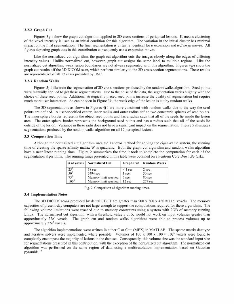
3.3 Computation Time

Although the normalized cut algorithm uses the Lanczos method for solving the eigen-value system, the running

time of creating the sparse affinity matrix W is quadratic. Both the graph cut algorithm and random walks algorithm

have a near linear running time. Figure 2 summarizes the time it took to complete the computation for each of the

segmentation algorithms. The running times presented in this table were obtained on a Pentium Core Duo 1.83 GHz.

# of voxels Normalized Cut Graph Cut Random Walks

253 38 sec < 1 sec 2 sec

503 2494 sec 1 sec 30 sec

753 Memory limit reached 6 sec 80 sec

1003 Memory limit reached 12 sec 277 sec

Fig. 2. Comparison of algorithm running times.

3.4 Implementation Notes

The 3D DICOM scans produced by dental CBCT are greater than 500 x 500 x 450 ≈ 11e7 voxels. The memory

capacities of present-day computers are not large enough to support the computations required for these algorithms. The

following volume limitations were reached due to memory constraints using a system with 2GB of memory running

Linux. The normalized cut algorithm, with a threshold value r of 5, would not work on input volumes greater than

approximately 22e4 voxels. The graph cut and random walks algorithms were able to process volumes up to

approximately 22e5 voxels.

The algorithm implementations were written in either C or C++ (MEX) in MATLAB. The sparse matrix datatype

and iterative solvers were implemented where possible. Volumes of 100 x 100 x 100 ≈ 10e6 voxels were found to

completely encompass the majority of lesions in the data set. Consequently, this volume size was the standard input size

for segmentations presented in this contribution, with the exception of the normalized cut algorithm. The normalized cut

algorithm was performed on the same region of data using a multiresolution implementation based on Gaussian

pyramids.14

(a)

(b)

(c)

(d)

(e)

(f)

(g)

(h)

(i)

(j)

(k)

(l)

Fig. 3. This figure illustrates examples of the three graph-based segmentation algorithms as applied to 2D cross-sections of 3D

DICOM dental CBCT scans. The first row shows the original image. Each subsequent row corresponds to a segmentation

algorithm: the second row depicts the normalized cut segmentations, the third row depicts the graph cut segmentations, and

the last row depicts the random walks segmentation. Each column corresponds to a type of lesion: the first column represents

a granuloma, the second column represents a cyst, and the third column represents a lesion that was classified as a cyst by

Simon’s technique and a granuloma by the biopsy diagnosis.

(a)

(b)

(c)

(d)

(e)

(f)

(g)

(h)

(i)

(j)

(k)

(l)

Fig. 4. This figure illustrates examples of the three graph-based segmentation algorithms as applied to 3D DICOM dental CBCT

scans. The first row shows the original image. The second row depicts the normalized cut segmentations, the third row

depicts the graph cut segmentations, and the last row depicts the random walks segmentation. Each column corresponds to a

type of lesion: the first column represents a granuloma, the second column represents a cyst, and the third column represents a

lesion that was classified as a cyst by Simon’s technique and a granuloma by the biopsy diagnosis. The normalized cut

displays a thicker segmentation line due to artifacts from the Gaussian pyramid enlargment process.

Fig. 5. This figure illustrates the segmentations produced by the random walks algorithm on the remaining cases provided by USC.

4. CONCLUSIONS

We have qualitatively compared the three segmentation algorithms with 3D DICOM dental CBCT scans. The

normalized cut algorithm shows good edge detection for strong edges. However, it does not find weak edges and fails to

fully close the lesion area, resulting in an incomplete segmentation. Additionally, the time complexity for this algorithm

is much higher than the other two algorithms.

The graph cuts algorithm shows good edge detection in 2D. Further refinement is needed to achieve comparable

results in 3D. This algorithm may perform better by incorporating a distance metric based on the center position of the

periapical lesion. Combining intensity and distance metrics may yield a segmentation that is closer to the ground truth

than the current results.

The random walks algorithm does not perform edge detection as well as the normalized cut or graph cut

algorithms. In certain cases, the segmentation leaves out portions of the lesion. A clear example is presented in the top

right cross-section of Figure 3h. However, this algorithm consistently produces a fully closed lesion volume completely

encompassed by the lesion boundary whereas the other two do not. This is a critical requirement for the classification

stage of the overall CAD system. In this respect, this algorithm has the best performance.

As our future work, we plan to develop the classification stage on the segmentations produced by the algorithms

presented in this paper. The classification of the periapical lesions is expected to show significant improvement over the

previous study with the automatic and semi-automatic segmentations. These results are planned to be validated by the

dental experts at USC for further clinical studies.

5. ACKNOWLEDGMENTS

The authors would like to thank the USC school of dentistry for providing the data. Funding for this project has been

provided by the 2006 CSU faculty-student collaborative research seed grant and by the Center for Computing for Life

Sciences at San Francisco State University.

REFERENCES

[1] Simon JHS, Enciso R, Malfaz JM, Roges R. “Differential Diagnosis of Large Periapical Lesions Using Cone-Beam

Computed Tomography Measurements and Biopsy”, Journal of Endodontics 32(9), 833-837 (2006).

[2] Huang Y, Wang K, Chen D. "Diagnosis of Breast Tumors with Ultrasonic Texture Analysis using Support Vector

Machines", Clinical Imaging 29(3), 164 (2006).

[3] Kawata Y, Niki N, Ohmatsu H, Kakinuma R, Mori K, Eguchi K, Kaneko M, Moriyama N, Kusumoto M,

Nishiyama H. “Computer Aided Differential Diagnosis of Pulmonary Nodules Using Curvature Based Analysis”, In

Proceedings of the 10th International Conference on Image Analysis and Processing, 470 (1999).

[4] Doi K, “Diagnostic Imaging over the Last 50 Years: Research and Development in Medical Imaging Science and

Technology”, Phys. Med. Biol. 51(13), R5-R27 (2006).

[5] Li S, Fevens T, Krzyzak A, Jin C, Li S., “Toward Automatic Computer Aided Dental X-ray Analysis Using Level

Set Method”, Pattern Recognition 40(10), 2861-2873 (2007).

[6] Trope M, Pettigrew J, Petras J, Barnett F, Tronstad L. “Differentiation of Radicular Cyst and Granulomas using

Computerized Tomography”, Dental Traumatology 5(2), 69-72 (1989).

[7] Cotti E, Campisi G, Ambu R, Dettori C. “Ultrasound Real-Time Imaging in the Differential Diagnosis of Periapical

Lesions”, International Endodontic Journal 36(8), 556-563 (2003).

[8] Shi J, Malik J. "Normalized Cuts and Image Segmentation." IEEE Transactions on Pattern Analysis and Machine

Intelligence 22(8), 888-905 (2000).

[9] Boykov Y, Veksler O, Zabih R. "Fast Approximate Energy Minimization via Graph Cuts." IEEE Transactions on

Pattern Analysis and Machine Intelligence 23(11), 1222-1239 (2001).

[10] Grady L, "Random Walks for Image Segmentation." IEEE Transactions on Pattern Analysis and Machine

Intelligence 28(11), 1-17(2006).

[11] Golub G, Van Loan C. [Matrix Computations], John Hopkins Press, Baltimore and London, 408-410 (1996).

[12] Boykov Y, Kolmogorov V, “An Experimental Comparison of Min-Cut/Max-Flow Algorithms for Energy

Minimization in Vision”, In IEEE Transactions on Pattern Analysis and Machine Intelligence 26(9), 1124-1137

(2004).

[13] Kolmogorov V, Zabih R, “What Energy Functions can be Minimized via Graph Cuts?”, IEEE Transactions on

Pattern Analysis and Machine Intelligence 20(12), 147-159 (2004).

[14] Adelson E, Anderson C, Bergen J, Burt P, Ogden J., “Pyramid Methods in Image Processing”, RCA Engineer 29(6),

33-41 (1984).