Segmentation

What is Image Segmentation? There are many definitions:

Segmentation subdivides an image into its constituent regions or objects ( Gonzales, pp567)

Segmentation is a process of grouping together pixels that have similar attributes ( Efford , pp250)

Image Segmentation is the process of partitioning an image into non-intersecting regions such that each region is homogeneous and the union of no two adjacent regions is homogeneous ( Pal, pp1277)

What is Image Segmentation

Segmentation is typically associated with pattern recognition problems. It is considered the first phase of a pattern recognition process and is sometimes also referred to as object isolation.

Image Segmentation

Feature

Extraction Classification

Input Image

Object Image

Feature VectorObject Type

What do we mean by “labeling” an image?

When we say w e ”extract “ an object in an image , we mean that we identify the pixels that make it up. To express this information , we create an array of the same size as the original image and we give to each pixel a label. All pixels that make up the object are given the same label . The label is usually a number, but it could be anything: a letter, or color. Often label images are also referred to as classified images as they indicate the class to which each pixel belongs.

Why segmentation is difficult ?

It can be difficult for many reasons:

•Non- uniform illumination

•No control of the environment

•Inadequate model of the object of interest

•Noise

Why segmentation is useful ?

Segmentation algorithms have been used for a variety of applications. Some examples are :

•Optical character recognition(OCR)

•Automatic Target Acquisition

•Colorization of Motion Pictures

•Detection and measurement of bone, tissue, etc, in medical images.

How can we divide an image into uniform regions ?

Segmentation techniques can be classified as either contextual or non-contextual .

Non-contextual techniques ignore the relationships that exist between features in an image; pixels are simply grouped together on the basis of some global attribute, such as grey level.

Contextual techniques, additionally exploit the relationships between image features. Thus, a contextual technique might group together pixels that have similar grey levels and are close to one another .

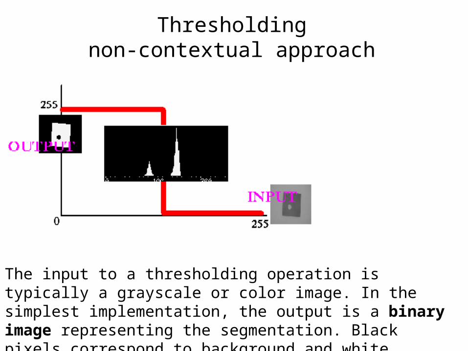
Thresholding non-contextual approach

The input to a thresholding operation is typically a grayscale or color image. In the simplest implementation, the output is a binary image representing the segmentation. Black pixels correspond to background and white pixels correspond to foreground (or vice versa).

Threshopding of pixel grey level ( Basic Global Thresholding)

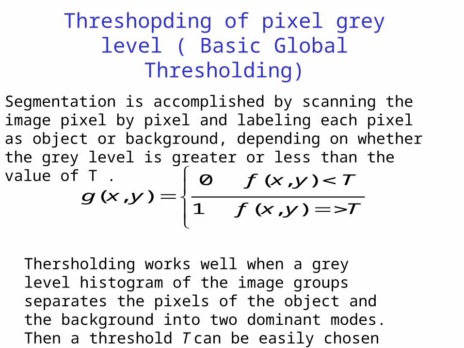
Segmentation is accomplished by scanning the image pixel by pixel and labeling each pixel as object or background, depending on whether the grey level is greater or less than the value of T .

Tyxf

Tyxfyxg

),(1

),(0),(

Thersholding works well when a grey level histogram of the image groups separates the pixels of the object and the background into two dominant modes. Then a threshold T can be easily chosen between the modes.

Picking the threshold is the hard part

• Human operator decided the threshold

• Use mean gray level of the image

• A fixed proportion of pixels are detected ( set to 1) by the thresholding operation

•Analyzing the histogram of an image

Basic Global Thresholding

Figure 1 A) shows a classic bi-modal intensity distribution. This image can be successfully segmented using a single threshold T1. B) is slightly more complicated. Here we suppose the central peak represents the objects we are interested in and so threshold segmentation requires two thresholds: T1 and T2. In C), the two peaks of a bi-modal distribution have run together and so it is almost certainly not possible to successfully segment this image using a single global threshold

Basic Global Thresholding

The same approach can be used with more than one treshold value.For example, for threshold T1 and T2, any point which satisfies the relation T1<f(x,y) <T2 would be labeled as an object point and all others would be labeled background points.

In general this technique is less reliable than a single variable threshold. This is because it often difficult to establish multiple thresholds to effectively isolate the region of interest especially when the number of modes in the corresponding histogram is high.

Basic Global and Local Thresholding

Thresholding may be viewed as an operation that involves tests against a function T of the form:

T = T[x,y,p(x,y),f(x,y)]

Where f(x,y) is the gray level , and p(x,y) is some local property.

Simple tresholding schemes compare each pixels gray level with a single global threshold. This is referred to as Global Tresholding.

If T depends on both f(x,y) and p(x,y) then this is referred to a Local Thresholding.

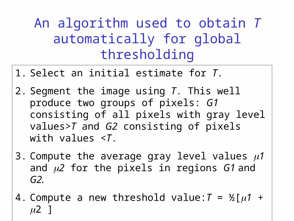
An algorithm used to obtain T automatically for global thresholding

1. Select an initial estimate for T.

2. Segment the image using T. This well produce two groups of pixels: G1 consisting of all pixels with gray level values>T and G2 consisting of pixels with values <T.

3. Compute the average gray level values 1 and 2 for the pixels in regions G1 and G2.

4. Compute a new threshold value:T = ½[1 + 2 ]

5. Repeat step 2 through 4 until the difference in T in successive iterations is smaller than a predefined parameter To.

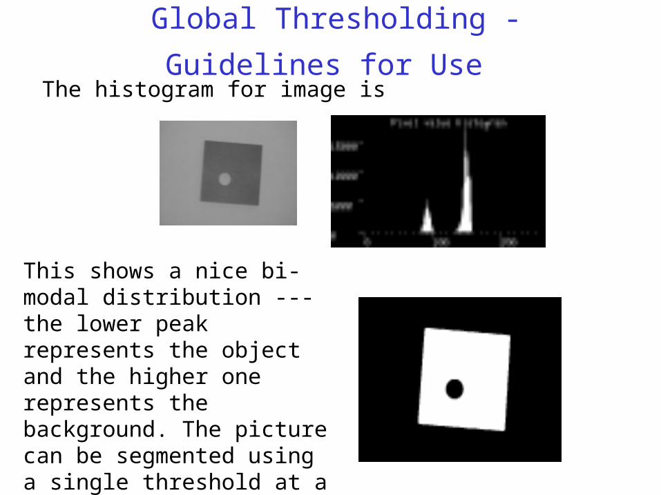
Global Thresholding - Guidelines for Use  The histogram for image is

This shows a nice bi-modal distribution --- the lower peak represents the object and the higher one represents the background. The picture can be segmented using a single threshold at a pixel intensity value of 120. The result is shown in

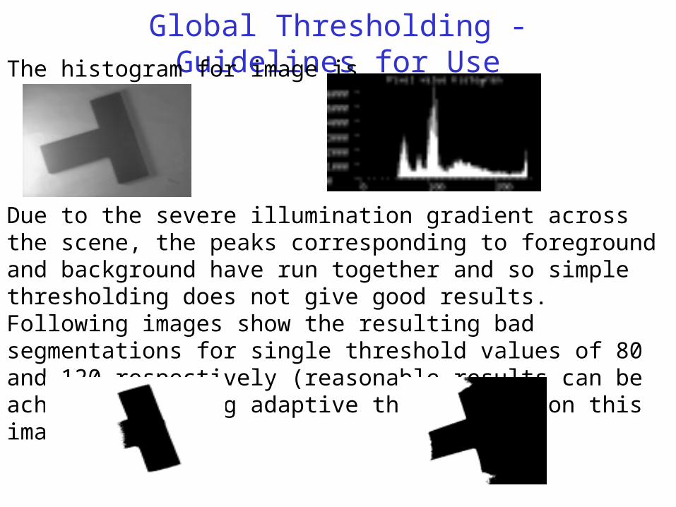
Global Thresholding - Guidelines for UseThe histogram for image is

Due to the severe illumination gradient across the scene, the peaks corresponding to foreground and background have run together and so simple thresholding does not give good results. Following images show the resulting bad segmentations for single threshold values of 80 and 120 respectively (reasonable results can be achieved by using adaptive thresholding on this image).

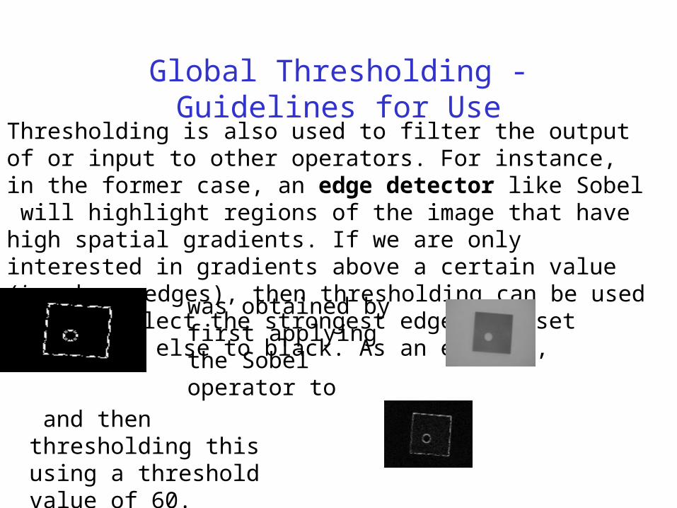
Global Thresholding - Guidelines for UseThresholding is also used to filter the output of or input to other operators. For instance, in the former case, an edge detector like Sobel will highlight regions of the image that have high spatial gradients. If we are only interested in gradients above a certain value (i.e. sharp edges), then thresholding can be used to just select the strongest edges and set everything else to black. As an example,

was obtained by first applying the Sobel operator to

 and then thresholding this using a threshold value of 60.

Use of Boundary Characteristics for Histogram Improvement and Local

Thresholding

From the privies discussion , an indication of whether a pixel is on an edge may be obtained by computing its gradient. In addition , use of the Laplacian can yield information regarding whether a given pixel lies on the dark or light side of an edge. The average value of the Laplacian is 0 at the transition of an edge, so in practice the valleys of histograms formed from the pixels selected by a gradient/Laplacian criterion can be expected to be sparsely populated.

We can calculate gradient f and the Laplacian 2f at any point (x,y) in an image .

These two quantities may be used to form a three-level image , as follows

0

0

0

),(

2

2

fandTfif

fandTfif

Tfif

yxg

(1)All pixels that are not on an edge are labeled 0

(2) All pixels on the dark side of an edge are labeled +

(3) All pixels on the light side of an edge are labeled -

Global Thresholding - Guidelines for Use

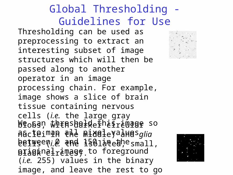
Thresholding can be used as preprocessing to extract an interesting subset of image structures which will then be passed along to another operator in an image processing chain. For example, image shows a slice of brain tissue containing nervous cells (i.e. the large gray blobs, with darker circular nuclei in the middle) and glia cells (i.e. the isolated, small, black circles).

We can threshold this image so as to map all pixel values between 0 and 150 in the original image to foreground (i.e. 255) values in the binary image, and leave the rest to go to background, as in

Global Thresholding - Guidelines for Use

If we wanted to know how many nerve cells there are in the original image, we might try applying a double threshold in order to select out just the pixels which correspond to nerve cells (and therefore have middle level grayscale intensities) in the original image. (In remote sensing and medical terminology, such thresholding is usually called density slicing.) Applying a threshold band of 130 - 150 yields

The resultant image can then be connected-components-labeled in order to count the total number of cells in the original image, as in

Thresholding in RGB space

For color or multi-spectral images, it may be possible to set different thresholds for each color channel, and so select just those pixels within a specified cuboid in RGB space. Another common variant is to set to black all those pixels corresponding to background, but leave foreground pixels at their original color/intensity (as opposed to forcing them to white), so that that information is not lost.

max

max

),(0

),(,1),(

dyxd

dyxdyxg

2

0

2

0

2

0 ),(),(),(),( ByxfGyxfRyxfyxd BGR

where

Adaptive Thresholding

A more complex thresholding algorithm would be to use a spatially varying threshold. This approach is very useful to compensate for the effects of non –uniform illumination. If T depends on coordinates x and y, this referred to as Dynamic Thresholding or Adaptive Thresholding.

Another approach is to perform a preprocessing step before thresholding.

Preprocessing the image to remove noise of other non-uniformities can improve the performance of the thresholding.

A technique which often provides better results is to only use edge points when creating the grey level histogram .

Adaptive thresholding - how it works?

There are two main approaches to finding the threshold:

(i) the Chow and Kaneko approach and

(ii) local thresholding.

The assumption behind both methods is that smaller image regions are more likely to have approximately uniform illumination, thus being more suitable for thresholding.

Chow and Kaneko divide an image into an array of overlapping subimages and then find the optimum threshold for each subimage by investigating its histogram. The threshold for each single pixel is found by interpolating the results of the subimages. The drawback of this method is that it is computational expensive and, therefore, is not appropriate for real-time applications.

An alternative approach to finding the local threshold is to statistically examine the intensity values of the local neighborhood of each pixel. The statistic which is most appropriate depends largely on the input image. Simple and fast functions include the mean of the local intensity distribution,

Adaptive thresholding - Local thresholding

the median value,

or the mean of the minimum and maximum values,

The size of the neighborhood has to be large enough to cover sufficient foreground and background pixels, otherwise a poor threshold is chosen. On the other hand, choosing regions which are too large can violate the assumption of approximately uniform illumination. This method is less computationally intensive than the Chow and Kaneko approach and produces good results for some applications.

Adaptive thresholding -Guidelines for Use Local adaptive thresholding, on the other hand, selects an individual threshold for each pixel based on the range of intensity values in its local neighborhood. This allows for thresholding of an image whose global intensity histogram doesn't contain distinctive peaks.

A task well suited to local adaptive thresholding is in segmenting text from the image

Because this image contains a strong illumination gradient, global thresholding produces a very poor result, as can be seen in

Adaptive thresholding -Guidelines for UseUsing the mean of a 7×7 neighborhood, adaptive thresholding yields

The method succeeds in the area surrounding the text because there are enough foreground and background pixels in the local neighborhood of each pixel; i.e. the mean value lies between the intensity values of foreground and background and, therefore, separates easily. On the margin, however, the mean of the local area is not suitable as a threshold, because the range of intensity values within a local neighborhood is very small and their mean is close to the value of the center pixel.

Adaptive thresholding -Guidelines for Use

The situation can be improved if the threshold employed is not the mean, but (mean-C), where C is a constant. Using this statistic, all pixels which exist in a uniform neighborhood (e.g. along the margins) are set to background. The result for a 7×7 neighborhood and C=7 is shown in

and for a 75×75 neighborhood and C=10 in

The larger window yields the poorer result, because it is more adversely affected by the illumination gradient. Also note that the latter is more computationally intensive than thresholding using the smaller window.

Adaptive thresholding -Guidelines for UseThe result of using the median instead of the mean can be seen in

The neighborhood size for this example is 7×7 and C = 4). The result shows that, in this application, the median is a less suitable statistic than the mean.

Adaptive thresholding -Guidelines for Use

Consider another example image containing a strong illumination gradient

This image can not be segmented with a global threshold, as shown in

where a threshold of 80 was used.

However, since the image contains a large object, it is hard to apply adaptive thresholding, as well. Using the (mean - C) as a local threshold, we obtain with a 7×7 window and C

= 4

Adaptive thresholding -Guidelines for Use

Using the (mean - C) as a local threshold, we obtain

with a 140×140 window and C = 8. All pixels which belong to the object but do not have any background pixels in their neighborhood are set to background. The latter image shows a much better result than that achieved with a global threshold, but it is still missing some pixels in the center of the object. In many applications, computing the mean of a neighborhood (for each pixel!) whose size is of the order 140×140 may take too much time. In this case, the more complex Chow and Kaneko approach to adaptive thresholding would be more successful.

Adaptive thresholding algorithm

You can simulate the effect with the following steps:

1. Convolve the image with a suitable statistical operator, i.e. the mean or median.

2. Subtract the original from the convolved image.

3. Threshold the difference image with C.

4. Invert the thresholded image.

Segmentation - Conclusions

• identify pixels that belong to features of interest

• first step in automatic image analysis and interpretation

• applications involving detection, recognition, or measurement of features

• non-contextual techniques

- ignore relationships between pixels of a feature

- group pixels based on a global attribute

• contextual

- exploit relationships between pixels of a feature (e.g. proximity)

Thresholding - Conclusions* non-contextual approach

*used for solid objects resting on a contrasting background

* may threshold on gray level

* generates a binary image

- assign 1 (or 255) to pixels with gray levels of interest

- assign 0 to the rest

* may have one or two thresholds

* may implement via a lookup table

* picking the threshold is the hard part

--human operator - GrayMapTool application

--preselected threshold

--mean gray level

--fixed percentage of pixels selected

--choose a point between two peaks in the histogram

Contextual techniques for image segmentation

• pixels belonging to the same object are close to each other

• we look at proximity as well as gray level

approaches based on discontinuity

•e.g. use edge detection to identify the boundary of a region

•can be difficult to generate a complete boundary (no holes)

approaches based on similarity

- group pixels together based on similarity and proximity

- specify similarity criteria