SEGREGATION IN CLASSROOMS USING

THE SCHELLING MODEL Olof Nilsson Camilla Öhman Project in Computational Science: Report February 2014

DEPARTMENT OF INFORMATION TECHNOLOGY

PR

OJE

CT

REP

OR

T

2

3

Abstract

The Schelling model is used to simulate classroom segregation. The simulations of the model show that segregated patterns occur even for weak preferences on neighbouring classmates. It shows that if unsatisfied individuals chose a new seating location according to the given algorithm, rather than randomly, equilibrium is reached just within a few iteration steps. Although, if the moving is random, the population’s overall satisfaction is higher than if the moving is according to the algorithm, if the individuals have preferences on many neighbours.

Based on initial hypotheses of the simulations, a real-time multiplayer game was developed for later experiments in upper secondary school classes. After analysing outcomes from the simulations, the parameters of the game were changed to better match the model. The game was pilot tested twice, and worked as intended. However, drawing conclusions from the model, when used with active choices by individuals, cannot be done due to lack of statistical significance.

4

5

CONTENTS

1 INTRODUCTION ................................................................................................................................ 6

1.1 BACKGROUND ................................................................................................................................................................ 6 1.2 THE SCHELLING MODEL ............................................................................................................................................. 6 1.3 AIM OF THIS PROJECT................................................................................................................................................... 6

2 METHOD .............................................................................................................................................. 7

2.1 MATLAB SIMULATION MODEL ................................................................................................................................. 7 2.2 IMPLEMENTING THE GAME ......................................................................................................................................... 9

2.2.1 Overview .......................................................................................................................................................... 9 2.2.2 Game logics and visualisations .............................................................................................................. 9 2.2.3 Multiplayer in real-time ..........................................................................................................................10 2.2.4 The website ...................................................................................................................................................11 2.2.5 Data storage ................................................................................................................................................12

2.3 JAVASCRIPT SIMULATION MODEL ........................................................................................................................... 13

3 RESULTS ............................................................................................................................................ 15

3.1 MATLAB SIMULATIONS .......................................................................................................................................... 15 3.1.1 Simulation of smart moving ..................................................................................................................16 3.1.2 Simulation of random moving ..............................................................................................................17 3.1.3 Simulation of both smart and random moving.............................................................................19 3.1.4 Simulation of smart moving – semi-happy if dissimilarity fulfilled .....................................22 3.1.5 Simulation of smart moving – finding fully happy first, semi-happy if dissimilarity or similarity fulfilled.........................................................................................................................................................22

3.2 RESULTS FROM THE GAME ....................................................................................................................................... 24

4 DISCUSSION ...................................................................................................................................... 27

4.1 SIMULATION ............................................................................................................................................................... 27 4.2 GAME ........................................................................................................................................................................... 28

ACKNOWLEDGEMENTS ........................................................................................................................... 28

REFERENCES .............................................................................................................................................. 29

6

1 Introduction

1.1 Background Segregation is today a widely debated subject, both scientifically as well as politically. It exists in many different aspects such as sex, age, income, language, religion, ethnicity and taste. In the two papers by T. C. Schelling [1][2], he states that some segregation results from the practices of organizations, some is deliberately organized and some results from the interplay of individual choices that discriminate. Some segregation directly correlates to other, e.g. how people choose to seat in a classroom depends on the selection of individuals attending the specific school, which in turn is highly dependent on its geographical positioning and the surrounding residential situation.

As shown by G. E. Birkelund and Y. Lemel [3], social gaps and inequalities in educational performance may be a direct consequence from segregation. In order to prevent segregation it is of high importance to understand why and how it occurs. The Schelling model, first proposed by the American economist Thomas C. Schelling in 1969 [1][2], implies that segregation is inevitable in some situations even where individuals do not have preference for segregation. Equilibrium states in a twofold defined population may consist of clusters of only one sort of individual although they all share a preference to include the opposite group.

1.2 The Schelling Model The population consists of two types. Each type has a number of agents, which are (randomly) placed in a grid with fixed boundaries. If the population is an uneven number, one of the population types will have one more agent than the other. The agents are considered to have a Moore neighbourhood, i.e. the eight closest spots to an agent are included in its neighbourhood. If an agent is placed next to any of the sides, the neighbourhood includes only the spots within the grid (and the neighbourhood is less than eight spots). If an agent is unhappy with its current neighbourhood composition, it will move to a neighbourhood where it will be happier, if such exists.

In the simulations, the agent will move to the closest spot where the agent’s demands are fulfilled. This moving rule is later on in this report referred to as smart moving. When all agents are satisfied with their spot, or when no agent can move to a spot where it would be happier, the simulation (or the game) stops. The demands that an agent has on its neighbourhood are in number of certain neighbour types, and not in percentage of certain neighbour types.

1.3 Aim of this project This report focuses on segregation related to seating in classrooms. The project was a part of a bigger project at the Institute for Future Studies (IFFS) in Stockholm, a project with a twofold goal: to demonstrate basic concepts of

7

segregation to students according to the Schelling model and to collect data on individual and collective behaviour for research, e.g. J.M. Benito et al. [4] and G. Ruoff and G. Schneider [5]. The data would then be used to test the following hypotheses:

H1 (Seating Observation). Segregation occurs naturally even along trivial

attributes.

H2 (Schelling Game). Segregation emerges in the absence of individual

incentives to segregate.

H3 (Integration Game). Segregation emerges even in the presence of

individual incentives to integrate.

The games that the hypotheses refer to were desired to be played on game “consoles” for each student, but to have the actual game projected on a screen. After students have played the game, they would work with a mathematical model simulation of what they did in the game.

The project, described in this report, consisted of developing the game with data storage as well as creating the model simulation and exploring how different settings in the model would affect the outcomes. First, we use MATLAB to simulate how the game rules and other settings affect the game outcomes and to see how robust the model is with respect to some of the assumptions. This is done by varying the demands on type of neighbours, as well as the population size and the moving rule. These results are later used when implementing the settings in the game.

A JavaScript simulation is used for visual demonstration of the Schelling model. Students will, after the game experiment, explore the model and be able to compare simulation results from a mathematical model with the results from the game. The site consists of a grid where the simulation is visualised, option settings and (after performed simulation) two graphs with results. The idea is that students will try different settings for the model (grid size, population size, preferences on neighbours) and see what outcomes they yield.

The game will interactively demonstrate to the students, how their active choices (following some predetermined rule) may cause segregated patterns to arise. It will also be used to collect data on where students choose to sit in relation to their classmates.

2 Method

2.1 MATLAB simulation model In the MATLAB simulation, the impact of the population size on the resulting total number of happy agents was investigated for different settings called Case 1-Case 13; see explanation in Table 1. The impact is then considered when choosing which population size to use in the graphs of how the overall similarity

8

depends on the individual preferences. Case 0-Case 6 and Case 8-16 are used in simulations for these certain population sizes.

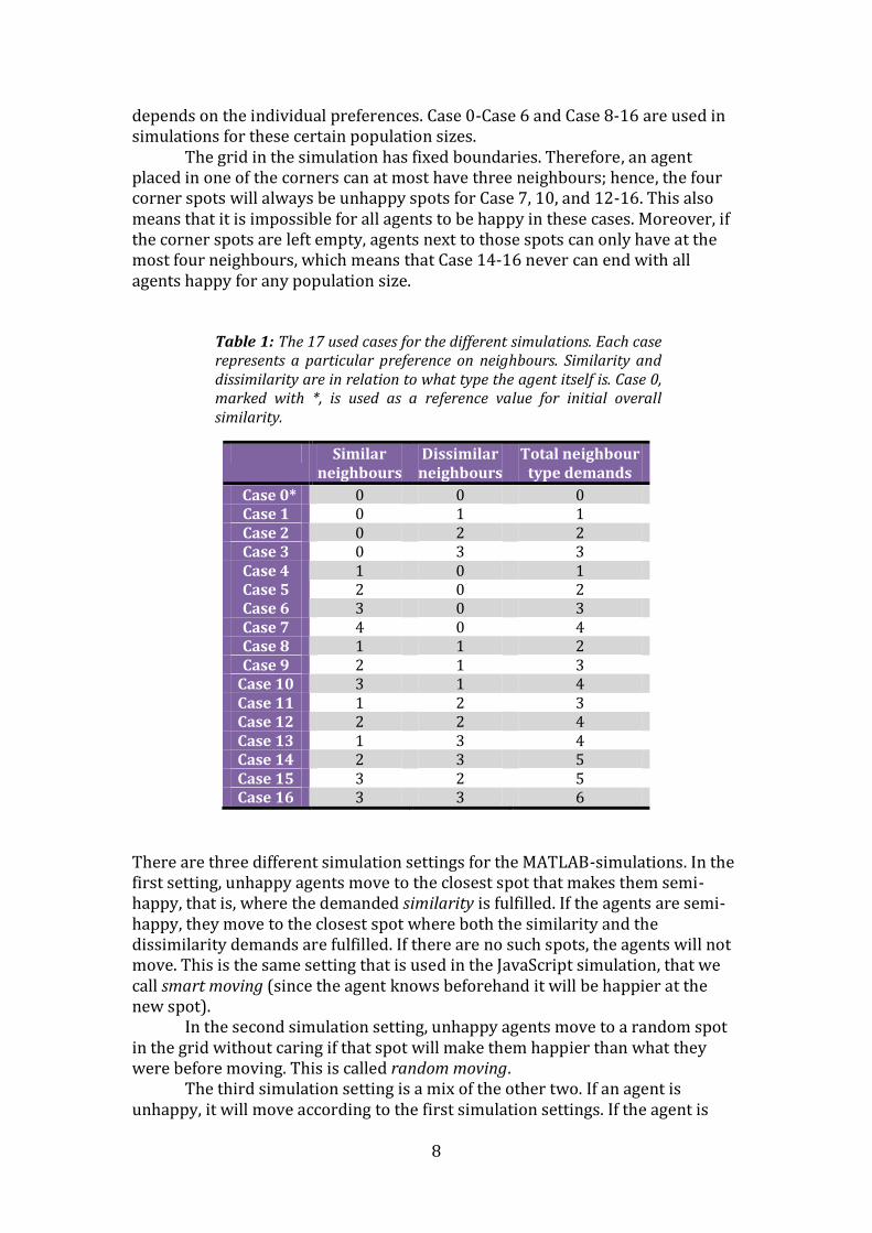
The grid in the simulation has fixed boundaries. Therefore, an agent placed in one of the corners can at most have three neighbours; hence, the four corner spots will always be unhappy spots for Case 7, 10, and 12-16. This also means that it is impossible for all agents to be happy in these cases. Moreover, if the corner spots are left empty, agents next to those spots can only have at the most four neighbours, which means that Case 14-16 never can end with all agents happy for any population size.

Table 1: The 17 used cases for the different simulations. Each case represents a particular preference on neighbours. Similarity and dissimilarity are in relation to what type the agent itself is. Case 0, marked with *, is used as a reference value for initial overall similarity.

Similar neighbours

Dissimilar neighbours

Total neighbour type demands

Case 0* 0 0 0 Case 1 0 1 1 Case 2 0 2 2 Case 3 0 3 3 Case 4 1 0 1 Case 5 2 0 2 Case 6 3 0 3 Case 7 4 0 4 Case 8 1 1 2 Case 9 2 1 3

Case 10 3 1 4 Case 11 1 2 3 Case 12 2 2 4 Case 13 1 3 4 Case 14 2 3 5 Case 15 3 2 5 Case 16 3 3 6

There are three different simulation settings for the MATLAB-simulations. In the first setting, unhappy agents move to the closest spot that makes them semi-happy, that is, where the demanded similarity is fulfilled. If the agents are semi-happy, they move to the closest spot where both the similarity and the dissimilarity demands are fulfilled. If there are no such spots, the agents will not move. This is the same setting that is used in the JavaScript simulation, that we call smart moving (since the agent knows beforehand it will be happier at the new spot).

In the second simulation setting, unhappy agents move to a random spot in the grid without caring if that spot will make them happier than what they were before moving. This is called random moving.

The third simulation setting is a mix of the other two. If an agent is unhappy, it will move according to the first simulation settings. If the agent is

9

unable to move to a spot that will make it happier, it will move random, as in the second simulation.

Moreover, the semi-happy condition’s impact on the resulting similarity was investigated by testing what happens if instead semi-happy would be defined as having the demanded dissimilarity fulfilled, as well as changing the moving rule so that agents would always primarily search for a spot where both demands are fulfilled, and secondarily for a spot where just the semi-happy condition is fulfilled.

2.2 Implementing the game

2.2.1 Overview

There exist numerous different approaches to implement a real-time online multiplayer game. The most common one today for this type of games is perhaps applications developed for mobile operating systems (OS). The downside with this is that one application alone cannot be used to run on each of the mobile specific OSs. Considering this and taking into account the timeframe of the project, it was decided to program a web-based version accessible from as many platforms as possible. Deciding to go with a web-based game does however introduce several surrounding factors to the actual game play, e.g. the game is not reachable by a single click on an application but rather each player of the game needs to actively connect to it through a web request. This requires programming using different languages, frameworks and extensions. In the list below an outline of each of the programming needed steps is written.

Routing and structuring the website, including cookie handling Server and client connections, including real-time

requests/commands Game logics and visualisations Storing and handling data

Except for parts of the first point and, in some sense, the visualisation, everything is programmed in JavaScript, with different frameworks and extensions to handle the different specific tasks. Each of the steps will be elaborated on in the subsections following.

2.2.2 Game logics and visualisations

The first implemented part was the game logics, written using plain JavaScript. Starting off, a single player offline version was designed and thoroughly bug tested to reduce unnecessary obstacles later on. A player is able to move in a squared grid and moves either up, down, left or right but not exceeding the borders in any direction. A coloured circle containing a unique ID represents each player (later on referred to as avatar). This is visualised using HTML5

10

canvas, a convenient tool for dynamic rendering of 2D shapes and bitmap images in a web browser.

2.2.3 Multiplayer in real-time

Recent experiments on classroom segregation have been made, e.g. Ruoff and Schneider [5]. To our knowledge, there exist no such experiment where movement decisions happen in real-time rather than in turns (discrete time). To have multiple clients simultaneously playing the same game with one client’s decision possibly affecting other clients, communication needs to flow between them in some way. This can either be achieved by direct communication amongst all connected clients (i.e. peer to peer) or by using a server as a communication hub. In the latter, data are sent from each client to the server, which in turn processes the received data and then, possibly, broadcasts the resulting data to the affected clients.

There are two main reasons why this communication flow suited this game better and therefore was chosen. Firstly, not all data are required to be transmitted amongst clients. Secondly, and perhaps most vitally, this allows for all game logics to be handled at a single location making synchronisations far more easily handled as well as efficient. If any given control check was to be made on the client side, all other clients would have to be locked in the meantime to prevent conflicts, such as two players moving to the very same spot. This particular example could occur when the game logic is located on the client side, if the two players decide to move to the same spot at roughly the same time with inevitable lag in communication making one of the players unaware that the spot is actually already occupied. It was decided to program the connections and communication using WebSockets, a recently developed protocol providing full-duplex communication meaning that data are allowed to stream simultaneously in both directions. Despite WebSockets being a novel addition to HTML, it already by now is compatible with the vast majority of commercial web browsers (Can I use [6]), which was the most important argument to its use.

The particular application programming interface (API) used is called Socket.io [7], consisting of two similar JavaScript libraries; one for the server side running on Node.js and one for the client side running in a supporting web browser. Node.js [8] is a software platform also utilising JavaScript, designed for scalable network applications. A common way to go about programming applications today is to find an open source project with code structures applicable for your use. To add the multiplayer functionality in the game, the code of Rob Hawke’s tutorial [9] on multiplayer games developed with WebSockets was used as a skeleton. The structure was heavily revised and built upon to match the single player version as well as the surrounding code not directly belonging to the gameplay.

With the multiplayer implementation in place, every player is now able to move up, down, left or right to the next spot not occupied by another player if such a spot momentarily exists. The starting position of each player is randomly

11

distributed. Every second connecting player is given the same colour, making it in some sense random as well since no player will know exactly when another player will join. A game will continue until all players are satisfied with their current location (according to the prescribed rule) or at most three minutes.

2.2.4 The website

Programming wise, there are a lot of procedures both prior to and post the game taking place. The server has to distinguish each individual in a smart way to later on store data in an unambiguous manner. Also, it needs to route visitors correctly depending on what they have or have not already done. For instance, if an individual who has already entered the game, gets disconnected, the server needs to recognise this and redirect the revisiting individual to the game and reconnect him or her to his/her last position when the connection was disrupted.

Express.js [10] is a web application framework for Node.js providing this functionality by handling basic HTTP requests (such as GET and POST), as well as setting up and managing cookies and sessions.

It was necessary to divide the website into two separate interfaces: one for the experimenter (later on referred to as admin) and one for the subjects of the experiment (later on referred to as players). Prior to the game, the admin will be routed to a configuration page to set up the game matching the properties of the visited classroom, whereas the players will instead be routed to a survey where their answers will be saved and later on displayed to them. The questions in the survey and the answer options was phrased as follows:

What is your gender? Male/Female Which pet do you prefer? Cat/Dog Which subject do you like more? Literature/Math In your free time, where would you rather be? In front of a

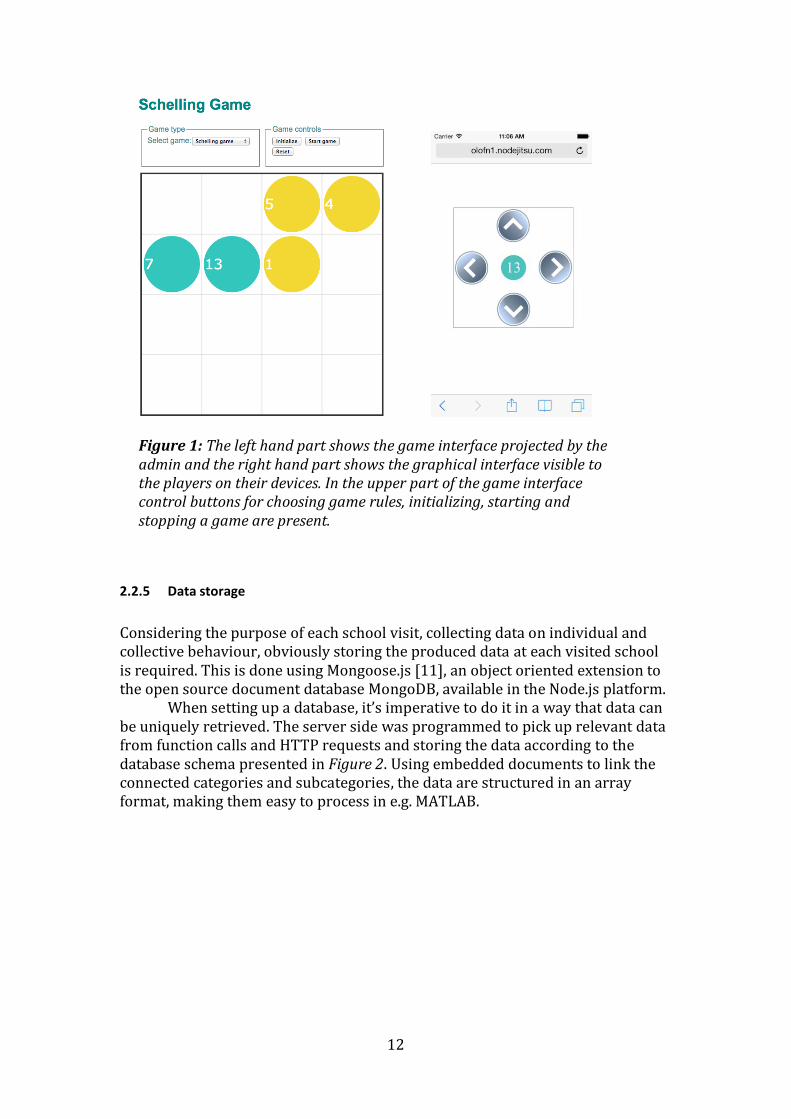
computer/Outdoors with friends When playing the game, the players will only see their own avatar and the control buttons on their own device. The admin will project the game on a screen for everyone to see. The visual interfaces are shown in Figure 1. Who is being routed to where on the page is determined through a login page in the very first step, where each player enters their unique ID handed to them depending on where in the classroom they are seated. The admin instead enters a predetermined login ID. Using the Express library, each client is then assigned a local cookie depending on their ID and a matching session is stored on the server side for recognition throughout the experiment.

12

Figure 1: The left hand part shows the game interface projected by the admin and the right hand part shows the graphical interface visible to the players on their devices. In the upper part of the game interface control buttons for choosing game rules, initializing, starting and stopping a game are present.

2.2.5 Data storage

Considering the purpose of each school visit, collecting data on individual and collective behaviour, obviously storing the produced data at each visited school is required. This is done using Mongoose.js [11], an object oriented extension to the open source document database MongoDB, available in the Node.js platform.

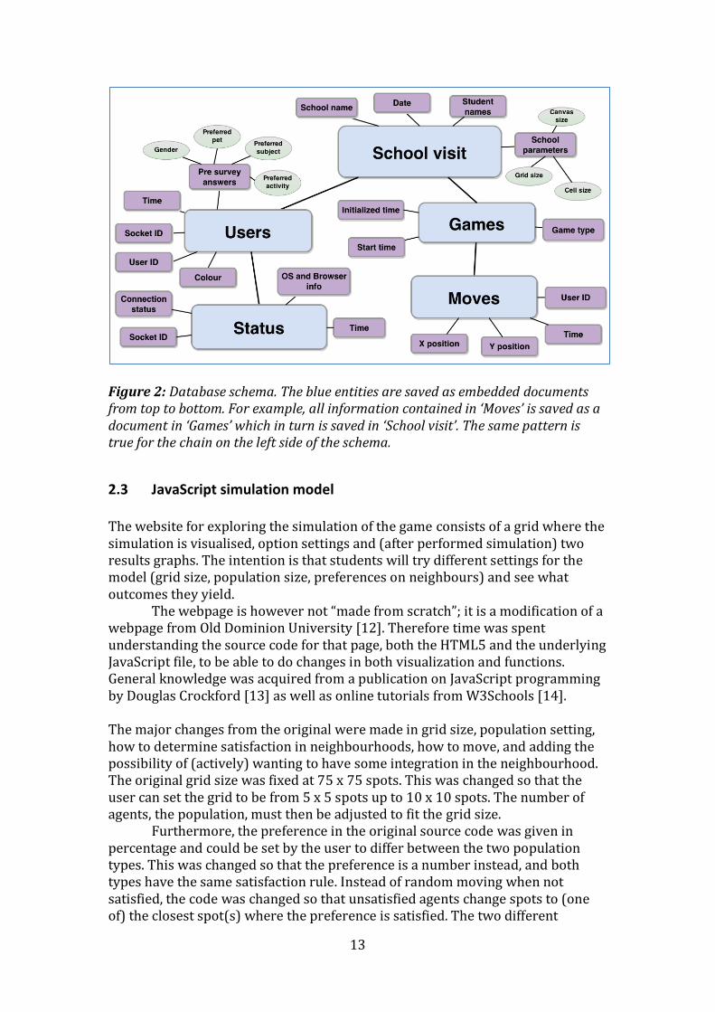
When setting up a database, it’s imperative to do it in a way that data can be uniquely retrieved. The server side was programmed to pick up relevant data from function calls and HTTP requests and storing the data according to the database schema presented in Figure 2. Using embedded documents to link the connected categories and subcategories, the data are structured in an array format, making them easy to process in e.g. MATLAB.

13

Figure 2: Database schema. The blue entities are saved as embedded documents from top to bottom. For example, all information contained in ‘Moves’ is saved as a document in ‘Games’ which in turn is saved in ‘School visit’. The same pattern is true for the chain on the left side of the schema.

2.3 JavaScript simulation model The website for exploring the simulation of the game consists of a grid where the simulation is visualised, option settings and (after performed simulation) two results graphs. The intention is that students will try different settings for the model (grid size, population size, preferences on neighbours) and see what outcomes they yield.

The webpage is however not “made from scratch”; it is a modification of a webpage from Old Dominion University [12]. Therefore time was spent understanding the source code for that page, both the HTML5 and the underlying JavaScript file, to be able to do changes in both visualization and functions. General knowledge was acquired from a publication on JavaScript programming by Douglas Crockford [13] as well as online tutorials from W3Schools [14]. The major changes from the original were made in grid size, population setting, how to determine satisfaction in neighbourhoods, how to move, and adding the possibility of (actively) wanting to have some integration in the neighbourhood. The original grid size was fixed at 75 x 75 spots. This was changed so that the user can set the grid to be from 5 x 5 spots up to 10 x 10 spots. The number of agents, the population, must then be adjusted to fit the grid size.

Furthermore, the preference in the original source code was given in percentage and could be set by the user to differ between the two population types. This was changed so that the preference is a number instead, and both types have the same satisfaction rule. Instead of random moving when not satisfied, the code was changed so that unsatisfied agents change spots to (one of) the closest spot(s) where the preference is satisfied. The two different

14

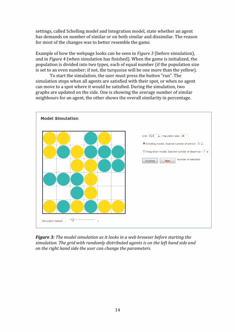
settings, called Schelling model and Integration model, state whether an agent has demands on number of similar or on both similar and dissimilar. The reason for most of the changes was to better resemble the game. Example of how the webpage looks can be seen in Figure 3 (before simulation), and in Figure 4 (when simulation has finished). When the game is initialized, the population is divided into two types, each of equal number (if the population size is set to an even number; if not, the turquoise will be one more than the yellow).

To start the simulation, the user must press the button “run”. The simulation stops when all agents are satisfied with their spot, or when no agent can move to a spot where it would be satisfied. During the simulation, two graphs are updated on the side. One is showing the average number of similar neighbours for an agent, the other shows the overall similarity in percentage.

Figure 3: The model simulation as it looks in a web browser before starting the simulation. The grid with randomly distributed agents is on the left hand side and on the right hand side the user can change the parameters.

15

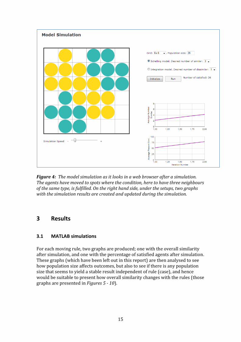
Figure 4: The model simulation as it looks in a web browser after a simulation. The agents have moved to spots where the condition, here to have three neighbours of the same type, is fulfilled. On the right hand side, under the setups, two graphs with the simulation results are created and updated during the simulation.

3 Results

3.1 MATLAB simulations For each moving rule, two graphs are produced; one with the overall similarity after simulation, and one with the percentage of satisfied agents after simulation. These graphs (which have been left out in this report) are then analysed to see how population size affects outcomes, but also to see if there is any population size that seems to yield a stable result independent of rule (case), and hence would be suitable to present how overall similarity changes with the rules (those graphs are presented in Figures 5 - 10).

16

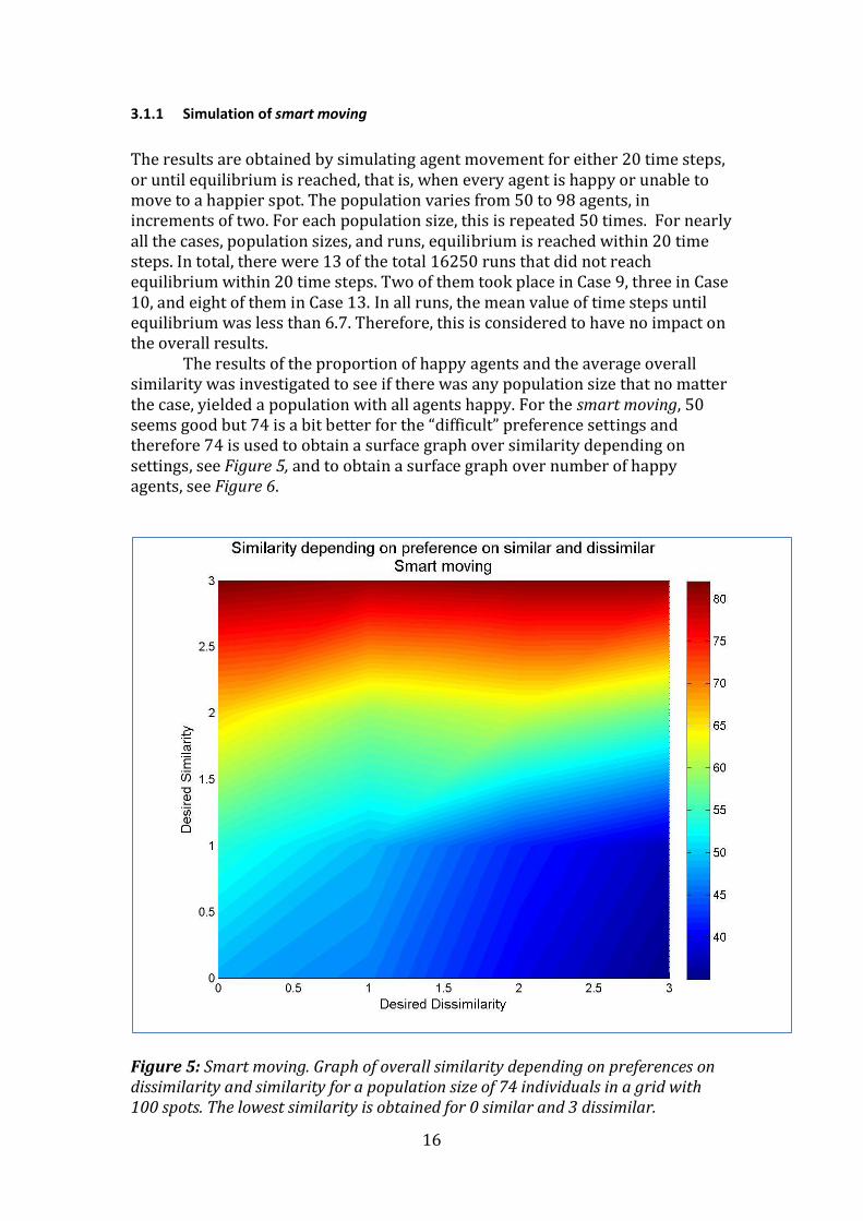
3.1.1 Simulation of smart moving

The results are obtained by simulating agent movement for either 20 time steps, or until equilibrium is reached, that is, when every agent is happy or unable to move to a happier spot. The population varies from 50 to 98 agents, in increments of two. For each population size, this is repeated 50 times. For nearly all the cases, population sizes, and runs, equilibrium is reached within 20 time steps. In total, there were 13 of the total 16250 runs that did not reach equilibrium within 20 time steps. Two of them took place in Case 9, three in Case 10, and eight of them in Case 13. In all runs, the mean value of time steps until equilibrium was less than 6.7. Therefore, this is considered to have no impact on the overall results.

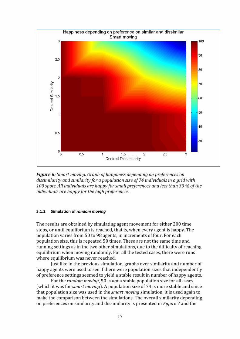
The results of the proportion of happy agents and the average overall similarity was investigated to see if there was any population size that no matter the case, yielded a population with all agents happy. For the smart moving, 50 seems good but 74 is a bit better for the “difficult” preference settings and therefore 74 is used to obtain a surface graph over similarity depending on settings, see Figure 5, and to obtain a surface graph over number of happy agents, see Figure 6.

Figure 5: Smart moving. Graph of overall similarity depending on preferences on dissimilarity and similarity for a population size of 74 individuals in a grid with 100 spots. The lowest similarity is obtained for 0 similar and 3 dissimilar.

17

Figure 6: Smart moving. Graph of happiness depending on preferences on dissimilarity and similarity for a population size of 74 individuals in a grid with 100 spots. All individuals are happy for small preferences and less than 30 % of the individuals are happy for the high preferences.

3.1.2 Simulation of random moving

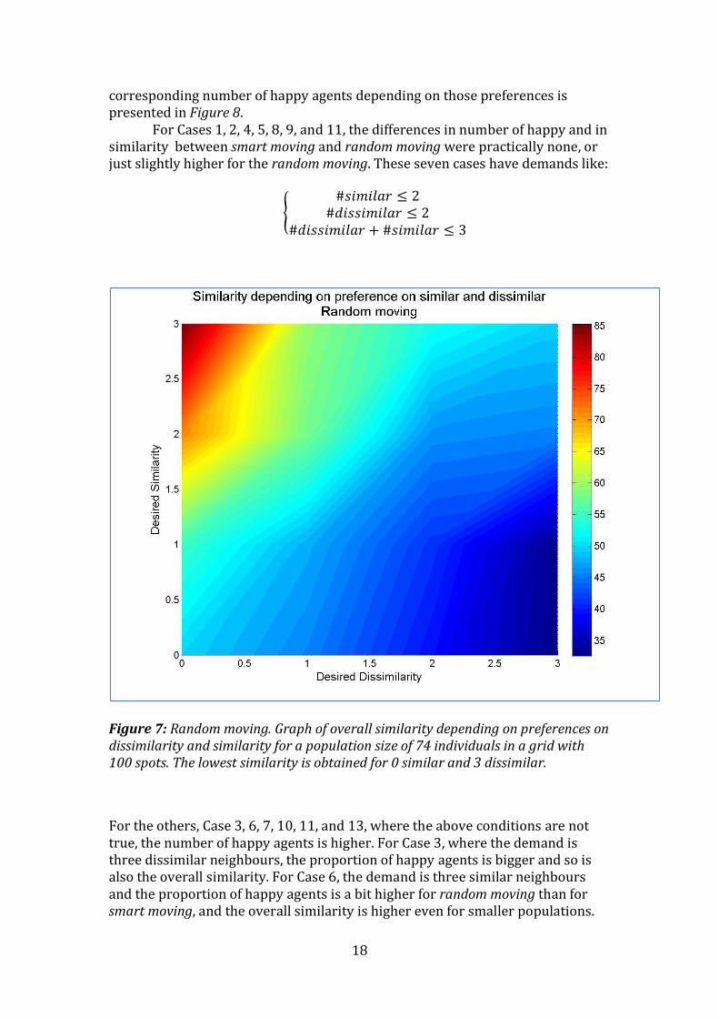
The results are obtained by simulating agent movement for either 200 time steps, or until equilibrium is reached, that is, when every agent is happy. The population varies from 50 to 98 agents, in increments of four. For each population size, this is repeated 50 times. These are not the same time and running settings as in the two other simulations, due to the difficulty of reaching equilibrium when moving randomly. For all the tested cases, there were runs where equilibrium was never reached.

Just like in the previous simulation, graphs over similarity and number of happy agents were used to see if there were population sizes that independently of preference settings seemed to yield a stable result in number of happy agents.

For the random moving, 50 is not a stable population size for all cases (which it was for smart moving). A population size of 74 is more stable and since that population size was used in the smart moving simulation, it is used again to make the comparison between the simulations. The overall similarity depending on preferences on similarity and dissimilarity is presented in Figure 7 and the

18

corresponding number of happy agents depending on those preferences is presented in Figure 8.

For Cases 1, 2, 4, 5, 8, 9, and 11, the differences in number of happy and in similarity between smart moving and random moving were practically none, or just slightly higher for the random moving. These seven cases have demands like:

Figure 7: Random moving. Graph of overall similarity depending on preferences on dissimilarity and similarity for a population size of 74 individuals in a grid with 100 spots. The lowest similarity is obtained for 0 similar and 3 dissimilar.

For the others, Case 3, 6, 7, 10, 11, and 13, where the above conditions are not true, the number of happy agents is higher. For Case 3, where the demand is three dissimilar neighbours, the proportion of happy agents is bigger and so is also the overall similarity. For Case 6, the demand is three similar neighbours and the proportion of happy agents is a bit higher for random moving than for smart moving, and the overall similarity is higher even for smaller populations.

19

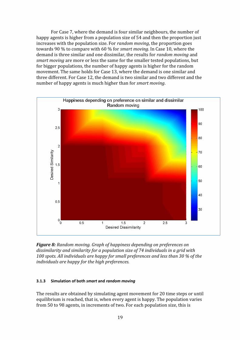
For Case 7, where the demand is four similar neighbours, the number of happy agents is higher from a population size of 54 and then the proportion just increases with the population size. For random moving, the proportion goes towards 90 % to compare with 60 % for smart moving. In Case 10, where the demand is three similar and one dissimilar, the results for random moving and smart moving are more or less the same for the smaller tested populations, but for bigger populations, the number of happy agents is higher for the random movement. The same holds for Case 13, where the demand is one similar and three different. For Case 12, the demand is two similar and two different and the number of happy agents is much higher than for smart moving.

Figure 8: Random moving. Graph of happiness depending on preferences on dissimilarity and similarity for a population size of 74 individuals in a grid with 100 spots. All individuals are happy for small preferences and less than 30 % of the individuals are happy for the high preferences.

3.1.3 Simulation of both smart and random moving

The results are obtained by simulating agent movement for 20 time steps or until equilibrium is reached, that is, when every agent is happy. The population varies from 50 to 98 agents, in increments of two. For each population size, this is

20

repeated 50 times. All runs for Case 1, 2, and 3 and population sizes reached equilibrium within 20 time steps. For the other cases, there were runs that ended without reaching equilibrium.

The differences between simulations for smart moving, and smart and random moving are smaller than between smart moving and random moving. Case 1-5, Case 8-9, and Case 11-13 have nearly the same outcomes in the two simulations. Case 6 has the same proportion of number of happy agents, but a slightly higher overall similarity for smart and random moving. For Case 7, the proportion of happy agents is very varied in both simulation types, but, in the simulation with smart moving, the variation is between 20 % and 100 % for the smaller populations and 40 % and 70 % for larger populations, and in the simulation with smart and random moving, the variation is between 80 % and 100 %. The overall similarity is more consistent (between 80 % and 100 %) than in the simulation with just smart moving. For Case 10, the results are pretty much the same but the overall similarity is a bit less varied.

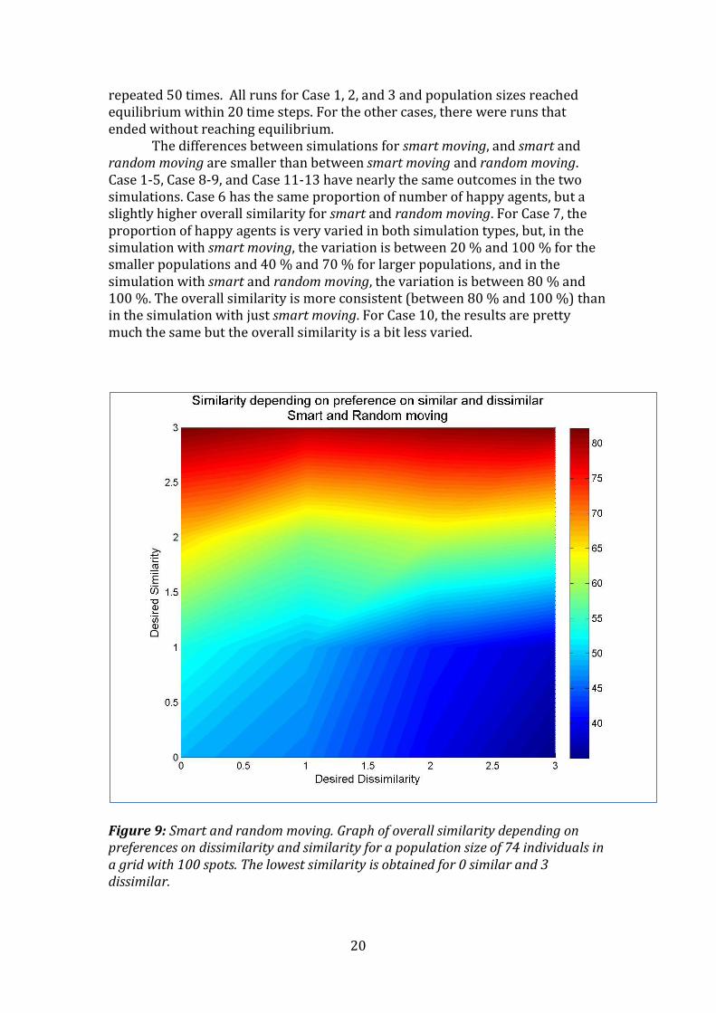
Figure 9: Smart and random moving. Graph of overall similarity depending on preferences on dissimilarity and similarity for a population size of 74 individuals in a grid with 100 spots. The lowest similarity is obtained for 0 similar and 3 dissimilar.

21

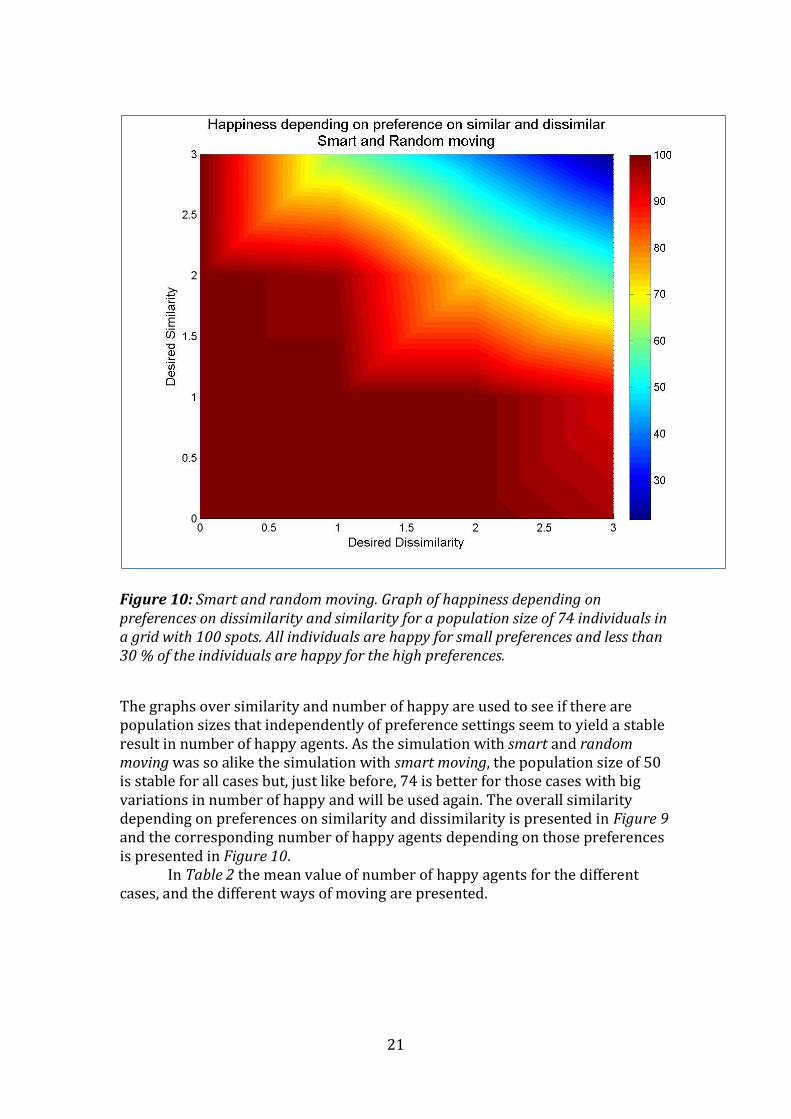
Figure 10: Smart and random moving. Graph of happiness depending on preferences on dissimilarity and similarity for a population size of 74 individuals in a grid with 100 spots. All individuals are happy for small preferences and less than 30 % of the individuals are happy for the high preferences.

The graphs over similarity and number of happy are used to see if there are population sizes that independently of preference settings seem to yield a stable result in number of happy agents. As the simulation with smart and random moving was so alike the simulation with smart moving, the population size of 50 is stable for all cases but, just like before, 74 is better for those cases with big variations in number of happy and will be used again. The overall similarity depending on preferences on similarity and dissimilarity is presented in Figure 9 and the corresponding number of happy agents depending on those preferences is presented in Figure 10. In Table 2 the mean value of number of happy agents for the different cases, and the different ways of moving are presented.

22

3.1.4 Simulation of smart moving – semi-happy if dissimilarity fulfilled

To see that the moving rules do not affect the results in an unwanted way and to see what would happen when agents have an incentive to first integrate, we simulated the overall similarity and the number of happy agents if the semi-happy condition instead was fulfilled when enough neighbours are dissimilar.

The results are practically identical for Case 1-6, which is expected since those cases only have demands on one type. For Case 8, where the demand is to have at least one similar and at least one dissimilar, the results for the proportion of happy agents and the overall similarity are the same (that is, all agents happy for populations smaller than 86 agents and almost always all agents happy for populations bigger than that, and an overall similarity around 50 %).

For Case 9, where the demand is at least two similar and at least one dissimilar, there are differences when taking care of the dissimilarity condition first. The variations in number of happy agents are less and for bigger populations, the proportions of happy agents are bigger. For the smaller populations the result is the same independent of which condition is fulfilled first. For the overall similarity, the variation is less and around 50 % instead of around 60 % as in the original moving condition.

For Case 10 the average proportion of happy agents varies around 80 % instead of the earlier 60 %. Although the setting for Case 10 is to have three similar and one dissimilar, no population size tested ends with all agents satisfied. The overall similarity is lower, around 60 % instead of 80 %. For bigger populations, the variation in similarity is less.

For Case 11 and Case 13 the results are the same as for taking care of the similarity condition first.

For Case 12, where the demand is to have two neighbours of each type, the variation in proportion of happy agents is less than in the settings where the similarity condition had to be fulfilled first: around 85 % instead of around 70 %. The overall similarity is also less varied, now around 40 % instead of 65 %.

3.1.5 Simulation of smart moving – finding fully happy first, semi-happy if dissimilarity

or similarity fulfilled

It is also simulated how the population happiness and similarity would evolve if the agents search primarily for a spot where both dissimilarity and similarity is fulfilled, and secondarily for spots where at least one of these preferences is fulfilled. Just as in the comparisons made with the dissimilarity-first condition, Cases 1-6 are identical due to the no demand on one of the types. For Case 8 this is also true. For Case 9, the proportion of happy agents is just slightly bigger than for the setting while finding spots where the similarity condition is fulfilled first. The overall similarity is slightly less.

Case 10 yields a big difference between the similarity-first settings and the both-conditions-first settings. The proportion of happy agents is overall bigger, and the variation for bigger populations is less. The overall similarity on

23

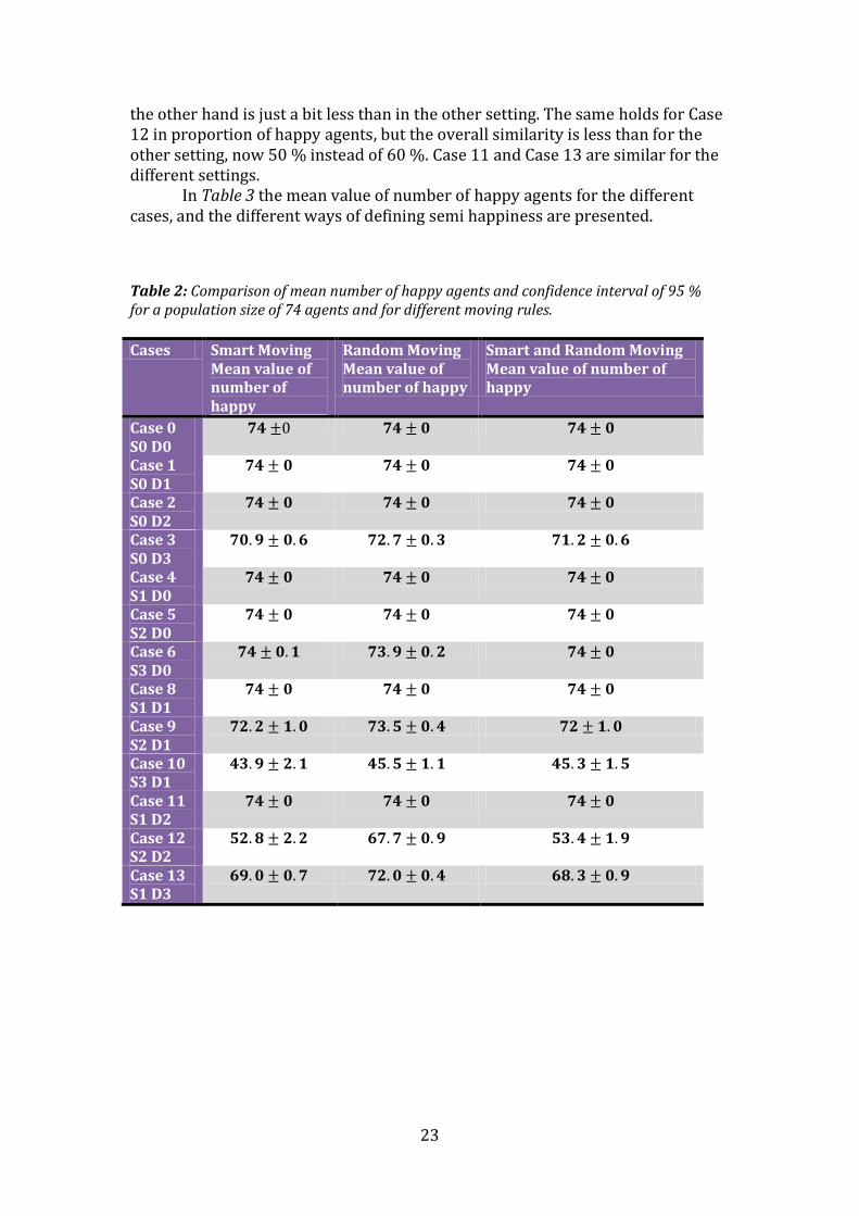
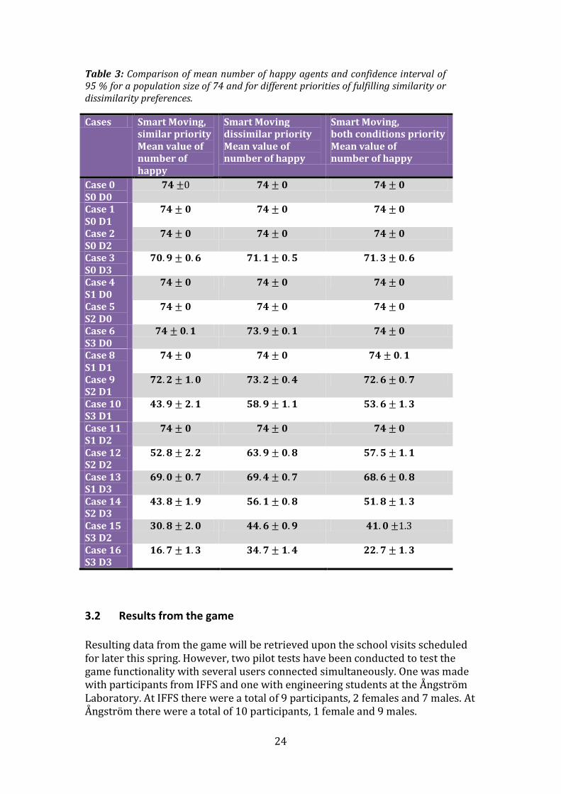
the other hand is just a bit less than in the other setting. The same holds for Case 12 in proportion of happy agents, but the overall similarity is less than for the other setting, now 50 % instead of 60 %. Case 11 and Case 13 are similar for the different settings. In Table 3 the mean value of number of happy agents for the different cases, and the different ways of defining semi happiness are presented. Table 2: Comparison of mean number of happy agents and confidence interval of 95 % for a population size of 74 agents and for different moving rules.

Cases Smart Moving Mean value of number of happy

Random Moving Mean value of number of happy

Smart and Random Moving Mean value of number of happy

Case 0 S0 D0

0

Case 1 S0 D1

Case 2 S0 D2

Case 3 S0 D3

Case 4 S1 D0

Case 5 S2 D0

Case 6 S3 D0

Case 8 S1 D1

Case 9 S2 D1

Case 10 S3 D1

Case 11 S1 D2

Case 12 S2 D2

Case 13 S1 D3

24

Table 3: Comparison of mean number of happy agents and confidence interval of 95 % for a population size of 74 and for different priorities of fulfilling similarity or dissimilarity preferences.

Cases Smart Moving, similar priority Mean value of number of happy

Smart Moving dissimilar priority Mean value of number of happy

Smart Moving, both conditions priority Mean value of number of happy

Case 0 S0 D0

0

Case 1 S0 D1

Case 2 S0 D2

Case 3 S0 D3

Case 4 S1 D0

Case 5 S2 D0

Case 6 S3 D0

Case 8 S1 D1

Case 9 S2 D1

Case 10 S3 D1

Case 11 S1 D2

Case 12 S2 D2

Case 13 S1 D3

Case 14 S2 D3

Case 15 S3 D2

1.3

Case 16 S3 D3

3.2 Results from the game Resulting data from the game will be retrieved upon the school visits scheduled for later this spring. However, two pilot tests have been conducted to test the game functionality with several users connected simultaneously. One was made with participants from IFFS and one with engineering students at the Ångström Laboratory. At IFFS there were a total of 9 participants, 2 females and 7 males. At Ångström there were a total of 10 participants, 1 female and 9 males.

25

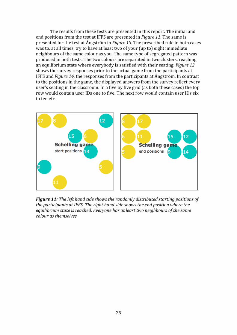
The results from these tests are presented in this report. The initial and end positions from the test at IFFS are presented in Figure 11. The same is presented for the test at Ångström in Figure 13. The prescribed rule in both cases was to, at all times, try to have at least two of your (up to) eight immediate neighbours of the same colour as you. The same type of segregated pattern was produced in both tests. The two colours are separated in two clusters, reaching an equilibrium state where everybody is satisfied with their seating. Figure 12 shows the survey responses prior to the actual game from the participants at IFFS and Figure 14, the responses from the participants at Ångström. In contrast to the positions in the game, the displayed answers from the survey reflect every user’s seating in the classroom. In a five by five grid (as both these cases) the top row would contain user IDs one to five. The next row would contain user IDs six to ten etc.

Figure 11: The left hand side shows the randomly distributed starting positions of the participants at IFFS. The right hand side shows the end position where the equilibrium state is reached. Everyone has at least two neighbours of the same colour as themselves.

26

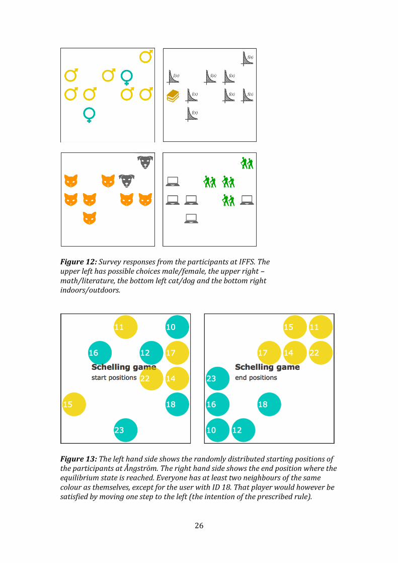
Figure 12: Survey responses from the participants at IFFS. The upper left has possible choices male/female, the upper right – math/literature, the bottom left cat/dog and the bottom right indoors/outdoors.

Figure 13: The left hand side shows the randomly distributed starting positions of the participants at Ångström. The right hand side shows the end position where the equilibrium state is reached. Everyone has at least two neighbours of the same colour as themselves, except for the user with ID 18. That player would however be satisfied by moving one step to the left (the intention of the prescribed rule).

27

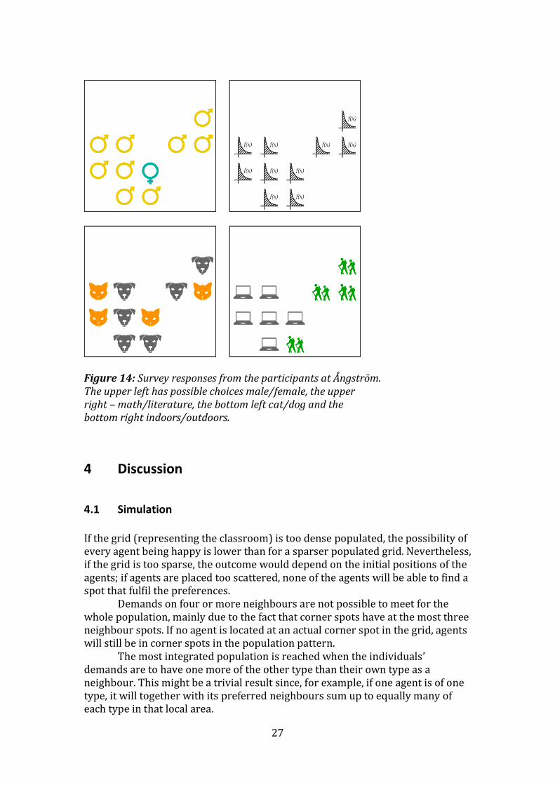
Figure 14: Survey responses from the participants at Ångström. The upper left has possible choices male/female, the upper right – math/literature, the bottom left cat/dog and the bottom right indoors/outdoors.

4 Discussion

4.1 Simulation If the grid (representing the classroom) is too dense populated, the possibility of every agent being happy is lower than for a sparser populated grid. Nevertheless, if the grid is too sparse, the outcome would depend on the initial positions of the agents; if agents are placed too scattered, none of the agents will be able to find a spot that fulfil the preferences.

Demands on four or more neighbours are not possible to meet for the whole population, mainly due to the fact that corner spots have at the most three neighbour spots. If no agent is located at an actual corner spot in the grid, agents will still be in corner spots in the population pattern.

The most integrated population is reached when the individuals’ demands are to have one more of the other type than their own type as a neighbour. This might be a trivial result since, for example, if one agent is of one type, it will together with its preferred neighbours sum up to equally many of each type in that local area.

28

Random moving yields more happy agents for the harder accomplished cases than smart moving, or smart and random moving. But one must keep in mind that the random moving simulations had more iteration steps in time than smart moving (10 times more) and hence the probability to fulfil satisfaction for agents increase. The smart moving is, in some sense, a very egocentric process since an agent’s movement can preclude others from being able to find any happy spot at all. The random moving is more solidarity. Also, random moving yields a more integrated population than smart moving.

4.2 Game The game is working as it was intended. With the experiments scheduled for later this spring, we have no statistical basis to draw conclusions from the results, as only two test runs have been performed so far.

However, comparing the outcome of the tests, it can be noted that the formulated hypotheses are indeed a possible outcome. Due to selection bias on gender and educational background in both tests, the survey responses lack variation. This will be important to take into account when deciding the orientation of the upper secondary schools to be visited. In both tests the only question with answers divided equally (approximately) was ‘In your free time, where would you rather be?’. From Figure 12 and Figure 14 it can be seen that the seating of the two groups are segregated in both cases. Again, with the lack of statistical significance this may very well merely be a coincidence.

Acknowledgements We would like to express our gratitude to our supervisors David J.T. Sumpter and Milena Tsvetkova, for assigning us this project and for their support along the project. We would also like to thank Cédric Morin, Henrik Boström and Yann Chazallon, students from the Royal Institute of Technology in Stockholm for their inputs on how to structure the multiplayer parts of the game.

29

References

[1] Schelling T.C. (1969). Models of Segregation. The American Economic Review, Vol. 59, No. 2, 488-493

[2] Schelling T.C. (1971). Dynamic Models of Segregation. The Journal of Mathematical Sociology, 1:2, 143-186

[3] Birkelund, G.E. & Lemel, Y. (2013). Lifestyles and Social Stratification: An

Explorative Study of France and Norway, Comparative Social Research. Vol. 30, 189-220.

[4] Benito, J.M, Brañas-Garza, P, Hérnandez, P & Sanchis, J.A (2010).

Sequential versus Simultaneous Schelling Models: Experimental Evidence. Journal of Conflict Resolution, 55, 60-84

[5] Ruoff, G & Schneider, G (2006). Segregation in the Classroom: An Empirical

Test of the Schelling Model. Rationality and Society, 18, 95-117 [6] Compatibility Tables (2013), Compatibility Table for support of Web

Sockets in desktop and mobile browsers. Available from: <http://caniuse.com/websockets>. [Accessed November 2013].

[7] Socket.io, JavaScript library (2012). Available from: <http://socket.io>.

[Accessed November 2013]. [8] Node.js, Software platform for JavaScript (2013). Available from:

<http://nodejs.org>. [Accessed November 2013].

[9] Hawkes, R. (2011), Creating a Real-Time Multiplayer Game with WebSockets and Node.js. Rob Hawkes: Blog. Available from: <http://rawkes.com/articles/>. [Accessed November 2013].

[10] Express.js, Web application framework for Node.js (2013). Available

from: <http://expressjs.com>. [Accessed November 2013]. [11] Mongoose.js, MongodDB extension for Node.js (2013). Available from:

<http://expressjs.com>. [Accessed November 2013].

[12] Segregation Simulation. Available from: <http://ms3.vmasc.odu.edu/Ontology/static/html5/segregation.html> [Accessed November 2013].

[13] Crockford, D. (2008). JavaScript: The Good Parts. 1st Ed. O’Reilly Media [14] W3Schools Online Web Tutorial (1999-2013). Available from:

<http://w3schools.com> [Accessed November and December 2013].